edu exam c sample quest
TRANSCRIPT
8/13/2019 Edu Exam c Sample Quest
http://slidepdf.com/reader/full/edu-exam-c-sample-quest 1/184
SOCIETY OF ACTUARIES/CASUALTY ACTUARIAL SOCIETY
EXAM C CONSTRUCTION AND EVALUATION OF ACTUARIAL MODELS
EXAM C SAMPLE QUESTIONS
The sample questions and solutions have been modified. This page indicateschanges made to Study Note C-09-08.
January 14, 2014:Questions and solutions 300–306 have been added.
July 8, 2013:
Questions and solutions 73A and 290–299 were added.Question and solution 73 were modified.Question 261 was deleted.
August 7, 2013:
Solutions to Questions 245, 295, and 297 corrected.
Questions from earlier versions that are not applicable for October 2013 have beenremoved. Some of the questions in this study note are taken from past examinations.The weight of topics in these sample questions is not representative of the weight oftopics on the exam. The syllabus indicates the exam weights by topic.
Copyright 2013 by the Society of Actuaries and the Casualty Actuarial Society
C-09-08 PRINTED IN U.S.A.
8/13/2019 Edu Exam c Sample Quest
http://slidepdf.com/reader/full/edu-exam-c-sample-quest 2/184
- 2 -
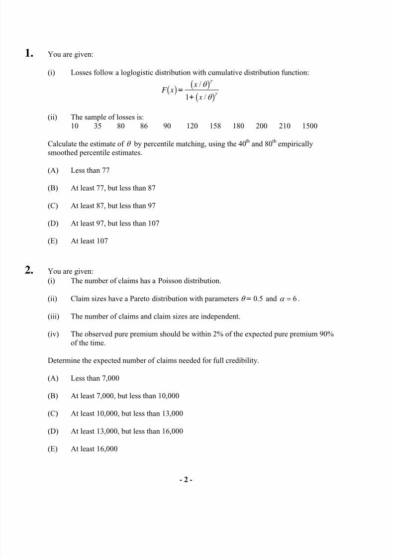
1. You are given:
(i) Losses follow a loglogistic distribution with cumulative distribution function:
F x x
x
b g b g
b g
/
/
θ
θ
γ
γ
1
(ii) The sample of losses is:10 35 80 86 90 120 158 180 200 210 1500
Calculate the estimate of θ by percentile matching, using the 40th and 80th empiricallysmoothed percentile estimates.
(A) Less than 77
(B) At least 77, but less than 87
(C) At least 87, but less than 97
(D) At least 97, but less than 107
(E) At least 107
2. You are given:(i) The number of claims has a Poisson distribution.
(ii) Claim sizes have a Pareto distribution with parameters θ = 0.5 and α = 6 .
(iii) The number of claims and claim sizes are independent.
(iv) The observed pure premium should be within 2% of the expected pure premium 90%of the time.
Determine the expected number of claims needed for full credibility.
(A) Less than 7,000
(B) At least 7,000, but less than 10,000
(C) At least 10,000, but less than 13,000
(D) At least 13,000, but less than 16,000
(E) At least 16,000
8/13/2019 Edu Exam c Sample Quest
http://slidepdf.com/reader/full/edu-exam-c-sample-quest 3/184
- 3 -
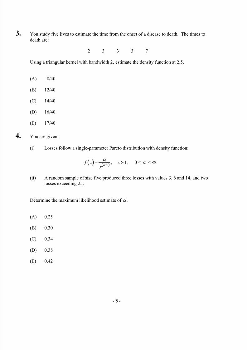
3. You study five lives to estimate the time from the onset of a disease to death. The times todeath are:
2 3 3 3 7
Using a triangular kernel with bandwidth 2, estimate the density function at 2.5.
(A) 8/40
(B) 12/40
(C) 14/40
(D) 16/40
(E) 17/40
4. You are given:
(i) Losses follow a single-parameter Pareto distribution with density function:
1 , 1 f x x
x α
α
> , 0 < α < ∞
(ii) A random sample of size five produced three losses with values 3, 6 and 14, and two
losses exceeding 25.
Determine the maximum likelihood estimate of α .
(A) 0.25
(B) 0.30
(C) 0.34
(D) 0.38
(E) 0.42
8/13/2019 Edu Exam c Sample Quest
http://slidepdf.com/reader/full/edu-exam-c-sample-quest 4/184
- 4 -
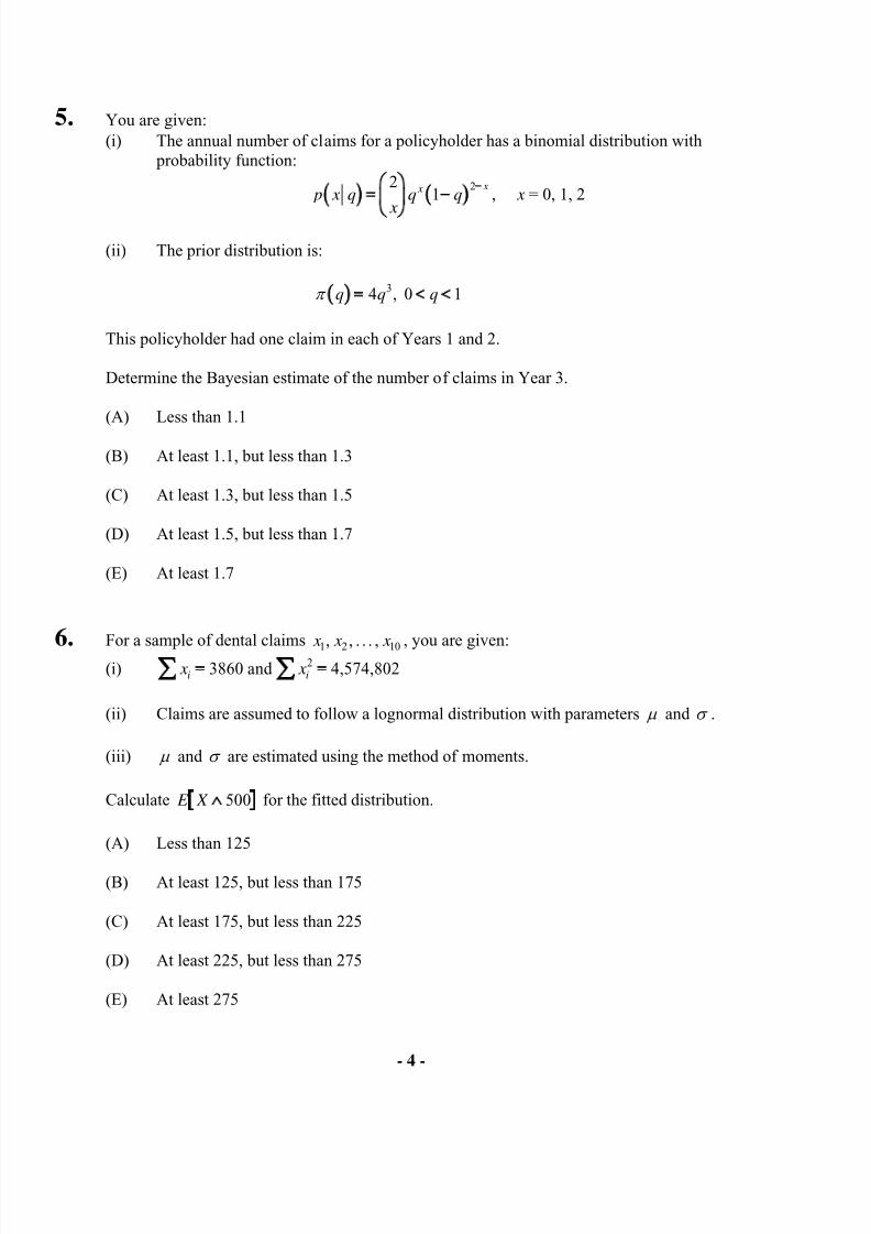
5. You are given:(i) The annual number of claims for a policyholder has a binomial distribution with
probability function:
221
x x p x q q q
x
, x = 0, 1, 2
(ii) The prior distribution is:
34 , 0 1q q qπ = < <
This policyholder had one claim in each of Years 1 and 2.
Determine the Bayesian estimate of the number of claims in Year 3.
(A) Less than 1.1
(B) At least 1.1, but less than 1.3
(C) At least 1.3, but less than 1.5
(D) At least 1.5, but less than 1.7
(E) At least 1.7
6. For a sample of dental claims 1 2 10, , . . . , x x x , you are given:(i) 23860 and 4,574,802i i x x =∑
(ii) Claims are assumed to follow a lognormal distribution with parameters µ and σ .
(iii) µ and σ are estimated using the method of moments.
Calculate E X ∧ 500 for the fitted distribution.
(A) Less than 125
(B) At least 125, but less than 175
(C) At least 175, but less than 225
(D) At least 225, but less than 275
(E) At least 275
8/13/2019 Edu Exam c Sample Quest
http://slidepdf.com/reader/full/edu-exam-c-sample-quest 5/184
- 5 -
7. DELETED
8. You are given:(i) Claim counts follow a Poisson distribution with mean θ .
(ii) Claim sizes follow an exponential distribution with mean 10θ .
(iii) Claim counts and claim sizes are independent, given θ .
(iv) The prior distribution has probability density function:
π θ θ
b g = 56
, θ > 1
Calculate Bühlmann’s k for aggregate losses.(A) Less than 1
(B) At least 1, but less than 2
(C) At least 2, but less than 3
(D) At least 3, but less than 4
(E) At least 4
9. DELETED
10. DELETED
8/13/2019 Edu Exam c Sample Quest
http://slidepdf.com/reader/full/edu-exam-c-sample-quest 6/184
- 6 -
11. You are given:
(i) Losses on a company’s insurance policies follow a Pareto distribution with probability density function:
2 , 0 f x x
x
θ θ
θ = < < ∞
(ii) For half of the company’s policies θ = 1 , while for the other half θ = 3 .
For a randomly selected policy, losses in Year 1 were 5.
Determine the posterior probability that losses for this policy in Year 2 will exceed 8.
(A) 0.11
(B) 0.15
(C) 0.19
(D) 0.21
(E) 0.27
12. You are given total claims for two policyholders:
YearPolicyholder 1 2 3 4
X 730 800 650 700Y 655 650 625 750
Using the nonparametric empirical Bayes method, determine the Bühlmann credibility premium for Policyholder Y.
(A) 655
(B) 670
(C) 687
(D) 703
(E) 719
8/13/2019 Edu Exam c Sample Quest
http://slidepdf.com/reader/full/edu-exam-c-sample-quest 7/184
- 7 -
13. A particular line of business has three types of claims. The historical probability and thenumber of claims for each type in the current year are:
TypeHistorical
Probability Number of Claims
in Current Year
A 0.2744 112
B 0.3512 180
C 0.3744 138
You test the null hypothesis that the probability of each type of claim in the current year isthe same as the historical probability.
Calculate the chi-square goodness-of-fit test statistic.
(A) Less than 9
(B) At least 9, but less than 10
(C) At least 10, but less than 11
(D) At least 11, but less than 12
(E) At least 12
14. The information associated with the maximum likelihood estimator of a parameter θ is 4n ,where n is the number of observations.
Calculate the asymptotic variance of the maximum likelihood estimator of 2θ .
(A) 12n
(B) 1n
(C) 4n
(D) 8n
(E) 16n
8/13/2019 Edu Exam c Sample Quest
http://slidepdf.com/reader/full/edu-exam-c-sample-quest 8/184
- 8 -
15. You are given:
(i) The probability that an insured will have at least one loss during any year is p.
(ii) The prior distribution for p is uniform on [ ]0,0.5 .
(iii) An insured is observed for 8 years and has at least one loss every year.
Determine the posterior probability that the insured will have at least one loss during Year 9.
(A) 0.450
(B) 0.475
(C) 0.500
(D) 0.550
(E) 0.625
16-17. Use the following information for questions 16 and 17. For a survival study with censored and truncated data, you are given:
Time (t ) Number at Risk
at Time t Failures at Time t 1 30 52 27 93 32 64 25 55 20 4
16. The probability of failing at or before Time 4, given survival past Time 1, is 3 1q .
Calculate Greenwood’s approximation of the variance of 3 1q .
(A) 0.0067
(B) 0.0073
(C) 0.0080
(D) 0.0091
(E) 0.0105
8/13/2019 Edu Exam c Sample Quest
http://slidepdf.com/reader/full/edu-exam-c-sample-quest 9/184
- 9 -
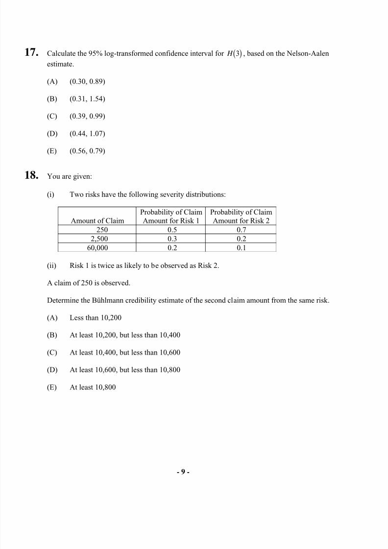
17. Calculate the 95% log-transformed confidence interval for H 3b g , based on the Nelson-Aalen
estimate.
(A) (0.30, 0.89)
(B) (0.31, 1.54)
(C) (0.39, 0.99)
(D) (0.44, 1.07)
(E) (0.56, 0.79)
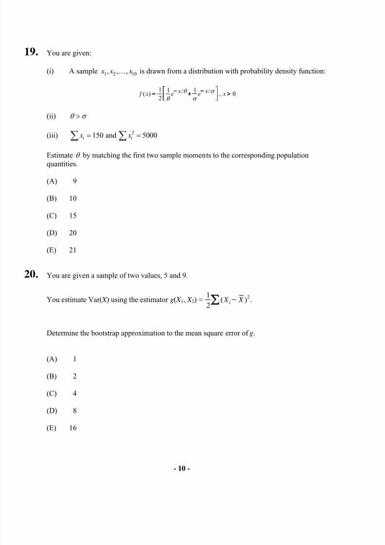
18. You are given:
(i) Two risks have the following severity distributions:
Amount of ClaimProbability of ClaimAmount for Risk 1
Probability of ClaimAmount for Risk 2
250 0.5 0.72,500 0.3 0.2
60,000 0.2 0.1
(ii) Risk 1 is twice as likely to be observed as Risk 2.
A claim of 250 is observed.
Determine the Bühlmann credibility estimate of the second claim amount from the same risk.
(A) Less than 10,200
(B) At least 10,200, but less than 10,400
(C) At least 10,400, but less than 10,600
(D) At least 10,600, but less than 10,800
(E) At least 10,800
8/13/2019 Edu Exam c Sample Quest
http://slidepdf.com/reader/full/edu-exam-c-sample-quest 10/184
- 10 -
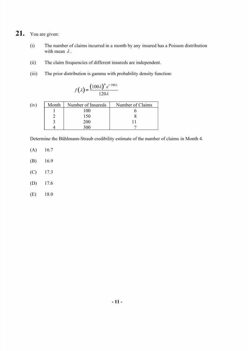
19. You are given:
(i) A sample x x x1 2 10, , , is drawn from a distribution with probability density function:
1 1 1/ /( ) , 02
x x f x e e x
θ σ
θ σ
= >
(ii) θ σ >
(iii) x xi i= =∑∑ 150 50002 and
Estimate θ by matching the first two sample moments to the corresponding populationquantities.
(A) 9
(B) 10
(C) 15
(D) 20
(E) 21
20. You are given a sample of two values, 5 and 9.
You estimate Var( X ) using the estimator g( X 1, X 2) =21
( ) .2
i X X
Determine the bootstrap approximation to the mean square error of g.
(A) 1
(B) 2
(C) 4
(D) 8
(E) 16
8/13/2019 Edu Exam c Sample Quest
http://slidepdf.com/reader/full/edu-exam-c-sample-quest 11/184
- 11 -
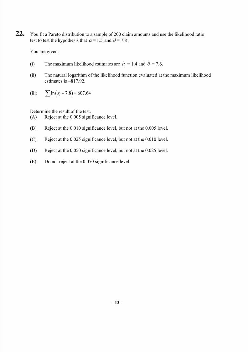
21. You are given:
(i) The number of claims incurred in a month by any insured has a Poisson distributionwith mean λ .
(ii) The claim frequencies of different insureds are independent.
(iii) The prior distribution is gamma with probability density function:
6 100100
120
e f
λ λ λ
λ
=
(iv) Month Number of Insureds Number of Claims1 100 62 150 8
3 200 114 300 ?
Determine the Bühlmann-Straub credibility estimate of the number of claims in Month 4.
(A) 16.7
(B) 16.9
(C) 17.3
(D) 17.6
(E) 18.0
8/13/2019 Edu Exam c Sample Quest
http://slidepdf.com/reader/full/edu-exam-c-sample-quest 12/184
- 12 -
22. You fit a Pareto distribution to a sample of 200 claim amounts and use the likelihood ratiotest to test the hypothesis that 1.5α = and 7.8θ = .
You are given:
(i) The maximum likelihood estimates are α = 1.4 and θ = 7.6.
(ii) The natural logarithm of the likelihood function evaluated at the maximum likelihoodestimates is −817.92.
(iii) ( )ln 7.8 607.64i x + =∑
Determine the result of the test.(A) Reject at the 0.005 significance level.
(B) Reject at the 0.010 significance level, but not at the 0.005 level.
(C) Reject at the 0.025 significance level, but not at the 0.010 level.
(D) Reject at the 0.050 significance level, but not at the 0.025 level.
(E) Do not reject at the 0.050 significance level.
8/13/2019 Edu Exam c Sample Quest
http://slidepdf.com/reader/full/edu-exam-c-sample-quest 13/184
- 13 -
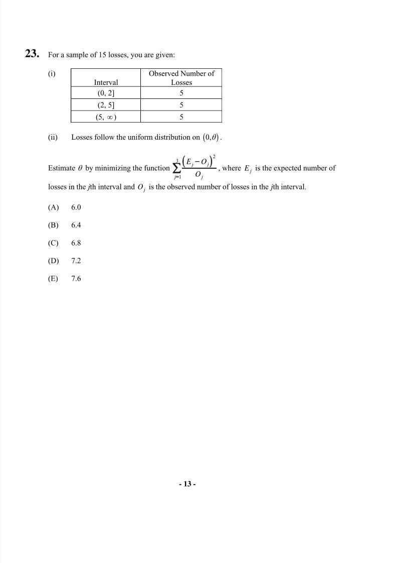
23. For a sample of 15 losses, you are given:
(i) Interval
Observed Number ofLosses
(0, 2] 5
(2, 5] 5
(5, ∞ ) 5
(ii) Losses follow the uniform distribution on 0,θ b g .
Estimate θ by minimizing the function
23
1
j j
j j
E O
O ∑ , where j E is the expected number of
losses in the jth interval and jO is the observed number of losses in the jth interval.
(A) 6.0
(B) 6.4
(C) 6.8
(D) 7.2
(E) 7.6
8/13/2019 Edu Exam c Sample Quest
http://slidepdf.com/reader/full/edu-exam-c-sample-quest 14/184
- 14 -
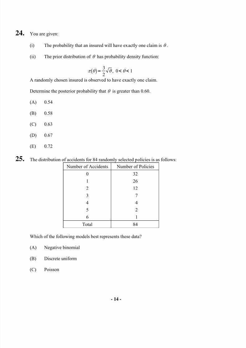
24. You are given:
(i) The probability that an insured will have exactly one claim is θ .
(ii) The prior distribution of θ has probability density function:
π θ θ θ b g = < <3
20 1,
A randomly chosen insured is observed to have exactly one claim.
Determine the posterior probability that θ is greater than 0.60.
(A) 0.54
(B) 0.58
(C) 0.63
(D) 0.67
(E) 0.72
25. The distribution of accidents for 84 randomly selected policies is as follows:
Number of Accidents Number of Policies
0 32
1 262 12
3 7
4 4
5 2
6 1
Total 84
Which of the following models best represents these data?
(A) Negative binomial
(B) Discrete uniform
(C) Poisson
8/13/2019 Edu Exam c Sample Quest
http://slidepdf.com/reader/full/edu-exam-c-sample-quest 15/184
- 15 -
(D) Binomial
(E) Either Poisson or Binomial
26. You are given:
(i) Low-hazard risks have an exponential claim size distribution with mean θ .
(ii) Medium-hazard risks have an exponential claim size distribution with mean 2θ .
(iii) High-hazard risks have an exponential claim size distribution with mean 3θ .
(iv) No claims from low-hazard risks are observed.
(v) Three claims from medium-hazard risks are observed, of sizes 1, 2 and 3.
(vi) One claim from a high-hazard risk is observed, of size 15.
Determine the maximum likelihood estimate of θ .
(A) 1
(B) 2
(C) 3
(D) 4
(E) 5
8/13/2019 Edu Exam c Sample Quest
http://slidepdf.com/reader/full/edu-exam-c-sample-quest 16/184
- 16 -
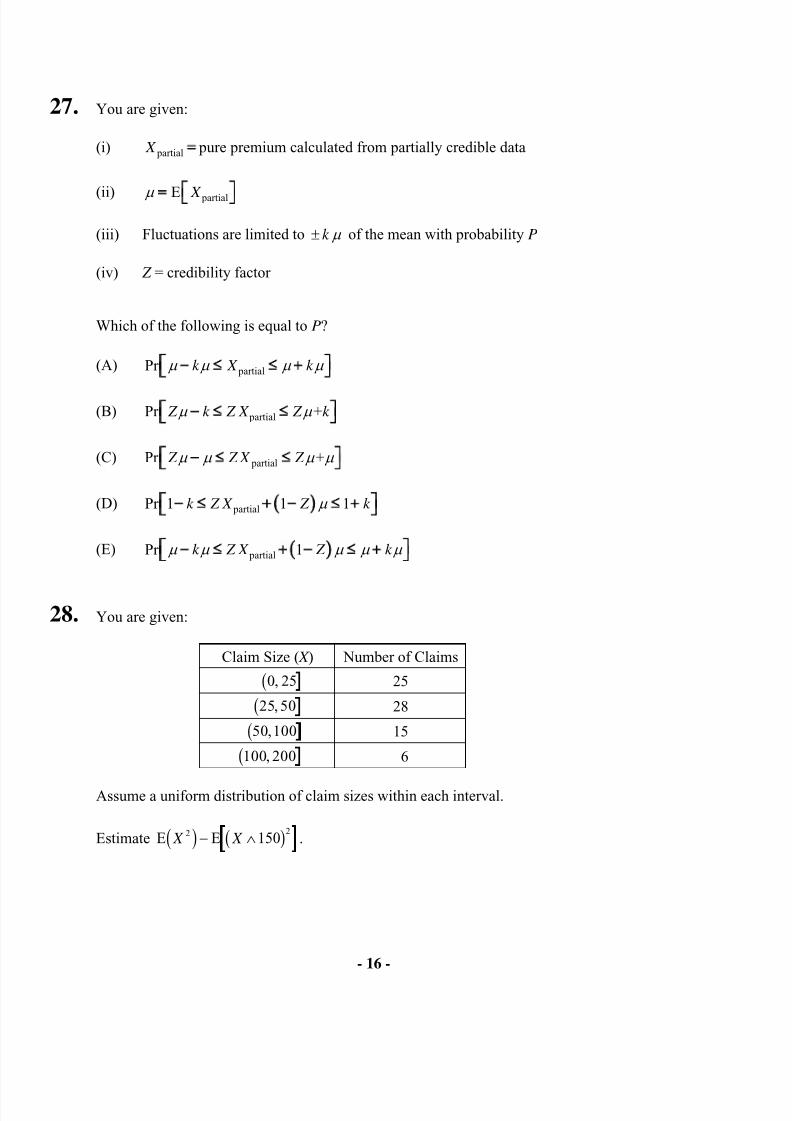
27. You are given:
(i) partial X = pure premium calculated from partially credible data
(ii) partialE X µ
(iii) Fluctuations are limited to ± k µ of the mean with probability P
(iv) Z = credibility factor
Which of the following is equal to P?
(A) partialPr k X k µ µ µ µ ≤ ≤
(B) partialPr + Z k Z X Z k µ µ ≤ ≤
(C) partialPr + Z Z X Z µ µ µ µ ≤ ≤
(D) partialPr 1 1 1k Z X Z k µ ≤ ≤
(E) partialPr 1k Z X Z k µ µ µ µ µ ≤ ≤
28. You are given:
Claim Size ( X ) Number of Claims
0 25,b 25
25 50,b 28
50 100,b 15
100 200,b 6
Assume a uniform distribution of claim sizes within each interval.
Estimate E E X X 2 2150c h b g− ∧ .
8/13/2019 Edu Exam c Sample Quest
http://slidepdf.com/reader/full/edu-exam-c-sample-quest 17/184
- 17 -
(A) Less than 200
(B) At least 200, but less than 300
(C) At least 300, but less than 400
(D) At least 400, but less than 500
(E) At least 500
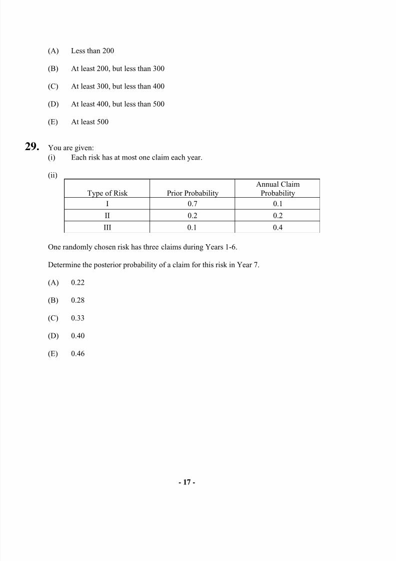
29. You are given:(i) Each risk has at most one claim each year.
(ii)
Type of Risk Prior Probability
Annual Claim
ProbabilityI 0.7 0.1
II 0.2 0.2
III 0.1 0.4
One randomly chosen risk has three claims during Years 1-6.
Determine the posterior probability of a claim for this risk in Year 7.
(A) 0.22
(B) 0.28
(C) 0.33
(D) 0.40
(E) 0.46
8/13/2019 Edu Exam c Sample Quest
http://slidepdf.com/reader/full/edu-exam-c-sample-quest 18/184
- 18 -
30. You are given the following about 100 insurance policies in a study of time to policysurrender:(i) The study was designed in such a way that for every policy that was surrendered, a
new policy was added, meaning that the risk set, jr , is always equal to 100.
(ii) Policies are surrendered only at the end of a policy year.
(iii) The number of policies surrendered at the end of each policy year was observed to be:
1 at the end of the 1st policy year2 at the end of the 2nd policy year3 at the end of the 3rd policy year n at the end of the n
th policy year
(iv) The Nelson-Aalen empirical estimate of the cumulative distribution function at timen, )(ˆ nF , is 0.542.
What is the value of n?(A) 8
(B) 9
(C) 10
(D) 11
(E) 12
31. You are given the following claim data for automobile policies:200 255 295 320 360 420 440 490 500 520 1020
Calculate the smoothed empirical estimate of the 45th percentile.
(A) 358
(B) 371
(C) 384
(D) 390
(E) 396
8/13/2019 Edu Exam c Sample Quest
http://slidepdf.com/reader/full/edu-exam-c-sample-quest 19/184
- 19 -
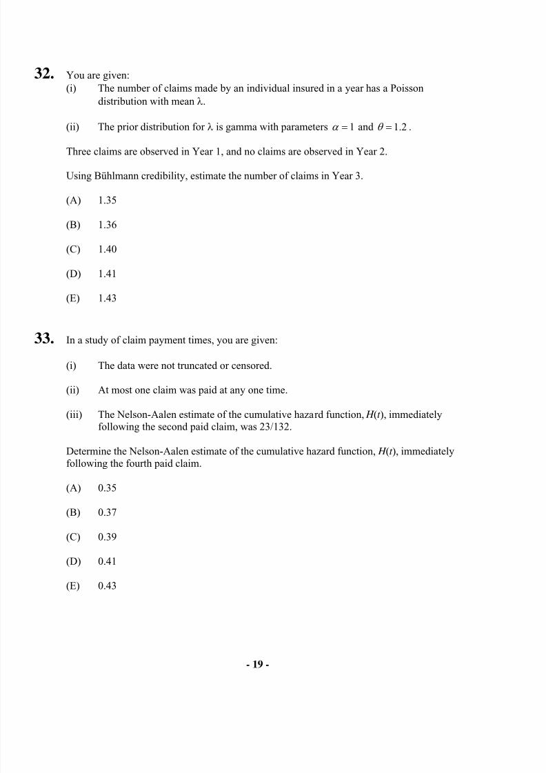
32. You are given:(i) The number of claims made by an individual insured in a year has a Poisson
distribution with mean λ.
(ii) The prior distribution for λ is gamma with parameters α = 1 and θ = 1.2 .
Three claims are observed in Year 1, and no claims are observed in Year 2.
Using Bühlmann credibility, estimate the number of claims in Year 3.
(A) 1.35
(B) 1.36
(C) 1.40
(D) 1.41
(E) 1.43
33. In a study of claim payment times, you are given:
(i) The data were not truncated or censored.
(ii) At most one claim was paid at any one time.
(iii) The Nelson-Aalen estimate of the cumulative hazard function, H (t ), immediatelyfollowing the second paid claim, was 23/132.
Determine the Nelson-Aalen estimate of the cumulative hazard function, H (t ), immediatelyfollowing the fourth paid claim.
(A) 0.35
(B) 0.37
(C) 0.39(D) 0.41
(E) 0.43

8/13/2019 Edu Exam c Sample Quest
http://slidepdf.com/reader/full/edu-exam-c-sample-quest 20/184
- 20 -
34. The number of claims follows a negative binomial distribution with parameters β and r ,
where β is unknown and r is known. You wish to estimate β based on n observations,
where x is the mean of these observations.
Determine the maximum likelihood estimate of β .
(A)2
x
r
(B) x
r
(C) x
(D) rx
(E) 2r x
35. You are given the following information about a credibility model:
First Observation Unconditional ProbabilityBayesian Estimate ofSecond Observation
1 1/3 1.50
2 1/3 1.503 1/3 3.00
Determine the Bühlmann credibility estimate of the second observation, given that the firstobservation is 1.
(A) 0.75
(B) 1.00
(C) 1.25
(D) 1.50
(E) 1.75
8/13/2019 Edu Exam c Sample Quest
http://slidepdf.com/reader/full/edu-exam-c-sample-quest 21/184
- 21 -
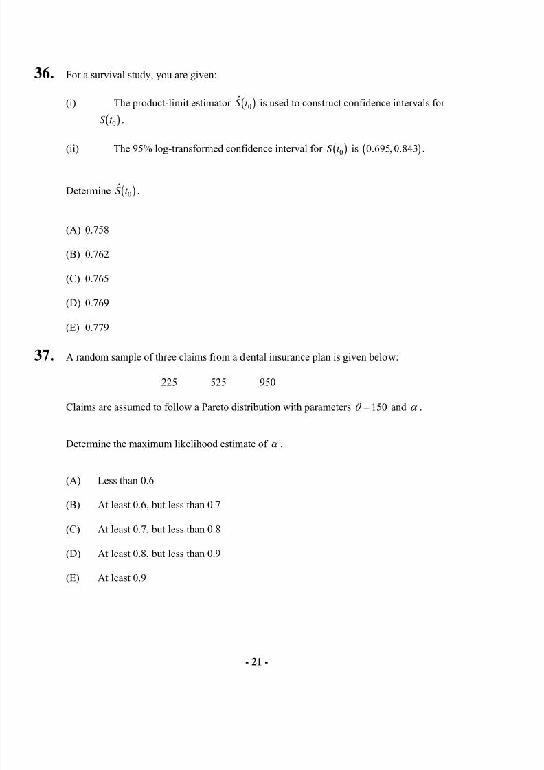
36. For a survival study, you are given:
(i) The product-limit estimator S t 0b g is used to construct confidence intervals for
S t 0b g .
(ii) The 95% log-transformed confidence interval for S t 0b g is 0.695 0.843,b g .
Determine S t 0b g .
(A) 0.758
(B) 0.762
(C) 0.765
(D) 0.769
(E) 0.779
37. A random sample of three claims from a dental insurance plan is given below:
225 525 950
Claims are assumed to follow a Pareto distribution with parameters θ = 150 and α .
Determine the maximum likelihood estimate of α .
(A) Less than 0.6
(B) At least 0.6, but less than 0.7
(C) At least 0.7, but less than 0.8
(D) At least 0.8, but less than 0.9
(E) At least 0.9
8/13/2019 Edu Exam c Sample Quest
http://slidepdf.com/reader/full/edu-exam-c-sample-quest 22/184
- 22 -
38. An insurer has data on losses for four policyholders for 7 years. The loss from the ith policyholder for year j is X ij .
You are given:
X X ij i
ji
− ===
∑∑ d i1
7
1
4 2 33.60
X X i
i
− ==
∑ c h2
1
4
3.30
Using nonparametric empirical Bayes estimation, calculate the Bühlmann credibility factorfor an individual policyholder.
(A) Less than 0.74
(B) At least 0.74, but less than 0.77
(C) At least 0.77, but less than 0.80
(D) At least 0.80, but less than 0.83
(E) At least 0.83
39. You are given the following information about a commercial auto liability book of business:
(i) Each insured’s claim count has a Poisson distribution with mean λ , where λ has agamma distribution with α = 15. and θ = 0 2. .
(ii) Individual claim size amounts are independent and exponentially distributed withmean 5000.
(iii) The full credibility standard is for aggregate losses to be within 5% of the expectedwith probability 0.90.
Using classical credibility, determine the expected number of claims required for fullcredibility.
8/13/2019 Edu Exam c Sample Quest
http://slidepdf.com/reader/full/edu-exam-c-sample-quest 23/184
- 23 -
(A) 2165
(B) 2381
(C) 3514
(D) 7216
(E) 7938
40. You are given:
(i) A sample of claim payments is:
29 64 90 135 182
(ii) Claim sizes are assumed to follow an exponential distribution.
(iii) The mean of the exponential distribution is estimated using the method of moments.
Calculate the value of the Kolmogorov-Smirnov test statistic.
(A) 0.14
(B) 0.16
(C) 0.19
(D) 0.25
(E) 0.27
41. You are given:
(i) Annual claim frequency for an individual policyholder has mean λ and variance 2σ .
(ii) The prior distribution for λ is uniform on the interval [0.5, 1.5].
(iii) The prior distribution for 2σ is exponential with mean 1.25.
A policyholder is selected at random and observed to have no claims in Year 1.
Using Bühlmann credibility, estimate the number of claims in Year 2 for the selected policyholder.
8/13/2019 Edu Exam c Sample Quest
http://slidepdf.com/reader/full/edu-exam-c-sample-quest 24/184
- 24 -
(A) 0.56
(B) 0.65
(C) 0.71
(D) 0.83
(E) 0.94
42. DELETED
43. You are given:
(i) The prior distribution of the parameter Θ has probability density function:
π θ θ
θ b g = < < ∞1
12 ,
(ii) Given Θ = θ , claim sizes follow a Pareto distribution with parameters α = 2 and θ .
A claim of 3 is observed.
Calculate the posterior probability that Θ exceeds 2.
(A) 0.33
(B) 0.42
(C) 0.50
(D) 0.58
(E) 0.64
8/13/2019 Edu Exam c Sample Quest
http://slidepdf.com/reader/full/edu-exam-c-sample-quest 25/184
- 25 -
44. You are given:
(i) Losses follow an exponential distribution with mean θ .
(ii) A random sample of 20 losses is distributed as follows:
Loss Range Frequency
[0, 1000] 7
(1000, 2000] 6
(2000, ∞ ) 7
Calculate the maximum likelihood estimate of θ .
(A) Less than 1950
(B) At least 1950, but less than 2100
(C) At least 2100, but less than 2250
(D) At least 2250, but less than 2400
(E) At least 2400
45. You are given:
(i) The amount of a claim, X , is uniformly distributed on the interval 0,θ .
(ii) The prior density of θ π θ θ
θ is b g = >500
5002 , .
Two claims, x1 400= and x2 600= , are observed. You calculate the posteriordistribution as:
f x xθ θ
θ 1 2
3
43
600600, ,c h =
F H G
I K J
>
Calculate the Bayesian premium, E X x x3 1 2,c h .
8/13/2019 Edu Exam c Sample Quest
http://slidepdf.com/reader/full/edu-exam-c-sample-quest 26/184
- 26 -
(A) 450
(B) 500
(C) 550
(D) 600
(E) 650
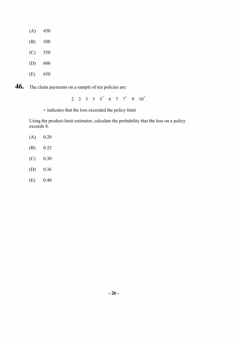
46. The claim payments on a sample of ten policies are:
2 3 3 5 5+ 6 7 7
+ 9 10
+
+ indicates that the loss exceeded the policy limit
Using the product-limit estimator, calculate the probability that the loss on a policyexceeds 8.
(A) 0.20
(B) 0.25
(C) 0.30
(D) 0.36
(E) 0.40
8/13/2019 Edu Exam c Sample Quest
http://slidepdf.com/reader/full/edu-exam-c-sample-quest 27/184
- 27 -
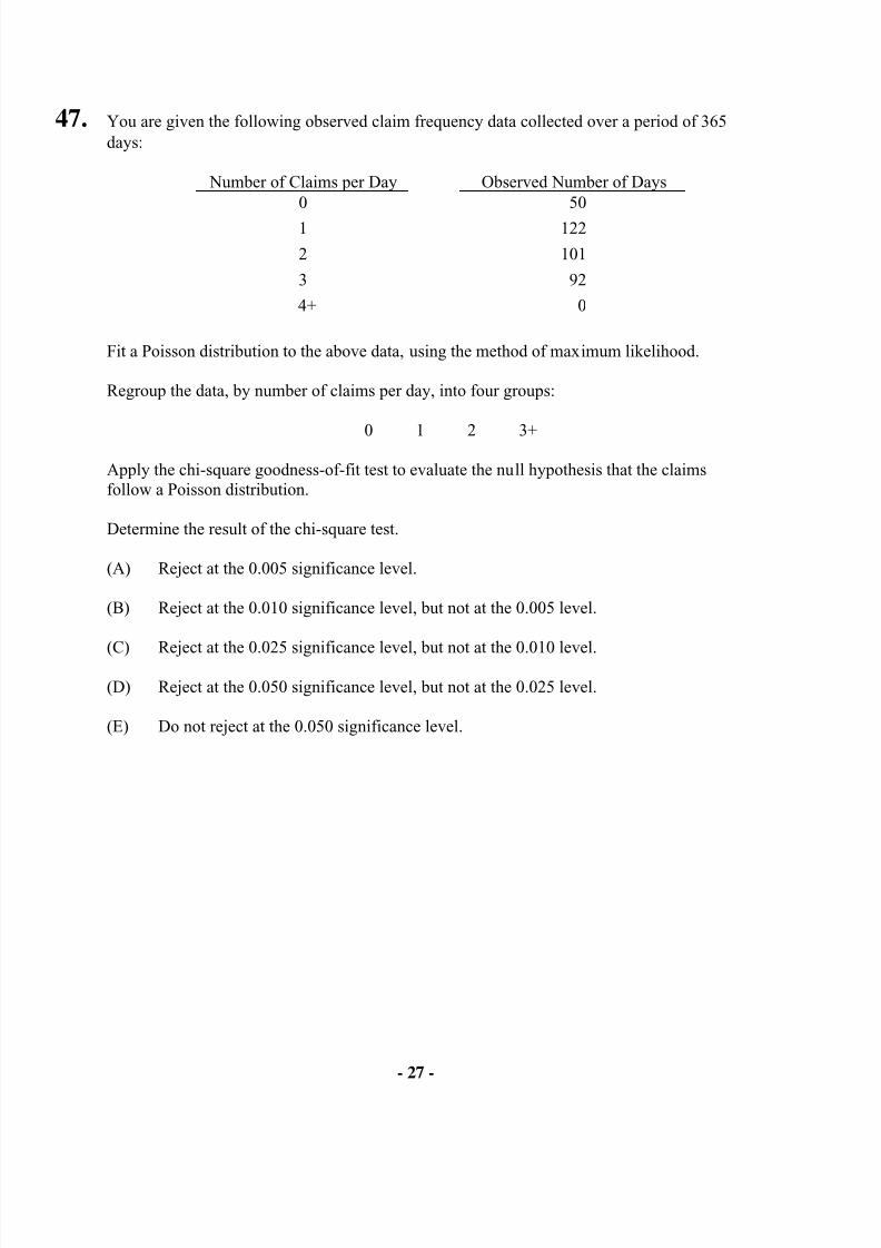
47. You are given the following observed claim frequency data collected over a period of 365days:
Number of Claims per Day Observed Number of Days0 50
1 122
2 101
3 92
4+ 0
Fit a Poisson distribution to the above data, using the method of maximum likelihood.
Regroup the data, by number of claims per day, into four groups:
0 1 2 3+
Apply the chi-square goodness-of-fit test to evaluate the null hypothesis that the claimsfollow a Poisson distribution.
Determine the result of the chi-square test.
(A) Reject at the 0.005 significance level.
(B) Reject at the 0.010 significance level, but not at the 0.005 level.
(C) Reject at the 0.025 significance level, but not at the 0.010 level.(D) Reject at the 0.050 significance level, but not at the 0.025 level.
(E) Do not reject at the 0.050 significance level.
8/13/2019 Edu Exam c Sample Quest
http://slidepdf.com/reader/full/edu-exam-c-sample-quest 28/184
- 28 -
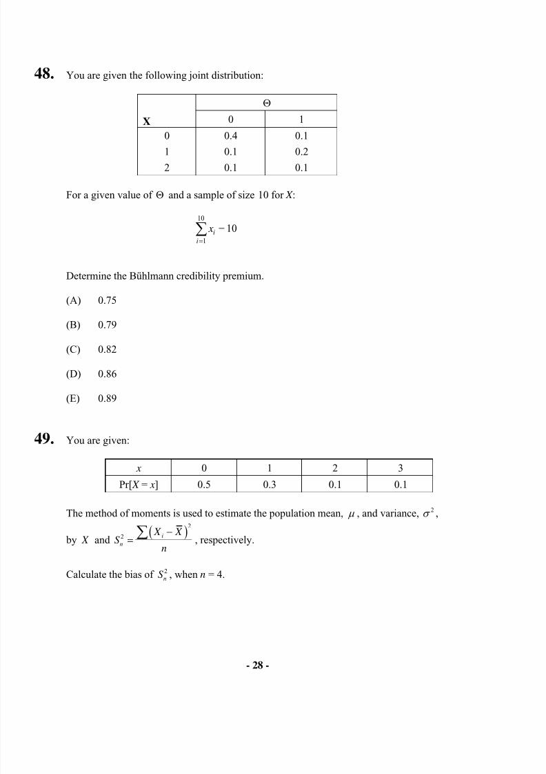
48. You are given the following joint distribution:
X
Θ
0 1
0 0.4 0.11 0.1 0.2
2 0.1 0.1
For a given value of Θ and a sample of size 10 for X :
xi
i =∑ =
1
10
10
Determine the Bühlmann credibility premium.
(A) 0.75
(B) 0.79
(C) 0.82
(D) 0.86
(E) 0.89
49. You are given:
x 0 1 2 3
Pr[ X = x] 0.5 0.3 0.1 0.1
The method of moments is used to estimate the population mean, µ , and variance, 2σ ,
by X and
( )2
2 i
n
X X
S n
−
=
∑, respectively.
Calculate the bias of 2nS , when n = 4.
8/13/2019 Edu Exam c Sample Quest
http://slidepdf.com/reader/full/edu-exam-c-sample-quest 29/184
- 29 -
(A) –0.72
(B) –0.49
(C) –0.24
(D) –0.08
(E) 0.00
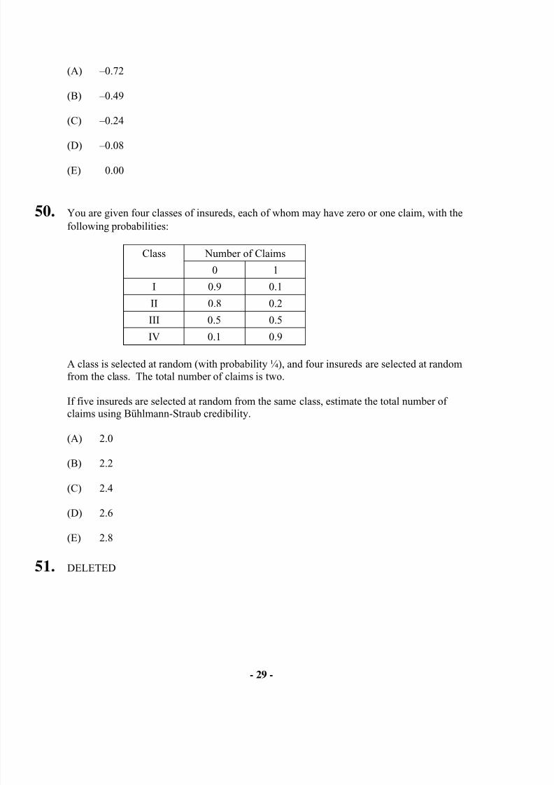
50. You are given four classes of insureds, each of whom may have zero or one claim, with thefollowing probabilities:
Class Number of Claims
0 1I 0.9 0.1
II 0.8 0.2
III 0.5 0.5
IV 0.1 0.9
A class is selected at random (with probability ¼), and four insureds are selected at randomfrom the class. The total number of claims is two.
If five insureds are selected at random from the same class, estimate the total number of
claims using Bühlmann-Straub credibility.
(A) 2.0
(B) 2.2
(C) 2.4
(D) 2.6
(E) 2.8
51. DELETED
8/13/2019 Edu Exam c Sample Quest
http://slidepdf.com/reader/full/edu-exam-c-sample-quest 30/184
- 30 -
52. With the bootstrapping technique, the underlying distribution function is estimated by whichof the following?
(A) The empirical distribution function
(B) A normal distribution function
(C) A parametric distribution function selected by the modeler
(D) Any of (A), (B) or (C)
(E) None of (A), (B) or (C)
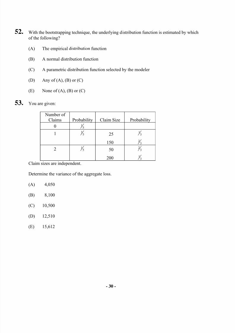
53. You are given:
Number ofClaims Probability Claim Size Probability
0 15
1 35 25
150
13
23
2 15 50
200
23
13
Claim sizes are independent.
Determine the variance of the aggregate loss.
(A) 4,050
(B) 8,100
(C) 10,500
(D) 12,510
(E) 15,612
8/13/2019 Edu Exam c Sample Quest
http://slidepdf.com/reader/full/edu-exam-c-sample-quest 31/184
- 31 -
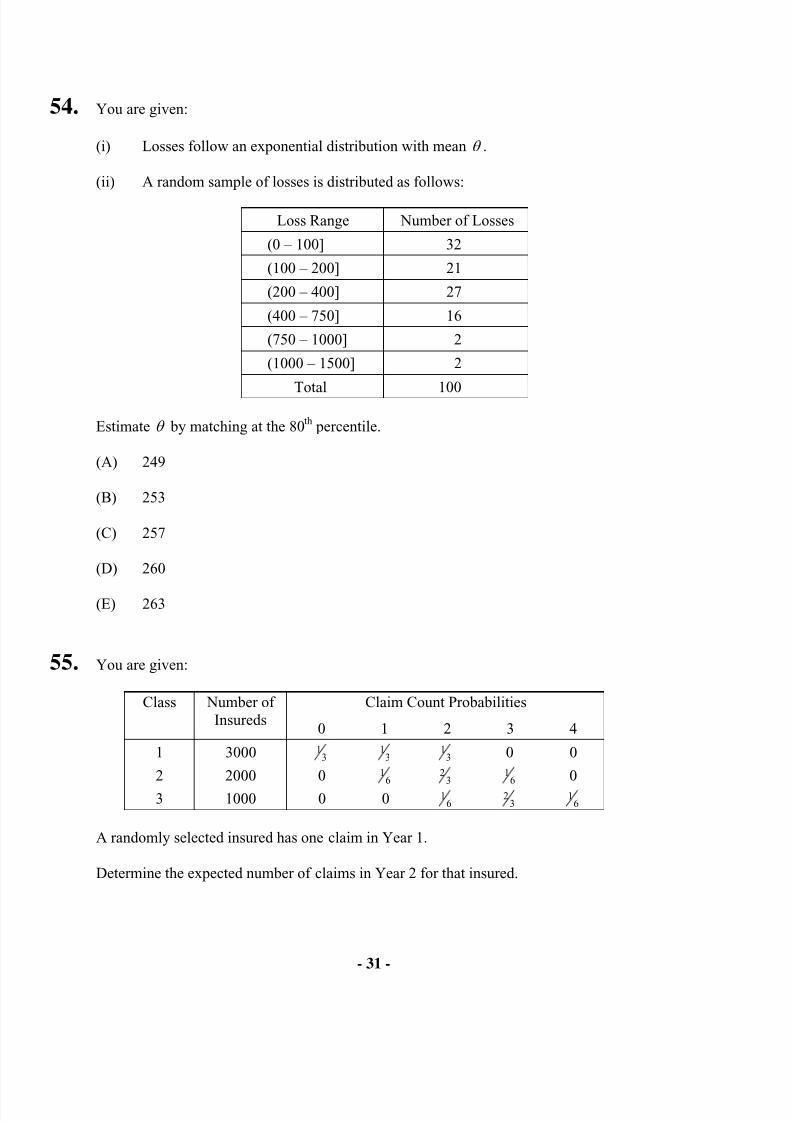
54. You are given:
(i) Losses follow an exponential distribution with mean θ .
(ii) A random sample of losses is distributed as follows:
Loss Range Number of Losses
(0 – 100] 32
(100 – 200] 21
(200 – 400] 27
(400 – 750] 16
(750 – 1000] 2
(1000 – 1500] 2
Total 100
Estimate θ by matching at the 80th percentile.
(A) 249
(B) 253
(C) 257
(D) 260
(E) 263
55. You are given:
Class Number ofInsureds
Claim Count Probabilities
0 1 2 3 4
1 3000 13 1
3 13 0 0
2 2000 0 1
6
2
3
1
6
0
3 1000 0 0 16 2
3 16
A randomly selected insured has one claim in Year 1.
Determine the expected number of claims in Year 2 for that insured.
8/13/2019 Edu Exam c Sample Quest
http://slidepdf.com/reader/full/edu-exam-c-sample-quest 32/184
- 32 -
(A) 1.00
(B) 1.25
(C) 1.33
(D) 1.67
(E) 1.75
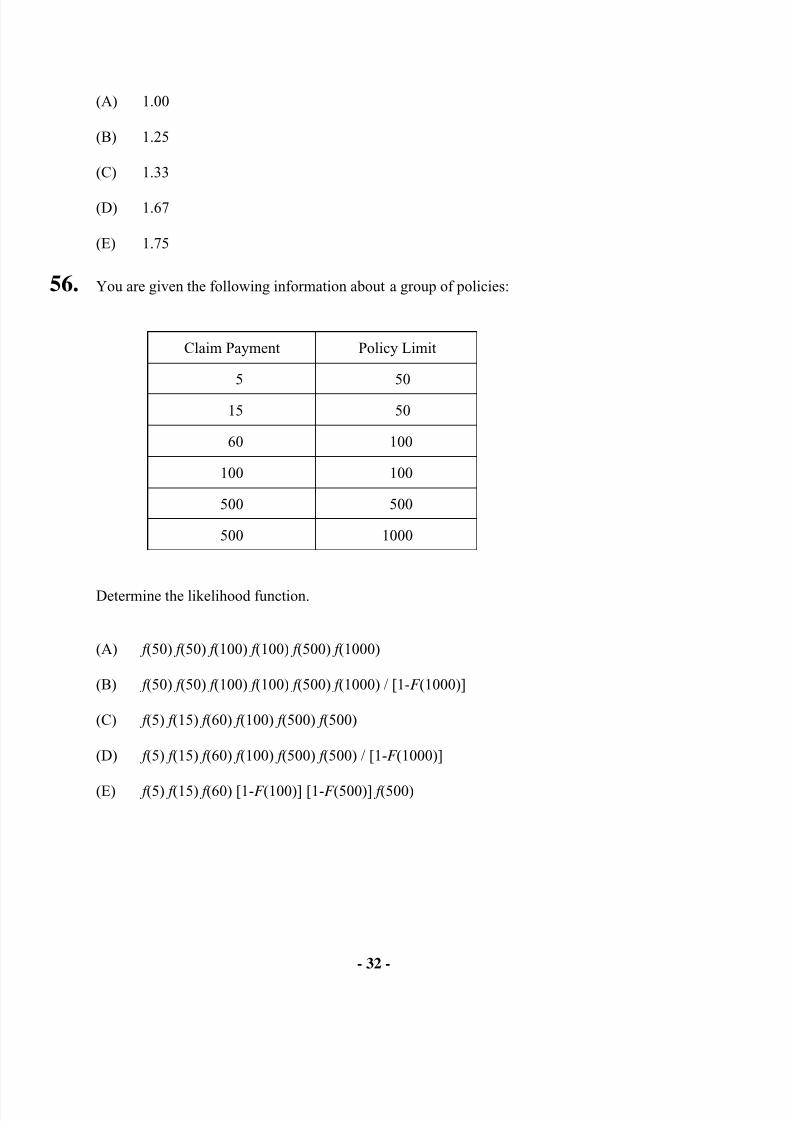
56. You are given the following information about a group of policies:
Claim Payment Policy Limit
5 50
15 50
60 100
100 100
500 500
500 1000
Determine the likelihood function.
(A) f (50) f (50) f (100) f (100) f (500) f (1000)
(B) f (50) f (50) f (100) f (100) f (500) f (1000) / [1-F (1000)]
(C) f (5) f (15) f (60) f (100) f (500) f (500)
(D) f (5) f (15) f (60) f (100) f (500) f (500) / [1-F (1000)]
(E) f (5) f (15) f (60) [1-F (100)] [1-F (500)] f (500)
8/13/2019 Edu Exam c Sample Quest
http://slidepdf.com/reader/full/edu-exam-c-sample-quest 33/184
- 33 -
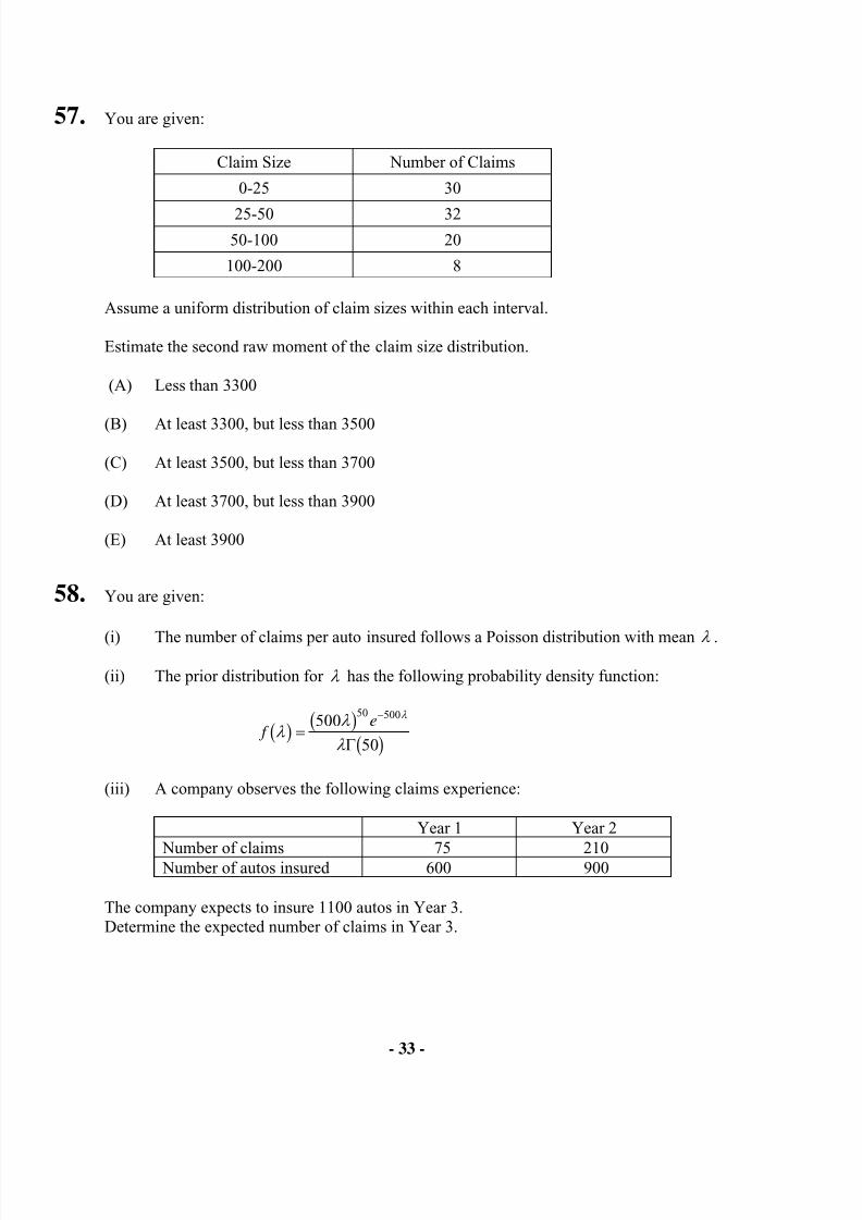
57. You are given:
Claim Size Number of Claims
0-25 30
25-50 3250-100 20
100-200 8
Assume a uniform distribution of claim sizes within each interval.
Estimate the second raw moment of the claim size distribution.
(A) Less than 3300
(B) At least 3300, but less than 3500
(C) At least 3500, but less than 3700
(D) At least 3700, but less than 3900
(E) At least 3900
58. You are given:
(i) The number of claims per auto insured follows a Poisson distribution with mean λ .
(ii) The prior distribution for λ has the following probability density function:
f e
λ λ
λ
λ
b g b gb g
=−500
50
50 500
Γ
(iii) A company observes the following claims experience:
Year 1 Year 2
Number of claims 75 210 Number of autos insured 600 900
The company expects to insure 1100 autos in Year 3.Determine the expected number of claims in Year 3.
8/13/2019 Edu Exam c Sample Quest
http://slidepdf.com/reader/full/edu-exam-c-sample-quest 34/184
- 34 -
(A) 178
(B) 184
(C) 193
(D) 209
(E) 224
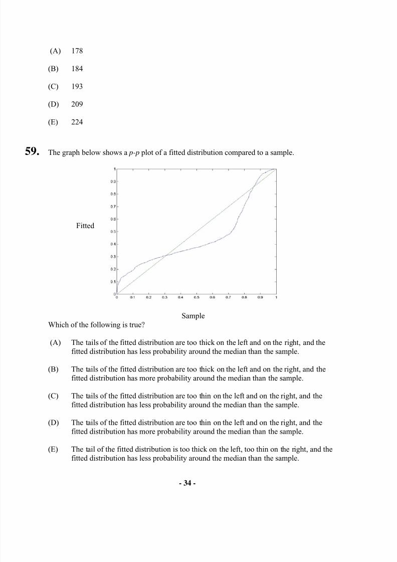
59. The graph below shows a p-p plot of a fitted distribution compared to a sample.
SampleWhich of the following is true?
(A) The tails of the fitted distribution are too thick on the left and on the right, and thefitted distribution has less probability around the median than the sample.
(B) The tails of the fitted distribution are too thick on the left and on the right, and thefitted distribution has more probability around the median than the sample.
(C) The tails of the fitted distribution are too thin on the left and on the right, and thefitted distribution has less probability around the median than the sample.
(D) The tails of the fitted distribution are too thin on the left and on the right, and thefitted distribution has more probability around the median than the sample.
(E) The tail of the fitted distribution is too thick on the left, too thin on the right, and thefitted distribution has less probability around the median than the sample.
Fitted
8/13/2019 Edu Exam c Sample Quest
http://slidepdf.com/reader/full/edu-exam-c-sample-quest 35/184
- 35 -
60. You are given the following information about six coins:
Coin Probability of Heads1 – 4 0.50
5 0.25
6 0.75
A coin is selected at random and then flipped repeatedly. i X denotes the outcome of the ith
flip, where “1” indicates heads and “0” indicates tails. The following sequence is obtained:
S X X X X = =1 2 3 4 1 1 0 1, , , , , ,l q l q
Determine E X S 5c h using Bayesian analysis.
(A) 0.52
(B) 0.54
(C) 0.56
(D) 0.59
(E) 0.63
61. You observe the following five ground-up claims from a data set that is truncated from belowat 100:
125 150 165 175 250You fit a ground-up exponential distribution using maximum likelihood estimation.
Determine the mean of the fitted distribution.
(A) 73
(B) 100
(C) 125
(D) 156
(E) 173
8/13/2019 Edu Exam c Sample Quest
http://slidepdf.com/reader/full/edu-exam-c-sample-quest 36/184
- 36 -
62. An insurer writes a large book of home warranty policies. You are given the followinginformation regarding claims filed by insureds against these policies:
(i) A maximum of one claim may be filed per year.
(ii) The probability of a claim varies by insured, and the claims experience for eachinsured is independent of every other insured.
(iii) The probability of a claim for each insured remains constant over time.
(iv) The overall probability of a claim being filed by a randomly selected insured in a yearis 0.10.
(v) The variance of the individual insured claim probabilities is 0.01.
An insured selected at random is found to have filed 0 claims over the past 10 years.
Determine the Bühlmann credibility estimate for the expected number of claims the selectedinsured will file over the next 5 years.
(A) 0.04
(B) 0.08
(C) 0.17
(D) 0.22
(E) 0.25
63. DELETED
64. For a group of insureds, you are given:
(i) The amount of a claim is uniformly distributed but will not exceed a certain unknownlimit θ .
(ii) The prior distribution of θ is π θ θ
θ b g = >500
5002 , .
(iii) Two independent claims of 400 and 600 are observed.
Determine the probability that the next claim will exceed 550.
8/13/2019 Edu Exam c Sample Quest
http://slidepdf.com/reader/full/edu-exam-c-sample-quest 37/184
- 37 -
(A) 0.19
(B) 0.22
(C) 0.25
(D) 0.28
(E) 0.31
65. You are given the following information about a general liability book of business comprisedof 2500 insureds:
(i) X Y i ij
j
N i
==
∑1
is a random variable representing the annual loss of the ith insured.
(ii) N N N 1 2 2500, , ..., are independent and identically distributed random variables
following a negative binomial distribution with parameters r = 2 and β = 0 2. .
(iii) Y Y Y i i iN i1 2, , ..., are independent and identically distributed random variables following
a Pareto distribution with α = 30. and θ = 1000 .
(iv) The full credibility standard is to be within 5% of the expected aggregate losses 90%of the time.
Using classical credibility theory, determine the partial credibility of the annual lossexperience for this book of business.
(A) 0.34
(B) 0.42
(C) 0.47
(D) 0.50
(E) 0.53
8/13/2019 Edu Exam c Sample Quest
http://slidepdf.com/reader/full/edu-exam-c-sample-quest 38/184
- 38 -
66. To estimate E X , you have simulated X X X X X 1 2 3 4 5, , , and with the following results:
1 2 3 4 5You want the standard deviation of the estimator of E X to be less than 0.05.
Estimate the total number of simulations needed.
(A) Less than 150
(B) At least 150, but less than 400
(C) At least 400, but less than 650
(D) At least 650, but less than 900
(E) At least 900
67. You are given the following information about a book of business comprised of 100 insureds:
(i) X Y i ij
j
N i
==
∑1
is a random variable representing the annual loss of the i th insured.
(ii) N N N 1 2 100, , ..., are independent random variables distributed according to a negative
binomial distribution with parameters r (unknown) and β = 0 2. .
(iii) Unknown parameter r has an exponential distribution with mean 2.
(iv) Y Y Y i i iN i1 2, , ..., are independent random variables distributed according to a Pareto
distribution with α = 30. and θ = 1000 .
Determine the Bühlmann credibility factor, Z , for the book of business.
(A) 0.000
(B) 0.045
(C) 0.500
(D) 0.826
(E) 0.905
8/13/2019 Edu Exam c Sample Quest
http://slidepdf.com/reader/full/edu-exam-c-sample-quest 39/184
- 39 -
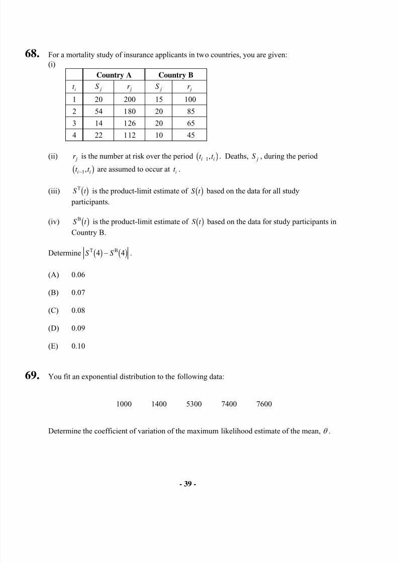
68. For a mortality study of insurance applicants in two countries, you are given:(i)
Country A Country B
t i jS jr jS jr
1 20 200 15 1002 54 180 20 85
3 14 126 20 65
4 22 112 10 45
(ii) jr is the number at risk over the period t t i i−1,b g . Deaths, jS , during the period
t t i i−1,b g are assumed to occur at t i .
(iii) S t Tb g is the product-limit estimate of S t b g based on the data for all study
participants.
(iv) S t Bb g is the product-limit estimate of S t b g based on the data for study participants in
Country B.
Determine S S T B4 4b g b g− .
(A) 0.06
(B) 0.07
(C) 0.08
(D) 0.09
(E) 0.10
69. You fit an exponential distribution to the following data:
1000 1400 5300 7400 7600
Determine the coefficient of variation of the maximum likelihood estimate of the mean, θ .
8/13/2019 Edu Exam c Sample Quest
http://slidepdf.com/reader/full/edu-exam-c-sample-quest 40/184
- 40 -
(A) 0.33
(B) 0.45
(C) 0.70
(D) 1.00
(E) 1.21
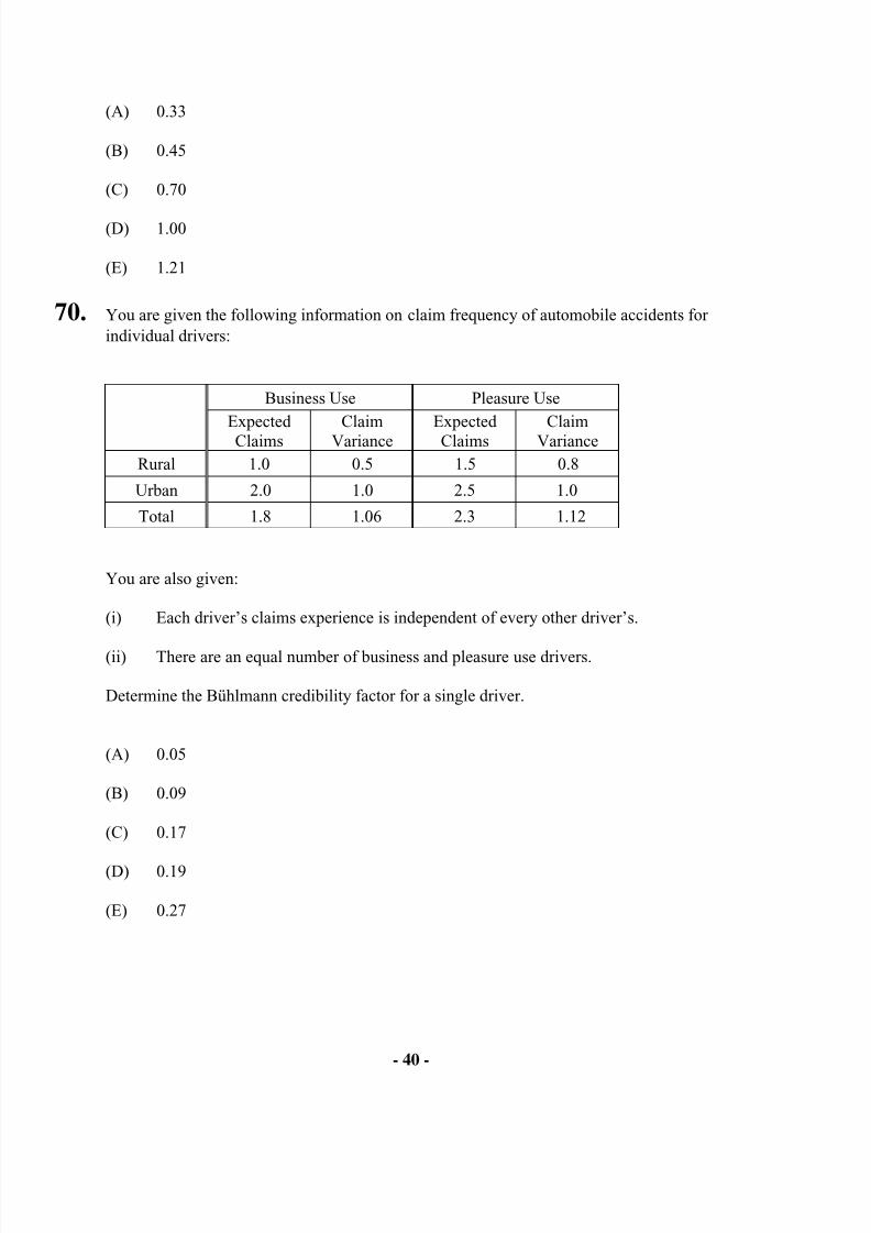
70. You are given the following information on claim frequency of automobile accidents forindividual drivers:
Business Use Pleasure Use
ExpectedClaims
ClaimVariance
ExpectedClaims
ClaimVariance
Rural 1.0 0.5 1.5 0.8
Urban 2.0 1.0 2.5 1.0
Total 1.8 1.06 2.3 1.12
You are also given:
(i) Each driver’s claims experience is independent of every other driver’s.
(ii) There are an equal number of business and pleasure use drivers.
Determine the Bühlmann credibility factor for a single driver.
(A) 0.05
(B) 0.09
(C) 0.17
(D) 0.19
(E) 0.27
8/13/2019 Edu Exam c Sample Quest
http://slidepdf.com/reader/full/edu-exam-c-sample-quest 41/184
- 41 -
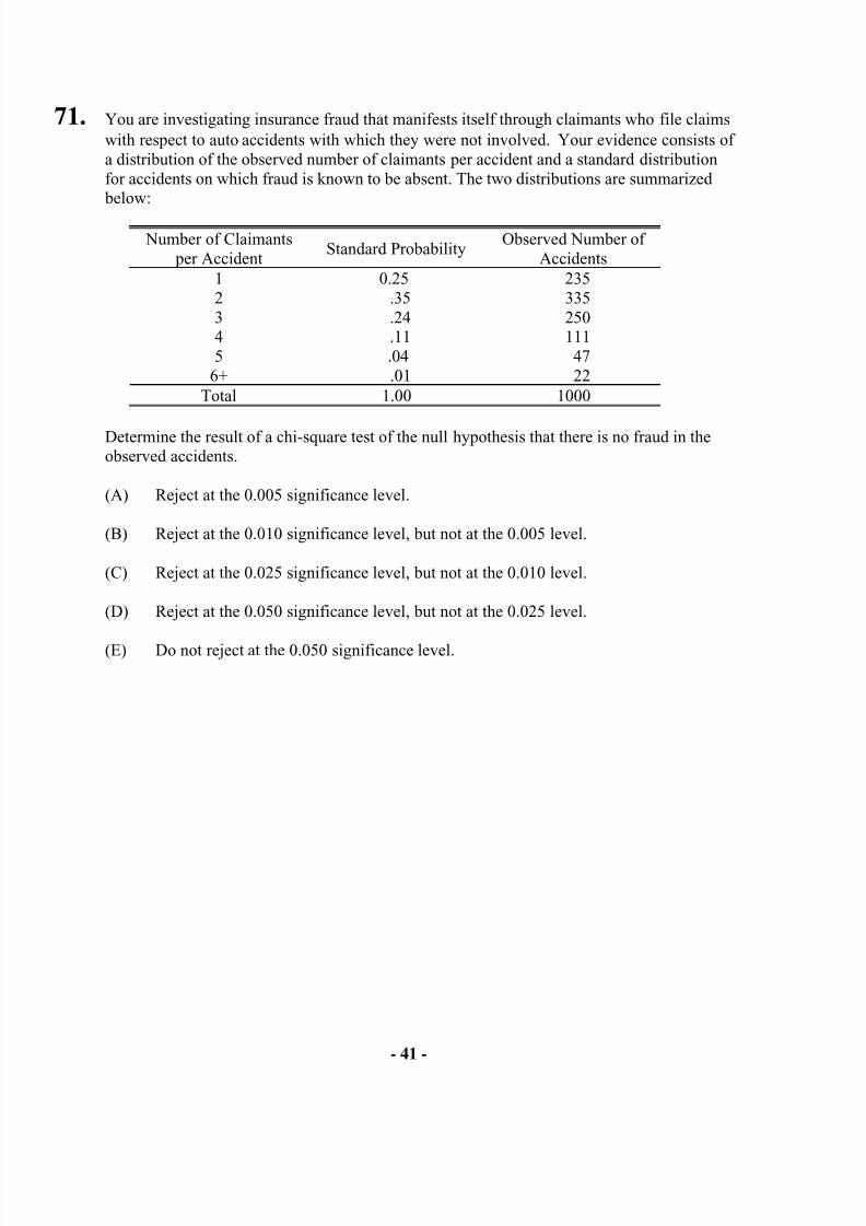
71. You are investigating insurance fraud that manifests itself through claimants who file claimswith respect to auto accidents with which they were not involved. Your evidence consists ofa distribution of the observed number of claimants per accident and a standard distributionfor accidents on which fraud is known to be absent. The two distributions are summarized below:
Number of Claimants per Accident
Standard ProbabilityObserved Number of
Accidents1 0.25 2352 .35 3353 .24 2504 .11 1115 .04 47
6+ .01 22Total 1.00 1000
Determine the result of a chi-square test of the null hypothesis that there is no fraud in theobserved accidents.
(A) Reject at the 0.005 significance level.
(B) Reject at the 0.010 significance level, but not at the 0.005 level.
(C) Reject at the 0.025 significance level, but not at the 0.010 level.
(D) Reject at the 0.050 significance level, but not at the 0.025 level.
(E) Do not reject at the 0.050 significance level.
8/13/2019 Edu Exam c Sample Quest
http://slidepdf.com/reader/full/edu-exam-c-sample-quest 42/184
- 42 -
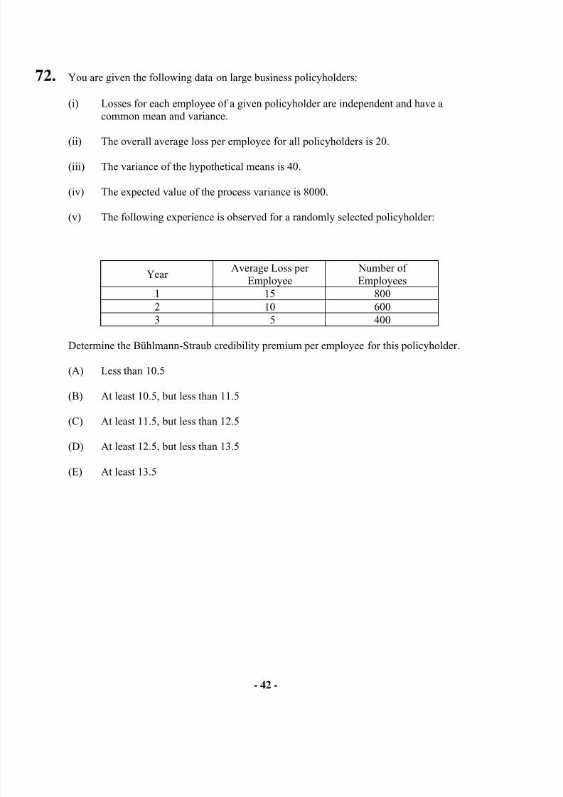
72. You are given the following data on large business policyholders:
(i) Losses for each employee of a given policyholder are independent and have acommon mean and variance.
(ii) The overall average loss per employee for all policyholders is 20.
(iii) The variance of the hypothetical means is 40.
(iv) The expected value of the process variance is 8000.
(v) The following experience is observed for a randomly selected policyholder:
Year
Average Loss per
Employee
Number of
Employees1 15 8002 10 6003 5 400
Determine the Bühlmann-Straub credibility premium per employee for this policyholder.
(A) Less than 10.5
(B) At least 10.5, but less than 11.5
(C) At least 11.5, but less than 12.5
(D) At least 12.5, but less than 13.5
(E) At least 13.5
8/13/2019 Edu Exam c Sample Quest
http://slidepdf.com/reader/full/edu-exam-c-sample-quest 43/184
- 43 -
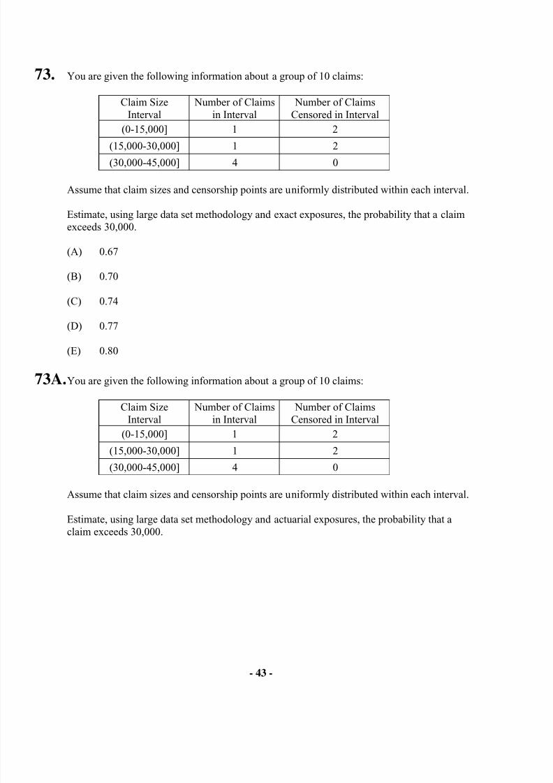
73. You are given the following information about a group of 10 claims:
Claim SizeInterval
Number of Claimsin Interval
Number of ClaimsCensored in Interval
(0-15,000] 1 2
(15,000-30,000] 1 2
(30,000-45,000] 4 0
Assume that claim sizes and censorship points are uniformly distributed within each interval.
Estimate, using large data set methodology and exact exposures, the probability that a claimexceeds 30,000.
(A) 0.67
(B) 0.70
(C) 0.74
(D) 0.77
(E) 0.80
73A.You are given the following information about a group of 10 claims:
Claim SizeInterval Number of Claimsin Interval Number of ClaimsCensored in Interval
(0-15,000] 1 2
(15,000-30,000] 1 2
(30,000-45,000] 4 0
Assume that claim sizes and censorship points are uniformly distributed within each interval.
Estimate, using large data set methodology and actuarial exposures, the probability that aclaim exceeds 30,000.
8/13/2019 Edu Exam c Sample Quest
http://slidepdf.com/reader/full/edu-exam-c-sample-quest 44/184
- 44 -
(A) 0.67
(B) 0.70
(C) 0.74
(D) 0.77
(E) 0.80
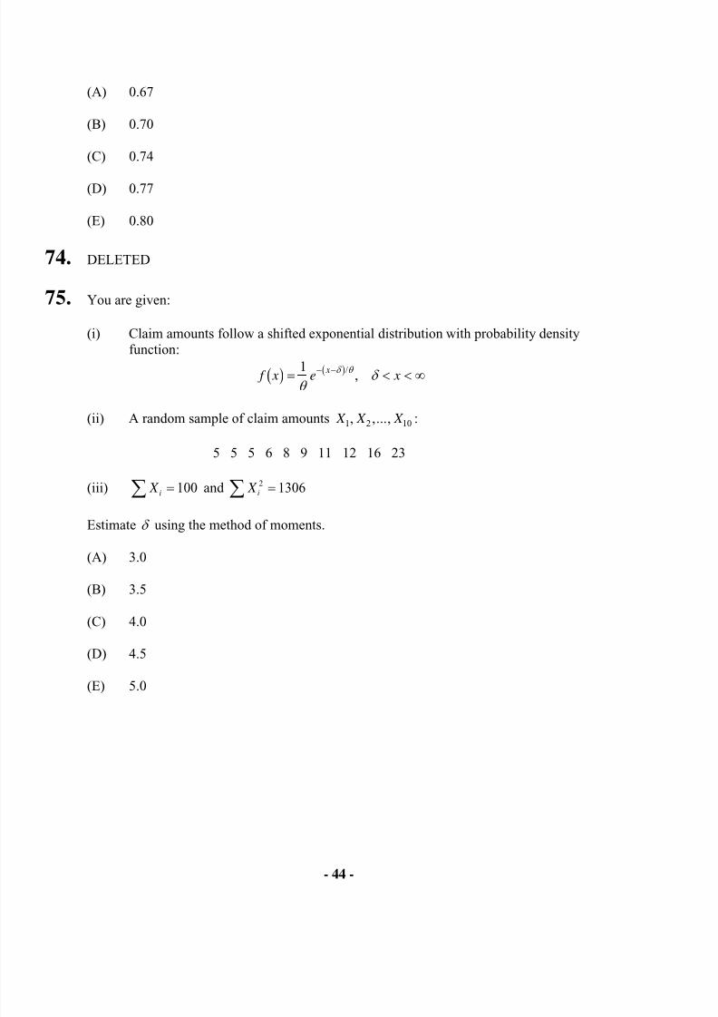
74. DELETED
75. You are given:
(i) Claim amounts follow a shifted exponential distribution with probability density
function: f x e x
xb g b g= < < ∞− −1
θ δ
δ θ / ,
(ii) A random sample of claim amounts X X X 1 2 10, ,..., :
5 5 5 6 8 9 11 12 16 23
(iii) X i∑ = 100 and X i2 1306∑ =
Estimate δ using the method of moments.
(A) 3.0
(B) 3.5
(C) 4.0
(D) 4.5
(E) 5.0
8/13/2019 Edu Exam c Sample Quest
http://slidepdf.com/reader/full/edu-exam-c-sample-quest 45/184
- 45 -
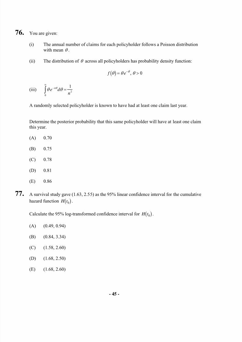
76. You are given:
(i) The annual number of claims for each policyholder follows a Poisson distributionwith mean θ .
(ii) The distribution of θ across all policyholders has probability density function:
f eθ θ θ θ b g = >− , 0
(iii) θ θ θ e d n
n−∞
z =0
2
1
A randomly selected policyholder is known to have had at least one claim last year.
Determine the posterior probability that this same policyholder will have at least one claimthis year.
(A) 0.70
(B) 0.75
(C) 0.78
(D) 0.81
(E) 0.86
77. A survival study gave (1.63, 2.55) as the 95% linear confidence interval for the cumulative
hazard function H t 0b g .
Calculate the 95% log-transformed confidence interval for H t 0b g .
(A) (0.49, 0.94)
(B) (0.84, 3.34)
(C) (1.58, 2.60)
(D) (1.68, 2.50)
(E) (1.68, 2.60)

8/13/2019 Edu Exam c Sample Quest
http://slidepdf.com/reader/full/edu-exam-c-sample-quest 46/184
- 46 -
8/13/2019 Edu Exam c Sample Quest
http://slidepdf.com/reader/full/edu-exam-c-sample-quest 47/184
- 47 -
78. You are given:
(i) Claim size, X , has mean µ and variance 500.
(ii) The random variable µ has a mean of 1000 and variance of 50.
(iii) The following three claims were observed: 750, 1075, 2000
Calculate the expected size of the next claim using Bühlmann credibility.
(A) 1025
(B) 1063
(C) 1115
(D) 1181
(E) 1266
79. Losses come from a mixture of an exponential distribution with mean 100 with probability p and an exponential distribution with mean 10,000 with probability 1− p .
Losses of 100 and 2000 are observed.
Determine the likelihood function of p.
(A) pe p e pe p e− − − −−F
H G I
K J −F
H G I
K J 1 0 01 20 0 2
100
1
10 000 100
1
10 000.
,. .
,
. .b g b g
(B) pe p e pe p e− − − −−F
H G I
K J +
−F H G
I K J
1 0 01 20 0 2
100
1
10 000 100
1
10 000.
,.
,
. .b g b g
(C) pe p e pe p e− − − −
+ −F
H G
I
K J +
−F
H G
I
K J
1 0 01 20 0 2
100
1
10 000 100
1
10 000
b g b g. .
,
.
,
(D) pe p e pe p e− − − −
+ −F
H G I
K J + +
−F H G
I K J
1 0 01 20 0 2
100
1
10 000 100
1
10 000
b g b g. .
, ,
8/13/2019 Edu Exam c Sample Quest
http://slidepdf.com/reader/full/edu-exam-c-sample-quest 48/184
- 48 -
(E) p e e
p e e
.,
.,
. .− − − −
+F H G
I K J
+ − +F H G
I K J
1 0 01 20 0 2
100 10 0001
100 10 000b g
80. DELETED
81. You wish to simulate a value, Y , from a two point mixture.
With probability 0.3, Y is exponentially distributed with mean 0.5. With probability 0.7, Y
is uniformly distributed on −3 3, . You simulate the mixing variable where low values
correspond to the exponential distribution. Then you simulate the value of Y , where low
random numbers correspond to low values of Y . Your uniform random numbers from 0 1,
are 0.25 and 0.69 in that order.
Calculate the simulated value of Y .
(A) 0.19
(B) 0.38
(C) 0.59
(D) 0.77
(E) 0.95
8/13/2019 Edu Exam c Sample Quest
http://slidepdf.com/reader/full/edu-exam-c-sample-quest 49/184
- 49 -
82. N is the random variable for the number of accidents in a single year. N follows thedistribution:
1Pr( ) 0.9(0.1)n N n = = , n = 1, 2,…
i X is the random variable for the claim amount of the ith accident. i X follows the
distribution:
0.010.01 , 0,i xi ig x e x i= > = 1, 2,…
Let U and 1 2, , ...V V be independent random variables following the uniform distribution on
(0, 1). You use the inverse transformation method with U to simulate N and iV to simulate
i X with small values of random numbers corresponding to small values of N and i X .
You are given the following random numbers for the first simulation:
u 1v 2v 3v 4v
0.05 0.30 0.22 0.52 0.46
Calculate the total amount of claims during the year for the first simulation.
(A) 0
(B) 36
(C) 72
(D) 108
(E) 144
8/13/2019 Edu Exam c Sample Quest
http://slidepdf.com/reader/full/edu-exam-c-sample-quest 50/184
- 50 -
83. You are the consulting actuary to a group of venture capitalists financing a search for pirategold.
It’s a risky undertaking: with probability 0.80, no treasure will be found, and thus theoutcome is 0.
The rewards are high: with probability 0.20 treasure will be found. The outcome, if treasureis found, is uniformly distributed on [1000, 5000].
You use the inverse transformation method to simulate the outcome, where large randomnumbers from the uniform distribution on [0, 1] correspond to large outcomes.
Your random numbers for the first two trials are 0.75 and 0.85.
Calculate the average of the outcomes of these first two trials.
(A) 0
(B) 1000
(C) 2000
(D) 3000
(E) 4000
84. A health plan implements an incentive to physicians to control hospitalization under whichthe physicians will be paid a bonus B equal to c times the amount by which total hospital
claims are under 400 0 1c ≤ .
The effect the incentive plan will have on underlying hospital claims is modeled by assumingthat the new total hospital claims will follow a two-parameter Pareto distribution with 2α = and 300θ = .
E( ) 100 B =
Calculate c.
8/13/2019 Edu Exam c Sample Quest
http://slidepdf.com/reader/full/edu-exam-c-sample-quest 51/184
- 51 -
(A) 0.44
(B) 0.48
(C) 0.52
(D) 0.56
(E) 0.60
85. Computer maintenance costs for a department are modeled as follows:
(i) The distribution of the number of maintenance calls each machine will need in a yearis Poisson with mean 3.
(ii) The cost for a maintenance call has mean 80 and standard deviation 200.
(iii) The number of maintenance calls and the costs of the maintenance calls are allmutually independent.
The department must buy a maintenance contract to cover repairs if there is at least a 10% probability that aggregate maintenance costs in a given year will exceed 120% of theexpected costs.
Using the normal approximation for the distribution of the aggregate maintenance costs,calculate the minimum number of computers needed to avoid purchasing a maintenancecontract.
(A) 80
(B) 90
(C) 100
(D) 110
(E) 120
8/13/2019 Edu Exam c Sample Quest
http://slidepdf.com/reader/full/edu-exam-c-sample-quest 52/184
- 52 -
86. Aggregate losses for a portfolio of policies are modeled as follows:
(i) The number of losses before any coverage modifications follows a Poissondistribution with mean λ .
(ii) The severity of each loss before any coverage modifications is uniformly distributed between 0 and b.
The insurer would like to model the impact of imposing an ordinary deductible,
0d d b< , on each loss and reimbursing only a percentage, c 0 1c ≤ , of each loss in
excess of the deductible.
It is assumed that the coverage modifications will not affect the loss distribution.The insurer models its claims with modified frequency and severity distributions. The
modified claim amount is uniformly distributed on the interval ( )0,c b d − .
Determine the mean of the modified frequency distribution.
(A) λ
(B) cλ
(C) d
bλ
(D) b d
bλ
(E) b d
cb
λ
8/13/2019 Edu Exam c Sample Quest
http://slidepdf.com/reader/full/edu-exam-c-sample-quest 53/184
- 53 -
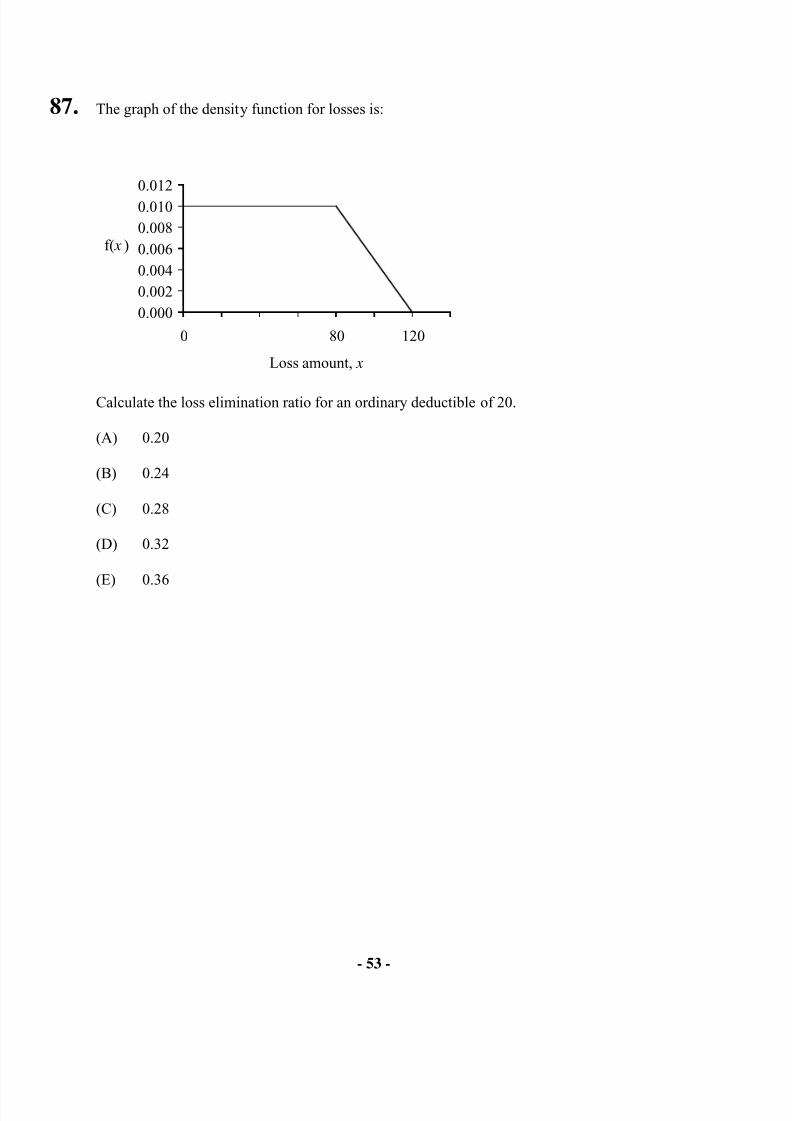
87. The graph of the density function for losses is:
0.000
0.002
0.004
0.006
0.008
0.010
0.012
0 80 120
Loss amount, x
f( x )
Calculate the loss elimination ratio for an ordinary deductible of 20.
(A) 0.20
(B) 0.24
(C) 0.28
(D) 0.32
(E) 0.36
8/13/2019 Edu Exam c Sample Quest
http://slidepdf.com/reader/full/edu-exam-c-sample-quest 54/184
- 54 -
88. A towing company provides all towing services to members of the City Automobile Club.You are given:
Towing Distance Towing Cost Frequency
0-9.99 miles 80 50%
10-29.99 miles 100 40%30+ miles 160 10%
(i) The automobile owner must pay 10% of the cost and the remainder is paid by the CityAutomobile Club.
(ii) The number of towings has a Poisson distribution with mean of 1000 per year.
(iii) The number of towings and the costs of individual towings are all mutuallyindependent.
Using the normal approximation for the distribution of aggregate towing costs, calculate the probability that the City Automobile Club pays more than 90,000 in any given year.
(A) 3%
(B) 10%
(C) 50%
(D) 90%
(E) 97%
89. You are given:(i) Losses follow an exponential distribution with the same mean in all years.
(ii) The loss elimination ratio this year is 70%.
(iii) The ordinary deductible for the coming year is 4/3 of the current deductible.
Compute the loss elimination ratio for the coming year.
(A) 70%
(B) 75%
(C) 80%
(D) 85%
8/13/2019 Edu Exam c Sample Quest
http://slidepdf.com/reader/full/edu-exam-c-sample-quest 55/184
- 55 -
(E) 90%
90. Actuaries have modeled auto windshield claim frequencies. They have concluded that thenumber of windshield claims filed per year per driver follows the Poisson distribution with parameter λ , where λ follows the gamma distribution with mean 3 and variance 3.
Calculate the probability that a driver selected at random will file no more than 1 windshieldclaim next year.
(A) 0.15
(B) 0.19
(C) 0.20
(D) 0.24
(E) 0.31
91. The number of auto vandalism claims reported per month at Sunny Daze Insurance Company(SDIC) has mean 110 and variance 750. Individual losses have mean 1101 and standarddeviation 70. The number of claims and the amounts of individual losses are independent.
Using the normal approximation, calculate the probability that SDIC’s aggregate autovandalism losses reported for a month will be less than 100,000.
(A) 0.24
(B) 0.31
(C) 0.36
(D) 0.39
(E) 0.49
92. Prescription drug losses, S , are modeled assuming the number of claims has a geometricdistribution with mean 4, and the amount of each prescription is 40.

8/13/2019 Edu Exam c Sample Quest
http://slidepdf.com/reader/full/edu-exam-c-sample-quest 56/184
- 56 -
Calculate E S −+
100b g .
8/13/2019 Edu Exam c Sample Quest
http://slidepdf.com/reader/full/edu-exam-c-sample-quest 57/184
- 57 -
(A) 60
(B) 82
(C) 92
(D) 114
(E) 146
93. At the beginning of each round of a game of chance the player pays 12.5. The player thenrolls one die with outcome N . The player then rolls N dice and wins an amount equal to thetotal of the numbers showing on the N dice. All dice have 6 sides and are fair.
Using the normal approximation, calculate the probability that a player starting with 15,000will have at least 15,000 after 1000 rounds.
(A) 0.01
(B) 0.04
(C) 0.06
(D) 0.09
(E) 0.12
94. X is a discrete random variable with a probability function which is a member of the (a,b,0)class of distributions.
You are given:(i) P X P X ( = ) = ( = ) = .0 1 0 25
(ii) P X ( = ) = .2 0 1875
Calculate P X = 3b g .
8/13/2019 Edu Exam c Sample Quest
http://slidepdf.com/reader/full/edu-exam-c-sample-quest 58/184
- 58 -
(A) 0.120
(B) 0.125
(C) 0.130
(D) 0.135
(E) 0.140
95. The number of claims in a period has a geometric distribution with mean 4. The amount of
each claim X follows P X x= =b g 0 25. , x = 12 3 4, , , . The number of claims and the claim
amounts are independent. S is the aggregate claim amount in the period.
Calculate F s 3b g .
(A) 0.27
(B) 0.29
(C) 0.31
(D) 0.33
(E) 0.35
96. Insurance agent Hunt N. Quotum will receive no annual bonus if the ratio of incurred lossesto earned premiums for his book of business is 60% or more for the year. If the ratio is lessthan 60%, Hunt’s bonus will be a percentage of his earned premium equal to 15% of thedifference between his ratio and 60%. Hunt’s annual earned premium is 800,000.
Incurred losses are distributed according to the Pareto distribution, with θ = 500 000, andα = 2 .
Calculate the expected value of Hunt’s bonus.
(A) 13,000
(B) 17,000
(C) 24,000
(D) 29,000
(E) 35,000
8/13/2019 Edu Exam c Sample Quest
http://slidepdf.com/reader/full/edu-exam-c-sample-quest 59/184
- 59 -
97. A group dental policy has a negative binomial claim count distribution with mean 300 andvariance 800.
Ground-up severity is given by the following table:
Severity Probability
40 0.25
80 0.25
120 0.25
200 0.25
You expect severity to increase 50% with no change in frequency. You decide to impose a per claim deductible of 100.
Calculate the expected total claim payment after these changes.
(A) Less than 18,000
(B) At least 18,000, but less than 20,000
(C) At least 20,000, but less than 22,000
(D) At least 22,000, but less than 24,000
(E) At least 24,000
98. You own a fancy light bulb factory. Your workforce is a bit clumsy – they keep dropping boxes of light bulbs. The boxes have varying numbers of light bulbs in them, and whendropped, the entire box is destroyed.
You are given:
Expected number of boxes dropped per month: 50
Variance of the number of boxes dropped per month: 100
Expected value per box: 200
Variance of the value per box: 400
You pay your employees a bonus if the value of light bulbs destroyed in a month is less than8000.
Assuming independence and using the normal approximation, calculate the probability thatyou will pay your employees a bonus next month.
8/13/2019 Edu Exam c Sample Quest
http://slidepdf.com/reader/full/edu-exam-c-sample-quest 60/184
8/13/2019 Edu Exam c Sample Quest
http://slidepdf.com/reader/full/edu-exam-c-sample-quest 61/184
- 61 -
(D) 205
(E) 240
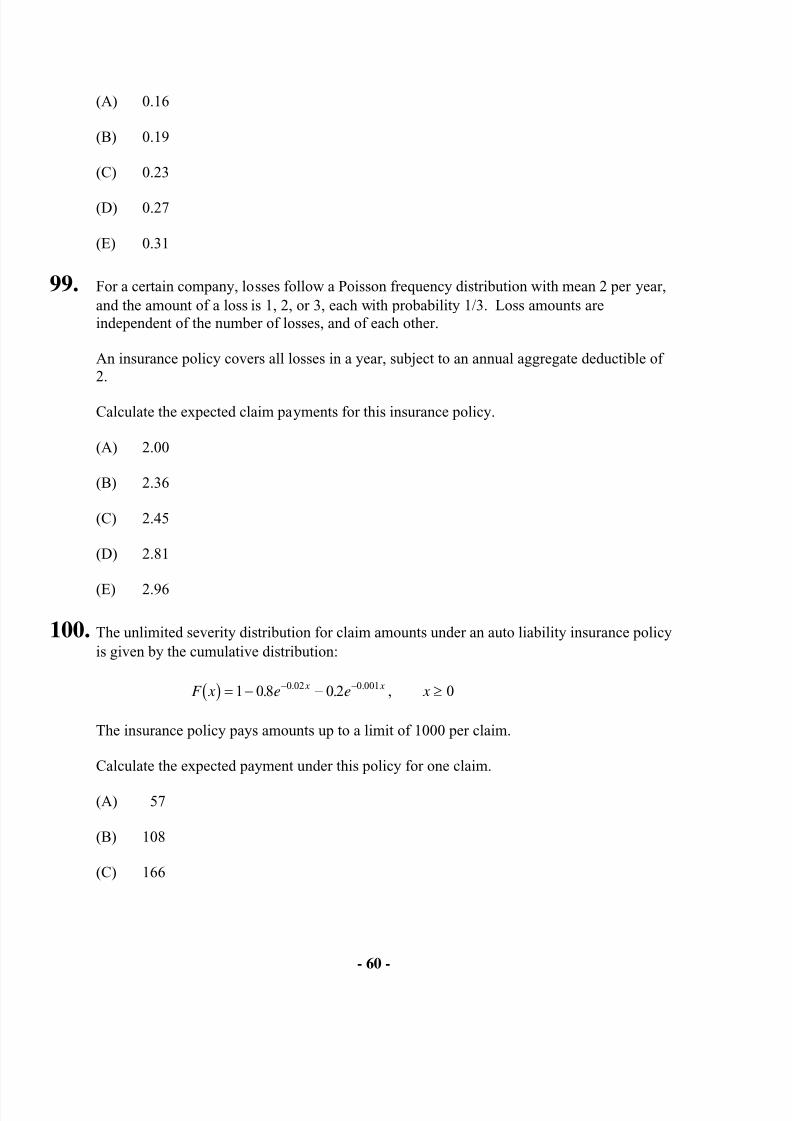
101. The random variable for a loss, X , has the following characteristics:
x F xb g E X x∧b g
0 0.0 0
100 0.2 91
200 0.6 153
1000 1.0 331
Calculate the mean excess loss for a deductible of 100.
(A) 250
(B) 300
(C) 350
(D) 400
(E) 450
102. WidgetsRUs owns two factories. It buys insurance to protect itself against major repaircosts. Profit equals revenues, less the sum of insurance premiums, retained major repaircosts, and all other expenses. WidgetsRUs will pay a dividend equal to the profit, if it is positive.
You are given:
(i) Combined revenue for the two factories is 3.
(ii) Major repair costs at the factories are independent.
(iii) The distribution of major repair costs for each factory is
k Prob (k )
0 0.41 0.3
2 0.2
3 0.1
(iv) At each factory, the insurance policy pays the major repair costs in excess of thatfactory’s ordinary deductible of 1. The insurance premium is 110% of the expected
8/13/2019 Edu Exam c Sample Quest
http://slidepdf.com/reader/full/edu-exam-c-sample-quest 62/184
- 62 -
claims.
(v) All other expenses are 15% of revenues.
Calculate the expected dividend.
(A) 0.43
(B) 0.47
(C) 0.51
(D) 0.55
(E) 0.59
103. For watches produced by a certain manufacturer:(i) Lifetimes follow a single-parameter Pareto distribution with α > 1 and θ = 4.
(ii) The expected lifetime of a watch is 8 years.
Calculate the probability that the lifetime of a watch is at least 6 years.
(A) 0.44
(B) 0.50
(C) 0.56
(D) 0.61
(E) 0.67
104. Glen is practicing his simulation skills.He generates 1000 values of the random variable X as follows:(i) He generates the observed value λ from the gamma distribution with α = 2 and
θ =1
(hence with mean 2 and variance 2).
(ii) He then generates x from the Poisson distribution with mean λ .
(iii) He repeats the process 999 more times: first generating a value λ , then generating x from the Poisson distribution with mean λ .
(iv) The repetitions are mutually independent.

8/13/2019 Edu Exam c Sample Quest
http://slidepdf.com/reader/full/edu-exam-c-sample-quest 63/184
- 63 -
Calculate the expected number of times that his simulated value of X is 3.
8/13/2019 Edu Exam c Sample Quest
http://slidepdf.com/reader/full/edu-exam-c-sample-quest 64/184
- 64 -
(A) 75
(B) 100
(C) 125
(D) 150
(E) 175
105. An actuary for an automobile insurance company determines that the distribution of theannual number of claims for an insured chosen at random is modeled by the negative binomial distribution with mean 0.2 and variance 0.4.
The number of claims for each individual insured has a Poisson distribution and the means ofthese Poisson distributions are gamma distributed over the population of insureds.
Calculate the variance of this gamma distribution.
(A) 0.20
(B) 0.25
(C) 0.30
(D) 0.35
(E) 0.40
106. A dam is proposed for a river which is currently used for salmon breeding. You havemodeled:
(i) For each hour the dam is opened the number of salmon that will pass through andreach the breeding grounds has a distribution with mean 100 and variance 900.
(ii) The number of eggs released by each salmon has a distribution with mean of 5 andvariance of 5.
(iii) The number of salmon going through the dam each hour it is open and the numbers ofeggs released by the salmon are independent.
Using the normal approximation for the aggregate number of eggs released, determine theleast number of whole hours the dam should be left open so the probability that 10,000 eggswill be released is greater than 95%.
8/13/2019 Edu Exam c Sample Quest
http://slidepdf.com/reader/full/edu-exam-c-sample-quest 65/184
- 65 -
(A) 20
(B) 23
(C) 26
(D) 29
(E) 32
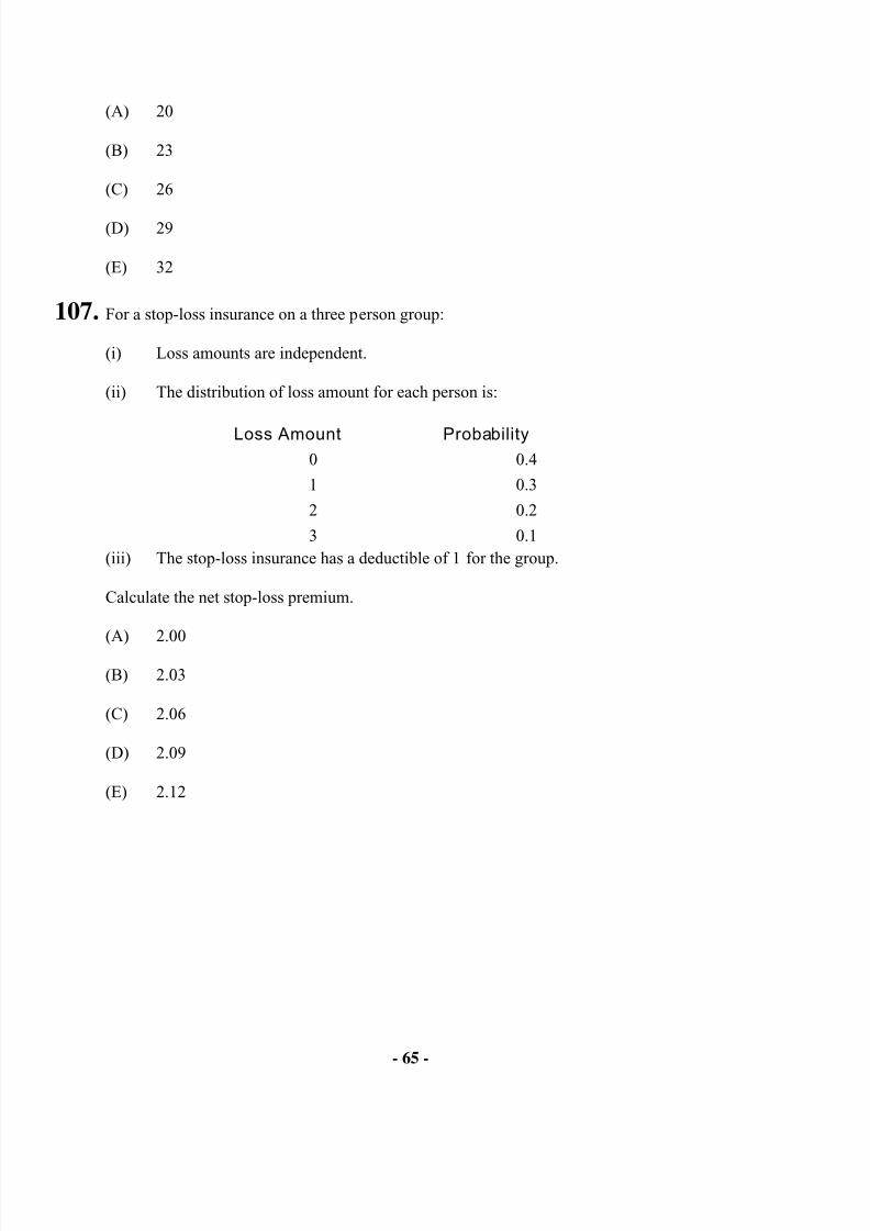
107. For a stop-loss insurance on a three person group:
(i) Loss amounts are independent.
(ii) The distribution of loss amount for each person is:
Loss Amount Probability
0 0.4
1 0.3
2 0.2
3 0.1
(iii) The stop-loss insurance has a deductible of 1 for the group.
Calculate the net stop-loss premium.
(A) 2.00
(B) 2.03
(C) 2.06
(D) 2.09
(E) 2.12
8/13/2019 Edu Exam c Sample Quest
http://slidepdf.com/reader/full/edu-exam-c-sample-quest 66/184
- 66 -
108. For a discrete probability distribution, you are given the recursion relation
p k k
p k b g b g= −2
1* , k = 1, 2,….
Determine p 4b g.
(A) 0.07
(B) 0.08
(C) 0.09
(D) 0.10
(E) 0.11
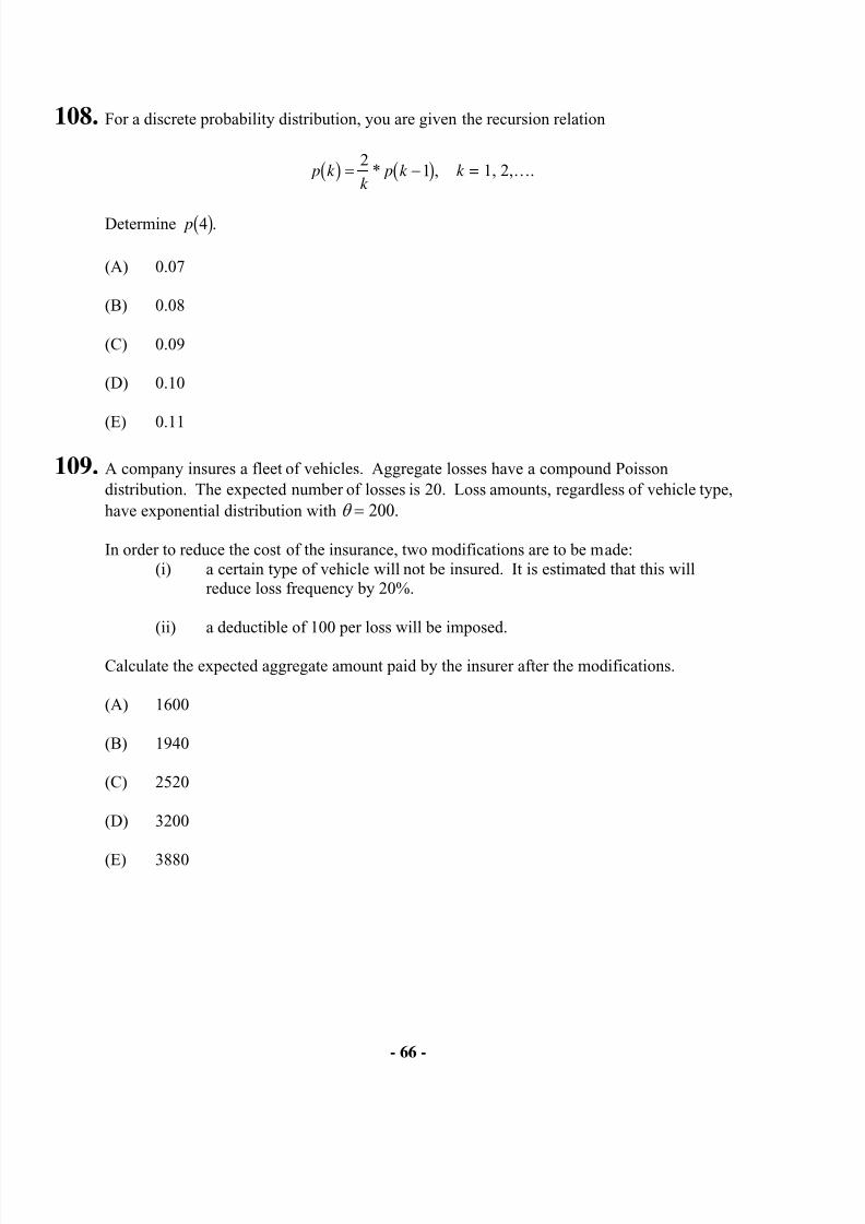
109. A company insures a fleet of vehicles. Aggregate losses have a compound Poissondistribution. The expected number of losses is 20. Loss amounts, regardless of vehicle type,have exponential distribution with θ = 200.
In order to reduce the cost of the insurance, two modifications are to be made:(i) a certain type of vehicle will not be insured. It is estimated that this will
reduce loss frequency by 20%.
(ii) a deductible of 100 per loss will be imposed.
Calculate the expected aggregate amount paid by the insurer after the modifications.
(A) 1600
(B) 1940
(C) 2520
(D) 3200
(E) 3880
8/13/2019 Edu Exam c Sample Quest
http://slidepdf.com/reader/full/edu-exam-c-sample-quest 67/184
- 67 -
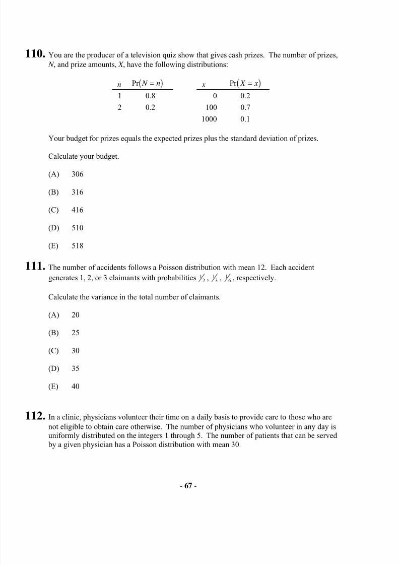
110. You are the producer of a television quiz show that gives cash prizes. The number of prizes, N , and prize amounts, X , have the following distributions:
n Pr N n=b g x Pr X x=b g
1 0.8 0 0.22 0.2 100 0.7
1000 0.1
Your budget for prizes equals the expected prizes plus the standard deviation of prizes.
Calculate your budget.
(A) 306
(B) 316
(C) 416
(D) 510
(E) 518
111. The number of accidents follows a Poisson distribution with mean 12. Each accident
generates 1, 2, or 3 claimants with probabilities 12 , 1
3 , 16 , respectively.
Calculate the variance in the total number of claimants.
(A) 20
(B) 25
(C) 30
(D) 35
(E) 40
112. In a clinic, physicians volunteer their time on a daily basis to provide care to those who arenot eligible to obtain care otherwise. The number of physicians who volunteer in any day isuniformly distributed on the integers 1 through 5. The number of patients that can be served by a given physician has a Poisson distribution with mean 30.
8/13/2019 Edu Exam c Sample Quest
http://slidepdf.com/reader/full/edu-exam-c-sample-quest 68/184
- 68 -
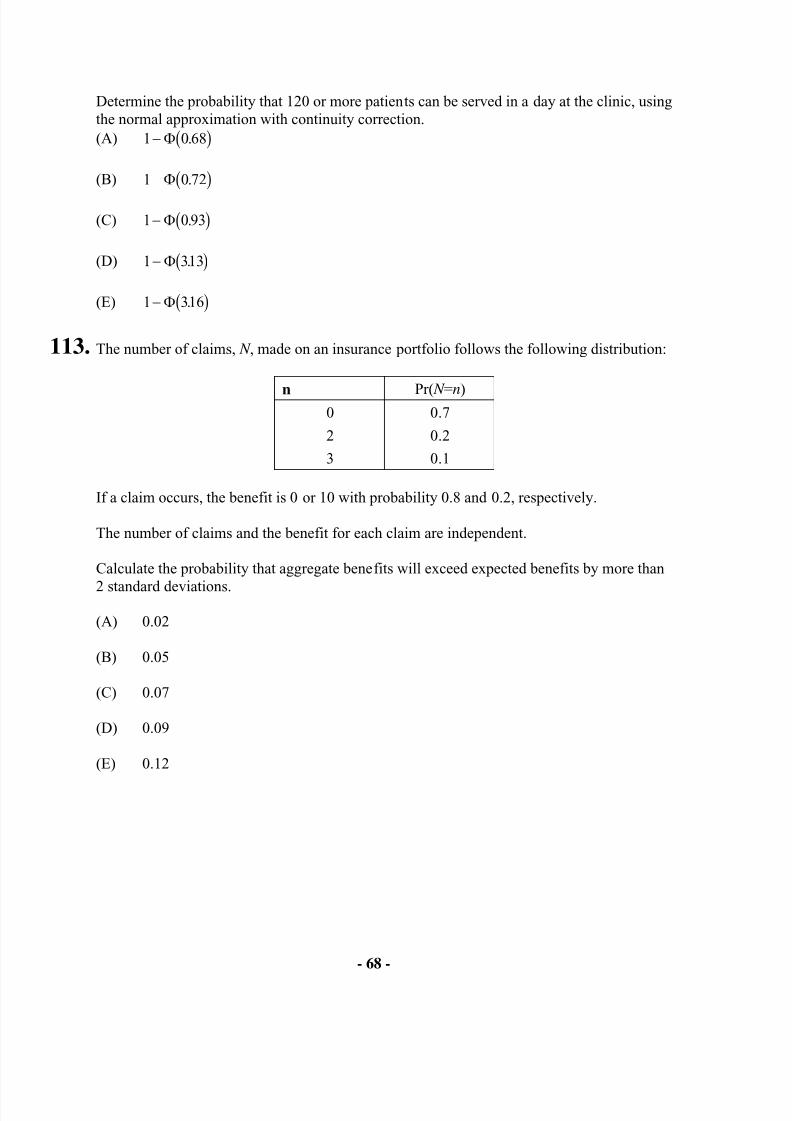
Determine the probability that 120 or more patients can be served in a day at the clinic, usingthe normal approximation with continuity correction.(A) 1 0 68− Φ .b g
(B) 1 0 72− Φ .b g
(C) 1 0 93− Φ .b g
(D) 1 313− Φ .b g
(E) 1 316− Φ .b g
113. The number of claims, N , made on an insurance portfolio follows the following distribution:
n Pr( N =n)0 0.7
2 0.2
3 0.1
If a claim occurs, the benefit is 0 or 10 with probability 0.8 and 0.2, respectively.
The number of claims and the benefit for each claim are independent.
Calculate the probability that aggregate benefits will exceed expected benefits by more than
2 standard deviations.
(A) 0.02
(B) 0.05
(C) 0.07
(D) 0.09
(E) 0.12
8/13/2019 Edu Exam c Sample Quest
http://slidepdf.com/reader/full/edu-exam-c-sample-quest 69/184
- 69 -
114. A claim count distribution can be expressed as a mixed Poisson distribution. The mean ofthe Poisson distribution is uniformly distributed over the interval [0,5].
Calculate the probability that there are 2 or more claims.
(A) 0.61
(B) 0.66
(C) 0.71
(D) 0.76
(E) 0.81
115.A claim severity distribution is exponential with mean 1000. An insurance company will paythe amount of each claim in excess of a deductible of 100.
Calculate the variance of the amount paid by the insurance company for one claim, includingthe possibility that the amount paid is 0.
(A) 810,000
(B) 860,000
(C) 900,000
(D) 990,000
(E) 1,000,000
116. Total hospital claims for a health plan were previously modeled by a two-parameter Paretodistribution with α = 2 and θ = 500 .
The health plan begins to provide financial incentives to physicians by paying a bonus of50% of the amount by which total hospital claims are less than 500. No bonus is paid if totalclaims exceed 500.
Total hospital claims for the health plan are now modeled by a new Pareto distribution withα = 2 and θ = K . The expected claims plus the expected bonus under the revised modelequals expected claims under the previous model.
Calculate K.
8/13/2019 Edu Exam c Sample Quest
http://slidepdf.com/reader/full/edu-exam-c-sample-quest 70/184
- 70 -
(A) 250
(B) 300
(C) 350
(D) 400
(E) 450
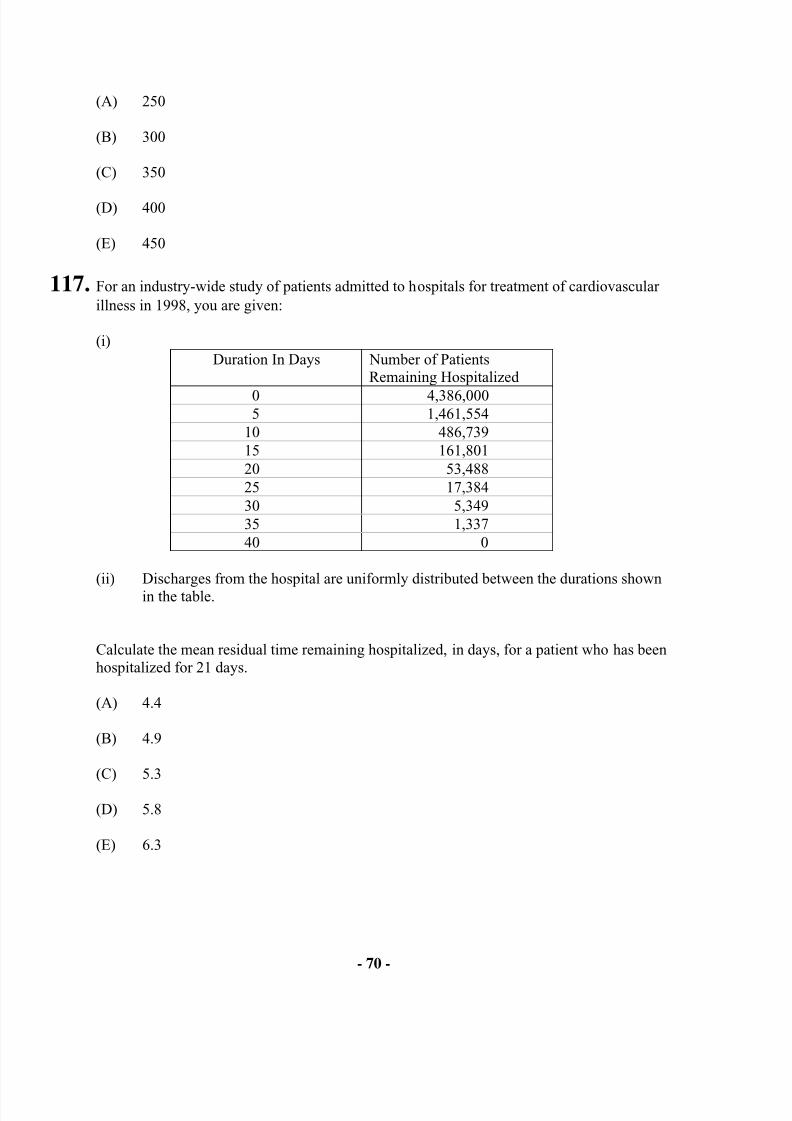
117. For an industry-wide study of patients admitted to hospitals for treatment of cardiovascularillness in 1998, you are given:
(i) Duration In Days Number of Patients
Remaining Hospitalized
0 4,386,0005 1,461,554
10 486,73915 161,80120 53,48825 17,38430 5,34935 1,33740 0
(ii) Discharges from the hospital are uniformly distributed between the durations shownin the table.
Calculate the mean residual time remaining hospitalized, in days, for a patient who has beenhospitalized for 21 days.
(A) 4.4
(B) 4.9
(C) 5.3
(D) 5.8
(E) 6.3
8/13/2019 Edu Exam c Sample Quest
http://slidepdf.com/reader/full/edu-exam-c-sample-quest 71/184
- 71 -
118. For an individual over 65:(i) The number of pharmacy claims is a Poisson random variable with mean 25.
(ii) The amount of each pharmacy claim is uniformly distributed between 5 and 95.
(iii) The amounts of the claims and the number of claims are mutually independent.
Determine the probability that aggregate claims for this individual will exceed 2000 using thenormal approximation.(A) 1 133− Φ .b g
(B) 1 166− Φ .b g
(C) 1 2 33− Φ .b g
(D) 1 2 66− Φ .b g
(E) 1 3 33− Φ .b g
119-120 Use the following information for questions 119 and 120.
An insurer has excess-of-loss reinsurance on auto insurance. You are given:
(i) Total expected losses in the year 2001 are 10,000,000.
(ii) In the year 2001 individual losses have a Pareto distribution with
F x x
xb g = −+
F H G
I K J >1
2000
20000
2
, .
(iii) Reinsurance will pay the excess of each loss over 3000.
(iv) Each year, the reinsurer is paid a ceded premium, C year , equal to 110% of the
expected losses covered by the reinsurance.
(v) Individual losses increase 5% each year due to inflation.
(vi) The frequency distribution does not change.
8/13/2019 Edu Exam c Sample Quest
http://slidepdf.com/reader/full/edu-exam-c-sample-quest 72/184
- 72 -
119. Calculate C 2001.
(A) 2,200,000
(B) 3,300,000
(C) 4,400,000
(D) 5,500,000
(E) 6,600,000
120. Calculate C C 2002 2001/ .
(A) 1.04
(B) 1.05
(C) 1.06
(D) 1.07
(E) 1.08
121. DELETED
8/13/2019 Edu Exam c Sample Quest
http://slidepdf.com/reader/full/edu-exam-c-sample-quest 73/184
- 73 -
122. You are simulating a compound claims distribution:
(i) The number of claims, N , is binomial with m = 3 and mean 1.8.
(ii) Claim amounts are uniformly distributed on { }1, 2, 3, 4, 5 .
(iii) Claim amounts are independent, and are independent of the number of claims.
(iv) You simulate the number of claims, N , then the amounts of each of those claims,
1 2, , , N X X X . Then you repeat another N , its claim amounts, and so on until you
have performed the desired number of simulations.
(v) When the simulated number of claims is 0, you do not simulate any claim amounts.
(vi) All simulations use the inverse transform method, with low random numbers
corresponding to few claims or small claim amounts.
(vii) Your random numbers from (0, 1) are 0.7, 0.1, 0.3, 0.1, 0.9, 0.5, 0.5, 0.7, 0.3, and 0.1.
Calculate the aggregate claim amount associated with your third simulated value of N .
(A) 3
(B) 5
(C) 7
(D) 9
(E) 11
8/13/2019 Edu Exam c Sample Quest
http://slidepdf.com/reader/full/edu-exam-c-sample-quest 74/184
- 74 -
123. Annual prescription drug costs are modeled by a two-parameter Pareto distribution with2000θ = and 2α = .
A prescription drug plan pays annual drug costs for an insured member subject to thefollowing provisions:
(i) The insured pays 100% of costs up to the ordinary annual deductible of 250.
(ii) The insured then pays 25% of the costs between 250 and 2250.
(iii) The insured pays 100% of the costs above 2250 until the insured has paid 3600 intotal.
(iv) The insured then pays 5% of the remaining costs.
Determine the expected annual plan payment.
(A) 1120
(B) 1140
(C) 1160
(D) 1180
(E) 1200
124. For a tyrannosaur with a taste for scientists:
(i) The number of scientists eaten has a binomial distribution with q = 0.6 and m = 8.
(ii) The number of calories of a scientist is uniformly distributed on (7000, 9000).
(iii) The numbers of calories of scientists eaten are independent, and are independent ofthe number of scientists eaten.
Calculate the probability that two or more scientists are eaten and exactly two of those eatenhave at least 8000 calories each.
8/13/2019 Edu Exam c Sample Quest
http://slidepdf.com/reader/full/edu-exam-c-sample-quest 75/184
- 75 -
(A) 0.23
(B) 0.25
(C) 0.27
(D) 0.30
(E) 0.35
125. Two types of insurance claims are made to an insurance company. For each type, thenumber of claims follows a Poisson distribution and the amount of each claim is uniformlydistributed as follows:
Type of Claim Poisson Parameter λ for Number of Claims in one
year
Range of Each ClaimAmount
I 12 (0, 1)
II 4 (0, 5)
The numbers of claims of the two types are independent and the claim amounts and claimnumbers are independent.
Calculate the normal approximation to the probability that the total of claim amounts in oneyear exceeds 18.
(A) 0.37
(B) 0.39
(C) 0.41
(D) 0.43
(E) 0.45
126. The number of annual losses has a Poisson distribution with a mean of 5. The size of eachloss has a two-parameter Pareto distribution with 10θ = and 2.5α = . An insurance for thelosses has an ordinary deductible of 5 per loss.
Calculate the expected value of the aggregate annual payments for this insurance.
8/13/2019 Edu Exam c Sample Quest
http://slidepdf.com/reader/full/edu-exam-c-sample-quest 76/184
- 76 -
(A) 8
(B) 13
(C) 18
(D) 23
(E) 28
127. Losses in 2003 follow a two-parameter Pareto distribution with α = 2 and θ = 5. Losses in2004 are uniformly 20% higher than in 2003. An insurance covers each loss subject to anordinary deductible of 10.
Calculate the Loss Elimination Ratio in 2004.
(A) 5/9
(B) 5/8
(C) 2/3
(D) 3/4
(E) 4/5
128. DELETED
129. DELETED
130. Bob is a carnival operator of a game in which a player receives a prize worth 2 N W = if the player has N successes, N = 0, 1, 2, 3,… Bob models the probability of success for a playeras follows:
(i) N has a Poisson distribution with mean Λ .
(ii) Λ has a uniform distribution on the interval (0, 4).
Calculate [ ]E W .
8/13/2019 Edu Exam c Sample Quest
http://slidepdf.com/reader/full/edu-exam-c-sample-quest 77/184
- 77 -
(A) 5
(B) 7
(C) 9
(D) 11
(E) 13
131. You are simulating the gain/loss from insurance where:
(i) Claim occurrences follow a Poisson process with 2 / 3λ = per year.
(ii) Each claim amount is 1, 2 or 3 with (1) 0.25, (2) 0.25, and (3) 0.50 p p p= = = .
(iii) Claim occurrences and amounts are independent.
(iv) The annual premium equals expected annual claims plus 1.8 times the standarddeviation of annual claims.
(v) i = 0
You use 0.25, 0.40, 0.60, and 0.80 from the unit interval and the inversion method tosimulate time between claims.
You use 0.30, 0.60, 0.20, and 0.70 from the unit interval and the inversion method to
simulate claim size.
Calculate the gain or loss from the insurer’s viewpoint during the first 2 years from thissimulation.
(A) loss of 5
(B) loss of 4
(C) 0
(D) gain of 4
(E) gain of 5
8/13/2019 Edu Exam c Sample Quest
http://slidepdf.com/reader/full/edu-exam-c-sample-quest 78/184
8/13/2019 Edu Exam c Sample Quest
http://slidepdf.com/reader/full/edu-exam-c-sample-quest 79/184
- 79 -
(A) 0.33
(B) 0.50
(C) 1.00
(D) 1.33
(E) 1.50
134. You are given the following random sample of 13 claim amounts:
99 133 175 216 250 277 651 698 735 745 791 906 947
Determine the smoothed empirical estimate of the 35th percentile.
(A) 219.4
(B) 231.3
(C) 234.7
(D) 246.6
(E) 256.8
8/13/2019 Edu Exam c Sample Quest
http://slidepdf.com/reader/full/edu-exam-c-sample-quest 80/184
- 80 -
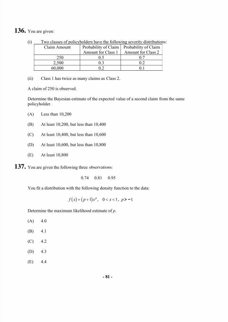
135. For observation i of a survival study:
• d i is the left truncation point
• xi is the observed value if not right censored
• ui is the observed value if right censored
You are given:
Observation (i) id i x iu
1 0 0.9 − 2 0 − 1.23 0 1.5 − 4 0 − 1.5
5 0 − 1.66 0 1.7 − 7 0 − 1.78 1.3 2.1 − 9 1.5 2.1 − 10 1.6 − 2.3
Determine the Kaplan-Meier Product-Limit estimate, 10S (1.6).
(A) Less than 0.55
(B) At least 0.55, but less than 0.60
(C) At least 0.60, but less than 0.65
(D) At least 0.65, but less than 0.70
(E) At least 0.70
8/13/2019 Edu Exam c Sample Quest
http://slidepdf.com/reader/full/edu-exam-c-sample-quest 81/184
8/13/2019 Edu Exam c Sample Quest
http://slidepdf.com/reader/full/edu-exam-c-sample-quest 82/184
- 82 -
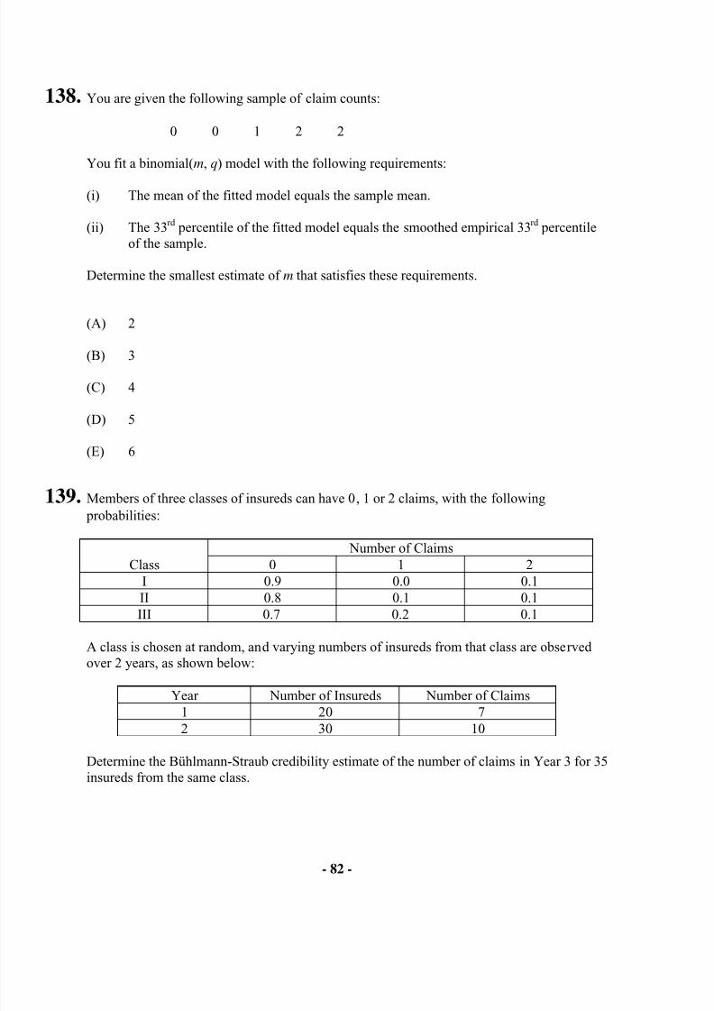
138. You are given the following sample of claim counts:
0 0 1 2 2
You fit a binomial(m, q) model with the following requirements:
(i) The mean of the fitted model equals the sample mean.
(ii) The 33rd percentile of the fitted model equals the smoothed empirical 33rd percentileof the sample.
Determine the smallest estimate of m that satisfies these requirements.
(A) 2
(B) 3
(C) 4
(D) 5
(E) 6
139. Members of three classes of insureds can have 0, 1 or 2 claims, with the following probabilities:
Number of ClaimsClass 0 1 2
I 0.9 0.0 0.1II 0.8 0.1 0.1III 0.7 0.2 0.1
A class is chosen at random, and varying numbers of insureds from that class are observedover 2 years, as shown below:
Year Number of Insureds Number of Claims
1 20 72 30 10
Determine the Bühlmann-Straub credibility estimate of the number of claims in Year 3 for 35insureds from the same class.
8/13/2019 Edu Exam c Sample Quest
http://slidepdf.com/reader/full/edu-exam-c-sample-quest 83/184
- 83 -
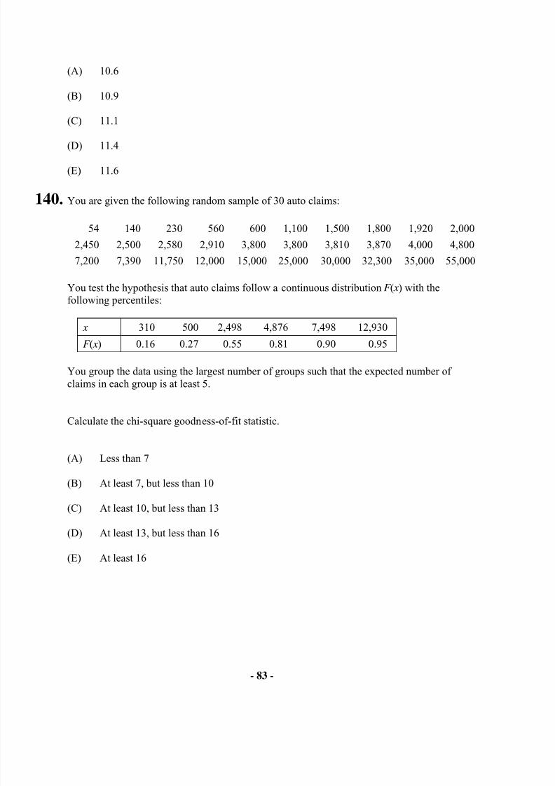
(A) 10.6
(B) 10.9
(C) 11.1
(D) 11.4
(E) 11.6
140. You are given the following random sample of 30 auto claims:
54 140 230 560 600 1,100 1,500 1,800 1,920 2,000
2,450 2,500 2,580 2,910 3,800 3,800 3,810 3,870 4,000 4,800
7,200 7,390 11,750 12,000 15,000 25,000 30,000 32,300 35,000 55,000
You test the hypothesis that auto claims follow a continuous distribution F ( x) with thefollowing percentiles:
x 310 500 2,498 4,876 7,498 12,930
F ( x) 0.16 0.27 0.55 0.81 0.90 0.95
You group the data using the largest number of groups such that the expected number ofclaims in each group is at least 5.
Calculate the chi-square goodness-of-fit statistic.
(A) Less than 7
(B) At least 7, but less than 10
(C) At least 10, but less than 13
(D) At least 13, but less than 16
(E) At least 16
8/13/2019 Edu Exam c Sample Quest
http://slidepdf.com/reader/full/edu-exam-c-sample-quest 84/184
- 84 -
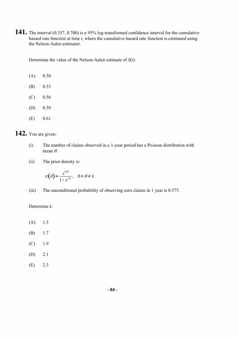
141. The interval (0.357, 0.700) is a 95% log-transformed confidence interval for the cumulativehazard rate function at time t , where the cumulative hazard rate function is estimated usingthe Nelson-Aalen estimator.
Determine the value of the Nelson-Aalen estimate of S (t ).
(A) 0.50
(B) 0.53
(C) 0.56
(D) 0.59
(E) 0.61
142. You are given:
(i) The number of claims observed in a 1-year period has a Poisson distribution withmean θ .
(ii) The prior density is:
, 01 k
e
k e
θ
π θ θ
< <
(iii) The unconditional probability of observing zero claims in 1 year is 0.575.
Determine k .
(A) 1.5
(B) 1.7
(C) 1.9
(D) 2.1
(E) 2.3
8/13/2019 Edu Exam c Sample Quest
http://slidepdf.com/reader/full/edu-exam-c-sample-quest 85/184
- 85 -
143. The parameters of the inverse Pareto distribution
( ) /F x x x τ
θ
are to be estimated using the method of moments based on the following data:
15 45 140 250 560 1340
Estimate θ by matching k th moments with k = 1 and k = 2 .
(A) Less than 1
(B) At least 1, but less than 5
(C) At least 5, but less than 25
(D) At least 25, but less than 50
(E) At least 50
144. A sample of claim amounts is {300, 600, 1500}. By applying the deductible to this sample,the loss elimination ratio for a deductible of 100 per claim is estimated to be 0.125.
You are given the following simulations from the sample:
Simulation Claim Amounts1 600 600 15002 1500 300 15003 1500 300 6004 600 600 3005 600 300 15006 600 600 15007 1500 1500 15008 1500 300 1500
9 300 600 30010 600 600 600
Determine the bootstrap approximation to the mean square error of the estimate.
8/13/2019 Edu Exam c Sample Quest
http://slidepdf.com/reader/full/edu-exam-c-sample-quest 86/184
- 86 -
(A) 0.003
(B) 0.010
(C) 0.021
(D) 0.054
(E) 0.081
145. You are given the following commercial automobile policy experience:
Company Year 1 Year 2 Year 3
Losses Number of Automobiles
I50,000
10050,000
200??
Losses Number of Automobiles
II ??
150,000500
150,000300
Losses Number of Automobiles
III150,000
50??
150,000150
Determine the nonparametric empirical Bayes credibility factor, Z , for Company III.
(A) Less than 0.2
(B) At least 0.2, but less than 0.4
(C) At least 0.4, but less than 0.6
(D) At least 0.6, but less than 0.8
(E) At least 0.8
146. Let 1 2, , ..., n x x x and 1 2, ,..., m y y y denote independent random samples of losses from
Region 1 and Region 2, respectively. Single-parameter Pareto distributions with 1θ = , but
different values of ,α are used to model losses in these regions.
Past experience indicates that the expected value of losses in Region 2 is 1.5 times theexpected value of losses in Region 1. You intend to calculate the maximum likelihoodestimate of α for Region 1, using the data from both regions.
Which of the following equations must be solved?
8/13/2019 Edu Exam c Sample Quest
http://slidepdf.com/reader/full/edu-exam-c-sample-quest 87/184
- 87 -
(A) ln 0i
n x
α =
(B) 2
2 ln2ln 0
3 2
ii
ymn x
α
α α α
=
∑∑
(C) 2
2 ln2ln 0
3 2 2
ii
yn m x
α α α α =
∑∑
(D) 2
6 ln2ln 0
2 2
ii
yn m x
α α α α =
∑∑
(E) 2
6 ln3ln 0
3 3
ii
yn m x
α α α α
=
∑∑
147. From a population having distribution function F, you are given the following sample:
2.0, 3.3, 3.3, 4.0, 4.0, 4.7, 4.7, 4.7
Calculate the kernel density estimate of F (4), using the uniform kernel with bandwidth 1.4.
(A) 0.31
(B) 0.41
(C) 0.50
(D) 0.53
(E) 0.63
8/13/2019 Edu Exam c Sample Quest
http://slidepdf.com/reader/full/edu-exam-c-sample-quest 88/184
- 88 -
148. You are given:
(i) The number of claims has probability function:
1 m x xm
p x q q x
= , x = 0, 1, 2,…, m
(ii) The actual number of claims must be within 1% of the expected number of claimswith probability 0.95.
(iii) The expected number of claims for full credibility is 34,574.
Determine q.
(A) 0.05
(B) 0.10
(C) 0.20
(D) 0.40
(E) 0.80
149. If the proposed model is appropriate, which of the following tends to zero as the sample sizegoes to infinity?
(A) Kolmogorov-Smirnov test statistic
(B) Anderson-Darling test statistic
(C) Chi-square goodness-of-fit test statistic
(D) Schwarz Bayesian adjustment
(E) None of (A), (B), (C) or (D)
8/13/2019 Edu Exam c Sample Quest
http://slidepdf.com/reader/full/edu-exam-c-sample-quest 89/184
- 89 -
150. You are given:
(i) Losses are uniformly distributed on 0,θ with θ > 150.
(ii) The policy limit is 150.
(iii) A sample of payments is:
14, 33, 72, 94, 120, 135, 150, 150
Estimate θ by matching the average sample payment to the expected payment per loss.
(A) 192
(B) 196
(C) 200
(D) 204
(E) 208
151. You are given:
(i) A portfolio of independent risks is divided into two classes.
(ii) Each class contains the same number of risks.
(iii) For each risk in Class 1, the number of claims per year follows a Poisson distributionwith mean 5.
(iv) For each risk in Class 2, the number of claims per year follows a binomial distributionwith 8=m and 55.0=q .
(v) A randomly selected risk has three claims in Year 1, r claims in Year 2 and fourclaims in Year 3.
The Bühlmann credibility estimate for the number of claims in Year 4 for this risk is 4.6019.
Determine r .

8/13/2019 Edu Exam c Sample Quest
http://slidepdf.com/reader/full/edu-exam-c-sample-quest 90/184
- 90 -
(A) 1
(B) 2
(C) 3
(D) 4
(E) 5
152. You are given:
(i) A sample of losses is:
600 700 900
(ii) No information is available about losses of 500 or less.
(iii) Losses are assumed to follow an exponential distribution with mean θ .
Determine the maximum likelihood estimate of θ .
(A) 233
(B) 400
(C) 500
(D) 733
(E) 1233
153. DELETED
8/13/2019 Edu Exam c Sample Quest
http://slidepdf.com/reader/full/edu-exam-c-sample-quest 91/184
- 91 -
154. You are given:
(v) Claim counts follow a Poisson distribution with mean λ .
(vi) Claim sizes follow a lognormal distribution with parameters µ and σ .
(vii) Claim counts and claim sizes are independent.
(viii) The prior distribution has joint probability density function:
( ), , 2 f λ µ σ σ = , 0 1λ < < , 0 1µ < < , 0 1σ < <
Calculate Bühlmann’s k for aggregate losses.
(A) Less than 2
(B) At least 2, but less than 4
(C) At least 4, but less than 6
(D) At least 6, but less than 8
(E) At least 8
155. You are given the following data:
0.49 0.51 0.66 1.82 3.71 5.20 7.62 12.66 35.24
You use the method of percentile matching at the 40th and 80th percentiles to fit an InverseWeibull distribution to these data.
Determine the estimate of θ .
8/13/2019 Edu Exam c Sample Quest
http://slidepdf.com/reader/full/edu-exam-c-sample-quest 92/184
- 92 -
(A) Less than 1.35
(B) At least 1.35, but less than 1.45
(C) At least 1.45, but less than 1.55
(D) At least 1.55, but less than 1.65
(E) At least 1.65
156. You are given:
(i) The number of claims follows a Poisson distribution with mean λ .
(ii) Observations other than 0 and 1 have been deleted from the data.
(iii) The data contain an equal number of observations of 0 and 1.
Determine the maximum likelihood estimate of λ .
(A) 0.50
(B) 0.75
(C) 1.00
(D) 1.25
(E) 1.50
157. You are given:
(i) In a portfolio of risks, each policyholder can have at most one claim per year.
(ii) The probability of a claim for a policyholder during a year is q .
(iii) The prior density is ,07.0)(
3qq =π .8.06.0 << q
A randomly selected policyholder has one claim in Year 1 and zero claimsin Year 2.
For this policyholder, determine the posterior probability that .8.07.0 << q
8/13/2019 Edu Exam c Sample Quest
http://slidepdf.com/reader/full/edu-exam-c-sample-quest 93/184
- 93 -
(A) Less than 0.3
(B) At least 0.3, but less than 0.4
(C) At least 0.4, but less than 0.5
(D) At least 0.5, but less than 0.6
(E) At least 0.6
158. You are given:
(i) The following is a sample of 15 losses:
11, 22, 22, 22, 36, 51, 69, 69, 69, 92, 92, 120, 161, 161, 230
(ii) 1ˆ ( ) x H is the Nelson-Aalen empirical estimate of the cumulative hazard rate function.
(iii) 2ˆ ( ) H x is the maximum likelihood estimate of the cumulative hazard rate function
under the assumption that the sample is drawn from an exponential distribution.
Calculate 2 1ˆ ˆ(75) (75) H H .
(A) 0.00
(B) 0.11
(C) 0.22
(D) 0.33
(E) 0.44
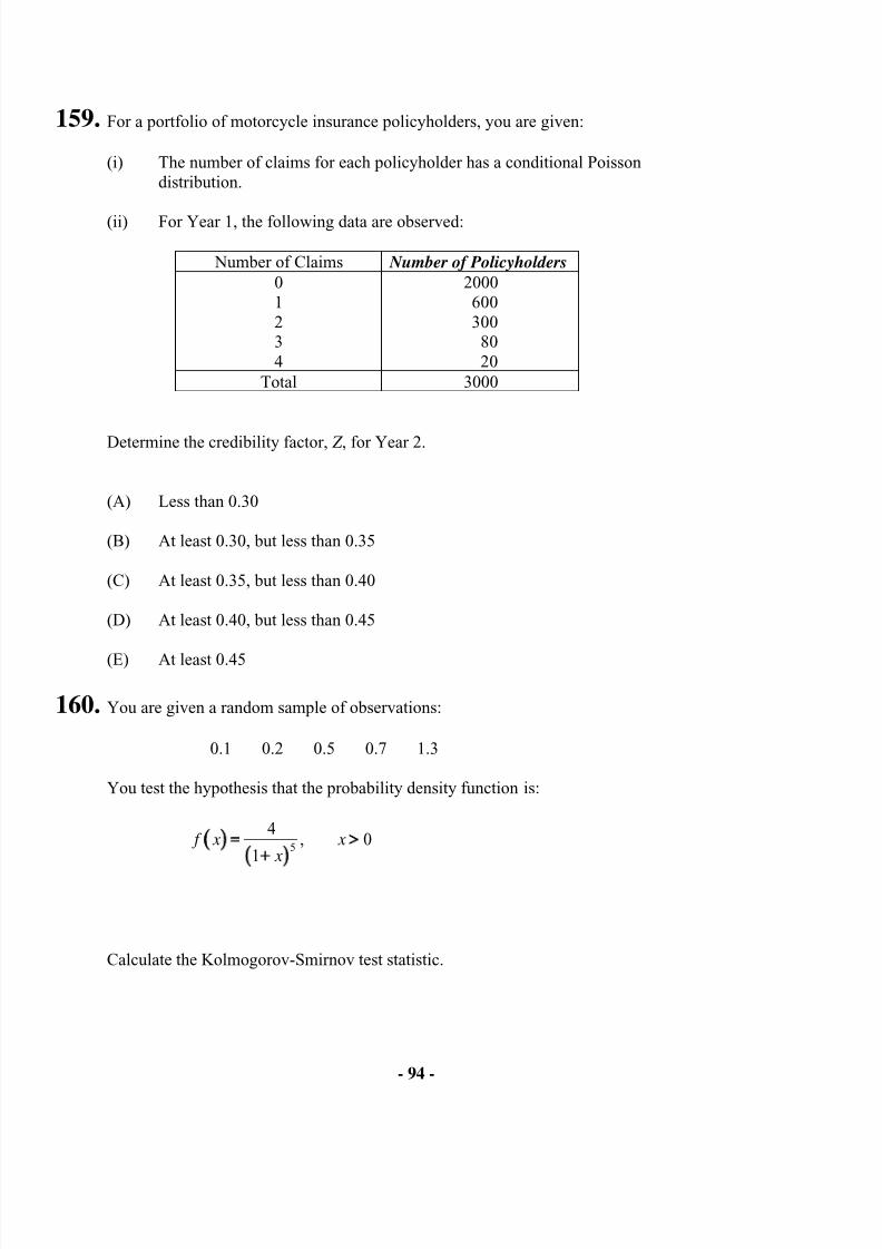
8/13/2019 Edu Exam c Sample Quest
http://slidepdf.com/reader/full/edu-exam-c-sample-quest 94/184
- 94 -
159. For a portfolio of motorcycle insurance policyholders, you are given:
(i) The number of claims for each policyholder has a conditional Poissondistribution.
(ii) For Year 1, the following data are observed:
Number of Claims Number of Policyholders
0 20001 6002 3003 804 20
Total 3000
Determine the credibility factor, Z , for Year 2.
(A) Less than 0.30
(B) At least 0.30, but less than 0.35
(C) At least 0.35, but less than 0.40
(D) At least 0.40, but less than 0.45
(E) At least 0.45
160. You are given a random sample of observations:
0.1 0.2 0.5 0.7 1.3
You test the hypothesis that the probability density function is:
5
4, 0
1 f x x
x= >
Calculate the Kolmogorov-Smirnov test statistic.
8/13/2019 Edu Exam c Sample Quest
http://slidepdf.com/reader/full/edu-exam-c-sample-quest 95/184
- 95 -
(A) Less than 0.05
(B) At least 0.05, but less than 0.15
(C) At least 0.15, but less than 0.25
(D) At least 0.25, but less than 0.35
(E) At least 0.35
161. Which of the following statements is true?
(A) A uniformly minimum variance unbiased estimator is an estimator such that no otherestimator has a smaller variance.
(B) An estimator is consistent whenever the variance of the estimator approaches zero as
the sample size increases to infinity.
(C) A consistent estimator is also unbiased.
(D) For an unbiased estimator, the mean squared error is always equal to the variance.
(E) One computational advantage of using mean squared error is that it is not a functionof the true value of the parameter.
162. A loss, X , follows a 2-parameter Pareto distribution with 2α = and unspecified parameter
θ . You are given:
5E 100 100 E 50 50
3 X X X X − > = − >
Calculate E 150 150 X X − > .
(A) 150
(B) 175
(C) 200
(D) 225
(E) 250
8/13/2019 Edu Exam c Sample Quest
http://slidepdf.com/reader/full/edu-exam-c-sample-quest 96/184
- 96 -
163. The scores on the final exam in Ms. B’s Latin class have a normal distribution with mean θ and standard deviation equal to 8. θ is a random variable with a normal distribution withmean equal to 75 and standard deviation equal to 6.
Each year, Ms. B chooses a student at random and pays the student 1 times the student’s
score. However, if the student fails the exam (score 65≤ ), then there is no payment.
Calculate the conditional probability that the payment is less than 90, given that there is a payment.
(A) 0.77
(B) 0.85
(C) 0.88
(D) 0.92
(E) 1.00
164. For a collective risk model the number of losses, N, has a Poisson distribution with 20λ = .The common distribution of the individual losses has the following characteristics:
(i) [ ]E 70 X =
(ii) [ ]E 30 25 X ∧ =
(iii) ( )Pr 30 0.75 X > =
(iv) 2E 30 9000 X X > =
An insurance covers aggregate losses subject to an ordinary deductible of 30 per loss.
Calculate the variance of the aggregate payments of the insurance.
(A) 54,000
(B) 67,500
(C) 81,000
(D) 94,500
(E) 108,000
8/13/2019 Edu Exam c Sample Quest
http://slidepdf.com/reader/full/edu-exam-c-sample-quest 97/184
- 97 -
165. For a collective risk model:
(i) The number of losses has a Poisson distribution with 2λ = .
(ii) The common distribution of the individual losses is:
x ( ) x f x
1 0.6
2 0.4
An insurance covers aggregate losses subject to a deductible of 3.
Calculate the expected aggregate payments of the insurance.
(A) 0.74
(B) 0.79
(C) 0.84
(D) 0.89
(E) 0.94
166. A discrete probability distribution has the following properties:
(i) 1
11k k p c p
k −
= +
for k = 1, 2,…
(ii) 0 0.5 p =
Calculate c.
(A) 0.06
(B) 0.13
(C) 0.29
(D) 0.35
(E) 0.40
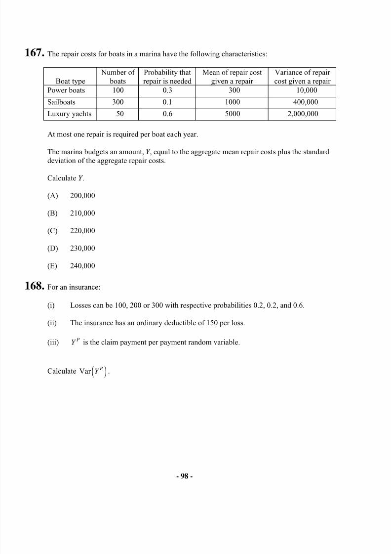
8/13/2019 Edu Exam c Sample Quest
http://slidepdf.com/reader/full/edu-exam-c-sample-quest 98/184
- 98 -
167. The repair costs for boats in a marina have the following characteristics:
Boat type Number of
boatsProbability thatrepair is needed
Mean of repair costgiven a repair
Variance of repaircost given a repair
Power boats 100 0.3 300 10,000
Sailboats 300 0.1 1000 400,000
Luxury yachts 50 0.6 5000 2,000,000
At most one repair is required per boat each year.
The marina budgets an amount, Y , equal to the aggregate mean repair costs plus the standarddeviation of the aggregate repair costs.
Calculate Y .
(A) 200,000
(B) 210,000
(C) 220,000
(D) 230,000
(E) 240,000
168.For an insurance:
(i) Losses can be 100, 200 or 300 with respective probabilities 0.2, 0.2, and 0.6.
(ii) The insurance has an ordinary deductible of 150 per loss.
(iii) PY is the claim payment per payment random variable.
Calculate ( )Var PY .
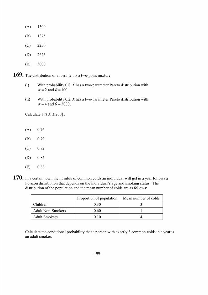
8/13/2019 Edu Exam c Sample Quest
http://slidepdf.com/reader/full/edu-exam-c-sample-quest 99/184
8/13/2019 Edu Exam c Sample Quest
http://slidepdf.com/reader/full/edu-exam-c-sample-quest 100/184
- 100 -
(A) 0.12
(B) 0.16
(C) 0.20
(D) 0.24
(E) 0.28
171. For aggregate losses, S :
(i) The number of losses has a negative binomial distribution with mean 3 andvariance 3.6.
(ii) The common distribution of the independent individual loss amounts is uniform from
0 to 20.
Calculate the 95th percentile of the distribution of S as approximated by the normaldistribution.
(A) 61
(B) 63
(C) 65
(D) 67
(E) 69
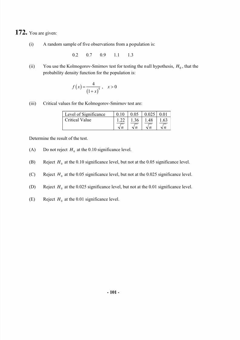
8/13/2019 Edu Exam c Sample Quest
http://slidepdf.com/reader/full/edu-exam-c-sample-quest 101/184
- 101 -
172. You are given:
(i) A random sample of five observations from a population is:
0.2 0.7 0.9 1.1 1.3
(ii) You use the Kolmogorov-Smirnov test for testing the null hypothesis, 0 H , that the
probability density function for the population is:
( )( )
5
4, 0
1 f x x
x= >
+
(iii) Critical values for the Kolmogorov-Smirnov test are:
Level of Significance 0.10 0.05 0.025 0.01
Critical Valuen
22.1 n
36.1 n
48.1 n
63.1
Determine the result of the test.
(A) Do not reject 0 H at the 0.10 significance level.
(B) Reject 0 H at the 0.10 significance level, but not at the 0.05 significance level.
(C) Reject 0 H at the 0.05 significance level, but not at the 0.025 significance level.
(D) Reject 0 H at the 0.025 significance level, but not at the 0.01 significance level.
(E) Reject 0 H at the 0.01 significance level.
8/13/2019 Edu Exam c Sample Quest
http://slidepdf.com/reader/full/edu-exam-c-sample-quest 102/184
- 102 -
173. You are given:
(iv) The number of claims follows a negative binomial distribution with parameters r and3= β .
(v) Claim severity has the following distribution:
Claim Size Probability
1 0.4
10 0.4
100 0.2
(iii) The number of claims is independent of the severity of claims.
Determine the expected number of claims needed for aggregate losses to be within 10% ofexpected aggregate losses with 95% probability.
(A) Less than 1200
(B) At least 1200, but less than 1600
(C) At least 1600, but less than 2000
(D) At least 2000, but less than 2400(E) At least 2400
174. You are given:
(vi) A mortality study covers n lives.
(vii) None were censored and no two deaths occurred at the same time.
(viii) =k t time of the thk death
(ix) A Nelson-Aalen estimate of the cumulative hazard rate function is380
39)(ˆ
2 =t H .
Determine the Kaplan-Meier product-limit estimate of the survival function at time 9t .
8/13/2019 Edu Exam c Sample Quest
http://slidepdf.com/reader/full/edu-exam-c-sample-quest 103/184
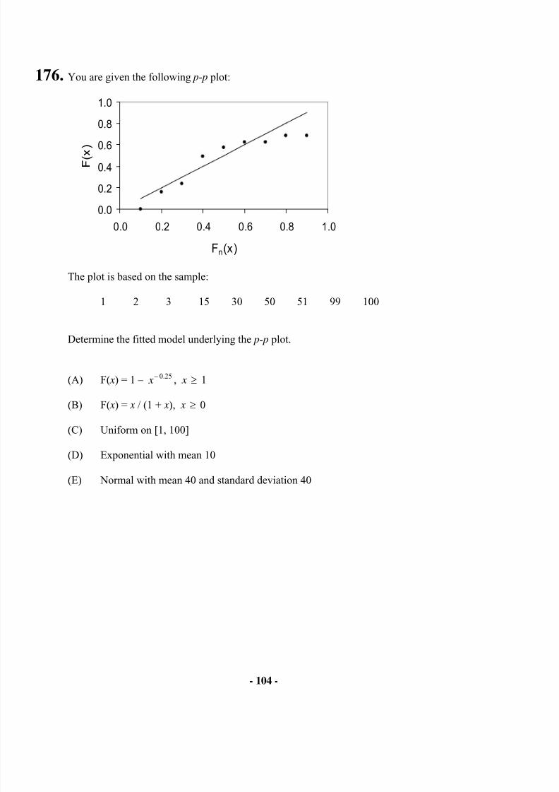
8/13/2019 Edu Exam c Sample Quest
http://slidepdf.com/reader/full/edu-exam-c-sample-quest 104/184
- 104 -
176. You are given the following p- p plot:
0.0
0.2
0.4
0.6
0.8
1.0
0.0 0.2 0.4 0.6 0.8 1.0
Fn(x)
F ( x )
The plot is based on the sample:
1 2 3 15 30 50 51 99 100
Determine the fitted model underlying the p- p plot.
(A) F( x) = 1 – 0.25 x− , x ≥ 1
(B) F( x) = x / (1 + x), x ≥ 0
(C) Uniform on [1, 100]
(D) Exponential with mean 10
(E) Normal with mean 40 and standard deviation 40
8/13/2019 Edu Exam c Sample Quest
http://slidepdf.com/reader/full/edu-exam-c-sample-quest 105/184
- 105 -
177. You are given:
(i) Claims are conditionally independent and identically Poisson distributed withmean Θ .
(ii) The prior distribution function of Θ is:
2.61
( ) 11
F θ θ
= − +
, 0θ >
Five claims are observed.
Determine the Bühlmann credibility factor.
(A) Less than 0.6
(B) At least 0.6, but less than 0.7
(C) At least 0.7, but less than 0.8
(D) At least 0.8, but less than 0.9
(E) At least 0.9
178. DELETED
179-180. Use the following information for questions 179 and 180.
The time to an accident follows an exponential distribution. A random sample of size twohas a mean time of 6.
Let Y denote the mean of a new sample of size two.
179. Determine the maximum likelihood estimate of ( )Pr 10Y > .
(A) 0.04
(B) 0.07
(C) 0.11
(D) 0.15
(E) 0.19
8/13/2019 Edu Exam c Sample Quest
http://slidepdf.com/reader/full/edu-exam-c-sample-quest 106/184
- 106 -
180. Use the delta method to approximate the variance of the maximum likelihood estimator of
(10)Y F .
(A) 0.08
(B) 0.12
(C) 0.16
(D) 0.19
(E) 0.22
181. You are given:
(i) The number of claims in a year for a selected risk follows a Poisson distribution withmean λ .
(ii) The severity of claims for the selected risk follows an exponential distribution withmean .θ
(iii) The number of claims is independent of the severity of claims.
(iv) The prior distribution of λ is exponential with mean 1.
(v) The prior distribution of θ is Poisson with mean 1.
(vi) A priori, λ and θ are independent.
Using Bühlmann’s credibility for aggregate losses, determine k .
(A) 1
(B) 4/3
(C) 2
(D) 3
(E) 4
8/13/2019 Edu Exam c Sample Quest
http://slidepdf.com/reader/full/edu-exam-c-sample-quest 107/184
- 107 -
182. A company insures 100 people age 65. The annual probability of death for each person is0.03. The deaths are independent.
Use the inversion method to simulate the number of deaths in a year. Do this three times
using:1
2
3
0.20
0.03
0.09
u
u
u
=
=
=
Calculate the average of the simulated values.
(A) 13
(B) 1
(C) 53
(D) 73
(E) 3
183. You are given claim count data for which the sample mean is roughly equal to the samplevariance. Thus you would like to use a claim count model that has its mean equal to itsvariance. An obvious choice is the Poisson distribution.
Determine which of the following models may also be appropriate.
(A) A mixture of two binomial distributions with different means
(B) A mixture of two Poisson distributions with different means
(C) A mixture of two negative binomial distributions with different means
(D) None of (A), (B) or (C)
(E) All of (A), (B) and (C)
8/13/2019 Edu Exam c Sample Quest
http://slidepdf.com/reader/full/edu-exam-c-sample-quest 108/184
8/13/2019 Edu Exam c Sample Quest
http://slidepdf.com/reader/full/edu-exam-c-sample-quest 109/184
- 109 -
186. For the random variable X , you are given:
(i) [ ]E X θ = , 0θ >
(ii) ( )2
Var 25
X θ =
(iii) ˆ ,1
k X
k θ =
+ 0k >
(iv) ( ) ( ) 2
ˆ ˆMSE 2 biasθ θ
θ θ =
Determine k .
(A) 0.2
(B) 0.5
(C) 2
(D) 5
(E) 25
187.You are given:
(i) The annual number of claims on a given policy has a geometric distribution with parameter β .
(ii) The prior distribution of β has the Pareto density function
( 1)( ) , 0
( 1) α
α π β β
β +
= < < ∞+
,
where α is a known constant greater than 2.
A randomly selected policy had x claims in Year 1.
Determine the Bühlmann credibility estimate of the number of claims for the selected policyin Year 2.
8/13/2019 Edu Exam c Sample Quest
http://slidepdf.com/reader/full/edu-exam-c-sample-quest 110/184
- 110 -
(A)1
1α −
(B)( 1) 1
( 1)
xα
α α α
−+
−
(C) x
(D)1 x
α
+
(E)1
1
x
α
+
−
188. DELETED
189. Which of the following statements is true?
(A) For a null hypothesis that the population follows a particular distribution, usingsample data to estimate the parameters of the distribution tends to decrease the probability of a Type II error.
(B) The Kolmogorov-Smirnov test can be used on individual or grouped data.
(C) The Anderson-Darling test tends to place more emphasis on a good fit in the middle
rather than in the tails of the distribution.
(D) For a given number of cells, the critical value for the chi-square goodness-of-fit test becomes larger with increased sample size.
(E) None of (A), (B), (C) or (D) is true.
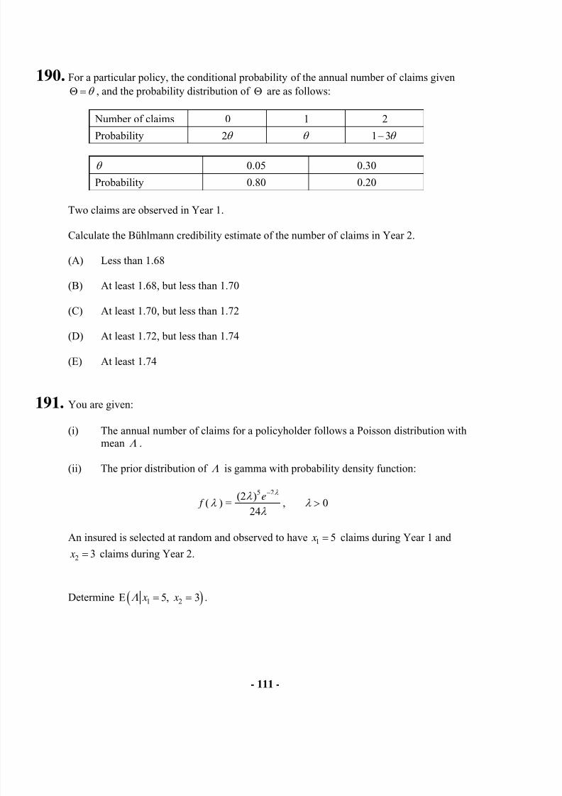
8/13/2019 Edu Exam c Sample Quest
http://slidepdf.com/reader/full/edu-exam-c-sample-quest 111/184
- 111 -
190. For a particular policy, the conditional probability of the annual number of claims givenθ Θ = , and the probability distribution of Θ are as follows:
Number of claims 0 1 2
Probability 2θ θ 1 3θ −
θ 0.05 0.30
Probability 0.80 0.20
Two claims are observed in Year 1.
Calculate the Bühlmann credibility estimate of the number of claims in Year 2.
(A) Less than 1.68
(B) At least 1.68, but less than 1.70
(C) At least 1.70, but less than 1.72
(D) At least 1.72, but less than 1.74
(E) At least 1.74
191. You are given:
(i) The annual number of claims for a policyholder follows a Poisson distribution withmean Λ .
(ii) The prior distribution of Λ is gamma with probability density function:
f ( λ ) =5 2(2 )
24
e λ λ
λ
−
, 0λ >
An insured is selected at random and observed to have 1 5 x = claims during Year 1 and
2 3 x = claims during Year 2.
Determine ( )1 2E 5, 3 x xΛ = = .
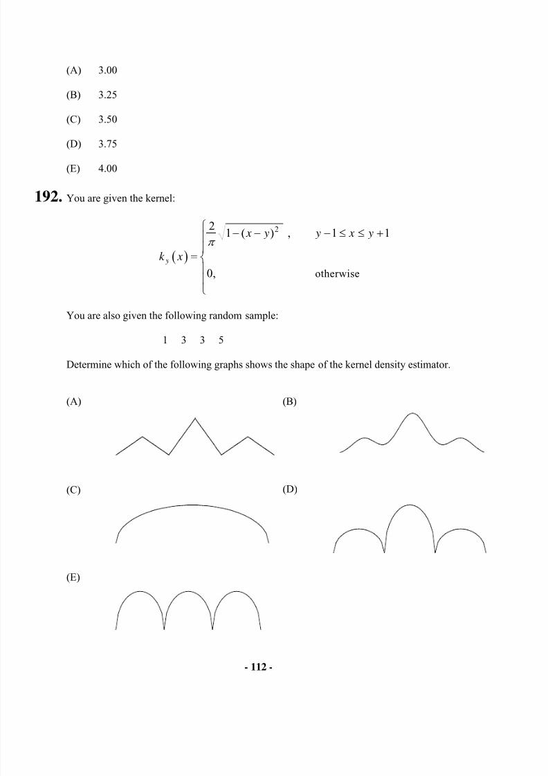
8/13/2019 Edu Exam c Sample Quest
http://slidepdf.com/reader/full/edu-exam-c-sample-quest 112/184
- 112 -
(A) 3.00
(B) 3.25
(C) 3.50
(D) 3.75
(E) 4.00
192. You are given the kernel:
( )
2
otherwise
21 ( ) , 1 1
0,
y
x y y x y
k x
π
− − − ≤ ≤ +
=
You are also given the following random sample:
1 3 3 5
Determine which of the following graphs shows the shape of the kernel density estimator.
(A)
(C)
(E)
(B)
(D)
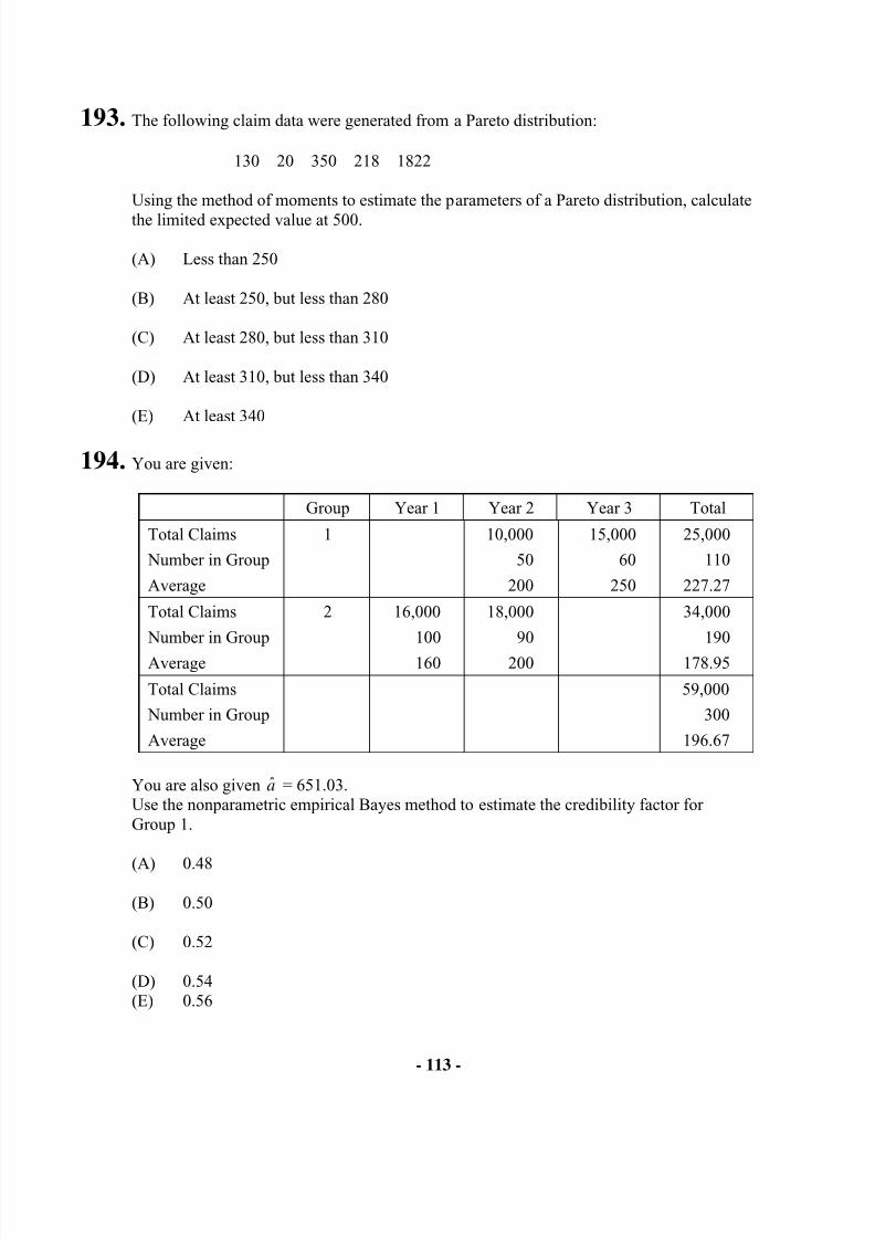
8/13/2019 Edu Exam c Sample Quest
http://slidepdf.com/reader/full/edu-exam-c-sample-quest 113/184
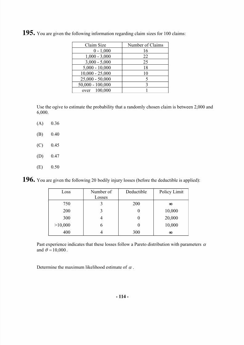
8/13/2019 Edu Exam c Sample Quest
http://slidepdf.com/reader/full/edu-exam-c-sample-quest 114/184
- 114 -
195. You are given the following information regarding claim sizes for 100 claims:
Claim Size Number of Claims0 - 1,000 16
1,000 - 3,000 22
3,000 - 5,000 255,000 - 10,000 18
10,000 - 25,000 1025,000 - 50,000 5
50,000 - 100,000 3over 100,000 1
Use the ogive to estimate the probability that a randomly chosen claim is between 2,000 and6,000.
(A) 0.36
(B) 0.40
(C) 0.45
(D) 0.47
(E) 0.50
196. You are given the following 20 bodily injury losses (before the deductible is applied):
Loss Number ofLosses
Deductible Policy Limit
750 3 200 ∞
200 3 0 10,000
300 4 0 20,000
>10,000 6 0 10,000
400 4 300 ∞
Past experience indicates that these losses follow a Pareto distribution with parameters α and 10,000θ = .
Determine the maximum likelihood estimate of α .
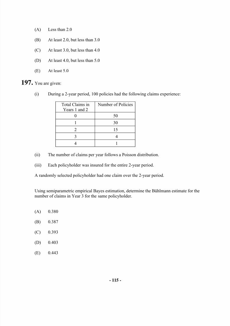
8/13/2019 Edu Exam c Sample Quest
http://slidepdf.com/reader/full/edu-exam-c-sample-quest 115/184
- 115 -
(A) Less than 2.0
(B) At least 2.0, but less than 3.0
(C) At least 3.0, but less than 4.0
(D) At least 4.0, but less than 5.0
(E) At least 5.0
197. You are given:
(i) During a 2-year period, 100 policies had the following claims experience:
Total Claims inYears 1 and 2
Number of Policies
0 50
1 30
2 15
3 4
4 1
(ii) The number of claims per year follows a Poisson distribution.
(iii) Each policyholder was insured for the entire 2-year period.
A randomly selected policyholder had one claim over the 2-year period.
Using semiparametric empirical Bayes estimation, determine the Bühlmann estimate for thenumber of claims in Year 3 for the same policyholder.
(A) 0.380
(B) 0.387
(C) 0.393
(D) 0.403
(E) 0.443
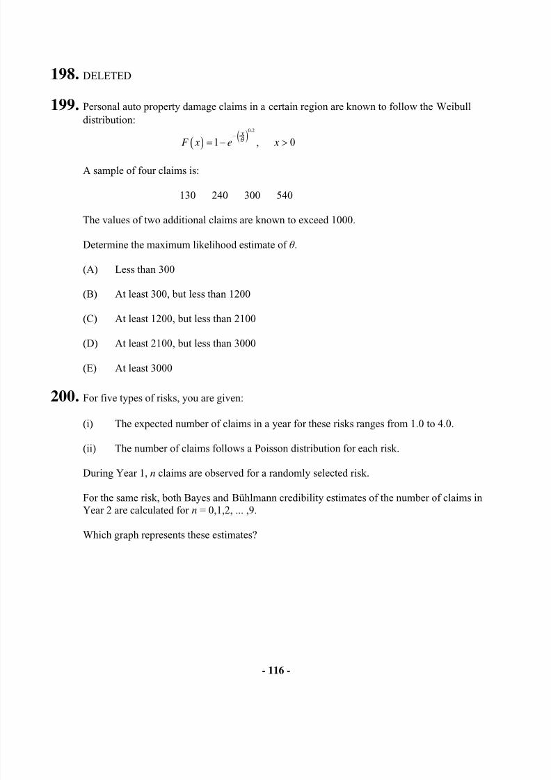
8/13/2019 Edu Exam c Sample Quest
http://slidepdf.com/reader/full/edu-exam-c-sample-quest 116/184
- 116 -
198. DELETED
199. Personal auto property damage claims in a certain region are known to follow the Weibulldistribution:
( ) ( )0.2
1 , 0 xF x e xθ −= − >
A sample of four claims is:
130 240 300 540
The values of two additional claims are known to exceed 1000.
Determine the maximum likelihood estimate of θ .
(A) Less than 300
(B) At least 300, but less than 1200
(C) At least 1200, but less than 2100
(D) At least 2100, but less than 3000
(E) At least 3000
200. For five types of risks, you are given:
(i) The expected number of claims in a year for these risks ranges from 1.0 to 4.0.
(ii) The number of claims follows a Poisson distribution for each risk.
During Year 1, n claims are observed for a randomly selected risk.
For the same risk, both Bayes and Bühlmann credibility estimates of the number of claims inYear 2 are calculated for n = 0,1,2, ... ,9.
Which graph represents these estimates?
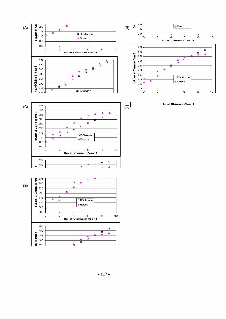
8/13/2019 Edu Exam c Sample Quest
http://slidepdf.com/reader/full/edu-exam-c-sample-quest 117/184
- 117 -
(A) (B)
(C) (D)
(E)
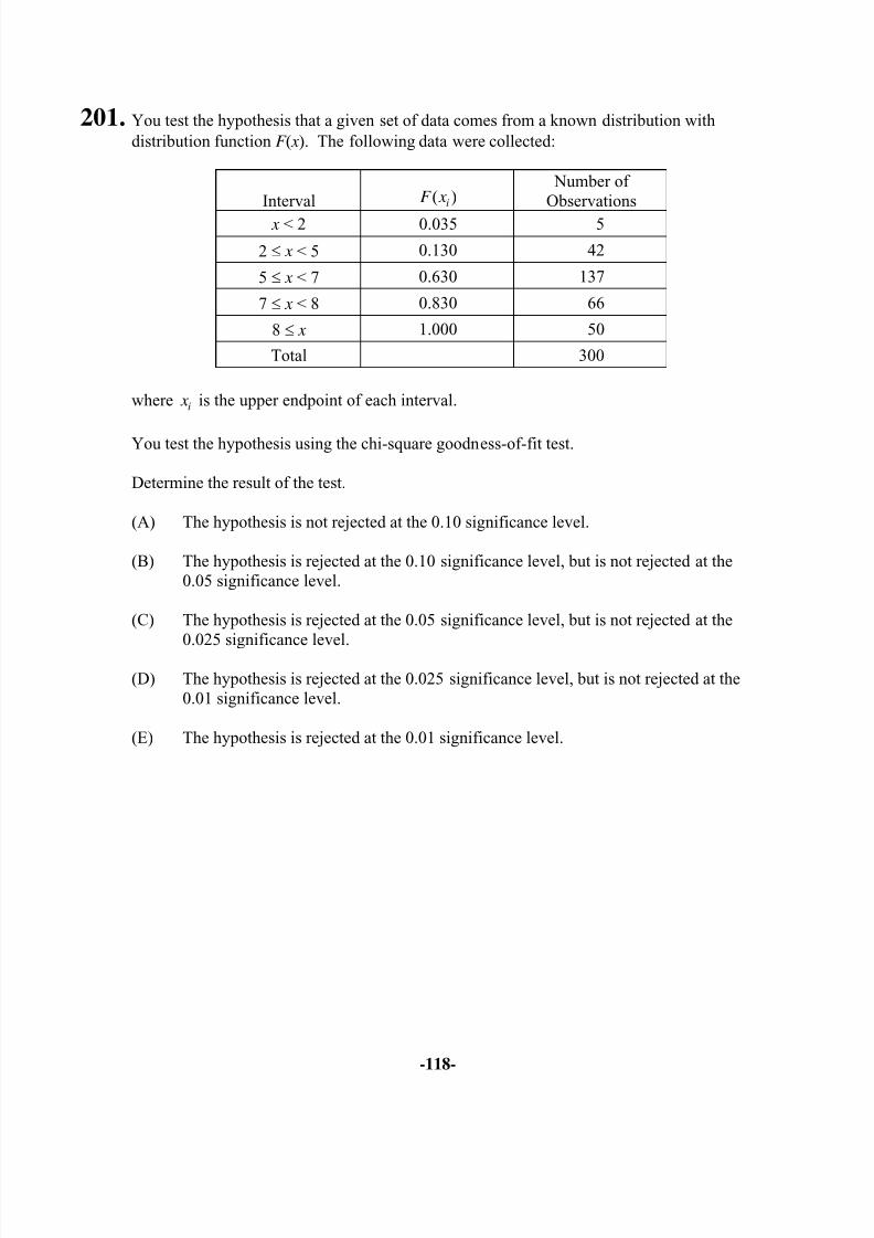
8/13/2019 Edu Exam c Sample Quest
http://slidepdf.com/reader/full/edu-exam-c-sample-quest 118/184
-118-
201. You test the hypothesis that a given set of data comes from a known distribution withdistribution function F ( x). The following data were collected:
Interval ( )iF x Number ofObservations
x < 2 0.035 5
2 ≤ x < 5 0.130 42
5 ≤ x < 7 0.630 137
7 ≤ x < 8 0.830 66
8 ≤ x 1.000 50
Total 300
where i x is the upper endpoint of each interval.
You test the hypothesis using the chi-square goodness-of-fit test.
Determine the result of the test.
(A) The hypothesis is not rejected at the 0.10 significance level.
(B) The hypothesis is rejected at the 0.10 significance level, but is not rejected at the0.05 significance level.
(C) The hypothesis is rejected at the 0.05 significance level, but is not rejected at the0.025 significance level.
(D) The hypothesis is rejected at the 0.025 significance level, but is not rejected at the0.01 significance level.
(E) The hypothesis is rejected at the 0.01 significance level.
8/13/2019 Edu Exam c Sample Quest
http://slidepdf.com/reader/full/edu-exam-c-sample-quest 119/184
-119-
202. Unlimited claim severities for a warranty product follow the lognormal distribution with parameters 5.6µ = and 0.75σ = .
You use simulation to generate severities.
The following are six uniform (0, 1) random numbers:
0.6179 0.4602 0.9452 0.0808 0.7881 0.4207
Using these numbers and the inversion method, calculate the average payment per claimfor a contract with a policy limit of 400.
(A) Less than 300
(B) At least 300, but less than 320
(C) At least 320, but less than 340
(D) At least 340, but less than 360
(E) At least 360
203. You are given:
(i) The annual number of claims on a given policy has the geometric distributionwith parameter β .
(ii) One-third of the policies have β = 2, and the remaining two-thirds have β = 5.
A randomly selected policy had two claims in Year 1.
Calculate the Bayesian expected number of claims for the selected policy in Year 2.
(A) 3.4
(B) 3.6
(C) 3.8
(D) 4.0
(E) 4.2
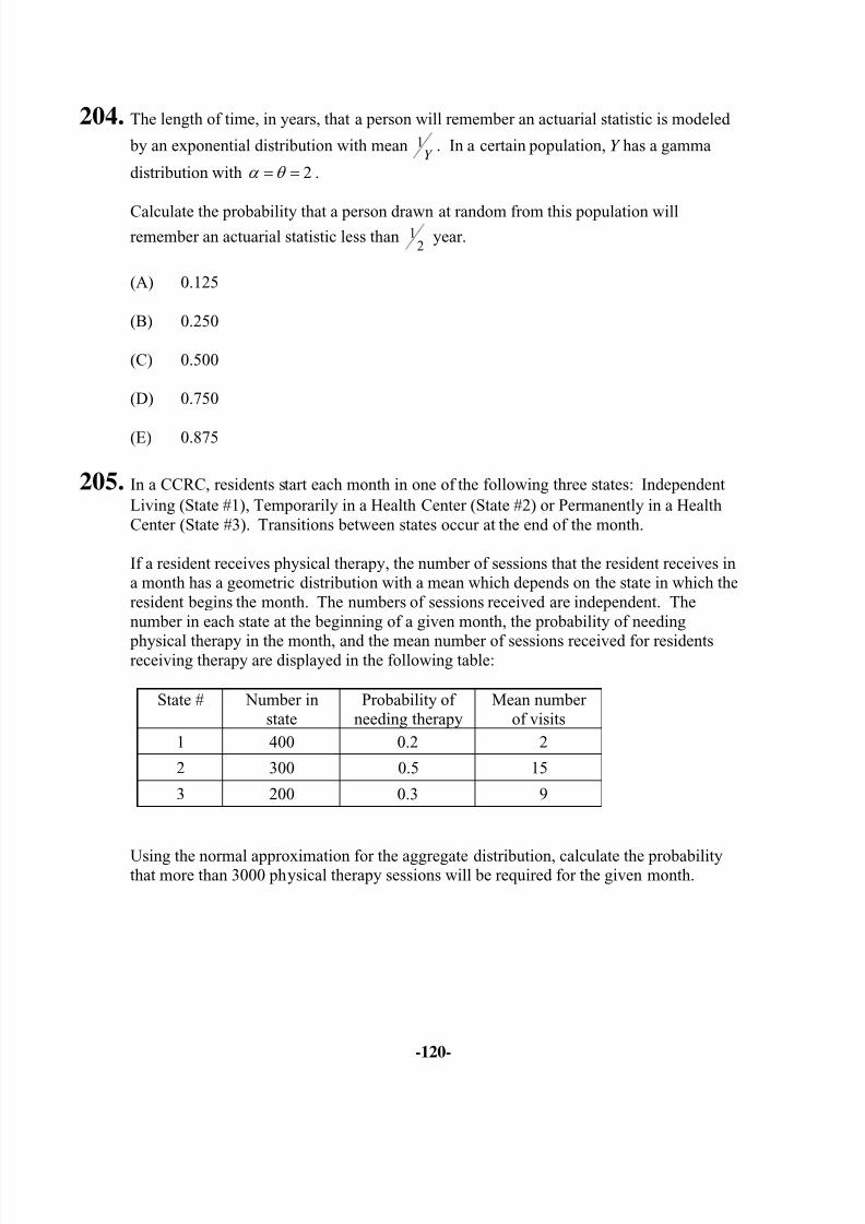
8/13/2019 Edu Exam c Sample Quest
http://slidepdf.com/reader/full/edu-exam-c-sample-quest 120/184
8/13/2019 Edu Exam c Sample Quest
http://slidepdf.com/reader/full/edu-exam-c-sample-quest 121/184
8/13/2019 Edu Exam c Sample Quest
http://slidepdf.com/reader/full/edu-exam-c-sample-quest 122/184
-122-
207. For an insurance:
(i) Losses have density function
( )0.02 0 10
0 elsewhere X
x x
f x
< <
=
(ii) The insurance has an ordinary deductible of 4 per loss.
(iii) PY is the claim payment per payment random variable.
Calculate E PY .
(A) 2.9
(B) 3.0
(C) 3.2
(D) 3.3
(E) 3.4
208. An actuary has created a compound claims frequency model with the following properties:
(i) The primary distribution is the negative binomial with probability generatingfunction
( ) ( ) 2
1 3 1P z z −
= − − .
(ii) The secondary distribution is the Poisson with probability generating function
( ) ( )1 zP z e
λ −= .
(iii) The probability of no claims equals 0.067.
Calculate λ .
8/13/2019 Edu Exam c Sample Quest
http://slidepdf.com/reader/full/edu-exam-c-sample-quest 123/184
-123-
(A) 0.1
(B) 0.4
(C) 1.6
(D) 2.7
(E) 3.1
209. In 2005 a risk has a two-parameter Pareto distribution with 2α = and 3000θ = . In 2006losses inflate by 20%.
An insurance on the risk has a deductible of 600 in each year. iP , the premium in year i,
equals 1.2 times the expected claims.
The risk is reinsured with a deductible that stays the same in each year. i R , the
reinsurance premium in year i, equals 1.1 times the expected reinsured claims.
2005
20050.55
RP =
Calculate 2006
2006
RP .
(A) 0.46
(B) 0.52
(C) 0.55
(D) 0.58
(E) 0.66
8/13/2019 Edu Exam c Sample Quest
http://slidepdf.com/reader/full/edu-exam-c-sample-quest 124/184
-124-
210. Each life within a group medical expense policy has loss amounts which follow acompound Poisson process with 0.16λ = . Given a loss, the probability that it is forDisease 1 is 1
16 .
Loss amount distributions have the following parameters:
Mean per lossStandard
Deviation per lossDisease 1 5 50
Other diseases 10 20
Premiums for a group of 100 independent lives are set at a level such that the probability(using the normal approximation to the distribution for aggregate losses) that aggregatelosses for the group will exceed aggregate premiums for the group is 0.24.
A vaccine which will eliminate Disease 1 and costs 0.15 per person has been discovered.
Define:A = the aggregate premium assuming that no one obtains the vaccine, andB = the aggregate premium assuming that everyone obtains the vaccine and the cost of
the vaccine is a covered loss.
Calculate A/B.
(A) 0.94
(B) 0.97
(C) 1.00
(D) 1.03
(E) 1.06
8/13/2019 Edu Exam c Sample Quest
http://slidepdf.com/reader/full/edu-exam-c-sample-quest 125/184
-125-
211. An actuary for a medical device manufacturer initially models the failure time for a particular device with an exponential distribution with mean 4 years.
This distribution is replaced with a spliced model whose density function:
(i) is uniform over [0, 3]
(ii) is proportional to the initial modeled density function after 3 years
(iii) is continuous
Calculate the probability of failure in the first 3 years under the revised distribution.
(A) 0.43
(B) 0.45
(C) 0.47
(D) 0.49
(E) 0.51
212. For an insurance:
(i) The number of losses per year has a Poisson distribution with 10λ = .
(ii) Loss amounts are uniformly distributed on (0, 10).
(iii) Loss amounts and the number of losses are mutually independent.
(iv) There is an ordinary deductible of 4 per loss.
Calculate the variance of aggregate payments in a year.
(A) 36
(B) 48
(C) 72
(D) 96
(E) 120
8/13/2019 Edu Exam c Sample Quest
http://slidepdf.com/reader/full/edu-exam-c-sample-quest 126/184
-126-
213. For an insurance portfolio:
(i) The number of claims has the probability distribution
n n p
0 0.1
1 0.4
2 0.3
3 0.2
(ii) Each claim amount has a Poisson distribution with mean 3; and
(iii) The number of claims and claim amounts are mutually independent.
Calculate the variance of aggregate claims.
(A) 4.8
(B) 6.4
(C) 8.0
(D) 10.2
(E) 12.4
214. A portfolio of policies has produced the following claims:
100 100 100 200 300 300 300 400 500 600
Determine the empirical estimate of H (300).
(A) Less than 0.50
(B) At least 0.50, but less than 0.75
(C) At least 0.75, but less than 1.00
(D) At least 1.00, but less than 1.25
(E) At least 1.25
8/13/2019 Edu Exam c Sample Quest
http://slidepdf.com/reader/full/edu-exam-c-sample-quest 127/184
-127-
215. You are given:
(i) The conditional distribution of the number of claims per policyholder is Poissonwith mean λ .
(ii) The variable λ has a gamma distribution with parameters α and θ .
(iii) For policyholders with 1 claim in Year 1, the credibility estimate for the numberof claims in Year 2 is 0.15.
(iv) For policyholders with an average of 2 claims per year in Year 1 and Year 2, thecredibility estimate for the number of claims in Year 3 is 0.20.
Determine θ .
(A) Less than 0.02
(B) At least 0.02, but less than 0.03
(C) At least 0.03, but less than 0.04
(D) At least 0.04, but less than 0.05
(E) At least 0.05
216. A random sample of claims has been drawn from a Burr distribution with known parameterα = 1 and unknown parameters θ and γ . You are given:
(i) 75% of the claim amounts in the sample exceed 100.
(ii) 25% of the claim amounts in the sample exceed 500.
Estimate θ by percentile matching.
(A) Less than 190
(B) At least 190, but less than 200
(C) At least 200, but less than 210
(D) At least 210, but less than 220
8/13/2019 Edu Exam c Sample Quest
http://slidepdf.com/reader/full/edu-exam-c-sample-quest 128/184
-128-
(E) At least 220
217. For a portfolio of policies, you are given:
(i) There is no deductible and the policy limit varies by policy.
(ii) A sample of ten claims is:
350 350 500 500 500+ 1000 1000+ 1000+ 1200 1500
where the symbol + indicates that the loss exceeds the policy limit.
(iii) ^
1(1250)S is the product-limit estimate of S (1250).
(iv) ^
2(1250)S is the maximum likelihood estimate of S (1250) under the assumption
that the losses follow an exponential distribution.
Determine the absolute difference between^
1(1250)S and^
2(1250)S .
(A) 0.00
(B) 0.03
(C) 0.05
(D) 0.07
(E) 0.09
218. The random variable X has survival function:
( )( )
4
22 2 X S x
x
θ
θ =
+
Two values of X are observed to be 2 and 4. One other value exceeds 4.
Calculate the maximum likelihood estimate of θ .
8/13/2019 Edu Exam c Sample Quest
http://slidepdf.com/reader/full/edu-exam-c-sample-quest 129/184
-129-
(A) Less than 4.0
(B) At least 4.0, but less than 4.5
(C) At least 4.5, but less than 5.0
(D) At least 5.0, but less than 5.5
(E) At least 5.5
219. For a portfolio of policies, you are given:
(i) The annual claim amount on a policy has probability density function:
2
2( | ) , 0
x f x xθ θ
θ = < <
(ii) The prior distribution of θ has density function:
3( ) 4 , 0 1π θ θ θ = < <
(iii) A randomly selected policy had claim amount 0.1 in Year 1.
Determine the Bühlmann credibility estimate of the claim amount for the selected policyin Year 2.
(A) 0.43
(B) 0.45
(C) 0.50
(D) 0.53
(E) 0.56
8/13/2019 Edu Exam c Sample Quest
http://slidepdf.com/reader/full/edu-exam-c-sample-quest 130/184
-130-
220. Total losses for a group of insured motorcyclists are simulated using the aggregate lossmodel and the inversion method.
The number of claims has a Poisson distribution with 4λ = . The amount of each claimhas an exponential distribution with mean 1000.
The number of claims is simulated using 0.13u = . The claim amounts are simulatedusing 1 0.05u = , 2 0.95u = and 3 0.10u = in that order, as needed.
Determine the total losses.
(A) 0
(B) 51
(C) 2996
(D) 3047
(E) 3152
221. You are given:
(i) The sample:
1 2 3 3 3 3 3 3 3 3
(ii) )(ˆ1 xF is the kernel density estimator of the distribution function using a uniform
kernel with bandwidth 1.
(iii) )(ˆ2 xF is the kernel density estimator of the distribution function using a
triangular kernel with bandwidth 1.
Determine which of the following intervals has )(ˆ1 xF = )(ˆ
2 xF for all x in the interval.
(A) 10 << x
(B) 21 << x
(C) 32 << x
(D) 43 << x
(E) None of (A), (B), (C) or (D)
8/13/2019 Edu Exam c Sample Quest
http://slidepdf.com/reader/full/edu-exam-c-sample-quest 131/184
-131-
222. 1000 workers insured under a workers compensation policy were observed for one year.The number of work days missed is given below:
Number of Days of WorkMissed
Number of Workers
0 8181 153
2 25
3 or more 4
Total 1000
Total Number of Days Missed 230
The chi-square goodness-of-fit test is used to test the hypothesis that the number of workdays missed follows a Poisson distribution where:
(i) The Poisson parameter is estimated by the average number of work days missed.
(ii) Any interval in which the expected number is less than one is combined with the previous interval.
Determine the results of the test.
(A) The hypothesis is not rejected at the 0.10 significance level.
(B) The hypothesis is rejected at the 0.10 significance level, but is not rejected at the0.05 significance level.
(C) The hypothesis is rejected at the 0.05 significance level, but is not rejected at the0.025 significance level.
(D) The hypothesis is rejected at the 0.025 significance level, but is not rejected at the0.01 significance level.
(E) The hypothesis is rejected at the 0.01 significance level.
8/13/2019 Edu Exam c Sample Quest
http://slidepdf.com/reader/full/edu-exam-c-sample-quest 132/184
-132-
223. You are given the following data:
Year 1 Year 2
Total Losses 12,000 14,000
Number of Policyholders 25 30
The estimate of the variance of the hypothetical means is 254.
Determine the credibility factor for Year 3 using the nonparametric empirical Bayesmethod.
(A) Less than 0.73
(B) At least 0.73, but less than 0.78
(C) At least 0.78, but less than 0.83
(D) At least 0.83, but less than 0.88
(E) At least 0.88
224. DELETED
8/13/2019 Edu Exam c Sample Quest
http://slidepdf.com/reader/full/edu-exam-c-sample-quest 133/184
-133-
225. You are given:
(i) Fifty claims have been observed from a lognormal distribution with unknown parameters µ and σ .
(ii) The maximum likelihood estimates are . .µ σ = =6 84 149and .
(iii) The covariance matrix of µ̂ and σ̂ is:
0 0444 0
0 0 0222
.
.
LNM
OQP
(iv) The partial derivatives of the lognormal cumulative distribution function are:
( ) zF φ
µ σ
−∂=
∂ and
∂
∂ =
− ×F z z
σ
φ
σ
b g
(v) An approximate 95% confidence interval for the probability that the next claimwill be less than or equal to 5000 is:
[PL, PH]
Determine LP .
(A) 0.73
(B) 0.76
(C) 0.79
(D) 0.82
(E) 0.85
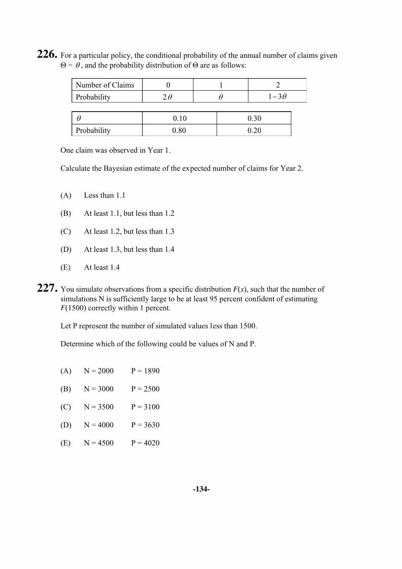
8/13/2019 Edu Exam c Sample Quest
http://slidepdf.com/reader/full/edu-exam-c-sample-quest 134/184
-134-
226. For a particular policy, the conditional probability of the annual number of claims givenΘ = θ , and the probability distribution of Θ are as follows:
Number of Claims 0 1 2
Probability 2θ θ 1 3θ −
θ 0.10 0.30
Probability 0.80 0.20
One claim was observed in Year 1.
Calculate the Bayesian estimate of the expected number of claims for Year 2.
(A)
Less than 1.1(B) At least 1.1, but less than 1.2
(C) At least 1.2, but less than 1.3
(D) At least 1.3, but less than 1.4
(E) At least 1.4
227. You simulate observations from a specific distribution F ( x), such that the number of
simulations N is sufficiently large to be at least 95 percent confident of estimatingF (1500) correctly within 1 percent.
Let P represent the number of simulated values less than 1500.
Determine which of the following could be values of N and P.
(A) N = 2000 P = 1890
(B) N = 3000 P = 2500
(C) N = 3500 P = 3100
(D) N = 4000 P = 3630
(E) N = 4500 P = 4020
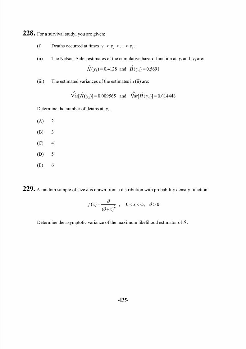
8/13/2019 Edu Exam c Sample Quest
http://slidepdf.com/reader/full/edu-exam-c-sample-quest 135/184
-135-
228. For a survival study, you are given:
(i) Deaths occurred at times 921 y y y <<< .
(ii) The Nelson-Aalen estimates of the cumulative hazard function at3
y and4 yare:
^ ^
3 4( ) 0.4128 and ( ) 0.5691 H y H y= =
(iii) The estimated variances of the estimates in (ii) are:
^
3Var[ ( )] 0.009565 H y =∧
and^
4Var[ ( )] 0.014448 H y =∧
Determine the number of deaths at 4 y .
(A) 2
(B) 3
(C) 4
(D) 5
(E) 6
229. A random sample of size n is drawn from a distribution with probability density function:
2( ) , 0 , 0
( ) f x x
x
θ θ
θ = < < ∞ >
+
Determine the asymptotic variance of the maximum likelihood estimator of θ .
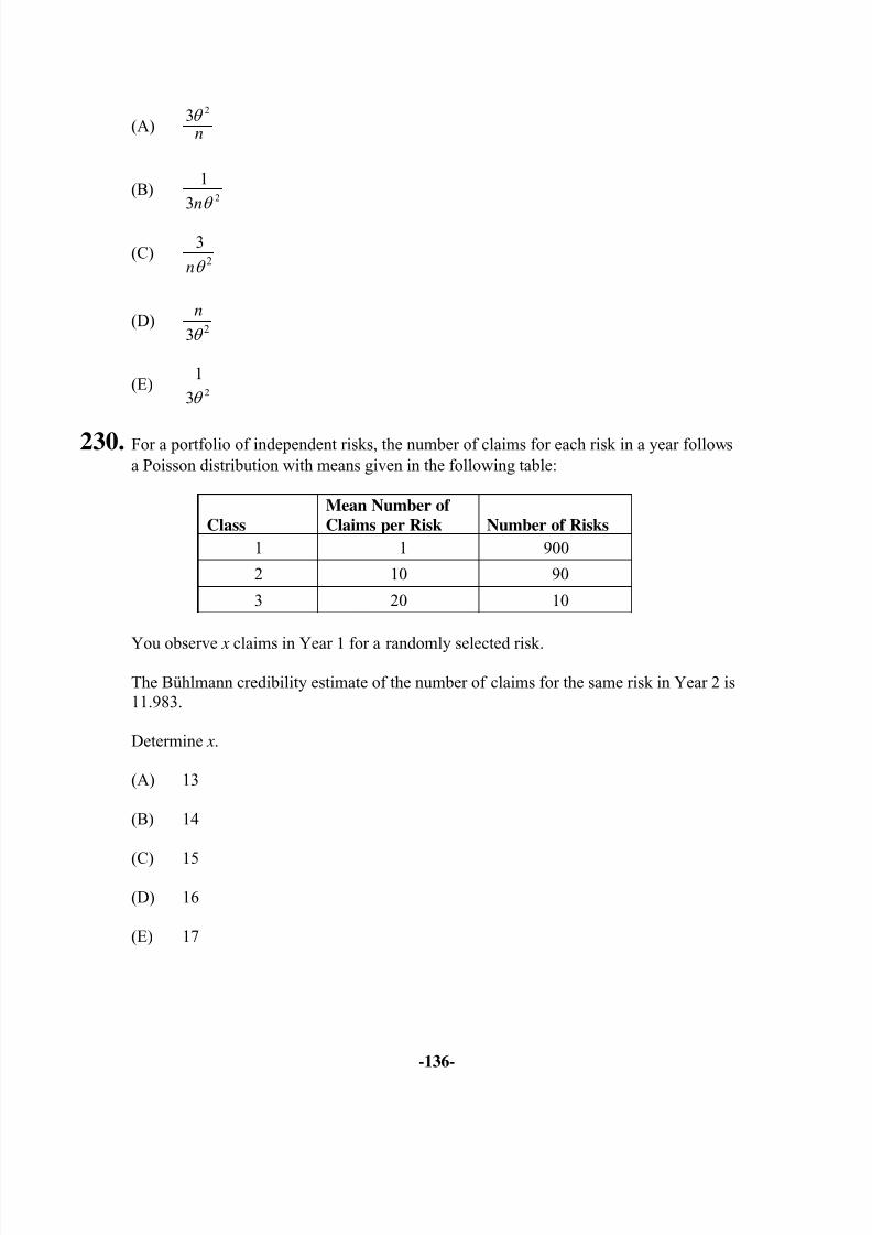
8/13/2019 Edu Exam c Sample Quest
http://slidepdf.com/reader/full/edu-exam-c-sample-quest 136/184
8/13/2019 Edu Exam c Sample Quest
http://slidepdf.com/reader/full/edu-exam-c-sample-quest 137/184
-137-
231. A survival study gave (0.283, 1.267) as the symmetric linear 95% confidence intervalfor H (5).
Using the delta method, determine the symmetric linear 95% confidence interval for S (5).
(A) (0.23, 0.69)
(B) (0.26, 0.72)
(C) (0.28, 0.75)
(D) (0.31, 0.73)
(E) (0.32, 0.80)
232. You are given:
(i) Losses on a certain warranty product in Year i follow a lognormal distributionwith parameters iµ and iσ .
(ii) iσ σ = , for i = 1, 2, 3,…
(iii) The parameters iµ vary in such a way that there is an annual inflation rate of 10%
for losses.
(iv) The following is a sample of seven losses:
Year 1: 20 40 50
Year 2: 30 40 90 120
Using trended losses, determine the method of moments estimate of 3µ .
(A) 3.87
(B) 4.00
(C) 30.00
(D) 55.71
(E) 63.01
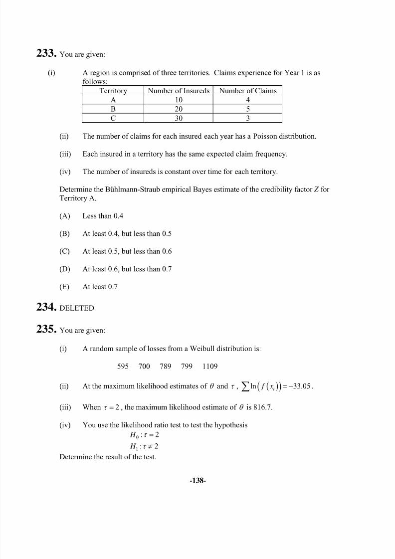
8/13/2019 Edu Exam c Sample Quest
http://slidepdf.com/reader/full/edu-exam-c-sample-quest 138/184
-138-
233. You are given:
(i) A region is comprised of three territories. Claims experience for Year 1 is asfollows:
Territory Number of Insureds Number of Claims
A 10 4B 20 5C 30 3
(ii) The number of claims for each insured each year has a Poisson distribution.
(iii) Each insured in a territory has the same expected claim frequency.
(iv) The number of insureds is constant over time for each territory.
Determine the Bühlmann-Straub empirical Bayes estimate of the credibility factor Z for
Territory A.
(A) Less than 0.4
(B) At least 0.4, but less than 0.5
(C) At least 0.5, but less than 0.6
(D) At least 0.6, but less than 0.7
(E) At least 0.7
234. DELETED
235. You are given:
(i) A random sample of losses from a Weibull distribution is:
595 700 789 799 1109
(ii) At the maximum likelihood estimates of θ and τ , ( )( )
ln 33.05i f x = −∑ .
(iii) When 2τ = , the maximum likelihood estimate of θ is 816.7.
(iv) You use the likelihood ratio test to test the hypothesis
0 : 2 H τ =
1 : 2 H τ ≠
Determine the result of the test.
8/13/2019 Edu Exam c Sample Quest
http://slidepdf.com/reader/full/edu-exam-c-sample-quest 139/184
-139-
(A) Do not reject 0 H at the 0.10 level of significance.
(B) Reject 0 H at the 0.10 level of significance, but not at the 0.05 level of
significance.
(C) Reject 0 H at the 0.05 level of significance, but not at the 0.025 level ofsignificance.
(D) Reject 0 H at the 0.025 level of significance, but not at the 0.01 level of
significance.
(E) Reject 0 H at the 0.01 level of significance.
236. For each policyholder, losses X 1,…, X n , conditional on Θ, are independently and
identically distributed with mean,
( ) ( )E , 1,2,..., j X j nµ θ θ = Θ = =
and variance,
( ) ( )Var , 1,2,..., jv X j nθ θ = Θ = = .
You are given:
(i) The Bühlmann credibility assigned for estimating X 5 based on X 1,…, X 4 is Z = 0.4.
(ii) The expected value of the process variance is known to be 8.
Calculate ( )Cov ,i j X X , i j≠ .
(A) Less than 0.5−
(B) At least 0.5− , but less than 0.5
(C) At least 0.5, but less than 1.5
(D) At least 1.5, but less than 2.5
(E) At least 2.5
8/13/2019 Edu Exam c Sample Quest
http://slidepdf.com/reader/full/edu-exam-c-sample-quest 140/184
-140-
237. Losses for a warranty product follow the lognormal distribution with underlying normalmean and standard deviation of 5.6 and 0.75 respectively.
You use simulation to estimate claim payments for a number of contracts with differentdeductibles.
The following are four uniform (0,1) random numbers:
0.6217 0.9941 0.8686 0.0485
Using these numbers and the inversion method, calculate the average payment per lossfor a contract with a deductible of 100.
(A) Less than 630
(B) At least 630, but less than 680
(C) At least 680, but less than 730
(D) At least 730, but less than 780
(E) At least 780
238. The random variable X has the exponential distribution with mean θ .
Calculate the mean-squared error of 2 X as an estimator of 2θ .
(A) 20 4θ
(B) 21 4θ
(C) 22 4θ
(D) 23 4θ
(E) 24 4θ
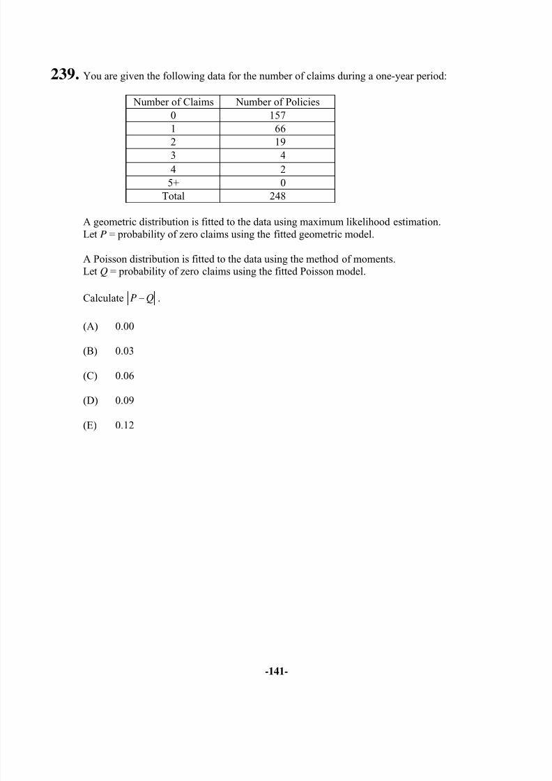
8/13/2019 Edu Exam c Sample Quest
http://slidepdf.com/reader/full/edu-exam-c-sample-quest 141/184
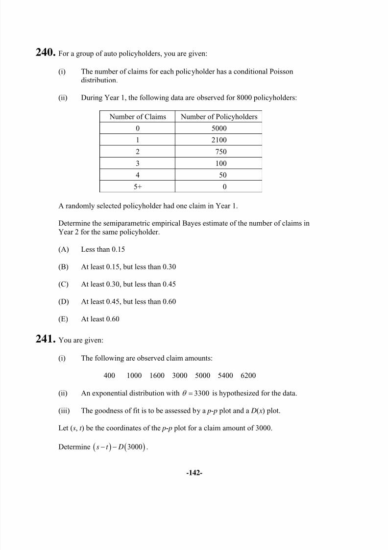
8/13/2019 Edu Exam c Sample Quest
http://slidepdf.com/reader/full/edu-exam-c-sample-quest 142/184
-142-
240. For a group of auto policyholders, you are given:
(i) The number of claims for each policyholder has a conditional Poissondistribution.
(ii) During Year 1, the following data are observed for 8000 policyholders:
Number of Claims Number of Policyholders
0 5000
1 2100
2 750
3 100
4 50
5+ 0
A randomly selected policyholder had one claim in Year 1.
Determine the semiparametric empirical Bayes estimate of the number of claims inYear 2 for the same policyholder.
(A) Less than 0.15
(B) At least 0.15, but less than 0.30
(C) At least 0.30, but less than 0.45
(D) At least 0.45, but less than 0.60
(E) At least 0.60
241. You are given:
(i) The following are observed claim amounts:
400 1000 1600 3000 5000 5400 6200
(ii) An exponential distribution with 3300θ = is hypothesized for the data.
(iii) The goodness of fit is to be assessed by a p- p plot and a D( x) plot.
Let (s, t ) be the coordinates of the p- p plot for a claim amount of 3000.
Determine ( ) ( )3000s t D− − .
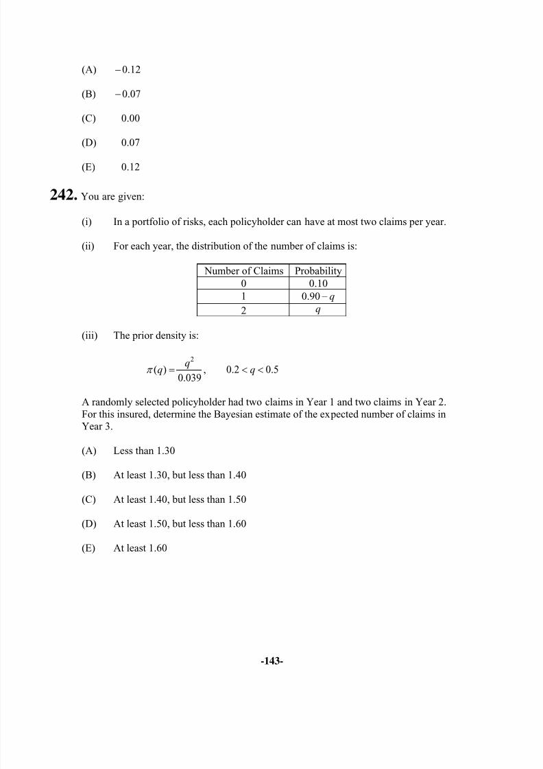
8/13/2019 Edu Exam c Sample Quest
http://slidepdf.com/reader/full/edu-exam-c-sample-quest 143/184
-143-
(A) − 0.12
(B) − 0.07
(C) 0.00
(D) 0.07
(E) 0.12
242. You are given:
(i) In a portfolio of risks, each policyholder can have at most two claims per year.
(ii) For each year, the distribution of the number of claims is:
Number of Claims Probability0 0.101 0.90 q−
2 q
(iii) The prior density is:
2
( ) , 0.2 0.50.039
qq qπ = < <
A randomly selected policyholder had two claims in Year 1 and two claims in Year 2.For this insured, determine the Bayesian estimate of the expected number of claims inYear 3.
(A) Less than 1.30
(B) At least 1.30, but less than 1.40
(C) At least 1.40, but less than 1.50
(D) At least 1.50, but less than 1.60
(E) At least 1.60
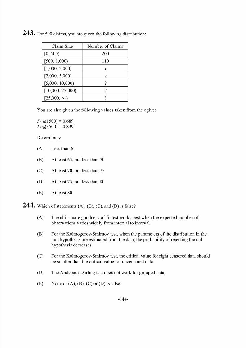
8/13/2019 Edu Exam c Sample Quest
http://slidepdf.com/reader/full/edu-exam-c-sample-quest 144/184
-144-
243. For 500 claims, you are given the following distribution:
Claim Size Number of Claims
[0, 500) 200
[500, 1,000) 110[1,000, 2,000) x
[2,000, 5,000) y
[5,000, 10,000) ?
[10,000, 25,000) ?
[25,000, ∞ ) ?
You are also given the following values taken from the ogive:
F 500(1500) = 0.689F 500(3500) = 0.839
Determine y.
(A) Less than 65
(B) At least 65, but less than 70
(C) At least 70, but less than 75
(D) At least 75, but less than 80
(E) At least 80
244. Which of statements (A), (B), (C), and (D) is false?
(A) The chi-square goodness-of-fit test works best when the expected number ofobservations varies widely from interval to interval.
(B) For the Kolmogorov-Smirnov test, when the parameters of the distribution in thenull hypothesis are estimated from the data, the probability of rejecting the null
hypothesis decreases.
(C) For the Kolmogorov-Smirnov test, the critical value for right censored data should be smaller than the critical value for uncensored data.
(D) The Anderson-Darling test does not work for grouped data.
(E) None of (A), (B), (C) or (D) is false.
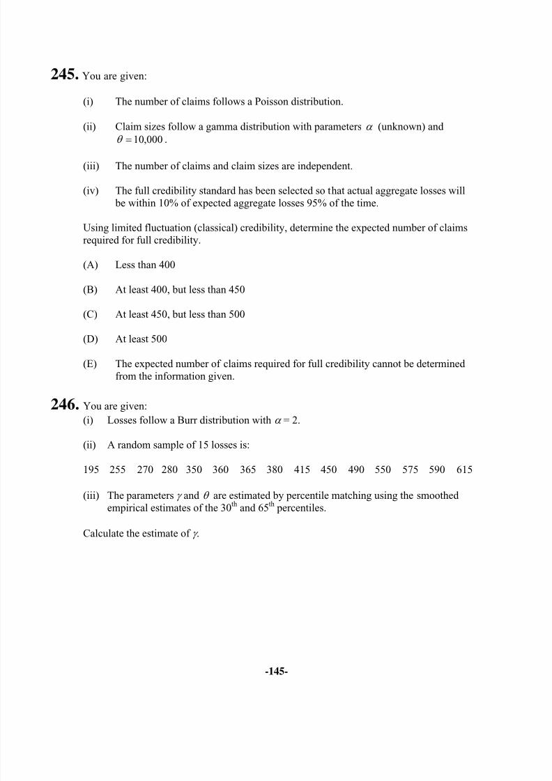
8/13/2019 Edu Exam c Sample Quest
http://slidepdf.com/reader/full/edu-exam-c-sample-quest 145/184
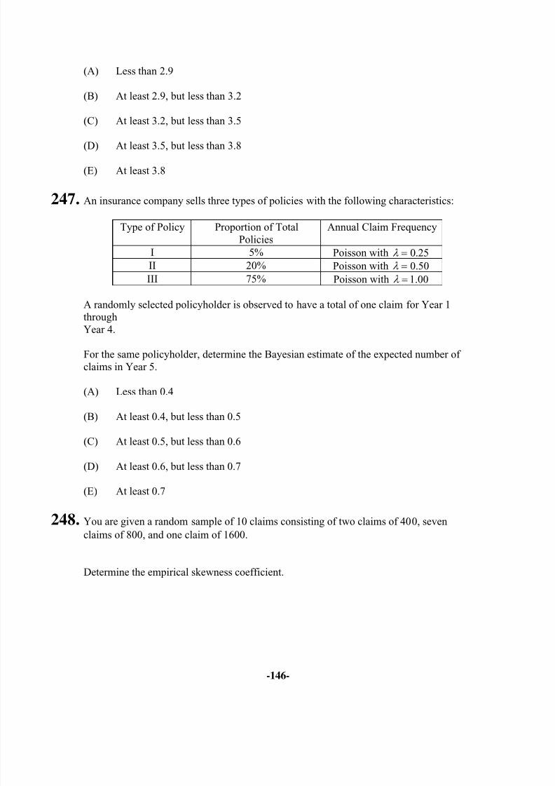
8/13/2019 Edu Exam c Sample Quest
http://slidepdf.com/reader/full/edu-exam-c-sample-quest 146/184
-146-
(A) Less than 2.9
(B) At least 2.9, but less than 3.2
(C) At least 3.2, but less than 3.5
(D) At least 3.5, but less than 3.8
(E) At least 3.8
247. An insurance company sells three types of policies with the following characteristics:
Type of Policy Proportion of TotalPolicies
Annual Claim Frequency
I 5% Poisson with 0.25λ = II 20% Poisson with 0.50λ =
III 75% Poisson with 1.00λ =
A randomly selected policyholder is observed to have a total of one claim for Year 1throughYear 4.
For the same policyholder, determine the Bayesian estimate of the expected number ofclaims in Year 5.
(A) Less than 0.4
(B) At least 0.4, but less than 0.5
(C) At least 0.5, but less than 0.6
(D) At least 0.6, but less than 0.7
(E) At least 0.7
248. You are given a random sample of 10 claims consisting of two claims of 400, sevenclaims of 800, and one claim of 1600.
Determine the empirical skewness coefficient.
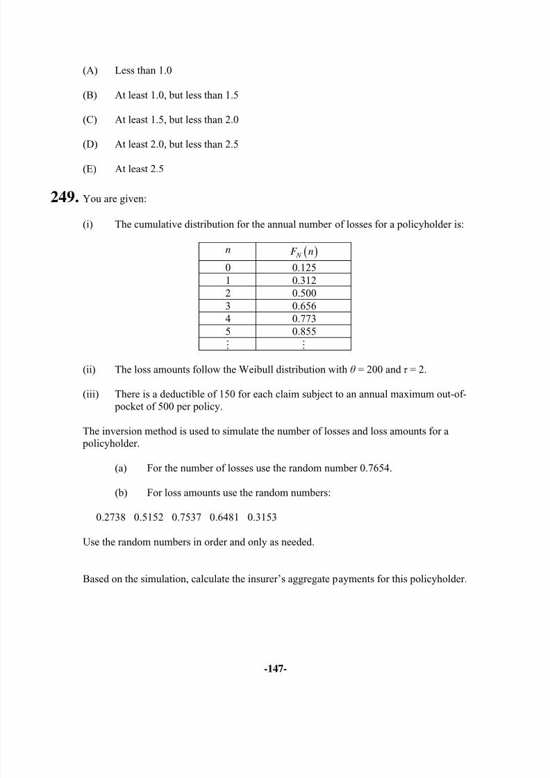
8/13/2019 Edu Exam c Sample Quest
http://slidepdf.com/reader/full/edu-exam-c-sample-quest 147/184
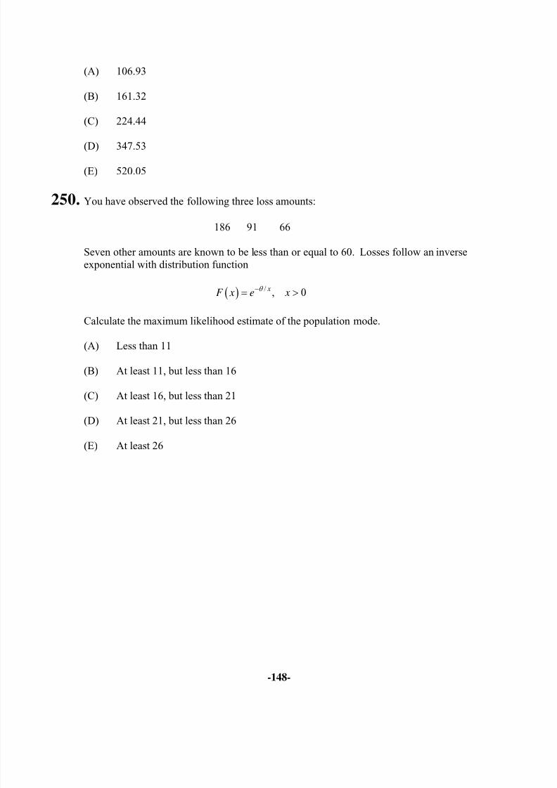
8/13/2019 Edu Exam c Sample Quest
http://slidepdf.com/reader/full/edu-exam-c-sample-quest 148/184
-148-
(A) 106.93
(B) 161.32
(C) 224.44
(D) 347.53
(E) 520.05
250. You have observed the following three loss amounts:
186 91 66
Seven other amounts are known to be less than or equal to 60. Losses follow an inverseexponential with distribution function
( ) / , 0 xF x e xθ −= >
Calculate the maximum likelihood estimate of the population mode.
(A) Less than 11
(B) At least 11, but less than 16
(C) At least 16, but less than 21
(D) At least 21, but less than 26
(E) At least 26
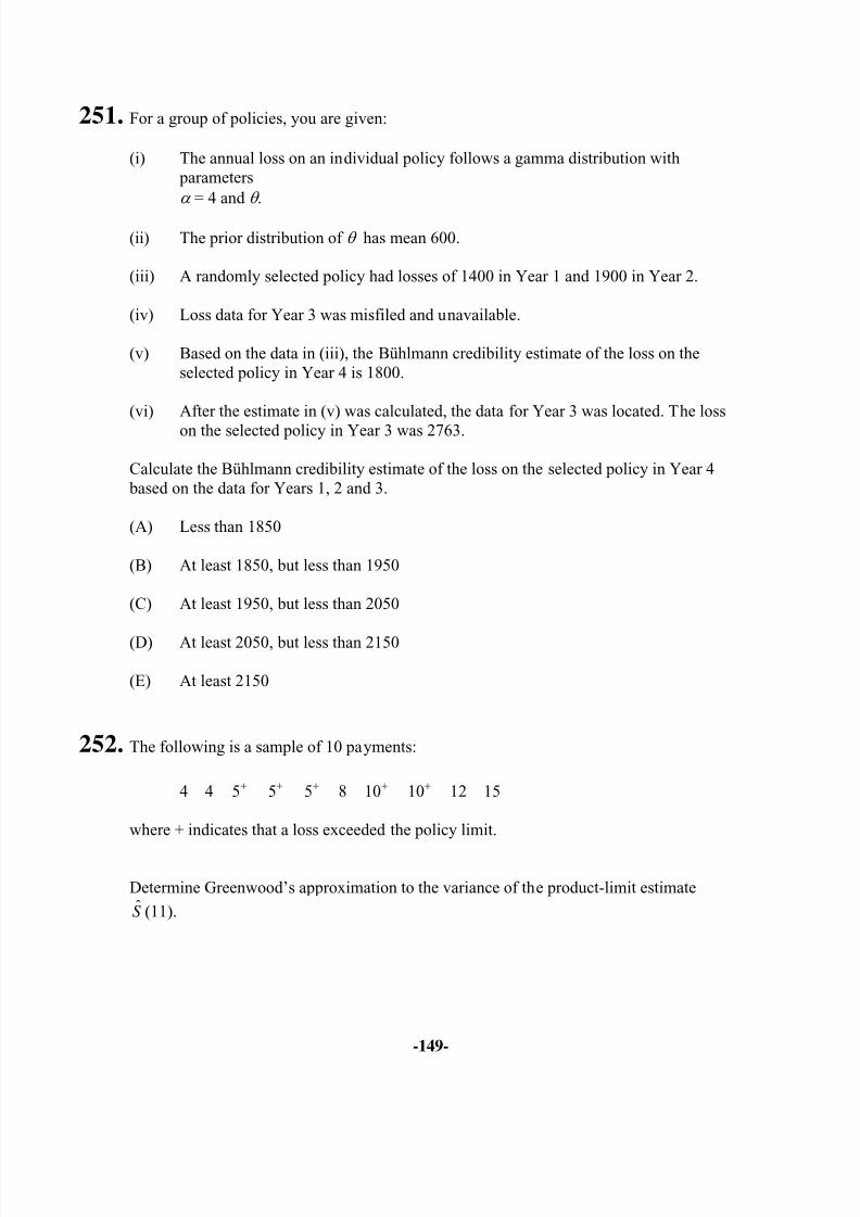
8/13/2019 Edu Exam c Sample Quest
http://slidepdf.com/reader/full/edu-exam-c-sample-quest 149/184
-149-
251. For a group of policies, you are given:
(i) The annual loss on an individual policy follows a gamma distribution with parametersα = 4 and θ .
(ii) The prior distribution of θ has mean 600.
(iii) A randomly selected policy had losses of 1400 in Year 1 and 1900 in Year 2.
(iv) Loss data for Year 3 was misfiled and unavailable.
(v) Based on the data in (iii), the Bühlmann credibility estimate of the loss on theselected policy in Year 4 is 1800.
(vi) After the estimate in (v) was calculated, the data for Year 3 was located. The loss
on the selected policy in Year 3 was 2763.
Calculate the Bühlmann credibility estimate of the loss on the selected policy in Year 4 based on the data for Years 1, 2 and 3.
(A) Less than 1850
(B) At least 1850, but less than 1950
(C) At least 1950, but less than 2050
(D) At least 2050, but less than 2150
(E) At least 2150
252. The following is a sample of 10 payments:
4 4 5+ 5+ 5+ 8 10+ 10+ 12 15
where + indicates that a loss exceeded the policy limit.
Determine Greenwood’s approximation to the variance of the product-limit estimate
S ˆ (11).
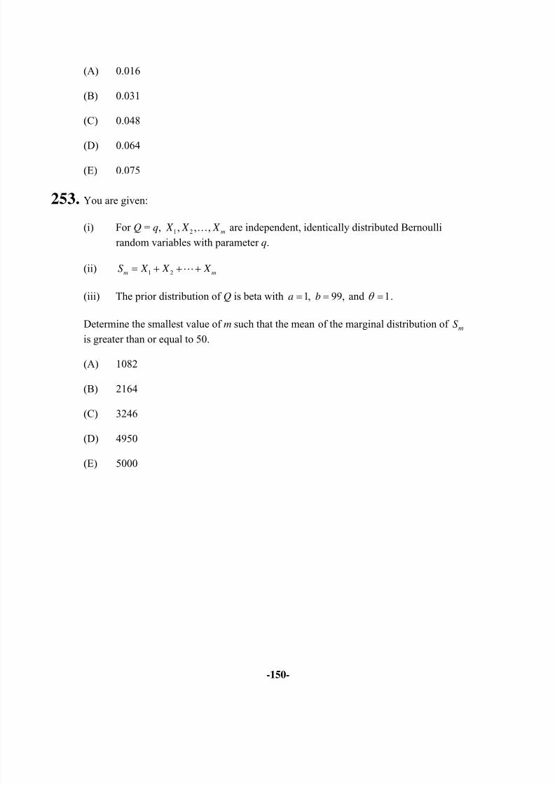
8/13/2019 Edu Exam c Sample Quest
http://slidepdf.com/reader/full/edu-exam-c-sample-quest 150/184
-150-
(A) 0.016
(B) 0.031
(C) 0.048
(D) 0.064
(E) 0.075
253. You are given:
(i) For Q = q, 1 2, , , m X X X are independent, identically distributed Bernoulli
random variables with parameter q.
(ii)1 2m m
S X X X = + + +
(iii) The prior distribution of Q is beta with 1, 99,a b= = and 1θ = .
Determine the smallest value of m such that the mean of the marginal distribution of mS
is greater than or equal to 50.
(A) 1082
(B) 2164
(C) 3246
(D) 4950
(E) 5000
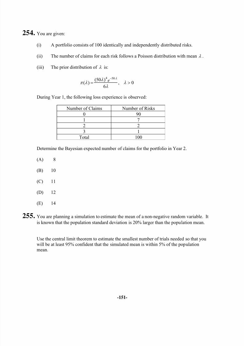
8/13/2019 Edu Exam c Sample Quest
http://slidepdf.com/reader/full/edu-exam-c-sample-quest 151/184
-151-
254. You are given:
(i) A portfolio consists of 100 identically and independently distributed risks.
(ii) The number of claims for each risk follows a Poisson distribution with mean λ .
(iii) The prior distribution of λ is:
4 50(50 )( ) , 0
6
e λ λ
π λ λ λ
−
= >
During Year 1, the following loss experience is observed:
Number of Claims Number of Risks0 90
1 72 23 1
Total 100
Determine the Bayesian expected number of claims for the portfolio in Year 2.
(A) 8
(B) 10
(C) 11
(D) 12
(E) 14
255. You are planning a simulation to estimate the mean of a non-negative random variable. Itis known that the population standard deviation is 20% larger than the population mean.
Use the central limit theorem to estimate the smallest number of trials needed so that youwill be at least 95% confident that the simulated mean is within 5% of the populationmean.
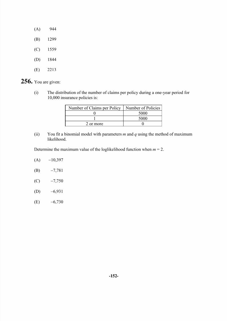
8/13/2019 Edu Exam c Sample Quest
http://slidepdf.com/reader/full/edu-exam-c-sample-quest 152/184
-152-
(A) 944
(B) 1299
(C) 1559
(D) 1844
(E) 2213
256. You are given:
(i) The distribution of the number of claims per policy during a one-year period for10,000 insurance policies is:
Number of Claims per Policy Number of Policies
0 50001 5000
2 or more 0
(ii) You fit a binomial model with parameters m and q using the method of maximumlikelihood.
Determine the maximum value of the loglikelihood function when m = 2.
(A) −10,397
(B) −7,781
(C) −7,750
(D) −6,931
(E) −6,730
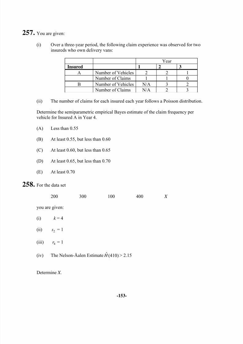
8/13/2019 Edu Exam c Sample Quest
http://slidepdf.com/reader/full/edu-exam-c-sample-quest 153/184
-153-
257. You are given:
(i) Over a three-year period, the following claim experience was observed for twoinsureds who own delivery vans:
YearInsured 1 2 3
A Number of Vehicles 2 2 1 Number of Claims 1 1 0
B Number of Vehicles N/A 3 2 Number of Claims N/A 2 3
(ii) The number of claims for each insured each year follows a Poisson distribution.
Determine the semiparametric empirical Bayes estimate of the claim frequency pervehicle for Insured A in Year 4.
(A) Less than 0.55
(B) At least 0.55, but less than 0.60
(C) At least 0.60, but less than 0.65
(D) At least 0.65, but less than 0.70
(E) At least 0.70
258. For the data set
200 300 100 400 X
you are given:
(i) k = 4
(ii) 2s = 1
(iii) 4r = 1
(iv) The Nelson-Åalen Estimate ˆ (410) H > 2.15
Determine X .
8/13/2019 Edu Exam c Sample Quest
http://slidepdf.com/reader/full/edu-exam-c-sample-quest 154/184
-154-
(A) 100
(B) 200
(C) 300
(D) 400
(E) 500
259. You are given:
(i) A hospital liability policy has experienced the following numbers of claims over a10-year period:
10 2 4 0 6 2 4 5 4 2
(ii) Numbers of claims are independent from year to year.
(iii) You use the method of maximum likelihood to fit a Poisson model.
Determine the estimated coefficient of variation of the estimator of the Poisson parameter.
(A) 0.10
(B) 0.16
(C) 0.22
(D) 0.26
(E) 1.00
260. You are given:
(i) Claim sizes follow an exponential distribution with mean θ .
(ii) For 80% of the policies, θ = 8.
(iii) For 20% of the policies, 2θ = .
A randomly selected policy had one claim in Year 1 of size 5.
Calculate the Bayesian expected claim size for this policy in Year 2.
8/13/2019 Edu Exam c Sample Quest
http://slidepdf.com/reader/full/edu-exam-c-sample-quest 155/184
-155-
(A) Less than 5.8
(B) At least 5.8, but less than 6.2
(C) At least 6.2, but less than 6.6
(D) At least 6.6, but less than 7.0
(E) At least 7.0
261. DELETED
262. You are given:
(i) At time 4 hours, there are 5 working light bulbs.
(ii) The 5 bulbs are observed for p more hours.
(iii) Three light bulbs burn out at times 5, 9, and 13 hours, while the remaining light bulbs are still working at time 4 + p hours.
(iv) The distribution of failure times is uniform on ( )0,ω .
(v) The maximum likelihood estimate of ω is 29.
Determine p.
(A) Less than 10
(B) At least 10, but less than 12
(C) At least 12, but less than 14
(D) At least 14, but less than 16
(E) At least 16
8/13/2019 Edu Exam c Sample Quest
http://slidepdf.com/reader/full/edu-exam-c-sample-quest 156/184
-156-
263. You are given:
(i) The number of claims incurred in a month by any insured follows a Poissondistribution with mean λ .
(ii) The claim frequencies of different insureds are independent.
(iii) The prior distribution of λ is Weibull with 0.1θ = and 2τ = .
(iv) Some values of the gamma function are
( ) ( ) ( ) ( )0.5 1.77245, 1 1, 1.5 0.88623, 2 1Γ = Γ = Γ = Γ =
(v) Month Number of Insureds Number of Claims
1 100 102 150 113 250 14
Determine the Bühlmann-Straub credibility estimate of the number of claims in the next12 months for 300 insureds.
(A) Less than 255
(B) At least 255, but less than 275
(C) At least 275, but less than 295
(D) At least 295, but less than 315
(E) At least 315
8/13/2019 Edu Exam c Sample Quest
http://slidepdf.com/reader/full/edu-exam-c-sample-quest 157/184
-157-
264. You are given:
(i) The following data set:
2500 2500 2500 3617 3662 4517 5000 5000 6010 6932 7500 7500
(ii)^
1(7000) H is the Nelson-Åalen estimate of the cumulative hazard rate function
calculated under the assumption that all of the observations in (i) are uncensored.
(iii)^
2(7000) H is the Nelson-Åalen estimate of the cumulative hazard rate function
calculated under the assumption that all occurrences of the values 2500, 5000 and7500 in (i) reflect right-censored observations and that the remaining observedvalues are uncensored.
Calculate| ^ ^1 2(7000) (7000) H H − |.
(A) Less than 0.1
(B) At least 0.1, but less than 0.3
(C) At least 0.3, but less than 0.5
(D) At least 0.5, but less than 0.7
(E) At least 0.7
8/13/2019 Edu Exam c Sample Quest
http://slidepdf.com/reader/full/edu-exam-c-sample-quest 158/184
-158-
265. For a warranty product you are given:
(i) Paid losses follow the lognormal distribution with 13.294µ = and 0.494σ = .
(ii) The ratio of estimated unpaid losses to paid losses, y, is modeled by
0.851 0.7470.801 x y x e−=
where
x = 2006 − contract purchase year
The inversion method is used to simulate four paid losses with the following four uniform(0,1) random numbers:
0.2877 0.1210 0.8238 0.6179
Using the simulated values, calculate the empirical estimate of the average unpaid lossesfor purchase year 2005.
(A) Less than 300,000
(B) At least 300,000, but less than 400,000
(C) At least 400,000, but less than 500,000
(D) At least 500,000, but less than 600,000(E) At least 600,000
266. Five models are fitted to a sample of n = 260 observations with the following results:
Model Number of Parameters LoglikelihoodI 1 − 414II 2 − 412III 3 − 411IV 4 − 409
V 6 − 409
Determine the model favored by the Schwarz Bayesian criterion.
8/13/2019 Edu Exam c Sample Quest
http://slidepdf.com/reader/full/edu-exam-c-sample-quest 159/184
8/13/2019 Edu Exam c Sample Quest
http://slidepdf.com/reader/full/edu-exam-c-sample-quest 160/184
-160-
(A) 0.377
(B) 0.400
(C) 0.417
(D) 0.439
(E) 0.485
269. The random variables 1 2, , , n X X X are independent and identically distributed with
probability density function
/
( ) , 0 x
e f x x
θ
θ
−
= ≥
Determine 2 E X .
(A) 21n
nθ
+
(B) 2
2
1n
nθ
+
(C)
2
n
θ
(D)2
n
θ
(E) 2θ
270. Three individual policyholders have the following claim amounts over four years:
Policyholder Year 1 Year 2 Year 3 Year 4X 2 3 3 4Y 5 5 4 6Z 5 5 3 3
Using the nonparametric empirical Bayes procedure, calculate the estimated variance ofthe hypothetical means.
8/13/2019 Edu Exam c Sample Quest
http://slidepdf.com/reader/full/edu-exam-c-sample-quest 161/184
-161-
(A) Less than 0.40
(B) At least 0.40, but less than 0.60
(C) At least 0.60, but less than 0.80
(D) At least 0.80, but less than 1.00
(E) At least 1.00
271. DELETED
272. You are given:
(i) The number of claims made by an individual in any given year has a binomial
distribution with parameters m = 4 and q.(ii) The prior distribution of q has probability density function
( ) 6 (1 ), 0 1q q q qπ = − < < .
(iii) Two claims are made in a given year.
Determine the mode of the posterior distribution of q.
(A) 0.17
(B) 0.33
(C) 0.50
(D) 0.67
(E) 0.83
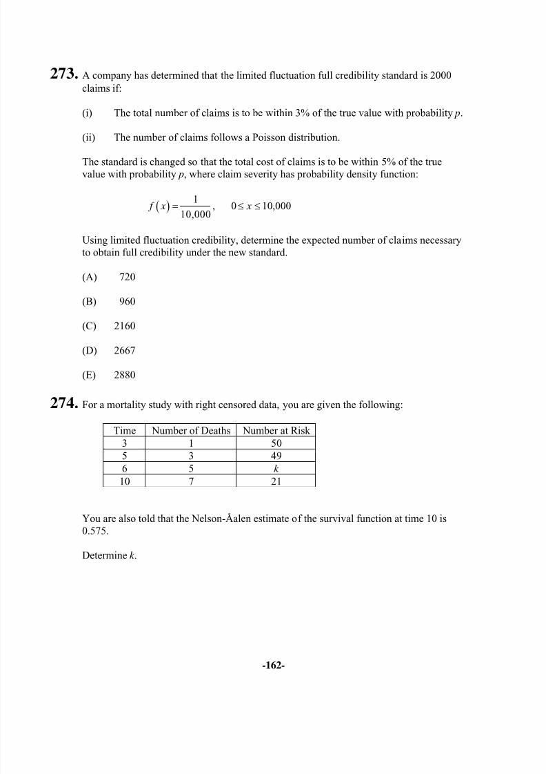
8/13/2019 Edu Exam c Sample Quest
http://slidepdf.com/reader/full/edu-exam-c-sample-quest 162/184
-162-
273. A company has determined that the limited fluctuation full credibility standard is 2000claims if:
(i) The total number of claims is to be within 3% of the true value with probability p.
(ii) The number of claims follows a Poisson distribution.
The standard is changed so that the total cost of claims is to be within 5% of the truevalue with probability p, where claim severity has probability density function:
( )1
10,000 f x = , 0 000,10≤≤ x
Using limited fluctuation credibility, determine the expected number of claims necessaryto obtain full credibility under the new standard.
(A) 720
(B) 960
(C) 2160
(D) 2667
(E) 2880
274. For a mortality study with right censored data, you are given the following:
Time Number of Deaths Number at Risk3 1 505 3 496 5 k
10 7 21
You are also told that the Nelson-Åalen estimate of the survival function at time 10 is0.575.
Determine k .
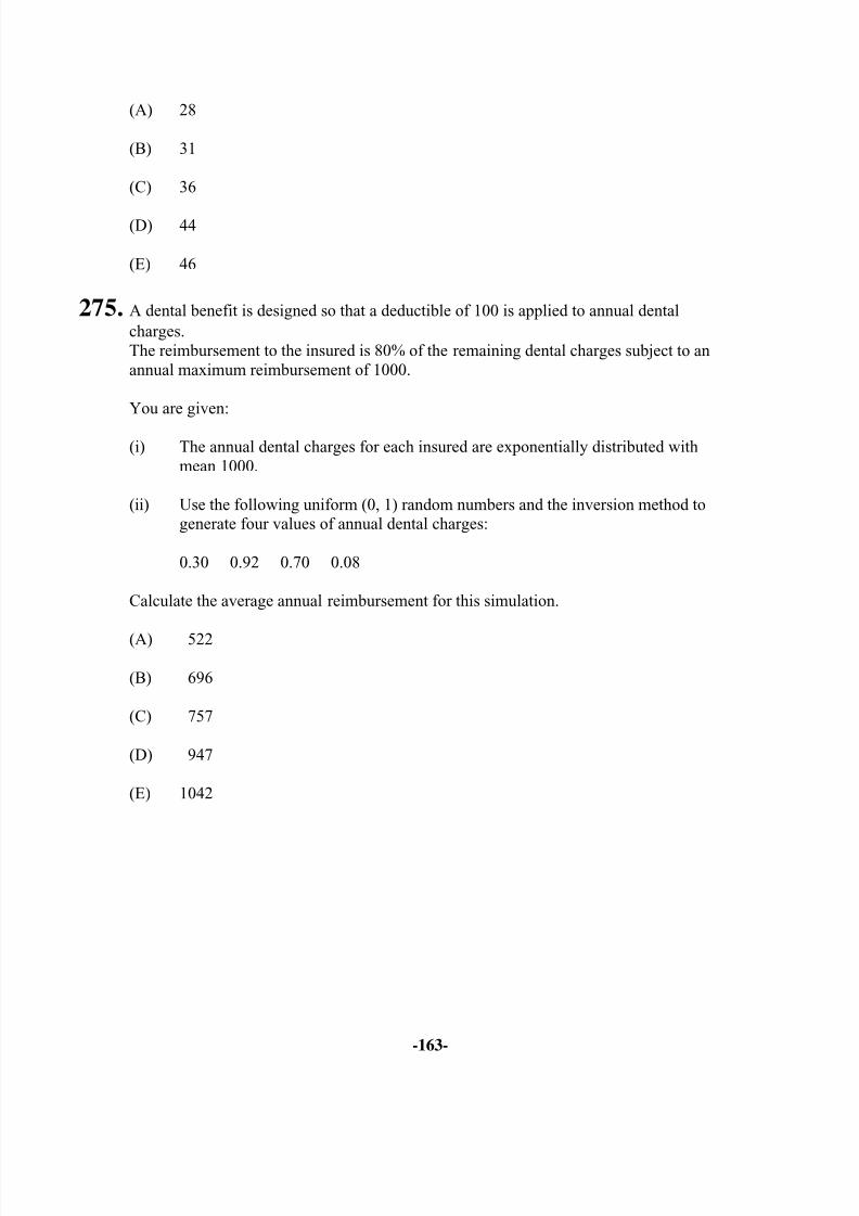
8/13/2019 Edu Exam c Sample Quest
http://slidepdf.com/reader/full/edu-exam-c-sample-quest 163/184
-163-
(A) 28
(B) 31
(C) 36
(D) 44
(E) 46
275. A dental benefit is designed so that a deductible of 100 is applied to annual dentalcharges.The reimbursement to the insured is 80% of the remaining dental charges subject to anannual maximum reimbursement of 1000.
You are given:
(i) The annual dental charges for each insured are exponentially distributed withmean 1000.
(ii) Use the following uniform (0, 1) random numbers and the inversion method togenerate four values of annual dental charges:
0.30 0.92 0.70 0.08
Calculate the average annual reimbursement for this simulation.
(A) 522
(B) 696
(C) 757
(D) 947
(E) 1042
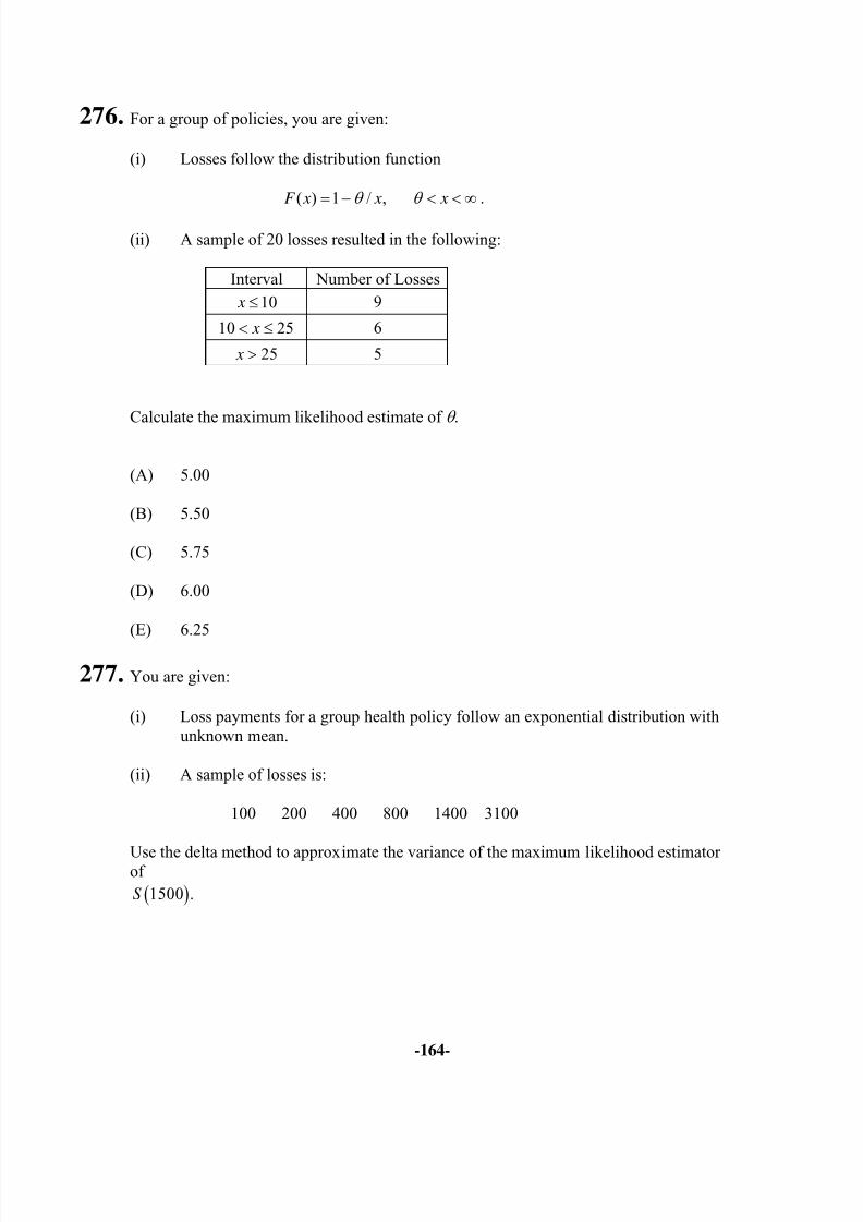
8/13/2019 Edu Exam c Sample Quest
http://slidepdf.com/reader/full/edu-exam-c-sample-quest 164/184
-164-
276. For a group of policies, you are given:
(i) Losses follow the distribution function
( ) 1 / ,F x x xθ θ = − < < ∞ .
(ii) A sample of 20 losses resulted in the following:
Interval Number of Losses
10 x ≤ 9
10 25 x< ≤ 6
25 x > 5
Calculate the maximum likelihood estimate of θ .
(A) 5.00
(B) 5.50
(C) 5.75
(D) 6.00
(E) 6.25
277. You are given:
(i) Loss payments for a group health policy follow an exponential distribution withunknown mean.
(ii) A sample of losses is:
100 200 400 800 1400 3100
Use the delta method to approximate the variance of the maximum likelihood estimatorof
( )1500 .S
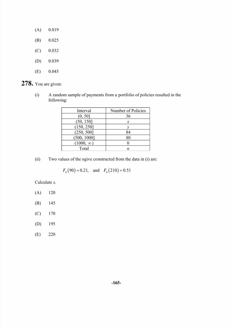
8/13/2019 Edu Exam c Sample Quest
http://slidepdf.com/reader/full/edu-exam-c-sample-quest 165/184
-165-
(A) 0.019
(B) 0.025
(C) 0.032
(D) 0.039
(E) 0.045
278. You are given:
(i) A random sample of payments from a portfolio of policies resulted in thefollowing:
Interval Number of Policies
(0, 50] 36(50, 150] x
(150, 250] y
(250, 500] 84(500, 1000] 80(1000, ∞ ) 0
Total n
(ii) Two values of the ogive constructed from the data in (i) are:
( )90 0.21,
nF = and
( )210 0.51
nF =
Calculate x.
(A) 120
(B) 145
(C) 170
(D) 195
(E) 220
8/13/2019 Edu Exam c Sample Quest
http://slidepdf.com/reader/full/edu-exam-c-sample-quest 166/184
-166-
279. Loss amounts have the distribution function
( ) ( )
2/100 , 0 100
1 , 100
x xF x
x
≤ ≤=
<
An insurance pays 80% of the amount of the loss in excess of an ordinary deductible of20, subject to a maximum payment of 60 per loss.
Calculate the conditional expected claim payment, given that a payment has been made.
(A) 37
(B) 39
(C) 43
(D) 47
(E) 49
280. A compound Poisson claim distribution has 5λ = and individual claim amountsdistributed as follows:
x ( ) X f x
5 0.6
k 0.4 where 5k >
The expected cost of an aggregate stop-loss insurance subject to a deductible of 5 is28.03.
Calculate k .
(A) 6
(B) 7
(C) 8
(D) 9
(E) 10
8/13/2019 Edu Exam c Sample Quest
http://slidepdf.com/reader/full/edu-exam-c-sample-quest 167/184
-167-
281. For a special investment product, you are given:
(i) All deposits are credited with 75% of the annual equity index return, subject to aminimum guaranteed crediting rate of 3%.
(ii) The annual equity index return is normally distributed with a mean of 8% and astandard deviation of 16%.
(iii) For a random variable X which has a normal distribution with mean µ and
standard deviation σ , you are given the following limited expected values:
[ ]3% E X ∧
6%µ = 8%µ =
12%σ = − 0.43% 0.31%16%σ = − 1.99% − 1.19%
[ ]4% E X ∧
6%µ = 8%µ =
12%σ = 0.15% 0.95%16%σ = − 1.43% − 0.58%
Calculate the expected annual crediting rate.
(A) 8.9%
(B) 9.4%
(C) 10.7%
(D) 11.0%
(E) 11.6%
8/13/2019 Edu Exam c Sample Quest
http://slidepdf.com/reader/full/edu-exam-c-sample-quest 168/184
8/13/2019 Edu Exam c Sample Quest
http://slidepdf.com/reader/full/edu-exam-c-sample-quest 169/184
-169-
284. A risk has a loss amount which has a Poisson distribution with mean 3.
An insurance covers the risk with an ordinary deductible of 2. An alternative insurancereplaces the deductible with coinsurance α , which is the proportion of the loss paid bythe insurance, so that the expected insurance cost remains the same.
Calculate α .
(A) 0.22
(B) 0.27
(C) 0.32
(D) 0.37
(E) 0.42
285. You are the producer for the television show Actuarial Idol. Each year, 1000 actuarialclubs audition for the show. The probability of a club being accepted is 0.20.
The number of members of an accepted club has a distribution with mean 20 andvariance 20. Club acceptances and the numbers of club members are mutuallyindependent.
Your annual budget for persons appearing on the show equals 10 times the expected
number of persons plus 10 times the standard deviation of the number of persons.Calculate your annual budget for persons appearing on the show.
(A) 42,600
(B) 44,200
(C) 45,800
(D) 47,400
(E) 49,000
8/13/2019 Edu Exam c Sample Quest
http://slidepdf.com/reader/full/edu-exam-c-sample-quest 170/184
-170-
286. Michael is a professional stuntman who performs dangerous motorcycle jumps atextreme sports events around the world.
The annual cost of repairs to his motorcycle is modeled by a two parameter Paretodistribution with 5000θ = and 2α = .
An insurance reimburses Michael’s motorcycle repair costs subject to the following provisions:
(i) Michael pays an annual ordinary deductible of 1000 each year.
(ii) Michael pays 20% of repair costs between 1000 and 6000 each year.
(iii) Michael pays 100% of the annual repair costs above 6000 until Michael has paid10,000 in out-of-pocket repair costs each year.
(iv) Michael pays 10% of the remaining repair costs each year.
Calculate the expected annual insurance reimbursement.
(A) 2300
(B) 2500
(C) 2700
(D) 2900
(E) 3100
287. For an aggregate loss distribution S :
(i) The number of claims has a negative binomial distribution with r = 16 and 6 β = .
(ii) The claim amounts are uniformly distributed on the interval (0, 8).
(iii) The number of claims and claim amounts are mutually independent.
Using the normal approximation for aggregate losses, calculate the premium such that the probability that aggregate losses will exceed the premium is 5%.
8/13/2019 Edu Exam c Sample Quest
http://slidepdf.com/reader/full/edu-exam-c-sample-quest 171/184
-171-
(A) 500
(B) 520
(C) 540
(D) 560
(E) 580
288. The random variable N has a mixed distribution:
(i) With probability p, N has a binomial distribution with 0.5q = and 2m = .
(ii) With probability 1 p− , N has a binomial distribution with 0.5q = and 4m = .
Which of the following is a correct expression for ( )Prob 2 N = ?
(A) 20.125 p
(B) 0.375 0.125 p+
(C) 20.375 0.125 p+
(D) 2
0.375 0.125 p−
(E) 0.375 0.125 p−
289. A compound Poisson distribution has 5λ = and claim amount distribution as follows:
x ( ) p x
100 0.80
500 0.16
1000 0.04
Calculate the probability that aggregate claims will be exactly 600.
8/13/2019 Edu Exam c Sample Quest
http://slidepdf.com/reader/full/edu-exam-c-sample-quest 172/184
-172-
(A) 0.022
(B) 0.038
(C) 0.049
(D) 0.060
(E) 0.070
290. A random variable X has a two-point mixture distribution with pdf
/2 /31 1( ) , 0
8 4
x x f x e e x
− −= + ≥ .
You are to simulate one value, x, from this distribution using uniform random numbers0.2 and 0.6. Use the value 0.2 and the inversion method to simulate J where J = 1 refersto the first random variable in the mixture and J = 2 refers to the second random variable.
Then use 0.6 and the inversion method to simulate a value from X .
Calculate the value of x.
(A) 0.45
(B) 1.02
(C) 1.53
(D) 1.83
(E) 2,75
291. There are four decrements, labeled (1), (2), (3), and (4). Over the next year the probabilities for each are 0.05, 0.10, 0.15, and 0.20, respectively. There are 500independent lives subject to these decrements. You plan to simulate the results for thenext year using successive binomial distributions and do so in the order in which thedecrements are numbered. The first binomial simulation had 23 instances of decrement(1) and the second binomial simulation had 59 instances of decrement (2).
Determine the values of m and q for the binomial distribution to be used for simulatingdecrement (3).
8/13/2019 Edu Exam c Sample Quest
http://slidepdf.com/reader/full/edu-exam-c-sample-quest 173/184
-173-
(A) m = 500, q = 0.15
(B) m = 500, q = 0.21
(C) m = 418, q = 0.15
(D) m = 418, q = 0.18
(E) m = 418, q = 0.21
292-295. Use the following information for questions 292-295.
Four of XYZ’s policyholders have the following history.
Policynumber
Date of birth Date policyissued
Status on12-31-2012
Status on policy
anniversary in2013
1 4-1-1930 3-1-1980 Died 10-1-2012
Died10-1-2012
2 7-1-1930 10-1-1990 Insured Surrendered5-1-2013
3 8-1-1930 1-1-2000 Insured Insured4 9-1-1930 8-1-2000 Surrendered
11-1-2012Surrendered11-1-2012
292. XYZ conducts a mortality study from 1-1-2012 through 12-31-2012 using actual ages.
Calculate the absolute value of the difference between the estimated mortality probabilities at age 82, using the exact and actuarial methods.
(A) 0.012
(B) 0.015
(C) 0.018
(D) 0.021
(E) 0.024
8/13/2019 Edu Exam c Sample Quest
http://slidepdf.com/reader/full/edu-exam-c-sample-quest 174/184
-174-
293. XYZ conducts a mortality study from 1-1-2012 through 12-31-2012 using insuring ages.
XYZ assigns insuring ages based on the age at the nearest birthday when the policy isissued.
Calculate the absolute value of the difference between the estimated mortality probabilities at age 82, using the exact and actuarial methods.
(A) 0.046
(B) 0.051
(C) 0.055
(D) 0.060
(E) 0.064
294. XYZ conducts a mortality study from anniversaries in 2012 through anniversaries in2013 using insuring ages.
XYZ assigns insuring ages based on the age at the nearest birthday when the policy isissued.
Calculate the absolute value of the difference between the estimated mortality probabilities at age 82, using the exact and actuarial methods.
(A) 0.031
(B) 0.035
(C) 0.039
(D) 0.042
(E) 0.045
8/13/2019 Edu Exam c Sample Quest
http://slidepdf.com/reader/full/edu-exam-c-sample-quest 175/184
-175-
295. Estimate the variance of the estimator based on exact exposures from Question 293 usingthe delta method approach.
(A) 0.13
(B) 0.26
(C) 0.41
(D) 0.56
(E) 0.71
296-297. Use the following information for questions 296-297.
A mortality study of insured lives is being conducted. Insuring ages are employed and thestudy runs from anniversaries in 2010 through anniversaries in 2012. Assume that eventsthat can occur between anniversaries do so uniformly. The following was observed:
There are 10,000 lives at age 60 when first observed in 2010. Between then and their nextanniversary 100 die and 800 surrender their policy. In 2011, 1000 new policies are sold atage 61. For those insured at their age 61 anniversary in 2011, 120 die and 700 surrender before their 2012 anniversary.
There are 8000 lives at age 61 when first observed in 2010. Between then and their nextanniversary 80 die and 700 surrender their policy. In 2011, 800 new policies are sold atage 62. For those insured at their age 62 anniversary in 2011, 90 die and 600 surrender before their 2012 anniversary.
296. Determine the actuarial estimate of the mortality probability at age 61.
(A) 0.0112
(B) 0.0113
(C) 0.0114
(D) 0.0115
(E) 0.0116
8/13/2019 Edu Exam c Sample Quest
http://slidepdf.com/reader/full/edu-exam-c-sample-quest 176/184
-176-
297. Determine the estimate base on exact exposures of the mortality probability at age 61.
(A) 0.0112
(B) 0.0113
(C) 0.0114
(D) 0.0115
(E) 0.0116
298. For a warranty policy, the expenses, E , are the product of the random variable Y and theloss amount, X . That is, E = XY. Loss amounts, X , follow the lognormal distribution withthe underlying normal distribution parameters µ = 5.2 and σ = 1.4. Given X , the
conditional probability density function of Y is:
/2( | ) , 02
y x x f y x e y
−= >
Use the inversion method and the following three uniform (0, 1) random numbers tosimulate three loss amounts:
0.937 0.512 0.281
For each simulated loss amount, use the following uniform (0, 1) random numbers, inorder, to simulate three expense amounts.
0.433 0.298 0.978
Calculate the average value of expenses based on the three simulated amounts.
(A) Less than 23
(B) At least 23, but less than 28
(C) At least 28, but less than 33
(D) At least 33, but less than 38
(E) At least 38
8/13/2019 Edu Exam c Sample Quest
http://slidepdf.com/reader/full/edu-exam-c-sample-quest 177/184
-177-
299. For a health insurance policy effective January 1, the number of claims in a one-year period follows the Poisson distribution with mean λ = 5.
The following uniform (0, 1) random numbers are used in the given order to simulate thetime of the first claim and the times between occurrences of subsequent claims.
0.605 0.529 0.782
Calculate the simulated date of occurrence of the third claim.
(A) Before May 1
(B) On or after May 1, but before August 15
(C) On or after August 15, but before September 1
(D) On or after September 1, but before September 30
(E) On or after September 30
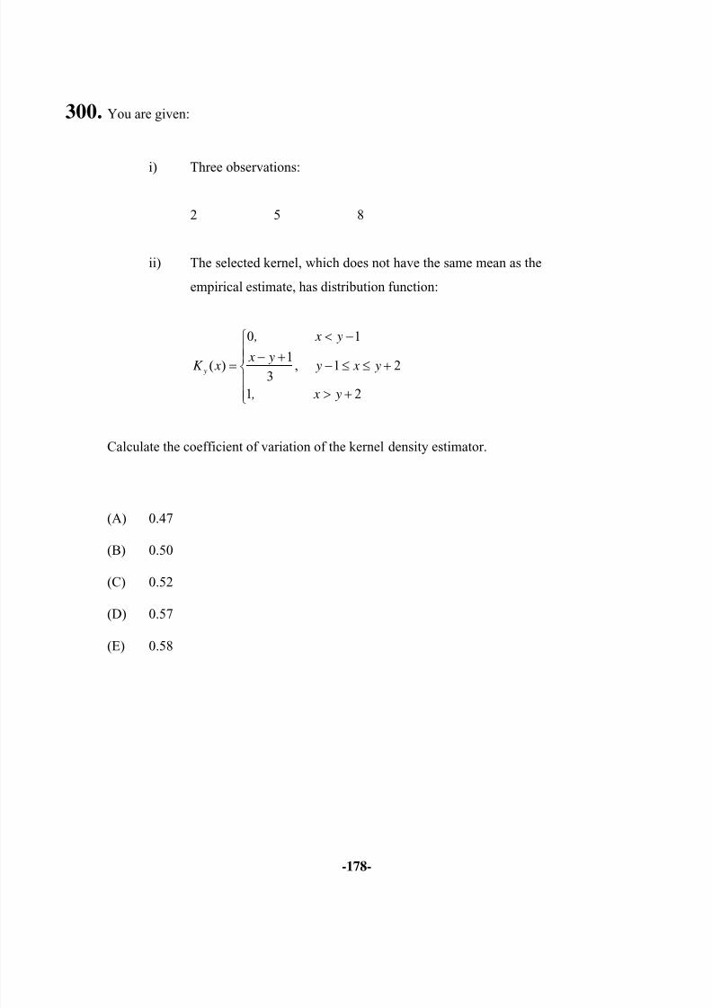
8/13/2019 Edu Exam c Sample Quest
http://slidepdf.com/reader/full/edu-exam-c-sample-quest 178/184
-178-
300. You are given:
i) Three observations:
2 5 8
ii) The selected kernel, which does not have the same mean as the
empirical estimate, has distribution function:
0 1
1( ) , 1 23
1 2
y
, x y
x yK x y x y
, x y
< −
− += − ≤ ≤ +
> +
Calculate the coefficient of variation of the kernel density estimator.
(A) 0.47
(B) 0.50
(C) 0.52
(D) 0.57
(E) 0.58
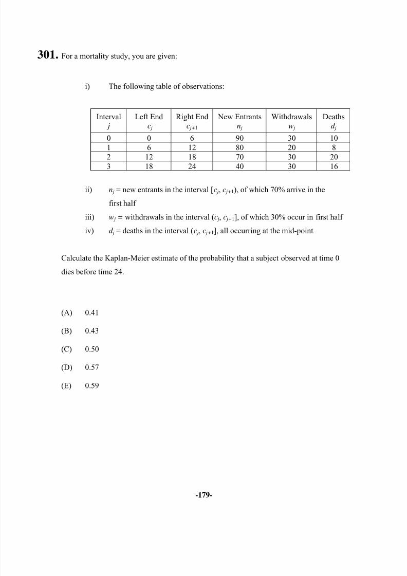
8/13/2019 Edu Exam c Sample Quest
http://slidepdf.com/reader/full/edu-exam-c-sample-quest 179/184
-179-
301. For a mortality study, you are given:
i) The following table of observations:
Interval j
Left Endc j
Right Endc j+1
New Entrantsn j
Withdrawalsw j
Deathsd j
0 0 6 90 30 101 6 12 80 20 82 12 18 70 30 203 18 24 40 30 16
ii) n j = new entrants in the interval [c j, c j+1), of which 70% arrive in the
first half
iii) w j = withdrawals in the interval (c j, c j+1], of which 30% occur in first half
iv) d j = deaths in the interval (c j, c j+1], all occurring at the mid-point
Calculate the Kaplan-Meier estimate of the probability that a subject observed at time 0
dies before time 24.
(A) 0.41
(B) 0.43
(C) 0.50
(D) 0.57
(E) 0.59
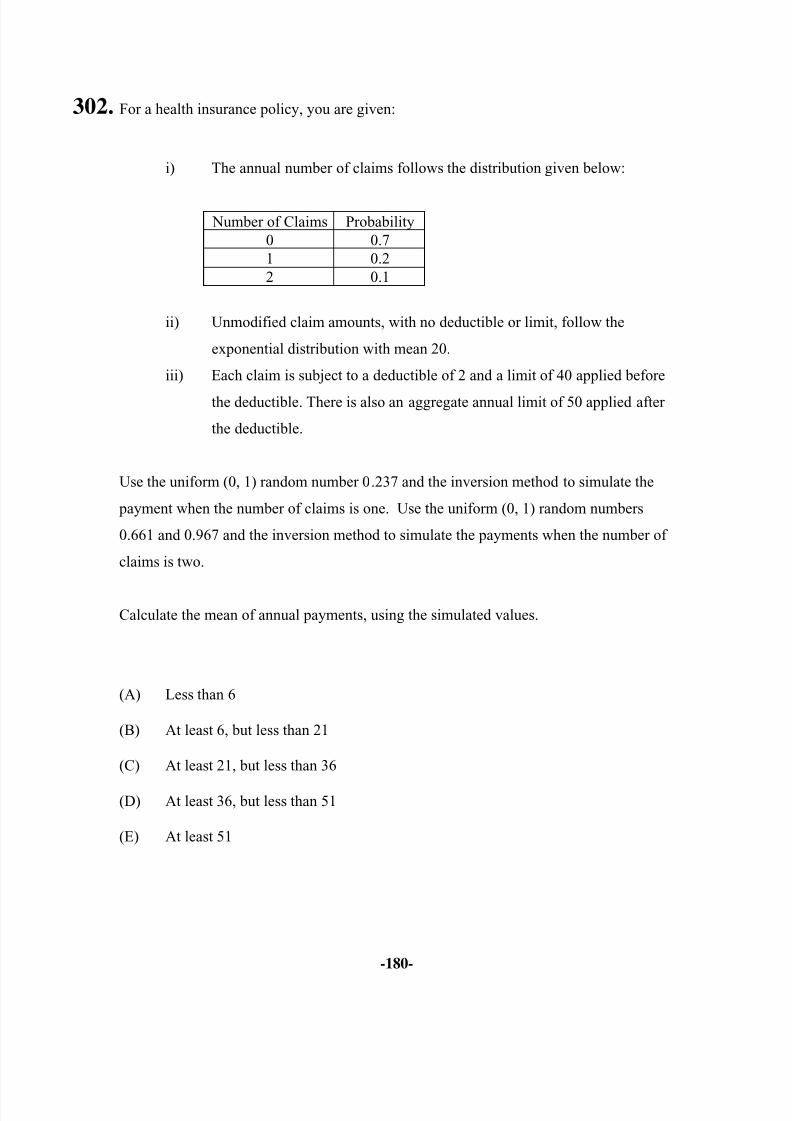
8/13/2019 Edu Exam c Sample Quest
http://slidepdf.com/reader/full/edu-exam-c-sample-quest 180/184
-180-
302. For a health insurance policy, you are given:
i) The annual number of claims follows the distribution given below:
Number of Claims Probability0 0.71 0.22 0.1
ii) Unmodified claim amounts, with no deductible or limit, follow the
exponential distribution with mean 20.
iii) Each claim is subject to a deductible of 2 and a limit of 40 applied before
the deductible. There is also an aggregate annual limit of 50 applied after
the deductible.
Use the uniform (0, 1) random number 0.237 and the inversion method to simulate the
payment when the number of claims is one. Use the uniform (0, 1) random numbers
0.661 and 0.967 and the inversion method to simulate the payments when the number of
claims is two.
Calculate the mean of annual payments, using the simulated values.
(A) Less than 6
(B) At least 6, but less than 21
(C) At least 21, but less than 36
(D) At least 36, but less than 51
(E) At least 51
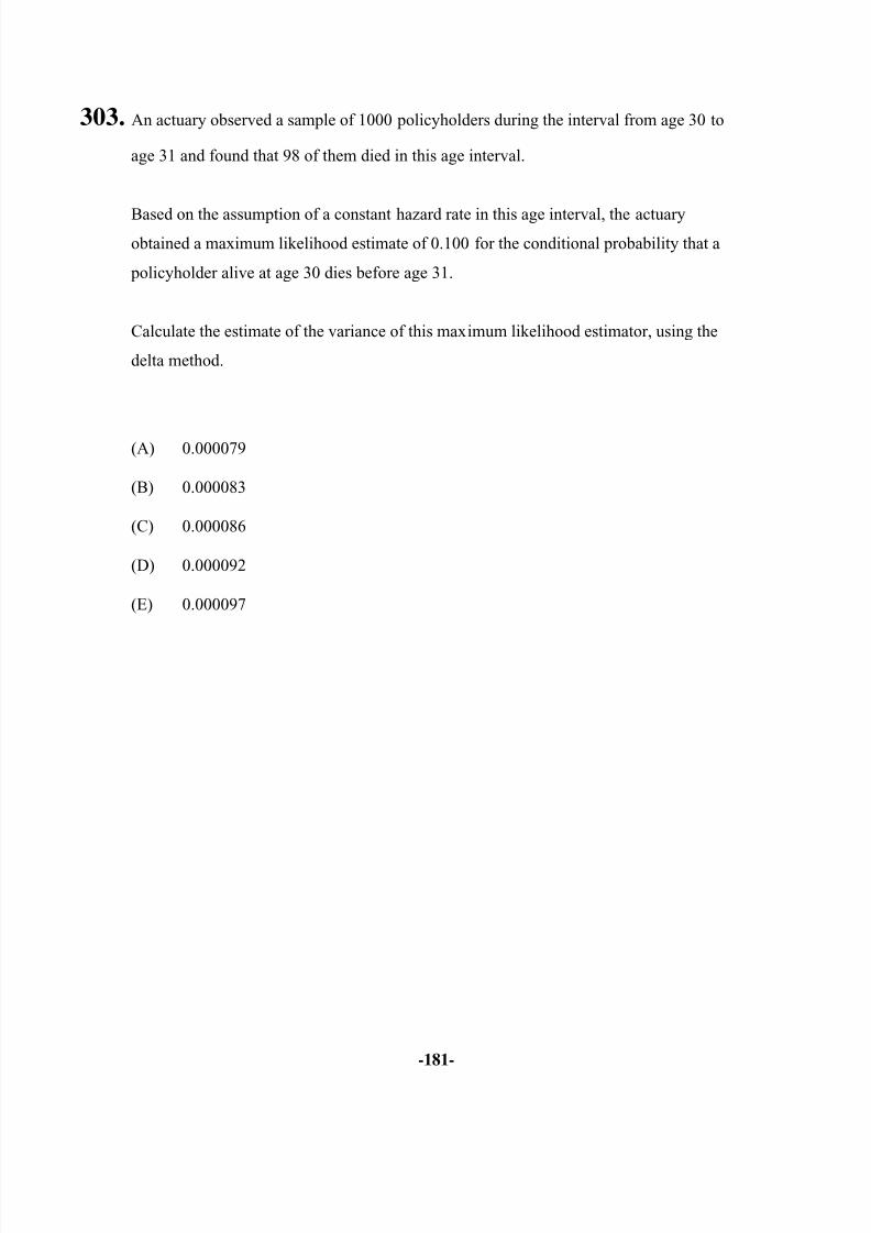
8/13/2019 Edu Exam c Sample Quest
http://slidepdf.com/reader/full/edu-exam-c-sample-quest 181/184
-181-
303. An actuary observed a sample of 1000 policyholders during the interval from age 30 to
age 31 and found that 98 of them died in this age interval.
Based on the assumption of a constant hazard rate in this age interval, the actuaryobtained a maximum likelihood estimate of 0.100 for the conditional probability that a
policyholder alive at age 30 dies before age 31.
Calculate the estimate of the variance of this maximum likelihood estimator, using the
delta method.
(A) 0.000079
(B) 0.000083
(C) 0.000086
(D) 0.000092
(E) 0.000097
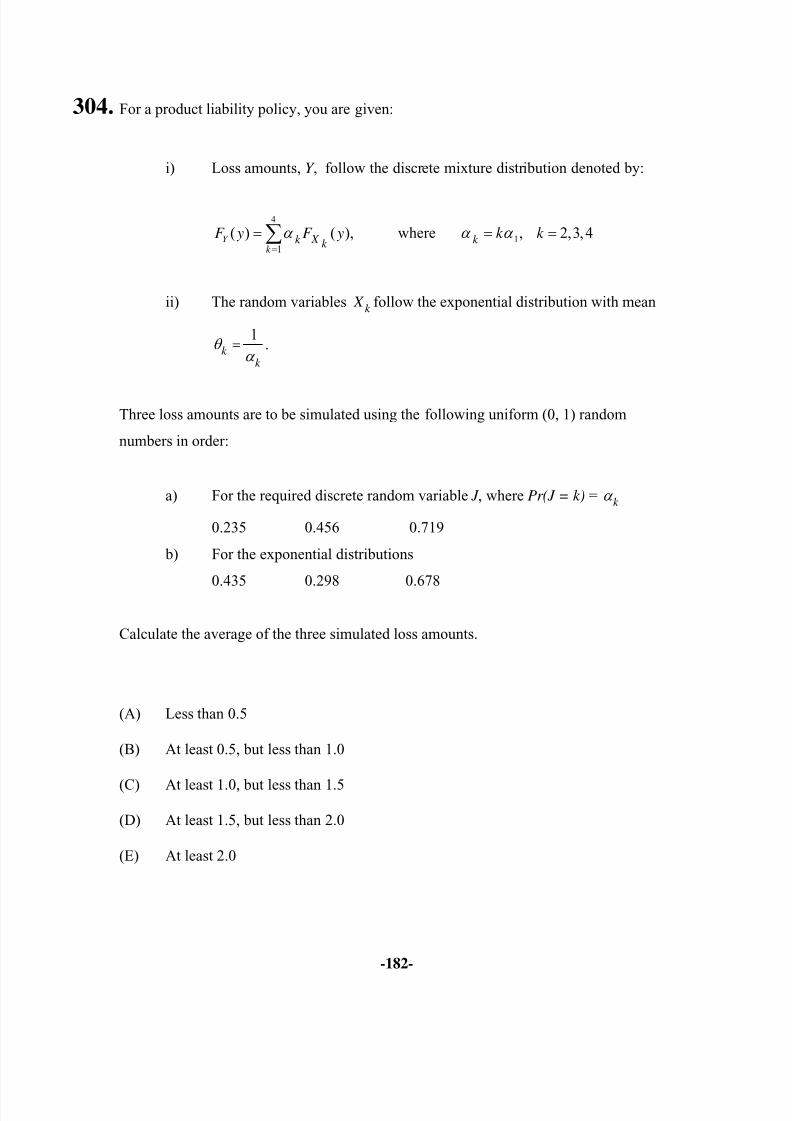
8/13/2019 Edu Exam c Sample Quest
http://slidepdf.com/reader/full/edu-exam-c-sample-quest 182/184
-182-
304. For a product liability policy, you are given:
i) Loss amounts, Y , follow the discrete mixture distribution denoted by:
4
1
( ) ( ),Y
k X k k
F y F yα =
= ∑ where 1, 2,3, 4k
k k α α = =
ii) The random variablesk
X follow the exponential distribution with mean
1.
k k
θ α
=
Three loss amounts are to be simulated using the following uniform (0, 1) random
numbers in order:
a) For the required discrete random variable J , where Pr(J = k) =k
α
0.235 0.456 0.719
b) For the exponential distributions
0.435 0.298 0.678
Calculate the average of the three simulated loss amounts.
(A) Less than 0.5
(B) At least 0.5, but less than 1.0
(C) At least 1.0, but less than 1.5
(D) At least 1.5, but less than 2.0
(E) At least 2.0
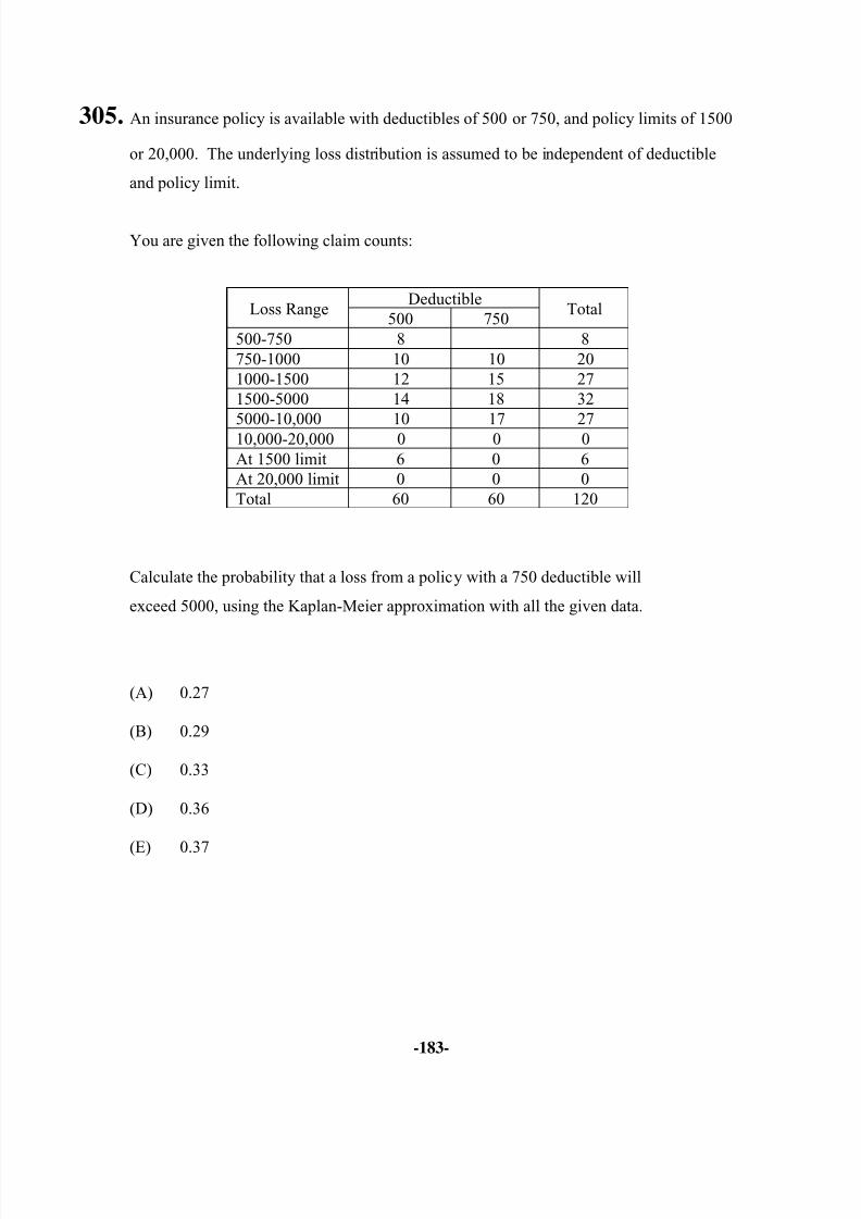
8/13/2019 Edu Exam c Sample Quest
http://slidepdf.com/reader/full/edu-exam-c-sample-quest 183/184
-183-
305. An insurance policy is available with deductibles of 500 or 750, and policy limits of 1500
or 20,000. The underlying loss distribution is assumed to be independent of deductible
and policy limit.
You are given the following claim counts:
Loss RangeDeductible
Total500 750
500-750 8 8750-1000 10 10 201000-1500 12 15 271500-5000 14 18 32
5000-10,000 10 17 2710,000-20,000 0 0 0At 1500 limit 6 0 6At 20,000 limit 0 0 0Total 60 60 120
Calculate the probability that a loss from a policy with a 750 deductible will
exceed 5000, using the Kaplan-Meier approximation with all the given data.
(A) 0.27
(B) 0.29
(C) 0.33
(D) 0.36
(E) 0.37
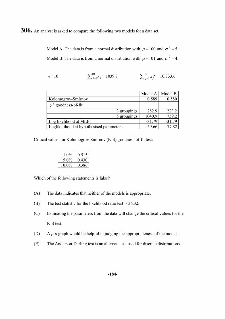
8/13/2019 Edu Exam c Sample Quest
http://slidepdf.com/reader/full/edu-exam-c-sample-quest 184/184
306. An analyst is asked to compare the following two models for a data set.
Model A: The data is from a normal distribution with 100µ = and 25.σ =
Model B: The data is from a normal distribution with 101µ = and 2 4.σ =
10n = 10
1 1039.7 j j
x=
=∑ 10 2
1 10,833.6 j j
x=
=∑
Model A Model BKolomogrov-Smirnov 0.589 0.580
2 χ goodness-of-fit
3 groupings 282.9 223.25 groupings 1040.9 739.2Log likelihood at MLE -31.79 -31.79