economics understanding world commodity prices...
TRANSCRIPT
ECONOMICS
UNDERSTANDING WORLD COMMODITY PRICES Returns, Volatility and Diversification
by
Mei-Hsiu Chen Business School
The University of Western Australia
DISCUSSION PAPER 09.03

1
UNDERSTANDING WORLD COMMODITY PRICES
Returns, Volatility and Diversification
by
Mei-Hsiu Chen1
UWA Business School
The University of Western Australia
Paper Date: August 2008
Abstract
In recent times, the prices of internationally-traded commodities have reached
record highs and there is considerable uncertainty regarding their future. This
phenomenon is partially driven by strong demand from a small number of emerging
economies, such as China and India. This paper places the recent commodity price
boom in historical context, drawing on an investigation of the long-term time-series
properties, and presents unique features for 33 individual commodity prices. Using a
new methodology for examining cross-sectional variation of commodity returns and
its components, we find strong evidence that the prices of world primary commodities
are extremely volatile. In addition, prices are roughly 30 percent more volatile under
floating than under fixed exchange rate regimes. Finally, using the capital asset
pricing model as a loose framework, we find that global macroeconomic risk
components have become relatively more important in explaining commodity price
volatility.
1 I would like to acknowledge Professor Kenneth W Clements for supervising this research and
providing helpful comments during the write-up of this paper. This paper was financially supported
by the UWA Business School and is based on my dissertation for the higher degree by research
(HDR) preliminary programme in 2007.

2
1. INTRODUCTION
Primary commodities, including raw or partially processed materials that will be
transformed into finished goods, are often the most significant source of export
earnings for many developing countries. Figure 1 shows the share of internationally-
traded non-fuel primary commodity exports in gross domestic product (GDP) for
countries around the world. A particularly striking feature in Figure 1 is the
importance of these commodities as a source of export earnings for many developing
countries. According to the United Nations Conference on Trade and Development
(1996), 57 developing countries relied on three commodities for more than half of
their total exports in 1995. For these developing countries, producing and exporting
primary commodities significantly affect their terms of trade, foreign reserve holdings,
government fiscal revenue and public expenditure. Figure 2 shows examples of
selected countries whose single most important commodity accounts for more than 50
percent of their export earnings in 1990-1999.
Figure 1
World Map – Dependence on Non-fuel Primary Commodity Exports (2006)
Source: World Bank, World Integrated Trade Solution (WITS) database. Note: The countries are colour-coded based on total exports of non-fuel primary
commodities as a percent of GDP.

3
Taking a closer look at Figure 2, we see that five countries depend on one single
commodity for more than 90 percent of their total export earnings. The highest export
concentration is Dominica, for which bananas account for a staggering 98 percent of
total export share. Export shares of many countries are highly concentrated, implying
that variation in their terms of trade correlates strongly with the price fluctuations of a
few key primary commodities. According to the World Bank’s World Development
Indicators in 1997, the ratio of primary commodities to total merchandise exports is
42 percent for developing countries. In contrast, commodity dependence is lower for
developed countries, where primary commodities accounted for only 19 percent of
their total exports in 1997.
Figure 2
Export Share of Most Important Primary Commodity for Selected Countries
0102030405060708090100K
enya
Bur
undi
Mya
nmar
Gha
na
Mau
ritan
ia
Nor
way
Chi
le
Uga
nda
Mex
ico
Icel
and
Ban
glad
esh
Mal
awi
Sri Lan
ka
Surin
ame
Cen
Afric
an R
ep
Mal
i
Ethio
pia
Nig
er
Mau
ritiu
s
Zambi
a
Dom
inic
a
Source: United Nations Commodity Trade Statistics Database (COMTRADE).
The last 20 years has predominantly been a bear market for commodities.
However by the turn of the century, the world has witnessed the biggest boom in half
a century for both fuel and non-fuel commodity prices accompanied by tremendous
Country
Tea C
off
ee
Lo
gs
Co
coa
Iro
n
Cru
de
Pet
role
um
Co
pp
er
Co
ffee
Cru
de
Pet
role
um
Fis
h
Sh
rim
p
To
bac
co
Tea Alu
min
ium
Co
tto
n
Co
tto
n
Co
ffee
Ura
niu
m
Su
gar
Co
pp
er
Ban
anas
0
10
20
30
40
50
60
70
80
90
100
Share in Total Exports (%)
Averages for 1990-99

4
price volatility. The International Monetary Fund’s non-fuel primary commodity
price index rose by 149 percent in real terms from January 2000 to June 2006, while
the energy and fuel index increased by 191 percent.2 Within the non-fuel commodity
index, the rise in the metals index is even greater at about 236 percent over the same
period. How volatile are prices for primary commodities? As an example, consider
the behaviour of the dollar price for sugar from 1948 to 2006 deflated by the United
States (US) consumer price index (CPI). The sugar price is chosen for being the most
volatile internationally tradable commodity out of 33 commodities examined in this
paper. Figure 3 shows no obvious trend in prices; however, there are several distinct
sharp peaks, particularly in the early 1960s, the late 1970s and continuing into the
early 1980s. In the 1980s, poor harvests in Cuba and the Soviet Union caused prices
to rise sharply.3 Such instances provide evidence that market abnormalities can cause
temporary surges in price volatility. Despite the volatility, the sugar price tends to
revert back to its long-run unchanging average. In other words, shocks cause the
price to deviate temporarily from this average but do not persist into the indefinite
future. That is, the mean-reverting behaviour of sugar price can be explained by the
existence of a significant temporary component in the sugar price. One salient feature
of the real sugar price that separates it from other price series is the strong appearance
of stationarity in the level; whereas typical commodity price series have tendencies of
upward or downward trends over time.
In an influential article, Deaton (1999, p. 27) notes: “What commodity prices
lack in trend, they make up for in variance.” Indeed, variability is large relative to
trend for many commodity prices. For instance, the price for sugar in 1974 was
almost three times that of the previous year and just over ten times that in 1968. The
swing from trough to peak in 1974 took only a few years. Note in Figure 3 that there
are several sharp upward spikes but no matching downward spikes, which produces
substantial positive skewness in the data. Such a characteristic is common for many
primary commodity prices.
2 According to the IMF Commodities Unit Research Department, Indices of Primary Commodity
Prices from 1995 to the present. Non-fuel primary commodities have a higher share of world export
trade (52.2 percent in 1995-1997) than energy and fuel commodities (47.8 percent). Indices of
prices are quoted in terms of nominal US dollars. To convert into real terms, nominal prices are
deflated by the US consumer price index for all urban consumers (CPI-U). Available from:
<http://www.imf.org/external/np/res/commod/index.asp> [25 April 2007]. 3 Since 1991, the Soviet Union is known as the “Union of Soviet Socialist Republics”.

5
Figure 3
Real Price for Sugar, 1948-2006
0.0
0.4
0.8
1.2
1.6
1950 1955 1960 1965 1970 1975 1980 1985 1990 1995 2000 2005
Real Price
Year
Source: Bidarkota and Crucini (2000) and the World Bank, Development Prospects Group
primary commodity price databases. Note: The underlying data are average prices for each year, deflated by the US CPI-U.
World commodity prices have risen significantly since the turn of the
millennium. However, the serious problem of volatile price uncertainty facing
commodity-dependent exporting countries has not disappeared. Previous research on
commodity returns has arrived at a remarkable degree of consensus such that real
prices have exhibited increasing variability since the breakdown of the Bretton Woods
fixed exchange rate system. It has long been noted that commodity price volatility
has exceeded that of exchange rates and interest rates. Kroner et al. (1993) show that
over the period 1972 to 1990, non-fuel commodity price volatility as measured by the
standard deviation of price changes has not been below 15 percent and peaked at more
than 50 percent per annum in 1975. In addition, short-term commodity prices can be
extremely volatile, with prices changing by as much as 50 to 100 percent in a single
year. For evidence on commodity price fluctuations see, for example, Chu and
Morrison (1984), Deaton and Laroque (1992), Yamey (1992), Reinhart and Wickham
(1994), Cuddington and Liang (1999), Deaton (1999) and Cashin and McDermott
(2002).
Today, in spite of knowledge of several stylised facts about the properties of
world commodity prices, there remain large gaps in our understanding of their
behaviour. Prior empirical work on primary commodity prices mainly focuses on the

6
question of whether the statistical evidence points to a long-term trend. Unfortunately,
not many papers have sought to investigate the global macroeconomic versus
idiosyncratic components behind commodity price variations. This paper, in contrast,
carries out an empirical study to shed light on the question of whether the price of
individual primary commodities consists mainly of global or idiosyncratic risk that
can be mitigated through proper diversification. The need to understand the
underlying risk components has taken on a new urgency in recent years as non-fuel
primary commodity prices fell sharply and persistently in real terms since 1900
although prices have risen significantly over the past few years. While this price
movement affects all commodity-exporting dependent countries to some extent, those
with the narrowly-based export bundle suffer the biggest impact. Knowledge of these
features would further our understanding of the nature of price movements in world
commodity markets that is both relevant and important for the conduct of
macroeconomic policy.
Although a substantial amount of prior research relating to risk components
focusing on the cross section of average stock returns exists, papers on distinguishing
the risk components associated with individual commodity price movements are
sparse. A notable exception is the work of Bidarkota and Crucini (2000). Based on
their empirical results of 33 primary commodities, they conclude that common and
idiosyncratic risk varies dramatically across individual commodities, and that national
terms of trade volatility could be reduced substantially by altering the export mix.
They further find that countries with high terms of trade volatility tend to have a
narrowly-based export bundle specializing in the most volatile primary commodities.
The remainder of this paper is structured as follows. Section 2 provides
theoretical background to the analysis. Annual price data and descriptive statistics on
33 commodity prices for the period 1948 through 2006 are discussed in Section 3. In
Section 4, we develop a new methodology for examining cross-sectional variations of
commodity returns and its two main components, which can be thought of as
corresponding to within-group and between-group components. The next section is
concerned with the relationship between price changes and the level of volatility of
commodity price index. Section 6 uses portfolio theory to distinguish systematic and
idiosyncratic risk factors in commodity price variations. The final section offers
caveats associated with the findings and provides a brief summary.

7
2. THEORETICAL FOUNDATIONS
Suppose that there are n commodities with price vector ( )1 2, , ..., np p p ′=p
and corresponding quantity vector ( )1 2, , ..., nq q q ′=q , so that 1
n
i iim p q
=′= =∑p q
is the total value. The value share of individual commodity i is i i iw p q m= , which
is positive and satisfies 1
1n
iiw
==∑ . Taking the differential of m and using the
identity that for any positive variable x , ( )logdx x d x= , we have
(1) ( ) ( ) ( )1 1
log log logn n
i i i i
i i
d m w d q w d p
= =
= +∑ ∑ .
Equation (1) can be written as ( ) ( ) ( )log log logd m d Q d P= + , which is a
decomposition of the change in m into indices of overall quantity change and price
change, where ( )logd Q and ( )logd P are the Divisia quantity and price indices are
defined as ( ) ( )1
log logn
i iid Q w d q
==∑ and ( ) ( )
1log log
n
i iid P w d p
==∑ ,
respectively.
If we define growth rate in the commodity price index and commodity i over the
years t-1 and t by 1log logt t tDP P P−= − and , 1log logit it i tDp p p −= − , respectively,
then these two growth rates can be linked thus
(2) 1
n
t it it
i
DP w Dp
=
=∑ ,
where itw is the arithmetic average value share of commodity i from year t to t-1 such
that ( ), 11 2it it i tw w w −= + . Equation (2) defines the index of prices as weighted first-
order moments of 1 , ..., t ntDp Dp . The corresponding second-order moment can be
expressed as
(3) ( )2
1
n
t it it t
i
w Dp DP
=
Π = −∑ .
Equation (3) is a weighted variance of the price log changes such that tΠ increases as
the individual price growth rates ( )itDp differ by more from that of the mean value
( )tDP . In other words, tΠ represents the cross-sectional standard deviation, or the
volatility of the prices.

8
Assessing the Risk: Global versus Idiosyncratic Shocks
The most common approach for measuring price volatility or risk of a primary
commodity is the coefficient of variation (CV) of the annual percent changes.
However, CV can be criticized as being a limited measure as the information it
conveys is restricted to overall volatility. On the other hand, the capital asset pricing
model (CAPM) is a useful framework for distinguishing the extent to which
commodity price volatility consists of global versus commodity-specific risk.4 The
idea behind the CAPM is that investors require compensation for the time value of
money and risk. CAPM states that the expected return of a security or a portfolio
equals the rate on a risk-free asset plus a risk premium:
(4) ( ) ( )i f i m fE r r E r rβ = + − ,
where ( )iE r is the expected rate of return on security i; fr is the rate of return of a
theoretical risk-free asset, representing the compensation required by investors for
placing money in any investment over a period of time; and iβ measures the
sensitivity of the security return to system-wide global fluctuations. Generally, a
higher iβ corresponds to higher risk, since investors are risk averse and require a
higher rate of return to compensate for holding a more risky asset. In other words, iβ
can be used as a volatility measure of the commodity relative to the market. The term
( )mE r in equation (4) is the expected rate of return of the market portfolio, such as
the Dow Jones Industrial Average or Standard & Poor’s 500 Index. Accordingly,
( )m fE r r− is the difference between the expected market return and the risk-free rate,
i.e., the risk premium, the amount of compensation that an investor needs for taking
on additional risk.
In the context of primary commodities, price variation comprises both global
risk and idiosyncratic risk. In order to decompose price movements into global and
commodity-specific risk components, the annual growth rate itDp is regressed against
some appropriate proxy for the return on a portfolio of commodity prices. For this
purpose we use, tDP , the annual growth rate of a basket of primary commodities.
That is, we estimate
4 The central foundation of the model was first formulated by Markowitz (1959) based on modern
portfolio theory, and developed a few years later by Sharp (1964), Lintner (1965) and Mossin (1966)
independently.

9
(5) it i i t itDp DPα β ε= + + ,
where iβ measures the elasticity of itp with respect to tP . The value for the
coefficient of determination for equation (5), 2R , is interpreted as the fraction of the
variation in the commodity price that is attributable to global fluctuations, as
measured by DP, while 21 R− measures the extent to which variation in prices arises
from idiosyncratic factors that are independent of global factors.
3. DATA: SOURCES, SAMPLE SELECTION AND DESCRIPTION
Most previous studies in the economics literature use the Grilli and Yang (1988)
(hereafter referred to as GY) index of real commodity prices to evaluate long-run
commodity price movements. The GY index comprises 24 primary commodity prices
running from 1900 through 1986. Unlike those studies, this paper covers a wider
range of commodities with annual price data from 1948 to 2006. As our data are
more recent, they may provide an opportunity for understanding both long-term and
recent commodity price behaviour. Our analysis considers 32 non-fuel commodities
plus crude oil that together comprise the bulk of world commodity trade. The data on
the 33 commodity prices from 1948 to 1993 are taken from Bidarkota and Crucini
(2000). We then used the World Bank Development Prospects Group’s primary
commodity price databases to supplement the Bidarkota and Crucini (2000) data,
providing a dataset from 1948 to 2006.5
The data comprise annual nominal commodity prices, and are expressed in
terms of US dollars. The real commodity price is obtained by deflating the nominal
price by the US CPI-U.6 In the subsequent analysis, no smoothing or data cleaning is
undertaken for any of the price series. This is because while smoothing may help in
the removal of outliers, it may also suppress some of the most important movements
in the commodity price data sets.
Before proceeding further, it is helpful to consider some of the salient features
of the 33 individual commodity price series. Table 1 reports the ADF results for
testing for a unit root in each of the prices. Three comments can be made about the
5 The world Bank data are from their Pink Sheet – World Bank Commodity Price Data, various issues.
The author gratefully acknowledges the help of Betty Dow in providing these data. Commodity
price data are updated monthly by the World Bank. Available from:
<http://www.worldbank.org/prospects> [13 May 2007]. 6 The US CPI-U is taken from the US Department of Labor Bureau of Statistics. Available from:
<http://www.bls.gov> [10 May 2007].

10
results. First, for 18 out of 33 prices in levels, the results in column 3 indicate the
presence of a unit root, as it fails to reject the null hypothesis of a stochastic trend at
the 5 percent significance level. Second, after applying the logarithmic
transformation, the corresponding p-values of the ADF test statistics are significant
for only 9 out of 33 cases, providing strong evidence that the null hypothesis of a unit
root cannot be rejected. Lastly, the null of a unit root is rejected for all 33
internationally-traded primary commodities when they are expressed in terms of
logarithmic first differences. In what follows, in order to induce stationarity, we use
logarithmic first differences. Log differences have the additional advantage of being
dimensionless.
Table 2 summarizes the data with commodities ranked by increasing mean price
changes. The average growth rate over nearly 60 years varies quite dramatically
across the 33 commodities and is mostly negative with the exception of seven
commodities showing a positive trend. Whilst market conditions differ across
commodities, the downward trend is quite generalized, suggesting that common
systematic factors may be responsible for the observed price declines. Commodities
whose prices have risen over the period belong to the mining and resource sectors,
except for crude oil and logs. This is inconsistent with the findings of Clements
(2004), who examined 24 commodity prices computed by GY from 1914-1986, only
five of which were demonstrated to experience price increases—none belonging to the
metals category. This discrepancy is expected due to recent strong international
demand for metals, in particular by China and other emerging markets, which have
become key drivers of price dynamics in these markets. The rise of China suggests a
fundamental change, having the effect of a long-term hardening of metals prices.
The highest annual growth rate of 127 percent was recorded in 1973-74 for
phosphate rock, the lowest being -104 percent for copra in 1974-75.7 The volatility of
7 Since any positive variable cannot fall by more than 100 percent and still stay positive, it is
important to clarify that the underlying data are annual logarithmic changes. For small changes, a
log-change, when multiplied by 100, is approximately a percentage change. The exact relationship
between the two types of changes is as follows: write 1,loglog −−= tiitit ppDp for the log-change
in the price of commodity i. Then, the corresponding percentage change is:
( )( ), 1
, 1
100100 1it
it i t Dp
i t
p pe
p
−
−
× −= × − .
Accordingly, the lowest price change is copra for which 04.1−=itDp , the implied percentage
change is ( ) 65110004.1 −=−× −
e percent.

11
Table 1
Augmented Dickey-Fuller Unit Root Tests for 33 Real Commodity Prices – Annual Observations, 1948-2006
Level Log Log First Difference
Commodity t-stat p-value lags t-stat p-value lags t-stat p-value lags
(1) (2) (3) (4) (5) (6) (7) (8) (9) (10)
1. Aluminium -4.03 0.01 * 1 -3.87 0.02* 1 -6.59 0.00 ** 0
2. Bananas -3.38 0.06 0 -4.05 0.01* 0 -7.81 0.00 ** 1
3. Bauxite -1.73 0.72 0 -1.61 0.77 0 -7.13 0.00 ** 0
4. Beef -2.13 0.52 0 -2.03 0.57 0 -7.02 0.00 ** 0
5. Cocoa -3.02 0.14 1 -1.89 0.64 2 -7.01 0.00 ** 1
6. Coconut oil -1.65 0.76 4 -2.77 0.22 2 -9.75 0.00 ** 1
7. Coffee -3.40 0.06 0 -3.11 0.11 0 -7.30 0.00 ** 0
8. Copper -2.58 0.29 0 -2.91 0.17 1 -5.69 0.00 ** 0
9. Copra -5.45 0.00 ** 1 -2.98 0.15 2 -9.49 0.00 ** 1
10. Cotton -3.37 0.07 0 -2.94 0.16 0 -7.67 0.00 ** 1
11. Crude oil -1.81 0.69 0 -1.79 0.70 0 -6.79 0.00 ** 0
12. Groundnut meal -3.96 0.02 * 0 -2.48 0.34 0 -7.51 0.00 ** 1
13. Groundnut oil -3.42 0.06 0 -3.30 0.08 0 -8.27 0.00 ** 1
14. Iron ore -2.92 0.16 1 -2.79 0.21 1 -4.90 0.00 ** 0
15. Jute -4.41 0.00 ** 1 -3.34 0.07 1 -8.36 0.00 ** 3
16. Lead -3.35 0.07 0 -2.54 0.31 0 -6.74 0.00 ** 0
17. Logs -3.18 0.10 0 -2.97 0.15 0 -7.55 0.00 ** 1
18. Maize -3.68 0.03 * 1 -3.20 0.10 0 -7.09 0.00 ** 1
19. Nickel -2.40 0.38 0 -2.58 0.29 0 -6.49 0.00 ** 1
20. Oranges -4.48 0.00 ** 0 -3.23 0.09 0 -10.22 0.00 ** 0
21. Palm oil -2.75 0.22 2 -2.07 0.55 2 -9.41 0.00 ** 1
(Table continues on the next page.)

12
Table 1 (continued)
Augmented Dickey-Fuller Unit Root Tests for 33 Real Commodity Prices – Annual Observations, 1948-2006
Level Log Log First Difference
Commodity t-stat p-value lags t-stat p-value lags t-stat p-value lags
(1) (2) (3) (4) (5) (6) (7) (8) (9) (10)
22. Phosphate rock -4.66 0.00 ** 1 -4.02 0.01* 1 -6.80 0.00 ** 1
23. Rice -4.70 0.00 ** 1 -2.46 0.34 2 -7.12 0.00 ** 1
24. Rubber -4.36 0.01 ** 0 -5.37 0.00** 1 -8.69 0.00 ** 1
25. Sorghum -3.15 0.11 1 -2.50 0.32 0 -6.59 0.00 ** 0
26. Soybean meal -4.45 0.00 ** 0 -3.22 0.09 0 -8.60 0.00 ** 1
27. Soybeans -3.64 0.03 * 0 -2.84 0.19 0 -8.40 0.00 ** 0
28. Sugar -3.90 0.02 * 0 -3.77 0.03* 1 -6.49 0.00 ** 0
29. Tea -3.97 0.02 * 0 -3.80 0.02* 0 -8.18 0.00 ** 0
30. Tin -1.64 0.76 0 -1.64 0.76 0 -7.04 0.00 ** 0
31. Tobacco -3.04 0.13 0 -4.15 0.01** 2 -7.58 0.00 ** 0
32. Wheat -4.61 0.00 ** 1 -4.00 0.01* 1 -6.75 0.00 ** 1
33. Zinc -3.92 0.02 * 1 -3.69 0.03* 1 -5.44 0.00 ** 0
Notes: 1. The regression is 1 1 1t t i t i tiy t y yα β ρ ρ ε− −≠
= + + + +∑ for real commodity prices in levels, logarithms and first
differences of the logarithms, with an automatic lag length selection using a Schwarz Information Criterion and
maximum lag length set equal to 10.
2. Double and single asterisks (** and *) denotes the p-value significant at the 1% and 5% levels, respectively.

13
this annual growth rate is remarkable—the standard deviation of the price changes
ranges from 10 percent for tobacco, to as high as 39 percent for sugar (see column 6).
Despite ranking lowest in the price fluctuation ladder, the price movement for tobacco
is nowhere close to being stable. The average volatility of the annual change in
logarithm returns for the 33 commodity prices over the period 1948 to 2006 is more
than 21 percent (last row of column 6). Clearly, on a year-to-year basis, commodity
prices are highly volatile—and this volatility would be even higher if monthly or daily
data were used, as the use of annual rather than monthly data has the effect of
smoothing out many of the short-term fluctuations. Some commodities are associated
with annual percent changes well over 100 percent (columns 7 and 8), which is
obviously huge. Table 2 demonstrates a relatively large dispersion in price changes
(column 6) that dominates small secular changes (column 2) for all cases. In other
words, the long-term trend for each individual commodity appears to be widely
variable, reflecting the large uncertainties associated with these commodities.
In constructing an index of commodity prices, one importance issue to consider
is whether equal weighting, instead of a consumption/production weighting system,
introduces substantial bias. To investigate this issue, Figure 4 sets out both the
weighted GY commodity price index (“GYCPI”), together with an equally-weighted
index of this study over the period 1948 to 2003. Both indices are expressed in terms
of levels with a common base year for easy comparison. An interesting feature about
Figure 4 is the high degree of correlation between the two indices; the correlation is
0.995 over 1948 to 1986 (denoted by unshaded region), and increases slightly to 0.996
when the GYCPI is extended to 2003 (denoted by shaded region) by Pfaffenzeller et
al. (2007) (both p-values < 0.01). This finding is remarkable since there are
qualitative differences in the values of the two price indices, one uses 24 export-
weighted commodities and the other 33 equally-weighted primary commodities.
Given the high correlation between the two series, the equally-weighted price index
employed in this paper seems to support the notion that the trends in broad indices of
the prices of primary commodities are not much affected by the different weighting
systems used to compute them.

14
Table 2
Summary Statistics – Logarithmic Changes in Real Prices of 33 Commodities
Annual Observations, 1948-2006 Standard Deviation
Commodity Mean Median 1948-71 1972-06 1948-06
Minimum Maximum Jarque-Bera p-value
(1) (2) (3) (4) (5) (6) (7) (8) (9) (10)
1. Jute -3.85 -2.68 28.16 22.66 24.84 -86.00 52.10 17.10 0.00 **
2. Groundnut meal -3.54 -2.80 9.61 26.03 20.06 -65.86 71.91 38.57 0.00 **
3. Palm oil -3.33 -1.00 13.78 28.06 23.31 -68.59 49.19 0.71 0.70
4. Copra -3.28 0.47 19.59 39.62 32.95 -103.63 85.74 2.64 0.27
5. Coconut oil -3.14 0.63 16.48 39.52 32.20 -101.80 72.46 4.20 0.12
6. Tea -3.05 -4.64 12.32 18.65 16.31 -59.11 49.61 24.06 0.00 **
7. Cotton -2.94 -3.93 12.73 20.67 17.82 -40.22 47.54 4.55 0.10
8. Rice -2.83 -2.93 11.88 23.85 19.86 -55.97 69.68 20.57 0.00 **
9. Tobacco -2.55 -3.03 11.27 9.57 10.25 -27.33 20.25 0.83 0.66
10. Soybean meal -2.47 -2.42 15.63 23.94 20.89 -60.02 79.03 33.32 0.00 **
11. Cocoa -2.39 -3.94 28.02 24.68 25.84 -57.26 55.40 1.85 0.40
12. Soybeans -2.35 -3.84 16.44 18.07 17.30 -46.23 66.79 40.00 0.00 **
13. Groundnut oil -2.29 -5.33 13.97 26.11 21.96 -63.80 57.46 3.11 0.21
14. Wheat -2.24 -2.00 6.50 18.84 15.16 -31.58 66.46 103.43 0.00 **
15. Sorghum -2.16 -2.18 8.97 16.18 13.68 -33.65 44.69 6.70 0.04 *
16. Maize -1.84 -3.92 12.12 17.73 15.65 -37.06 49.93 14.80 0.00 **
17. Oranges -1.80 -4.62 15.68 13.62 14.56 -37.88 46.63 5.65 0.06
18. Lead -1.55 -0.13 20.54 25.19 23.36 -43.95 51.68 0.88 0.64
19. Sugar -1.51 -0.33 37.50 40.00 38.69 -103.59 103.47 5.70 0.06
(Table continues on the next page.)

15
Table 2 (continued)
Summary Statistics – Logarithmic Changes in Real Prices of 33 Commodities
Annual Observations, 1948-2006 Standard Deviation
Commodity Mean Median 1948-71 1972-06 1948-06
Minimum Maximum Jarque-Bera p-value
(1) (2) (3) (4) (5) (6) (7) (8) (9) (10)
20. Tin -1.26 -1.02 12.85 21.64 18.55 -64.58 52.71 13.32 0.00 **
21. Phosphate rock -1.10 -2.37 9.05 26.87 21.51 -67.72 126.88 1,180.63 0.00 **
22. Coffee -1.06 -3.96 17.48 29.91 25.55 -57.45 72.62 6.89 0.03 *
23. Rubber -0.97 -3.75 29.88 21.84 25.14 -47.82 84.32 11.03 0.00 **
24. Bananas -0.93 -0.85 8.28 13.92 11.96 -36.64 31.00 6.08 0.05 *
25. Bauxite -0.60 -1.93 9.89 13.61 11.77 -16.90 51.37 289.20 0.00 **
26. Beef -0.16 -0.13 8.52 13.82 12.35 -34.46 27.72 0.60 0.74
27. Aluminium 0.02 0.60 4.33 18.87 14.82 -31.52 44.81 2.92 0.23
28. Zinc 0.36 0.63 21.57 28.03 25.56 -69.58 83.16 16.24 0.00 **
29. Iron ore 0.51 -1.61 11.27 13.15 12.36 -16.81 50.61 41.47 0.00 **
30. Logs 0.57 -0.22 14.42 22.74 19.72 -39.86 59.14 5.57 0.06
31. Copper 0.71 -0.82 20.20 24.24 22.54 -59.69 57.10 0.29 0.87
32. Crude oil 2.08 -4.26 9.13 32.70 26.30 -65.71 125.82 196.73 0.00 **
33. Nickel 2.21 1.84 5.15 28.16 22.00 -45.90 99.90 92.66 0.00 ** All commodities -1.47 -1.90 16.45 24.13 21.38 -103.63 126.88
Sources: The 33 commodity annual time series data are taken from Bidarkota and Crucini (2000) and the World Bank, Development Prospects Group
primary commodity price databases.
Notes: The underlying data are calculated as nominal commodity prices deflated by the US CPI-U over the period 1948 to 2006. Entries in columns 2 to
8 are to be divided by 100. The Jarque-Bera statistic tests the null hypothesis that the distribution conforms to a Gaussian normal distribution.
Significance at the 1% and 5% confidence levels is indicated by ** and *, respectively.

16
Figure 4
Index of Nominal Non-Fuel Commodity Prices – Annual Observations (1948-2003)
20
40
60
80
100
120
140
1950 1955 1960 1965 1970 1975 1980 1985 1990 1995 2000
Sources: 1. GYCPI (unshaded region): Grilli and Yang (1988).
2. Extension of GYCPI (shaded region): Pfaffenzeller et al. (2007).
3. CI: Annual time series data are taken from Bidarkota and Crucini (2000) and the
World Bank, Development Prospects Group primary commodity price database.
Note: GYCPI and extension of GYCPI are based on 24 internationally-traded non-fuel
primary commodities, whereas CI is based on 32 non-fuel commodities. All
price series are indexed to their 1977-1979 average.
4. VOLATILITY OF COMMODITY PRICES
A striking feature of the behaviour of primary commodities after the collapse of
the Bretton Woods fixed exchange rate system has been the high level of price
volatility, though this does not imply volatility was particularly low prior to 1971.
Results in columns 4 and 5 of Table 2 reveal that commodity price volatility on
average has been higher in the post-1971 period than in the previous 20 years for all
except 5 commodities. Overall, price volatility averages about 21 percent from 1948
to 2006. This section sheds light on the nature and sources of this volatility.
A Group-Wise Decomposition
Suppose we group the n commodities into G categories, denoted by
1 2, , ..., GS S S , where G < n. Each commodity i belongs to one category only, so
generally one can write gi S∈ , and g = 1, …, G. As nwit 1= is the weight of
commodity i with 1
1n
itiw
==∑ , one can define nnwW g
gSi itgt ==∑ ∈ as the
weight for group g, with 1
1G
gtgW
==∑ , where
gn is the number of goods in group g.
GYCPI
CI (this study)
Year
Extension
Index (1977-79 = 100)
17
Let the share of gi S∈ within its group be 1it it gt gw w W n′ = = , which satisfies
1g
iti Sw
∈′ =∑ . Then gtDP , the logarithmic annual return for group g at time t, can be
written as
(6)
g
gt it it
i S
DP w Dp
∈
′= ∑ .
Given that the overall, or composite, price index was defined earlier as
1
n
t it itiDP w Dp
==∑ , it can be written in terms of gtDP as
(7) 1
G
t gt gt
g
DP W DP
=
=∑ ,
A comparison of equations (6) and (7) with equation (2) reveals that the model is
consistent in aggregation. To clarify this, consider two ways to compute the overall
price index tDP :
A. Use the prices to compute the G group indices, gtDP , g = 1, …, G,
according to equation (6) and then take the weighted average of these to
gives the overall index tDP according to equation (7).
B. Compute tDP directly from equation (2).
Consistency in aggregation means that these two approaches give exactly the same
result for tDP .
We shall use G = 3 groups, food, non-food agricultural and metals commodities.
The commodities in each sub-index are given in Table A1.1 of Appendix A1. Note
that since crude oil does not belong to any of the sub-groups, in what follows, we use
n = 32 rather than 33. Rows 1 to 7 of Table 3 show the decomposition of the total
index by decades and rows 8 to 9 break the sample period on the basis of exchange
rate regimes. Metals is the only group experiencing positive average growth in real
prices over the past 58 years. This positive growth is primarily attributed to the strong
price increases over the period 2001-2006, when prices grew by more than 10 percent
per annum. In contrast, the recent upturns in food and non-food prices have been
comparatively small at about one-third of the growth of metals. Table 3 shows that
food prices declined in all periods except for 1971-1980 and 2001-2006. Although
annual growth rate is positive during these two periods, it is either significantly lower
than or approximately the same as the average growth rate tDP . The growth rate of

18
non-food prices is bounded by that of metals from above, and of food from below.
The recent upturn in commodity prices has been large and rapid and is rivalled by
only one other period over the last 58 years which is the commodity price boom of the
1970s. Over these two periods, prices for all three groups show a persistent upward
trend.
Table 3
Average Annual Growth Rate for Commodity Sub-Categories, 1948-2006
Sub-Indices
Food Non-Food Metals Total
Period 1tDP 2tDP 3tDP tDP
(1) (2) (3) (4) (5)
1. 1948-1950 -2.66 4.27 1.77 -0.33
2. 1951-1960 -3.24 -1.26 -0.88 -2.27
3. 1961-1970 -1.07 -4.81 0.22 -1.29
4. 1971-1980 1.96 2.38 2.76 2.25
5. 1981-1990 -7.56 -4.61 -4.29 -6.18
6. 1991-2000 -4.47 -4.73 -4.38 -4.52
7. 2001-2006 3.36 2.03 10.78 5.15
8. 1948-1971 -2.42 -2.42 -0.48 -1.87
9. 1972-2006 -2.10 -1.54 0.39 -1.34
10. 1948-2006 -2.22 -1.89 0.04 -1.55 Note: All entries are to be divided by 100 and are simple averages over the
corresponding periods.
Equation (6) is a weighted first-order moment of 1 , ..., gt n tDp Dp . The
corresponding second-order moment is
(8) ( )2
g
gt it it gt
i S
w Dp DP
∈
′Π = −∑ ,
which measures the dispersion across commodities within the group. Table 4 gives
gtΠ for the period 1948 to 2006. Over the fixed exchange rate regime, prices of
metals tended to be reasonably tranquil with a standard deviation of 0137.03 =Π ,
or about 12 percent. In contrast, metals price volatility increased substantially after
the collapse of the Bretton Woods fixed exchange rate system. On average, the
volatility of food prices also increased substantially from the fixed to managed-

19
floating exchange rate systems, but non-food remained fairly stable. This finding is
consistent with earlier work by Deaton and Laroque (1992) and agrees with previous
research indicating exchange-rate movements as a major cause of commodity price
instability (see, for example, Sjaastad and Scacciavillani 1996). Finally, the last row
of Table 4 shows that on average over the whole period, there is greater price
dispersion for food as a group, followed by non-food and metals. Overall, Table 4
shows that price volatility appears to be persistent over time.
One other feature of Table 4 is worthy of note. Column 5 gives the weighted
average of the within-group variances. Interestingly, this value is always lower but
close to the total variance shown in the last column. Looking at the last entries of the
last two columns of the table, the differences is on average 13.346.3 − = 33 basis
point. What is the reason for this discrepancy between the two values? The answer is
provided in the next sub-section.
Table 4
Average Price Variability for Commodities, 1948-2006
Sub-Indices
Food Non-Food Metals
Weighted
average Total
Period t1Π t2Π t3Π gtg gtW Π∑ =
3
1 tΠ
(1) (2) (3) (4) (5) (6)
1. 1948-1950 5.84 7.74 0.72 4.70 5.18
2. 1951-1960 1.75 3.64 1.67 2.02 2.44
3. 1961-1970 2.58 1.24 1.22 1.99 2.13
4. 1971-1980 6.98 2.68 4.58 5.63 5.94
5. 1981-1990 4.07 2.81 3.15 3.61 3.93
6. 1991-2000 2.78 2.80 1.44 2.42 2.68
7. 2001-2006 2.83 1.53 2.76 2.61 3.18
8. 1948-1971 2.44 2.84 1.37 2.20 2.49
9. 1972-2006 4.40 2.60 3.06 3.75 4.10
10. 1948-2006 3.62 2.69 2.39 3.13 3.46
Notes: 1. All entries are to be divided by 100 and are simple averages over the
corresponding periods.
2. The total variance tΠ shown in the last column is defined as
( )32 2
1 it it tiw Dp DP
=−∑ .

20
Within- and Between-Group Volatility
As demonstrated earlier, the cross-sectional standard deviation of world
commodity prices at time t is given by equation (3), ( )2
1
n
t it it tiw Dp DP
=Π = −∑ . In
the context of commodity sub-groups, some of the cross-sectional price dispersion are
potentially the consequence of within-group variations while the remaining variations
can be attributed to between-group components. This sub-section analyses the
importance of each component by means of a simple decomposition.8 Consider the
identity ( ) ( ) ( )2
2 2
1 11 1
n n
i ii in x x n x x
= =− = −∑ ∑ . One can then use a weighted
version of this identity to express the cross-sectional price variance of equation (3) as
(3′) 2 2
1
n
t it it tiw Dp DP
=Π = −∑ ,
while the cross-sectional variance of group g, equation (8), is
2 2
ggt it it gti S
w Dp DP∈
′Π = −∑ . Take the weighted average of the G group variances to
obtain
2 2 2 2
1 1 1 1g
G G n G
gt gt gt it it gt it it gt gt
g g i S i g
W W w Dp DP w Dp W DP
= = ∈ = =
′Π = − = −
∑ ∑ ∑ ∑ ∑ .
Rearrange and bring the term 2
1
n
it itiw Dp
=∑ to the left-hand side so that
(9) 2 2
1 1 1
n G G
it it gt gt gt gt
i g g
w Dp W W DP
= = =
= Π +∑ ∑ ∑ .
Substituting equation (9) into equation (3′), the variance for n commodities can be
written as the sum of the weighted average of the variances for the G sub-groups and
the variance between the sub-groups:
(10) ( )2
1 1
G G
t gt gt gt gt t
g g
W W DP DP
= =
Π = Π + −∑ ∑ .
Equation (10) provides a simple and elegant decomposition. The total price volatility
can be decomposed into two components: The first term is a weighted average of
1 , ..., t GtΠ Π , the variances of the G groups, corresponding to a “within-group”
8 The decomposition analysis used in this paper is based on that of Chan and Clements (2007). They
investigate the cross-country distribution of the world economic growth, and the components of
growth volatility.

21
component. The second term, ( )2
1
G
gt gt tgW DP DP
=−∑ , is a “between-group”
component. This thus provides the answer to the question raised at the end of the
previous sub-section regarding the discrepancy between the total variance and the
weighted average of the variances over the G sub-groups. Since the difference
between the two values is small in Table 4, we see that the between-group component
is not a dominant factor affecting the overall variance. In other words, within each
commodity group on average, there is more price volatility relative to that between
groups. The above also shows that tΠ always exceeds 1
G
gt gtgW
=Π∑ since the
between-group component is always a positive value. This can be confirmed by a
comparison of columns 5 and 6 of Table 4.
Table 5 demonstrates that the total price variance can be decomposed into
within- and between-group components, and that the discrepancy observed earlier in
Table 4 can be explained by the between-group component, given in columns 6 to 9
of Table 5. The within-group component (column 5) first decreases over time until
the breakdown of the Bretton Woods fixed exchange rate system. This is where the
within-group component rises almost three-fold compared to the previous decade and
reaches a record high with average annual growth of 5.63 percent, but thereafter
decreases substantially. The between-group component shows a similar pattern over
time except that the highest price variation is recorded after the turn of the century.
This finding supports the view that relative prices of primary commodities exhibit
greater volatility under flexible relative to fixed exchange rate regimes. On average,
real price variability under the floating exchange period is roughly 30 percent larger
than under the fixed exchange period (that is, 4.10 2.49 1.3≈ ). The volatility of
commodity price returns, tΠ , is 15.8 percent over the pre-1972 period, and grew
substantially higher post-1972 to 20.2 percent per year.
Interestingly, in the within-group components, food (column 2) is the dominant
source of dispersion. Such a result may not come as a surprise since the commodities
in this group alone account for nearly 60 percent of the share of the overall price
index. In addition, the effect of the between-group component is significantly smaller
than its within-group counterparts in overall price volatility. In all cases, the between-
group component accounts for less than 20 percent of price variability, whereas the
within-group component accounts for the remaining 80 percent.

22
Table 5
Decomposition of Price Volatility into Within- and Between-Group Components, 1948-2006
Within-Group Components Between-Group Components
Food Non-Food Metals Sum Food Non-Food Metals Sum
Total
Variance
Period 1 1W Π 2 2W Π 3 3W Π
3
1
g g
g
W
=
Π∑
( )2
1 1W DP DP− ( )22 2W DP DP− ( )2
3 3W DP DP− ( )3 2
1
g g
g
W DP DP=
−∑ tΠ (1) (2) (3) (4) (5) (6) (7) (8) (9) (10) = (5) + (9)
1. 1948-1950 3.28 1.21 0.20 4.70 0.11 0.07 0.30 0.48 5.18
2. 1951-1960 0.98 0.57 0.47 2.02 0.09 0.17 0.16 0.42 2.44
3. 1961-1970 1.45 0.19 0.34 1.99 0.04 0.05 0.06 0.15 2.13
4. 1971-1980 3.92 0.42 1.29 5.63 0.08 0.08 0.15 0.31 5.94
5. 1981-1990
2.29 0.44 0.89 3.61 0.07 0.14 0.10 0.32 3.93
6. 1991-2000 1.59 0.44 0.39 2.42 0.08 0.05 0.14 0.27 2.68
7. 2001-2006 1.62 0.25 0.75 2.61 0.15 0.04 0.38 0.57 3.18
8. 1948-1971 1.37 0.44 0.38 2.20 0.07 0.10 0.12 0.29 2.49
9. 1972-2006 2.49 0.41 0.85 3.75 0.09 0.08 0.18 0.35 4.10
10 1948-2006 2.04 0.42 0.67 3.13 0.08 0.09 0.15 0.33 3.46 Note: All entries are to be divided by 100 and are simple averages over the corresponding periods.

23
More Decompositions – A CAPM Approach
Consider the change in the price of commodity i relative to the mean,
it tDp DP− . It is natural to consider the weighted deviation ( )titit DPDpw − , which
satisfies ( ) 0it it tiw Dp DP− =∑ . Suppose this weighted deviation is a linear function
of the price index, tDP :
(11) ( )it it t i i t itw Dp DP DPα β ε′ ′ ′− = + + ,
where iα ′ is the intercept, iβ ′ is the slope coefficient and itε ′ is the error term
reflecting omitted factors. As ( )1
0n
it it tiw Dp DP
=− =∑ , each term on the right-hand
side of equation (11) has a zero sum over the n commodities, which implies
(12) 1 1 1
0n n n
i i it
i i i
α β ε= = =
′ ′ ′= = =∑ ∑ ∑ .
Now assume individual commodities are grouped into their respective
categories: food, non-food and metals. Then if we add the left-hand side of equation
(11) over gi S∈ we obtain
( ) ( )g g g
it it t it it it t gt gt t
i S i S i S
w Dp DP w Dp w DP W DP DP
∈ ∈ ∈
− = − = −∑ ∑ ∑ ,
where ∑ ∈=
gSi itgt wW is the share for group g, as before. Similarly, the right-hand
side of equation (11) can be aggregated as
g g gi i it g g t gti S i S i S
DP A B DP Eα β ε∈ ∈ ∈
′ ′ ′+ + = + +∑ ∑ ∑ , where g
g ii SA α
∈′=∑ ,
gg ii S
B β∈
′=∑ , and g
gt iti SE ε
∈′=∑ . Therefore, the group-wise version of equation
(11) for group g takes on the form
(11′) ( ) gttggtgtgt EDPBADPDPW ++=− .
Comparing equation (11) with (11′), we see that the latter is just an
“uppercase” version of the former, so that the model is consistent in aggregation. As
shown from equation (7), tDP is the weighted average of all gtDP , indicating that the
summation of the weighted deviation of growth in group g from the average growth
rate is zero, such that ( ) 01
=−∑ =G
g tgtgt DPDPW . As the left-hand side of equation

24
(11′) when summed over the g sub-groups is zero, it follows that the right-hand side
of equation (11′) satisfies
(13) 0
111
∑∑∑===
===G
g
gt
G
g
g
G
g
g EBA .
To interpret equation (11′), divide by gtW and add tDP to the both sides, to obtain
the growth of group g as
(14) gt
gtt
gt
g
gt
ggt
W
EDP
W
B
W
ADP +
++= 1 .
Equation (14) is exactly the same as the CAPM equation mentioned earlier in Section
3 but now refers to groups of commodities rather than individual commodities.
Therefore, the first term on the right of equation (14) is the intercept that captures the
influence of idiosyncratic factors independent of common factors unique to each
group g. The second term is the slope coefficient, representing the return to group g
that is attributed by the systematic factors common to all commodity groups. Finally,
the last term, gtgt WE , denotes the remaining risk factors not captured by systematic
or idiosyncratic risk. The term ( )gtg WB+1 also measures the elasticity of gtP with
respect to tP . In other words, if the growth rate of the prices of group g coincides
with mean growth rate tDP , the elasticity is unity, so that gtg WB , or simply gB , is
zero. The term gtg WB is the beta coefficient for group g. The coefficient, gB , can
be positive or negative depending on whether group g grows faster or slower relative
to the mean growth rate.
Table 6 presents the OLS estimates of equation (11′) for G = 3 sub-indices
over the period 1948 to 2006. The intercept gA represents the impact of overall
growth for each group g attributed by idiosyncratic risk factors and is found to be
insignificantly different from zero for all three sub-groups. This result is consistent
with the portfolio theory: when combining an individual commodity into its respective
category, such diversity helps to eliminate the effects of highly idiosyncratic events
which are likely to have large implications for the individual commodity markets. In
other words, when aggregated into sub-indices, the overall risk is reduced without
sacrificing any returns. In such cases, systematic economic forces have become the

25
major source of price instability influencing the world commodity markets. The
elasticity of growth (column 7) for the food subgroup is 1.04—only slightly higher
than its metals counterpart, which has an elasticity of 1.02. Hypothesis testing reveals
that both elasticities are statistically insignificantly different from unity (see columns
4 and 5). On the other hand, the non-food elasticity of growth is shown to be
substantially lower than those of the food and metals sub-groups, being equal to 0.82
over the sample period.
Table 6
Price Growth Decomposition into Systematic and Idiosyncratic Risk, 1948-2006
Intercept gA Slope gB
Sub-Index Coefficient SE Coefficient SE g gtA W
Elasticity
1 g gtB W+
(1) (2) (3) (4) (5) (6) (7)
1. Food -0.29 0.32 0.02 0.03 -0.51 1.04
2. Non-food -0.11 0.18 -0.03 0.02 -0.69 0.82
3. Metals 0.40 0.30 0.01 0.03 1.41 1.02 Sum 0.00 0.00
Note: SE denotes standard error.
5. ON THE RELATION BETWEEN PRICES AND VOLATILITY
The proposition that the average rate of change of prices has an effect on the
variability of relative price changes has given rise to an extensive empirical literature.
Vining and Elwertowski (1976) conclude that there is a positive relationship between
the variance of relative prices and the general price change, although the authors fail
to provide any explanations of their result. In contrast, Parks’ (1978) seminar paper
considers a multimarket model of prices that he applies to the US over the periods
1930-1941 and 1948-1975. His results show a significant association between the
variance of relative prices and the rate of inflation. However, it must be emphasised
that Parks’ findings are controversial as several authors subsequently argued that the
relationship between price variability and inflation is only a by-product of the oil
shock in 1974.9 This section considers if the variability of commodity prices is
related to their overall average change.
9 See, for example, Bomberger and Makinen (1993) and Jaramillo (1999).

26
There can be little doubt that the collapse of Bretton Woods fixed exchange rate
system has contributed substantially to the variability of the prices of internationally-
traded primary commodities. Panel A of Figure 5 shows the plot of annual volatility
of 33 commodity price series, tΠ , against time. Interestingly, price volatility has a
tendency to revert back to the mean over time. This finding is consistent with
Pindyck (2001) who examines price volatility at the individual commodity level. By
using daily and weekly data for the three commodities that make up the petroleum
complex, he finds rapid mean reverting of price volatilities for crude oil, heating oil
and gasoline over the period 1984 to 2001.
Figure 5
Annual Volatility and Composite Price Index, 33 Commodity Prices, 1948-2006
0
20
40
60
1950 1955 1960 1965 1970 1975 1980 1985 1990 1995 2000 2005
0
40
80
120
160
1950 1955 1960 1965 1970 1975 1980 1985 1990 1995 2000 2005
(% p.a.)
tΠ
Year
Year
Index (1977-79 = 100)
B. Real Price Index Series
A. Cross-Sectional Volatility
Notes: 1. Volatility is based on cross-sectional standard deviation of 33 commodity price series.
2. Real price is obtained by deflating nominal price by US CPI-U.

27
There is evidence of lower price volatility prior to the 1970s. Generally,
volatility fluctuates up and down quite sporadically and there appears to be a sudden
rise in 1974. What has caused this jump in volatility? Panel B above shows real price
index for 33 commodities, which provide some indications about the rapid change in
volatility level shown in Panel A. The sharp rise in the price index following the
effects of the Arab oil embargo in 1973 seems to be the cause of the spike in volatility.
As illustrated by the gray dotted line, the peak in the level of volatility coincides well
with the peak in the overall price index. Furthermore, the spikes observed in Panel A
in year 1951 and 1986 seem to perfectly match either a peak or trough in the
corresponding price index in Panel B. This thus provides some preliminary evidence
regarding to interrelationship between volatility and the level of commodity prices.
Figure 6 shows the plot of annual volatility together with the log-changes of the
price index (fuel included) from 1948 to 2006. It can be seen that when volatility is
relatively low over the period 1954 to 1972, the price index is mostly below its 58-
year average and corresponds to modest price changes that tend to fall in the band ±10
percent. Throughout the remaining period where the rates of change in volatility are
much higher, the index of price changes itself tends to be more volatile.
Figure 6
Relationship between Volatility and Relative Change in Price Index, 1948-2006
-20
0
20
40
1950 1955 1960 1965 1970 1975 1980 1985 1990 1995 2000 2005
Next, Figure 7 provides the same information in the form of a scatter plot of
volatility against the absolute value of tDP . Only four out of the 58 points lie below
the 45-degree line, suggesting that volatility is higher than average price changes.
Year
Price index: annual log-changes,
Annual volatility,
mean = 17.9%
mean = -1.4%
(% p.a.)
tΠ
tDP

28
This observed difference between the behaviour of commodity price variance and
change in relative prices was noted previously (see, for example, Cashin and
McDermott 2002; Deaton 1999). The four points that lie below the 45-degree line
correspond to 1973, 1981, 1982 and 1985. In 1973 there is a positive price change of
35 percent. In contrast, world commodities experienced a fall in prices for the other
three years, -17 percent in 1981, -21 percent in 1982 and -19 percent in 1985. The
most important question is: does the conclusion drawn by Parks (1978) regarding to
the relationship between inflation rate and variance of relative prices changes still
survive? Figure 7 indicates a positive relationship between the two variables with a
correlation coefficient of 0.55; this decreases slightly to 0.49 when the 1974
observation is excluded. Both these estimates are statistically significant at the 1
percent level.
A summary of this material is as follows. There is a strong and positive
relationship between the variance of relative price changes and the average rate of
price changes. In addition, this relationship remains strong even after removing data
from 1974, when the price of oil suffered severe shocks. Such results are inconsistent
with the evidence from previous studies.
Figure 7
Scatter Plot of Volatility Against Absolute Log-Changes in Relative Price Index,
1948-2006
0
5
10
15
20
25
30
35
40
45
0 5 10 15 20 25 30 35 40
correlation = 0.55
t-statistic = 4.91
45°
tΠ
1973
1981
1982
1985
(% p.a.)
(% p.a.) tDP
1974

29
6. GLOBAL VERSUS IDIOSYNCRATIC RISK
This section splits fluctuations in commodity prices into global and
idiosyncratic parts. Variations in commodity returns may be the result of common
movements in macroeconomic variables that affect the demand for or the supply of
broad sets of commodities, as well as commodity-specific factors that are unique to
each commodity. Conceptually, the former component cannot be diversified away by
combining with other commodities in a portfolio, whereas the latter can. A better
understanding of these two components provides some indication of the gain from
export diversification.
To differentiate global risk from idiosyncratic risk, equation (5) is estimated.
The dependent variable is returns, while the independent variable is the return on an
equal-weighted commodity price index (fuel included). The results are given in Table
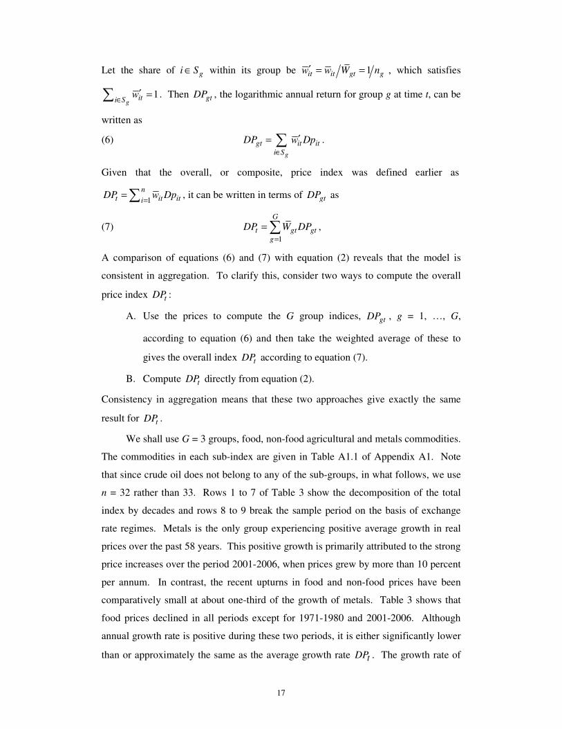
7. Commodities are divided into their respective categories and ranked in ascending
order according to the estimated slope coefficient, iβ , for i = 1, …, 33 (column 4).
All 33 commodities have estimated intercept terms that are statistically insignificant.
The slope coefficient iβ can be used to approximate the overall volatility of an
individual commodity’s return relative to the world commodity market returns.
According to the table, copra has the largest slope coefficient of 2.36, indicating
the price of copra increases by more than 2 percent when the index increases by 1
percent. In other words, copra is very sensitive to worldwide macroeconomic factors.
Conversely, iron ore has an insignificant β of 0.01, implying the price of iron ore is
almost completely insensitive to systematic global factors. One explanation for such a
phenomenon is that iron ore is not traded on the London Metal Exchange unlike the
majority of base metals commodities. Rather, the iron ore prices used in this paper
are contract prices negotiated annually and agreed upon between iron ore producers in
Brazil and steel manufacturers in Europe. By averaging across all commodities, the
mean values for iβ and iα equal one and zero, respectively, as anticipated.
Columns 11 and 12 of Table 7 contain 2R and 21 R− values for each of the
regressions. What stands out is the importance of global risk for the relative prices of
coconut oil ( 2R = 50%) and copra ( 2
R = 54%). More notably, they are the only two
commodities whose global macroeconomic risk factor is greater than 50 percent
30
Table 7
Time-Series Regressions for Annual Growth Rate of 33 Commodities, 1948-2006
Parameters of Return Regressions Risk Component (%)
Intercept iα Slope iβ Regression Statistics
Commodity Coefficient SE Coefficient SE SEE DW Akaike Schwarz F-stat Global
Commodity-
Specific (1) (2) (3) (4) (5) (6) (7) (8) (9) (10) (11) (12)
A. Food Agricultural
1. Bananas -0.73 1.59 0.14 0.15 11.98 2.18 7.84 7.91 0.79 1.39 98.61
2. Oranges -1.50 1.93 0.20 0.19 14.54 2.44 8.23 8.30 1.18 2.07 97.93
3. Beef 0.28 1.60 0.30 0.15 12.05 1.79 7.85 7.92 3.87 6.46 93.54
4. Tea -2.33 2.07 0.50* 0.20 15.63 2.16 8.37 8.44 6.13 * 8.25 91.75
5. Coffee -0.02 3.27 0.73* 0.32 24.65 1.94 9.28 9.35 5.24 * 8.56 91.44
6. Sorghum -0.92 1.39 0.86** 0.14 10.51 2.23 7.58 7.65 40.52 ** 41.98 58.02
7. Wheat -0.96 1.61 0.89** 0.16 12.16 1.78 7.87 7.94 32.59 ** 36.79 63.21
8. Maize -0.48 1.64 0.94** 0.16 12.37 1.88 7.90 7.97 35.25 ** 38.63 61.37
9. Cocoa -1.01 3.19 0.97** 0.31 24.06 1.72 9.23 9.30 9.74 ** 14.82 85.18
10. Soybean meal -1.08 2.46 0.97** 0.24 18.52 2.28 8.71 8.78 16.51 ** 22.77 77.23
11. Groundnut meal -1.48 2.48 1.02** 0.24 17.21 2.26 8.57 8.64 18.55 ** 27.87 72.13
12. Groundnut oil -0.76 2.54 1.07** 0.25 19.17 2.23 8.78 8.85 18.76 ** 25.09 74.91
13. Soybeans -0.68 1.67 1.16** 0.16 12.59 2.32 7.94 8.01 51.53 ** 47.92 52.08
14. Rice -1.12 2.09 1.19** 0.20 15.75 1.80 8.39 8.46 34.68 ** 38.24 61.76
15. Palm oil -1.26 2.40 1.44** 0.23 18.13 2.03 8.67 8.74 38.24 ** 40.58 59.42
16. Sugar 0.74 4.71 1.56** 0.46 35.49 1.96 10.01 10.08 11.76 ** 17.36 82.64
17. Coconut oil 0.05 3.04 2.22** 0.29 22.89 1.85 9.13 9.20 56.77 ** 50.34 49.66
18. Copra 0.10 2.98 2.36** 0.29 22.47 1.90 9.10 9.17 66.52 ** 54.29 45.71 (Table continues on the next page.)

31
Table 7 (continued)
Time-Series Regressions for Annual Growth Rate of 33 Commodities, 1948-2006
Parameters of Return Regressions Risk Component (%)
Intercept iα Slope iβ Regression Statistics
Commodity Coefficient SE Coefficient SE SEE DW Akaike Schwarz F-stat Global
Commodity-
Specific (1) (2) (3) (4) (5) (6) (7) (8) (9) (10) (11) (12)
B. Non-food Agricultural 1. Tobacco -2.44 1.37 0.08 0.13 10.31 2.06 7.54 7.61 0.38 0.68 99.32 2. Jute -2.59 3.25 0.71* 0.31 23.96 2.32 9.23 9.30 5.14 * 8.69 91.31 3. Logs 1.88 2.32 0.91** 0.22 17.48 2.30 8.59 8.66 16.54 ** 22.80 77.20 4. Cotton -1.51 1.95 1.00** 0.19 14.68 2.47 8.25 8.32 27.91 ** 33.26 66.74 5. Rubber 1.35 2.52 1.62** 0.24 19.01 1.94 8.76 8.83 43.66 ** 43.81 56.19
C. Base Metals 1. Iron ore 0.53 1.65 0.01 0.16 12.47 1.19 7.92 7.99 0.00 0.01 99.99 2. Bauxite -0.06 1.72 0.29 0.16 11.49 2.20 7.76 7.84 3.19 6.75 93.25 3. Phosphate rock -0.16 2.73 0.65* 0.27 20.61 1.78 8.92 8.99 6.06 * 9.77 90.23 4. Aluminium 1.06 1.71 0.73** 0.17 12.89 1.91 7.99 8.06 19.32 ** 25.65 74.35 5. Nickel 3.73 2.56 1.06** 0.25 19.29 1.88 8.79 8.86 18.14 ** 24.47 75.53 6. Tin 0.50 1.82 1.23** 0.18 13.70 2.34 8.11 8.18 48.45 ** 46.39 53.61 7. Copper 2.87 2.19 1.50** 0.21 16.52 1.63 8.48 8.55 50.03 ** 47.19 52.81 8. Lead 0.61 2.33 1.51** 0.23 17.61 2.25 8.61 8.68 44.27 ** 44.15 55.85 9. Zinc 2.87 2.43 1.74** 0.24 18.33 1.52 8.69 8.76 54.75 ** 49.44 50.56
D. Oil 1. Crude oil 3.94 3.03 1.30** 0.29 22.85 1.98 9.13 9.20 19.53 ** 25.86 74.14 Mean -0.02 1.00 26.43 73.57
Notes: 1. Double and single asterisks (** and *) denote estimated coefficients significantly different from zero at the 1% and 5% levels,
respectively.
2. SE = standard error. SEE = standard error of the regression. DW = Durbin-Watson statistic.
32
of the total risk. Generally, the 2R values are low, with most of the price variance
explained by risk factors unique to each commodity. The average 2R across the 33
commodities is approximately 26 percent. Commodities whose idiosyncratic risk
accounts for almost all the variations in annual returns over 1948 to 2006 include
banana, iron ore, oranges and tobacco.
An obvious caveat to the above results relates to the sample period, 1948 to
2006 which contains the transition from a period of fixed to floating exchange rate.
As Deaton and Laroque (1992) and Cuddington and Liang (2003) persuasively
demonstrated, primary commodity prices tend to be more volatile under floating than
fixed exchange rates, and the econometric implications of merging data from the two
exchange rate regimes is unclear.10
Therefore, to investigate the effect of a different
exchange rate regime on the results, the sample period is divided into two sub-periods:
(1) pre-1972 (up to and including 1971), corresponding to the fixed exchange rate
regime; and (2) post-1972 (1972 to 2006), corresponding to the floating exchange rate
period. The results shown in Table 8 are ranked in ascending order according to the
estimated β coefficient over the pre-1972 period. There is a large variation in the
estimated β coefficient and the proportion of global risk between the two sub-periods.
Over the pre-1972 sub-period, the estimated β values range from as low as -0.67 for
rice to as high as 3.78 for rubber and are significant for only 12 out of 33 cases
(column 2). Panel A of Figure 8 shows the change in the β coefficient from the pre-
to post-1972 period. The shaded rectangle contains all slope coefficient pairs for each
of the 33 commodities where the base of the shaded rectangle exceeds its height,
implying that the dispersion of β coefficient is much larger in the pre-1972 period.
In addition, 2R is very low during the pre-1972 period, implying the greater part
of the commodity price volatility observed during this sub-period is the result of
idiosyncratic risk factors unique to each primary commodity. Interestingly, 25 out of
the 33 commodities experience increasing 2R values when moving from the pre- to
post-1972 period. Panel B of Figure 8 shows that only eight out of the 33 points lie
below the 45-degree line, which accords with the idea that global risk components
10 Mussa (1986) showed that floating exchange rates have contributed substantially to the variability of
real exchange rate than under the Bretton Woods regime. Since the real appreciation or depreciation
of the US dollar has profound effects on the prices of primary commodities in all other currencies,
higher fluctuations in the exchange rates translate into higher instability of commodity prices. See
Sjaastad and Scacciavillani (1996) and Sjaastad (2008).

33
Table 8
Sensitivity and Risk Components Across Exchange Rate Regime, 1948-2006
1948-1971 1972-2006
iβ Risk Component (%) iβ Risk Component (%)
Commodity Coefficient SE
DW Global
Commodity-
Specific Coefficient SE
DW Global
Commodity-
Specific
iβ Rank (1) (2) (3) (4) (5) (6) (7) (8) (9) (10) (11) (12)
1. Rice -0.67 0.49 1.06 8.25 91.78 1.39** 0.22 2.10 54.26 45.74 25 2. Iron ore -0.33 0.48 1.11 2.19 97.81 0.04 0.18 1.21 0.17 99.83 1 3. Crude oil -0.31 0.38 1.23 3.08 96.92 1.45** 0.37 2.09 31.60 68.40 27 4. Bauxite -0.01 0.42 2.06 0.00 100.00 0.33 0.20 2.31 11.78 88.22 6 5. Aluminium 0.02 0.19 1.25 0.06 99.94 0.81** 0.22 1.92 29.30 70.70 11 6. Nickel 0.03 0.22 1.51 0.09 99.91 1.17** 0.33 1.91 27.75 72.25 22 7. Phosphate rock 0.07 0.39 1.96 0.16 99.84 0.71* 0.35 1.75 11.30 88.70 10 8. Tobacco 0.12 0.48 2.67 0.29 99.71 0.07 0.13 1.53 0.95 99.05 2 9. Tea 0.14 0.53 1.59 0.35 99.65 0.53* 0.24 2.36 13.22 86.79 8
10. Wheat 0.19 0.28 1.43 2.11 97.89 0.96** 0.20 1.85 41.98 58.02 17 11. Maize 0.23 0.52 1.21 0.97 99.03 1.02** 0.17 2.30 53.58 46.42 19 12. Bananas 0.26 0.35 1.68 2.56 97.44 0.12 0.19 2.19 1.20 98.80 4 13. Palm oil 0.30 0.59 2.06 1.23 98.77 1.56** 0.27 1.89 49.75 50.25 30 14. Beef 0.35 0.36 2.02 4.47 95.53 0.31 0.18 1.92 8.29 91.71 5 15. Sorghum 0.51 0.37 2.23 8.27 91.73 0.90** 0.16 2.19 49.77 50.23 14 16. Oranges 1.01 0.63 2.48 10.80 89.20 0.11 0.19 2.42 1.02 98.98 3 17. Coconut oil 1.10 0.66 2.01 11.65 88.35 2.34** 0.36 1.65 56.28 43.72 32 18. Logs 1.25* 0.55 2.43 19.54 80.46 0.88** 0.27 2.24 24.06 75.94 12
19. Cocoa 1.31 1.16 2.04 5.68 94.32 0.93** 0.30 1.32 22.66 77.34 15
20. Groundnut meal 1.35** 0.29 2.67 51.73 48.27 0.98** 0.33 2.21 25.57 74.43 18
(Table continues on the next page.)

34
Table 8 (continued)
Sensitivity and Risk Components Across Exchange Rate Regime, 1948-2006
1948-1971 1972-2006
iβ Risk Component (%) iβ Risk Component (%)
Commodity Coefficient SE
DW Global
Commodity-
Specific Coefficient SE
DW Global
Commodity-
Specific
iβ Rank (1) (2) (3) (4) (5) (6) (7) (8) (9) (10) (11) (12)
21. Tin 1.40** 0.46 2.23 30.79 69.21 1.21** 0.21 2.42 50.58 49.42 23 22. Cotton 1.40** 0.45 1.77 31.45 68.55 0.96** 0.23 2.63 34.52 65.48 16 23. Coffee 1.42* 0.68 1.63 17.09 82.91 0.66 0.39 2.00 7.80 92.20 9 24. Copra 1.43 0.78 2.37 13.89 86.11 2.45** 0.34 1.66 61.64 38.36 33 25. Groundnut oil 1.50** 0.50 1.95 29.85 70.15 1.02** 0.31 2.22 24.77 75.23 20 26. Copper 1.57 0.79 1.85 15.65 84.35 1.50** 0.21 1.41 61.50 38.50 28 27. Soybean meal 1.70** 0.56 2.08 30.95 69.05 0.89** 0.29 2.30 22.33 76.31 13 28. Sugar 1.86 1.55 1.82 6.41 93.59 1.53** 0.48 2.03 23.69 76.31 29 29. Soybeans 2.07** 0.54 2.34 41.24 58.76 1.07** 0.16 2.31 56.33 43.67 21 30. Lead 2.42** 0.70 2.26 35.97 64.03 1.41** 0.24 2.32 50.05 49.95 26 31. Zinc 2.63** 0.72 2.24 38.77 61.23 1.64** 0.26 1.23 55.38 44.62 31 32. Jute 2.90* 1.03 2.16 27.52 72.48 0.48 0.31 2.15 7.21 92.79 7 33. Rubber 3.78** 0.98 2.14 41.62 58.38 1.38** 0.18 1.97 64.61 35.39 24
Mean 1.00 0.99
Notes: 1. Double and single asterisks (** and *) denote estimated coefficients significantly different from zero at the 1% and 5% levels, respectively.
2. Column 12 shows the ranking of each commodity from 1 to 33. Commodity whose rank is higher implies higher estimated β coefficient in
comparison with the remaining commodities in the data set.
3. SE = standard error. DW = Durbin-Watson statistic.

35
Figure 8
Sensitivity and Risk Components Across Exchange Rate Regime, 1948-2006
A. Slope Coefficient, iββββ
012345
-1 0 1 2 3 4 5
B. Share of Global Risk Component, R2 (%)
010203040506070
0 10 20 30 40 50 60 70
have become relatively more important in explaining commodity price volatility
under a floating exchange rate regime. Figure 9 shows that the average 2R values
across 33 commodities increased from 15 percent (Panel A) to 31 percent (Panel B)
between the two sub-periods, indicating that variations in the prices of these
commodities are more closely linked to global macroeconomic factors common to all
1948-1971
1972-2006
45°
1972-2006
1948-1971
45°
Mean = 15%
Mean = 31%
SD = 0.58
SD = 1.04

36
commodities. In other words, systematic risk factors have become more important
over the floating exchange rate regime. The last column of Table 8 is another feature
worthy of note. The column expresses the commodity rank according to its β
coefficient over the second sub-period to assist in cross-commodity comparisons
between the two sub-periods: the higher the rank for the commodity under
investigation, the higher the magnitude of the corresponding β estimates. Of 15
commodities that have estimated β of less than unity over 1948 to 1971, 12
experienced an increase in the level of sensitivity common to global fluctuations in
the second sub-period. Conversely, in 15 out of 18 cases with levels of sensitivity
originally above unity, a decrease in the magnitude of the β coefficient over the two
sub-periods was experienced. As a consequence, the dispersion of β coefficients
among the 33 commodities decreased substantially over the two periods, from 4.45
down to 2.41, the estimated β ranging from as low as 0.04 to 2.45 over the second
sub-period. Overall, the β estimates are not statistically different from one for 20 out
of 33 commodities during the post-1972 period.
Figure 9
Proportion of Common Global Risk in Commodity Price Volatility
A. Fixed Exchange Rate Regime, 1948-1971
Tea Maize Palm oil Wheat Bananas Beef Cocoa Sugar Rice Sorghum Oranges Coconut oil Copra Coffee Groundnut oil Soybean meal SoybeansTobacco Logs Jute Cotton Rubber
Bauxite Aluminum Nickel Phosphate rock Iron ore Copper Tin Lead ZincCrude oil
Groundnut meal
0102030405060
mean = 15%
Commodity
R2
(%)
Food Non-
Food Metals
37
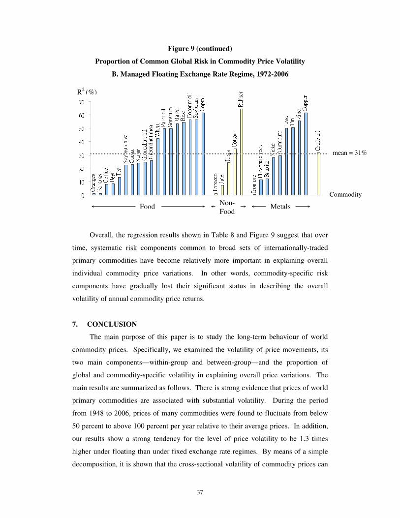
Figure 9 (continued)
Proportion of Common Global Risk in Commodity Price Volatility
B. Managed Floating Exchange Rate Regime, 1972-2006
Oranges Bananas Coffee Beef Tea Soybean meal Cocoa Sugar Groundnut oil Groundnut meal Wheat Palm oil Sorghum Maize Rice Coconut oil Soybeans CopraTobacco Jute Logs Cotton
Rubber
Iron ore Phosphate rock Bauxite Nickel Aluminum Lead Tin Zinc CopperCrude oil
010203040506070
Overall, the regression results shown in Table 8 and Figure 9 suggest that over
time, systematic risk components common to broad sets of internationally-traded
primary commodities have become relatively more important in explaining overall
individual commodity price variations. In other words, commodity-specific risk
components have gradually lost their significant status in describing the overall
volatility of annual commodity price returns.
7. CONCLUSION
The main purpose of this paper is to study the long-term behaviour of world
commodity prices. Specifically, we examined the volatility of price movements, its
two main components—within-group and between-group—and the proportion of
global and commodity-specific volatility in explaining overall price variations. The
main results are summarized as follows. There is strong evidence that prices of world
primary commodities are associated with substantial volatility. During the period
from 1948 to 2006, prices of many commodities were found to fluctuate from below
50 percent to above 100 percent per year relative to their average prices. In addition,
our results show a strong tendency for the level of price volatility to be 1.3 times
higher under floating than under fixed exchange rate regimes. By means of a simple
decomposition, it is shown that the cross-sectional volatility of commodity prices can
mean = 31%
Commodity
R2
(%)
Food Non-
Food Metals

38
be decomposed into within-group and between-group components. The between-
group component accounts for only one-fifth of total price volatility, whereas the
within-group component takes up the remaining four-fifths, indicating that shocks
impacting the commodity market have larger effects on commodities that belong to
the same group, while the spill-over effects to other commodity groups are kept to the
minimum. Finally, the CAPM is used as a loose framework to differentiate global
macroeconomic risk factors from commodity-specific risk in explaining annual
variation in commodity price returns. On average, roughly 31 percent of price
volatility can be attributed to global macroeconomic factors over the period 1972 to
2006, in comparison to 15 percent during the pre-1972 period. In other words, during
the latter period, the other 69 percent of overall variation may be regarded as
commodity-specific risk that can be reduced through proper diversification. In
addition, the estimated β coefficient—the response of commodity return to changes
in world commodity return—moved toward unity in the post-1972 period, implying
that the price of an individual primary commodity increases by one percent when the
overall price index increases by the same amount.
Several qualifications to our results have to be kept in mind. First, this paper
adopts an equal-weighted average price approach in constructing the composite
commodity price index and sub-indices. Second, as pointed out by Valadkhani and
Layton (2006), the portfolio theory underlying CAPM can only be used as a loose
framework in factoring out global risk from commodity specific risk.

39
APPENDIX A1
The Composition of Sub-Indices Over Time
The non-fuel composite price index used in this paper can be further broken
down into three sub-indices including eighteen food commodities, five non-food
agricultural commodities and nine metals commodities. The sub-indices were
selected to analyse the behaviour of commodity prices across different commodity
categories, and to ensure comparability with earlier work. The respective weight of
each group in the composite price index is different depending on the number of non-
fuel primary commodities within each group. As shown in Table A1.1, the weight is
56% for food, 16% for non-food industrial commodities and 28% for metals. Each
primary commodity in question receives equal weight in the price index, therefore its
respective share is fixed throughout the whole sample period except in 1995, 1999
and 2005, when price series were discontinued for bauxite, groundnut meal and jute.
In these instances, the share (i.e., 1/32, as crude oil is excluded from the calculation of
the non-fuel commodity price index) previously assigned to the commodity that was
phased out is evenly distributed among the remaining primary commodities.
See Table A1.2 for details of the expenditure share allocated to each sub-group
over the sample period 1948 to 2006.

40
Table A1.1
Composition of Three Main Sub-Indices
Sub-Category
Food Non-Food Industrial Metals (1) (2) (3)
1. Bananas Cotton Aluminium
2. Beef Jute Bauxite
3. Cocoa Logs Copper
4. Coconut Oil Rubber Iron Ore
5. Coffee Tobacco Lead
6. Copra Nickel
7. Groundnut Meal Phosphate Rock
8. Groundnut Oil Tin
9. Maize Zinc
10. Oranges 11. Palm Oil 12. Rice 13. Sorghum 14. Soybean Meal 15. Soybeans 16. Sugar 17. Tea 18. Wheat
Weight 56.25% 15.63% 28.13%
Note: Weight represents the share of each sub-index within the composite price index.
The index used is an equal-weighted commodity price index.
Table A1.2
Share of Groups Over Time, 1948-2006
Share
Food Non-Food Metals Total
Period
No. of
Commodities 1tW 2tW 3tW 3
1 gtgW
=∑
(1) (2) (3) (4) (5) (6)
1948-1994 32 56.25 15.63 28.13 100.00
1995-1998 31 58.06 16.13 25.81 100.00
1999-2004 30 56.67 16.67 26.67 100.00
2005-2006 29 58.62 13.79 27.59 100.00
Notes: 1. All entries are to be divided by 100.
2. All entries are simple averages over the corresponding periods.
3. Price series for bauxite (metals) were phased out in 1995, groundnut meal
(food) in 1999 and jute (non-food) in 2005.

41
References
Bidarkota, P. and Crucini, M. J. 2000, “Commodity Prices and the Terms of Trade”, Review of International Economics, vol. 8, no. 4, pp. 647-666.
Bomberger, W. A. and Makinen, G. E. 1993, “Inflation and Relative Price Variability:
Parks’ Study Reexamined”, Journal of Money, Credit, and Banking, vol. 25, no. 4, pp. 854-861.
Cashin, P. and McDermott, C. J. 2002, “The Long-Run Behaviour of Commodity
Prices: Small Trends and Big Variability” IMF Working Paper, no. 49. Chan, A. and Clements, K. W. 2007, “The International Volatility of Growth”,
Economics Program Discussion Paper, UWA Business School, The University of Western Australia, no. 07-10, pp. 1-34.
Chu, K. and Morrison, T. K. 1984, “The 1981-82 Recession and Non-Oil Primary
Commodity Prices”, IMF Staff Papers, vol. 31, pp. 93-140. Clements, K. W. 2004, “Three Facts about Marijuana Prices”, Australian Journal of
Agricultural and Resource Economics, vol. 48. no. 2, pp. 271-300. Cuddington, J. T. and Liang, H. 1999, “Commodity Price Volatility Across Exchange
Rate Regimes”, Working Paper. Cuddington, J. T. and Liang, H. 2003, “Commodity Price Volatility Across Exchange
Rate Regimes”, Working Paper. Deaton, A. 1999, “Commodity Prices and Growth in Africa”, The Journal of
Economic Perspectives, vol. 13, no. 3, pp. 23-40. Deaton, A. and Laroque, G. 1992, “On the Behaviour of Commodity Prices”, Review
of Economic Studies, vol. 59, no. 198, pp. 1-23. Grilli, E. R. and Yang, M. C. 1988, “Primary Commodity Prices, Manufactured
Goods Prices, and the Terms of Trade of Developing Countries: What the Long Run Shows”, The World Bank Economic Review, vol. 2, no. 1, pp. 1-47.
Jaramillo, C. F. 1999, “Inflation and Relative Price Variability: Reinstating Parks’
Results”, Journal of Money, Credit, and Banking, vol. 31, no. 3, pp. 375-385. Kroner, K. F., Kneafsey, D. P. and Claessens, S. 1993, “Forecasting Volatility in
Commodity Markets”, World Bank Policy Research Working Paper, no. 1226. Lintner, J. 1965, “The Valuation of Risk Assets and Selection of Risky Investments in
Stock Portfolios and Capital Budgets”, Review of Economics and Statistics, vol. 47, pp. 13-37.
Markowitz, H. 1959, Portfolio Selection: Efficient Diversification of Investments,
Wiley, New York. Mossin, J. 1966, “Equilibrium in Capital Market”, Econometrica, vol. 34, pp. 768-783. Mussa, M. 1986, “Nominal Exchange Rate Regimes and the Behavior of Real
Exchange Rates: Evidence and Implications”, Carnegie-Rochester Conference Series on Public Policy, North Holland Publishing Company, Amsterdam, no. 25, pp.117-213.

42
Parks, R. W. 1978, “Inflation and Relative Price Variability”, Journal of Political
Economy, vol. 86, no. 1, pp. 79-95. Pindyck, R. S. 2001, “Volatility and Commodity Price Dynamics”, Center for Energy
and Environmental Policy Research Working Paper, no. 01-007. Pfaffenzeller, S., Newbold, P. and Rayner, A. 2007, “A Short Note on Updating the
Grilli and Yang Commodity Price Index”, The World Bank Economic Review, vol. 21, no. 1, pp. 151-163.
Reinhart, C. M. and Wickham, P. 1994, “Commodity Prices: Cyclical Weakness or
Secular Decline? ”, IMF Staff Papers, vol. 41, pp. 175-213. Sharp, W. F. 1964, “Capital Asset Prices: A Theory of Market Equilibrium
Conditions of Risk”, Journal of Finance, vol. 19, pp. 425-442. Sjaastad, L. A. 2008, “The Price of Gold and the Exchange Rates: Once Again”,
Resources Policy, vol. 33, pp. 118-124. Sjaastad, L. and Scacciavillani, F. 1996, “The Price of Gold and the Exchange Rate”,
Journal of International Money and Finance, vol. 15, pp. 879-897. Valadkhani, A. and Layton, A. 2006, “A Cross-Country Analysis of Export Prices in
OECD Countries”, Economic Papers, vol. 25, no. 4, pp. 331-346. Vining, D. R., Jr. and Elwertowski, T. C. 1976, “The Relationship between Relative
Prices and the General Price Level”, The American Economic Review, vol. 66, no. 4, pp. 699-708.
Yamey, B. S. 1992, “The Tin Crisis (1985-86) and Futures Trading”, Economic
Record, vol. 68, pp. 10-15.