Economics of the Firm

Strategic Pricing Techniques

Market Structures

Recall that there is an entire spectrum of market structures

Perfect CompetitionMany firms, each with zero market shareP = MCProfits = 0 (Firm’s earn a reasonable rate of return on invested capital)NO STRATEGIC INTERACTION!

MonopolyOne firm, with 100% market shareP > MCProfits > 0 (Firm’s earn excessive rates of return on invested capital)NO STRATEGIC INTERACTION!

Most industries, however, don’t fit the assumptions of either perfect competition or monopoly. We call these industries oligopolies

OligopolyRelatively few firms, each with significant market shareSTRATEGIES MATTER!!!

Wireless (2002)Verizon: 30% Cingular: 22% AT&T: 20% Sprint PCS: 14% Nextel: 10% Voicestream: 6%

US Beer (2001)Anheuser-Busch: 49% Miller: 20% Coors: 11% Pabst: 4% Heineken: 3%

Music Recording (2001)Universal/Polygram: 23% Sony: 15% EMI: 13% Warner: 12% BMG: 8%

Market shares are not constant over time in these industries!

9

11

14

15

20

21

Airlines (1992) Airlines (2002)

American

Northwest

Delta

United

Continental

US Air 7

9

11

15

17

19American

United

Delta

Northwest

Continental

SWest

While the absolute ordering didn’t change, all the airlines lost market share to Southwest.

Another trend is consolidation

44

55

677

888

9

Retail Gasoline (1992) Retail Gasoline (2001)

Shell

ExxonTexaco

Chevron

Amoco

Mobil

7

10

16

18

20

24Exxon/Mobil

Shell

BP/Amoco/Arco

Chev/Texaco

Conoco/PhillipsCitgoBP

Marathon

SunPhillips

Total/Fina/Elf

The key difference in oligopoly markets is that price/sales decisions can’t be made independently of your competitor’s decisions

Monopoly

PQQ Oligopoly

NPPPQQ ,..., 1

Your Price (-)

Your N Competitors Prices (+)

Oligopoly markets rely crucially on the interactions between firms which is why we need game theory to analyze them!

Strategy Matters!!!!!

Prisoner’s Dilemma…A Classic!

Jake

Two prisoners (Jake & Clyde) have been arrested. The DA has enough evidence to convict them both for 1 year, but would like to convict them of a more serious crime.

Clyde

The DA puts Jake & Clyde in separate rooms and makes each the following offer:

Keep your mouth shut and you both get one year in jail

If you rat on your partner, you get off free while your partner does 8 years

If you both rat, you each get 4 years.

Jake

Clyde

Confess Don’t Confess

Confess -4 -4 0 -8

Don’t Confess

-8 0 -1 -1

Jake is choosing rows Clyde is choosing columns

Jake

Clyde

Confess Don’t Confess

Confess -4 -4 0 -8

Don’t Confess

-8 0 -1 -1

Suppose that Jake believes that Clyde will confess. What is Jake’s best response?

If Clyde confesses, then Jake’s best strategy is also to confess

Jake

Clyde

Confess Don’t Confess

Confess -4 -4 0 -8

Don’t Confess

-8 0 -1 -1

Suppose that Jake believes that Clyde will not confess. What is Jake’s best response?

If Clyde doesn’t confesses, then Jake’s best strategy is still to confess

Jake

Clyde

Confess Don’t Confess

Confess -4 -4 0 -8

Don’t Confess

-8 0 -1 -1

Dominant Strategies

Jake’s optimal strategy REGARDLESS OF CLYDE’S DECISION is to confess. Therefore, confess is a dominant strategy for Jake

Note that Clyde’s dominant strategy is also to confess

Nash Equilibrium

Jake

Clyde

Confess Don’t Confess

Confess -4 -4 0 -8

Don’t Confess

-8 0 -1 -1

The Nash equilibrium is the outcome (or set of outcomes) where each player is following his/her best response to their opponent’s moves

Here, the Nash equilibrium is both Jake and Clyde confessing

“Winston tastes good like a cigarette should!”

“Us Tareyton smokers would rather fight than switch!”

Advertise Don’t Advertise

Advertise 10 10 30 5

Don’t Advertise

5 30 20 20

How about this game?

$.95 $1.30 $1.95

$1.00 3 6 7 3 10 4

$1.35 5 1 8 2 14 7

$1.65 6 0 6 2 8 5

Alli

ed

Acme

Acme and Allied are introducing a new product to the market and need to set a price. Below are the payoffs for each price combination.

What is the Nash Equilibrium?

Iterative Dominance

$.95 $1.30 $1.95

$1.00 3 6 7 3 10 4

$1.35 5 1 8 2 14 7

$1.65 6 0 6 2 8 5

Alli

ed

Acme

Note that Allied would never charge $1 regardless of what Acme charges ($1 is a dominated strategy). Therefore, we can eliminate it from consideration.

With the $1 Allied Strategy eliminated, Acme’s strategies of both $.95 and $1.30 become dominated.

With Acme’s strategies reduced to $1.95, Allied will respond with $1.35

Repeated GamesJake Clyde

The previous example was a “one shot” game. Would it matter if the game were played over and over?

Suppose that Jake and Clyde were habitual (and very lousy) thieves. After their stay in prison, they immediately commit the same crime and get arrested. Is it possible for them to learn to cooperate?

Time0 1 2 3 4 5

Play PD Game

Play PD Game

Play PD Game

Play PD Game

Play PD Game

Play PD Game

Repeated GamesJake Clyde

Time0 1 2 3 4 5

Play PD Game

Play PD Game

Play PD Game

Play PD Game

Play PD Game

Play PD Game

We can use backward induction to solve this.

At time 5 (the last period), this is a one shot game (there is no future). Therefore, we know the equilibrium is for both to confess.

Confess Confess

However, once the equilibrium for period 5 is known, there is no advantage to cooperating in period 4

Confess Confess

Confess Confess

Confess Confess

Confess Confess

Confess Confess

Similar arguments take us back to period 0

Infinitely Repeated Games Jake Clyde

0 1 2

Play PD Game

Play PD Game

Play PD Game ……………

Suppose that Jake knows Clyde is planning on NOT CONFESSING at time 0.

Option #1: Don’t confess, get 1 year in jail (rather than 0 if he confesses), but establish trust for the next time

Option #2: Confess, get 0 years in jail (rather than 1 if he doesn’t confess), but ruins trust for the next time

You need to value the future for this option to be viable

Suppose that McDonald’s is currently the only restaurant in town, but Burger King is considering opening a location. Should McDonald's fight for it’s territory?

IN

Out

Fight

Cooperate

0

2

1

5

0

2

Now, suppose that this game is played repeatedly. That is, suppose that McDonald's faces possible entry by burger King is 20 different locations. Can entry deterrence be a credible strategy?

Enter Enter EnterDon’t Fight

Don’t Fight

Don’t Fight

2

Enter Don’t Enter

Don’t Enter

Fight Don’t Enter

Don’t Enter

0

OR

2 2

5 5 5 5

Total =2*20 = 40

Total =19*5 = 95

Enter

Don’t Enter

Enter

Don’t Enter

Enter

Don’t Enter

Fight

Don’t Fight

Fight

Don’t Fight

Fight

Don’t Fight

End of Time

Does McDonald’s have an incentive to fight here?

What will Burger King do here?

If there is an “end date” then McDonald's threat loses its credibility!!

Now, suppose that this game is played repeatedly. That is, suppose that McDonald's faces possible entry by burger King is 20 different locations. Can entry deterrence be a credible strategy?

Don’t Audit

Audit

Cheat 5 -5 -25 5

Don’t Cheat

0 0 -1 -1

What is the equilibrium to this game?

Ever Cheat on your taxes?

In this game you get to decide whether or not to cheat on your taxes while the IRS decides whether or not to audit you

If the IRS never audited, your best strategy is to cheat (this would only make sense for the IRS if you never cheated)

The Equilibrium for this game will involve mixed strategies!

Don’t Audit

Audit

Cheat 5 -5 -25 5

Don’t Cheat

0 0 -1 -1

If the IRS always audited, your best strategy is to never cheat (this would only make sense for the IRS if you always cheated)

A quick detour: Expected Value

Suppose that I offer you a lottery ticket: This ticket has a 2/3 chance of winning $100 and a 1/3 chance of losing $100. How much is this ticket worth to you?

Suppose you played this ticket 6 times:

Attempt Outcome

1 $100

2 $100

3 -$100

4 $100

5 -$100

6 $100

Total Winnings: $200Attempts: 6Average Winnings: $200/6 = $33.33

A quick detour: Expected Value

Given a set of probabilities, Expected Value measures the average outcome

Expected Value = A weighted average of the possible outcomes where the weights are the probabilities assigned to each outcome

Suppose that I offer you a lottery ticket: This ticket has a 2/3 chance of winning $100 and a 1/3 chance of losing $100. How much is this ticket worth to you?

33.33$100$3

1100$

3

2

EV

Cheating on your taxes!

Don’t Audit

Audit

Cheat 5 -5 -25 5

Don’t Cheat

0 0 -1 -1

Suppose that the IRS Audits 25% of all returns. What should you do?

Cheat: 5.22525.575. EV

Don’t Cheat: 25.125.075. EV

If the IRS audits 25% of all returns, you are better off not cheating. But if you never cheat, they will never audit, …

Don’t Audit Audit

Cheat 5 -5 -25 5

Don’t Cheat 0 0 -1 -1

The only way this game can work is for you to cheat sometime, but not all the time. That can only happen if you are indifferent between the two!

Cheat: 255 ADA ppEV

Don’t Cheat: 10 ADA PpEV

Suppose the government audits with probability Ap

Doesn’t audit with probability DAp

If you are indifferent…

DAA

ADA

AADA

pp

pp

ppp

24

5

245

255

1 DAA pp

29

24

124

29

124

5

DA

DA

DADA

p

p

pp

(83%)29

5Ap (17%)

Don’t Audit Audit

Cheat 5 -5 -25 5

Don’t Cheat 0 0 -1 -1

We also need for the government to audit sometime, but not all the time. For this to be the case, they have to be indifferent!

Audit: 51 CDC ppEV

Don’t Audit: 50 CDC PpEV

Suppose you cheat with probability Cp

Don’t cheat with probability DCp

If they are indifferent…

DCC

DCC

CDCC

pp

pp

ppp

10

1

10

55

1 DCC pp

11

10

110

11

110

1

DC

DC

DCDC

p

p

pp

(91%)11

1Ap (9%)

Don’t Audit Audit

Cheat 5 -5 -25 5

Don’t Cheat 0 0 -1 -1

Now we have an equilibrium for this game that is sustainable!

The government audits with probability %17ApDoesn’t audit with probability %83DAp

Suppose you cheat with probability %9Cp

Don’t cheat with probability %91DCp

We can find the odds of any particular event happening….

You Cheat and get audited: 0153.17.09. AC pp (1.5%)

(1.5%)(7.5%)

(15%)(75%)

The Airline Price Wars

p

Q

$500

$220

60 180

Suppose that American and Delta face the given demand for flights to NYC and that the unit cost for the trip is $200. If they charge the same fare, they split the market

P = $500 P = $220

P = $500 $9,000

$9,000

$3,600

$0

P = $220 $0

$3,600

$1,800

$1,800

American

Del

taWhat will the equilibrium be?

The Airline Price Wars

P = $500 P = $220

P = $500 $9,000

$9,000

$3,600

$0

P = $220 $0

$3,600

$1,800

$1,800

American

Del

ta

If American follows a strategy of charging $500 all the time, Delta’s best response is to also charge $500 all the time

If American follows a strategy of charging $220 all the time, Delta’s best response is to also charge $220 all the time

This game has multiple equilibria and the result depends critically on each company’s beliefs about the other company’s strategy

The Airline Price Wars: Mixed Strategy Equilibria

P = $500 P = $220

P = $500 $9,000

$9,000

$3,600

$0

P = $220 $0

$3,600

$1,800

$1,800

American

Del

ta

Charge $500: 09000 LH ppEV

Charge $220: 18003600 LH PpEV

Suppose American charges $500 with probability Hp

Charges $220 with probability Lp

LHH ppp 180036009000

HL pp 3

4

3Lp

4

1Hp(75%) (25%)

(56%)(19%)

(19%)(6%)

Suppose that we make the game sequential. That is, one side makes its decision (and that decision is public) before the other

Che

at

Aud

it

Aud

it

Don’t

Cheat

Don’t

Audit

Don’t

Audit

(-25, 5) (5, -5)(-1, -1) (0, 0)

Don’t Audit Audit

Cheat 5 -5 -25 5

Don’t Cheat 0 0 -1 -1

Your reward is on the left

If the IRS observes you cheating, their best choice is to Audit

Che

at

Aud

it

Aud

it

Don’t

Cheat

Don’t

Audit

Don’t

Audit

(-25, 5) (5, -5)(-1, -1) (0, 0)

Don’t Audit Audit

Cheat 5 -5 -25 5

Don’t Cheat 0 0 -1 -1

Your reward is on the leftvs

If the IRS observes you not cheating, their best choice is to not audit

Che

at

Aud

it

Aud

it

Don’t

Cheat

Don’t

Audit

Don’t

Audit

(-25, 5) (5, -5)(-1, -1) (0, 0)

Don’t Audit Audit

Cheat 5 -5 -25 5

Don’t Cheat 0 0 -1 -1

Your reward is on the leftvs

Knowing how the IRS will respond, you never cheat and they never audit!!

Che

at

Aud

it

Aud

it

Don’t

Cheat

Don’t

Audit

Don’t

Audit

(-25, 5) (5, -5)(-1, -1) (0, 0)

Don’t Audit Audit

Cheat 5 -5 -25 5

Don’t Cheat 0 0 -1 -1

Your reward is on the leftvs

(0%)(0%)

(0%)(100%)

Now, lets switch positions…suppose the IRS chooses first

Aud

it

Che

at

Che

at

Don’t

Audit

Don’t

Cheat

Don’t

Cheat

(-25, 5) (-1, -1)(5, -5) (0, 0)

Don’t Audit Audit

Cheat 5 -5 -25 5

Don’t Cheat 0 0 -1 -1

Your reward is on the left

(0%)(0%)

(100%)(0%)

Again, we could play this game sequentially

$500

$500

$500

$220

$220

$220

(9,000, 9,000) (3,600, 0) (0, 3,600) (1,800, 1,800)

Delta’s reward is on the left

P = $500 P = $220

P = $500 $9,000

$9,000

$3,600

$0

P = $220 $0

$3,600

$1,800

$1,800

(0%)(100%)

(0%)(0%)

Note: Even if the moves are made sequentially, if one party is not aware of the other’s move, we are back to the simultaneous move game

Che

at

Aud

it

Aud

it

Don’t

Cheat

Don’t

Audit

Don’t

Audit

(-25, 5) (5, -5)(-1, -1) (0, 0)

i.e., Al Capone might have cheated all the time, but if the IRS is unaware, they might not audit all the time!

Terrorists

Terrorists

President

Take

H

osta

ges

Neg

otia

te

Kill

Don’t Take

Hostages

Don’t K

ill

Don’t

Negotiate

(1, -.5)

(-.5, -1) (-1, 1)

(0, 1)

In the Movie Air Force One, Terrorists hijack Air Force One and take the president hostage. Can we write this as a game? (Terrorists payouts on left)

In the third stage, the best response is to kill the hostages

Given the terrorist response, it is optimal for the president to negotiate in stage 2

Given Stage two, it is optimal for the terrorists to take hostages

Terrorists

Terrorists

President

Take

H

osta

ges

Neg

otia

te

Kill

Don’t Take

Hostages

Don’t K

ill

Don’t

Negotiate

(1, -.5)

(-.5, -1) (-1, 1)

(0, 1)

The equilibrium is always (Take Hostages/Negotiate). How could we change this outcome?

Suppose that a constitutional amendment is passed ruling out hostage negotiation (a commitment device)

Without the possibility of negotiation, the new equilibrium becomes (No Hostages)

A bargaining example…How do you divide $20?

Two players have $20 to divide up between them. On day one, Player A makes an offer, on day two player B makes a counteroffer, and on day three player A gets to make a final offer. If no agreement has been made after three days, both players get $0.

Player A

Player B

Offer

Accept Reject

Player B

Offer

Player A

Accept Reject

Player A

Offer

Player B

Accept Reject

(0,0)

Day 1

Day 2

Day 3

Player A

Player B

Offer

Accept Reject

Player B

Offer

Player A

Accept Reject

Player A

Offer

Player B

Accept Reject

(0,0)

Day 1

Day 2

Day 3

If day 3 arrives, player B should accept any offer – a rejection pays out $0!

Player A: $19.99Player B: $.01

Player B knows what happens in day 3 and wants to avoid that!

Player A: $19.99Player B: $.01

Player A knows what happens in day 2 and wants to avoid that!

Player A: $19.99Player B: $.01

Player A

Player B

Offer

Accept Reject

Player B

Offer

Player A

Accept Reject

Player A

Offer

Player B

Accept Reject

(0,0)

Day 1

Day 2

Day 3

Lets consider a couple variations…

Variation #1: Negotiations take a lot of time and each player has an opportunity cost of waiting:

•Player A has an investment opportunity that pays 20% per year.•Player B has an investment strategy that pays 10% per year

Player A

Player B

Offer

Accept Reject

Player B

Offer

Player A

Accept Reject

Player A

Offer

Player B

Accept Reject

(0,0)

Year 1

Year 2

Year 3

If year 3 arrives, player B should accept any offer – a rejection pays out $0!

Player A: $19.99Player B: $.01

If player A rejects, she gets $19.99 in one year. That’s worth $19.99/1.20 today

Player A: $16.65Player B: $3.35

If player B rejects, she gets $3.35 in one year. That’s worth $3.35/1.10 today

Player A: $16.95Player B: $3.05

Continuous Choice Games

Consider the following example. We have two competing firms in the marketplace.

These two firms are selling identical products. Each firm has constant marginal costs of production.

What are these firms using as their strategic choice variable? Price or quantity?

Are these firms making their decisions simultaneously or is there a sequence to the decisions?

Cournot Competition: Quantity is the strategic choice variable

p

QD

There are two firms in an industry – both facing an aggregate (inverse) demand curve given by

Total Industry Production

Both firms have constant marginal costs equal to $20

21 qqQ

QP 20120

From firm one’s perspective, the demand curve is given by

1221 202012020120 qqqqP

Treated as a constant by Firm One

Solving Firm One’s Profit Maximization…

204020120 12 qqMR

40

20100 21

qq

In Game Theory Lingo, this is Firm One’s Best Response Function To Firm 2

1q

2q

40

20100 21

qq

05.2

0

1

2

q

q

If firm 2 drops out, firm one is a monopolist!

5.2

2040120

20120

1

1

1

q

qMR

qP

1q

2q

40

20100 21

qq

What could firm 2 do to make firm 1 drop out?

5.2

0

1

2

q

q

0

5

1

2

q

q

MCP 20520120

1q

2q 40

20100 21

qq

5.2

0

1

2

q

q

0

5

1

2

q

q

3

1

Firm 2 chooses a production target of 3

Firm 1 responds with a production target of 1

QP 20120

40420120 P

60320340

20120140

2

1

The game is symmetric with respect to Firm two…

1q

2q40

20100 12

qq

5.2

0

2

1

q

q

0

5

2

1

q

q

Firm 1 chooses a production target of 1

Firm 2 responds with a production target of 2

QP 20120

60320120 P

160220260

40120160

2

1

1q

2q

Firm 1

Firm 2

67.1*

1q

67.1*2 q

Eventually, these two firms converge on production levels such that neither firm has an incentive to change

40

20100 12

qq

40

20100 21

qq

40

67.12010067.1

We would call this the Nash equilibrium for this model

Recall we started with the demand curve and marginal costs

20

20120

MC

QP

Mqq 67.1*2

*1

33.53$)33.3(20120 P

66.55$67.12067.133.53

66.55$67.12067.133.53

2

1

The markup formula works for each firm

33.53$)67.1(206.86

67.1*

P

MQ

1

1

MCp

6.167.1

33.53

20

1

iQ

P

P

Q

6.11

1

20$33.53$

20$

206.862020120 112

MC

qqqP

Had this market been serviced instead by a monopoly,

70$)5.2(20120

5.2*

P

MQ

20$

20120

MC

QP

1

1

MCp

4.15.2

70

20

1

Q

P

P

Q

4.11

1

20$70$

Had this market been instead perfectly competitive,

20$)5.2(20120

5*

P

MQ

20$

20120

MC

QP

1

1

MCp

1

1

20$20$

20$

20120

MC

QP

Monopoly

000,10

5.2

70$

5.2*

HHI

LI

P

MQ

Perfect Competition

0

0

20$

5*

HHI

LI

P

MQ

2 Firms

000,5

65.1

53$

67.1

33.3

HHI

LI

P

q

MQ

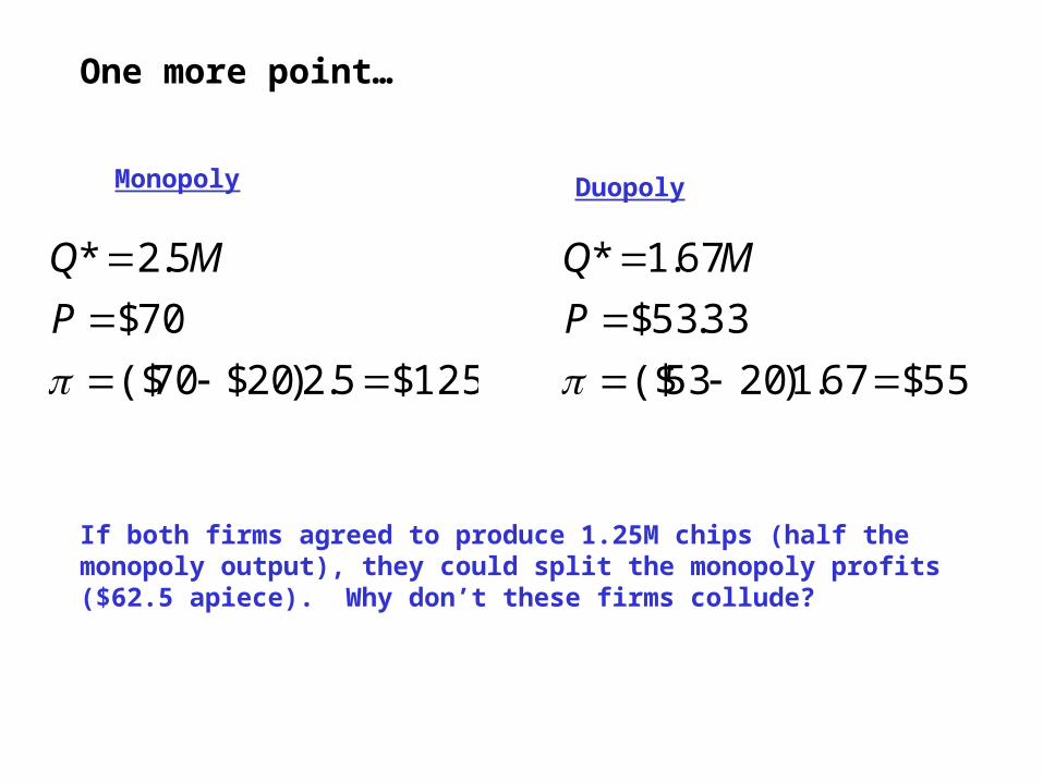
One more point…

125$5.2)20$70($

70$

5.2*

P

MQ

55$67.1)2053($

33.53$

67.1*

P

MQ

Monopoly Duopoly

If both firms agreed to produce 1.25M chips (half the monopoly output), they could split the monopoly profits ($62.5 apiece). Why don’t these firms collude?

Suppose we increase the number of firms…say, to 3

QP 20120

Demand facing firm 1 is given by (MC = 20)

32120120 qqqP

132 202020120 qqqP

20402020120 132 qqqMR

40

2020100 321

qqq

The strategies look very similar!

Expanding the number of firms in an oligopoly – Cournot Competition

BN

cAqi )1(

BN

cANQ

)1(

cN

N

N

AP

11

Note that as the number of firms increases:Output approaches the perfectly competitive level of production Price approaches marginal cost.

Lets go back to the previous example…

cMC

BQAP

20$

20120

MC

QP

p

QD

$70

2.5

CS = (.5)(120 – 70)(2.5) = $62.5

$62.5

What would it be worth to consumers to add another firm to the industry?

Recall, we had an aggregate demand and a constant marginal cost of production.

Monopoly$120

000,10

5.2

70$

5.2*

HHI

LI

P

MQ

20$

20120

MC

QP

p

QD

$53

3.33

CS = (.5)(120 – 53)(3.33) = $112

$112

Recall, we had an aggregate demand for computer chips and a constant marginal cost of production.

000,5

65.1

53$

67.1

33.3

HHI

LI

P

q

MQ

Two Firms

20$

20120

MC

QP

p

QD

$45

3.75

CS = (.5)(120 – 45)(3.75) = $140

$140

267,3

25.1

45$

75.33

25.1

HHI

LI

P

qQ

Mqi

With three firms in the market…

Three Firms

0

10

20

30

40

50

60

70

80

0

1

2

3

4

5

6

Number of Firms

Firm Sales Industry Sales Price

Increasing Competition

Increasing Competition

0

50

100

150

200

250

300

Number of Firms

Consumer Surplus Firm Profit Industry Profit

20$

20120

MC

QP

Now, suppose that there were annual fixed costs equal to $10

How many firms can this industry support?

BN

cAqi )1(

c

N

N

N

AP

11

010$)20$( ii qP Solve for N

0

10

20

30

40

50

60

70

80

90

100

110

120

130

140

1 2 3 4 5 6 7 8 9 10 11 12 13 14 15 16 17 18 19 20 21 22 23 24 25

With a fixed cost of $10, this industry can support 7 Firms

1q

2q

Firm 1

Firm 2

The previous analysis was with identical firms.

67.1*2 q

67.1*1 q

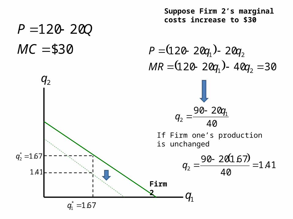
Suppose Firm 2’s marginal costs increase to $30

20$

20120

MC

QP40

20100 12

qq

40

20100 21

qq

50%

50%

1q

2q

Firm 2

67.1*2 q

67.1*1 q

30$

20120

MC

QP

304020120

2020120

21

21

qqMR

qqP

Suppose Firm 2’s marginal costs increase to $30

40

2090 12

qq

If Firm one’s production is unchanged

41.1

40

67.120902

q

41.1

1q

2q

Firm 1

Firm 233.12 q

83.1*1 q

Firm 2’s market share drops

42%

58%

40

2090 12

qq

40

20100 21

qq

64.3533.13033.18.56

34.6783.12083.18.56

8.56$16.320120

16.383.133.1

2

1

P

Q

27.1

51285842 22

LI

HHI

1q

2q

Firm 1

Firm 233.12 q

83.1*1 q

Firm 2’s market share drops

42%

58%

The Process…

With a rise in marginal costs, Firm 2’s profit margins shrink

To bring profit margins back up, Firm 2 lowers production levels which lowers industry output and raises the price

A higher price raises Firm 1’s profit margins. This causes them to expand production

The previous analysis (Cournot Competition) considered quantity as the strategic variable. Bertrand competition uses price as the strategic variable.

p

QD

Q*

P*

Should it matter?

QP 20120 Just as before, we have an industry demand curve and two competing duopolies – both with marginal cost equal to $20.Industry Output

1qD

12 2020120 qqP PQ 05.6 Quantity Strategy

1p

1qD

Bertrand Case

220120 q

p

2p

Firm level demand curves look very different when we change strategic variables

If you are underpriced, you lose the whole market

If you are the low price you capture the whole market

At equal prices, you split the market

Price competition creates a discontinuity in each firm’s demand curve – this, in turn creates a discontinuity in profits

2111

211

1

21

211

)05.6)(20(

2

05.6)20(

0

,

ppifpp

ppifp

p

ppif

pp

As in the cournot case, we need to find firm one’s best response (i.e. profit maximizing response) to every possible price set by firm 2.

Firm One’s Best Response Function

mpp 2

Case #1: Firm 2 sets a price above the pure monopoly price:

220 pCase #3: Firm 2 sets a price below marginal cost

202 ppm

Case #2: Firm 2 sets a price between the monopoly price and marginal cost

mpp 1

21 pp

21 pp

2pc Case #4: Firm 2 sets a price equal to marginal cost

cpp 21

What’s the Nash equilibrium of this game?

However, the Bertrand equilibrium makes some very restricting assumptions…

Firms are producing identical products (i.e. perfect substitutes)Firms are not capacity constrained

Monopoly

000,10

5.2

70$

5.2*

HHI

LI

P

MQ

Perfect Competition

0

0

20$

5*

HHI

LI

P

MQ

2 Firms

000,5

0

20$

5.2

5

HHI

LI

P

q

MQ

An example…capacity constraints

Consider two theatres located side by side. Each theatre’s marginal cost is constant at $10. Both face an aggregate demand for movies equal to

PQ 60000,6 Each theatre has the capacity to handle 2,000 customers per day.

What will the equilibrium be in this case?

PQ 60000,6 If both firms set a price equal to $10 (Marginal cost), then market demand is 5,400 (well above total capacity = 2,000)

Note: The Bertrand Equilibrium (P = MC) relies on each firm having the ability to make a credible threat:

“If you set a price above marginal cost, I will undercut you and steal all your customers!”

33.33$

60000,6000,4

P

P

At a price of $33, market demand is 4,000 and both firms operate at capacity

With competition in price, the key is to create product variety somehow! Suppose that we have two firms. Again, marginal costs are $20. The two firms produce imperfect substitutes.

80

40121

ppq

80

40212

ppq

1qD

1

p

402 p

11 0125.1 pq

Product Differentiation

Recall Firm 1 has a marginal cost of $20

80

40)20( 12

11

ppp

Each firm needs to choose price to maximize profits conditional on the other firm’s choice of price.

21 5.30 pp

Firm 1 profit maximizes by choice of price

1pD

2p

Firm 1’s strategy

$30

Firm 2 sets a price of $50

Firm 1 responds with $55

1p

2p

Firm 1

Firm 2

30$

30$

60$

60$

80

40121

ppq

80

40212

ppq

With equal costs, both firms set the same price and split the market evenly

Monopoly

000,10

5.2

70$

5.2*

HHI

LI

P

MQ

Perfect Competition

0

0

20$

5*

HHI

LI

P

MQ

2 Firms

000,5

2

60$

HHI

LI

P

50.1 q

50.2 q

60$1 p

60$2 p

1p

2p

Firm 2

Suppose that Firm two‘s costs increase. What happens in each case?

Bertrand

$30

80

40)20( 11

22

ppp

With higher marginal costs, firm 2’s profit margins shrink. To bring profit margins back up, firm two raises its price

1p

2pFirm 1

Firm 2

Suppose that Firm two‘s costs increase. What happens in each case?

With higher marginal costs, firm 2’s profit margins shrink. To bring profit margins back up, firm two raises its price

A higher price from firm two sends customers to firm 1. This allows firm 1 to raise price as well and maintain market share!

Cournot (Quantity Competition): Competition is for market shareFirm One responds to firm B’s cost increases by expanding production and increasing market shareBest response strategies are strategic substitutes

Bertrand (Price Competition): Competition is for profit marginFirm One responds to firm B’s cost increases by increasing price and maintaining market shareBest response strategies are strategic complements

1p

2pFirm 1

Firm 2

1q

2q

Firm 1

Firm 2

Bertrand Cournot

Stackelberg leadership

In the previous example, firms made price/quantity decisions simultaneously. Suppose we relax that and allow one firm to choose first.

20

20120

MC

QP

Both firms have a marginal cost equal to $20

Firm A chooses its output first

Firm B chooses its output second

Market Price is determined

Firm B has observed Firm A’s output decision and faces the residual demand curve:

21 2020120 qqP

40

20100 12

qq

204020120 21 qqMR

1q

5.2

0

1

2

q

q

0

5

1

2

q

q

2q

Knowing Firm B’s response, Firm A can now maximize its profits:

12 2020120 qqP

5.2

202070

1070

1

1

1

q

qMR

qPFirm 1 produces the monopoly output!

40

20100 12

qq

5.21 q 45$75.320120

75.3

P

Q

25.140

20100 12

qq

25.3125.12025.145

50.625.2205.245

2

1

Monopoly

000,10

5.2

70$

5.2*

HHI

LI

P

MQ

Perfect Competition

0

0

20$

5*

HHI

LI

P

MQ

2 Firms

587,5

25.1

45$

25.1

5.2

75.3

2

1

HHI

LI

P

q

q

MQ(67%)

(33%)

Sequential Bertrand Competition

We could also sequence events using price competition.

80

40121

ppq

80

40212

ppq

Product Differentiation

Both firms have a marginal cost equal to $20

Firm 2 chooses its price first

Firm 2 chooses its price second

Market sales are determined

38.1 qSequential Bertrand Competition

80$1 p

70$2 p 62.2 q

Monopoly

000,10

5.2

70$

5.2*

HHI

LI

P

MQ

Perfect Competition

0

0

20$

5*

HHI

LI

P

MQ

2 Firms

288,5

75.2

75$

62.

38.

2

1

HHI

LI

P

q

q

Cournot vs. Bertrand: Stackelberg Games

Cournot (Quantity Competition): Firm One has a first mover advantage – it gains market share

and earns higher profits. Firm B loses market share and earns lower profits

Total industry output increases (price decreases)

Bertrand (Price Competition):Firm Two has a second mover advantage – it charges a lower price (relative to firm one), gains market share and increases profits.Overall, production drops, prices rise, and both firms increase profits.

Campbell’s Soup has accounted for 60% of the canned soup market for over 50 years

Market Dominance

Sotheby’s and Christie’s have controlled 90% of the auction market for two decades (each holds 50% of its own domestic market)

Intel has held 90% of the computer chip market for 10 years.

Microsoft has held 90% of the operating system market over the last 10 years

On average, the number one firm in an industry retains that rank for 17 – 28 years!

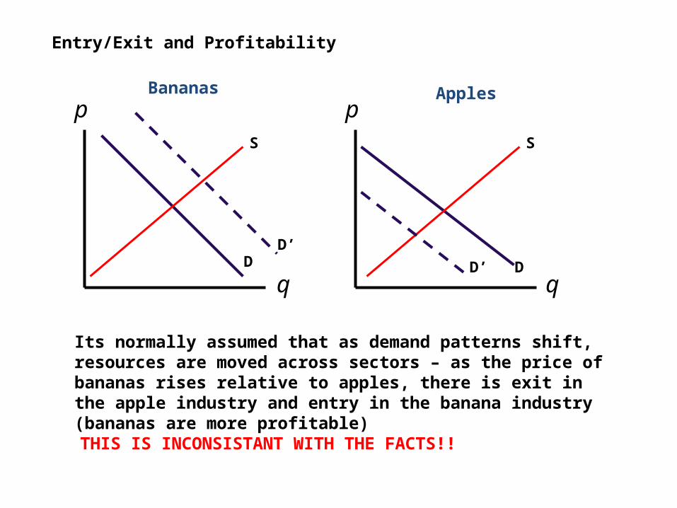
Entry/Exit and Profitability

p

D

p

q qD

SS

D’

D’

Its normally assumed that as demand patterns shift, resources are moved across sectors – as the price of bananas rises relative to apples, there is exit in the apple industry and entry in the banana industry (bananas are more profitable)

Bananas Apples

THIS IS INCONSISTANT WITH THE FACTS!!

Evolving Market Structures….Some Facts

Entry is common: Entry rates for industries in the US between 1963 – 1982 averaged 8-10% per year.

Entry occurs on a small scale: Entrants for industries in the US between 1963 – 1982 averaged 14% of the industry.

Survival Rates are Low: 61% of entrants will exit within 5 years. 79.6% exit within 10 years.

Entry is highly correlated with exit across industries: Industries with high entry rates also have high exit rates

Entry/Exit Rates vary considerably across industries: Clothing and Furniture have high entry/exit, chemical and petroleum have low entry/exit.

EntrantsMarket Dominated by Incumbents

Exits

The data suggests that most industries are like revolving doors – there is always a steady supply of new entrants trying to survive.

The key source of variation across industries is the rate of entry (which controls the rate of exit)

Is this a result of predatory practices by the incumbents?

Predatory Pricing vs. Profit Maximizing

Predatory pricing describes actions that are optimal only if they drive out rivals or discourage potential rivals!

2120120 qqP 40

20100 12

qq

Recall the previous example…each firm has a marginal cost of $20

11070 qP With limit pricing, firm 1 chooses a production level to drive price down to marginal cost

201070 1 qP 0

5

2

1

q

q

1q

2q

Firm 2Firm 1’s “entry deterring” output

Profit maximizing output

Entry deterrence generally involves overproducing today to drive your opponent out of business!

Firm 1

Overproduction by firm 1.

There have been numerous cases involving predatory pricing throughout history.

There are two good reasons why we would most likely not see predatory pricing in practice

1. It is difficult to make a credible threat (Remember the Chain Store Paradox)!

2. A merger is generally a dominant strategy!!

Standard Oil

American Sugar Refining Company

Mogul Steamship Company

Wall Mart

AT&T

Toyota

American Airlines

Capacity as a Commitment Device in Predatory Pricing

In 1945, the US Court of Appeals ruled that Alcoa was guilty of anti-competitive behavior. The case was predicated on the view that Alcoa had expanded capacity solely to keep out competition – Alcoa had expanded capacity eightfold from 1912 – 1934!!

In the 1970’s Safeway increased the number of stores in the Edmonton area from 25 to 34 in an effort to drive out new chains entering the area (It did work…the competition fell from 21 stores to 10)

In the 1970’s, there were 7 major firms in the titanium dioxide market (A whitener used in paint and plastics). Dupont held 34% of the market but had a proprietary production technique that generated less pollution. When stricter pollution controls were imposed, Dupont increased its market share to 60% while the rest of the industry stagnated.

The Bottom Line…

There have been numerous cases over the years alleging predatory pricing. However, from a practical standpoint we need to ask three questions:

1. Can predatory pricing be a rational strategy?

2. Can we distinguish predatory pricing from competitive pricing?

3. If we find evidence for predatory pricing, what do we do about it?

Price Fixing and Collusion

Prior to 1993, the record fine in the United States for price fixing was $2M. Recently, that record has been shattered!

Defendant Product Year Fine

F. Hoffman-Laroche Vitamins 1999 $500M

BASF Vitamins 1999 $225M

SGL Carbon Graphite Electrodes 1999 $135M

UCAR International Graphite Electrodes 1998 $110M

Archer Daniels Midland Lysine & Citric Acid 1997 $100M

Haarman & Reimer Citric Acid 1997 $50M

HeereMac Marine Construction 1998 $49M

In other words…Cartels happen!

01002003004005006007008009001000

1993 1994 1995 1996 1997 1998 1999

Antitrust Criminal Division Fines ($ Millions)

Cartel Formation

In a previous example, we had three firms, each with a marginal cost of $20 facing a market demand equal to

32120120 qqqP If we assume that these firms engage in Cournot competition, then we can calculate price, quantities, and profits

31$

45$

75.33

25.1

i

i

i

P

qQ

Mq

Firm Output

Industry Output

Market Price

Firm Profits

Total industry profit is $93

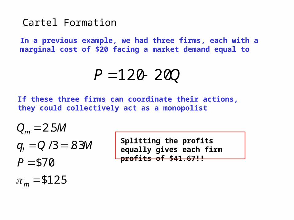
Cartel Formation

In a previous example, we had three firms, each with a marginal cost of $20 facing a market demand equal to

QP 20120 If these three firms can coordinate their actions, they could collectively act as a monopolist

125$

70$

83.3/

5.2

m

i

m

P

MQq

MQ

Splitting the profits equally gives each firm profits of $41.67!!

Cartel Formation

While it is clearly in each firm’s best interest to join the cartel, there are a couple problems:

With the high monopoly markup, each firm has the incentive to cheat and overproduce. If every firm cheats, the price falls and the cartel breaks down

Cartels are generally illegal which makes enforcement difficult!

Note that as the number of cartel members increases the benefits increase, but more members makes enforcement even more difficult!

Cartels - The Prisoner’s Dilemma

Jake

Clyde

Cooperate Cheat

Cooperate $20 $20 $10 $40

Cheat $40 $10 $15 $15

The problem facing the cartel members is a perfect example of the prisoner’s dilemma !

But we know that cartels do happen!!

Time0 1 2 3 4 5

Play Cournot Game

We can assume that cartel members are interacting repeatedly over time

Play Cournot Game

Play Cournot Game

Play Cournot Game

Play Cournot Game

Play Cournot Game

Cartel agreement made at time zero.

However, we’ve already shown that if there is a well defined endpoint in which the game ends, then the collusive strategy breaks down (threats are not credible)

Cartel members might cooperate now to avoid being punished later

Cooperation also occurs with an infinite horizon (i.e. the game never ends!!)

Time0 1 2 3 4 5

Play Cournot Game

Play Cournot Game

Play Cournot Game

Play Cournot Game

Play Cournot Game

Play Cournot Game

Cartel agreement made at time zero.

)()( CheatingPDVnCooperatioPDV

Firms will cooperate when its in their best interest to do so!

Cartels are easier to maintain when there are higher annual profits and interest rates are low!

Where is collusion most likely to occur?

High profit potential

The more profitable a cartel is, the more likely it is to be maintained

Inelastic Demand (Few close substitutes, Necessities)

Cartel members control most of the market

Entry Restrictions (Natural or Artificial)

Its common to see trade associations form as a way of keeping out competition (Florida Oranges, Got Milk!, etc)

April 15,1996 (“Grape Nut Monday”): Post Cereal, the third largest ready-to-eat cereal manufacturer announced a 20% cut in its cereal prices

Kellogg’s eventually cut their prices as well (after their market share fell from 35% to 32%)

The breakfast cereal industry had been a stable oligopoly for years….what happened?

Supermarket generic cereals created a more competitive pricing atmosphere

Changing consumer breakfast habits (bagels, muffins, etc)

Where is collusion most likely to occur?

Low cooperation costs

If it is relatively easy for member firms to coordinate their actions, the more likely it is to be maintained

Small Number of Firms with a high degree of market concentration

Similar production costs

Little product differentiation

Some cartels might require explicit side payments among member firms. This is difficult to do when cartels are illegal!

Detecting Collusion

In general, it is difficult to distinguish cartel behavior from regular competitive behavior (remember, the government does not know each firm’s costs, the nature of demand, etc)

Signs of Potential Collusion

Little relationship between price and costs

Little relationship between price and information sets

Excess Capacity (as a means of retaliation)