1

Economic integration in Latin America

By

Hem C. Basnet*

Department of Economics

South Illinois University Carbondale

Carbodale, IL 62901 Phone: 618-453-5061

E-mail: hcbasnet@siu.edu

And

Subhash C. Sharma

Department of Economics

South Illinois University Carbondale

Carbodale, IL 62901 Phone: 618-453-5082

E-mail: sharma@siu.edu

Working Paper

October, 2010

* Corresponding author

2

Economic integration in Latin America

Abstract

This study investigates the feasibility of economic integration in Latin America by considering

the seven largest economies in the region i.e. Argentina, Brazil, Chile, Colombia, Mexico, Peru

and Venezuela. We hypothesize that if the seven largest economies in the region are integrated

then the smaller economies will follow the suit. Towards this goal we analyze the long-term

and short-term relationship among key macro variables—real GDP, intra-regional trade, private

investment and consumption in these seven countries. We observe that all variables in these

countries are driven by more than one common trends and these variables also share common

cycles. The common trend-common cycle decomposition of real GDP, private investment and

consumption reveal that the economic fluctuations in these countries follow a similar pattern in

terms of duration, intensity and timing both in the long and the short run. Since these countries

demonstrate a high degree of co-movement among key macro variables these seven largest

countries in Latin America can lead the path of integration process in the region and reap the

benefits of economic integration.

Key words: common trends, common cycles, economic integration, common currency.

JEL Classification: E2, E3, E6.

3

Economic integration in Latin America

1. Introduction

Various countries over time realize that the socio-economic problems they are facing

cannot simply be coped with by individual efforts. As a result they begin to team up with

neighboring countries in the region, and this process is deepening now. The most obvious and

successful example is the European Union (EU)1 which has teamed up a number of isolated

countries to become a fully integrated economic unit. Regional integration is considered growth

enhancing. Integration necessarily implies free mobility of factors such capital, labor,

entrepreneurship, etc. among member countries. It will create a greater market in the region,

demolish the constraint of factor mobility and increase bargaining power in the global

economy.

Many countries around the world are trying to follow the integrationist footsteps of

Europe. The core lesson learned from European success is that despite many differences with

respect to goals, objectives and policies among countries in a region, economic integration

among those countries can take place and become successful. A greater degree of

macroeconomic synchronization or business cycles co-movements is regarded the key to

successful integration. A complete regional integration is materialized by having monetary

union with a single (optimum) currency in the region such as the European monetary union

with the Euro. Optimum currency areas are groups of regions with economies closely linked by

trade in goods and services and by factor mobility. A single currency will best serve the

economic interest of each of its members if the degree of output and factor trade among the

included economies is high (Krugman and Obsfeld, 2008). Rose and Wincoop(2001) note that

1 The EU was established by the Treaty of Maastricht on 1 November 1993 upon the foundations of the European

Economic Community. It consists of 27 member countries. They have had a common currency called Euro since

1999.

4

national money seems to be a significant barrier to international trade. Currency unions lower

these monetary barriers to trade and are thus associated with higher trade and welfare.

With the inception of World Trade Organization (WTO) many countries opened up

their economies and liberalized the trade policies. At the mean time, countries in different

regions began to form free trade agreements (FTAs)2 or preferential trade agreements (PTAs).

As a matter of fact, the first level of economic integration begins with such agreements. In light

of this new world order, Strydom (1995) writes a single country regardless of its economic,

military and cultural power or influence cannot stand alone in dealing with the many challenges

they face or might face. Individual countries have thus no choice but to adopt or implement

outward-oriented policies. Additionally, empirical evidence suggests that countries under

economic union or FTAs tend to trade three times more with each other than with non-member

countries (see Rose and Wincoop, 2001)

The existence of similar business fluctuations or business cycle synchronization is

considered a necessary condition for the harmonization of economic policies and institutions

among countries involved in an economic integration process (Christodoulakis, Dimelis and

Kollintzas, 1995; Fiorito and Kollintzas, 1994). The concept of interdependence of economies

is also known in the literature as macroeconomic interdependence which gives rise to economic

integration in any region. Macroeconomic interdependence is referred to as comovement

between real and monetary sectors between or among countries. If business cycle fluctuations

are synchronized, harmonized policies to cope with the cycles across countries can be effective

(Sato and Zhang 2006). Additionally, macroeconomic interdependence has been crucial for the

integration of financial markets as well (see Sharma and Wongbangpo, 2002).

2 FTAs eliminate import tariffs as well as import quotas between signatory countries.

5

The presence of strong macroeconomic synchronization is regarded as a rationale for

creation of Regional Trade Agreements (RTAs). The concept of RTAs in Latin American

context dates back to 1960 when the Latin American Free Trade Association (LAFTA)3 was

created. The goal of LAFTA was to create a common market in Latin America and it was

perceived as a first step to economic integration in Latin America. Many Latin American

economists took it as a promising vehicle for enhancing economic and social development in

their respective countries (Rosenthal, 1985). But, the initial enthusiasm gradually faded away

and a general air of pessimism regarding integration spread. Over the course of the past three

and half decades, the process of economic integration has suffered numerous setbacks.

Frequent abrupt political changes have been a deterrent to economic cooperation. During the

1960s, LAFTA was disrupted by military coups in Argentina and Brazil (Ffrench-Davis,1989).

Due to this, we believe, integration movement could not make any progress and obviously

could not reap the benefits of greater extension in the region. In addition to that the Latin

American countries were left out of this line of research mainly for lack of stability and lack of

data (Fullerton and Araki, 1996, Mena, 1995). However, the movement toward Latin American

economic integration is gaining momentum. The formulation of the Common Market of the

south or MERCOSUR—a largest regional trade area signed in 1991 between Argentina,

Brazil, Paraguay, Uruguay (and more recently Venezuela), with Bolivia, Chili, Peru, Colombia,

and Ecuador as associates—is taken as momentum gain. As a matter of fact, more than 14

agreements—free trade areas or custom unions—since 1990 have been made in the region.

Hence, with this renewed interest this is of extraordinary relevance to investigate

macroeconomic interdependence for Latin American countries.

3 The initial signatories in LAFTA charter were Argentine, Brazil, Chile, Mexico, Paraguay, Peru, and Uruguay.

By 1970, LAFTA expanded to include four more Latin American nations—Bolivia, Colombia, Ecuador and

Venezuela. In 1980, LAFTA reorganized into the Latin American Integration Association (ALADI). There are

currently at least seven active RTAs in Latin America. i) the southern common market (Mercosur) ii) Andean

community of nations iii) Central American integration system (CA4), iv) The Caribbean Free Trade Association

(CARIFTA), v) Union of South American Nations, vi) Free trade area of the Americas (FTAA), and vii) G3

6

The decade of the 1990s was characterized by an intense parley of regional trade

agreement in Latin America. More than 14 agreements4--free trade areas or custom unions—

since 1990 have been made in the region. However, Latin America seems to be far behind in its

endeavor to formulate regional integration and enjoy the benefits of greater integration. What

are the main hurdles that have suppressed all the initiatives that have emerged so far? Or how

feasible it is to imitate the European style integration model in Latin America? This study

analyzes the feasibility of economic integration in Latin America. According to conventional

literature a set of countries involved in integration should meet certain preconditions such as

business cycle synchronization, a strong similarity in the adjustment process and the

convergence of policy responses. The aim of this research is twofold: to explore the degree of

macroeconomic synchronization of Latin American economies and hence the feasibility of

economic integration. We aim to achieve this goal by analyzing the intra-Latin America trade

and business cycle synchronization (common cycle/trend) among key macroeconomic

variables. The macro-variables chosen are: gross domestic product, trade flows, private

consumption and investment. According to Mundell (1961) the overall degree of economic

integration can be judged by looking at the integration of product markets, that is the extent of

trade between the joining country and the currency area, and at the integration of factor

markets, that is, the ease with which labor and capital can migrate between the joining country

and the currency area. In this study, real GDP and intra-regional trade captures the integration

of product markets and private investment represents the factor market (i.e. capital).

Additionally, we further investigate the short-run and long run behavior of consumption in

these countries. Hence, selection of our variables for this study is relevant and justifiable.

We have chosen the seven largest economies (Argentina, Brazil, Chile, Colombia,

Mexico, Peru, and Venezuela) from Latin America. Together, these seven countries out of 21

4 For details see: Allegret and Sand-Zantman (2009)

7

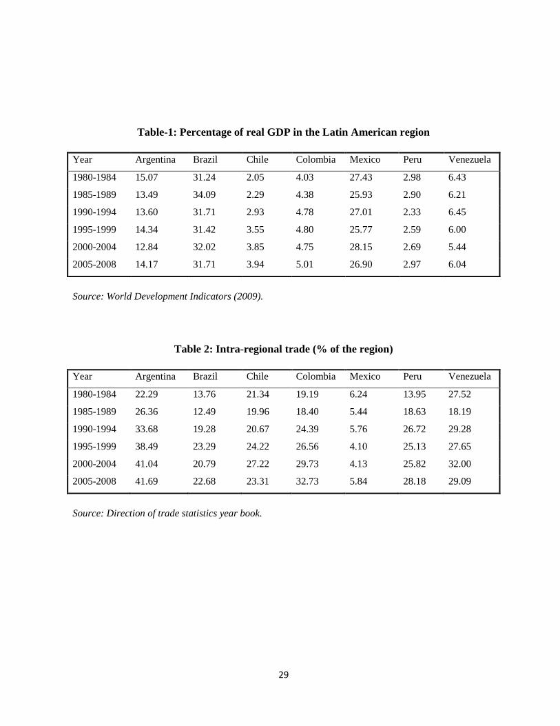
Latin American countries account for more than 90 percent of the continent’s GDP and about

93 Percent of its population in 2008. More importantly, these seven countries’ real GDP always

maintain more than 89% of their five year averages in the region from 1980-2008 (see table 1).

Similarly, their trade share in the region is also significant and growing (see table 2). Argentina

has a higher trade share in the region during 1980-2008. On five years average its exports plus

imports for the region almost doubled the last decade from its eighties share. Mexico, being the

second largest economy after Brazil, has the smallest regional trade share (see table 2).

Obviously, Mexico trades more with its northern partners—USA and Canada. The rest of the

countries in this study have an average of about one fourth of the trade share in the region.

Therefore, these countries are leading economies in the region and we believe that the possible

integration of these leading seven countries would bring the other countries in. Our rationale

for this choice is that if macro variables in the leading economies are synchronized then the

smaller economies will catch up with them, which will result in a complete integration in the

entire continent.

Unlike the case of European integration, sufficient amount of empirical studies have not

been devoted for the case of Latin America, only marginal attention has been paid to in this

regard. Hence, this study will have great policy implication in context of economic integration

in Latin America. Past studies have examined economic integration based on the observed

similarities of the economies and the correlation analysis of the business cycles. The problem

with these methodologies is that the degree of correlation between shocks does not accurately

follow short-run output co-movements. Hence, we complement our analysis by both testing

cointegration (to assess the existence of long-run movements in real output among countries)

and for the existence of common short-run cycles as suggested by Vahid and Engle (1993).

Sharing similar short and long run macro trends necessitates few or no country-specific policies

that may hinder the stability of the union (Abu-Aarn and Abu-Bader, 2008). For an integration

8

process to be viable, it is essential to have both long-run synchronous real output co-

movements and short-run common business cycles to minimize the need for country-specific

policies that may hinder the stability of the union. To the best of our knowledge, very few

studies, most notably Engle and Issler (1993), have investigated the common trends and

common cycles in three Latin American economies. We contribute to these efforts by exploring

long run trends and short run cycles among key macro variables of the seven largest Latin

American economies.

The chief policy implication of this research is concerning monetary union for Latin

American countries. Monetary union is the final stage of economic integration. The

preconditions for economic integration are also applicable to monetary union. More simply, if

these countries follow the long term trends and also the short term business cycles then they

can implement a single monetary policy and currency for the integrated region. Therefore, the

study Macroeconomic synchronization is crucial for the success of integration. The argument

behind this logic is that if the impact of a shock across countries is not symmetric then

harmonized monetary and fiscal policies could be detrimental.

The rest of the paper is organized as follows. The next section presents a review of past

studies that deal with the topic of common movement between macroeconomic time series and

economic integration. Section 3 describes the methodology used to analyze business cycle

synchronization and integration. In section 4, the empirical results are reported and commented

on. Finally, we state concluding remarks.

2. Literature Review

The business cycles co-movements between the economies of Latin American countries

have been examined from a variety of perspectives. For instance, Engle and Issler (1993)

investigated the degree of short and long run comovement in GDP-per capita of three Latin

9

American countries (Argentina, Brazil and Mexico) using common trends and common cycles

methodology and document that while Argentine and Brazil share both long and short run co-

movement, Mexico does not have similar trend and cyclical behavior with any of those

countries. Similarly, Arnaudo and Jacobo (1997) considered the four Latin American

countries—Argentina, Brazil, Paraguay and Uruguay—and noted that there is significant

synchronization only between Argentina and Brazil. Jacobo (2002) studied macroeconomic

behavior of five Latin American countries for period the 1970-1997 and finds that the group of

these countries did not have a strong economic linkage. More interestingly, in a study of 8

Latin American countries and the United States Mejia-Reyes (1999) also found no evidence of

a Latin American Common cycle but the author found significant synchronization between

several countries5 in bivariate context. Fiess (2007) measured the degree of business cycle

synchronization between Central America6 and the United States observed that business cycle

synchronization within Central American countries is quite low. This finding does not support

any macroeconomic coordination within Central America. In a recently published paper

Allegret and Sand-Zantman (2009) studied the feasibility of a Monetary Union between five

Latin American Countries—Argentina, Brazil, Chile, Mexico and Uruguay. In doing so, they

have investigated whether this set of countries is characterized by business cycle

synchronization. Based on results obtained from the Vector Auto Regression (VAR) model

these authors do not support monetary union in Latin American even though Uruguayan

economic activity depends mainly on Argentina and Brazilian business cycles.

5 Argentina – Brazil, Argentina – Peru, Bolivia – Venezuela, Brazil- Peru, Chile- United States, Argentina-

Bolivia, Mexico- Venezuela and Brazil-United States).

6 Costa Rica, El Salvador, Guatemala, Honduras, Nicaragua, Panama.

10

After inception of NAFTA7 several studies have examined the business cycle

synchronization particularly between US and Mexican economies and found the existence of

statistically significant common movements between two economies since then (Hernandez,

2004). This result is consistent with studies that examine economic interactions in a wide

sample of counties. For example, Anderson and Kwark (1999) reported a significant

relationship between trade openness and the synchronization of economic cycles in a set of 37

countries across the world.

Many have examined to what extent business cycles of the different countries are

similar8. In a recent paper, Adom, Sharma and Morshed (2010) examine the feasibility of

African economic integration by applying common trends and common cycles methodologies.

They find the presence of macroeconomic interdependence among eight largest African

economies and hence their results suggest that some preconditions for a successful integration

of Africa are currently in place. Haan and Montoya (2008) investigate regional business cycle

synchronization in the Euro area and found the Euro area has become more synchronized since

integration. This result, according to the authors has been able to dismiss the well-known

critique that a common monetary policy may not be good for all countries or regions in the

union (i.e. one size does not fit all).

In the race of regional integration, the Gulf Cooperation Council (GCC) is ahead of any

other region in the world. The GCC member countries have adopted the EU convergence

criteria9 and fulfillment of most of the convergence criteria has been achieved. Given the

7 North American Free Trade Area (NAFTA) which consists of US, Canada and Mexico.

8 e.g. Capannelli, Lee and Petri (2010), Rana (2007), McAdam (2007), Anderson and Moazzami (2003), Sharma

and Horvath(1997).

9 According to the article 121(1) of the European community treaty, the applicant countries should not exceed on

average 1.5% of inflation and 2% of nominal interest rates. Similarly, budget deficit and public debt to GDP ratio

should exceed more than 3% and 60% respectively. The last criterion is that applicant countries should not have

devalued its currency at least 2 years prior to joining EU.

11

preparation Abu-Aarn and Abu-Bader(2008) examine whether GCC countries are ready to

form a viable monetary union in the region. By studying long run trends and short run cycles on

their macro variables their findings do support for the readiness of the GCC countries to

establish a viable currency union. In contrary to this, Darrat and Al-Shamsi(2005) find

supportive evidence for the economic integration in the Gulf region. Selover (1999) studies co-

movements of business cycles between Indonesia, Malaysia, Philippines, Singapore, and

Thailand and their major trading partners the United States, Australia, Japan, and the European

Union and found the evidence of strong co-movement in these countries.

On multivariate trend-cycle decomposition, Vasta and Sharma (2010) investigate the

financial integration in ASEAN- 4 countries ( Malaysian, Philippine, Singapore and Thailand)

by looking at the short-run and long-run behavior of exchange rate series of these countries.

The authors conclude that the exchange rates of share long term trends and short term cycles.

3. Data and Methodology

We use yearly data on Real gross domestic product (RGDP), Intra-regional trade

(TRADE), Investment (INVEST) and Consumption (CONS) for the seven largest Latin

American countries—Argentina, Brazil, Chile, Colombia, Mexico, Peru and Venezuela. Data is

obtained from the World Development Indicators (WDI-2009) and various issues of the

Direction of Trade Statistics year book. Since we are investigating the feasibility of economic

integration in Latin America it makes a lot sense to investigate trade intensity among the

sample countries within the region. So we decided to use intra-regional trade data rather than

just trade flows measured by the sum of imports and exports. The intra-regional trade only

covers the sum of exports plus imports from countries under consideration into the Latin

American region. The time span for intra-trade ranges from 1978 to 2008 whereas for the rest

of the variables it ranges from 1960 to 2008. All data are in constant 2000 US dollar. In

12

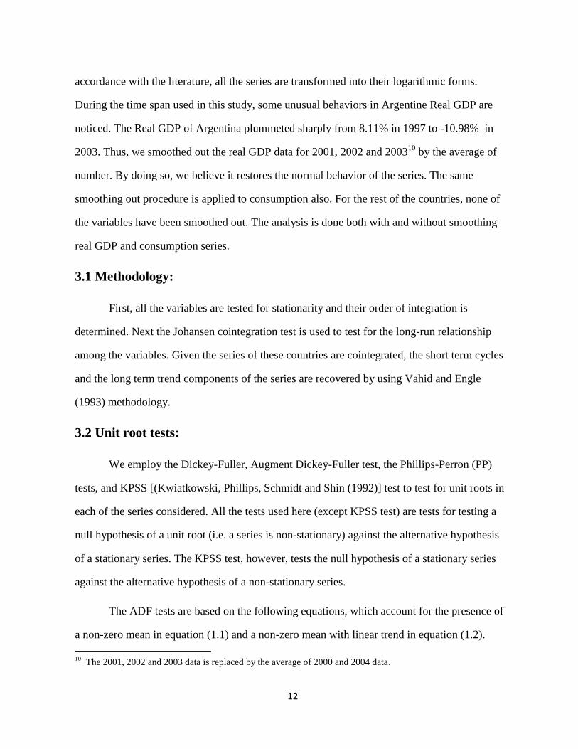
accordance with the literature, all the series are transformed into their logarithmic forms.

During the time span used in this study, some unusual behaviors in Argentine Real GDP are

noticed. The Real GDP of Argentina plummeted sharply from 8.11% in 1997 to -10.98% in

2003. Thus, we smoothed out the real GDP data for 2001, 2002 and 200310

by the average of

number. By doing so, we believe it restores the normal behavior of the series. The same

smoothing out procedure is applied to consumption also. For the rest of the countries, none of

the variables have been smoothed out. The analysis is done both with and without smoothing

real GDP and consumption series.

3.1 Methodology:

First, all the variables are tested for stationarity and their order of integration is

determined. Next the Johansen cointegration test is used to test for the long-run relationship

among the variables. Given the series of these countries are cointegrated, the short term cycles

and the long term trend components of the series are recovered by using Vahid and Engle

(1993) methodology.

3.2 Unit root tests:

We employ the Dickey-Fuller, Augment Dickey-Fuller test, the Phillips-Perron (PP)

tests, and KPSS [(Kwiatkowski, Phillips, Schmidt and Shin (1992)] test to test for unit roots in

each of the series considered. All the tests used here (except KPSS test) are tests for testing a

null hypothesis of a unit root (i.e. a series is non-stationary) against the alternative hypothesis

of a stationary series. The KPSS test, however, tests the null hypothesis of a stationary series

against the alternative hypothesis of a non-stationary series.

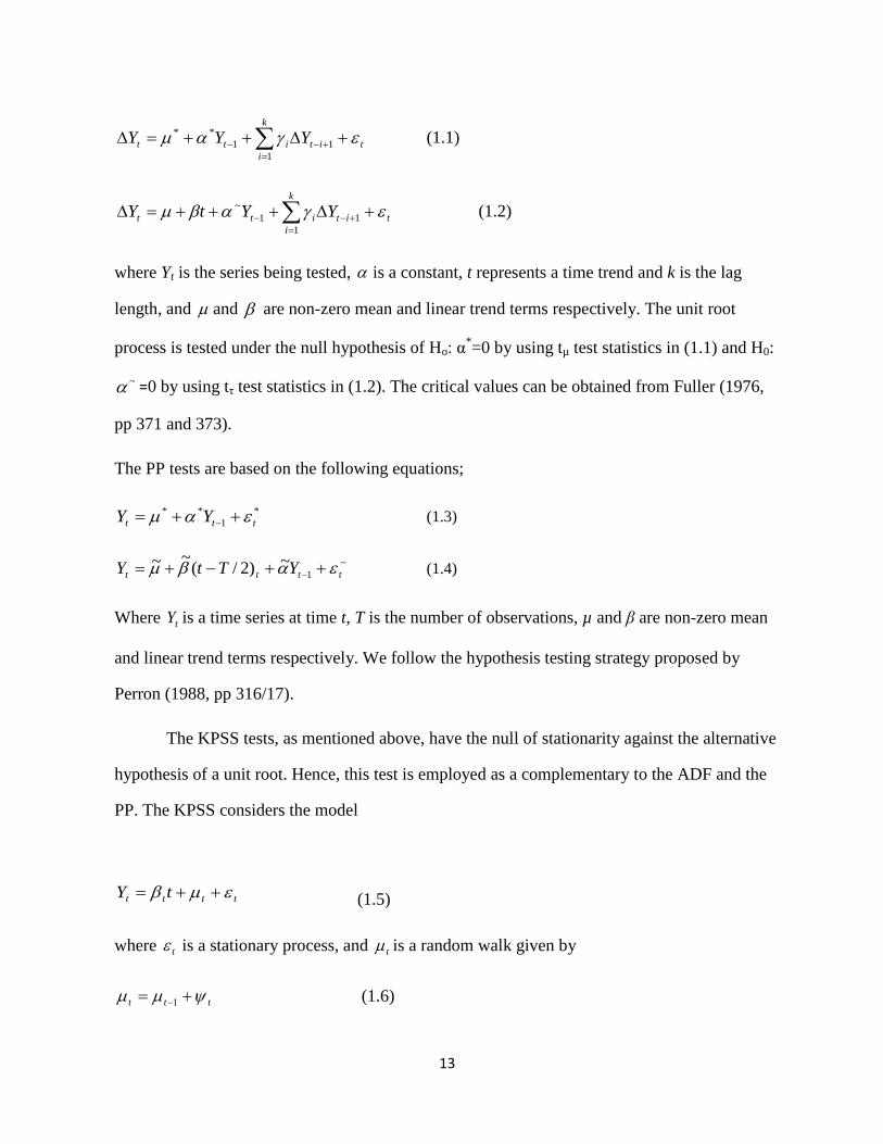
The ADF tests are based on the following equations, which account for the presence of

a non-zero mean in equation (1.1) and a non-zero mean with linear trend in equation (1.2).

10

The 2001, 2002 and 2003 data is replaced by the average of 2000 and 2004 data.

13

tit

k

i

itt YYY

1

1

1

** (1.1)

tit

k

i

itt YYtY

1

1

1

~ (1.2)

where Yt is the series being tested, is a constant, t represents a time trend and k is the lag

length, and and are non-zero mean and linear trend terms respectively. The unit root

process is tested under the null hypothesis of Ho: α*=0 by using tµ test statistics in (1.1) and H0:

~ =0 by using tτ test statistics in (1.2). The critical values can be obtained from Fuller (1976,

pp 371 and 373).

The PP tests are based on the following equations;

*

1

**

ttt YY (1.3)

~

1~)2/(

~~tttt YTtY (1.4)

Where tY is a time series at time t, T is the number of observations, µ and β are non-zero mean

and linear trend terms respectively. We follow the hypothesis testing strategy proposed by

Perron (1988, pp 316/17).

The KPSS tests, as mentioned above, have the null of stationarity against the alternative

hypothesis of a unit root. Hence, this test is employed as a complementary to the ADF and the

PP. The KPSS considers the model

(1.5)

where t is a stationary process, and t is a random walk given by

ttt 1 (1.6)

tttt tY

14

Their null hypothesis of stationarity is given by H0: σ2 =0 or t is a constant. This test

is based on the principle of a Lagrange Multiplier score test and the test statistics and the

critical values are provided by Kwaiatkowski et.al (1992).

3.3 Common Trend and Common Cycle analyses

3.3.1 Cointegration test:

We employ the maximum likelihood cointegration approach introduced by Johansen

(1988). The cointegration test begins by expressing series in (nx1) vector form.

Let Ven

t

Per

t

Mex

t

Col

t

Chl

t

Brl

t

Arg

t yyyyyyy ,,,,,, be a (7x1) vector of either GDPs or intra-

regional trade or investment or consumption of the seven countries under investigation. Thus,

the unrestricted Vector Auto regression (VAR) can be written as follows:

tptntt yAyAy ...11 (1.7)

where t is a vector of white noise residuals and p is the lag length. Following Johansen (1988)

and Johansen and Juselius (1990) the vector error correction model of the above equation (1)

can be rewritten in its first difference form:

ttptpttt yyyyy 1112211 ... (1.8)

where 1 ttt yyy

1

1

p

i

ii A ,

p

i

iA1

where is a (7x7) identity matrix and the term 1 ty contains information concerning long-run

relationship between the variables. Johansen (1988) notes that the number of cointegrating

vectors can be determined by the rank of matrix, r. If the matrix is of rank 0<r<7, then it

15

can be decomposed into , where )7(rx is the matrix of the cointegration coefficients

and )7(rx is the adjustment coefficients to the long run equilibrium. Given a (7 x1) vector yt if

there exists r < 7 linearly independent cointegrating vectors then it implies that there are (7-r)

common trends. The maximum likelihood based λtrace and λmax test statistics are used to identify

the number of independent cointegrating vectors. To test the null hypothesis r = 0 against the

alternative hypothesis r = 1,2, 3…7, λtrace is used whereas λmax tests the null r = 0 against the

alternative hypothesis that there are (r +1) cointegrating vectors.

3.3.2 Common cycles:

To test common cycles in the presence of common trends, we employ the methodology

purposed by Vahid and Engle (1993). According to Vahid and Engle (1993), this methodology

tests the significance of the connonical correlations between ty and

),...,,,( 1211 ptttt yyyyW . They point out that given r linearly independent

cointegrating vectors, if a series yt has common cycles there can, at most exist s = (n- r)

cofeature vectors that eliminate common cycles (see Vahid and Engle 1993, pp. 345). With s

number of cofeature vectors there exists (n-s) number of common cycles in a series. The test

statistic proposed by Vahid and Engle (1993) is

C(p*, s) = -(T-p*-1) )1ln( 2 i ~χ2 (1.9)

with (np*s + rs – ns + s2) degree of freedom, where 2

i are the s smallest squared canonical

correlations between ty and W, T is the number of observations, p* is the lag length of VAR

system in difference, and r represents the number of cointegrating vectors. Note that the test

statistic is for the null hypothesis that the dimension of the cofeature space is at least s. If there

exist s independent cofeature vectors then there are (n-s) common cycles. A dimension of (nxs)

16

matrix ~ and of (nxr) matrix are referred to as the cofeature and cointegrating vectors

respectively. In a case when r+s = n, Vahid and Engle (1993) decompose the permanent

(trend) and the transitory (cycle) components of each series. In this case (i.e r+s = n ) there will

be an (nxn) matrix A=

~ with full rank and hence it will have 1A . We can proceed trend

and cycle decomposition by partioning the columns of 1A such as |~1A . Finally

we recover the trend and cyclical components in the following way:

tttt yyyAAy ~~1 (1.10)

= Trend components + Cycle components

Equation (1.10) is used to decompose a trend-cycle in a series. The first term represents only

the trend part since ty ~ is a random walk and is free from any cycles. The second part is

characterized by cyclical components as ty is serially correlated and I(0).

4. Empirical Results:

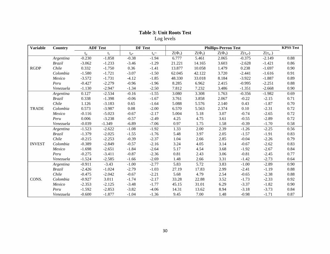
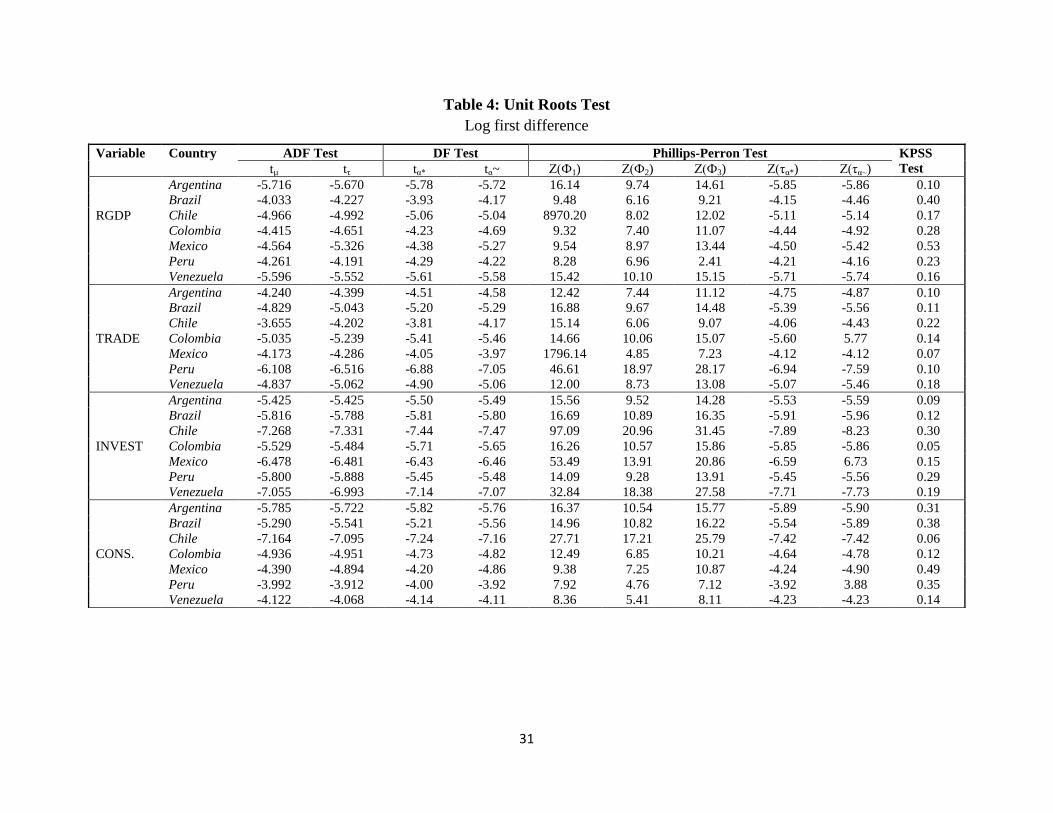
The results of the unit root tests are reported in table 3 and 4. The test statistics show

that a null hypothesis of unit roots cannot be rejected in their levels whereas the unit roots of

the first difference reject the null at 5% significance level. These results suggest that series are

first-difference stationary. The sequential likelihood ratio tests suggest the optimal lag length

for the cointegration test to be one for real GDP and intra-trade and two for investment and

consumption.

17

4.1 Common Trend Analysis

We consider the following model for each of the series investigated i.e.

Ven

t

Per

t

Mex

t

Col

t

Chl

t

Brl

t

Arg

tt yyyyyyyy ,,,,,,

where, yt is a (7 x1) vector of real GDP or intra-regional trade or investment or consumption of

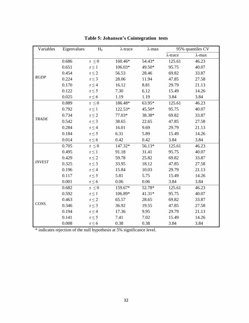
seven Latin American countries. The results for the cointegration tests are presented in table 5

Both λtrade and λmax ensure the presence of two cointegrating vectors (i.e. r =2) in real GDP.

This means that there exists 5 common trends in the real GDP of these seven countries. The

existence of common trends indicates that the real GDP of these countries move together in the

long run. Similarly, we cannot reject the null of at most three cointegrating vectors, and

conclude that there exists 3 cointegrating vectors (i.e. r=3). This implies the existence of 4

common stochastic trends in trade variables. In fact, the existence of at least one cointegrating

vector is required to establish a long run relationship among a set of variables. Thus, this result

suggests that trade among these countries cannot swing for long time, they eventually move

together. This can be clearly viewed from the five years average data on intra-regional trade of

these countries. Table 2 tabulates data on export plus import of these countries in the region.

Mexico’s trade share is very low vis- à –vis the rest of the countries. Its close tie with North

American Free Trade Agreement (NAFTA) members (USA and Canada) can be attributed to

the low share. Cointegration results reveal that both investment and consumption also share 6

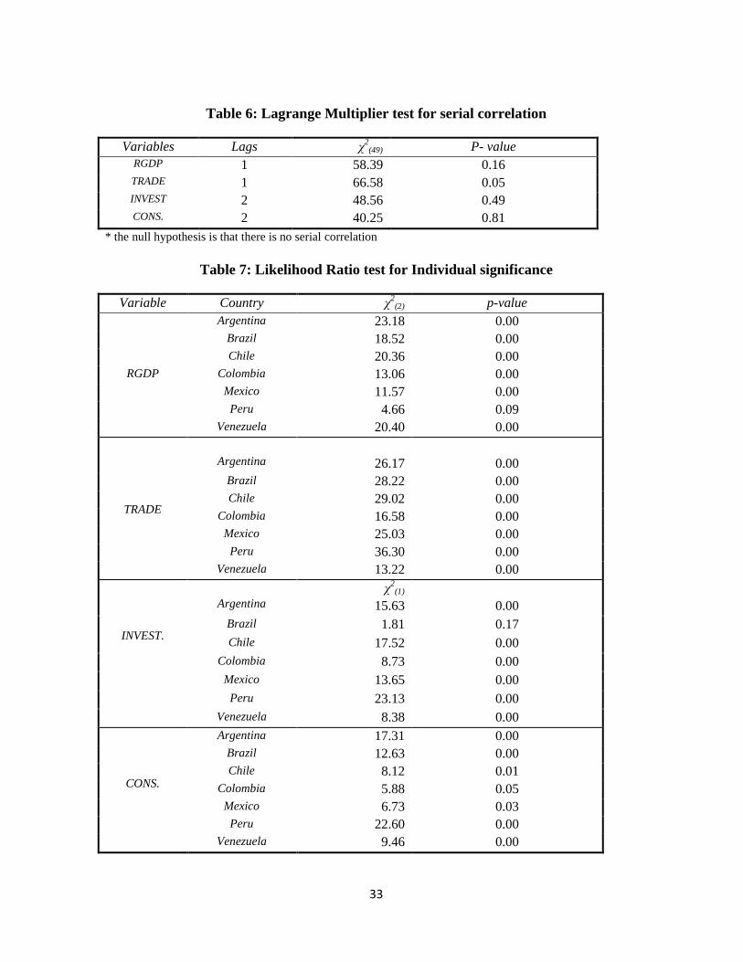
and 5 common trends in the long-run respectively. We also check whether the residuals of the

four variables are serially correlated. The Lagrange Multiplier Autocorrelation test reported in

table 6 reveal that we accept the null hypothesis of no serial correlation at 5% significance level

in each cointegrating model.

While the presence of one or more cointegrating vectors necessitates the long

relationship among them, each variable in the model may not be statistically significant to

18

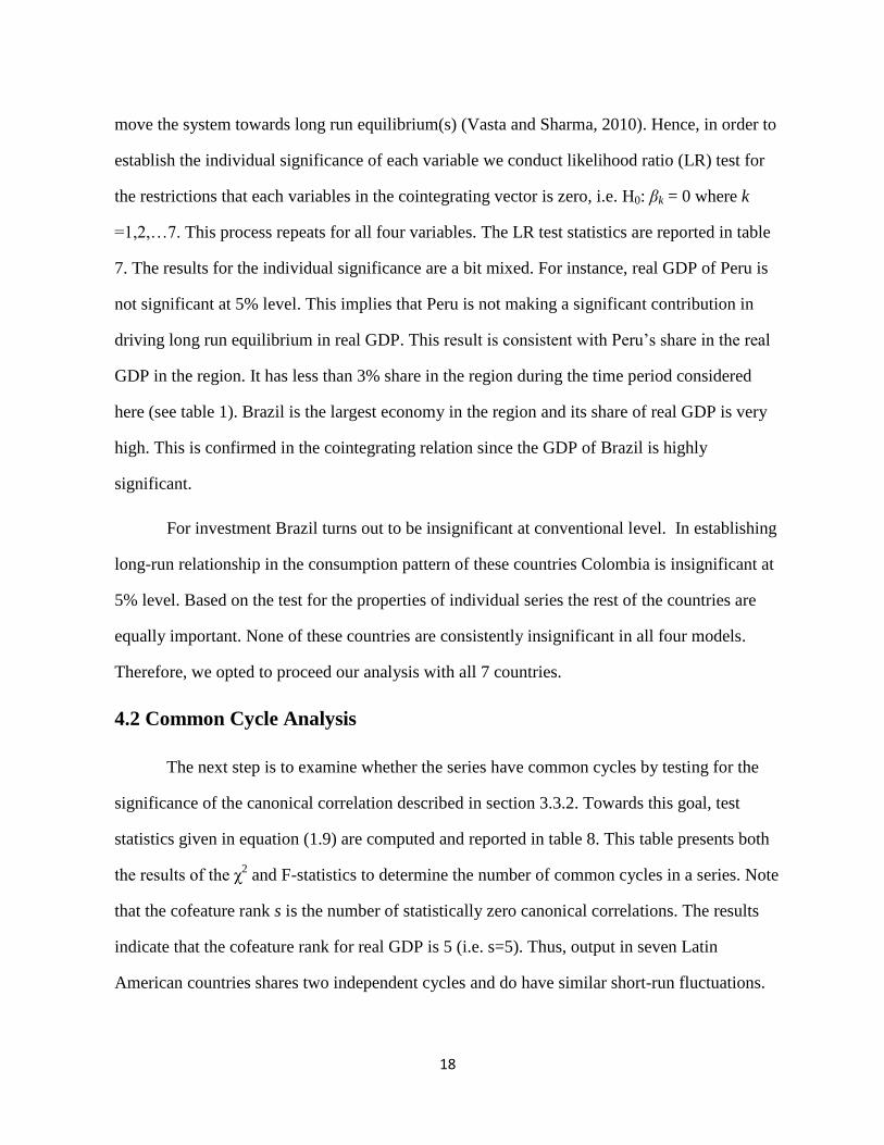
move the system towards long run equilibrium(s) (Vasta and Sharma, 2010). Hence, in order to

establish the individual significance of each variable we conduct likelihood ratio (LR) test for

the restrictions that each variables in the cointegrating vector is zero, i.e. H0: βk = 0 where k

=1,2,…7. This process repeats for all four variables. The LR test statistics are reported in table

7. The results for the individual significance are a bit mixed. For instance, real GDP of Peru is

not significant at 5% level. This implies that Peru is not making a significant contribution in

driving long run equilibrium in real GDP. This result is consistent with Peru’s share in the real

GDP in the region. It has less than 3% share in the region during the time period considered

here (see table 1). Brazil is the largest economy in the region and its share of real GDP is very

high. This is confirmed in the cointegrating relation since the GDP of Brazil is highly

significant.

For investment Brazil turns out to be insignificant at conventional level. In establishing

long-run relationship in the consumption pattern of these countries Colombia is insignificant at

5% level. Based on the test for the properties of individual series the rest of the countries are

equally important. None of these countries are consistently insignificant in all four models.

Therefore, we opted to proceed our analysis with all 7 countries.

4.2 Common Cycle Analysis

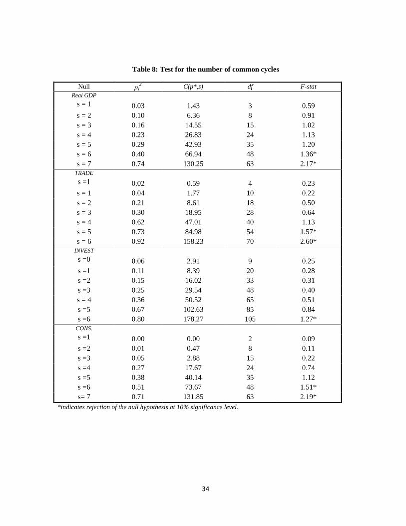
The next step is to examine whether the series have common cycles by testing for the

significance of the canonical correlation described in section 3.3.2. Towards this goal, test

statistics given in equation (1.9) are computed and reported in table 8. This table presents both

the results of the χ2 and F-statistics to determine the number of common cycles in a series. Note

that the cofeature rank s is the number of statistically zero canonical correlations. The results

indicate that the cofeature rank for real GDP is 5 (i.e. s=5). Thus, output in seven Latin

American countries shares two independent cycles and do have similar short-run fluctuations.

19

In this case we have r+s=n (i.e. 2+5=7) which allows us to do a special trend-cycle

decomposition.

The null hypothesis that the cofeature space has a dimension of seven is rejected for the

rest of three variables—trade, investment and consumption. The cofeature rank for trade is 5

(i.e. s = 5). This implies that these seven countries share two common cycles in their trade

pattern. We further note that for investment s = 6, suggesting at least one common cycle.

Finally, at conventional significance level both χ2 and F-test confirm that for consumption s=5.

This suggests that the system of seven Latin American consumption series possesses two

common cycles. In this study the special condition i.e. r+s =n is not satisfied for trade variable.

However, for investment and consumption the number of cointegrating vectors (r) and

cofeature vectors (s) add up to the number of the total variable (n). Therefore, we can

decompose three out of four variables into their trend and cyclical components.

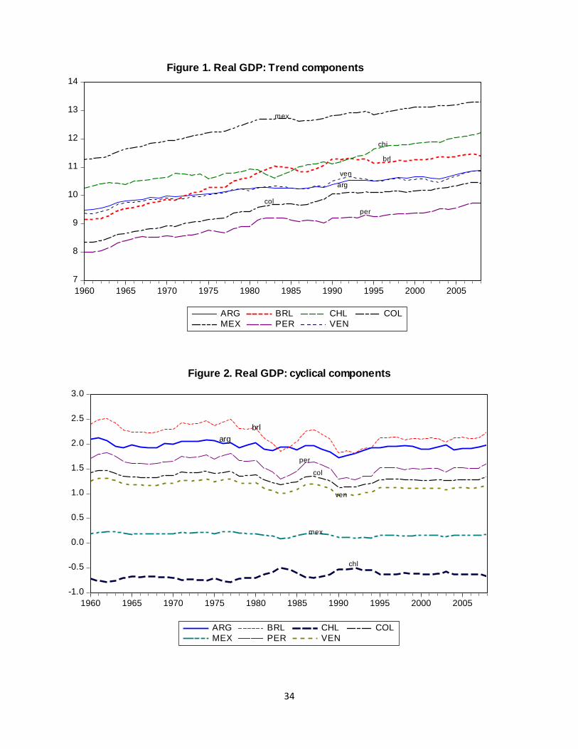
GDP: A plot of the trends and cycles of real GDP is given in figures 1 and 2. From the

figures, it is so apparent that the long term trends and short term cycles are synchronized. The

long-run co-movement of real GDP in seven Latin American economies suggests that these

countries are reacting to the shocks in a similar way. We can also observe two noticeable

characteristics in their trend components. First, Argentine and Venezuelan trend components

are highly synchronized throughout the sample period. Second, the economic prosperity in

Brazil is coincided by economic slump in Chile and vice versa during 1981 to 1992. The

existence of no independent trend can also be viewed by the band these countries are holding.

The constant gap in their long run co-movement further implies that although these economies

might have policy differences (monetary and fiscal) they are not creating any substantial output

differences. Furthermore, the divergence from the long run equilibrium is short-lived and real

GDP of these economies adjusts to the long run common trend.

20

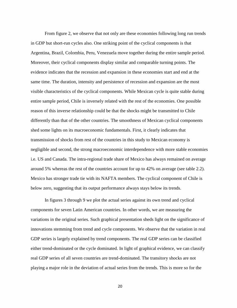
From figure 2, we observe that not only are these economies following long run trends

in GDP but short-run cycles also. One striking point of the cyclical components is that

Argentina, Brazil, Colombia, Peru, Venezuela move together during the entire sample period.

Moreover, their cyclical components display similar and comparable turning points. The

evidence indicates that the recession and expansion in these economies start and end at the

same time. The duration, intensity and persistence of recession and expansion are the most

visible characteristics of the cyclical components. While Mexican cycle is quite stable during

entire sample period, Chile is inversely related with the rest of the economies. One possible

reason of this inverse relationship could be that the shocks might be transmitted to Chile

differently than that of the other countries. The smoothness of Mexican cyclical components

shed some lights on its macroeconomic fundamentals. First, it clearly indicates that

transmission of shocks from rest of the countries in this study to Mexican economy is

negligible and second, the strong macroeconomic interdependence with more stable economies

i.e. US and Canada. The intra-regional trade share of Mexico has always remained on average

around 5% whereas the rest of the countries account for up to 42% on average (see table 2.2).

Mexico has stronger trade tie with its NAFTA members. The cyclical component of Chile is

below zero, suggesting that its output performance always stays below its trends.

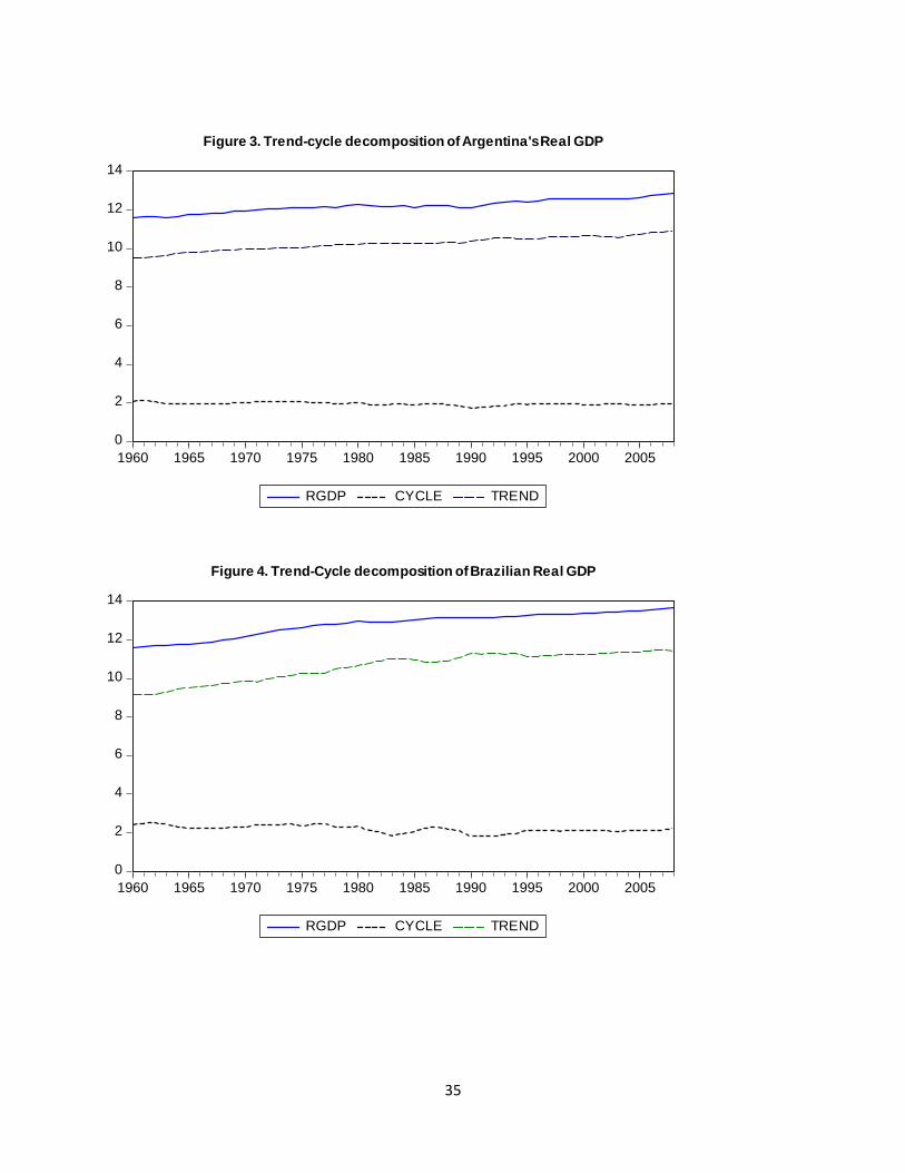
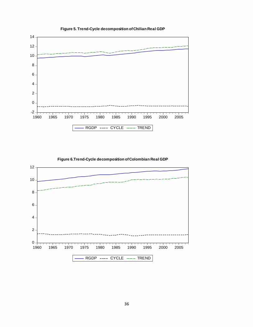
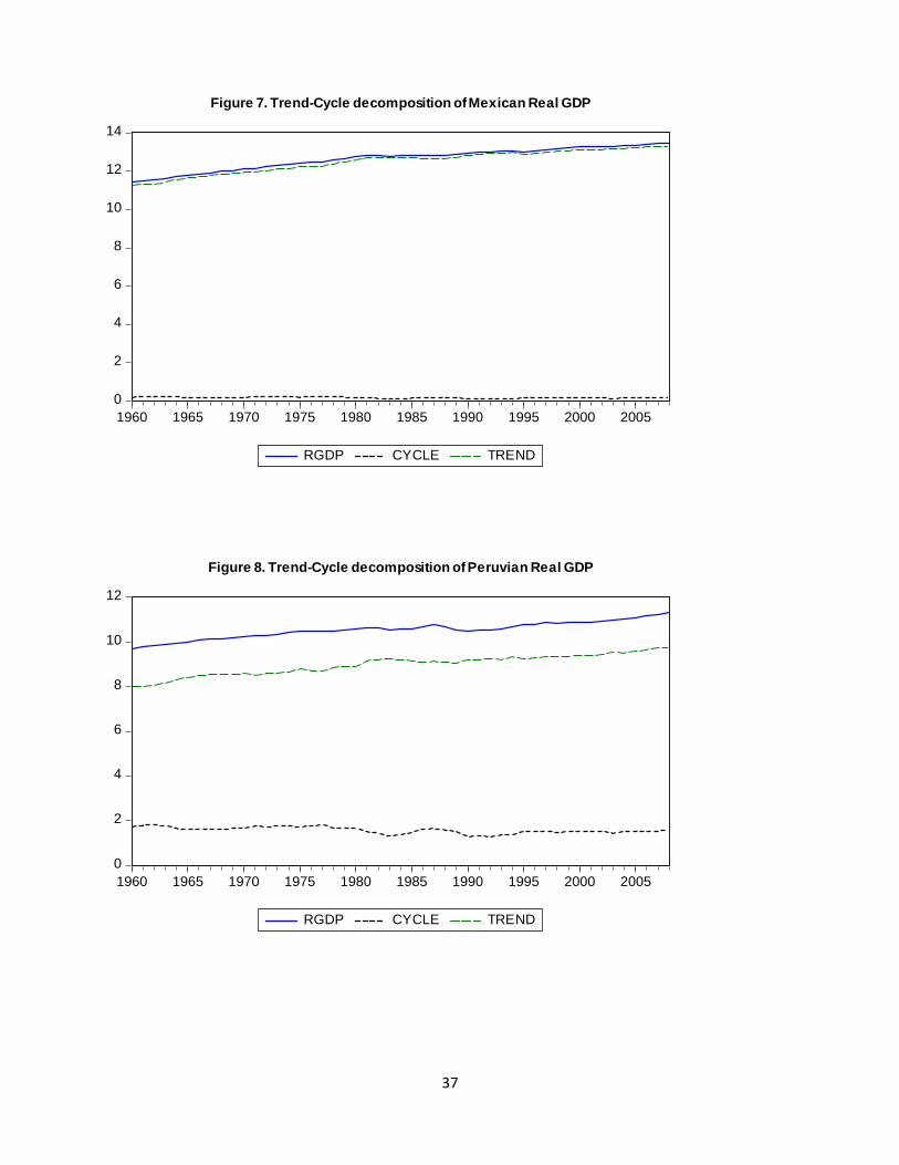
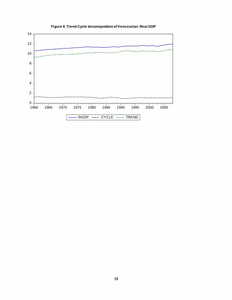
In figures 3 through 9 we plot the actual series against its own trend and cyclical

components for seven Latin American countries. In other words, we are measuring the

variations in the original series. Such graphical presentation sheds light on the significance of

innovations stemming from trend and cycle components. We observe that the variation in real

GDP series is largely explained by trend components. The real GDP series can be classified

either trend-dominated or the cycle dominated. In light of graphical evidence, we can classify

real GDP series of all seven countries are trend-dominated. The transitory shocks are not

playing a major role in the deviation of actual series from the trends. This is more so for the

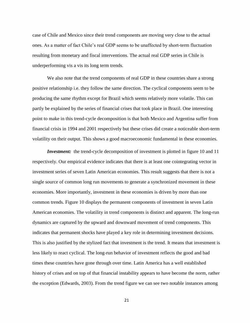
21

case of Chile and Mexico since their trend components are moving very close to the actual

ones. As a matter of fact Chile’s real GDP seems to be unaffected by short-term fluctuation

resulting from monetary and fiscal interventions. The actual real GDP series in Chile is

underperforming vis a vis its long term trends.

We also note that the trend components of real GDP in these countries share a strong

positive relationship i.e. they follow the same direction. The cyclical components seem to be

producing the same rhythm except for Brazil which seems relatively more volatile. This can

partly be explained by the series of financial crises that took place in Brazil. One interesting

point to make in this trend-cycle decomposition is that both Mexico and Argentina suffer from

financial crisis in 1994 and 2001 respectively but these crises did create a noticeable short-term

volatility on their output. This shows a good macroeconomic fundamental in these economies.

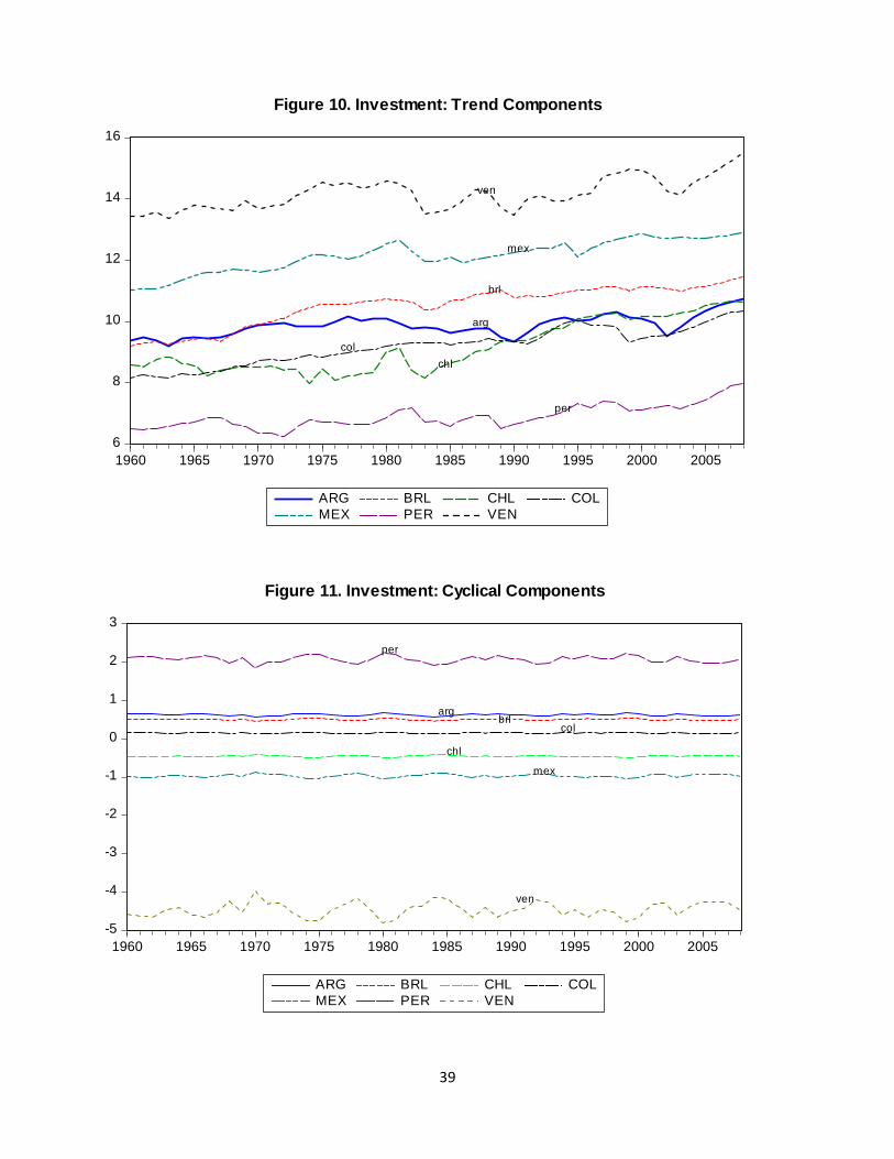
Investment: the trend-cycle decomposition of investment is plotted in figure 10 and 11

respectively. Our empirical evidence indicates that there is at least one cointegrating vector in

investment series of seven Latin American economies. This result suggests that there is not a

single source of common long run movements to generate a synchronized movement in these

economies. More importantly, investment in these economies is driven by more than one

common trends. Figure 10 displays the permanent components of investment in seven Latin

American economies. The volatility in trend components is distinct and apparent. The long-run

dynamics are captured by the upward and downward movement of trend components. This

indicates that permanent shocks have played a key role in determining investment decisions.

This is also justified by the stylized fact that investment is the trend. It means that investment is

less likely to react cyclical. The long-run behavior of investment reflects the good and bad

times these countries have gone through over time. Latin America has a well established

history of crises and on top of that financial instability appears to have become the norm, rather

the exception (Edwards, 2003). From the trend figure we can see two notable instances among

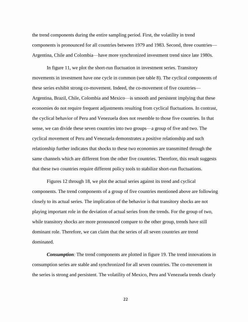
22

the trend components during the entire sampling period. First, the volatility in trend

components is pronounced for all countries between 1979 and 1983. Second, three countries—

Argentina, Chile and Colombia—have more synchronized investment trend since late 1980s.

In figure 11, we plot the short-run fluctuation in investment series. Transitory

movements in investment have one cycle in common (see table 8). The cyclical components of

these series exhibit strong co-movement. Indeed, the co-movement of five countries—

Argentina, Brazil, Chile, Colombia and Mexico—is smooth and persistent implying that these

economies do not require frequent adjustments resulting from cyclical fluctuations. In contrast,

the cyclical behavior of Peru and Venezuela does not resemble to those five countries. In that

sense, we can divide these seven countries into two groups—a group of five and two. The

cyclical movement of Peru and Venezuela demonstrates a positive relationship and such

relationship further indicates that shocks to these two economies are transmitted through the

same channels which are different from the other five countries. Therefore, this result suggests

that these two countries require different policy tools to stabilize short-run fluctuations.

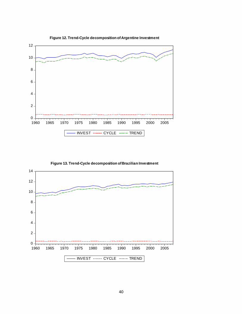
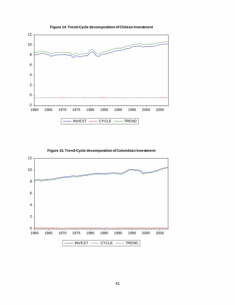
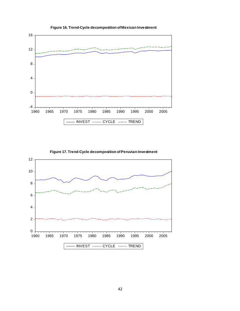
Figures 12 through 18, we plot the actual series against its trend and cyclical

components. The trend components of a group of five countries mentioned above are following

closely to its actual series. The implication of the behavior is that transitory shocks are not

playing important role in the deviation of actual series from the trends. For the group of two,

while transitory shocks are more pronounced compare to the other group, trends have still

dominant role. Therefore, we can claim that the series of all seven countries are trend

dominated.

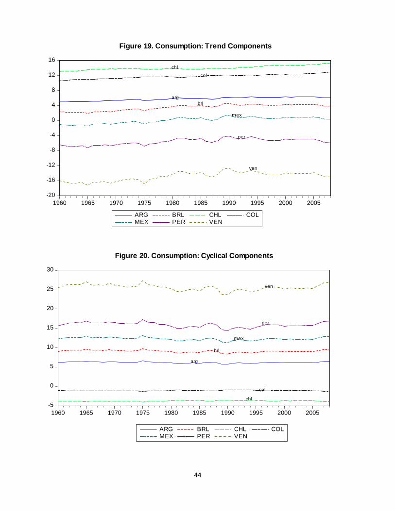
Consumption: The trend components are plotted in figure 19. The trend innovations in

consumption series are stable and synchronized for all seven countries. The co-movement in

the series is strong and persistent. The volatility of Mexico, Peru and Venezuela trends clearly

23

stand out from other countries. The trend components of Mexico, Venezuela and Peru are

below zero suggesting that consumption is not trended, it is a cyclical phenomenon. In other

words, private consumption of these countries follow the short-run cycles—consume more at

the time of economic boom and vice versa. The trend for these three economies peak around

1989-1990 followed by down turn in their consumption. Nonetheless, the co-movement is

strong the entire sampling period. Similarly, we can also observe a strong co-movement in

cyclical components of consumption. Figure 20 displays the effect of transitory innovations to

consumption. One striking characteristic of the cyclical components of consumption is that

economic prosperity (during period of 1984-1990) is accompanied by higher level of

consumption. This behavior is consistent with economic theory that asserts that consumption

depends on income.

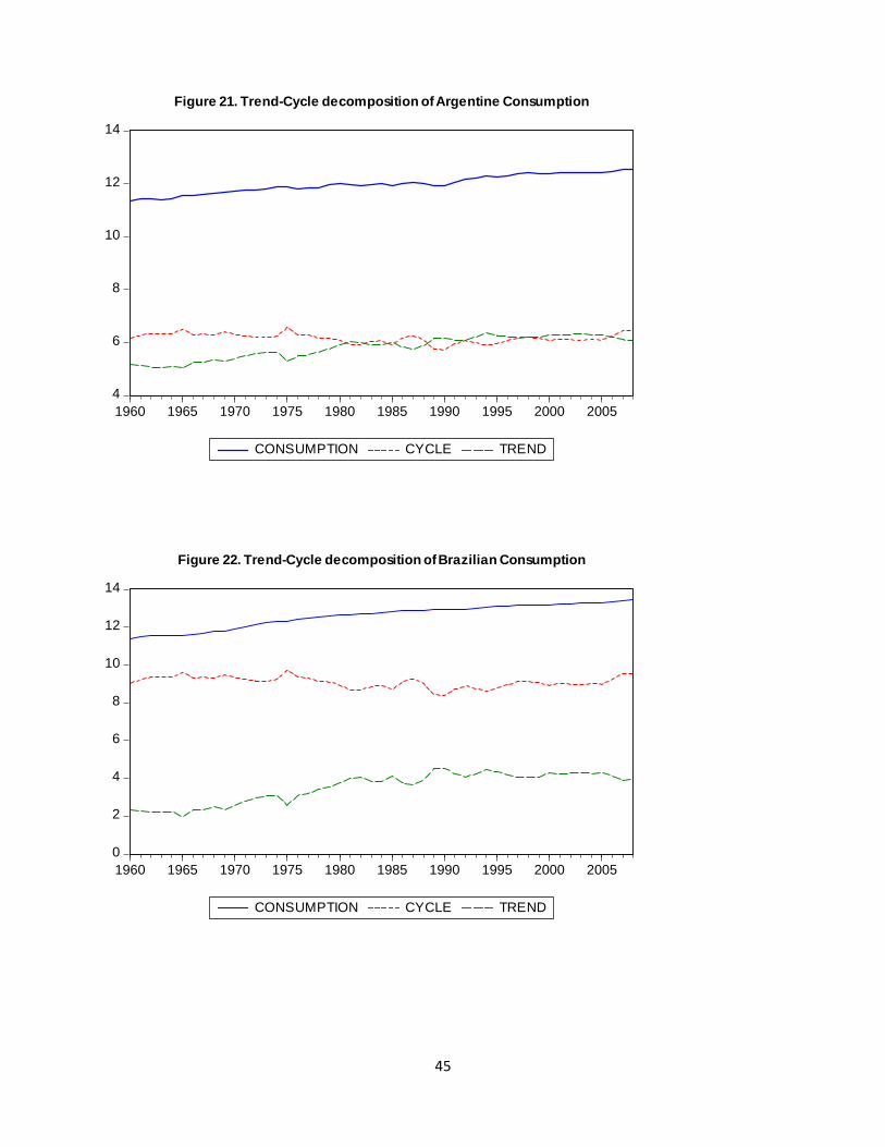
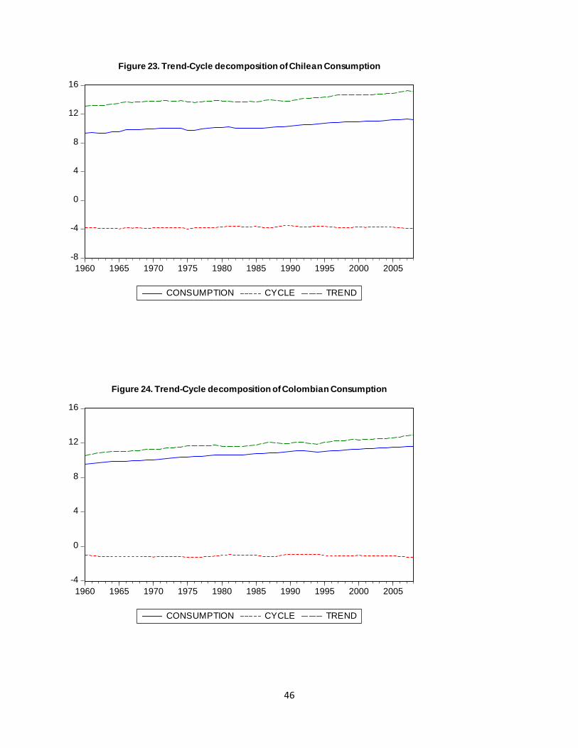
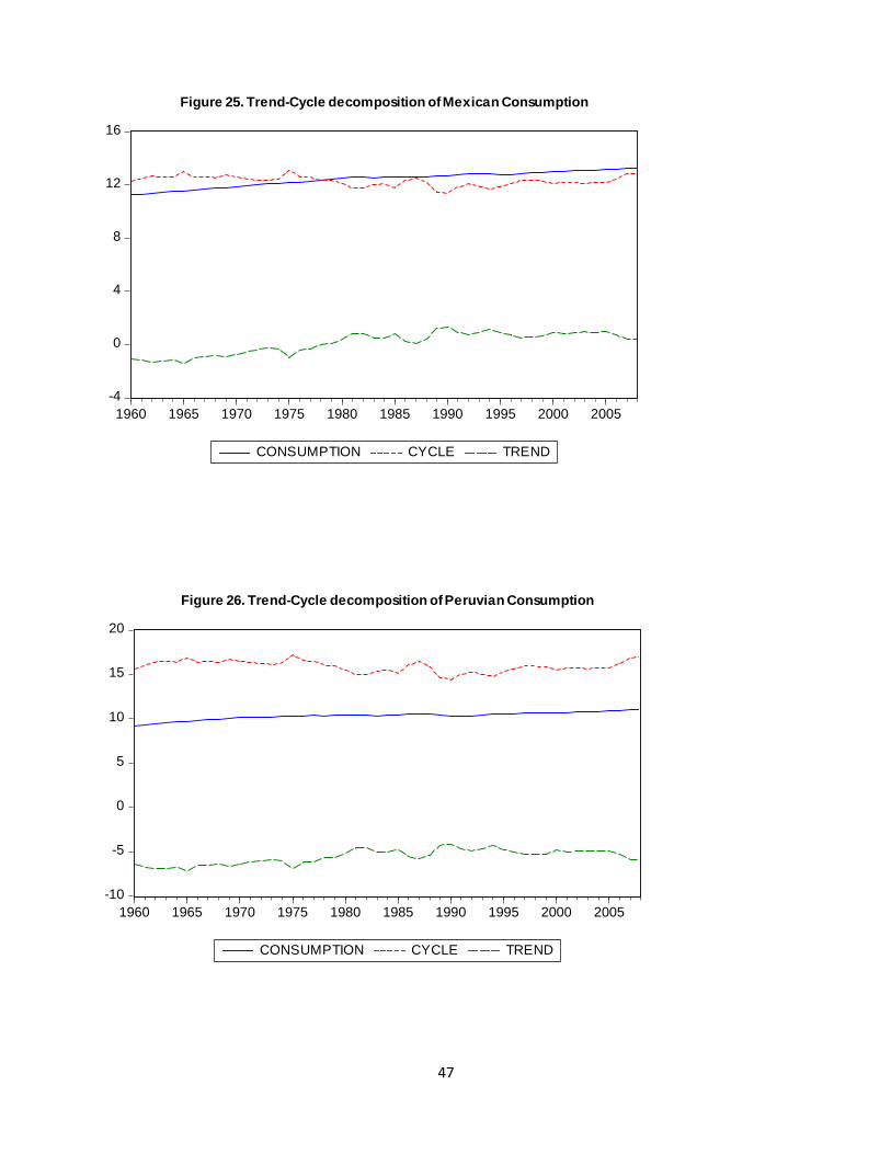
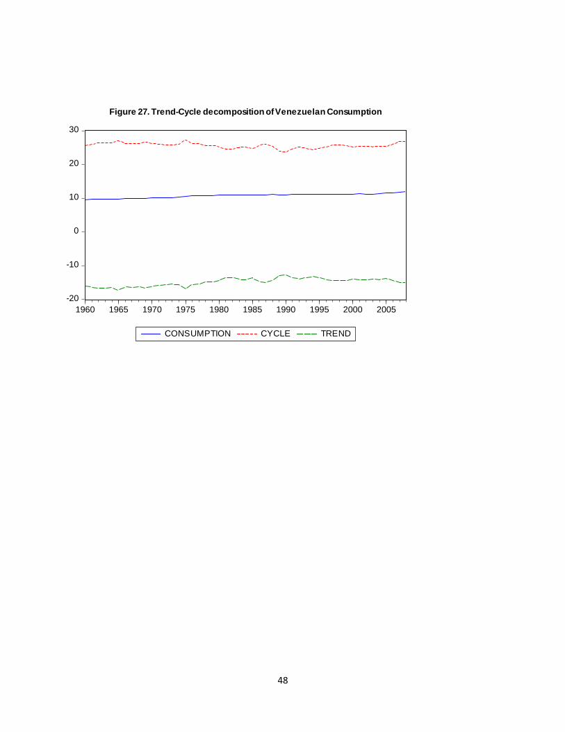
We plot the actual series of consumption against its trend and cyclical component in

figures 21 through 27. Out of seven countries, the transitory shocks seem to play a vital role in

determining consumption in the short-run for Brazil, Mexico, Peru and Venezuela since the

cyclical components are closely following or are above the actual consumption. So the

consumption of these four countries is cycle dominated. However, the cyclical components are

not a decisive factor for Chile and Colombia. The actual-trend relationship assures that the

consumption pattern of these two countries is trend dominated. The graphical evidence shows

that Argentine consumption is neither trend nor cycle dominated. Both the trends and cycles are

moving together staying away from the actual series. Together, five common trends and two

common cycles govern the stochastic behavior of the consumption behavior of these seven

countries.

24

5. Conclusion

By analyzing the long-term and short-term relationship among key macro variables—

real GDP, intra-regional trade, private investment and consumption—of seven largest Latin

American countries—Argentina, Brazil, Chile, Colombia, Mexico, Peru and Venezuela, we

find the existence of robust long-run economic relationship among these countries. The

Johansen cointegration results show that real output, trade, private investment and consumption

among these seven countries are driven by more one common trends. The existence of

cointegration implies that these countries share synchronous long-run movement in their macro

economies that give rise to greater economic integration in the region. The long-run

synchronous behavior of macro economy is necessary but not the sufficient condition in the

integration process (Abu-Aarn and Abu-Bader, 2008). The existence of short-run cycles

suffices the condition. Hence, we also compute the number of common cycles by using the

methodology proposed by Vahid and Engle (1993). The results produced from the multivariate

model indicate that these seven countries share common cycles in their macro variables. This

further reflects that these countries have shared the coordinated and common fiscal and

monetary policies over the study period.

The trend-cycle decomposition results display a number of interesting facts. We observe

that the transitory shocks to real GDP are not playing a major role, the major variation in the

actual series of real GDP is largely explained by the trend components. So the real GDP series

of all seven countries are trend-dominated. While empirical results indicate that these countries

share at least one common cycle in their investment series, the cyclical movement of Peru and

Venezuela is displaying an asynchronous behavior compared to the rest of the countries. In

light of this empirical evidence we conclude that these two countries require different policy

options to stabilize short-run disturbance in investment. The actual against trend-cycle plot

indicates that investments of all seven countries are trend dominated. In contrast, the

25

consumption pattern in these countries has produced some mixed results. The cyclical influence

is robust and decisive for consumption. Consumption for Brazil, Mexico, Peru, and Venezuela

seems to be cycle dominated whereas it is trend dominated for Chile and Colombia. Argentine

consumption is neither trend nor cycle dominated. The key finding from our trend-cycle

decomposition is that the economic fluctuation in these countries both in the long-run and

short-run follow a similar pattern in terms of their duration, intensity and timing.

Finally, the overwhelming evidences indicate among others mainly two policy

implications. First, since their macro economies are synchronized these countries can benefit

from harmonized monetary and fiscal policies. Second, the co-movement among macro

variables helps significantly in improving forecasting. Hence, we conclude that integration in

Latin American context is economically feasible.

26

References

Abu-Qarn, A. S.-B. (2008). On the optimality of a GCC Monetary Union: structural VAR,

common trends, and common cycles evidence. The World Economy , 31, 612-630.

Adom, A., Sharma, S. and Morshed, M (2010). Economic Integration in Africa. “Working

paper SIUC.”

Allegret, J. a.-Z. (2009). "Does a monetary union proect against external shock? An assessment

of Latin American integration". Journal of Policy Modeling , 31, p102-118.

Anderson, F.J. and Moazzami, B. (2003), ― Long-term trend and short-run dynamics of the

Canadian dollar: an error correction modeling approach‖, Applied Economics, 35, P1527-1530.

Anderson, H., & Kwark, N. a. (1999). "Does international trade synchronize business cycles? .

Monash University, Austrialia , Working paper 8/99.

Arnaudo, Aldo A. and Jacobo, Alejandro D. (1997), ―Macroeconomic homogeneity within

Mercosur: An overview‖, Estudios Economicos, 12, p 37-51.

Capannelli, G, Lee, j and Petri, P.A (2010),‖ Economic interdependence in Asia: developing

indicators for regional integration and cooperation‖ The Singapore Economic Review,55 p 125-

161.

Castillo, R. a. (2008). Economic Integration in North America. Applied Econometrics and

International Development , 8, p111-122.

Christodoulakis, N., & Dimelis, S. a. (1995). " Comparisions of business cycles in the EC:

Idiosyncrasies and Regularities". Economica , 62, p1-27.

Darrat, A. F.-S. (2005). On the path of integration in the Gulf region. Applied Economics , 37,

1055-1062.

Dickey, D.A., Jansen, D. W. and Thornton, D.L (1991), ― A primer on cointegration with an

application to money and income‖, Review, 73, No .2

Dickey, D.A. & Fuller, W.A, (1979), ― Distribution of the estimators for autoregressive time

series with a unit root‖, Journal of American Statistical Association, 74, No. 366, 427-431.

Dickey, D.A. & Fuller, W.A, (1981), ― Likelihood ratio statistics for autoregressive time series

with a unit root‖, Econometrica, 49(4), 1057-1072

Edwards, S. (2003), ―Financial instability in Latin America‖, Journal of International Money

and Finance, 22, 1095-1106.

27

Engle, R. a. (1993). " Common trends and common cycles in Latin America" . Revista

Brasileira de Economica , 47, p149-76.

Fiess, N. (2007). "Business cycle synchronization and regional integration: a case study for

Central America". The World Bank Economic Review , 21, p49-72.

Fiorito, R. a. (1994). "Stylized facts of Business Cycles in the G7 from a real business cycle

perspective" . European Economic Review , 38, p235-269.

Frankel, J.A. and Rose, A.K. (1998), ―The Endogeneity of the Optimum Currency Area

Criteria‖, Economic Journal, vol. 108, p1009-1025

Ffrench-Devis, R. ―Economic integration in Latin America‖,1989.

Fullerton, T. a. (1996). " New directions in Latin American macroeconometrics". Economic

and Business Review , 38, p49-73.

Haan, J. D and Montoya, L.A. (2008). "Regional business cycle synchronization in Europe?".

International Economics and Economic Policy , 5, p123-137.

Hernandez, J. (2004). "Business cycles in Mexico and the United States: do they share common

movements?". Journal of Applied Economies , VII, p303-323.

Jacobo, A. (2002). " Taking the business cycle's pulse to some Latin American Economies: is

there a rhythmical beat?". Estudios Economicos , 29, p219-245.

Johansen, S. (1988),‖Statistical analysis of cointegrating vectors‖ Journal of Economic

Dynamics and Control, 12(2-3) 231-254.

Kenen, P.B, and Meade, E.E .‖ Regional monetary integraton‖ Cambridge press 2008.

Krugman, Paul R. and Obsfeld, Maurice, ―International Economics, Addison Wesley, 2008.

Kwiatkowski, D., Phillips, P., Schmidt, P. and Shin, Y.(1992),‖Testing the null hypothesis of

stationary against the alternative of a unit root‖, Journal of Econometrics, 54(1-3), 159-178.

McAdam, P. (2007). USA, Japan and the Euro Area: Comparing business cycles features.

International Review of Applied Economics , 21, p135-156.

Mejia-Reyes, P. (1999), ―Classical business cycles in Latin America: turning points,

asymmetries and international synchronization‖, Estudios Economicos, 14,p2.

Mena, H. (1995). "Pushing the sisyphean Boulder? Macroeconometrics testing in Latin

American countries". Review of Income and Wealth , 10, p81-99.

Mundell, R. (1961). "A theory of optimum currency areas". The American Economic Review,

51, p657-665.

28

Phillips, P. and Perron, P (1988), ―Testing for a unit root in time series regression‖ Biometrika,

75(2) 335-346.

Rana, P. B. (2007). Economic integration and synchronization of business cycles in East Asia.

Journal of Asian Economics , 18, 711-25.

Rose, A. K. (2001). National money as a barrier to international trade: the real case for

currency union. American Economic Review , 91, 386-390.

Rosenthal, G. (1985). "The lessons of economic integration in Latin America; the case of

Central America". p139-158.

Sato, K. and zhang, Z (2006), ― Real output co-movements in East Asia: Any evidence for a

Monetary Union?‖, The World Economy, 29, 1671-1689.

Selover, D. (1999). " International transmission and business cycles transmission in ASEAN" .

Journal of the Japanese and the International Studies , 13, p230-253.

Sharma, S. a. (2002). " Long term trends and cycles in ASEAN stock markets". Review of

Financial Economics , 11, p299-315.

Sharma, S. C. (1997). Macroeconomic interdependence and integration in the Indian sub-

continent. Journal of quantitative economics , 13, 37-59.

Strydom, P. (1995). "International trade and economic growth: the opening up of the South

African Economy". The South African Journal of Economics, 63, p556-68.

Vahid, F. and Engle, R.F.(1993), ―Common trends and common cycles‖, Journal of Applied

Econometrics 8(4), 341-360.

Vasta, P. and Sharma, S.C. (2010), ―Monetary policy synchronization in the ASEAN-5 region:

an exchange rate perspective‖ working paper, SIUC

29

Table-1: Percentage of real GDP in the Latin American region

Year Argentina Brazil Chile Colombia Mexico Peru Venezuela

1980-1984 15.07 31.24 2.05 4.03 27.43 2.98 6.43

1985-1989 13.49 34.09 2.29 4.38 25.93 2.90 6.21

1990-1994 13.60 31.71 2.93 4.78 27.01 2.33 6.45

1995-1999 14.34 31.42 3.55 4.80 25.77 2.59 6.00

2000-2004 12.84 32.02 3.85 4.75 28.15 2.69 5.44

2005-2008 14.17 31.71 3.94 5.01 26.90 2.97 6.04

Source: World Development Indicators (2009).

Table 2: Intra-regional trade (% of the region)

Year Argentina Brazil Chile Colombia Mexico Peru Venezuela

1980-1984 22.29 13.76 21.34 19.19 6.24 13.95 27.52

1985-1989 26.36 12.49 19.96 18.40 5.44 18.63 18.19

1990-1994 33.68 19.28 20.67 24.39 5.76 26.72 29.28

1995-1999 38.49 23.29 24.22 26.56 4.10 25.13 27.65

2000-2004 41.04 20.79 27.22 29.73 4.13 25.82 32.00

2005-2008 41.69 22.68 23.31 32.73 5.84 28.18 29.09

Source: Direction of trade statistics year book.

30

Table 3: Unit Roots Test

Log levels

Variable Country ADF Test DF Test Phillips-Perron Test KPSS Test

tµ tτ tα* tα~ Z(Ф1) Z(Ф2) Z(Ф3) Z(τα*) Z(τα~)

RGDP

Argentina -0.230 -1.858 -0.38 -1.94 6.777 5.461 2.065 -0.375 -2.149 0.88

Brazil -3.062 -1.233 -3.46 -1.29 21.221 14.165 3.603 -2.628 -1.421 0.86

Chile 0.332 -1.750 0.36 -1.41 13.877 10.058 1.479 0.238 -1.697 0.90

Colombia -1.580 -1.721 -3.07 -1.50 62.045 42.122 3.720 -2.441 -1.616 0.91

Mexico -3.572 -1.731 -4.12 -1.85 48.330 33.018 8.184 -3.922 -1.887 0.89

Peru -0.427 -2.279 -0.96 -1.96 8.285 6.962 2.415 -0.995 -2.251 0.88

Venezuela -1.130 -2.947 -1.34 -2.50 7.812 7.232 3.486 -1.351 -2.668 0.90

TRADE

Argentina 0.127 -2.534 -0.16 -1.55 3.080 3.308 1.763 -0.356 -1.982 0.69

Brazil 0.338 -1.398 -0.06 -1.67 3.761 3.858 2.067 -0.22 -2.15 0.71

Chile 1.126 -3.183 0.65 -1.64 5.088 5.576 2.140 0.43 -1.87 0.70

Colombia 0.573 -3.987 0.08 -2.00 6.570 5.563 2.374 0.10 -2.31 0.72

Mexico -0.116 -5.023 -0.67 -2.17 5.004 5.18 3.07 -0.74 -2.65 0.72

Peru 0.006 -3.238 -0.57 -2.49 4.25 4.75 3.61 -0.55 -2.89 0.72

Venezuela -0.039 -1.349 -6.89 -7.06 0.97 1.75 1.58 -0.39 -1.70 0.58

INVEST

Argentina -1.523 -2.622 -1.08 -1.92 1.33 2.00 2.39 -1.26 -2.25 0.56

Brazil -1.379 -2.025 -1.55 -1.76 5.48 3.97 2.05 -1.57 -1.91 0.83

Chile -0.215 -2.253 -0.39 -2.37 1.04 2.66 2.85 -0.04 -2.26 0.79

Colombia -0.389 -2.849 -0.57 -2.16 3.24 4.05 3.14 -0.67 -2.62 0.83

Mexico -1.698 -2.651 -1.84 -2.64 5.17 4.54 3.68 -1.92 -2.67 0.84

Peru -0.275 -3.411 -0.87 -2.36 0.81 2.43 3.06 -0.81 -2.45 0.77

Venezuela -1.524 -2.585 -1.66 -2.69 1.48 2.66 3.31 -1.42 -2.73 0.64

CONS.

Argentina -0.911 -3.43 -1.00 -2.77 5.83 5.72 3.83 -1.00 -2.89 0.90

Brazil -2.426 -1.024 -2.79 -1.03 27.19 17.83 2.99 -2.41 -1.19 0.88

Chile -0.475 -2.042 -0.67 -2.21 5.68 4.79 2.54 -0.65 -2.38 0.88

Colombia -0.927 3.011 -1.74 -2.17 33.28 22.88 3.52 -1.73 -2.33 0.92

Mexico -2.353 -2.125 -3.48 -1.77 45.15 31.01 6.29 -3.37 -1.82 0.90

Peru -1.592 -2.853 -3.82 -4.06 14.31 13.62 8.94 -3.18 -3.73 0.84

Venezuela -0.600 -1.877 -1.04 -1.36 9.45 7.00 1.48 -0.98 -1.71 0.87

31

Table 4: Unit Roots Test

Log first difference

Variable Country ADF Test DF Test Phillips-Perron Test KPSS

Test tµ tτ tα* tα~ Z(Ф1) Z(Ф2) Z(Ф3) Z(τα*) Z(τα~)

RGDP

Argentina -5.716 -5.670 -5.78 -5.72 16.14 9.74 14.61 -5.85 -5.86 0.10

Brazil -4.033 -4.227 -3.93 -4.17 9.48 6.16 9.21 -4.15 -4.46 0.40

Chile -4.966 -4.992 -5.06 -5.04 8970.20 8.02 12.02 -5.11 -5.14 0.17

Colombia -4.415 -4.651 -4.23 -4.69 9.32 7.40 11.07 -4.44 -4.92 0.28

Mexico -4.564 -5.326 -4.38 -5.27 9.54 8.97 13.44 -4.50 -5.42 0.53

Peru -4.261 -4.191 -4.29 -4.22 8.28 6.96 2.41 -4.21 -4.16 0.23

Venezuela -5.596 -5.552 -5.61 -5.58 15.42 10.10 15.15 -5.71 -5.74 0.16

TRADE

Argentina -4.240 -4.399 -4.51 -4.58 12.42 7.44 11.12 -4.75 -4.87 0.10

Brazil -4.829 -5.043 -5.20 -5.29 16.88 9.67 14.48 -5.39 -5.56 0.11

Chile -3.655 -4.202 -3.81 -4.17 15.14 6.06 9.07 -4.06 -4.43 0.22

Colombia -5.035 -5.239 -5.41 -5.46 14.66 10.06 15.07 -5.60 5.77 0.14

Mexico -4.173 -4.286 -4.05 -3.97 1796.14 4.85 7.23 -4.12 -4.12 0.07

Peru -6.108 -6.516 -6.88 -7.05 46.61 18.97 28.17 -6.94 -7.59 0.10

Venezuela -4.837 -5.062 -4.90 -5.06 12.00 8.73 13.08 -5.07 -5.46 0.18

INVEST

Argentina -5.425 -5.425 -5.50 -5.49 15.56 9.52 14.28 -5.53 -5.59 0.09

Brazil -5.816 -5.788 -5.81 -5.80 16.69 10.89 16.35 -5.91 -5.96 0.12

Chile -7.268 -7.331 -7.44 -7.47 97.09 20.96 31.45 -7.89 -8.23 0.30

Colombia -5.529 -5.484 -5.71 -5.65 16.26 10.57 15.86 -5.85 -5.86 0.05

Mexico -6.478 -6.481 -6.43 -6.46 53.49 13.91 20.86 -6.59 6.73 0.15

Peru -5.800 -5.888 -5.45 -5.48 14.09 9.28 13.91 -5.45 -5.56 0.29

Venezuela -7.055 -6.993 -7.14 -7.07 32.84 18.38 27.58 -7.71 -7.73 0.19

CONS.

Argentina -5.785 -5.722 -5.82 -5.76 16.37 10.54 15.77 -5.89 -5.90 0.31

Brazil -5.290 -5.541 -5.21 -5.56 14.96 10.82 16.22 -5.54 -5.89 0.38

Chile -7.164 -7.095 -7.24 -7.16 27.71 17.21 25.79 -7.42 -7.42 0.06

Colombia -4.936 -4.951 -4.73 -4.82 12.49 6.85 10.21 -4.64 -4.78 0.12

Mexico -4.390 -4.894 -4.20 -4.86 9.38 7.25 10.87 -4.24 -4.90 0.49

Peru -3.992 -3.912 -4.00 -3.92 7.92 4.76 7.12 -3.92 3.88 0.35

Venezuela -4.122 -4.068 -4.14 -4.11 8.36 5.41 8.11 -4.23 -4.23 0.14

32

Table 5: Johansen’s Cointegration tests

Variables Eigenvalues H0 λ-trace λ-max 95% quantiles CV

λ-trace λ-max

RGDP

0.686 r ≤ 0 160.46* 54.43* 125.61 46.23

0.651 r ≤ 1 106.03* 49.50* 95.75 40.07

0.454 r ≤ 2 56.53 28.46 69.82 33.87

0.224 r ≤ 3 28.06 11.94 47.85 27.58

0.170 r ≤ 4 16.12 8.81 29.79 21.13

0.122 r ≤ 5 7.30 6.12 15.49 14.26

0.025 r ≤ 6 1.19 1.19 3.84 3.84

TRADE

0.889 r ≤ 0 186.48* 63.95* 125.61 46.23

0.792 r ≤ 1 122.53* 45.50* 95.75 40.07

0.734 r ≤ 2 77.03* 38.38* 69.82 33.87

0.542 r ≤ 3 38.65 22.65 47.85 27.58

0.284 r ≤ 4 16.01 9.69 29.79 21.13

0.184 r ≤ 5 6.31 5.89 15.49 14.26

0.014 r ≤ 6 0.42 0.42 3.84 3.84

INVEST

0.705 r ≤ 0 147.32* 56.13* 125.61 46.23

0.495 r ≤ 1 91.18 31.41 95.75 40.07

0.429 r ≤ 2 59.78 25.82 69.82 33.87

0.325 r ≤ 3 33.95 18.12 47.85 27.58

0.196 r ≤ 4 15.84 10.03 29.79 21.13

0.117 r ≤ 5 5.81 5.75 15.49 14.26

0.001 r ≤ 6 0.06 0.06 3.84 3.84

CONS.

0.682 r ≤ 0 159.67* 52.78* 125.61 46.23

0.592 r ≤ 1 106.89* 41.31* 95.75 40.07

0.463 r ≤ 2 65.57 28.65 69.82 33.87

0.346 r ≤ 3 36.92 19.55 47.85 27.58

0.194 r ≤ 4 17.36 9.95 29.79 21.13

0.141 r ≤ 5 7.41 7.02 15.49 14.26

0.008 r ≤ 6 0.38 0.38 3.84 3.84

* indicates rejection of the null hypothesis at 5% significance level.

33

Table 6: Lagrange Multiplier test for serial correlation

Variables Lags χ2

(49) P- value

RGDP 1 58.39 0.16

TRADE 1 66.58 0.05

INVEST 2 48.56 0.49

CONS. 2 40.25 0.81

* the null hypothesis is that there is no serial correlation

Table 7: Likelihood Ratio test for Individual significance

Variable Country χ2

(2) p-value

RGDP

Argentina 23.18 0.00

Brazil 18.52 0.00

Chile 20.36 0.00

Colombia 13.06 0.00

Mexico 11.57 0.00

Peru 4.66 0.09

Venezuela 20.40 0.00

TRADE

Argentina

26.17

0.00

Brazil 28.22 0.00

Chile 29.02 0.00

Colombia 16.58 0.00

Mexico 25.03 0.00

Peru 36.30 0.00

Venezuela 13.22 0.00

INVEST.

Argentina

χ2

(1)

15.63

0.00

Brazil 1.81 0.17

Chile 17.52 0.00

Colombia 8.73 0.00

Mexico 13.65 0.00

Peru 23.13 0.00

Venezuela 8.38 0.00

CONS.

Argentina 17.31 0.00

Brazil 12.63 0.00

Chile 8.12 0.01

Colombia 5.88 0.05

Mexico 6.73 0.03

Peru 22.60 0.00

Venezuela 9.46 0.00

34

Table 8: Test for the number of common cycles

Null ρi2 C(p*,s) df F-stat

Real GDP

s = 1

0.03

1.43

3

0.59

s = 2 0.10 6.36 8 0.91

s = 3 0.16 14.55 15 1.02

s = 4 0.23 26.83 24 1.13

s = 5 0.29 42.93 35 1.20

s = 6 0.40 66.94 48 1.36*

s = 7 0.74 130.25 63 2.17*

TRADE

s =1

0.02 0.59 4 0.23

s = 1 0.04 1.77 10 0.22

s = 2 0.21 8.61 18 0.50

s = 3 0.30 18.95 28 0.64

s = 4 0.62 47.01 40 1.13

s = 5 0.73 84.98 54 1.57*

s = 6 0.92 158.23 70 2.60*

INVEST

s =0

0.06 2.91 9 0.25

s =1 0.11 8.39 20 0.28

s =2 0.15 16.02 33 0.31

s =3 0.25 29.54 48 0.40

s = 4 0.36 50.52 65 0.51

s =5 0.67 102.63 85 0.84

s =6 0.80 178.27 105 1.27*

CONS.

s =1

0.00 0.00 2 0.09

s =2 0.01 0.47 8 0.11

s =3 0.05 2.88 15 0.22

s =4 0.27 17.67 24 0.74

s =5 0.38 40.14 35 1.12

s =6 0.51 73.67 48 1.51*

s= 7 0.71 131.85 63 2.19*

*indicates rejection of the null hypothesis at 10% significance level.

34

7

8

9

10

11

12

13

14

1960 1965 1970 1975 1980 1985 1990 1995 2000 2005

ARG BRL CHL COL

MEX PER VEN

Figure 1. Real GDP: Trend components

col

per

mex

chi

brl

ven

arg

-1.0

-0.5

0.0

0.5

1.0

1.5

2.0

2.5

3.0

1960 1965 1970 1975 1980 1985 1990 1995 2000 2005

ARG BRL CHL COL

MEX PER VEN

Figure 2. Real GDP: cyclical components

arg

brl

chl

col

mex

per

ven

35

0

2

4

6

8

10

12

14

1960 1965 1970 1975 1980 1985 1990 1995 2000 2005

RGDP CYCLE TREND

Figure 3. Trend-cycle decomposition of Argentina's Real GDP

0

2

4

6

8

10

12

14

1960 1965 1970 1975 1980 1985 1990 1995 2000 2005

RGDP CYCLE TREND

Figure 4. Trend-Cycle decomposition of Brazilian Real GDP

36

-2

0

2

4

6

8

10

12

14

1960 1965 1970 1975 1980 1985 1990 1995 2000 2005

RGDP CYCLE TREND

Figure 5. Trend-Cycle decomposition of Chilian Real GDP

0

2

4

6

8

10

12

1960 1965 1970 1975 1980 1985 1990 1995 2000 2005

RGDP CYCLE TREND

Figure 6.Trend-Cycle decomposition of Colombian Real GDP

37

0

2

4

6

8

10

12

14

1960 1965 1970 1975 1980 1985 1990 1995 2000 2005

RGDP CYCLE TREND

Figure 7. Trend-Cycle decomposition of Mexican Real GDP

0

2

4

6

8

10

12

1960 1965 1970 1975 1980 1985 1990 1995 2000 2005

RGDP CYCLE TREND

Figure 8. Trend-Cycle decomposition of Peruvian Real GDP

38

0

2

4

6

8

10

12

14

1960 1965 1970 1975 1980 1985 1990 1995 2000 2005

RGDP CYCLE TREND

Figure 9. Trend-Cycle decomposition of Venezuelan Real GDP

39

6

8

10

12

14

16

1960 1965 1970 1975 1980 1985 1990 1995 2000 2005

ARG BRL CHL COL

MEX PER VEN

Figure 10. Investment: Trend Components

arg

brl

chl

col

mex

per

ven

-5

-4

-3

-2

-1

0

1

2

3

1960 1965 1970 1975 1980 1985 1990 1995 2000 2005

ARG BRL CHL COL

MEX PER VEN

Figure 11. Investment: Cyclical Components

argbrl

chl

col

mex

per

ven

40

0

2

4

6

8

10

12

1960 1965 1970 1975 1980 1985 1990 1995 2000 2005

INVEST CYCLE TREND

Figure 12. Trend-Cycle decomposition of Argentine Investment

0

2

4

6

8

10

12

14

1960 1965 1970 1975 1980 1985 1990 1995 2000 2005

INVEST CYCLE TREND

Figure 13. Trend-Cycle decomposition of Brazilian Investment

41

-2

0

2

4

6

8

10

12

1960 1965 1970 1975 1980 1985 1990 1995 2000 2005

INVEST CYCLE TREND

Figure 14. Trend-Cycle decomposition of Chilean Investment

0

2

4

6

8

10

12

1960 1965 1970 1975 1980 1985 1990 1995 2000 2005

INVEST CYCLE TREND

Figure 15. Trend-Cycle decomposition of Colombian Investment

42

-4

0

4

8

12

16

1960 1965 1970 1975 1980 1985 1990 1995 2000 2005

INVEST CYCLE TREND

Figure 16. Trend-Cycle decomposition of Mexican Investment

0

2

4

6

8

10

12

1960 1965 1970 1975 1980 1985 1990 1995 2000 2005

INVEST CYCLE TREND

Figure 17. Trend-Cycle decomposition of Peruvian Investment

43

-8

-4

0

4

8

12

16

1960 1965 1970 1975 1980 1985 1990 1995 2000 2005

INVEST CYCLE TREND

Figure 18. Trend-Cycle decomposition of Venezuelan Investment

44

-20

-16

-12

-8

-4

0

4

8

12

16

1960 1965 1970 1975 1980 1985 1990 1995 2000 2005

ARG BRL CHL COL

MEX PER VEN

Figure 19. Consumption: Trend Components

arg

brl

chl

col

mex

per

ven

-5

0

5

10

15

20

25

30

1960 1965 1970 1975 1980 1985 1990 1995 2000 2005

ARG BRL CHL COL

MEX PER VEN

Figure 20. Consumption: Cyclical Components

arg

brl

chl

col

mex

per

ven

45

4

6

8

10

12

14

1960 1965 1970 1975 1980 1985 1990 1995 2000 2005

CONSUMPTION CYCLE TREND

Figure 21. Trend-Cycle decomposition of Argentine Consumption

0

2

4

6

8

10

12

14

1960 1965 1970 1975 1980 1985 1990 1995 2000 2005

CONSUMPTION CYCLE TREND

Figure 22. Trend-Cycle decomposition of Brazilian Consumption

46

-8

-4

0

4

8

12

16

1960 1965 1970 1975 1980 1985 1990 1995 2000 2005

CONSUMPTION CYCLE TREND

Figure 23. Trend-Cycle decomposition of Chilean Consumption

-4

0

4

8

12

16

1960 1965 1970 1975 1980 1985 1990 1995 2000 2005

CONSUMPTION CYCLE TREND

Figure 24. Trend-Cycle decomposition of Colombian Consumption

47

-4

0

4

8

12

16

1960 1965 1970 1975 1980 1985 1990 1995 2000 2005

CONSUMPTION CYCLE TREND

Figure 25. Trend-Cycle decomposition of Mexican Consumption

-10

-5

0

5

10

15

20

1960 1965 1970 1975 1980 1985 1990 1995 2000 2005

CONSUMPTION CYCLE TREND

Figure 26. Trend-Cycle decomposition of Peruvian Consumption

48

-20

-10

0

10

20

30

1960 1965 1970 1975 1980 1985 1990 1995 2000 2005

CONSUMPTION CYCLE TREND

Figure 27. Trend-Cycle decomposition of Venezuelan Consumption