China’s Economic Growth 1978-2025: What We Know Today about China’s Economic Growth Tomorrow

Views of the future China vary widely. While some believe that the collapse of China is inevitable, others see the emergence of a new superpower that increasingly poses a threat to the U.S. This paper examines the economic growth prospects of China over the next two decades. Extrapolating past real GDP growth rates into the future, the size of the Chinese economy surpasses that of the U.S. in purchasing power terms between 2012 and 2015; by 2025, China is likely to be the world's largest economic power by almost any measure. The extrapolations are supported by two types of considerations. First, China’s growth patterns of the past 25 years since the beginning of economic reforms match well those identified by standard economic development and trade theories (structural change, catching up, and factor price equalization). Second, decomposing China’s GDP growth into growth of labor and other variables, the near-certain information available today about the quantity and quality of Chinese laborers through 2015, if not several years after, allows inferences about future GDP growth. Short of some cataclysmic event, demographics alone suggests China’s continued economic rise. If talent is randomly distributed in the world population and if agglomeration of talent is important, then the odds are strongly in China’s favor. JEL codes: O1 (O10, O11), O4 (O40, O47), O53, J11, O3, I21 Keywords: economic growth, growth accounting, growth forecasts, development theories, human capital

formation, education (all: China)

Carsten A. Holz Social Science Division, Hong Kong University of Science & Technology

Clear Water Bay, Kowloon, Hong Kong E-mail: socholz@ust.hk; Tel/Fax: +852 2719-8557

I am grateful for comments from seminar/ panel participants at the Center for East Asian Studies, Stanford University (23 February 2004), the Association for Asian Studies meetings, San Diego (5 March 2004), the Universities Service Center for China Studies, Hong Kong (30 June 2005), the Western Economic Association Meetings 2005, San Francisco (7 July 2005), and the Center on China’s Transnational Relations, HKUST (30 September 2005). Thomas P. Lyons has provided suggestions at various turns, and the paper has benefited from communication with Thomas G. Rawski on Chinese statistics. A grant from the Research Grants Council of Hong Kong (Project no. HKUST 6122/03H) provided financial support.

2 November 2005 (minor stylistic revision of 3 July 2005 version)

1. Introduction The rapid economic growth of China since the beginning of the economic reforms in 1978 has captured the imagination of Western commentators and researchers. The responses range from outright pessimism about China’s future to fear of a strong China. Lester Brown (1995) wonders who will feed China. Gordon Chang (2000) announces the coming collapse of China. Callum Henderson (1999) sees China as on the “brink,” while Ross Terrill (2003) writes of the “illusory nature of the market in most of the Chinese economy” and that “a crash looms because the Leninist core of the regime is unchanged from Mao’s construction of it in Yan’an six decades ago” (pp. 329, 313). Nicholas Lardy (1998) stresses the large economic problems and the unprecedented potential for social unrest due to ever more indebted state-owned enterprises, the extent of nonperforming loans, and a decline in government revenue. At the other end of the range are those who project a strong China. Geoffrey Murray (1998) describes China as the next superpower. A number of authors view an all-powerful China as a threat (Bill Gertz, 2000, or Edward Timperlake and William Triplett II, 2002).1 News items imploring the “devastation Chinese competitors are inflicting on U.S. industries, from kitchenware and car tires to electronic circuit boards” and the “futility of trying to match the China price” have become common fare.2

What is undeniable is China’s rapid economic growth over the past 25 years since the beginning of economic reforms in 1978, of, measured in gross domestic product (GDP), on average 9.37% per year. In economic size China is surpassed today only by the U.S., Japan, Germany, and France.3 Its share in global growth 1995-2002 has been estimated at 25%, compared to 20% for the U.S.4 While China’s economic growth has received much attention in the popular literature, China researchers, when it comes to economic growth, tend to focus on narrow topics, measuring total factor productivity growth in enterprises in different ownership forms or investigating the growth prospects of individual industries or firms. For example, Douglas Allen (2002) documents the transformation in four industries in China and predicts the imminent emergence of world-class Chinese brands. Ming Zeng and Peter Williamson (2003) examine the international growth prospects of Chinese firms (positive). Colin Carter and Scott Rozelle (2001) ask if China will become a major force in world food markets (yes, if structural transformation occurs). A number of studies try to explain China’s past economic growth. Much of the transition literature explains past reform successes—usually, if only implicitly, measured as economic growth—through institutional changes (for example, Qian Yingyi, 2000, 2003, or Wing Thye Woo, 1994, 1999). Justin Lin, Cai Fang, and Li Zhou (2003) explain China’s reform success with adoption of a “comparative-advantage following strategy,” allowing full play to China’s plentiful endowment with labor. Others analyze China’s past economic growth within the aggregate production function framework (Wang Yan and Yao Yudong, 2003; Wu Yanrui, 2004, Alwyn Young, 2000). The aggregate production function framework is also occasionally extended into the future. Gregory Chow and Kui-Wai Li (2002) estimate an economy-wide, aggregate production function for the years 1952-98 and obtain GDP values for the years through 2010 by extending variations of past factor input growth rates into the future; Gregory Chow

1

(2002) further includes an estimate of year 2020 GDP. A 1997 World Bank policy analysis of current economic issues is supplemented by an estimate of China’s GDP in 2020 based on a closed-economy model. A systematic study of future economic growth in China that makes full use of the hard facts already available today, however, is still lacking. Answers to the question of what we know today about the economic size of China ten or twenty years from now are relevant not only for the popular discourse on the new superpower and for China threat theorists and military strategists, but also for economists. For example, conventional economic wisdom holds that free trade benefits, by the laws of comparative advantage, all countries in the long run. Thus, a growing China, and growing trade between China and the U.S., benefits the U.S. But as Paul Samuelson (2004) within the framework of standard trade theory shows, a productivity gain in one country alone may, in fact, lead to a permanent loss in per capita real income in the other country; references to China abound. This paper examines China’s future economic growth in three steps. First, it conducts a straightforward extrapolation of a stable, past growth trend into the future. A number of scenarios are played through in a comparison with the U.S. But extrapolation is not a particularly convincing research tool. Why should the past continue into the future? One argument why past economic growth may continue into the future is that China’s economic growth matches standard growth patterns identified by theories of economic development and trade. These are structural change, catching up, and factor price equalization. China’s past economic growth fits well with all three. Furthermore, China’s reform period growth, within these three analytical frameworks, matches those of Japan, Korea, and Taiwan at an earlier stage of their development. Obviously, these four countries differ, as do the domestic and international circumstances under which they experienced a particular stage of development. But the differences need not be systematic with respect to the impact on the dependent variable economic growth. These growth patterns may well apply to China in the future, just as they already have to Japan, Korea, and Taiwan in the past. The final step is to decompose GDP growth. Growth accounting in the production function framework turns out to not be useful due to the lack of a stable aggregate production function over time. An alternative is to decompose GDP growth following the income approach to the calculation of GDP into growth of labor and of other variables. We already know today with near-certainty the size of China’s working age population through 2015, and can project with high reliability for several years after. In as far as gains in high school and university enrollment, most of them very recent, are unlikely to be reversed, a bottom line scenario on the quality of China’s future labor force can also be developed. Future GDP growth can be re-composed using solely the hard facts about the future quantity and quality of labor available today. Demographics in form of the quantity and quality of labor is enough to drive continued economic growth in China. Demographics means, for example, that for every “genius” in the U.S., China potentially has four. If talent is randomly distributed in the world population and if China’s education system is able to identify the brightest students, then China has a larger pool of talent to draw from than any other country in the world. If growth and innovation depend on the agglomeration of talent (geographically, nationally, culturally, or linguistically), then China

2

is in an excellent position to continue to grow and innovate. The recent explosion in tertiary level education may yet supply the productivity gains that Paul Samuelson identifies as potential causal factors for a permanent loss through trade in U.S. per capita real income. Projections cannot predict the future with certainty. Potential complications range from a collapse of Chinese Communist Party rule to war in the Taiwan Straits; China researchers ruminate about such issues as the bad loan problem in China’s banking system, loss-making state-owned enterprises, pilfered pension funds, local government budget deficits, rural-urban inequality, and environmental degradation. This paper works within these limitations. It does not attempt to provide an exhaustive list of complications, to examine the individual issues, to quantify their potential impact, and to attribute a likelihood to their occurrence. It predicts China’s future economic growth under the assumption that current and future problems continue to be resolved as they arise and that events of catastrophic dimensions do not occur.5 2. Extrapolation of Past Growth into the Future China’s year 2002 nominal GDP of 10.48 trillion RMB at the official exchange rate of approximately 8.277 RMB per USD translates into USD 1.27 trillion, compared to year 2002 U.S. GDP of 10.49 trillion.6 The U.S. economy in 2002, thus, was eight times larger than China’s economy; by 2004, following preliminary figures, the difference was seven-fold.7 However, such a comparison neglects to take into account the differing price levels in the two countries. The Penn World Tables (PWT), which report comparable GDP data in “international dollars,” assume that the general price level in China in 2000 was equivalent to only 23.13782% of the U.S. price level. The U.S. economy then, today, in purchasing power terms, is less than twice as large as China’s economy. Table 1 in the first row extrapolates PWT (version 6.1) data into the future. The PWT do not report economy-wide GDP. These values can, however, be obtained, by multiplying per capita GDP in international dollars (and constant 1996 prices, using the chain method) by the population numbers. Extrapolation into the future is based on year 2000 economy-wide GDP (in international dollars, at constant 1996 prices) because 2000 is the most recent year for which PWT data are available. The annual real GDP growth rate used to extrapolate into the future is the geometric mean of the period 1978-2000; 1978 is chosen as starting year since it marks the beginning of economic reforms in China. If China and the U.S. after 2000 each continue to grow with the same average annual growth rate they enjoyed between 1978 and 2000, then, as Table 1 reports, economy-wide GDP (in international dollars, at constant 1996 prices) of China surpasses that of the U.S. starting in 2015, a decade from now. But the manipulations of official Chinese data in the PWT may not be correct.8 The second scenario in Table 1 therefore uses the PWT year 2000 per capita GDP values (in international dollars, at constant 1996 prices) times population—accepting for the time being the PWT adjustments to Chinese data in levels—but then applies the average annual real GDP growth rate of the years 1978-2000 as implicit in the official data published by the Chinese National Bureau of Statistics (NBS) and the U.S. Bureau of Economic Analysis to the PWT GDP values.9 Using the official national data to obtain the average annual real GDP growth rate yields a larger

3

growth rate discrepancy in favor of China. Consequently, China’s aggregate purchasing power parity GDP begins to exceed that of the U.S. less than a decade from now, namely in 2012. The third scenario in Table 1 abandons both the PWT real growth rates and PWT GDP values. Instead, it uses national data (for details see notes to table). These are adjusted upward in the case of China by the PWT’s purchasing power parity factor of 4.321928 (1 divided by China’s price level of 23.13782% of the U.S. price level). The effect is almost the same as in the previous case. China’s aggregate purchasing power parity GDP now begins to exceed that of the U.S. in 2013 instead of 2012.10 The fourth scenario, using national base year data of the year 2002, the latest year for which final (revised) GDP values are available, and national average annual real growth rates of 1978-2002, yields a cross-over year of 2013. Assuming lower average annual real growth rates for China of 8% or even 7%, while maintaining that of the U.S. at 3%, the cross-over year moves further into the future to 2016 and 2020 (fifth and sixth row). The price adjustment factor in the case of China carries “substantial uncertainty” (Alan Heston, 2001, p. 1).11 The multiplicative factor of 4.321928 could be significantly off (in either direction). The seventh row in Table 1 reports the results if a smaller factor of 3 is used; in comparison to the PWT, this means underestimating China’s purchasing power parity GDP. In this case, the cross-over year is 2019. If the adjustment factor were to fall gradually over time—in the PWT it stayed virtually constant throughout the 1990s—assume from a value of 4 in 2002 to a value of 1 (no adjustment) in 30 years’ time, the cross-over year moves far into the future, namely to 2038 (eighth row). Since 2038 is more than 30 years into the future, this is the same as making no purchasing power adjustments at all (ninth row). Dropping the purchasing power concept and the PWT data altogether, but assuming a 3% appreciation in the official exchange rate every year after 2002 results in a cross-over year of 2026 (tenth row). In this scenario, the year 2002 exchange rate of 8.2770 yuan RMB/USD falls by approximately half to 4.0717 in 2026. Including, with the appreciation, some kind of price adjustment, which, even if only at a level of 2, currently makes eminent sense, would bring the cross-over year forward to 2019. The results reported so far covered aggregate nationwide GDP, with China overtaking the U.S. as early as 2012 in the scenario most (and not unrealistically) favorable to China and as late as 2038 in a highly unrealistic scenario. In terms of per capita GDP, the year when China surpasses the U.S. is far into the future (see additional columns in Table 1). But what is far into the future for the average Chinese person moves closer to the present for the richer areas of China. Little more than two decades from now, coastal China (as defined in the notes to Table 1), accounting for 41.54% of China’s population in 2000 and exceeding the U.S. population by 92.04%, may well be as rich, per capita, as the average U.S. citizen. Focusing on the five fastest-growing provinces in coastal China only, plus Shanghai, with a joint population in 2000 that is 27.14% larger than the U.S. population, moves the cross-over year in per capita GDP a few years further to the present. In other words, by the mid-2020s, a share of China’s population that exceeds the size of the U.S. population could enjoy the same standard of living as the U.S.; in addition, China has a per capita poorer hinterland with roughly three times the population in the richer areas.12

4

In these calculations, all variables were held constant except those explicitly allowed to vary. In particular, in the extrapolation of aggregate GDP, the use of an average annual past real growth rate reflects the product of the real GDP growth rate per capita and the population growth rate. In the short run, such as one decade, changes in the population growth rate are likely to be minor, but this may not hold in the long run. Similarly, the exchange rate was held constant except in the last two scenarios, as was the price adjustment factor except in the eighth through eleventh scenarios. The further into the future, the less valid are the assumptions. A more sophisticated approach would, furthermore, focus on the employed instead of the population.13 But none of these adjustments is likely to have a significant impact on the determination of cross-over years which are as little as one decade away. Extrapolations do not constitute a reliable research tool. Factors that promoted economic growth in the past may be absent in the future, or factors constraining economic growth may become newly relevant in the future. The next section examines explanations of economic growth. 3. Development Theories and Asian Precedents Explanations of China’s economic growth tend to focus on economic transition. The “success” of the reform process is explained by transition facts and strategies, where success is usually taken to imply economic growth (or a rise in living standards). For example, Wing-Thye Woo (1994) lists as crucial the creation of non-state firms in every sector of the economy, a high savings rate, good initial conditions (such as a small extent of central planning, unemployment in the countryside that could be taken up by township and village enterprises, or a limited social security net), historical conditions, and the Chinese Diaspora. Qian Yingyi (2000, 2003) ascribes much of China’s reform success to the unorthodox economic policy measures adopted by China’s leadership; the key to China’s economic growth was the unleashing of incentives and competition while making reform interest-compatible for those in power. Yet these explanations of past economic reform successes (and thus economic growth) face the problem of lack of a counterfactual. Wing-Thye Woo offers cross-country comparisons, but the number of explanatory variables appears larger than the number of comparison countries. Qian Yingyi makes an in part historical argument, but offers no explicit time series evaluation that examines the status before and after a particular reform measure was implemented. These explanations, thus, are not as strong as one might wish them to be.14 If one claims that economic transition “in total” has caused China’s past economic growth, then one could argue that key elements of transition have been in place since the early 1990s (price and domestic trade liberalization, the entry of private enterprises) and that therefore the gains from transition have already been exhausted. Consequently, economic growth should since have slowed, which it didn’t, or it could slow any time now. Alternatively, one could argue that past transition measures impact on economic growth over an extended period of time, or that transition is as yet incomplete, with further measures to go, in which cases the gains continue.

5

Growth patterns identified by economic theories of development and trade perhaps offer firmer ground. Economic transition could then be viewed as the removal of constraints that prevented well-known development patterns from unfolding.15 Furthermore, if China’s reform period growth patterns match those exhibited by other countries at stages in their economic development similar to China’s development level in the reform period, then China’s future growth patterns may also match those of the other economies later. The argument has two foundations: one is a focus on standard growth patterns, the other is a cross-country comparison with countries with which a comparison is likely to be meaningful. The growth patterns are structural change, catching up, and factor price equalization.16 These three patterns are not independent of each other, nor do they hold irrespective of the larger economic environment. They represent uni-causal explanations of economic growth that have the advantage that they do not rely on individual transition measures and have been identified by development economics and trade theory as of relevance. At the same time, in as far as they reveal China to be at the very early stages of accepted development patterns, they support the growth projections into the future. The comparison countries are Japan, Korea, and Taiwan. These three countries are relevant for China only if the assumption of constant effect among the four countries is met: different countries do not differ systematically with respect to the impact of the explanatory variable (specific to each growth pattern) on the dependent variable (economic growth). While these four countries differ, as do the domestic and international circumstances under which they experienced a particular stage of development, this does not necessarily invalidate the assumption of constant effect. The choice of countries to compare China to is a subjective choice, motivated only by the desire to make comparisons across a relatively homogeneous group of countries. China may share some economic growth patterns with Japan, Korea, and Taiwan due to cultural similarities, geographic location, similar economic development strategies, or, in the case of Japan, relatively large size of the domestic economy. Limiting the analysis to Japan, Korea, and Taiwan allows the careful compilation of the necessary data from each individual country’s statistical office, with a very few holes filled using the World Bank Development Indicators database, the International Financial Statistics (IFS), and the PWT.17 (The individual data sources are documented in Appendix 1.) An attempt was made to cover the years 1960 through 2002, with, in some instances, data available only beginning around 1970. Ideally, data for the 1950s should also have been included but are not available. The earlier in the development process of Japan, Korea, and Taiwan, the closer to the case of China the initial conditions might have been. Data on China are for the years of the reform period (the years since 1978). Throughout, the variable to be explained is real GDP growth per laborer since GDP is produced only by the active working population, namely laborers (one PWT figure, Figure 6, by necessity uses per capita figures). Employment data are midyear data when related to a variable that measures an annual flow, and end-year data otherwise (and then noted with the figure). Each data point in a figure is a particular country in a particular year.18

6

a. Structural change As labor shifts from low-productivity agriculture to higher-productivity industry and services, economy-wide real GDP per laborer, i.e., (partial) labor productivity, increases, if only because those laborers who have shifted sectors now produce a multiple of their former output value. Figure 1 shows just how big, and increasing, the labor productivity differences are between the three economic sectors in China. One would expect to see relatively high aggregate (economy-wide) labor productivity growth in those years when a relatively large number of laborers shifts out of agriculture. Figure 2 confirms the expectations. In years with a high absolute reduction in the share of laborers in agriculture, the growth rate of (real, likewise below) labor productivity is high. This pattern holds equally for all four countries. Among Japan, Korea, and Taiwan, the shift out of agriculture was, on average, fastest in Korea, followed by Taiwan and then Japan (Figure 3); this matches the initial shares of laborers in agriculture, with the highest one in Korea and the lowest one in Japan. One would consequently expect China, with an extremely high share of laborers in agriculture in 1978, to exhibit rapid reductions in this share, comparable perhaps to Korea, but the decline is more gradual. However, if in the official employment statistics the primary sector were obtained as residual, it could include an over time increasingly undercounted migrant population. The share of the primary sector in employment of, in 2002, approximately 50%, would then be an overestimate. At China’s 1978-2002 rate of decline, with an annual reduction in the share of laborers in agriculture by approximately an absolute value of 0.01 every year (thus, for example, from 0.7 to 0.69 in one year), China has another forty years to go before its agricultural labor share reaches the level of just below 10% at which Japan, Korea, and Taiwan appear to bottom out. Even if China’s primary sector employment of 2002 were somewhat overestimated, China still faces another two to three decades of labor transfers from the primary sector to the secondary and tertiary sector. But this implies that structural change as a source of economic growth has up to twenty to forty more years to contribute to labor productivity growth in China. Furthermore, in China, a given shift out of agriculture comes with higher labor productivity growth than in any of the other three countries. In Figure 2, the observations for China tend to lie above those of the other three countries. b. Catching up Catching up means that production techniques and technologies that have already been invented and implemented can be copied rather than need to be re-invented; technology transfer can also happen through the import of foreign equipment, possibly as part of foreign direct investment. Taking the U.S. as the leader in research and development, and proxying the level of technological development by labor productivity, the distance between a particular’s country labor productivity (in USD) and U.S. labor productivity serves as a measure of the potential scope for catching up. One would expect to see relatively high real GDP growth per laborer in those cases where the distance to the leading country (the U.S.) is relatively high, i.e., where the potential for catching up is large.19

7

Figure 4 confirms the hypothesis for Japan. Japan experienced its highest growth rates when its labor productivity was only ten to fifty percent of U.S. labor productivity. As the gap closed, growth rates in Japan fell (the trend curve shows a slight upswing at the highest labor productivity levels that appears to be an artifact of the imposed second-degree polynomial). Korea and Taiwan exhibit constantly high growth rates of labor productivity at around 4% to 6% throughout all years (Figure 4). But these two countries’ level of economic development is in the range of 5% to 50% of the U.S. level, which is a range in which Japan also exhibited high and constant labor productivity growth rates. Korea and Taiwan may yet have to experience the slow-down that comes when the potential gains from catching up are exhausted. China also exhibits a downward pattern, but at a much lower level of economic development. Figure 5 shows that China’s labor productivity between 1978 and 2002 was only 1.2 to 2.4 % of that of the U.S. (using the official exchange rate to translate Chinese yuan RMB values into USD values). This seems almost too narrow a band to determine long-term trends. As/if more observations become available at higher labor productivity levels relative to the U.S., the negative slope could well disappear or turn into a positive one. Whichever direction future observations are heading, at China’s highest level of catching up in the past, the growth rate of labor productivity was still at a relatively high 6-7%. Figure 6 replicates Figure 4 using PWT data. PWT data adjust for differing price levels across countries and may also, as in the case of China, undertake further adjustments to official data. Data are available for the 1950s through 1990s and are per capita (rather than per laborer); the observations for China are as always limited to the years since 1978. The pattern now is one of first rising labor productivity at low development levels before gradually falling off. This might reflect initial opening up effects as barriers to foreign direct investment and imports are removed and access to foreign knowledge increases. The Chinese observations are again concentrated in a very narrow band, with a negative slope. Independent of the choice of data, China is at a very low development level compared to the U.S. It appears to be at a stage of economic development (labor productivity) where other Asian countries started out more than 30 years ago. While labor productivity growth appears to fall as China catches up with the technology leader (and still is at a very high level), the scale of catching up is so small that such factors as exchange rate effects or uncertainties about the scale of the purchasing power adjustment could well render the slope coefficient insignificant. In the long run, as (if) China catches up with the U.S. and observations at higher development levels become available, the negative slope might yet turn into the positive slope that the other three countries exhibited at their earliest stage of economic development.20

c. Factor price equalization The factor price equalization theorem (or Heckscher-Ohlin-Samuelson theorem) states that factor prices, such as skill-specific wages, should equalize between two countries as long as a range of assumptions are met. I.e., the skill-specific wage rate of one country divided by that of the other country should equal unity.21 The slightly less restrictive, relative version of the factor price equalization theorem focuses on the relative prices of factors of production. Thus, for

8

example, a country with labor that is cheap relative to capital should see demand for its labor rise. As underemployed laborers become fully employed, labor productivity rises. An increase in the demand for labor may also be accompanied by wage rises, which in turn are likely to be accompanied by labor productivity growth.22 In the absence of reliable prices of capital, the price of capital is approximated here by the price of investment goods. The price of investment goods of any particular country relative to the U.S. is available in the PWT. Figure 7 reveals an inverse U-shaped pattern for all four countries. In other words, labor productivity growth first rises along with relative wage increases and then gradually falls as the relative return to factors of production in each country, vs. the U.S., approaches unity. In the case of China, also reproduced at a larger scale in Figure 8, the inverse U-shaped pattern occurs at an extremely low level, with wage rates in China, relative to investment prices, at only 2-5% of the corresponding U.S. ratio. This is well below the early levels of the other three Asian countries. Labor productivity growth in China is still high in the declining part of the inverse U-shaped pattern at 6-7%. Again, as more observations become available over time, the inverse U-shaped pattern may yet change. If this were just the beginning of a long-run trajectory, then the patterns of the other three Asian countries suggests that China’s potential for economic growth from relatively low labor costs will continue to exist for another thirty years.23 This section focused on three explanations of economic growth from development economics and trade theory and applied them to the case of China. China’s past economic growth matches these standard development patterns, as does economic growth in Japan, Korea, and Taiwan. In as far as China is located at the early stages of each pattern, in comparison to Japan, Korea, and Taiwan, there remains much scope for future gains in labor productivity and therefore growth. 4. Growth Accounting Growth accounting decomposes GDP growth into growth of variables other than GDP. I.e., growth of GDP is “explained” by the weighted growth rates of other variables. One need not view these other variables as constituting a satisfactory final explanation of GDP growth; for the purpose of forecasting future economic growth, regularity in the relationship with output suffices.24 If GDP growth and the growth of the variables into which it is decomposed exhibited a stable relationship in the past, and if this stable relationship is likely to continue into the future, then information about the future values of the variables into which GDP has been decomposed allows derivation of future GDP growth. One growth decomposition is the traditional decomposition of GDP growth into growth of different factor inputs. A second growth decomposition follows the income approach to the calculation of GDP. a. Decomposition of GDP growth into growth of factor inputs The traditional approach to growth accounting decomposes economic growth into growth of the factor inputs labor, capital, and “everything else” (also “technological progress,” or growth in total factor productivity, TFP). The traditional growth accounting equation is

9

(1) , tKtLt KbLbcY ˆˆˆ ++= where the hats denote growth rates, Y the value of constant-price output, L the (physical) quantity of laborers, and K the value of constant-price capital, or )ln()ln()ln()ln( tKtLOt KbLbtcAY +++= . Estimating the growth accounting equation for China for the period 1978 through 2002 (growth rates starting 1979), using annual data, yields , or ttt KLY ˆ2383.0ˆ2840.03609.6ˆ ++= (t-values) (1.1083) (0.4570) (0.4735) )ln(3975.0)ln(3859.00452.01769.4)ln( ttt KLtY +++= , (t-values) (1.4822) (1.0857) (1.4655) (1.0551) with the time variable t equal to one in 1978.25 Output is official year 2000 GDP with values for other years obtained by applying the latest published official real growth rates; the data on the midyear quantity of labor (including military personnel) and on the value of capital (in year 2000 prices) are explained in Carsten Holz (2005b, a). In both equations, all coefficients are insignificant.26 The residuals in both equations are normally distributed and homoskedastic, but according to the Durbin-Watson statistic or the Breusch-Godfrey serial correlation LM test positively serially correlated.27 Correcting for serial correlation also does not lead to significant coefficients. (For the data used here and below see Appendix 2.) China’s National Bureau of Statistics publishes nominal GDP values and real growth rates of GDP (but no explicit GDP deflator). Each year’s nominal GDP value is revised later, approximately one year after first published, but the real growth rates are usually, and implausibly, not revised. Using as measure of output in the growth accounting equation the official nominal GDP values deflated by the implicit deflator as first published (which is presumably final) yields no major changes in estimation results.28 Using as measure of output in the first equation a Tornqvist real growth rate of value-added aggregated across sectors, with official sectoral real growth rates weighted by sectoral nominal value-added shares (means of previous and current year), produces highly similar and also insignificant coefficients of labor and capital.29 The growth accounting equation can also be augmented by human capital. One approach is to include a direct measure of educational attainment in the growth accounting equation. For example, Wang Yan and Yao Yudong (2003) construct a human capital variable for the population in form of average years of schooling and enter it with the same weight in the growth accounting equation as labor. A second approach is to classify laborers by certain criteria, such as age and education, and to weight changes in the number of laborers in each category by their relative wages. Alwyn Young (2003), for example, adopts this second approach, and estimates relative wages from a mix of NBS household survey data of the years 1986-92 and Academy of Social Sciences household survey data of 1988 and 1995. This assumes that laborers were paid

10

their marginal product, at a time (prior to 1992/93) when most goods prices had not yet been liberalized and labor markets were virtually non-existent.30 Following the first approach and adding a human capital variable in the form of average years of education of laborers to the growth accounting equation yields , tttt HKLY ˆ5829.0ˆ4463.0ˆ2740.00390.5ˆ −++= (t-values) (0.8344) (0.4366) (0.7772) (-0.7771) where H denotes the average years of schooling across all laborers. Improvements in the average level of education appears to have a negative impact on GDP growth, but none of the coefficients is significant (and similarly if the growth accounting equation in logarithms is used), and the residuals are serially correlated (correcting for which does not lead to major differences in results).

The fact that all coefficients of the growth accounting equation (without or with human capital) are insignificant suggests that one or more assumption underlying the growth accounting equation is violated. The growth accounting equation can be derived following two different concepts (two different sets of assumptions). One is the concept of a production function, using, for example, the Cobb-Douglas production function, . The underlying assumptions are (i) the existence of an economy-wide aggregate production function (i.e., applicability of the Cobb-Douglas production function to economy-wide aggregates) and (ii) the particular functional form, which implies, among others, constant output elasticities (bL and bK do not depend on time).

KL bt

btt KLAY =

31 The second is the national income accounting concept. By the definition of GDP from the income side (more on which below), GDP can be written as Yt = wt Lt + rt Kt , where w denotes wages, and r the rental rate of capital (that parameter which makes the product with capital equal to GDP less labor remuneration). Assuming (i) constant factor shares and (ii) constant growth rates of wages and of the rental rate of capital, a few lines of manipulation yield the growth accounting equation.32 From the production function point of view, the immediate implication of insignificant coefficients is that output elasticities in China during the reform period were not constant over time. Further, estimation of an aggregate production function (growth accounting equation) works well in practice, even though the assumptions needed for aggregation are virtually never met, when aggregate data move little; aggregate data in China, over the reform period, however, changed manifold.33 From the point of view of the national income accounting identity, the growth rates of wages and of the rental rate of capital, with standard deviations of 0.0821 and 0.0443, are not sufficiently stable to yield the growth accounting equation as a tautology from the definition of GDP.34 Consequently, the coefficients in form of factor shares will not be accurately estimated. A simplification often imposed in the production function approach is to assume, for the Cobb-Douglas production function, constant returns to scale (bL=1-bK) and profit maximization in a competitive economy, so that output elasticities equal (constant) factor shares. The literature that incorporates human capital measures in growth accounting exercises for China indeed does

11

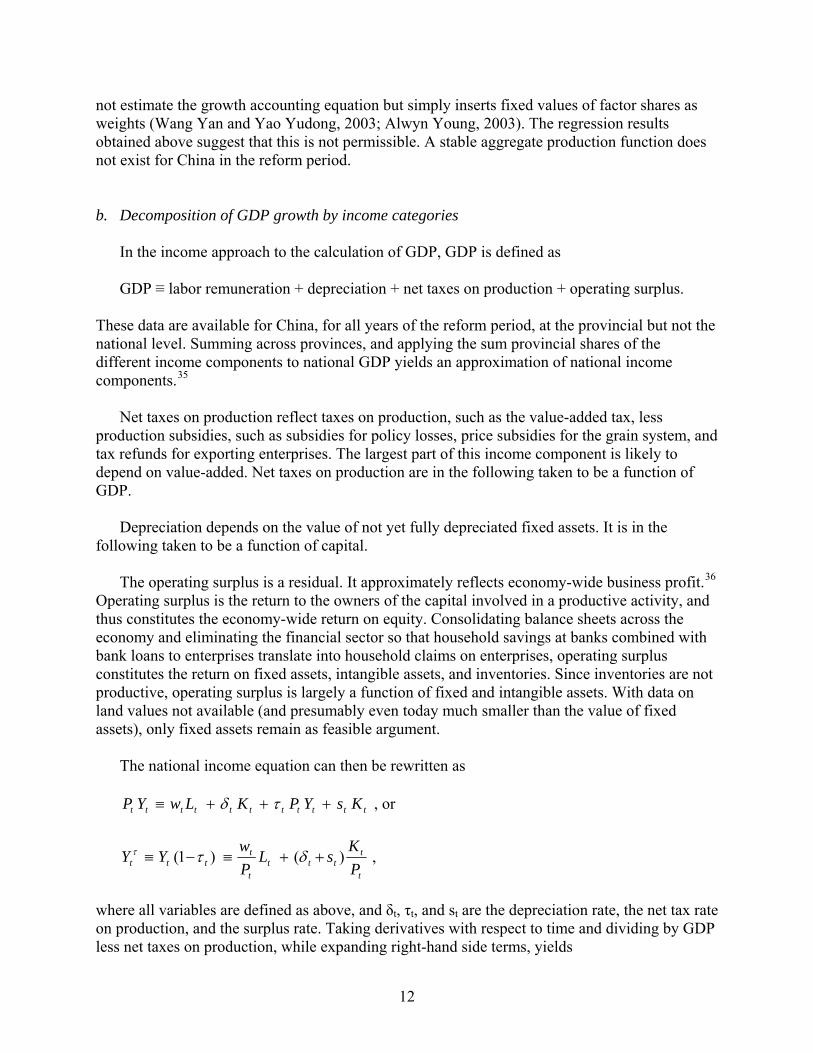
not estimate the growth accounting equation but simply inserts fixed values of factor shares as weights (Wang Yan and Yao Yudong, 2003; Alwyn Young, 2003). The regression results obtained above suggest that this is not permissible. A stable aggregate production function does not exist for China in the reform period. b. Decomposition of GDP growth by income categories In the income approach to the calculation of GDP, GDP is defined as GDP ≡ labor remuneration + depreciation + net taxes on production + operating surplus. These data are available for China, for all years of the reform period, at the provincial but not the national level. Summing across provinces, and applying the sum provincial shares of the different income components to national GDP yields an approximation of national income components.35 Net taxes on production reflect taxes on production, such as the value-added tax, less production subsidies, such as subsidies for policy losses, price subsidies for the grain system, and tax refunds for exporting enterprises. The largest part of this income component is likely to depend on value-added. Net taxes on production are in the following taken to be a function of GDP. Depreciation depends on the value of not yet fully depreciated fixed assets. It is in the following taken to be a function of capital. The operating surplus is a residual. It approximately reflects economy-wide business profit.36 Operating surplus is the return to the owners of the capital involved in a productive activity, and thus constitutes the economy-wide return on equity. Consolidating balance sheets across the economy and eliminating the financial sector so that household savings at banks combined with bank loans to enterprises translate into household claims on enterprises, operating surplus constitutes the return on fixed assets, intangible assets, and inventories. Since inventories are not productive, operating surplus is largely a function of fixed and intangible assets. With data on land values not available (and presumably even today much smaller than the value of fixed assets), only fixed assets remain as feasible argument. The national income equation can then be rewritten as

ttttttttttt KsYPKLwYP +++≡ τδ , or

t

tttt

t

tttt P

KsL

Pw

YY )()1( ++≡−≡ δττ ,

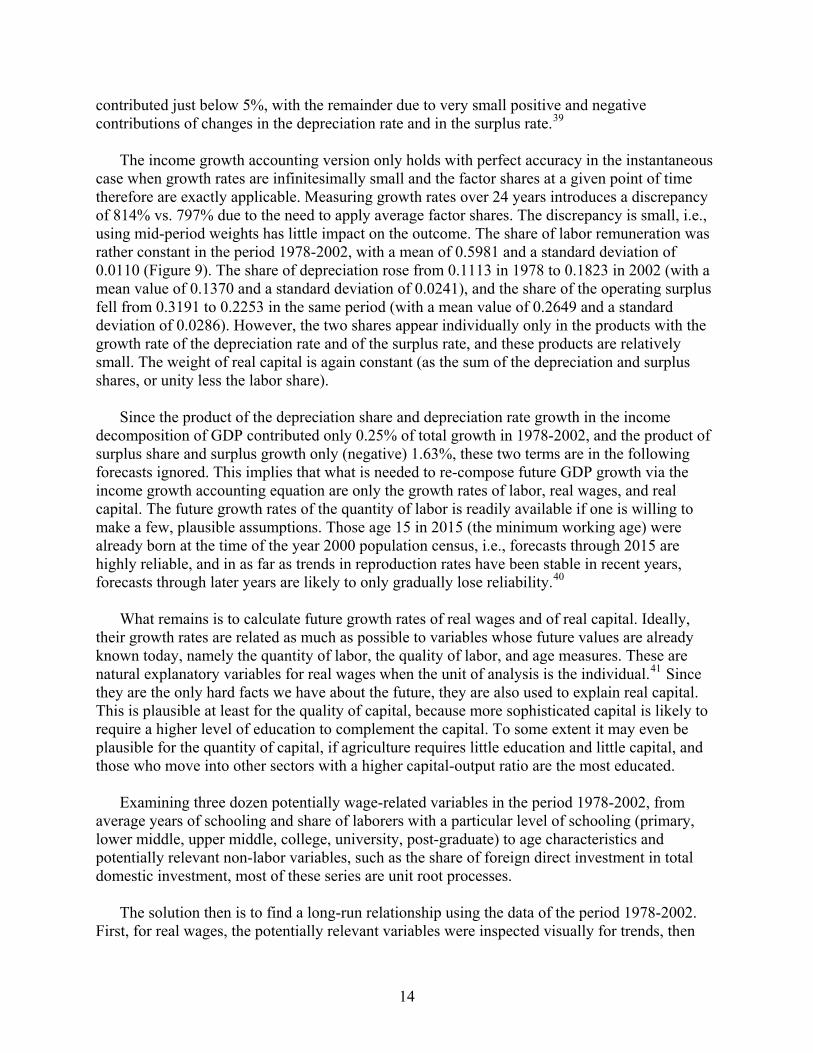
where all variables are defined as above, and δt, τt, and st are the depreciation rate, the net tax rate on production, and the surplus rate. Taking derivatives with respect to time and dividing by GDP less net taxes on production, while expanding right-hand side terms, yields

12

)1()1(

)1(

tt

tt

tt

tt

t

t

Ydt

dY

Ydt

dY

Ydt

dY

τ

τ

τ

ττ

τ

−−

−

−≡

τττττ δδ

δ

δ

t

t

t

t

t

t

t

ttt

t

t

t

t

t

t

t

t

t

t

t

t

t

t

t

t

t

t

t

t

t

t

t

t

t

YPK

PKdtPK

d

sYs

PK

sdtds

YPKdt

d

Ldt

dL

YL

Pw

YPw

L

PwdtPw

d

)( +++++≡ .

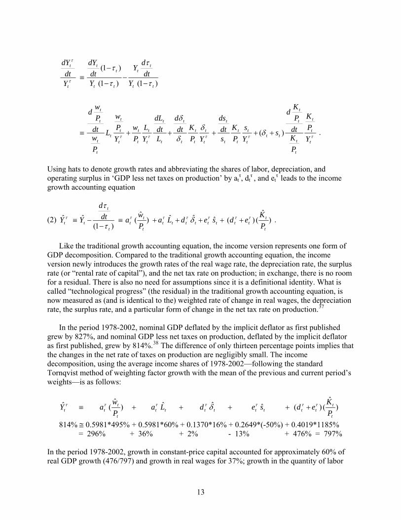
Using hats to denote growth rates and abbreviating the shares of labor, depreciation, and operating surplus in ‘GDP less net taxes on production’ by at

τ, dtτ , and et

τ leads to the income growth accounting equation

(2) )ˆ

()(ˆˆˆ)ˆ

()1(

ˆˆt

ttttttttt

t

tt

t

t

tt PK

edsedLaPw

adtd

YY τττττττ δτ

τ

+++++≡−

−≡ .

Like the traditional growth accounting equation, the income version represents one form of GDP decomposition. Compared to the traditional growth accounting equation, the income version newly introduces the growth rates of the real wage rate, the depreciation rate, the surplus rate (or “rental rate of capital”), and the net tax rate on production; in exchange, there is no room for a residual. There is also no need for assumptions since it is a definitional identity. What is called “technological progress” (the residual) in the traditional growth accounting equation, is now measured as (and is identical to the) weighted rate of change in real wages, the depreciation rate, the surplus rate, and a particular form of change in the net tax rate on production.37

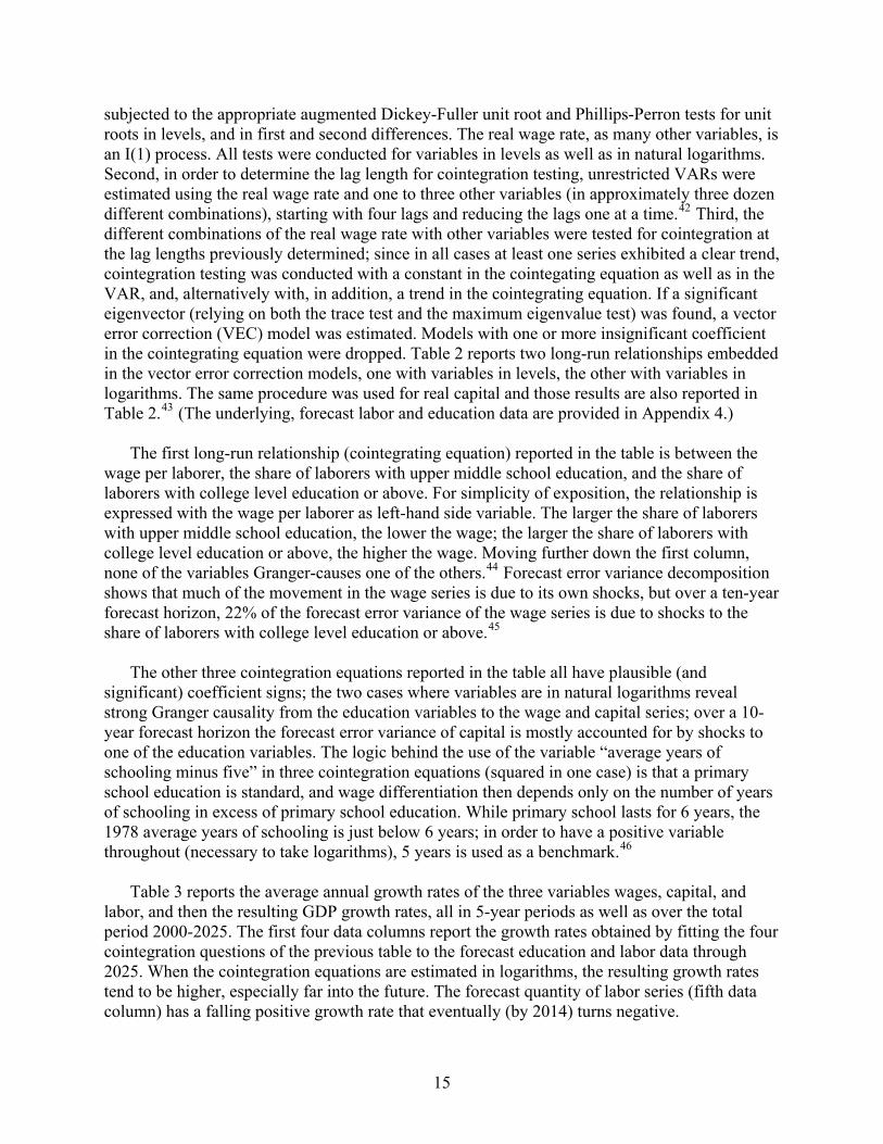
In the period 1978-2002, nominal GDP deflated by the implicit deflator as first published grew by 827%, and nominal GDP less net taxes on production, deflated by the implicit deflator as first published, grew by 814%.38 The difference of only thirteen percentage points implies that the changes in the net rate of taxes on production are negligibly small. The income decomposition, using the average income shares of 1978-2002—following the standard Tornqvist method of weighting factor growth with the mean of the previous and current period’s weights—is as follows:

)ˆ

()(ˆˆˆ)ˆ

(ˆt

ttttttttt

t

ttt P

KedsedLa

Pw

aY τττττττ δ +++++≡

814% ≅ 0.5981*495% + 0.5981*60% + 0.1370*16% + 0.2649*(-50%) + 0.4019*1185% = 296% + 36% + 2% - 13% + 476% = 797%

In the period 1978-2002, growth in constant-price capital accounted for approximately 60% of real GDP growth (476/797) and growth in real wages for 37%; growth in the quantity of labor

13

contributed just below 5%, with the remainder due to very small positive and negative contributions of changes in the depreciation rate and in the surplus rate.39 The income growth accounting version only holds with perfect accuracy in the instantaneous case when growth rates are infinitesimally small and the factor shares at a given point of time therefore are exactly applicable. Measuring growth rates over 24 years introduces a discrepancy of 814% vs. 797% due to the need to apply average factor shares. The discrepancy is small, i.e., using mid-period weights has little impact on the outcome. The share of labor remuneration was rather constant in the period 1978-2002, with a mean of 0.5981 and a standard deviation of 0.0110 (Figure 9). The share of depreciation rose from 0.1113 in 1978 to 0.1823 in 2002 (with a mean value of 0.1370 and a standard deviation of 0.0241), and the share of the operating surplus fell from 0.3191 to 0.2253 in the same period (with a mean value of 0.2649 and a standard deviation of 0.0286). However, the two shares appear individually only in the products with the growth rate of the depreciation rate and of the surplus rate, and these products are relatively small. The weight of real capital is again constant (as the sum of the depreciation and surplus shares, or unity less the labor share). Since the product of the depreciation share and depreciation rate growth in the income decomposition of GDP contributed only 0.25% of total growth in 1978-2002, and the product of surplus share and surplus growth only (negative) 1.63%, these two terms are in the following forecasts ignored. This implies that what is needed to re-compose future GDP growth via the income growth accounting equation are only the growth rates of labor, real wages, and real capital. The future growth rates of the quantity of labor is readily available if one is willing to make a few, plausible assumptions. Those age 15 in 2015 (the minimum working age) were already born at the time of the year 2000 population census, i.e., forecasts through 2015 are highly reliable, and in as far as trends in reproduction rates have been stable in recent years, forecasts through later years are likely to only gradually lose reliability.40 What remains is to calculate future growth rates of real wages and of real capital. Ideally, their growth rates are related as much as possible to variables whose future values are already known today, namely the quantity of labor, the quality of labor, and age measures. These are natural explanatory variables for real wages when the unit of analysis is the individual.41 Since they are the only hard facts we have about the future, they are also used to explain real capital. This is plausible at least for the quality of capital, because more sophisticated capital is likely to require a higher level of education to complement the capital. To some extent it may even be plausible for the quantity of capital, if agriculture requires little education and little capital, and those who move into other sectors with a higher capital-output ratio are the most educated. Examining three dozen potentially wage-related variables in the period 1978-2002, from average years of schooling and share of laborers with a particular level of schooling (primary, lower middle, upper middle, college, university, post-graduate) to age characteristics and potentially relevant non-labor variables, such as the share of foreign direct investment in total domestic investment, most of these series are unit root processes. The solution then is to find a long-run relationship using the data of the period 1978-2002. First, for real wages, the potentially relevant variables were inspected visually for trends, then

14

subjected to the appropriate augmented Dickey-Fuller unit root and Phillips-Perron tests for unit roots in levels, and in first and second differences. The real wage rate, as many other variables, is an I(1) process. All tests were conducted for variables in levels as well as in natural logarithms. Second, in order to determine the lag length for cointegration testing, unrestricted VARs were estimated using the real wage rate and one to three other variables (in approximately three dozen different combinations), starting with four lags and reducing the lags one at a time.42 Third, the different combinations of the real wage rate with other variables were tested for cointegration at the lag lengths previously determined; since in all cases at least one series exhibited a clear trend, cointegration testing was conducted with a constant in the cointegating equation as well as in the VAR, and, alternatively with, in addition, a trend in the cointegrating equation. If a significant eigenvector (relying on both the trace test and the maximum eigenvalue test) was found, a vector error correction (VEC) model was estimated. Models with one or more insignificant coefficient in the cointegrating equation were dropped. Table 2 reports two long-run relationships embedded in the vector error correction models, one with variables in levels, the other with variables in logarithms. The same procedure was used for real capital and those results are also reported in Table 2.43 (The underlying, forecast labor and education data are provided in Appendix 4.) The first long-run relationship (cointegrating equation) reported in the table is between the wage per laborer, the share of laborers with upper middle school education, and the share of laborers with college level education or above. For simplicity of exposition, the relationship is expressed with the wage per laborer as left-hand side variable. The larger the share of laborers with upper middle school education, the lower the wage; the larger the share of laborers with college level education or above, the higher the wage. Moving further down the first column, none of the variables Granger-causes one of the others.44 Forecast error variance decomposition shows that much of the movement in the wage series is due to its own shocks, but over a ten-year forecast horizon, 22% of the forecast error variance of the wage series is due to shocks to the share of laborers with college level education or above.45 The other three cointegration equations reported in the table all have plausible (and significant) coefficient signs; the two cases where variables are in natural logarithms reveal strong Granger causality from the education variables to the wage and capital series; over a 10-year forecast horizon the forecast error variance of capital is mostly accounted for by shocks to one of the education variables. The logic behind the use of the variable “average years of schooling minus five” in three cointegration equations (squared in one case) is that a primary school education is standard, and wage differentiation then depends only on the number of years of schooling in excess of primary school education. While primary school lasts for 6 years, the 1978 average years of schooling is just below 6 years; in order to have a positive variable throughout (necessary to take logarithms), 5 years is used as a benchmark.46 Table 3 reports the average annual growth rates of the three variables wages, capital, and labor, and then the resulting GDP growth rates, all in 5-year periods as well as over the total period 2000-2025. The first four data columns report the growth rates obtained by fitting the four cointegration questions of the previous table to the forecast education and labor data through 2025. When the cointegration equations are estimated in logarithms, the resulting growth rates tend to be higher, especially far into the future. The forecast quantity of labor series (fifth data column) has a falling positive growth rate that eventually (by 2014) turns negative.

15

Assuming a constant depreciation rate, surplus rate, and net tax rate on production (as the decomposition for the period 1978-2002 suggests is permissible), future GDP growth can be obtained by summing the growth rates of wages, capital, and labor; in each year, the weights, in form of the tax-adjusted labor share and one minus this share, are the previous-year values (for details see notes to the table). Depending on if the cointegration equation using variables in levels or in logarithms is used, the resulting average annual GDP growth rate of the period 2000-05 is 5.80 or 8.09% (sixth and seventh data columns in the table). With actual real growth in this period likely to be between 8 and 9%, the second series, with the cointegration based on variables in logarithms, seems to be more accurate.47 In the periods 2005-10 and 2010-25, the two series yield rather similar estimates, in the range of 7.05-9.42%. At this level of economic growth, the extrapolations of Table 1 suggest that China will surpass the U.S. economy in size, using the purchasing power concept, around the middle of the next decade. Further into the future, the predictions diverge significantly, with one GDP growth series falling off, and the other rising. Due to the recent explosion in education, the out-of-sample forecasts use education values that are far from sample average values. As the educational level of laborers increases, the marginal product of education could fall, and the predicted values then constitute an overestimate; on the other hand, if labor is increasingly paid its marginal product value rather than state-ordained wages, the predicted values constitute an underestimate. The comparison of the two GDP growth series shows well the degree of uncertainty involved in predicting further into the future than 2015. The two series reflect extreme scenarios. A different combination of wage and capital series yields intermediate growth values. An alternative approach to predicting GDP growth is to assume a constant labor share. This is plausible given worldwide experiences. Figure 10 shows that it is also plausible given past labor share values in China (now labor share in GDP, not in GDP less net taxes on production). Given the definition of the labor share as labor remuneration divided by GDP, and, if dividing numerator and denominator by the price level, as

t

tt

t

t Y

LPw

a ≡ ,

and assuming the labor share at to be constant, yields the growth rate of real GDP as

tt

tt L

Pw

Y ˆˆˆ +≡ .

I.e., real GDP growth is simply the sum of real wage growth and labor growth.48 Data on future labor growth through approximately 2025 are available. Real wage growth is plausibly explained by the quantity and quality of labor. The relationship for the period 1978-2002 was identified above and can be applied to the reliable data on the future quantity and quality of labor available through approximately 2025. This procedure by-passes the need for a capital series. Table 3 in the last two columns reports the results. They carry no new or different insights but confirm the findings following the more elaborate decomposition of GDP growth by income categories.

16

The growth forecasts use only facts about the future quantity and quality of laborers in China that are near-certain today. With little change in China’s labor force over the next twenty years, economic growth depends on growth in the wage rate and, in the decomposition of GDP growth by income categories, the accumulation of physical capital. The time series estimations established a long-run relationship of both variables to human capital and labor data, with the relationships then applied to future human capital and labor data. The next section explores in more detail the most recent developments in human capital formation in China.

5. Human Capital

Growth in human capital in reform period China has been rapid. A comparison with the U.S. puts China’s human capital measures into perspective, while the development of education in China over time reveals the scale of changes underway. Table 4 compares the educational level of the Chinese vs. U.S. population as reported in the population censuses of 1990 and 2000 in both countries.49 As a percentage of the total population, a far higher proportion of the U.S. population has achieved a secondary or tertiary level of education. For example, in 1990, 75.2% of the U.S. population had completed high school, but only 9.52% of the Chinese population had; 20.3% of the U.S. population had completed a bachelor’s degree (or above), but only 0.56% of the Chinese population had. But because the U.S. population in 1990 was only 28% of the size of the Chinese population (in 2000, 24%), the difference shrinks by a factor of approximately four once total population numbers are considered. Between 1990 and 2000, China narrowed the relative gap. While in 1990 the number of U.S. citizens with high school education was 1.65 times the number in China, by 2000 this ratio had fallen to 1.17 (last column in Table 4). For the BA degree, the ratio fell from 7.59 to 4.33. At the level above the bachelor’s degree the ratio in 2000 was still 21.42 in favor of the U.S. (with no such figure available for 1990). These data cover the population in total. But the educational level of different age cohorts in China is changing rapidly over time. Figure 11 shows that in 2000 more than half the population age 65 or above had a level of education below primary school; only 10.55% had some form of secondary education (lower or upper middle-school), and 1.50% had a tertiary level education. In contrast, in the age cohort 20-29 years, only 2.06% had a level of education below primary school, 20.98% completed only primary school, 69.44% achieved some form of secondary education, and 7.53% obtained a tertiary level education. The age cohorts in between reveal a smooth transition from the less educated older generation to the ever better educated younger age cohorts.50 At the primary and secondary school level, the Chinese age cohort 20-29 years in 2000 comes close to the U.S. population average level, but in tertiary education still falls far short. Current-year new enrollment data at the tertiary level reveal that at the BA level (including college-level associate degrees) China has caught up with the U.S. Figure 12 shows new enrollment numbers in Chinese BA programs, in contrast to the U.S. In the reform period, new

17

enrollment in China first languished, but began to expand gradually in the early 1980s and then rapidly after 1998. In 1998, new enrollment was at approximately twice its 1978 level. But then, in the course of just 5 years, between 1998 and 2003, new enrollment almost quadrupled. Since 2001, the absolute new enrollment number in Chinese BA programs at (only) regular institutions of higher education exceeds the number of freshmen in the U.S. China’s preliminary figure on new enrollment at regular institutions of higher education for 2004 is 4.473m, and the projection for 2005 is 4.75m.51 If U.S. new enrollment numbers continue to be stable over time (Figure 12), new enrollment in China is currently twice the U.S. figure. Data on the joint category of MA and PhD new enrollment in China (also Figure 12) follow the same trend as new enrollment for the BA/ college-level associate degree. Lacking data on new enrollment at the graduate level in the U.S., and therefore assuming that the past graduation number of 400-500,000 MA and PhD degree holders is an accurate indicator of current new enrollment, U.S. enrollment numbers at the graduate level were five times the Chinese figure in 1999, but only 1/3 above the Chinese figure in 2004. With new enrollment at the tertiary level rising drastically in recent years, so does the number of graduates (Figure 13). The absolute number of undergraduate level graduates in China came within hair-width of that in the U.S. in 2003.52 If students newly enrolled in 1999/2000 graduated in 2003 (3-4 years later), then the number of graduates in 2007 should be about three times larger than in 2003. Because U.S. enrollment numbers have risen only marginally in recent years, the number of undergraduate degrees awarded in China in 2007 will then be more than twice the number in the U.S. At the MA and PhD level (with only joint data available for China), the U.S. in 2003 still had a 5-fold lead in absolute graduation numbers (Figure 13 and Table 5).53 But with U.S. graduate numbers stable, Chinese enrollment rates of 2003, assuming no drop-outs, imply that the gap will narrow to a barely 2-fold lead for the U.S. by 2006, while 2004 enrollment numbers suggest a less than 1.5-fold lead for the U.S. in 2007.54

At the high school level, the number of Chinese graduates has well exceeded their U.S. counterpart in absolute numbers throughout the reform period. In 2003, China had 2.48 times more high school graduates than the U.S. (Table 5).55 The price of education in China has been rising rapidly. Supposedly strict limits on fees levied on compulsory education suggest that much of the price increase reflects demand for senior high school and tertiary level education. Between 1988 (the earliest year for an uninterrupted time series through today) and 2003, the consumer price index (CPI) rose by an average of 6.20.% per year. But its subindex “tuition and child care” rose by an average of 20.05% per year, i.e., almost four times faster than the CPI (Figure 14).56 The difference in price increases was largest in the late 1990s, despite the at this time drastic increase in new enrollment at regular institutions of higher education, where at least admission to the BA, if not to the college-level associate degree, is government controlled. Only in 2002 and 2003 has the difference in price increases narrowed to a few percentage points, which could suggest that demand is finally leveling off (unless price caps were imposed by the government).

18

Head count data do not necessarily translate into comparable accumulation of human capital since they reveal nothing about the quality of education.57 But it is not at all certain that education in China through the secondary school level is necessarily inferior to that in the U.S. Even at the tertiary level, a provincial railway ministry college in China need not be inferior to a U.S. community college. At the top range of tertiary education, the conclusion is likely to be far less ambiguous; at that level, Chinese students seem to make good use of U.S. institutions. The explosion in education is only happening since the late 1990s. Much of the upgrading in the education level of Chinese laborers will not be felt until some years later. This again implies a fair amount of uncertainty about where exactly China’s economy will be by 2025. Not all the additional graduates are likely to be as qualified as the average graduate of earlier generations. On the other hand, with current private returns to education possibly far below the marginal product value, further reforms could mean a more important role for education in economic growth in the future. 6. Conclusions and Implications

Extrapolation into the future of China’s reform period economic growth suggests that the size of China’s economy will exceed that of the U.S., in purchasing power parity terms, in less than ten years. Per capita, the point of time when China catches up with the U.S. is much further into the future, thirty to forty years from now, although the coastal areas, especially the in the past fastest growing five provinces together with Shanghai, with a population exceeding that of the U.S., may catch up in as little as two decades.

China’s economic development in the reform period fits well with the broad development

patterns of structural change, catching up, and factor price equalization, not least in comparison with other Asian countries earlier in their economic development. On all accounts, China has twenty to forty more years of gains in economic growth to reap. Re-composing China’s economic growth from growth in income components suggests that China’s continued growth is inevitable. Based on the year 2000 population census combined with past and current trends in education, the quantity and quality of China’s laborers can be predicted with near-certainty through 2015, and with high reliability for the years after. These forecasts suggest economic growth between 2005 and 2015 in the range of 7-9%, high enough for China to catch up with the U.S., in purchasing power terms, within a decade or less.

Growth accounting illustrates the correlation between (and potential impact of) changes in the educational structure of China’s population and (on) economic growth. China’s population is four times the size of the U.S. population. If talent is randomly distributed among the world population and if China’s education system is able to identify the brightest students, then China has a larger pool of talent to draw from than any other country in the world.58 If innovation depends on the agglomeration of talent (geographically, nationally, culturally, or linguistically), then China is in an excellent position to grow and innovate.59

Demographics also matters in terms of market size (and 80% of China’s population lives in the densely populated Eastern part of the country). Size of the domestic market should allow

19

unprecedented variety and economies of scale. It is likely to have a positive impact on competition and, thereby, rationalization and innovation. The large pool of laborers, compared to other countries, could in time lead to a highly efficient allocation of labor in that each labor market niche can be filled by the appropriate talent.

Domestically, China’s continued economic growth means that one-fifth of the world population will continue to experience significant improvements in their living standard. A share of China’s population that exceeds the size of the U.S. population will enjoy living standards close to the level of developed countries in the near future. Others will rise out of poverty, while the sweatshops of early industrialization disappear sooner rather than later. Internationally, China’s economic growth will continue to affect relative prices and production structures around the world. China’s trade volume is exceptionally large by international standards. In 2000, China’s ratio of ‘exports of goods and services’ to GDP was 25.90%, compared to 11.21% for the U.S.60 By 2003, China’s ratio of exports of goods and services to GDP at 34.24% was almost ten percentage points higher (while imports stood at 31.69%).61 Even if this ratio only stays constant in the future rather than rises further, China’s economic growth means that China will soon be the world’s largest exporter and importer.

While some in the West fret about the “China price” and its impact on Western economies,

some firms in Western economies will benefit from the increasing division of labor, as will those who have a stake in these firms (for example, the typical pension fund of citizens of Western countries). Two-thirds of China’s imports originate in Asia (where it sends half of its exports). China’s economic growth, therefore, induces economic growth in other Asian countries. India may be tempted by China’s example into sustained, growth-promoting economic reforms. It appears only a matter of time (ten years?) before the center of world economic activity, as measured by GDP, shifts to Asia. These developments appear little different from the economic rise of other nations in the past, except perhaps the speed at which they occur, and the breadth of implications due to the size of China. But what may cause particular discomfort in the West is the fact that China is, following its Constitution, a “people’s democratic dictatorship ... under the leadership of the Communist Party of China.” As China’s FDI abroad grows, political questions may become more pressing, such as to what extent Chinese investors abroad are simply extensions of the Politburo (which appoints the managers of 53 of the largest state-owned enterprises), or to what extent the world plays by the rules of China’s dictator(s) a few years down the road? But the influence goes both ways. In 2003, 16.48% of value-added in industrial enterprises with annual sales revenue in excess of 5m yuan RMB (USD 0.6m) within China was produced by foreign-funded enterprises, a figure which excludes an additional 11.15% in enterprises funded by Hong Kong, Macau, and Taiwanese entrepreneurs.62 For years to come, China is likely to want to enjoy the benefits of access to foreign capital and foreign technology. China is adopting international standards and practices on a scale and at a speed as perhaps no other county in the world ever has. A larger share of China’s bureaucrats and enterprise managers are likely to have a foreign education or work experience abroad than in Western countries. On many measures, China is an extremely open economy.

20

China’s rapid economic rise is not guaranteed. Economic problems range from bad loans in the banking system to an under-funded pension insurance scheme, the lack of a rural health care system, and bankrupt local governments. Yet China’s leadership has a track record spanning more than two decades of rising to economic challenges and addressing problems as they become urgent. At a 9.37% average annual real growth rate, furthermore, GDP doubles every eight years; if the absolute size of a financial deficit stays constant during this period, its significance, as a share of GDP, is halved. This provides all the more reason for China’s leadership to stay focused on economic growth. Economic growth also does not necessarily come with the connotation “good.” Much of GDP growth could be accompanied by significant environmental degradation and resource exhaustion. A “green GDP” growth rate could be several percentage points lower.63 At some point, China’s leadership may no longer wish to trade off China’s environment and resources for GDP growth. But even once that happens, it is likely to be a gradual process. Political constraints may yet pose greater constraints on China’s economic growth than economic or financial imbalances. Growing inequality or increasing dissatisfaction with widespread government/Party corruption could lead to a breakdown of political governance in China. From a more continuous perspective, China’s severe control over access to information is unlikely to advance economic growth. At least social scientists work within a framework of relatively scarce information; information is more freely available only to those who are part of internal circles. Consequently, public scientific discourse is limited and a significant Chinese language research community centered around Chinese language research publications has yet to emerge. When China’s economy is ready to move from catching up to innovation on a larger scale, these information constraints are unlikely to be helpful. A second aspect is the Party’s control over key appointments across the economy, from state-owned enterprises to the banking system (and, naturally, all leadership positions in government). The consequences of the appointment of, when in doubt, “red” rather than professional managers, and the absence of effective control mechanisms is unlikely to be conducive to economic growth and efficiency; evidence in form of corruption scandals abounds. These political constraints not only threaten to have a direct impact on the operation of China’s economy, but are also likely to continue to induce some of the best Chinese-born talents to move or stay abroad.

21

References Chinese names in pinyin form are given last name first, followed by first name, without comma

in between. Abramovitz, Moses. “Catching Up, Forging Ahead, and Falling Behind.” Journal of Economic

History 46, no. 2 (June 1986): 385-406. Annual Report on National Income Statistics. Economic Planning Agency, Government of Japan;

various issues. Barro, Robert J., and Xavier Sala-i-Martin. Economic Growth. New York: McGraw-Hill, 1995. Broomfield, Emma V. “Perceptions of Danger: the China Threat Theory.” Journal of

Contemporary China 12, no. 35 (2003): 265-84. Brown, Lester Russell. Who Will Feed China? Wake-up Call for a Small Planet. New York :

W.W. Norton & Co., 1995. Carter, Colin A., and Scott Rozelle. “Will China Become a Major Force in World Food

Markets?” Review of Agricultural Economics 23, no. 2 (Fall-Winter 2001): 319-31. Census 1990. Zhongguo 1990 nian quanguo renkou pucha ziliao (National population census

material 1990). Compiled by the State Council population census office and the NBS population division. Beijing: Zhongguo tongji chubanshe, 1993.

Census 2000. Zhongguo 2000 nian quanguo renkou pucha ziliao (National population census material 2000). Compiled by the State Council population census office and the NBS population, society, and science division. Beijing: Zhongguo tongji chubanshe, 2002.

Census 2000 Major Figures. 2000 nian di wu ci quanguo renkou pucha zhuyao shuju (Major figures from the 2000 population census of China). Beijing: Zhongguo tongji chubanshe, 2001.

Census 2000 (nationality). 2000 nian renkou pucha zhongguo minzu renkou ziliao (National population census material 2000 by nationality). Issued by the NBS population, society, and science division. Beijing: Zhongguo tongji chubanshe, 2003.

Chang, Gordon G. The Coming Collapse of China. New York: Random House, 2001. Chow, Gregory C. “Capital Formation and Economic Growth in China.” The Quarterly Journal

of Economics 108, no. 3 (Aug. 1993): 809-42. _____. China’s Economic Transformation. Malden, MA: Blackwell Publishing, 2002. Chow, Gregory, and Kui-Wai Li. “China’s Economic Growth 1952-2010.” Economic

Development and Cultural Change 51, no. 1 (Oct. 2002): 247-56. Cypher, James M., and James L. Dietz. The Process of Economic Development. London:

Routledge, 1997. Douglas, Allen. “Meet the New China.” International Journal of Business 7, no. 3 (2002): 35-49. Education Yearbook. Zhongguo jiaoyu nianjian (China Education Yearbook). Beijing: Zhongguo

jiaoyu chubanshe, annual publication. Educational Attainment 2000. At http://www.census.gov/prod/2003pubs/c2kbr-24.pdf, accessed

on 1 January 2004. Felipe, Jesus, and Carsten A. Holz. “Why Do Aggregate Production Functions Work? Fisher’s

Simulations, Shaikh’s Identity and Some New Results.” International Review of Applied Economics 15, no. 3 (2001): 261-85.

22

Fifty Years of New China. Xin zhongguo wushi nian tongji ziliao huibian (Compendium of Statistical Materials for the Fifty Years of New China). Beijing: Zhongguo tongji chubanshe, 1999.

Financial Yearbook. Zhongguo jinrong nianjian (China Financial Yearbook). Beijing: Zhongguo jinrong chubanshe, numerous issues.

GDP 1952-95. Zhongguo guonei shengchan zongzhi hesuan lishi ziliao 1952-1995 (Historical Data on China's Gross Domestic Product 1952-1995). Dalian: Dongbei caijing daxue chubanshe, 1997.

GDP 1996-2002. Zhongguo guonei shengchan zongzhi hesuan lishi ziliao 1996-2002 (Historical Data on China's Gross Domestic Product 1996-2002). Beijing: Zhongguo tongji chubanshe, 2004.

Gertz, Bill. The China Threat: How the People’s Republic Targets America.” Washington, D.C.: Regnery Publishing, 2000.

Harberger, Arnold C. “A Vision of the Growth Process.” American Economic Review 88, no. 1 (March 1998): 1-32.

Heckman, James J. “China’s Human Capital Investment.” China Economic Review 16, no. 1 (2005): 50-70.

Henderson, Callum. China on the Brink: The Myths and Realities of the World’s Largest Market. New York: McGraw-Hill, 1999.

Heston, Alan. “Treatment of China in PWT 6.” Draft, December 2001. At http://pwt.econ.upenn.edu/Documentation/China.PDF, accessed on 16 Dec. 2003.

Heston, Alan, Daniel A. Nuxoll, and Robert Summers. “Comparative Country Performance at Own-Prices or Common International Prices,” in M. Dutta (ed.), Economics, Econometrics and the Link: Essays in Honor of Lawrence R. Klein. Amsterdam: Elsevier, 1995, pp. 345-61.

Holz, Carsten A. China’s Industrial State-owned Enterprises: Between Profitability and Bankruptcy. Singapore: World Scientific Publishing Co., 2003.

_____. “New Capital Estimates for China.” Mimeo, Hong Kong University of Science & Technology, March 2005(a), at http://ihome.ust.hk/~socholz.

_____. “The Quantity and Quality of Labor in China 1978-2000-2025.” Mimeo, Hong Kong University of Science & Technology, May 2005(b), at http://ihome.ust.hk/~socholz.

_____. “China’s Reform Period Economic Growth: How Reliable Are Angus Maddison’s Estimates?” Forthcoming in the Review of Income and Wealth, 2005(c).

IFS. International Financial Statistics Yearbook. Washington, D.C.: International Monetary Fund, various years.

Japan Statistical Yearbook 2004. Statistics Bureau/ Statistical Research and Training Institute, Ministry of Public Management, Home Affairs, Posts and Telecommunications.

Klein, Lawrence R., and Suleyman Ozmucur. “The Estimation of China’s Economic Growth Rate.” Mimeo, Department of Economics, University of Pennsylvania, 2003.

Lardy, Nicholas R. China’s Unfinished Economic Revolution. Washington, D.C.: The Brookings Institution, 1998.

Lin, Justin Yifu, Cai Fang, and Li Zhou. The China Miracle: Development Strategy and Economic Reform. Revised edition. Hong Kong: The Chinese University Press, 2003.

Murray, Geoffrey. China: The Next Superpower. Dilemmas in Change and Continuity. Richmond, Surrey: China Library (Curzon Press), 1998.

Nadiri, M. Ishaq. “Some Approaches to the Theory and Measurement of Total Factor Productivity: A Survey.” Journal of Economic Literature 8, no. 4 (Dec. 1970): 1137-77.

23

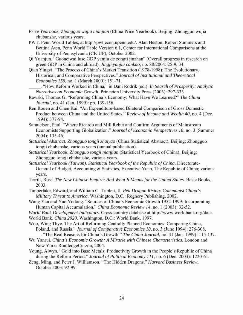
Price Yearbook. Zhongguo wujia nianjian (China Price Yearbook). Beijing: Zhongguo wujia chubanshe, various years.

PWT. Penn World Tables, at http://pwt.econ.upenn.edu/. Alan Heston, Robert Summers and Bettina Aten, Penn World Table Version 6.1, Center for International Comparisons at the University of Pennsylvania (CICUP), October 2002.

Qi Yuanjun. “Guoneiwai luse GDP yanjiu de zongti jinzhan” (Overall progress in research on green GDP in China and abroad). Jingji yanjiu cankao, no. 88/2004: 25-9, 34.

Qian Yingyi. “The Process of China’s Market Transition (1978-1998): The Evolutionary, Historical, and Comparative Perspectives.” Journal of Institutional and Theoretical Economics 156, no. 1 (March 2000): 151-71.

_____. “How Reform Worked in China,” in Dani Rodrik (ed.), In Search of Prosperity: Analytic Narratives on Economic Growth. Princeton University Press (2003): 297-333.

Rawski, Thomas G. “Reforming China’s Economy: What Have We Learned?” The China Journal, no. 41 (Jan. 1999): pp. 139-156.

Ren Rouen and Chen Kai. “An Expenditure-based Bilateral Comparison of Gross Domestic Product between China and the United States.” Review of Income and Wealth 40, no. 4 (Dec. 1994): 377-94.

Samuelson, Paul. “Where Ricardo and Mill Rebut and Confirm Arguments of Mainstream Economists Supporting Globalization.” Journal of Economic Perspectives 18, no. 3 (Summer 2004): 135-46.

Statistical Abstract. Zhongguo tongji zhaiyao (China Statistical Abstract). Beijing: Zhongguo tongji chubanshe, various years (annual publication).

Statistical Yearbook. Zhongguo tongji nianjian (Statistical Yearbook of China). Beijing: Zhongguo tongji chubanshe, various years.

Statistical Yearbook (Taiwan). Statistical Yearbook of the Republic of China. Directorate-General of Budget, Accounting & Statistics, Executive Yuan, The Republic of China; various years.

Terrill, Ross. The New Chinese Empire: And What It Means for the United States. Basic Books, 2003.

Timperlake, Edward, and William C. Triplett, II. Red Dragon Rising: Communist China’s Military Threat to America. Washington, D.C.: Regnery Publishing, 2002.

Wang Yan and Yao Yudong. “Sources of China’s Economic Growth 1952-1999: Incorporating Human Capital Accumulation.” China Economic Review 14, no. 1 (2003): 32-52.

World Bank Development Indicators. Cross-country database at http://www.worldbank.org/data. World Bank. China 2020. Washington, D.C.: World Bank, 1997. Woo, Wing Thye. The Art of Reforming Centrally Planned Economies: Comparing China,

Poland, and Russia.” Journal of Comparative Economics 18, no. 3 (June 1994): 276-308. _____. “The Real Reasons for China’s Growth.” The China Journal, no. 41 (Jan. 1999): 115-137. Wu Yanrui. China’s Economic Growth: A Miracle with Chinese Characteristics. London and

New York: RoutledgeCurzon, 2004. Young, Alwyn. “Gold into Base Metals: Productivity Growth in the People’s Republic of China

during the Reform Period.” Journal of Political Economy 111, no. 6 (Dec. 2003): 1220-61. Zeng, Ming, and Peter J. Williamson. “The Hidden Dragons.” Harvard Business Review,

October 2003: 92-99.

24

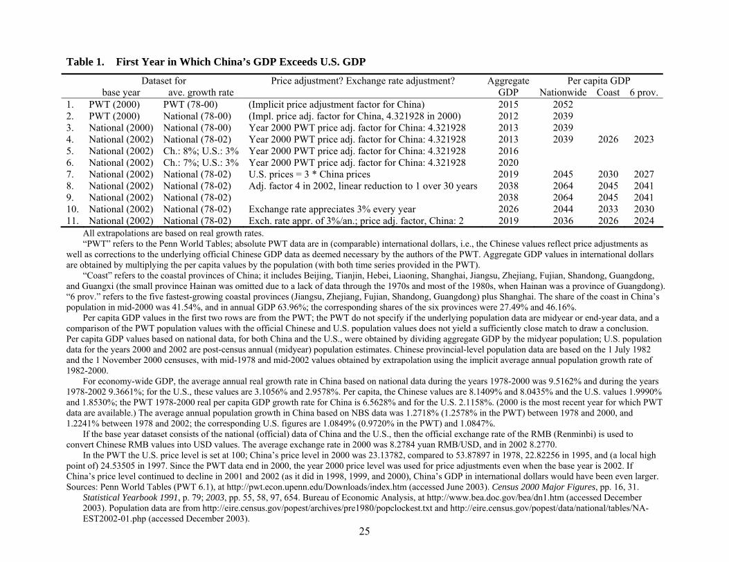
Table 1. First Year in Which China’s GDP Exceeds U.S. GDP

Dataset for Price adjustment? Exchange rate adjustment? Aggregate Per capita GDP base year ave. growth rate GDP Nationwide Coast 6 prov.

1. PWT (2000) PWT (78-00) (Implicit price adjustment factor for China) 2015 2052 2. PWT (2000) National (78-00) (Impl. price adj. factor for China, 4.321928 in 2000) 2012 2039 3. National (2000) National (78-00) Year 2000 PWT price adj. factor for China: 4.321928 2013 2039 4. National (2002) National (78-02) Year 2000 PWT price adj. factor for China: 4.321928 2013 2039 2026 2023 5. National (2002) Ch.: 8%; U.S.: 3% Year 2000 PWT price adj. factor for China: 4.321928 2016 6. National (2002) Ch.: 7%; U.S.: 3% Year 2000 PWT price adj. factor for China: 4.321928 2020 7. National (2002) National (78-02) U.S. prices = 3 * China prices 2019 2045 2030 2027 8. National (2002) National (78-02) Adj. factor 4 in 2002, linear reduction to 1 over 30 years 2038 2064 2045 2041 9. National (2002) National (78-02) 2038 2064 2045 2041 10. National (2002) National (78-02) Exchange rate appreciates 3% every year 2026 2044 2033 2030 11. National (2002) National (78-02) Exch. rate appr. of 3%/an.; price adj. factor, China: 2 2019 2036 2026 2024 All extrapolations are based on real growth rates. “PWT” refers to the Penn World Tables; absolute PWT data are in (comparable) international dollars, i.e., the Chinese values reflect price adjustments as well as corrections to the underlying official Chinese GDP data as deemed necessary by the authors of the PWT. Aggregate GDP values in international dollars are obtained by multiplying the per capita values by the population (with both time series provided in the PWT). “Coast” refers to the coastal provinces of China; it includes Beijing, Tianjin, Hebei, Liaoning, Shanghai, Jiangsu, Zhejiang, Fujian, Shandong, Guangdong, and Guangxi (the small province Hainan was omitted due to a lack of data through the 1970s and most of the 1980s, when Hainan was a province of Guangdong). “6 prov.” refers to the five fastest-growing coastal provinces (Jiangsu, Zhejiang, Fujian, Shandong, Guangdong) plus Shanghai. The share of the coast in China’s population in mid-2000 was 41.54%, and in annual GDP 63.96%; the corresponding shares of the six provinces were 27.49% and 46.16%. Per capita GDP values in the first two rows are from the PWT; the PWT do not specify if the underlying population data are midyear or end-year data, and a comparison of the PWT population values with the official Chinese and U.S. population values does not yield a sufficiently close match to draw a conclusion. Per capita GDP values based on national data, for both China and the U.S., were obtained by dividing aggregate GDP by the midyear population; U.S. population data for the years 2000 and 2002 are post-census annual (midyear) population estimates. Chinese provincial-level population data are based on the 1 July 1982 and the 1 November 2000 censuses, with mid-1978 and mid-2002 values obtained by extrapolation using the implicit average annual population growth rate of 1982-2000. For economy-wide GDP, the average annual real growth rate in China based on national data during the years 1978-2000 was 9.5162% and during the years 1978-2002 9.3661%; for the U.S., these values are 3.1056% and 2.9578%. Per capita, the Chinese values are 8.1409% and 8.0435% and the U.S. values 1.9990% and 1.8530%; the PWT 1978-2000 real per capita GDP growth rate for China is 6.5628% and for the U.S. 2.1158%. (2000 is the most recent year for which PWT data are available.) The average annual population growth in China based on NBS data was 1.2718% (1.2578% in the PWT) between 1978 and 2000, and 1.2241% between 1978 and 2002; the corresponding U.S. figures are 1.0849% (0.9720% in the PWT) and 1.0847%. If the base year dataset consists of the national (official) data of China and the U.S., then the official exchange rate of the RMB (Renminbi) is used to convert Chinese RMB values into USD values. The average exchange rate in 2000 was 8.2784 yuan RMB/USD, and in 2002 8.2770. In the PWT the U.S. price level is set at 100; China’s price level in 2000 was 23.13782, compared to 53.87897 in 1978, 22.82256 in 1995, and (a local high point of) 24.53505 in 1997. Since the PWT data end in 2000, the year 2000 price level was used for price adjustments even when the base year is 2002. If China’s price level continued to decline in 2001 and 2002 (as it did in 1998, 1999, and 2000), China’s GDP in international dollars would have been even larger.

25

Sources: Penn World Tables (PWT 6.1), at http://pwt.econ.upenn.edu/Downloads/index.htm (accessed June 2003). Census 2000 Major Figures, pp. 16, 31. Statistical Yearbook 1991, p. 79; 2003, pp. 55, 58, 97, 654. Bureau of Economic Analysis, at http://www.bea.doc.gov/bea/dn1.htm (accessed December 2003). Population data are from http://eire.census.gov/popest/archives/pre1980/popclockest.txt and http://eire.census.gov/popest/data/national/tables/NA-EST2002-01.php (accessed December 2003).

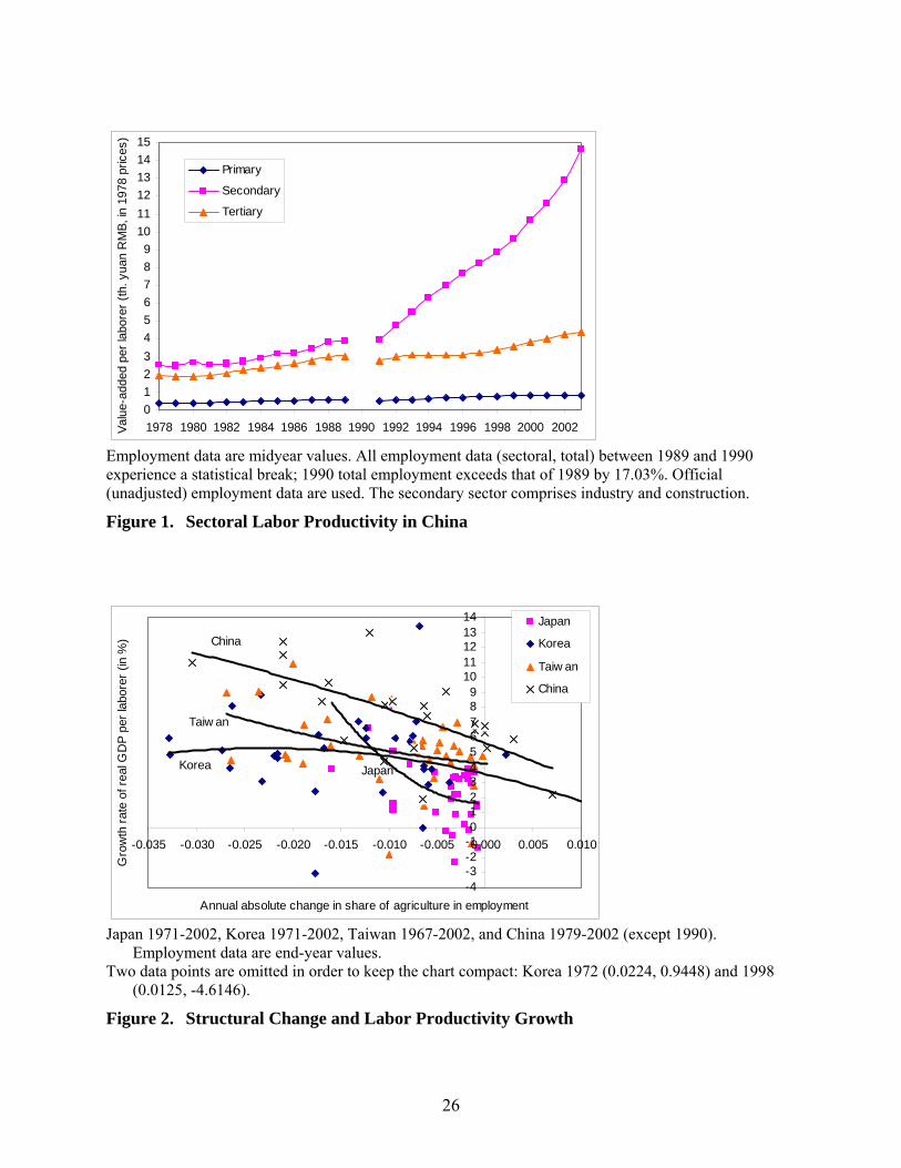
0123456789

101112131415

1978 1980 1982 1984 1986 1988 1990 1992 1994 1996 1998 2000 2002Valu

e-ad

ded

per l

abor

er (t

h. y

uan

RM

B, in

197

8 pr

ices

)

Primary

Secondary

Tertiary

Employment data are midyear values. All employment data (sectoral, total) between 1989 and 1990 experience a statistical break; 1990 total employment exceeds that of 1989 by 17.03%. Official (unadjusted) employment data are used. The secondary sector comprises industry and construction.

Figure 1. Sectoral Labor Productivity in China

-4-3-2-10123456789

1011121314

-0.035 -0.030 -0.025 -0.020 -0.015 -0.010 -0.005 0.000 0.005 0.010

Annual absolute change in share of agriculture in employment

Gro

wth

rate

of r

eal G

DP

per l

abor

er (i

n %

)

Japan

Korea

Taiw an

China

China

JapanKorea

Taiw an

Japan 1971-2002, Korea 1971-2002, Taiwan 1967-2002, and China 1979-2002 (except 1990).

Employment data are end-year values. Two data points are omitted in order to keep the chart compact: Korea 1972 (0.0224, 0.9448) and 1998

(0.0125, -4.6146).

Figure 2. Structural Change and Labor Productivity Growth

26

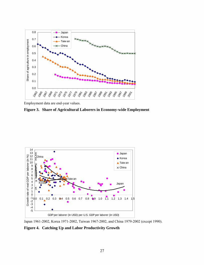
0.0

0.1

0.2

0.3

0.4

0.5

0.6

0.7

0.819

6319

6519

6719

6919

7119

7319

7519

7719

7919

8119

8319

8519

8719

8919

9119

9319

9519

9719

9920

01

Shar

e of

agr

icul

ture

in e

mpl

oym

ent

JapanKoreaTaiw anChina

Employment data are end-year values.

Figure 3. Share of Agricultural Laborers in Economy-wide Employment

-5-4-3-2-10123456789

1011121314

0.0 0.1 0.2 0.3 0.4 0.5 0.6 0.7 0.8 0.9 1.0 1.1 1.2 1.3 1.4 1.5

GDP per laborer (in USD) per U.S. GDP per laborer (in USD)

Gro

wth

rate

of r

eal G

DP

per l

abor

er (i

n %

) Japan

KoreaTaiw an

China

Japan

Taiw anKorea

China

Japan 1961-2002, Korea 1971-2002, Taiwan 1967-2002, and China 1979-2002 (except 1990).

Figure 4. Catching Up and Labor Productivity Growth

27

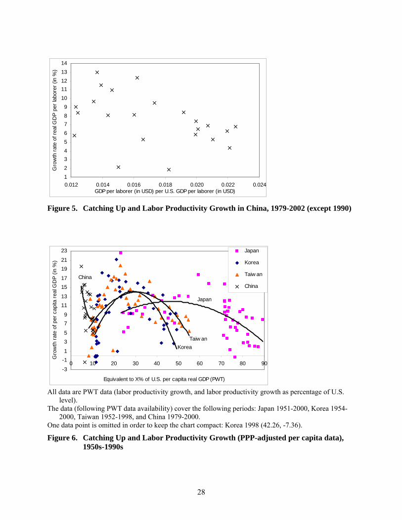
123456789

1011121314

0.012 0.014 0.016 0.018 0.020 0.022 0.024GDP per laborer (in USD) per U.S. GDP per laborer (in USD)

Gro

wth

rate

of r

eal G

DP

per l

abor

er (i

n %

)

Figure 5. Catching Up and Labor Productivity Growth in China, 1979-2002 (except 1990)

-3

-11

35

79

1113

1517

1921

23

0 10 20 30 40 50 60 70 80 9

Equivalent to X% of U.S. per capita real GDP (PWT)

Gro

wth

rate

of p

er c

apita

real

GD

P (in

%)

0

Japan

Korea

Taiw an

China

Japan

Taiw anKorea

China

All data are PWT data (labor productivity growth, and labor productivity growth as percentage of U.S.

level). The data (following PWT data availability) cover the following periods: Japan 1951-2000, Korea 1954-

2000, Taiwan 1952-1998, and China 1979-2000. One data point is omitted in order to keep the chart compact: Korea 1998 (42.26, -7.36).

Figure 6. Catching Up and Labor Productivity Growth (PPP-adjusted per capita data), 1950s-1990s

28

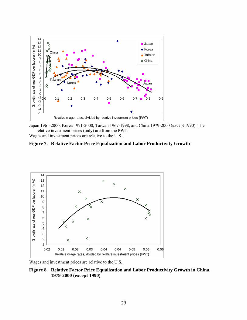
-5-4-3-2-10123456789

1011121314

0.0 0.1 0.2 0.3 0.4 0.5 0.6 0.7 0.8 0.9

Relative w age rates, divided by relative investment prices (PWT)

Gro

wth

rate

of r

eal G

DP

per l

abor

er (i

n %

) Japan

KoreaTaiw an

China

JapanTaiw an

Korea

China

Japan 1961-2000, Korea 1971-2000, Taiwan 1967-1998, and China 1979-2000 (except 1990). The

relative investment prices (only) are from the PWT. Wages and investment prices are relative to the U.S. Figure 7. Relative Factor Price Equalization and Labor Productivity Growth

123456789

1011121314

0.02 0.02 0.03 0.03 0.04 0.04 0.05 0.05 0.06Relative w age rates, divided by relative investment prices (PWT)

Gro

wth

rate

of r

eal G

DP

per l

abor

er (i

n %

)

Wages and investment prices are relative to the U.S. Figure 8. Relative Factor Price Equalization and Labor Productivity Growth in China,

1979-2000 (except 1990)

29

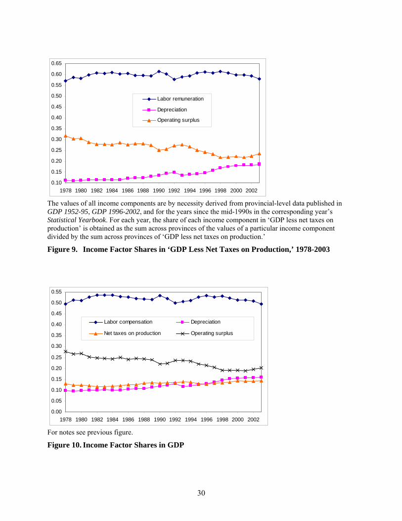
0.10

0.15

0.20

0.25

0.30

0.35

0.40

0.45

0.50

0.55

0.60

0.65

1978 1980 1982 1984 1986 1988 1990 1992 1994 1996 1998 2000 2002

Labor remuneration

Depreciation

Operating surplus

The values of all income components are by necessity derived from provincial-level data published in GDP 1952-95, GDP 1996-2002, and for the years since the mid-1990s in the corresponding year’s Statistical Yearbook. For each year, the share of each income component in ‘GDP less net taxes on production’ is obtained as the sum across provinces of the values of a particular income component divided by the sum across provinces of ‘GDP less net taxes on production.’

Figure 9. Income Factor Shares in ‘GDP Less Net Taxes on Production,’ 1978-2003

0.00

0.05

0.10

0.15

0.20

0.25

0.30

0.35

0.40

0.45

0.50

0.55

1978 1980 1982 1984 1986 1988 1990 1992 1994 1996 1998 2000 2002

Labor compensation Depreciation

Net taxes on production Operating surplus

For notes see previous figure.

Figure 10. Income Factor Shares in GDP

30

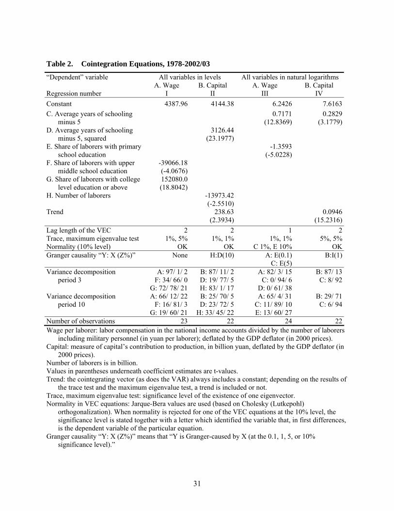
Table 2. Cointegration Equations, 1978-2002/03

“Dependent” variable All variables in levels All variables in natural logarithms A. Wage B. Capital A. Wage B. Capital Regression number I II III IV Constant 4387.96 4144.38 6.2426 7.6163C. Average years of schooling

minus 5 0.7171

(12.8369) 0.2829

(3.1779)D. Average years of schooling

minus 5, squared 3126.44

(23.1977)

E. Share of laborers with primary school education

-1.3593 (-5.0228)

F. Share of laborers with upper middle school education

-39066.18(-4.0676)

G. Share of laborers with college level education or above

152080.0(18.8042)

H. Number of laborers -13973.42(-2.5510)

Trend 238.63(2.3934)

0.0946(15.2316)

Lag length of the VEC 2 2 1 2Trace, maximum eigenvalue test 1%, 5% 1%, 1% 1%, 1% 5%, 5%Normality (10% level) OK OK C 1%, E 10% OKGranger causality “Y: X (Z%)” None H:D(10) A: E(0.1)

C: E(5) B:I(1)

Variance decomposition period 3

A: 97/ 1/ 2F: 34/ 66/ 0

G: 72/ 78/ 21

B: 87/ 11/ 2D: 19/ 77/ 5H: 83/ 1/ 17

A: 82/ 3/ 15 C: 0/ 94/ 6

D: 0/ 61/ 38

B: 87/ 13C: 8/ 92

Variance decomposition period 10

A: 66/ 12/ 22F: 16/ 81/ 3

G: 19/ 60/ 21

B: 25/ 70/ 5D: 23/ 72/ 5

H: 33/ 45/ 22

A: 65/ 4/ 31 C: 11/ 89/ 10 E: 13/ 60/ 27

B: 29/ 71C: 6/ 94

Number of observations 23 22 24 22Wage per laborer: labor compensation in the national income accounts divided by the number of laborers

including military personnel (in yuan per laborer); deflated by the GDP deflator (in 2000 prices). Capital: measure of capital’s contribution to production, in billion yuan, deflated by the GDP deflator (in

2000 prices). Number of laborers is in billion. Values in parentheses underneath coefficient estimates are t-values. Trend: the cointegrating vector (as does the VAR) always includes a constant; depending on the results of

the trace test and the maximum eigenvalue test, a trend is included or not. Trace, maximum eigenvalue test: significance level of the existence of one eigenvector. Normality in VEC equations: Jarque-Bera values are used (based on Cholesky (Lutkepohl)

orthogonalization). When normality is rejected for one of the VEC equations at the 10% level, the significance level is stated together with a letter which identified the variable that, in first differences, is the dependent variable of the particular equation.

Granger causality “Y: X (Z%)” means that “Y is Granger-caused by X (at the 0.1, 1, 5, or 10% significance level).”

31

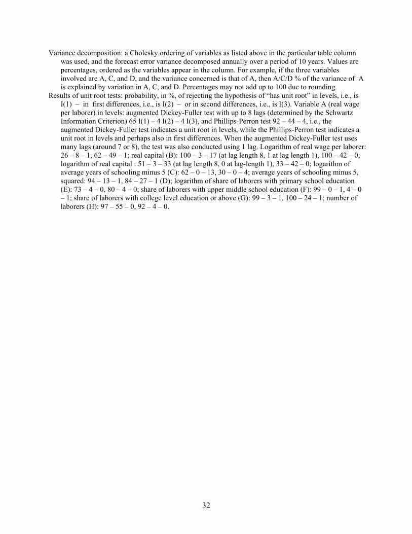
Variance decomposition: a Cholesky ordering of variables as listed above in the particular table column was used, and the forecast error variance decomposed annually over a period of 10 years. Values are percentages, ordered as the variables appear in the column. For example, if the three variables involved are A, C, and D, and the variance concerned is that of A, then A/C/D % of the variance of A is explained by variation in A, C, and D. Percentages may not add up to 100 due to rounding.

Results of unit root tests: probability, in %, of rejecting the hypothesis of “has unit root” in levels, i.e., is I(1) – in first differences, i.e., is I(2) – or in second differences, i.e., is I(3). Variable A (real wage per laborer) in levels: augmented Dickey-Fuller test with up to 8 lags (determined by the Schwartz Information Criterion) 65 I(1) – 4 I(2) – 4 I(3), and Phillips-Perron test 92 – 44 – 4, i.e., the augmented Dickey-Fuller test indicates a unit root in levels, while the Phillips-Perron test indicates a unit root in levels and perhaps also in first differences. When the augmented Dickey-Fuller test uses many lags (around 7 or 8), the test was also conducted using 1 lag. Logarithm of real wage per laborer: 26 – 8 – 1, 62 – 49 – 1; real capital (B): 100 – 3 – 17 (at lag length 8, 1 at lag length 1), 100 – 42 – 0; logarithm of real capital : 51 – 3 – 33 (at lag length 8, 0 at lag-length 1), 33 – 42 – 0; logarithm of average years of schooling minus 5 (C): 62 – 0 – 13, 30 – 0 – 4; average years of schooling minus 5, squared: 94 – 13 – 1, 84 – 27 – 1 (D); logarithm of share of laborers with primary school education (E): 73 – 4 – 0, 80 – 4 – 0; share of laborers with upper middle school education (F): 99 – 0 – 1, 4 – 0 – 1; share of laborers with college level education or above (G): 99 – 3 – 1, 100 – 24 – 1; number of laborers (H): 97 – 55 – 0, 92 – 4 – 0.

32

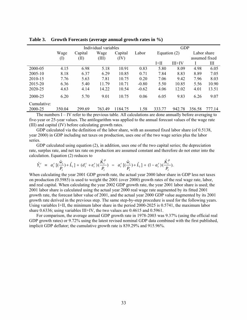
Table 3. Growth Forecasts (average annual growth rates in %)

Individual variables GDP Wage

(I) Capital

(II) Wage (III)

Capital (IV)

Labor Equation (2) Labor share assumed fixed

I+II III+IV I III 2000-05 4.15 6.98 5.18 10.91 0.83 5.80 8.09 4.98 6.052005-10 8.18 6.37 6.29 10.85 0.71 7.84 8.83 8.89 7.052010-15 7.76 5.63 7.81 10.75 0.20 7.06 9.42 7.96 8.032015-20 6.36 5.40 11.79 10.71 -0.80 5.50 10.85 5.56 10.902020-25 4.63 4.14 14.22 10.54 -0.62 4.06 12.02 4.01 13.51

2000-25 6.20 5.70 9.01 10.75 0.06 6.05 9.83 6.26 9.07

Cumulative: 2000-25 350.04 299.69 763.49 1184.75 1.58 333.77 942.78 356.58 777.14 The numbers I – IV refer to the previous table. All calculations are done annually before averaging to five-year or 25-year values. The antilogarithm was applied to the annual forecast values of the wage rate (III) and capital (IV) before calculating growth rates. GDP calculated via the definition of the labor share, with an assumed fixed labor share (of 0.5138, year 2000) in GDP including net taxes on production, uses one of the two wage series plus the labor series.

GDP calculated using equation (2), in addition, uses one of the two capital series; the depreciation rate, surplus rate, and net tax rate on production are assumed constant and therefore do not enter into the calculation. Equation (2) reduces to

).ˆ

()1(]ˆ)ˆ

[()ˆ

()(]ˆ)ˆ

[(ˆt

Pt

ttt

tt

t

Pt

tttt

ttt P

KaL

Pw

aP

KedL

Pw

aY ττττττ −++=+++≡

When calculating the year 2001 GDP growth rate, the actual year 2000 labor share in GDP less net taxes on production (0.5985) is used to weight the 2001 (over 2000) growth rates of the real wage rate, labor, and real capital. When calculating the year 2002 GDP growth rate, the year 2001 labor share is used; the 2001 labor share is calculated using the actual year 2000 real wage rate augmented by its fitted 2001 growth rate, the forecast labor value of 2001, and the actual year 2000 GDP value augmented by its 2001 growth rate derived in the previous step. The same step-by-step procedure is used for the following years. Using variables I+II, the minimum labor share in the period 2000-2025 is 0.5741, the maximum labor share 0.6336; using variables III+IV, the two values are 0.4615 and 0.5961. For comparison, the average annual GDP growth rate in 1978-2003 was 9.37% (using the official real GDP growth rates) or 9.72% using the latest revised nominal GDP data combined with the first published, implicit GDP deflator; the cumulative growth rate is 839.29% and 915.96%.

33

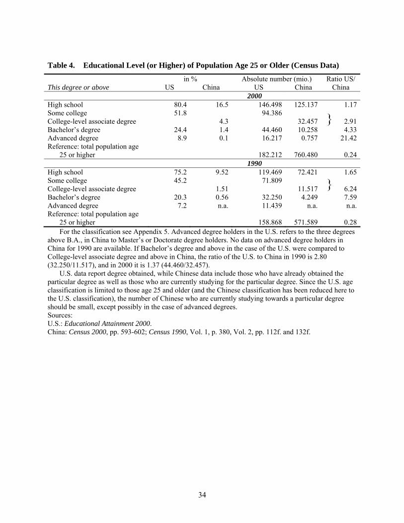
Table 4. Educational Level (or Higher) of Population Age 25 or Older (Census Data)

in % Absolute number (mio.) Ratio US/ This degree or above US China US China China 2000 High school 80.4 16.5 146.498 125.137 1.17Some college 51.8 94.386 College-level associate degree 4.3 32.457 2.91Bachelor’s degree 24.4 1.4 44.460 10.258 4.33Advanced degree 8.9 0.1 16.217 0.757 21.42Reference: total population age

25 or higher 182.212 760.480 0.24 1990 High school 75.2 9.52 119.469 72.421 1.65Some college 45.2 71.809 College-level associate degree 1.51 11.517 6.24Bachelor’s degree 20.3 0.56 32.250 4.249 7.59Advanced degree 7.2 n.a. 11.439 n.a. n.a.Reference: total population age

25 or higher 158.868 571.589 0.28

}

}

For the classification see Appendix 5. Advanced degree holders in the U.S. refers to the three degrees above B.A., in China to Master’s or Doctorate degree holders. No data on advanced degree holders in China for 1990 are available. If Bachelor’s degree and above in the case of the U.S. were compared to College-level associate degree and above in China, the ratio of the U.S. to China in 1990 is 2.80 (32.250/11.517), and in 2000 it is 1.37 (44.460/32.457).

U.S. data report degree obtained, while Chinese data include those who have already obtained the particular degree as well as those who are currently studying for the particular degree. Since the U.S. age classification is limited to those age 25 and older (and the Chinese classification has been reduced here to the U.S. classification), the number of Chinese who are currently studying towards a particular degree should be small, except possibly in the case of advanced degrees. Sources: U.S.: Educational Attainment 2000. China: Census 2000, pp. 593-602; Census 1990, Vol. 1, p. 380, Vol. 2, pp. 112f. and 132f.

34

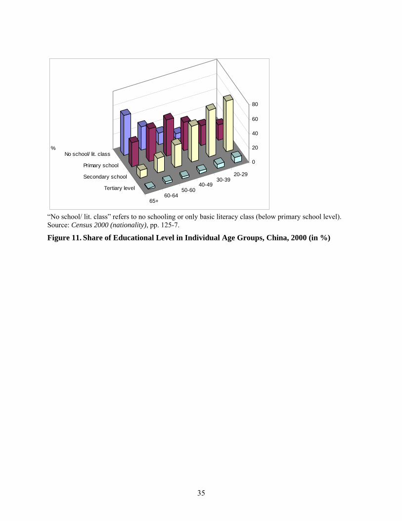
20-2930-39

40-4950-60

60-6465+

No school/ lit. class

Primary school

Secondary school

Tertiary level

0

20

40

60

80

%

“No school/ lit. class” refers to no schooling or only basic literacy class (below primary school level). Source: Census 2000 (nationality), pp. 125-7.

Figure 11. Share of Educational Level in Individual Age Groups, China, 2000 (in %)

35

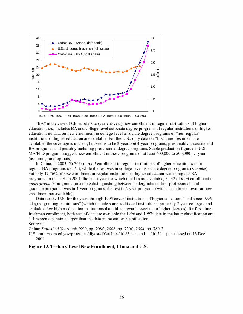
0

4

8

12

16

20

24

28

32

36

40

1978 1980 1982 1984 1986 1988 1990 1992 1994 1996 1998 2000 2002

100,

000

0.0

0.5

1.0

1.5

2.0

2.5

3.0

100,000

China: BA + Assoc. (left scale)

U.S.: Undergr. freshmen (left scale)

China: MA + PhD (right scale)

“BA” in the case of China refers to (current-year) new enrollment in regular institutions of higher education, i.e., includes BA and college-level associate degree programs of regular institutions of higher education; no data on new enrollment in college-level associate degree programs of “non-regular” institutions of higher education are available. For the U.S., only data on “first-time freshmen” are available; the coverage is unclear, but seems to be 2-year and 4-year programs, presumably associate and BA programs, and possibly including professional degree programs. Stable graduation figures in U.S. MA/PhD programs suggest new enrollment in these programs of at least 400,000 to 500,000 per year (assuming no drop-outs). In China, in 2003, 56.76% of total enrollment in regular institutions of higher education was in regular BA programs (benke), while the rest was in college-level associate degree programs (zhuanke); but only 47.76% of new enrollment in regular institutions of higher education was in regular BA programs. In the U.S. in 2001, the latest year for which the data are available, 54.42 of total enrollment in undergraduate programs (in a table distinguishing between undergraduate, first-professional, and graduate programs) was in 4-year programs, the rest in 2-year programs (with such a breakdown for new enrollment not available). Data for the U.S. for the years through 1995 cover “institutions of higher education,” and since 1996 “degree-granting institutions” (which include some additional institutions, primarily 2-year colleges, and exclude a few higher education institutions that did not award associate or higher degrees); for first-time freshmen enrollment, both sets of data are available for 1996 and 1997: data in the latter classification are 3-4 percentage points larger than the data in the earlier classification. Sources: China: Statistical Yearbook 1990, pp. 708f.; 2003, pp. 720f.; 2004, pp. 780-2. U.S.: http://nces.ed.gov/programs/digest/d03/tables/dt183.asp, and …/dt179.asp, accessed on 13 Dec.

2004.

Figure 12. Tertiary Level New Enrollment, China and U.S.

36

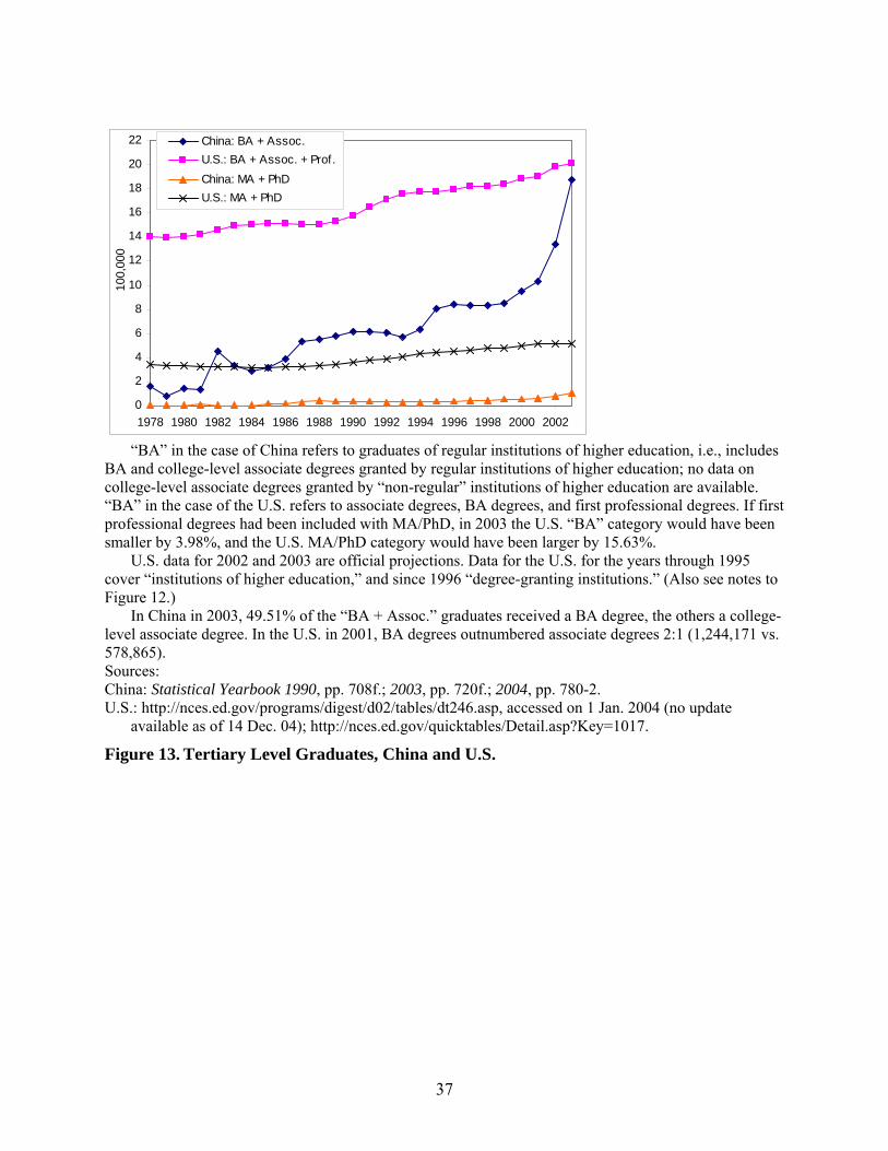
0

2

4

6

8

10

12

14

16

18

20

22

1978 1980 1982 1984 1986 1988 1990 1992 1994 1996 1998 2000 2002

100,

000

China: BA + Assoc.U.S.: BA + Assoc. + Prof.China: MA + PhDU.S.: MA + PhD

“BA” in the case of China refers to graduates of regular institutions of higher education, i.e., includes BA and college-level associate degrees granted by regular institutions of higher education; no data on college-level associate degrees granted by “non-regular” institutions of higher education are available. “BA” in the case of the U.S. refers to associate degrees, BA degrees, and first professional degrees. If first professional degrees had been included with MA/PhD, in 2003 the U.S. “BA” category would have been smaller by 3.98%, and the U.S. MA/PhD category would have been larger by 15.63%. U.S. data for 2002 and 2003 are official projections. Data for the U.S. for the years through 1995 cover “institutions of higher education,” and since 1996 “degree-granting institutions.” (Also see notes to Figure 12.) In China in 2003, 49.51% of the “BA + Assoc.” graduates received a BA degree, the others a college-level associate degree. In the U.S. in 2001, BA degrees outnumbered associate degrees 2:1 (1,244,171 vs. 578,865). Sources: China: Statistical Yearbook 1990, pp. 708f.; 2003, pp. 720f.; 2004, pp. 780-2. U.S.: http://nces.ed.gov/programs/digest/d02/tables/dt246.asp, accessed on 1 Jan. 2004 (no update

available as of 14 Dec. 04); http://nces.ed.gov/quicktables/Detail.asp?Key=1017.

Figure 13. Tertiary Level Graduates, China and U.S.

37

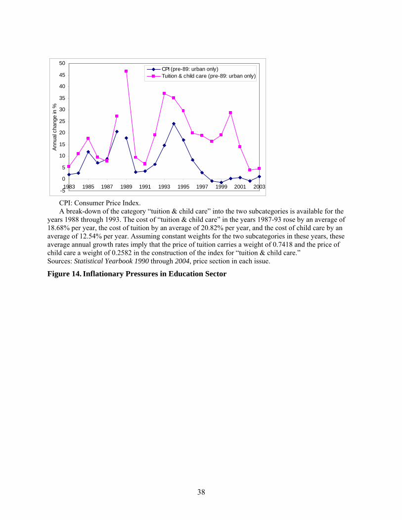
-5

0

5

10

15

20

25

30

35

40

45

50

1983 1985 1987 1989 1991 1993 1995 1997 1999 2001 2003

Annu

al c

hang

e in

%

CPI (pre-89: urban only)Tuition & child care (pre-89: urban only)

CPI: Consumer Price Index. A break-down of the category “tuition & child care” into the two subcategories is available for the years 1988 through 1993. The cost of “tuition & child care” in the years 1987-93 rose by an average of 18.68% per year, the cost of tuition by an average of 20.82% per year, and the cost of child care by an average of 12.54% per year. Assuming constant weights for the two subcategories in these years, these average annual growth rates imply that the price of tuition carries a weight of 0.7418 and the price of child care a weight of 0.2582 in the construction of the index for “tuition & child care.” Sources: Statistical Yearbook 1990 through 2004, price section in each issue.

Figure 14. Inflationary Pressures in Education Sector

38

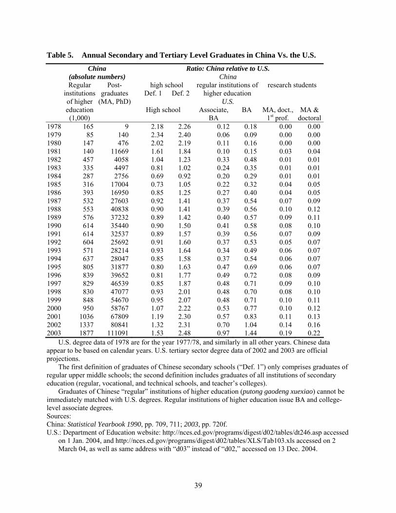
Table 5. Annual Secondary and Tertiary Level Graduates in China Vs. the U.S.

China Ratio: China relative to U.S. (absolute numbers) China Regular Post- high school regular institutions of research students institutions graduates Def. 1 Def. 2 higher education of higher (MA, PhD) U.S. education

(1,000) High school Associate,

BA BA MA, doct.,

1st prof. MA &

doctoral 1978 165 9 2.18 2.26 0.12 0.18 0.00 0.00 1979 85 140 2.34 2.40 0.06 0.09 0.00 0.00 1980 147 476 2.02 2.19 0.11 0.16 0.00 0.00 1981 140 11669 1.61 1.84 0.10 0.15 0.03 0.04 1982 457 4058 1.04 1.23 0.33 0.48 0.01 0.01 1983 335 4497 0.81 1.02 0.24 0.35 0.01 0.01 1984 287 2756 0.69 0.92 0.20 0.29 0.01 0.01 1985 316 17004 0.73 1.05 0.22 0.32 0.04 0.05 1986 393 16950 0.85 1.25 0.27 0.40 0.04 0.05 1987 532 27603 0.92 1.41 0.37 0.54 0.07 0.09 1988 553 40838 0.90 1.41 0.39 0.56 0.10 0.12 1989 576 37232 0.89 1.42 0.40 0.57 0.09 0.11 1990 614 35440 0.90 1.50 0.41 0.58 0.08 0.10 1991 614 32537 0.89 1.57 0.39 0.56 0.07 0.09 1992 604 25692 0.91 1.60 0.37 0.53 0.05 0.07 1993 571 28214 0.93 1.64 0.34 0.49 0.06 0.07 1994 637 28047 0.85 1.58 0.37 0.54 0.06 0.07 1995 805 31877 0.80 1.63 0.47 0.69 0.06 0.07 1996 839 39652 0.81 1.77 0.49 0.72 0.08 0.09 1997 829 46539 0.85 1.87 0.48 0.71 0.09 0.10 1998 830 47077 0.93 2.01 0.48 0.70 0.08 0.10 1999 848 54670 0.95 2.07 0.48 0.71 0.10 0.11 2000 950 58767 1.07 2.22 0.53 0.77 0.10 0.12 2001 1036 67809 1.19 2.30 0.57 0.83 0.11 0.13 2002 1337 80841 1.32 2.31 0.70 1.04 0.14 0.16 2003 1877 111091 1.53 2.48 0.97 1.44 0.19 0.22

U.S. degree data of 1978 are for the year 1977/78, and similarly in all other years. Chinese data appear to be based on calendar years. U.S. tertiary sector degree data of 2002 and 2003 are official projections.

The first definition of graduates of Chinese secondary schools (“Def. 1”) only comprises graduates of regular upper middle schools; the second definition includes graduates of all institutions of secondary education (regular, vocational, and technical schools, and teacher’s colleges).

Graduates of Chinese “regular” institutions of higher education (putong gaodeng xuexiao) cannot be immediately matched with U.S. degrees. Regular institutions of higher education issue BA and college-level associate degrees. Sources: China: Statistical Yearbook 1990, pp. 709, 711; 2003, pp. 720f. U.S.: Department of Education website: http://nces.ed.gov/programs/digest/d02/tables/dt246.asp accessed

on 1 Jan. 2004, and http://nces.ed.gov/programs/digest/d02/tables/XLS/Tab103.xls accessed on 2 March 04, as well as same address with “d03” instead of “d02,” accessed on 13 Dec. 2004.

39

Appendix 1. Data sources and explanations for Figure 1 through Figure 8

The wage rate is calculated as payments to labor (in the national income and product accounts) divided by economy-wide employment. Official employment data except for Taiwan are end-year data. When employment data are in the following related to annual flow measures, these end-year employment data are first turned into midyear values (the arithmetic mean of previous-year and current-year values); this is the case for sectoral labor productivity in China, the growth rate of real GDP per laborer, GDP per laborer, and wages per laborer. End-year values are used for the annual absolute change in the share of agriculture in employment, and for the share of agricultural laborers in economy-wide employment (Figure 3). Taiwan data are manipulated correspondingly. All data in Figure 6 are PWT data; population data are presumably end-year data and not further manipulated; country-specific investment prices (used in Figure 7, Figure 8) are also from the PWT. All online resources were accessed on or around 9 February 2004 unless otherwise noted. Japan Nominal and real GDP: World Bank Development Indicators database (at

http://www.worldbank.org/data/). Labor compensation in the income approach to GDP: Annual Report on National Income Statistics, various years, for 1953-89; http://portal.stat.go.jp/PubStat/topE.html for 1990-02.

Employment: Japan Statistical Yearbook 2004, p. 496. Employment data for agriculture, with corresponding total employment in the same table, are from the Annual Report on National Income Statistics, various years, for 1970-96, and from http://portal.stat.go.jp/PubStat/topE.html for 1997-2002. The total employment figures in these latter sources differ slightly from those in the Japan Statistical Yearbook 2004, and are only used for calculating the share of agricultural in employment.

Exchange rate: PWT (1960-1970), IFS (1971-2002). Korea All data are from the Korea National Statistical Office (at http://www.nso.go.kr). Taiwan Nominal and real GDP: Government statistics portal (at

http://www.stat.gov.tw/bs4/nis/enisd.htm) with online Statistical Yearbook (Taiwan) 2002. For labor compensation, in particular, Statistical Yearbook (Taiwan) 2002, p. 152; 2003, p. 152; and various earlier hardcopy issues.

Employment: online Statistical Yearbook (Taiwan) 2002, p. 48; 2003, pp. 43, 48; various earlier hardcopy issues; 2003 values (needed to derive end-year 2002 employment) from http://www.dgbas.gov.tw/public/data/dgbas03/bs7/yearbook/ch3/3-4.xls#a2, accessed on 20 May 05.

40

Exchange rate: online Statistical Yearbook (Taiwan) 2003, p. 246; IFS for years prior to 1973; PWT for 1951-1960. (In years for which separate buy and sell rates are given, the sell rate is used.)

China GDP: nominal GDP: Statistical Yearbook 2003, p. 55; real GDP growth: Statistical Yearbook

2003, p. 57; labor compensation: GDP 1952-95 (for 1978-92, 1995), various pages (sum across provinces); Statistical Yearbook, individual issues with data for 1993, 1994, and 1996-2002 (also sum across provinces); the share of sum-across-provinces labor compensation in sum-across-provinces income approach GDP is multiplied by the official (production approach) economy-wide GDP figure to obtain an estimate of economy-wide labor compensation.

Employment: aggregate: Statistical Yearbook 2003, p. 124; agriculture: Statistical Yearbook 1994, p. 86; 2003, p. 128. Between 1989 and 1990, China’s economy-wide number of laborers increased by 17.03%, with a 14.12% rise due to a post 1990-census switch to a new time series. Prior to 1990, the published economy-wide number of laborers constituted the sum of laborers across industrial sectors (hangye). Since 1990, the economy-wide number of laborers exceeds the sum across industrial sectors significantly in each year, but continues to, as in all reform years, equal the sum across economic sectors (chanye; primary, secondary, tertiary). Since the economy-wide number following the new time series for the years since 1990 is the one compiled according to international definitions of employment, the economy-wide number of laborers in the years prior to 1990 was adjusted following the population censuses of 1982 and 1990 (later-year official values rely on population census data). For details see Carsten Holz (2005b); the 1990 midyear census employment value is slightly above the 1990 end-year employment value in the Statistical Yearbook, which means that the mid-year 1991 employment value calculated from the Statistical Yearbook data is close to the 1990 midyear census employment value. No adjustment was attempted, and the 1991 growth rate in labor productivity is omitted from the charts . The share of agriculture (taken to be the primary sector) in economy-wide employment is in all years based on the official data; the statistical break 1989/90 occurs across all economic sectors and the total (employment in the three economic sectors always adds up to the total).

Exchange rate: IFS (for 1978-80); Statistical Yearbook 2001, p. 586 (for 1981-84); 2003, p. 654. Sectoral labor productivity growth rates (Figure 1) are based on 1978 aggregate value-added

(Statistical Yearbook 2004, p. 53) and cumulative real growth rates (same source, p. 56) combined with average annual employment derived from end-year labor data for the years 1977 through 2003 (Statistical Yearbook 2004, p. 120, for 1978 through 2003, and Fifty Years of New China, p. 2, for 1977); no adjustments for the statistical break in 1989/90 are made.

U.S. National income and product accounts data are from the BEA website at

http://www.bea.doc.gov/bea/dn1.htm. Employment data are from the BLS website at http://www.bls.gov/ (unadjusted employment

level, series LNU 02000000).

41

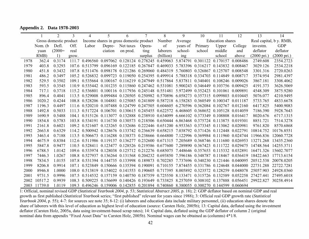
Appendix 2. Data 1978-2003

1 2 3 4 5 6 7 8 9 10 11 12 13 14 Gross domestic product Income shares in gross domestic product Number Average Education shares Real capital, b y. RMB,

Nom. (b yuan

RMB)

Defl. (2000=

1)

Off. real

grow.

Labor Depre-ciation

Net taxes on prod.

Opera-ting

surplus

of laborers (billion)

years of school-

ing

Primary school

Upper middle school

College and

above

investm. deflator

(2000 pri.)

GDP deflator

(2000 pri.) 1978 362.4 0.3174 111.7 0.496560 0.097062 0.128124 0.278245 0.459063 5.874791 0.301122 0.170157 0.008486 2749.608 2354.2723 1979 403.8 0.3293 107.6 0.513799 0.096169 0.122185 0.267847 0.469033 5.783396 0.316217 0.143832 0.008467 3029.126 2534.2218 1980 451.8 0.3432 107.8 0.511476 0.098178 0.121286 0.269060 0.484319 5.760803 0.326867 0.125707 0.008548 3301.316 2720.0263 1981 486.2 0.3497 105.2 0.526832 0.099723 0.119050 0.254395 0.499914 5.788318 0.334703 0.114849 0.008717 3574.954 2981.4397 1982 529.5 0.3502 109.1 0.535664 0.100167 0.116219 0.247949 0.517864 5.837811 0.340401 0.108246 0.009026 3867.181 3308.4062 1983 593.5 0.3545 110.9 0.535442 0.101235 0.115860 0.247462 0.531081 5.900243 0.346449 0.103756 0.009425 4191.373 3626.5069 1984 717.1 0.3718 115.2 0.536801 0.100116 0.117936 0.245148 0.551481 5.972499 0.352423 0.101061 0.009891 4548.309 3875.9280 1985 896.4 0.4041 113.5 0.529008 0.099484 0.120505 0.250982 0.570896 6.058273 0.357315 0.099803 0.010445 5076.077 4210.9495 1986 1020.2 0.4244 108.8 0.528206 0.104881 0.125085 0.241809 0.587218 6.158283 0.360549 0.100347 0.011187 5733.765 4833.6678 1987 1196.3 0.4497 111.6 0.520210 0.107488 0.124799 0.247505 0.604605 6.270596 0.362084 0.102767 0.012160 6417.825 5400.9083 1988 1492.8 0.5033 111.3 0.517224 0.106701 0.130615 0.245455 0.622572 6.468605 0.368652 0.105128 0.014059 7186.390 5928.7643 1989 1690.9 0.5488 104.1 0.515126 0.113077 0.132888 0.238910 0.634099 6.666102 0.373349 0.108808 0.016417 8020.676 6717.1315 1990 1854.8 0.5783 103.8 0.534191 0.116730 0.130573 0.218506 0.650444 6.863468 0.375724 0.113875 0.019301 8851.721 7514.3278 1991 2161.8 0.6021 109.2 0.521607 0.123265 0.132686 0.222446 0.651200 6.953363 0.373345 0.113062 0.020981 9761.820 8570.6868 1992 2663.8 0.6329 114.2 0.500942 0.128676 0.133742 0.236639 0.658215 7.038792 0.371426 0.112448 0.022791 10814.752 10176.8551 1993 3463.4 0.7188 113.5 0.506673 0.116288 0.138373 0.238666 0.664800 7.122996 0.369984 0.111960 0.024744 11966.836 12060.7728 1994 4675.9 0.8384 112.6 0.511986 0.119137 0.136277 0.232600 0.671315 7.205689 0.368746 0.111680 0.026953 13271.268 13435.2360 1995 5847.8 0.9477 110.5 0.528411 0.123477 0.128526 0.219586 0.677600 7.289890 0.367423 0.111722 0.029475 14748.564 14255.3711 1996 6788.5 1.0142 109.6 0.533974 0.128038 0.125712 0.212276 0.685075 7.448646 0.357653 0.115332 0.032891 16471.326 15602.7077 1997 7446.3 1.0267 108.8 0.527937 0.136264 0.131568 0.204232 0.693850 7.596186 0.348787 0.118467 0.036419 18422.663 17713.6154 1998 7834.5 1.0155 107.8 0.531394 0.144735 0.133998 0.189873 0.702285 7.737696 0.340230 0.121446 0.040095 20512.538 20078.0205 1999 8206.8 0.9914 107.1 0.523849 0.150666 0.135394 0.190091 0.710155 7.874455 0.331786 0.124648 0.044000 22731.288 22722.7281 2000 8946.8 1.0000 108.0 0.513819 0.154022 0.141553 0.190605 0.717395 8.005892 0.323572 0.128259 0.048078 25057.903 24928.0360 2001 9731.5 0.9996 107.5 0.514532 0.157159 0.140750 0.187559 0.725550 8.133471 0.315726 0.132589 0.052258 27427.441 27495.6018 2002 10517.2 0.9939 108.3 0.509225 0.156699 0.140426 0.193649 0.733825 8.257059 0.308102 0.137888 0.056451 29922.827 30258.4914 2003 11739.0 1.0119 109.3 0.496246 0.159006 0.142855 0.201894 0.740860 8.380055 0.300270 0.144599 0.060694

1: Official, nominal revised GDP (Statistical Yearbook 2004, p. 53; Statistical Abstract 2005, p. 18); 2: GDP deflator based on nominal GDP and real growth as first published (Statistical Yearbook series; “first published” relevant for years since 1988); 3: Official real GDP growth rate (Statistical Yearbook 2004, p. 55); 4-7: for sources see note 35; 8-12: (i) laborers and education data include military personnel, (ii) education shares denote the share of laborers with this level of education as highest level of education (source: Carsten Holz, 2005b); 13: Capital data, deflated using the investment deflator (Carsten Holz, 2005a, data using investment-based scrap rates); 14: Capital data, deflated using the GDP deflator of column 2 (original nominal data from appendix “Fixed Asset Data” to Carsten Holz, 2005b). Nominal wages can be obtained as (columns) 4*1/8.

42

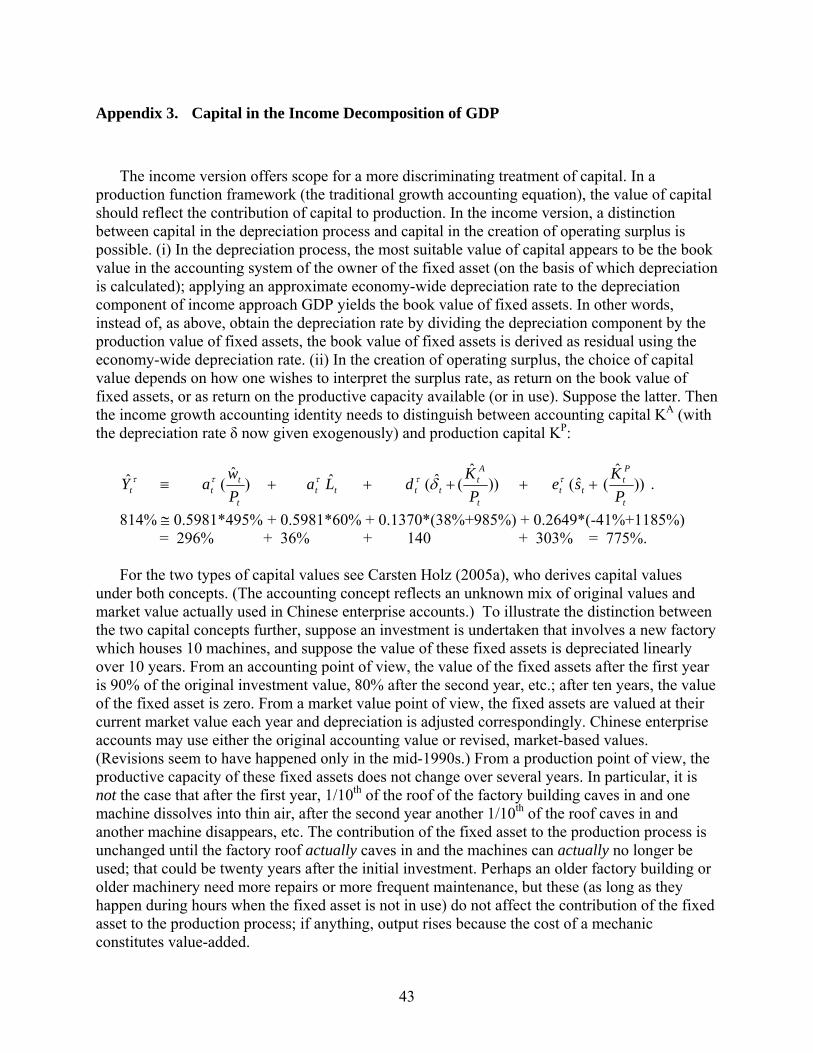
Appendix 3. Capital in the Income Decomposition of GDP

The income version offers scope for a more discriminating treatment of capital. In a production function framework (the traditional growth accounting equation), the value of capital should reflect the contribution of capital to production. In the income version, a distinction between capital in the depreciation process and capital in the creation of operating surplus is possible. (i) In the depreciation process, the most suitable value of capital appears to be the book value in the accounting system of the owner of the fixed asset (on the basis of which depreciation is calculated); applying an approximate economy-wide depreciation rate to the depreciation component of income approach GDP yields the book value of fixed assets. In other words, instead of, as above, obtain the depreciation rate by dividing the depreciation component by the production value of fixed assets, the book value of fixed assets is derived as residual using the economy-wide depreciation rate. (ii) In the creation of operating surplus, the choice of capital value depends on how one wishes to interpret the surplus rate, as return on the book value of fixed assets, or as return on the productive capacity available (or in use). Suppose the latter. Then the income growth accounting identity needs to distinguish between accounting capital KA (with the depreciation rate δ now given exogenously) and production capital KP:

))ˆ

(ˆ())ˆ

(ˆ(ˆ)ˆ

(ˆt

Pt

ttt

At

ttttt

ttt P

Kse

PK

dLaPw

aY +++++≡ τττττ δ .

814% ≅ 0.5981*495% + 0.5981*60% + 0.1370*(38%+985%) + 0.2649*(-41%+1185%) = 296% + 36% + 140 + 303% = 775%.

For the two types of capital values see Carsten Holz (2005a), who derives capital values under both concepts. (The accounting concept reflects an unknown mix of original values and market value actually used in Chinese enterprise accounts.) To illustrate the distinction between the two capital concepts further, suppose an investment is undertaken that involves a new factory which houses 10 machines, and suppose the value of these fixed assets is depreciated linearly over 10 years. From an accounting point of view, the value of the fixed assets after the first year is 90% of the original investment value, 80% after the second year, etc.; after ten years, the value of the fixed asset is zero. From a market value point of view, the fixed assets are valued at their current market value each year and depreciation is adjusted correspondingly. Chinese enterprise accounts may use either the original accounting value or revised, market-based values. (Revisions seem to have happened only in the mid-1990s.) From a production point of view, the productive capacity of these fixed assets does not change over several years. In particular, it is not the case that after the first year, 1/10th of the roof of the factory building caves in and one machine dissolves into thin air, after the second year another 1/10th of the roof caves in and another machine disappears, etc. The contribution of the fixed asset to the production process is unchanged until the factory roof actually caves in and the machines can actually no longer be used; that could be twenty years after the initial investment. Perhaps an older factory building or older machinery need more repairs or more frequent maintenance, but these (as long as they happen during hours when the fixed asset is not in use) do not affect the contribution of the fixed asset to the production process; if anything, output rises because the cost of a mechanic constitutes value-added.

43

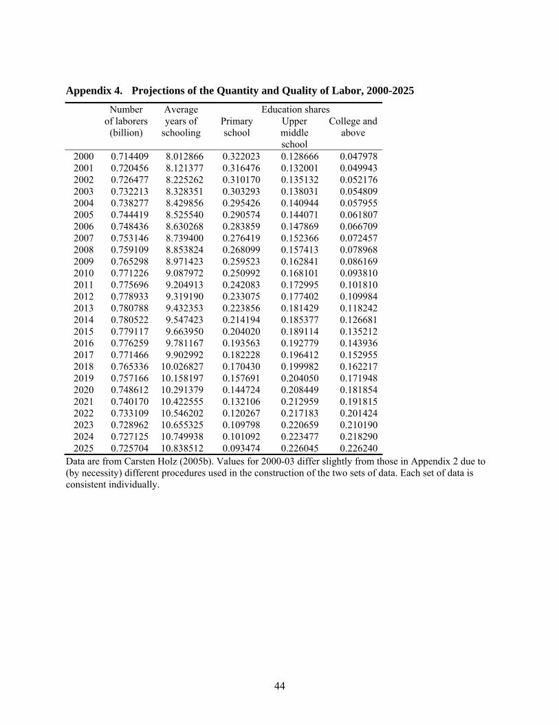
Appendix 4. Projections of the Quantity and Quality of Labor, 2000-2025

Number Average Education shares

of laborers (billion)

years of schooling

Primary school

Upper middle school

College and above

2000 0.714409 8.012866 0.322023 0.128666 0.0479782001 0.720456 8.121377 0.316476 0.132001 0.0499432002 0.726477 8.225262 0.310170 0.135132 0.0521762003 0.732213 8.328351 0.303293 0.138031 0.0548092004 0.738277 8.429856 0.295426 0.140944 0.0579552005 0.744419 8.525540 0.290574 0.144071 0.0618072006 0.748436 8.630268 0.283859 0.147869 0.0667092007 0.753146 8.739400 0.276419 0.152366 0.0724572008 0.759109 8.853824 0.268099 0.157413 0.0789682009 0.765298 8.971423 0.259523 0.162841 0.0861692010 0.771226 9.087972 0.250992 0.168101 0.0938102011 0.775696 9.204913 0.242083 0.172995 0.1018102012 0.778933 9.319190 0.233075 0.177402 0.1099842013 0.780788 9.432353 0.223856 0.181429 0.1182422014 0.780522 9.547423 0.214194 0.185377 0.1266812015 0.779117 9.663950 0.204020 0.189114 0.1352122016 0.776259 9.781167 0.193563 0.192779 0.1439362017 0.771466 9.902992 0.182228 0.196412 0.1529552018 0.765336 10.026827 0.170430 0.199982 0.1622172019 0.757166 10.158197 0.157691 0.204050 0.1719482020 0.748612 10.291379 0.144724 0.208449 0.1818542021 0.740170 10.422555 0.132106 0.212959 0.1918152022 0.733109 10.546202 0.120267 0.217183 0.2014242023 0.728962 10.655325 0.109798 0.220659 0.2101902024 0.727125 10.749938 0.101092 0.223477 0.2182902025 0.725704 10.838512 0.093474 0.226045 0.226240

Data are from Carsten Holz (2005b). Values for 2000-03 differ slightly from those in Appendix 2 due to (by necessity) different procedures used in the construction of the two sets of data. Each set of data is consistent individually.

44

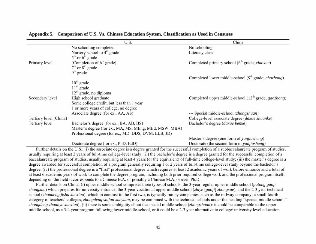
Appendix 5. Comparison of U.S. Vs. Chinese Education System, Classification as Used in Censuses

U.S. China No schooling completed No schooling Nursery school to 4th grade Literacy class 5th or 6th grade Primary level [Completion of 6th grade] Completed primary school (6th grade; xiaoxue) 7th or 8th grade

9

th grade Completed lower middle-school (9th grade; chuzhong) 10th grade 11th grade 12th grade, no diploma Secondary level High school graduate Completed upper middle-school (12th grade; gaozhong) Some college credit, but less than 1 year 1 or more years of college, no degree Associate degree (for ex., AA, AS) --- Special middle-school (zhongzhuan) Tertiary level (China) College-level associate degree (daxue zhuanke) Tertiary level Bachelor’s degree (for ex., BA, AB, BS) Bachelor’s degree (daxue benke) Master’s degree (for ex., MA, MS, MEng, MEd, MSW, MBA) Professional degree (for ex., MD, DDS, DVM, LLB, JD) Master’s degree (one form of yanjiusheng) Doctorate degree (for ex., PhD, EdD) Doctorate (the second form of yanjiusheng) Further details on the U.S.: (i) the associate degree is a degree granted for the successful completion of a subbaccalaureate program of studies, usually requiring at least 2 years of full-time college-level study; (ii) the bachelor’s degree is a degree granted for the successful completion of a baccalaureate program of studies, usually requiring at least 4 years (or the equivalent) of full-time college-level study; (iii) the master’s degree is a degree awarded for successful completion of a program generally requiring 1 or 2 years of full-time college-level study beyond the bachelor’s degree, (iv) the professional degree is a “first” professional degree which requires at least 2 academic years of work before entrance and a total of at least 6 academic years of work to complete the degree program, including both prior required college work and the professional program itself; depending on the field it corresponds to a Chinese B.A. or possibly a Chinese M.A. or even Ph.D. Further details on China: (i) upper middle-school comprises three types of schools, the 3-year regular upper middle school (putong gaoji zhongxue) which prepares for university entrance, the 3-year vocational upper middle school (zhiye [gaoji] zhongxue), and the 2-3 year technical school (zhondeng jishu xuexiao), which in contrast to the first two, is typically run by companies, such as the railway company; a small fourth category of teachers’ colleges, zhongdeng shifan xueyuan, may be combined with the technical schools under the heading “special middle school,” zhongdeng zhuanye xuexiao); (ii) there is some ambiguity about the special middle school (zhongzhuan): it could be comparable to the upper middle-school, as a 3-4 year program following lower middle-school, or it could be a 2-3 year alternative to college/ university level education

45

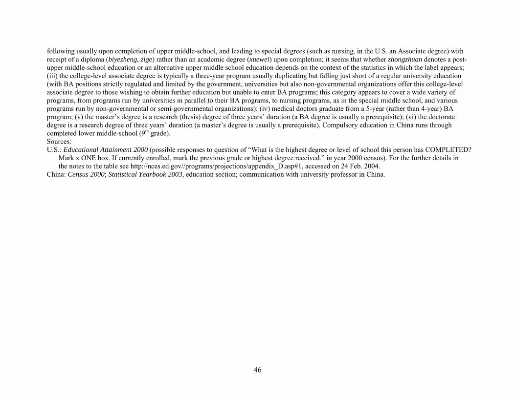
following usually upon completion of upper middle-school, and leading to special degrees (such as nursing, in the U.S. an Associate degree) with receipt of a diploma (biyezheng, zige) rather than an academic degree (xuewei) upon completion; it seems that whether zhongzhuan denotes a post-upper middle-school education or an alternative upper middle school education depends on the context of the statistics in which the label appears; (iii) the college-level associate degree is typically a three-year program usually duplicating but falling just short of a regular university education (with BA positions strictly regulated and limited by the government, universities but also non-governmental organizations offer this college-level associate degree to those wishing to obtain further education but unable to enter BA programs; this category appears to cover a wide variety of programs, from programs run by universities in parallel to their BA programs, to nursing programs, as in the special middle school, and various programs run by non-governmental or semi-governmental organizations); (iv) medical doctors graduate from a 5-year (rather than 4-year) BA program; (v) the master’s degree is a research (thesis) degree of three years’ duration (a BA degree is usually a prerequisite); (vi) the doctorate degree is a research degree of three years’ duration (a master’s degree is usually a prerequisite). Compulsory education in China runs through completed lower middle-school (9th grade). Sources: U.S.: Educational Attainment 2000 (possible responses to question of “What is the highest degree or level of school this person has COMPLETED?

Mark x ONE box. If currently enrolled, mark the previous grade or highest degree received.” in year 2000 census). For the further details in the notes to the table see http://nces.ed.gov//programs/projections/appendix_D.asp#1, accessed on 24 Feb. 2004.

China: Census 2000; Statistical Yearbook 2003, education section; communication with university professor in China.

46

Notes 1 Emma Broomfield (2003) provides an overview over the “China threat” literature. Stanley Lubman (2004) documents the negative views of China in U.S. congressional debates. 2 The quotes are from “The China Price” in Business Week, 6 Dec. 2004 (issue 3911), pp. 102ff. 3 China and France “compete” for fourth place, with the outcome depending on the exact Euro-USD exchange rate. (Statistical Abstract 2005, p. 203) 4 See The Economist, 15 Nov. 2003, p. 67, quoting the Bank Credit Analyst, a Canadian research firm. 5 This paper is also not concerned about how meaningful the concept of GDP data is for measuring “well-being” or “standard of living.” One may further question if value-added created in China contributes as much to well-being as does value-added created in the U.S., or vice-versa. Since the use of GDP as a measure of economic size, or, in per capita terms, as a proxy for standard of living, dominates in the literature as well as in popular discussions, this paper focuses on GDP. 6 See Statistical Yearbook 2003, p. 55; http://www.bea.doc.gov/bea/dn/gdplev.xls (accessed 19 May 2005). 7 See Statistical Communiqué 2004, p. 1; http://www.bea.doc.gov/bea/newsrelarchive/2005/gdp105a.xls (accessed 19 May 2005). Chinese GDP is 13.6515 trillion yuan RMB, the exchange rate 8.277 RMB per USD, and U.S. GDP 11.735 trillion USD. 8 Carsten Holz (2005c) argues that the manipulations, which follow a study by Angus Maddison, are not plausible. 9 A theoretical explanation for using real growth rates derived from nominal GDP and domestic prices rather than international prices is based on the Gerschenkron effect, namely that, empirically, the use of early-year prices leads to larger estimates of growth rates than the use of late-year prices (explained by the substitution effect from expensive to cheaper products); for developing countries, international prices are like “late-year” prices. Lawrence Klein and Suleyman Ozmucur (2003, p. 21f.), thus, feel that China’s purchasing power parity GDP growth rate is likely to be too low. On the other hand, Alan Heston, Daniel Nuxoll, and Robert Summers (1995) find just the reverse to be the case for the aggregate PWT data across the 116 countries in their study; they attribute their findings to the high level of aggregation in the PWT. 10 The PWT revised China’s official GDP value of 2000 (and earlier years) upward; this causes the cross-over year in the second scenario to be one year earlier than in the third scenario. 11 The price adjustment factor reflects three separate factors for investment, household consumption, and government consumption. The price adjustment factor in each of these three categories is a geometric mean of two values. (i) One value is an extrapolation from the 1985 PWT 5.6 value. This value in turn appears to incorporate a number of estimates by individual researchers. Ren Rouen and Chen Kai (1994) in a detailed study offer an adjustment factor for 1986 of approximately 3.8963. (I derived this numerical value by multiplying the average annual official exchange rate of 3.4543—the arithmetic mean of the four arithmetic means of beginning-quarter and end-quarter exchange rates in 1994—by Ren Rouen and Chen Kai’s convertor for RMB into USD of 1/0.8709. For the exchange rates see Financial Yearbook 1986, p. II-39; 1987, p. II-24.) (ii) The other value is a 1993 Guangdong vs. Hong Kong binary comparison value (downward adjusted in an attempt to reflect a multilateral basis). 12 The average annual per capita real growth rate of China’s richer coastal provinces used in the calculations here automatically incorporates the influx of people into the richer coastal provinces throughout the last two decades; i.e., by construction of the average, the newcomers to the rich areas have achieved the same average per capita GDP as the old inhabitants of the rich areas. There is no reason why this should not continue into the future (and the extrapolations here implicitly assume it does), leading to a larger share of China’s population (and thus a larger absolute number of Chinese people) enjoying the higher living standard in the future. If the official population data were to cover only the population registered with a regular residence right (hukou), the per capita GDP used in the coastal and six-province calculations here should be smaller; this is the case because, in current form, these per capita GDP data then do not incorporate laborers without regular residence in these provinces (which all experience labor inflows), but include the value-added they produce. This latter scenario is unlikely since the population data used are census data (see notes to ). The 2000 census of 1 November 2000 requires local presence for the past half year to be counted in a particular locality; the 1982 census of 1 July 1982 has a 1-year requirement but migrant labor was probably a phenomenon of negligible size in 1982.

Table 1

13 Reliable calculations based on employment are not possible. The PWT report per capita GDP in international dollars, as well as population data, but not employment data. The PWT also report per worker GDP in international dollars, with the underlying (but not reported) employment data purportedly from the International Labour Organization. For the case of China, combining the PWT data on “real GDP per capita (chain),” population, and “real GDP chain per worker” yields employment values that neither match the official data nor the author’s adjusted employment data (to bridge a statistical break in 1990). Compared to the author’s (through 1990) adjusted midyear

47

employment values, the PWT employment numbers are 13.00% larger in 1978 and 6.49% larger in 2000. The PWT population data, on the other hand, roughly match the official data published in the Statistical Yearbook. 14 In a different approach, Wing-Thye Woo (1999) examines the results of sector-level reforms in China, thus breaking the case of China down into several sectoral observations (which, however, are not independent). Thomas Rawski (1999) traces the interaction between different reforms; in total, these are taken to add up to the reform success. The World Bank (1997) examines a variety of “strengths and advantages” that it posits promote economic growth and a variety of “risks and challenges” that it thinks hamper economic growth” (p. 19). 15 Many constraints have disappeared after twenty-five years of reform. In terms of sales value, prices of approximately 90% of all goods have been liberalized. (See the Price Yearbook each year for the shares of prices that are market prices, mandatory prices, or guidance prices, for each of three categories: agricultural procurement, retail sales, and producer goods. It is questionable if “market prices” in China are truly market prices, and are so at all times.) State trading monopolies have largely disappeared. Export and import interventions (from administrative controls to quotas and tariffs/ subsidies) are all reaching the long-run levels committed to by China when joining the WTO. China has current account convertibility and partial capital account convertibility. Most sectors of China’s economy are open to new entry by enterprises in all ownership forms; in industry, for which detailed data are available, only 35% of value-added in 2003 was produced by state-owned or state-controlled enterprises. (Statistical Yearbook 2004, pp. 53, 518.) Other constraints remain, from ownership restrictions in the banking system to the appointment mechanisms in state-owned enterprises and the prohibition of land sales among farmers. 16 The first two are standard fare in development economics; see, for example, James Cypher and James Dietz (1997), pp. 27ff., 267, 403. The third is a basic theorem in trade theory as a corollary of the Heckscher-Ohlin theorem; see, for example, Dominick Salvatore (1998), Chapter 5. No attempt is made to control for the varying degrees to which these patterns might apply to a specific country at a given point of time (with variations in degree due to, for example, policy constraints). 17 Other East- or South-East Asian nations could have been included. The Philippines, in particular, would have been an interesting case due to the generally poor economic growth performance (significantly different values of the dependent variable than in the other four countries). But including the Philippines would have meant controlling for religion, and perhaps also for climate and ownership structure. This would imply gaining one degree of freedom (one extra observation, the Philippines), while at the same time losing between one and three degrees of freedom due to the new control variable(s), with no overall gain, if not a loss, of explanatory power. Singapore or Hong Kong would have required a city-state control variable, and perhaps a second control variable to account for the fact that Hong Kong since 1997 is part of China. Thailand and Malaysia would probably have confirmed the patterns observed for Korea and Taiwan. India may have needed a separate control variable for colonial history. Going further afield would have meant the necessity for more control variables, but the absence of data on one control variable even if in one country only would then have brought about the loss of this control variable, causing omitted variable bias. 18 Employment data for China experience a statistical break between 1989 and 1990 when total employment, following the 1990 population census, increases by 17.03%. In the following, total employment data for the years prior to 1990 are adjusted. For details see Carsten Holz (2005b). 19 This leaves unaddressed the question of how much catching up is feasible for a given country at a given time. Moses Abramovitz (1986) elaborates on the “social capability” to catch up and on the factors controlling the rate of realization of the potential for catching up (facilities for the diffusion of knowledge, conditions facilitating or hindering structural change, and macroeconomic and monetary conditions). 20 If the scope for catching up were measured by the labor productivity differences in the industrial sector only (rather than economy-wide), China’s highest level of catching up would probably be slightly higher, but not yet in the range where the corresponding growth rates of real GPD per laborer fall off significantly (see , Japan;

, Japan, Korea and Taiwan). Figure 4

4

Figure 621 These assumptions are: two countries; two commodities (goods); two factors of production; same, constant returns to scale technology in use in both countries; across both countries one commodity is labor intensive, the other capital intensive; incomplete specialization in production in both countries; tastes are equal in both countries; perfect competition in both goods and factor markets in both countries; perfect labor mobility within each country but no international factor mobility; no transportation costs, tariffs, or other obstructions to the free flow of international trade; all resources are fully employed in both countries; international trade between the two countries is balanced. (Dominick Salvatore, 1998, p. 110.) 22 The factor price equalization theorem would also appear to provide the basis of the “comparative-advantage following strategy” argued for by Justin Lin, Cai Fang, and Li Zhou (2003) 23 A chart with annual wages relative to the U.S., based on the absolute factor price equalization theorem, is very similar to Figure (with GDP per laborer as a measure of catching up) and omitted; this is due to the fact that labor

48

shares in GDP tend to be constant over time and similar across countries. (Wages are obtained by dividing the labor remuneration component of GPD by the number of laborers.) 24 Robert Barro and Xavier Sala-i-Martin (1995, p. 352) stress that “growth accounting does not … constitute a theory of economic growth because it does not attempt to explain how the changes in inputs and the improvements in total factor productivity relate to elements—such as aspects of preferences, technology, and government policies—that can reasonably be viewed as fundamentals.” However, what explains preferences, technology, and government policies? Trying to trace economic growth back to original causes presents a problem of infinite regress. The decision on when to stop, i.e., which level to view as ultimate “explanation,” appears arbitrary. 25 The growth rate is defined as percentage change. Using first differences of all variables in natural logarithms yields similar regression results. At China’s relatively large annual growth rates, the first differences of natural logarithms constitute an inexact approximation of the growth rates. For example, a 10% growth rate of, say, output, and a 15% growth rate of, say, capital, turn into 9.53% and 13.98% if natural logarithms are used. If growth rates are taken over several years, first differences of natural logarithms represent an increasingly inaccurate approximation of growth rates. 26 The results are sensitive to the particular capital measure used. The capital measure used in the reported results throughout this paper is the one identified as the most preferred one in Carsten Holz (2005a). With other capital series, the coefficient values change, but remain insignificant. 27 Gregory Chow Kui-Wai Li (2002) estimate the growth accounting equation (1) in logarithms for the years 1952-98, i.e., including the pre-reform period, but then excluding 1958-69. They correct for serial correlation. Their regression is also run imposing constant returns to scale. The coefficient estimates are significant and plausible in terms of factor shares. Imposing constant returns to scale on the reform period data here also yields significant and plausible results, which, however, disappear once serial correlation is corrected for. Gregory Chow and Kui-Wai Li ignore a statistical break in the labor series between 1989 and 1990. Their labor measure, in logs, jumps from 5.5329 to 6.3909; a note reports that adjustments for the statistical break do not change the results. Carsten Holz (2005b) addresses (adjusts for) the statistical break in the labor series and constructs economy-wide midyear labor values. Carsten Holz (2005a) raises a number of questions about the capital series used by Gregory Chow (1993) and Gregory Chow and Kui-Wai Li (2002). 28 If real GDP is obtained by applying the implicit deflator as first published to the official nominal GDP series, the labor coefficient in the first equation turns negative and halves in the second equation, but all coefficients remain insignificant. The rationale for using the implicit deflator as first published, i.e., as obtainable from nominal GDP data as first published combined with real GDP growth rates as first published, is the following. The National Bureau of Statistics in May 2005 provided final revised nominal GDP data for 2003, and similarly in previous years. When the NBS first published 2003 nominal GDP data in the Statistical Yearbook 2004 in fall 2004 (apart from earlier estimates), it is highly likely that it had available final price indices for all sectors. Most price indices are compiled monthly and published with little time lag. In sectors where base year prices are used, these apply only to the directly reporting enterprises, on which economic data are immediately available (and need no revisions later); the deflator for the whole sector is derived from the data reported by these enterprises on output in constant and fixed prices. In other words, the likelihood for a need to revise the implicit GDP deflator of 2003 after fall 2004 is near-zero. It is unclear why the NBS does (usually) not revise its published real growth rates; perhaps it is such a highly publicized and political figure that the originally published real growth rate becomes sacrosanct? 29 Alwyn Young (2003, p. 1232, note 17) reports that using the Tornqvist weighted sum of the sectoral real growth rates reduces the official GDP growth rate by 0.2% per year. His data are for 1978-98. He does not specify which sectoral breakdown he uses. I was unable to replicate his findings. Based on the real growth rates of the three economic sectors (primary, secondary, tertiary), using the Tornqvist method, average annual aggregate GDP real growth in the period 1978-98 was 0.05% below the official one (or 0.06% if the 1978 growth rate over 1977 is included); re-composing, in addition, secondary sector growth from that of industry and construction, and tertiary sector growth from that of all tertiary sector subsectors yields a 0.07% (0.09%) divergence. 30 Wang Yan and Yao Yudong (2003, p. 39) do not adopt Alwyn Young’s method because they feel that the surveys on which Alwyn Young bases his estimations are not representative samples. James Heckman (2005) argues that “the low private rate of return to education [of, depending on study, around 4% or 7%] does not reflect the true rate of return in the late 1980s or early 1990s. Labor markets were so distorted in China that wages did not reflect the true marginal contribution of educated labor to the economy.” James Heckman estimates a social return “as high as 30% or 40%” (p. 62). This severely questions, if not invalidates Alwyn Young’s weighting of education in the derivation of the growth rate of human capital, and subsequently questions the validity of Alwyn Young’s measures of the contribution of human capital to output growth. 31 Two other implications are no factor substitution between intermediate inputs and labor and capital, and an elasticity of substitution of unity. Switching to gross output value as the output variable and including intermediate

49

inputs on the right-hand side for the period 1978-2002 yields a highly significant coefficient of intermediate inputs but negative contributions to output growth (or output in logs) of labor and capital (both insignificant when growth accounting is in growth rates, and both significant when in logarithms). Switching to the translog production function (which makes no assumptions about the elasticity of substitution) leads to many significant coefficients but significant negative first-order effects of capital and coefficient values of labor and capital in the hundreds rather than in the expected factor share range. (In contrast, Wu Yanrui, 2004, estimates a frontier production function resembling a translog with restrictions, using a provincial-level panel data set for the years 1981-97, to obtain plausible coefficient estimates.) In both regressions, adding the average years of schooling of laborers does not change the results; education also comes with a negative coefficient (in the second regression it tends to be negative in all terms in which education appears). 32 The manipulations are: taking derivatives with respect to time, dividing by GDP, expanding right-hand side terms to be able to simplify some combinations of variables to factor shares, assuming factor shares and growth rates of the wage rate and of the rental rate of capital to be constant, integrating with respect to time, then taking antilogarithms. Also see Jesus Felipe and Carsten Holz (2001). The growth accounting equation as presented also follows from other production functions, such as the CES (if the elasticity of substitution approaches unity), the translog (if the additional terms are insignificant), or the general production function Yt = F(Kt, Lt, t). 33 See, for example, Ishaq Nadiri (1970, pp. 1145f.). In general, the assumption of an economy-wide aggregate production function requires stringent criteria. For example, with constant returns to scale, only two factors of production, and all technical change in form of capital-augmenting technical change, the necessary condition for aggregation is that all capital is perfectly substitutable. The basic farming utensils used by half of China’s laborers are unlikely to be suitable to etch transistors into microchips at China’s newest fabs. 34 See Jesus Felipe and Carsten Holz (2001) for the range of variation, determined in simulations, that yields “good” results of an estimated Cobb-Douglas production function (growth accounting equation). In the case of China in the period 1978 through 2002, the labor share is sufficiently stable with a standard deviation of only 0.0111, but the variations in the growth rates of wages and of the rental rate of capital are too high. 35 Provincial gross value-added in the income approach in most years, for most provinces, exactly equals provincial gross value-added in the production approach, China’s official approach to calculating GDP. But the sum of provincial gross value-added only closely, not perfectly matches China’s national GDP value; the NBS does not solely rely on the provincial data when deriving the national GDP value. In addition, a very few provinces do not report income components for some of the early reform years. As long as the discrepancy between sum provincial GDP and national GDP does not reflect a particular bias in the size of one or more of the different income components (and there is no reason why it should), the procedure used here yields accurate national income component values. The provincial data are from GDP 1952-95 for the years 1978-1995, and from GDP 1996-2002 for the years 1996-2002; since the mid-1990s, each issue of the annual Statistical Yearbook also reports the data of the previous year. 36 The definition of operating surplus in China follows the standard System of National Accounts promulgated by the United Nations. At the enterprise level, business profit equals profit net of investment returns and non-business revenues. Individual-owned enterprises with seven or fewer employees (getihu) by definition do not have any operating surplus; their operating surplus is subsumed in labor remuneration. In as far as the individual-owned economy grows over time relative to other ownership forms, operating surplus as a share of GDP is likely to fall. For details on the link between business profit (or profit) and the operating surplus see Carsten Holz (2003), pp. 88f. 37 Arnold Harberger (1998, p. 1) postulates a growth equation that attributes “to each factor a marginal product measured by its economic reward” in form of RKLwyp +Δ+ )(Δ = Δ + ρ δ , with the variables denoting initial general price level, change in output (GDP), initial real wage, change in labor input, initial real rate of return to capital, rate of real depreciation of capital, change in capital stock, and the residual interpreted as “real cost reduction.” Compared to the definitional identity of the income growth accounting equation (and incorporating the price level in the coefficients of capital rather than in capital), the real cost reduction in his postulated equation, once divided by output, is identical to the weighted growth rates of real wages, the real depreciation rate, the real rate of return, and a particular form of change in the rate of net taxes on production. 38 Since the right-hand side variables are deflated using the implicit GDP deflator as first published, real growth rates of GDP are also based on this deflator. GDP based on the official real growth rates (which are usually not revised, while nominal data are), grew by 759%. 39 The income version of the growth accounting equation allows a distinction between different capital concepts, such as an accounting vs. production concept, for the depreciation vs. the operating surplus component. The results are necessarily similar. Details are provided in Appendix 3.

50

40 Annual data on laborers by age and education for the period 1978-2003 are obtained / calculated from the 1982, 1990, and 2000 population censuses together with the 1987 and 1995 1% population sample surveys. Projections for the years 2000-2025 make use of year 2000 census data and past patterns and trends. All calculations and estimations are explained in Carsten Holz (2005b). 41 Alwyn Young (2003), for example, regresses individuals’ wages on gender, age (for which he has a total of 11 categories), and education (total of 4 categories). 42 The likelihood ratio statistics with a small-sample multiplication factor of T-c (T numbers of observations, c numbers of restrictions) as well as the Schwartz Information Criterion were used to determine when to stop reducing the number of lags. The number of observations was held constant across all lag lengths, but because the number of observations is so small (annual data for the years 1978-2002), alternatively, the values of the decision criteria were also calculated for the maximum number of observations at each lag length, and a multiplication factor of T was also used as an alternative with the likelihood ratio statistic. As a result of the different criteria, often more than one lag length appeared plausible. In that case, all relevant lag lengths were taken to the next step of cointegration testing. 43 The R2 values of the individual VEC equations all tend to be in the 0.8 and 0.9 range. Apart from the results reported in the table, many cointegration equations have insignificant coefficients, some cointegration equations have highly implausible coefficient values (and then always a comparatively poor fit when contrasted to the actual real wage rate series in a chart), and a very few, with significant and plausible coefficients, yield similar results as those reported in the table. The ones reported in the table have the best fit in a visual comparison of the actual and fitted values. 44 A different cointegration equation involving the share of laborers with primary school education rather than the share of laborers with upper middle school education exhibits strong Granger causality from both education variables to the wage series. The share of laborers with primary school education also has a negative coefficient. In a visual comparison of the actual wage series and these two fitted series, the fitted series reported in the table with the share of laborers with upper middle school education better matched the actual series. 45 Similarly, the largest share of the forecast error variance of the share of laborers with upper middle school education is due to its own shocks, but 60% of the forecast error variance of the share of laborers with college level education or above is explained by variation in the share of laborers with upper middle school education. The forecast error variance decomposition depends, in this particular instance, much on the Cholesky ordering of the variables. Reversing the order, 63% of the variance of the wage is explained by variation in the share of laborers at upper middle school. 46 Non-education variables are typically not cointegrated with the wage rate. Age, or age squared, does not have a unit root. The difference in the choice of variables for the cointegration equations in levels vs. in logarithms is necessitated by the fact that some variables have unit roots when the variable is measured in levels, but not when it is measured in logarithms, and vice-versa. For example, in levels, ‘average years of schooling minus five’ is not I(1) but I(2), while the share of laborers with college level education or above in logarithms is I(2). Average years of schooling is I(2) independent of if the variable is in levels or in logarithms. 47 The underlying predicted cumulative real growth rate of wages in the period 2000-03, for which actual values are available, is 10.11% and 16.52% compared to the actual cumulative real growth rate of 21.26%. 48 The labor share in GDP (not net of taxes) has been near-constant throughout the reform period, with a mean of 0.5210 and a standard deviation of 0.0111 in 1978-2002, i.e., the coefficient of variation is only 2%. 49 The U.S. and Chinese education systems are not perfectly comparable. Appendix 5 establishes the equivalence of different degrees in the two countries. Three main complications are the following. First, the Chinese special middle-school degree is at least equivalent to the U.S. high school degree, but possibly in some circumstances even to the U.S. post-high school associate degree. Second, while the U.S. and China have comparable BA degrees, the Chinese MA degree differs from the U.S. MA degree in that the Chinese MA degree is a three-year post-BA research (thesis) degree rather than a one- to two-year predominantly taught degree; the Chinese PhD differs from the U.S. PhD in that it requires a prior MA and in that it is usually obtained in three years’ time, compared to longer average study times for the U.S. PhD. Third, Chinese professional degrees are usually obtained in form of a BA, but may also take the form of an MA or PhD. 50 The educational level of the age cohorts in the late 40s may be exaggerated in that some upper middle school graduates in China during the Cultural Revolution may have enjoyed no more than a lower middle school education under the label of an upper middle school education. 51 The 2004 figure for China is from the Statistical Abstract 2005, p. 175, and the 2005 figure from Caijing, no. 134 (30 May 2005), p. 11. 52 This assumes a narrow definition of undergraduate level graduates in China and a broad definition for the case of the U.S. In the case of China, the data comprise college-level associate degrees and BA degrees of regular institutions of higher education, i.e., omit associate degrees issued by non-regular institutions of higher education. In

51

the case of the U.S., the data comprise associate degrees, BA degrees, and first professional degrees. In China, the number of (typically 3-year) college-level associate degrees and the number of BA degrees in 2003 were approximately equal. In the U.S., the second outnumber the first (in the U.S. 2-year programs) two to one. 53 The table also reports a ratio including, in the U.S. figure, recipients of first professional degrees. In this case, the ratio is slightly lower. But with Chinese medical doctors and lawyers primarily holding a BA degree (in the medical doctor’s case a 5-year BA program), it seems inappropriate to include graduates of medical and law schools in the U.S. case but not in the Chinese case. 54 These data ignore Chinese students studying abroad since no specific degree and program completion data are available on these. Assuming Chinese students abroad were all studying in MA and PhD programs abroad, their number in 2000 was equivalent to approximately one-third of year 2003 domestic MA and PhD graduates; the number of returning students after completed studies was one-sixth of the number of domestic MA and PhD graduates in 2003. 55 The low number of Chinese high school graduates in the early 1980s could coincide with the reduction in compulsory education from 12 to 9 years, the exact date of which I am not aware of (and which could vary across localities). 56 A breakdown of the “tuition and child care” price index into the two components tuition and child care is only available for 1988 through 1993. During these years, tuition prices rose almost twice as fast as child care prices; tuition had a three-quarter weight in the price index “tuition and child care.” For the data see the price section in the Price Yearbook 1989 through 1994. In 2001, the primary classification of the CPI into goods vs. services was replaced by eight categories, each of which contains sub-categories of goods and services. Thus, the former subcategory xueza baoyufei within the category services, in the source translated as “tuition and childcare,” was reclassified as a subcategory of “recreation, education, and culture;” in this process the Chinese but not the English title was rephrased (to become xueza tuoyoufei). The extremely fast rise in the price of tuition and child care is likely to still ignore the often extra fees paid in addition to the official tuition fees. 57 The head count comparison is furthermore likely to be incomplete, since education in China outside the regular institutions of higher education has not been taken into consideration, while the U.S. data make no distinction between “official” and “unofficial” education. For example, adult education outside the regular university system in China is not included in the tertiary education data presented. In 2001, 316,367 persons graduated with a degree from a tertiary level adult education institution. This number corresponds to just below 1‰ of the population age 25-40 on 1 November 2000. (Census 2000, Vol. 1, pp. 215-7; Education Yearbook 2002, p. 107) 58 There is little doubt that the Chinese education system is indeed capable of identifying the brightest children, with lower middle school to university admission now routinely based on entrance examinations. James Heckman (2005) expresses concern about financial hurdles for children from low-income families. 59 Given the demographics, why has China not “overtaken” the U.S. a long time ago? The immediate answer is China’s choice of economic system prior to 1978. With uniform wages and access to higher-level education severely limited, neither were incentives for human capital accumulation in place nor the opportunities available. For example, tertiary level education almost ceased during the Cultural Revolution. In 1971, a since 1949 low of 600 students are reported to have graduated from a regular institution of higher education, down from 186,000 in 1965; only by 1977 did the figure again reach the 1965 level, with 194,000 graduates. (Statistical Yearbook 1990, p. 709.) This means that among the older generations, only the generation born in or before the 1940s had some access to tertiary level education. 60 See Statistical Yearbook 2001, p. 80 (Balance of Payments), 2003, p. 67 (GDP), p. 654 (exchange rate). In France it was 28.54%, in Germany 33.76%, in the UK 27.90%, and in the relatively small South Korea 44.79%. (Data for all countries except China are from the IFS. The value of China’s exports of goods and services is not reported in the IFS, only the net export value, i.e., the difference of exports and imports of goods and services. The data on net exports and GDP for China in the IFS are virtually identical to those reported in China’s national income accounts in the Statistical Yearbook series.) 61 See Statistical Yearbook 2004, pp. 53, 84, 714. 62 These data do not include foreign-funded (or Hong Kong, Macau, Taiwan) stock companies in China. For the data see Statistical Yearbook 2004, p. 519. The industrial enterprises with annual sales revenue in excess of 5m yuan RMB in 2003 accounted for 79.09% of all industrial value-added in China (p. 53); some of the smaller enterprises could also be foreign-funded. 63 Qi Yuanjun (2005) presents an overview of progress towards the calculation of green GDP for China. No economy-wide figure appears as yet available, but work by the NBS and China’s National Environmental Protection Office has begun to put a framework for green GDP into place within 3-6 years.

52