economic development and industrial pollution in...

Topics in Middle Eastern and African Economies

Vol. 16, No. 1, May 2014

65

Economic Development and Industrial Pollution in the

Mediterranean Region: A Panel Data Analysis

Sevil Acar and Mahmut Tekce

S. Acar (Corresponding Author): Assistant Professor, Istanbul Kemerburgaz University,

Department of Economics, Bagcilar 34217 Istanbul, Turkey [email protected]

Phone: +90 212 604 0100 / 4064

M. Tekce: Associate Professor, Marmara University, Department of Economics, Goztepe

34722 Istanbul, Turkey [email protected]

Abstract: This paper aims to analyse the determinants of industrial pollution in selected

Mediterranean countries. As carbon dioxide (CO2) emerges as the main pollutant in the

industrial sector, per capita CO2 emissions from manufacturing industries and construction has

been taken as a proxy for industrial pollution. The study uses data from the World

Development Indicators for the period 1971-2010. The results from the panel data model

estimations indicate the existence of an inverse U-shaped relation between GDP per capita

and industrial pollution in selected Mediterranean countries, which validates the

Environmental Kuznets Curve hypothesis. In addition, the share of industry, per capita energy

use, population density and urbanization are found as significant determinants of industrial

emissions in the selected countries.

JEL Classification: O13, Q50, Q53

Keywords: economic growth; Environmental Kuznets Curve; industrial pollution;

Mediterranean region; panel data analysis

mailto:[email protected]

mailto:[email protected]


Vol. 16, No. 1, May 2014

66

1. Introduction

Over the last several decades, economic growth and the rapid increase in population have

raised concerns about the environmental sustainability of current economic systems, and these

concerns led to an increase in attention to the determinants of pollution stemming from the

main sectors of an economy. Accordingly, various scholars have analyzed the relationship

between environmental degradation and economic activity, usually shown by per capita

income, and tested the validity of the Environmental Kuznets Curve hypothesis, which is

illustrated by an inverse U-shaped relation between pollution and economic development. In

general, the use of biochemical oxygen demand as a measure of water pollution and carbon

dioxide (CO2) and sulphur dioxide (SO2) emissions as measures of air pollution have been

widely investigated to proxy environmental degradation.

As the concerns and questions about environmental sustainability grow louder, understanding

the determinants of pollution becomes increasingly important, as such detection would make

it easier to design and implement appropriate policies against pollution and environmental

degradation. Industry, as a highly energy-intensive sector, emerges as a sector that is

significantly responsible for carbon emissions, where industry is responsible for more than 30

percent of energy use and 20 percent of total carbon emissions. According to a report by the

Blacksmith Institute (2012), the health impact of industrial pollutants is almost equal to or

higher than some of the worst global diseases, including malaria and tuberculosis. Industrial

pollution depends on several factors, including production technology, quality of inputs, lack

of purification equipments, weak environmental regulations and lack of social concern for

environmental protection. In this context, determining the responsible factors of carbon

emissions in the industrial sector becomes a crucial topic.


Vol. 16, No. 1, May 2014

67

This paper aims to analyse the determinants of carbon emissions stemming from the industrial

sectors in selected Mediterranean countries. Section 2 overviews the relevant literature

regarding the economic growth-environmental pressure relationship, having a glance at

Environmental Kuznets Curve studies. Section 3 explains why a focus on carbon emissions in

the industrial sector is important and why the Mediterranean region is worth examining in that

context. Section 4 explains the structure and the results of the model explaining the

determinants of industrial pollution in the selected countries. Finally, Section 5 concludes.

2. Economic Development and Pollution: A Brief Literature Survey

The relation between economic development and environment and the biophysical constraints

to economic growth have been a topic of interest in the literature since the publication of The

Limits to Growth commissioned by the Club of Rome (Meadows et al., 1972). Since then, the

accelerating pace of environmental degradation and the alerting effects of climate change

enriched the literature on the determinants of pollution and the possible ways to cope with

those problems.

The most accredited approach for explaining the linkage of environment and economic

development has been the Environmental Kuznets Curve (EKC) hypothesis, which presumes

an inverted U-shaped relationship between selected pollution indicators and per capita

income, following the original Kuznets Curve approach that postulates a similar relationship

between income inequality and per capita income (Kuznets and Simon, 1955). In other

words, the EKC hypothesis assumes that as an economy experiences growth in terms of per

capita income, the emission level grows in the initial stages, reaches a peak level and then

starts declining after a threshold level of per capita income has been reached.


Vol. 16, No. 1, May 2014

68

Grossman and Krueger (1991) is cited as the first study to examine this relationship and

numerous theoretical and empirical studies followed them in investigating the linkage

between economic development and various indicators of pollution. Shafik and

Bandyopadhyay (1992), Panayotou (1993), Shafik (1994), Selden and Song (1995), Grossman

and Krueger (1995) and McConnell (1997) found empirical evidence in favour of the EKC.

However, there are also various studies, like Holtz-Eakin and Selden (1995), Cole et al.

(1997) and Stern (2004) that reject the existence of the EKC hypothesis and propose different

relationships between environmental damage and per capita income. For example, Stern

(1998) argues that the evidence on the inverted-U relationship is only valid for a limited

subset of environmental measures and that other pollution problems increase through the

existing income range.

When the factors that are responsible for shaping the relationship between economic growth

and environmental quality are examined, the literature shows that it is possible to aggregate

various factors under five headings (see Dinda, 2004).

The first one is income elasticity of environmental quality demand; when spending on clean

environment is assumed as a luxury good that has high income elasticity, the demand for

environmental amenities increases as the welfare of consumers rises.

The second factor is scale, technological and composition effects; following Grossman and

Krueger (1991), although economic growth leads to environmental degradation through a

scale effect in the initial stages and the change in the composition of the economy from

agriculture to industry, technological effect through the use and replacement of new and

cleaner technology and another composition effect from industry to services and knowledge-

based sectors are expected to improve environmental quality (Vukina et al., 1999).


Vol. 16, No. 1, May 2014

69

The effect of the liberalisation of international trade and investment flows is referred to as

another factor that links economic growth and environmental damage. On one hand, free trade

can be beneficial for the environment by raising the wealth of people in developing countries

and leading them to demand a cleaner environment (Antweiler et al., 2001); but on the other

hand, it is also capable of creating ‘pollution havens’ as production of certain goods and

foreign direct investment shift to countries that have low production costs due to low

environmental standards, which would create a ‘race to the bottom’ (Wheeler, 2000).

However, according to Dasgupta et al. (2002), in time, multinational companies respond to

investor and consumer pressure in their home countries and tend to raise environmental

standards in the countries in which they invest.

Another factor that is argued to create a linkage between economic growth and environmental

quality is the self-regulatory market mechanism. Market mechanism is expected to form that

relationship through several channels; for instance through the rise in the prices of natural

resources as their stocks decrease, where higher prices of natural resources would lead to a

shift toward less resource-intensive technologies (Torras and Boyce, 1998). However,

according to Hettige et al. (2000), higher energy prices also induce shifts from capital- and

energy-intensive production methods to more labour- and material-intensive techniques and

these shifts are expected to lead to more pollution.

Finally, the effect of regulations is analysed as a factor shaping the EKC, where it is argued

that economic growth leads to the advance of social institutions and environmental

regulations (Dasgupta et al., 2001) and also strengthens private property rights. According to

Cropper and Griffiths (1994), proper allocation of property rights leads to efficient resource

allocation, which helps to increase income and decrease environmental problems. For

example, Hettige et al. (2000) argue that the main factor behind the improvement in water

quality with increases in per capita income is stricter environmental regulation.


Vol. 16, No. 1, May 2014

70

In short, recent work has shown that an inverted-U shaped relationship between economic

development and pollution can be derived using a variety of modelling techniques and

assumptions, where structural change, technological advances and more effective regulation

can also be regarded as potentially important sources of change in pollution (Hettige et al.,

2000).

3. Trends in Industrial CO2 Emissions in the Mediterranean Region

3.1. Industry and pollution

Industry is a highly energy-intensive sector constituting nearly one-third of global energy

demand, and 20 percent of worldwide CO2 emissions are attributable to industrial activities

(IEA, 2012) as shown in Figure 1. Both energy demand and carbon emissions from industry

are expected to rise in the forthcoming decades. ExxonMobil (2013) expects the industrial

demand for energy, including electricity, to grow by about 30 percent from 2010 to 2040,

where about 90 percent of the increase in industrial energy demand will come from

manufacturing and chemicals. This is expected to lead to significant increases in the

emissions from this sector. According to IEA (2010), without widespread deployment of

carbon capture and storage technologies, total direct and indirect emissions from industry are

expected to rise between 2007 and 2050 by 74% to 91%. As shown in Figure 2, carbon

emissions from industry are dominated by the production of goods in iron and steel, cement

and chemicals and petrochemicals.


Vol. 16, No. 1, May 2014

71

Figure 1: World CO2 emissions by sector (2010)

Source: IEA (2012, p. 9)

Figure 2: Total direct CO2 emissions from industry (2007)

Source: Brown et al. (2012, p. 4)

Fossil fuels currently constitute 70% of the total final energy used in industry and as Brown et

al. (2012) stress, the options for replacing fossil fuels or switching to less carbon intensive

fossil fuels are limited by currently available technologies. According to the forecasts of the

Residential 6%

Other 10%

Electricity and heat 42%

Transport 22%

Industry 20%

0%

Chemicals and petrochemicals

17% Pulp and paper

2%

Aluminium 2%

Iron and Steel 30% Cement

26%

Other 23%


Vol. 16, No. 1, May 2014

72

IEA (2010), fossil fuels are expected to remain the predominant source of energy in industry

even in the year 2050.

3.2. Industrial pollution in the Mediterranean region

The focus of this paper is on industrial pollution in the Mediterranean region and it aims to

capture the determinants of industrial pollution in selected countries of the Mediterranean

region.1

Evidently, the countries examined are heterogeneous in development level, size and

population, but the common feature is that, although the share of industry value added in their

GDP falls throughout the years, the size of the industrial sector in terms of value added in

constant USD is still high and in most cases has been on a constant rise after the 1980s,

especially in the developing countries of the region.

Similarly to all parts of the world with a high level of economic activity and large population,

industrial pollution has become increasingly alarming in the Mediterranean region. The

environment of the region is one of the richest in terms of biodiversity, but also one of the

most vulnerable in the world in the sense that the Mediterranean Sea and its coasts are the

source for many of the resources harvested in the region, an important hub for global trade,

and also the sink for the negative environmental impacts of these economic activities. These

characteristics, combined with the political complexity of the region, imply that the

management and protection of the coastal and marine environment will require multilateral

environmental agreements and regulations, abided by at a supranational level (UNEP/MAP,

2012).

1 Albania, Algeria, Cyprus, Egypt, France, Greece, Italy, Lebanon, Malta, Morocco, Spain, Syria, Tunisia and

Turkey.


Vol. 16, No. 1, May 2014

73

Environmental degradation in the Mediterranean region has been placed in the political

agenda since the mid-1970s, where the Barcelona Convention for the Protection of the

Mediterranean Sea against Pollution was amended in 1976. This Convention was extended to

include coastal areas in 1995 and in the same year a Mediterranean Commission on

Sustainable Development was created. As a part of the European Neighbourhood Policy, the

European Commission published a Commission Communication establishing an

environmental strategy for the Mediterranean and outlined the aims of the strategy as;

reducing pollution levels across the region, promoting sustainable use of the sea and its

coastline, encouraging neighbouring countries to cooperate on environmental issues, assisting

partner countries in developing effective institutions and policies to protect the environment,

and involving NGOs and the public in environmental decisions affecting them (European

Commission, 2006).

Future trends in Mediterranean coastal areas raise questions and concerns. Transport, tourism

and industrial infrastructures are concentrated on the coastal areas of the region, and it is

expected that by 2025 coastal urban populations will increase by 20 million, tourist flows will

double, and nearly 50 percent of the coastline will be built-up versus 40 percent in 2000

(Benoit and Comeau, 2006). Excessive coastal population and urbanization, combined with

increasing demand for industrial production, make the region vulnerable to environmental and

social risks.

When the selected countries of the Mediterranean region are analyzed, it is observed that,

except for two countries (Albania and Tunisia), the share of carbon emissions from

manufacturing industries and construction in total carbon emissions is below the global level.


Vol. 16, No. 1, May 2014

74

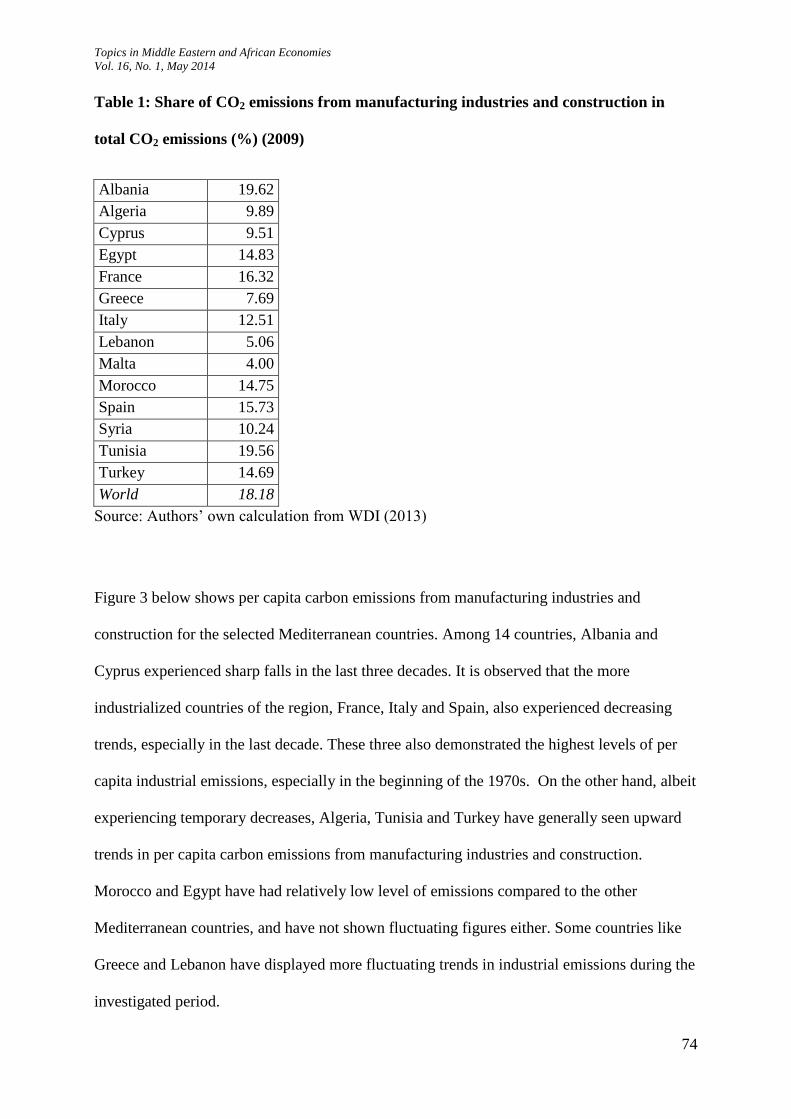
Table 1: Share of CO2 emissions from manufacturing industries and construction in

total CO2 emissions (%) (2009)

Albania 19.62

Algeria 9.89

Cyprus 9.51

Egypt 14.83

France 16.32

Greece 7.69

Italy 12.51

Lebanon 5.06

Malta 4.00

Morocco 14.75

Spain 15.73

Syria 10.24

Tunisia 19.56

Turkey 14.69

World 18.18

Source: Authors’ own calculation from WDI (2013)

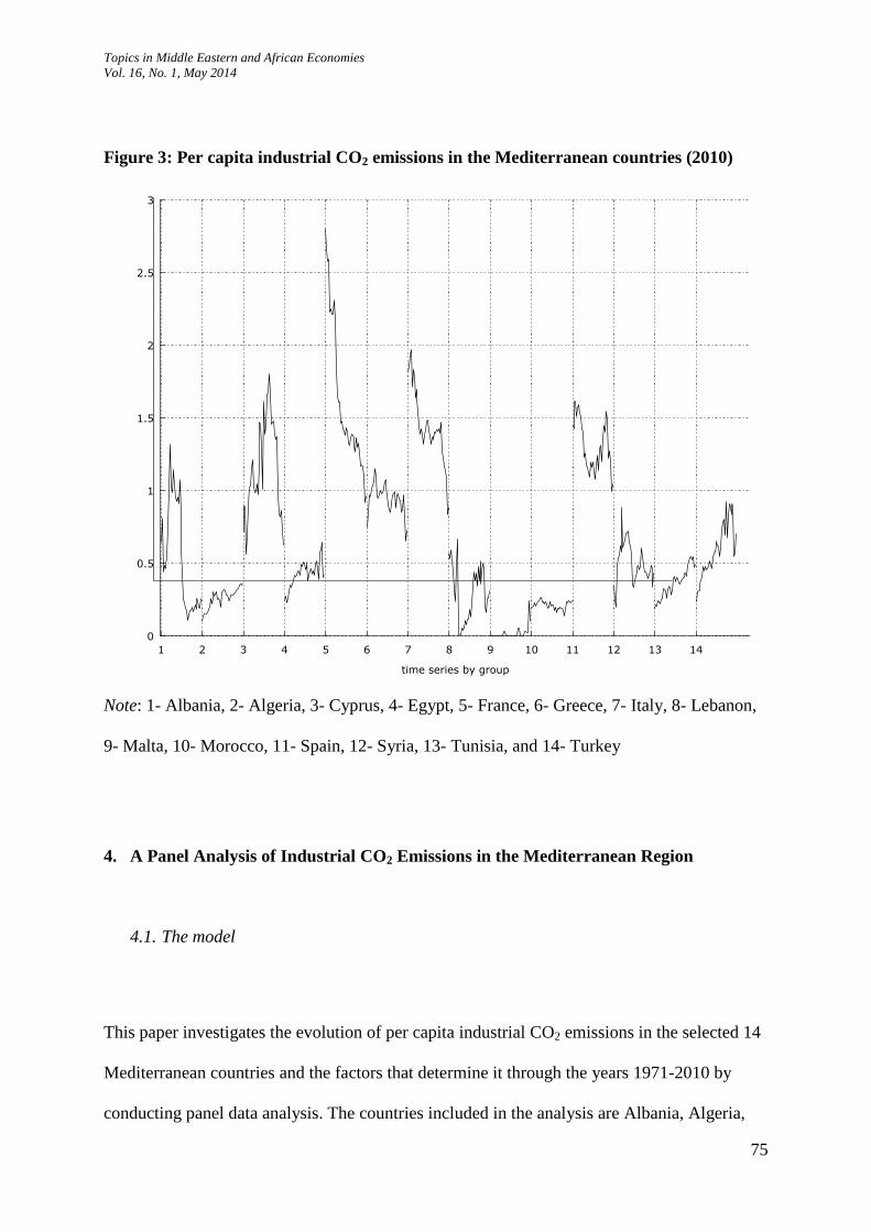
Figure 3 below shows per capita carbon emissions from manufacturing industries and

construction for the selected Mediterranean countries. Among 14 countries, Albania and

Cyprus experienced sharp falls in the last three decades. It is observed that the more

industrialized countries of the region, France, Italy and Spain, also experienced decreasing

trends, especially in the last decade. These three also demonstrated the highest levels of per

capita industrial emissions, especially in the beginning of the 1970s. On the other hand, albeit

experiencing temporary decreases, Algeria, Tunisia and Turkey have generally seen upward

trends in per capita carbon emissions from manufacturing industries and construction.

Morocco and Egypt have had relatively low level of emissions compared to the other

Mediterranean countries, and have not shown fluctuating figures either. Some countries like

Greece and Lebanon have displayed more fluctuating trends in industrial emissions during the

investigated period.


Vol. 16, No. 1, May 2014

75

Figure 3: Per capita industrial CO2 emissions in the Mediterranean countries (2010)

Note: 1- Albania, 2- Algeria, 3- Cyprus, 4- Egypt, 5- France, 6- Greece, 7- Italy, 8- Lebanon,

9- Malta, 10- Morocco, 11- Spain, 12- Syria, 13- Tunisia, and 14- Turkey

4. A Panel Analysis of Industrial CO2 Emissions in the Mediterranean Region

4.1. The model

This paper investigates the evolution of per capita industrial CO2 emissions in the selected 14

Mediterranean countries and the factors that determine it through the years 1971-2010 by

conducting panel data analysis. The countries included in the analysis are Albania, Algeria,

0

0.5

1

1.5

2

2.5

3

1 2 3 4 5 6 7 8 9 10 11 12 13 14

indCO

2pc

time series by group


Vol. 16, No. 1, May 2014

76

Cyprus, Egypt, France, Greece, Italy, Lebanon, Malta, Morocco, Spain, Syria, Tunisia and

Turkey. Other Mediterranean countries such as Israel and Libya had to be left out of the

analysis due to the lack of data for some necessary variables.

The analysis focuses on two issues; one is to explore whether an EKC relationship exists for

the countries of the region during the selected time period and the other is to search for the

possible determinants of per capita industrial CO2 emissions.

First, the EKC relationship is tested using the following standard specification:

Here the dependent variable is indCO2pc, i.e. per capita industrial CO2 emissions (in metric

tons), which are composed of CO2 emissions from manufacturing industries and construction

containing emissions from combustion of fuels in industry (extracted from WDI, 2013). On

the other hand, corresponds to lngdppc, which is taken as the natural logarithm of PPP-

converted GDP per capita at 2005 constant prices (extracted from Penn World Tables, 2012).

The existence of second and third exponents of income in the regression equation enables us

to test for various forms of environmental pressure - income relationships. For instance, if we

end up with = = , that means there is no relationship between environmental

pollution and income. On the other hand, the case where the coefficients appear to be such

that > 0, < 0 and coincides with an inverted-U shaped figure, namely the EKC

relationship. Other potential outcomes for coefficient estimates of income might result in N-

shaped, S-shaped or U-shaped figures as well as monotonic increasing or decreasing

relationships.


Vol. 16, No. 1, May 2014

77

In the second set of analyses, an array of economic indicators is added to income per capita

variables in order to offer an explanation for per capita industrial CO2 emissions. The model

is as follows:

where is composed of the following set of variables:

industry: Industry, value added (% of GDP)

urban: Urban population (% of total)

popdens: Population density (people per sq. km of land area)

trade: Trade (% of GDP)

energyuse: Energy use (kg of oil equivalent per capita)

All variables are taken from the World Development Indicators (World Bank, 2013) and used

in levels except lngdppc.2 Income per capita date from Penn World Tables is logged in order

to avoid extreme positive skewness.

Industry value added share of total output is used with the aim of revealing the economic

structure of domestic economies. According to the World Bank (2013) definitions, industry

corresponds to “ISIC divisions 10-45 and includes manufacturing (ISIC divisions 15-37). It

comprises value added in mining, manufacturing (also reported as a separate subgroup),

2 Summary statistics and correlation matrix for the variables are displayed in Appendices A and B.


Vol. 16, No. 1, May 2014

78

construction, electricity, water, and gas.” As such, we intend to account for all the polluting

and non-polluting industries of each economy in determining the impact on CO2 emissions.

Urban share of population is a potential factor for increasing industrial emissions. Again

according to the World Bank (2013), “urban population refers to people living in urban areas

as defined by national statistical offices. It is calculated using World Bank population

estimates and urban ratios from the United Nations World Urbanization Prospects.” As more

people live in urban areas either due to increased population or migration from rural to urban,

it is expected that more industrial activities will take place in the urban, possibly generating

more pollution. Another population measure that is utilised in this paper is population density,

which is defined as “the midyear population divided by land area in square kilometres”

(World Bank, 2013). Countries with higher population density are expected to suffer more

from industrial emissions owing to the fact that much denser economic activity takes place in

more populated areas.

Trade is another indicator that is expected to be influential on industrial emissions, since most

industrial production is feasible thanks to imports and exports of various goods. If industries

import polluting inputs (raw materials, intermediate goods, etc.) in order to employ during

their production processes, this has a direct or indirect impact on the amount of CO2

emissions. Besides, if industries are mainly export-oriented and produce polluting goods to

sell abroad, the consequences are again unfavourable for the domestic environment. Needless

to say, what matters is the structural composition as well as the production technology

(whether environmentally-friendly or not) of both imports and exports of a country.

Finally, varying levels of per capita energy use is expected to bear different outcomes in terms

of industrial emissions. It would be even more appropriate to examine what sources of energy

are utilized and which sectors use more energy. However, due to a lack of detailed statistics


Vol. 16, No. 1, May 2014

79

for the region, this study relies upon per capita energy use in general for each country. Energy

use is defined as “the use of primary energy before transformation to other end-use fuels,

which is equal to indigenous production plus imports and stock changes, minus exports and

fuels supplied to ships and aircraft engaged in international transport” by the World Bank

(2013) and is expected to cause higher emissions per capita in countries where primary energy

is excessively used. Different uses ranging from residential and commercial to transport and

industrial purposes are included under the same heading.

Panel fixed-effects estimations are employed for both model specifications. The reason why

fixed effects are preferred to another sort of estimation is that it allows for endogeneity of all

the regressors with these individual effects.3 On the contrary, for instance, when random

effects models are considered, all the regressors are assumed to be exogenous with random

individual effects, which, usually is not the case (Baltagi, 2005: 19). In our models, as well,

there is a potential of endogeneity among some variables, such as population density and

industrial emissions. We aim at looking at the effect of population on CO2 emissions, whereas

the causal link from emissions to population density is also a possible one. People might

prefer to live in places where industrial pollution is not a serious threat. Hence, we are content

with fixed effects estimations which permit such a possibility. Besides, all the models

consider time fixed effects and robust standard errors against heteroskedasticity. We choose

the “heteroskedasticity and autocorrelation consistent” (HAC) approach suggested by

Arellano (2003) to arrive at asymptotically valid estimates of the covariance matrix in the

case of both heteroskedasticity and autocorrelation of the error process.

3 The choice between the fixed- and random-effects estimators is further explored by Mundlak (1978).


Vol. 16, No. 1, May 2014

80

4.2. Empirical results

In Model 1 and 2, we test the EKC hypothesis via a third degree polynomial function of

income per capita (in natural logs), whereas in Model 3, we estimate a quadratic form

equation since the coefficients for the cubic form in Model 2 end up being insignificant.

Model 2 and 3 include the economic variables mentioned above in addition to income per

capita.

The findings in the first column of Table 2 reveal that per capita industrial CO2 emissions

initially decline with rising per capita income, then start to rise after a certain income level is

reached and finally decline again after a higher per capita income level. This finding does not

support the EKC hypothesis, which would imply an inverted-U curve and hence in a

cubic model specification. Instead, we are faced with a tilted-S curve with -, +, - signs for

coefficients respectively. But one implication of the Model 1 results is that

there is a point in time when industrial emissions start to decline when the Mediterranean

countries reach a certain income point.

Besides, although not all the time dummies are significant in Model 1, some years, such as

2008, 2009 and 2010, contribute significantly to the decline of industrial emissions (as

compared to the year 1971).4

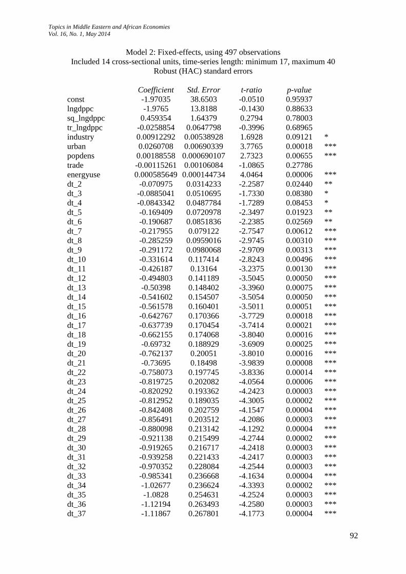
Model 2 incorporates the impact of different factors together with per capita income (and its

exponents) that might affect industrial CO2 emissions in the Mediterranean region (see the

second column in Table 2). This specification indicates the positive effects of industry,

urbanization, population density and energy use on industrial CO2 emissions. In other words,

higher shares of industry value-added in total output, urban population, population density

4Regression outputs are displayed in Appendix C.


Vol. 16, No. 1, May 2014

81

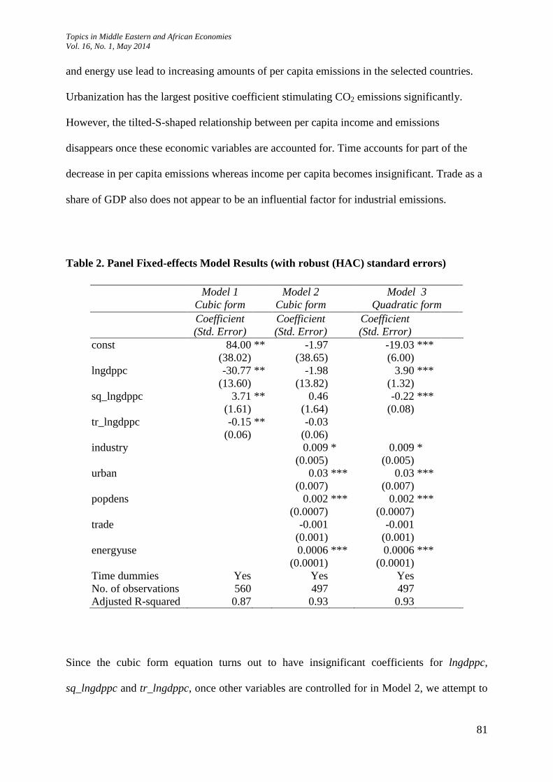
and energy use lead to increasing amounts of per capita emissions in the selected countries.

Urbanization has the largest positive coefficient stimulating CO2 emissions significantly.

However, the tilted-S-shaped relationship between per capita income and emissions

disappears once these economic variables are accounted for. Time accounts for part of the

decrease in per capita emissions whereas income per capita becomes insignificant. Trade as a

share of GDP also does not appear to be an influential factor for industrial emissions.

Table 2. Panel Fixed-effects Model Results (with robust (HAC) standard errors)

Model 1

Cubic form

Model 2

Cubic form

Model 3

Quadratic form

Coefficient

(Std. Error)

Coefficient

(Std. Error)

Coefficient

(Std. Error)

const 84.00 ** -1.97 -19.03 ***

(38.02) (38.65) (6.00)

lngdppc -30.77 ** -1.98 3.90 ***

(13.60) (13.82) (1.32)

sq_lngdppc 3.71 ** 0.46 -0.22 ***

(1.61) (1.64) (0.08)

tr_lngdppc -0.15 ** -0.03

(0.06) (0.06)

industry 0.009 * 0.009 *

(0.005) (0.005)

urban 0.03 *** 0.03 ***

(0.007) (0.007)

popdens 0.002 *** 0.002 ***

(0.0007) (0.0007)

trade -0.001 -0.001

(0.001) (0.001)

energyuse 0.0006 *** 0.0006 ***

(0.0001) (0.0001)

Time dummies Yes Yes Yes

No. of observations 560 497 497

Adjusted R-squared 0.87 0.93 0.93

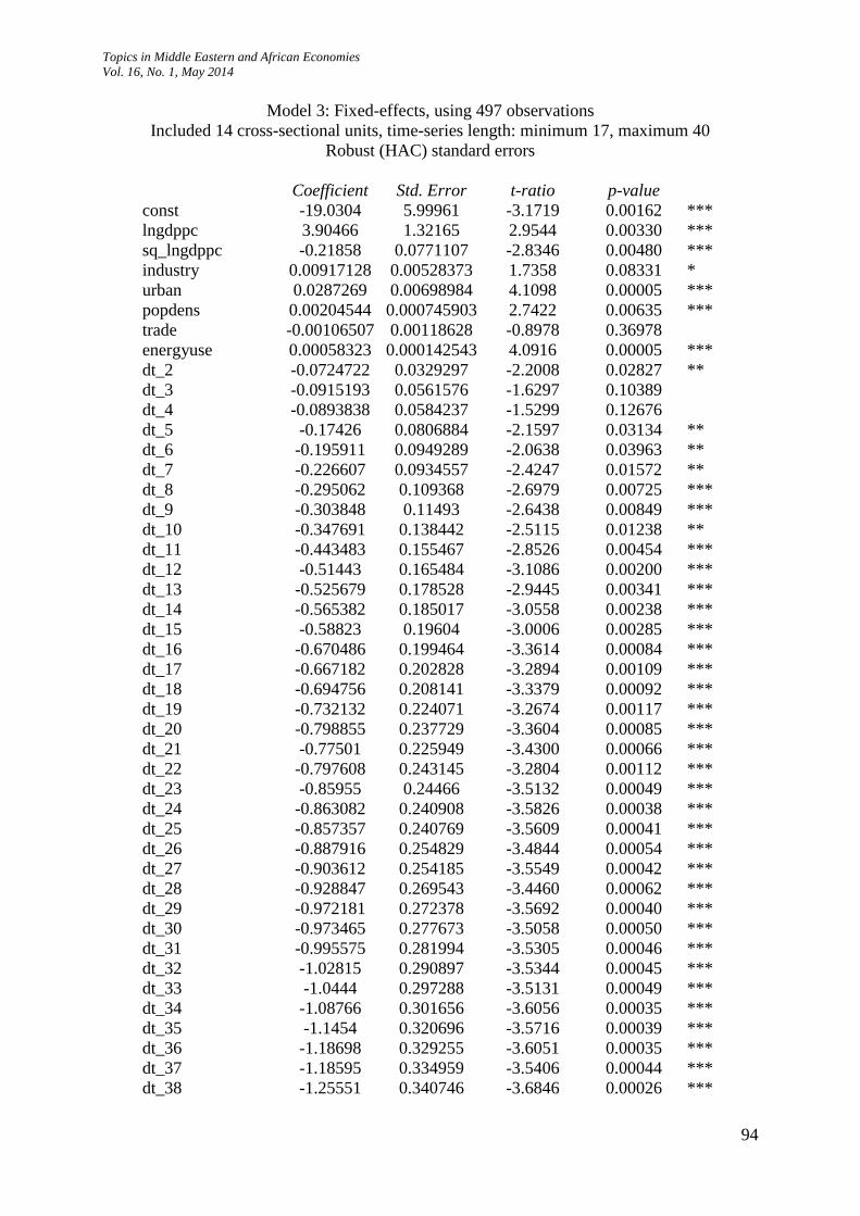
Since the cubic form equation turns out to have insignificant coefficients for lngdppc,

sq_lngdppc and tr_lngdppc, once other variables are controlled for in Model 2, we attempt to


Vol. 16, No. 1, May 2014

82

run a quadratic regression to see whether there is an EKC relationship in case the controls are

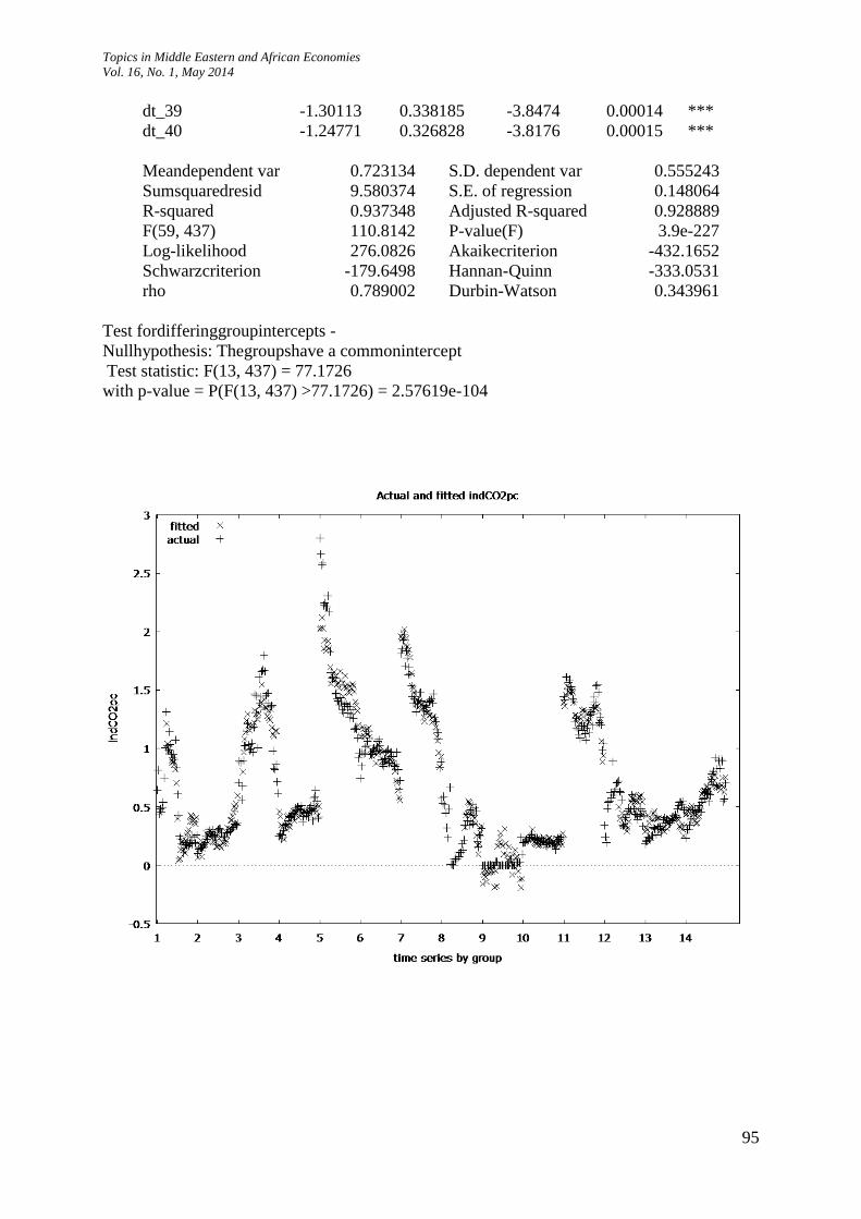
added together with time dummies. Model 3 reports the results from the quadratic form

equation, where an inverted-U relationship is detected between per capita income and

industrial emissions (see the third column in Table 2). This supports the EKC hypothesis for

the countries selected and the turning point per capita GDP (exp (- )) corresponds to

around 7,570 international dollars (at 2005 constant prices). This finding implies that some

countries like Albania, Algeria, Egypt, Morocco, Syria and Tunisia have not reached the

turning point income where their industrial emissions will start to decline, whereas some like

Cyprus, France, Greece, Italy and Spain have already been enjoying the downward sloping

portion of the EKC. On the other hand, some countries, including Turkey, reached the turning

point around the mid-1990s.

What is more, the positive effects of industry, urbanization, population density and energy use

are proven to be robust in the last specification as well. Trade intensity, on the other hand,

appears to be insignificant. In sum, one could easily note that the selected Mediterranean

countries have experienced an EKC relationship for industrial CO2 emissions or will enjoy a

reduction in their industrial pollution as their per capita income rises at some point in time

depending on their characteristics related to industrial shares of total output, urban population,

population density and the amount of energy use.

Most of these findings are in line with the previous studies that study industrial or total CO2

emissions. Income per capita has usually been evidenced as a major factor that manipulates

industrial emissions. Most of the EKC literature supports this finding for income. Needless to

say, the shape of the relationship depends on the country, country group or time period

investigated.


Vol. 16, No. 1, May 2014

83

Environmental pollution tends to increase when economies switch from agriculture to

industry; hence increases in industrial share of GDP are expected to worsen environmental

degradation. The effect is also valid during the transition from industry to services and

knowledge-based sectors. As manufacturing and construction value-added shares decline,

industrial CO2 emissions are found to decline in many studies (Panayotou, 1993; Komen et

al., 1997; Vukina et al., 1999; Hettige et al., 2000).

In the pace of economic development, the move from rural to urban areas is almost inevitable.

This trend is expected to increase environmental pollution since economic activity mostly

takes place in urbanized areas and higher urban consumption leads to a higher demand for

energy and resources. For instance, economic development has been associated with higher

levels of urbanization and higher industrial emissions in China in a study that examines the

period 1995-2009 (Zhou et al., 2012). Our results also confirm this phenomenon with a

positive impact on industrial per capita CO2 emissions.

Population pressure is found to be another contributing factor to increased CO2 emissions.

Several other studies also claim the same effect for population density (Grossman and

Krueger, 1991; Panayotou, 1997). This translates into an environmental threat of increasing

world population on emissions, although all other factors remain constant and the EKC

relationship holds with a turning point of income.

In our analysis, the share of total trade in GDP, namely trade density, does not display a

significant sign. What would be more convenient to mark here could be trade composition of

economies instead of simply looking at the sum of exports and imports. For instance, the

“pollution haven” hypothesis suggests that industries that pollute more would relocate their

activities in countries where environmental regulations are less strict or do not exist at all.

Hence, if a country starts importing the most polluting goods from other countries or regions,


Vol. 16, No. 1, May 2014

84

one would expect that industrial emissions would become lower, although the trade volume

changes. Our study falls short of explaining these details for now.

Regarding the impact of energy use on industrial CO2 emissions, IEA (2007: 20) reports that

industrial energy use has been boosted importantly in recent decades with a different rate of

growth in each sector. Sectors like chemicals, petrochemicals, cement, iron and steel have

been consuming large amounts of energy, mostly fossil fuels, in expanding economies and

this energy use has brought together higher dependence on fossil fuels. Country studies have

also proven the fact that energy use is responsible for emissions increases. For instance, Lim

et al. (2009) find that the energy sector is a major contributor to industrial emissions in Korea

for the period 1990-2003 since the recent economic growth has largely gone along with

increasing energy consumption in the economy. Krey et al. (2012) find evidence of the same

impact on industrial CO2 emissions for Chinese energy consumption growth together with

total output increase. On the other hand, these findings imply that a structural shift from

energy-intensive sectors towards services sectors would bring together a reduction in

emissions.

These results offer hints to cope with the environmental effects of economic growth using

appropriate policy tools related to population distribution, urbanization, industrialization and

energy use.

5. Conclusion

Industry is a highly energy-intensive sector, intensively using fossil fuels, where carbon

emissions from industry are dominated by the production of goods in certain sectors such as

iron and steel, cement and chemicals and petrochemicals. Increasing activity in these sectors


Vol. 16, No. 1, May 2014

85

leads to further exploitation of fossil fuels and a rise in CO2 emissions. Neither the level of

energy use of the industry sector nor the type of energy used by the sector is expected to

change significantly in the near future.

The environment of the Mediterranean region appears to be one of richest; but also, due to the

intensity of trade and industry, one of the most vulnerable in the world. This fact makes

national and supranational policies designed against environmental degradation a priority for

the countries of the region. In this context, this paper examined the effects of GDP per capita,

value added of industry, urban population, population density, trade intensity and energy use

on CO2 emissions from manufacturing industries and construction containing emissions from

combustion of fuels in industry by employing panel fixed-effects estimations.

The analyses show that there is a tilted-S shaped relationship between GDP per capita and per

capita industrial CO2 emissions. But the S-curve relationship disappears once other

explanatory factors such as industrial value added, urbanization, energy use and population

dynamics are accounted for. However, a quadratic regression shows the existence of an EKC

relationship even in the presence of control variables. Also the analysis using a quadratic

regression detects the positive relation of per capita industrial CO2 emissions with value

added of industry, urban population, population density and energy use. Thus, the quadratic

regression confirms that pollution tends to decrease in the selected Mediterranean countries

after they reach a certain level of per capita GDP. However, this decreasing trend faces a risk

of reversal in the absence of appropriate urban, industrial and energy policies. The analysis

sets forth that the development of the tertiary sector in the region and the decrease in the

relative contribution of the industrial sectors to the economy is expected to alleviate pollution.

In addition, policies aimed at reducing rural-to-urban migration, and thus population density

in urban areas, and the building of an energy policy based on the use of less fossil fuels appear


Vol. 16, No. 1, May 2014

86

as the policy priorities in order to enjoy the negatively-sloped part of the EKC in the

Mediterranean region.

References

Antweiler, W., Copeland, B. R., Taylor, M. S., 2001. Is free trade good for the environment.

American Economic Review, 91: 877–908.

Arellano, M., 2003. Panel Data Econometrics, Oxford: Oxford University Press.

Baltagi, B. H., 2005. Econometric Analysis of Panel Data, 3rd edition, John Wiley & Sons

Ltd., West Sussex, England.

Brown, J.H., Barnosky, A.D., Hadly, E.A., Bascompte, J., Berlow, E.L., Fortelius, M., and

Getz, W.M., 2012. "Approaching a state shift in Earth/'s biosphere." Nature 486(7401): 52-58.

Benoit, G. and Comeau, A., 2005. A Sustainable Future for the Mediterranean: The Blue

Plan's Environment and Development Outlook, Earthscan Publications, France

Blacksmith Institute. 2012. The World’s Worst Pollution Problems: Assessing Health Risks at

Hazardous Waste Sites, Blacksmith Institute and Green Cross Switzerland, New York

Cole, M.A., Rayner, A.J., Bates, J.M., 1997. The Environmental Kuznets Curve: an empirical

analysis. Environment and Development Economics, 2: 401– 416.

Cropper, M., Griffiths, C., 1994. The interaction of populations, growth and environmental

quality. American Economic Review, 84: 250– 254.

Dasgupta, S., Laplante, B., Wang, H., Wheeler, D., 2002. Confronting the Environmental

Kuznets Curve. Journal of Economic Perspectives, 16 (1): 147–168.

Dasgupta, S., Mody, A., Roy, S., Wheeler, D., 2001. Environmental regulation and

development: a cross-country empirical analysis. Oxford Development Studies, 29 (2): 173–

187.

Dinda, S., 2004. Environmental Kuznets Curve Hypothesis: A Survey. Ecological Economics,

49: 431– 455

ExxonMobil, 2013.The Outlook for Energy: A View to 2040. ExxonMobil, Texas

European Commission, 2006. Establishing an Environmental Strategy for the Mediterranean,

SEC (2006) 1082, Brussels


Vol. 16, No. 1, May 2014

87

Grossman, G. M., & Krueger, A. B. 1991. Environmental impacts of a North American Free

Trade Agreement. National Bureau of Economic Research Working Paper 3914, NBER,

Cambridge MA.

Grossman, G.M. and Krueger, A.B., 1995. Economic growth and the environment. Quarterly

Journal of Economics 110 (2): 353– 377.

Hettige, H., Mani, M., Wheeler, D., 2000. Industrial pollution in economic development: the

environmental Kuznets curve revisited Journal of Development Economics, 62: 445–476

Holtz-Eakin, D., Selden, T.M., 1995. Stoking the fires?: CO2 emissions and economic

growth. Journal of Public Economics, 57: 85–101.

IEA, 2010. Energy Technology Perspectives 2010: Scenarios and Strategies to 2050. IEA

(International Energy Agency): Paris.

IEA, 2012. CO2 Emissions from Fuel Combustion 2012:Highlights. IEA (International

Energy Agency): Paris.

Komen, R., Gerking, S., Folmer, H., 1997. Income and environmental R&D: empirical

evidence from OECD countries. Environment and Development Economics 2, 505–515.

Krey, V., O'Neill, B. C., van Ruijvenb, B. Chaturvedi, V., Daioglouc, V., Eom, J., Jiang, L.,

Nagai, Y., Pachauri, S. and Ren, X., 2012. Urban and rural energy use and carbon dioxide

emissions in Asia. Energy Economics (The Asia Modeling Exercise: Exploring the Role of

Asia in Mitigating Climate Change), 34, Supplement 3: S272–S283.

Kuznets, P. and Simon, P., 1955. Economic growth and income inequality. American

Economic Review, 45: 1– 28.

Lim, H. J., Yoo, S. H. and Kwak, S. J., 2009. Industrial CO2 emissions from energy use in

Korea: A structural decomposition analysis. Energy Policy, 37 (2): 686–698

Meadows, D.H., Meadows, D.L., Randers, J., Behrens, W., 1972.The Limits to Growth.

Universe Books, New York.

McConnell, K. E. 1997. Income and the demand for environmental quality. Environment and

Development Economics, 2(4), 383-399.

Mundlak, Y., 1978.On the pooling of time series and cross-section data. Econometrica 46:

69–85.

Panayotou, T., 1993. Empirical tests and policy analysis of environmental degradation at

different stages of economic development. Working Paper WP238, Technology and

Employment Programme, International Labour Office, Geneva.

Panayotou, T., 1997. Demystifying the environmental Kuznets curve: Turning a black box

into a policy tool. Environment and Development Economics, 2: 465–484.


Vol. 16, No. 1, May 2014

88

Panayotou, T., 1999. The economics of environments in transition. Environment and

Development Economics, 4 (4): 401– 412.

Ren, X., Krey, V., O'Neill, B.C., van Ruijven, B., Chaturvedi, V., Daioglou, V., Eom, J.,

Jiang, L., Nagai, Y., and Pachauri, S. 2012. Urban and rural energy use and carbon dioxide

emissions in Asia. Energy economics 34: 272-S283.

Selden, T. and Song, D., 1995. Neoclassical growth, the J Curve for abatement, and the

inverted-U Curve for pollution. Journal of Environmental Economics and Management, 29:

162– 168.

Shafik, N., 1994. Economic development and environmental quality: an econometric analysis.

Oxford Economic Papers, 46: 757– 773.

Shafik, N. and Bandyopadhyay, S., 1992. Economic growth and environmental quality: time

series and cross-country evidence. Background Paper for the World Development Report. The

World Bank, Washington, DC.

Stern, D. I., 1998. Progress on the environmental Kuznets curve? Environment and

Development Economics, 3: 173–196.

Stern, D. I., 2004. The Rise and Fall of the Environmental Kuznets Curve. World

Development, 32 (8): 1419–1439

Torras, M., Boyce, J.K., 1998. Income, inequality, and pollution: a reassessment of the

Environmental Kuznets Curve. Ecological Economics, 25: 147– 160.

UNEP/MAP, 2012. State of the Mediterranean Marine and Coastal Environment,

UNEP/MAP-Barcelona Convention, Athens.

Vukina, T., Beghin, J.C., Solakoglu, E.G., 1999. Transition to markets and the environment:

effects of the change in the composition of manufacturing output. Environment and

Development Economics, 4 (4): 582– 598.

Wheeler, D., 2000. Racing to the bottom? Foreign investment and air pollution in developing

countries. World Bank Development Research Group Working Paper no. 2524.

World Bank. 2013. World Development Indicators.

Zhou, X., Zhang, J. Li, J., 2012. Industrial structural transformation and carbon dioxide

emissions in China, Energy Policy, In Press.Accepted 11 July 2012.


Vol. 16, No. 1, May 2014

89

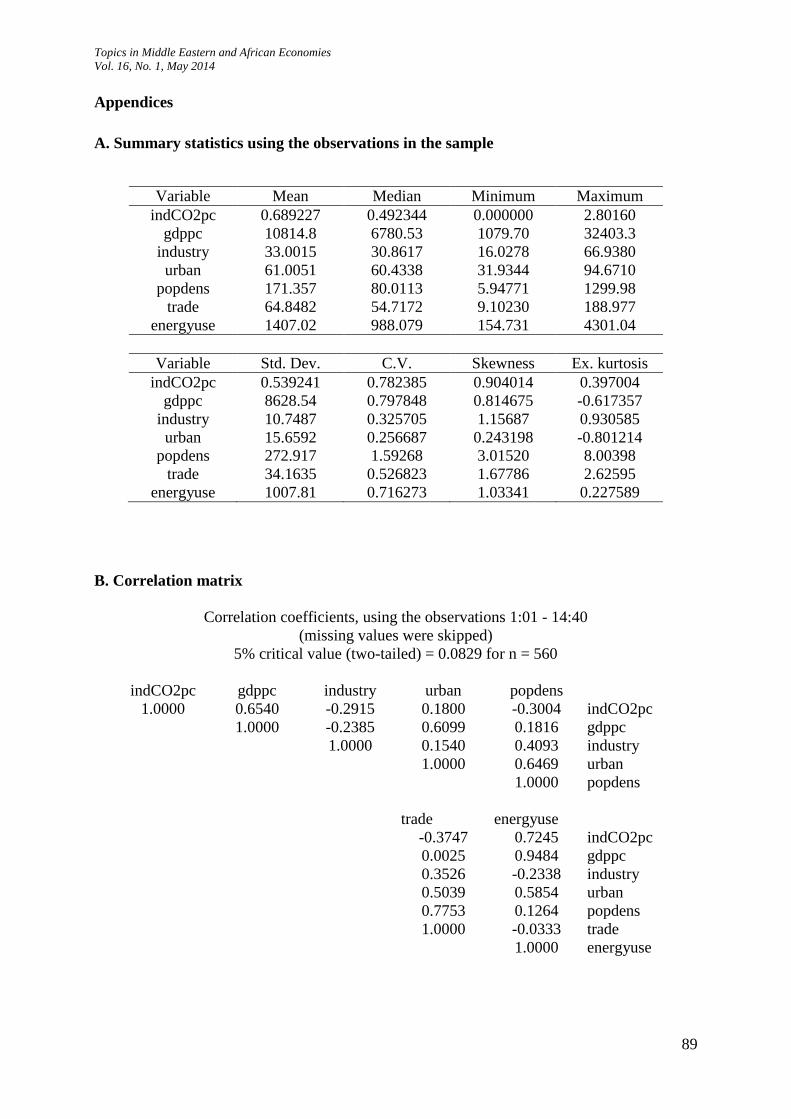
Appendices

A. Summary statistics using the observations in the sample

Variable Mean Median Minimum Maximum

indCO2pc 0.689227 0.492344 0.000000 2.80160

gdppc 10814.8 6780.53 1079.70 32403.3

industry 33.0015 30.8617 16.0278 66.9380

urban 61.0051 60.4338 31.9344 94.6710

popdens 171.357 80.0113 5.94771 1299.98

trade 64.8482 54.7172 9.10230 188.977

energyuse 1407.02 988.079 154.731 4301.04

Variable Std. Dev. C.V. Skewness Ex. kurtosis

indCO2pc 0.539241 0.782385 0.904014 0.397004

gdppc 8628.54 0.797848 0.814675 -0.617357

industry 10.7487 0.325705 1.15687 0.930585

urban 15.6592 0.256687 0.243198 -0.801214

popdens 272.917 1.59268 3.01520 8.00398

trade 34.1635 0.526823 1.67786 2.62595

energyuse 1007.81 0.716273 1.03341 0.227589

B. Correlation matrix

Correlation coefficients, using the observations 1:01 - 14:40

(missing values were skipped)

5% critical value (two-tailed) = 0.0829 for n = 560

indCO2pc gdppc industry urban popdens

1.0000 0.6540 -0.2915 0.1800 -0.3004 indCO2pc

1.0000 -0.2385 0.6099 0.1816 gdppc

1.0000 0.1540 0.4093 industry

1.0000 0.6469 urban

1.0000 popdens

trade energyuse

-0.3747 0.7245 indCO2pc

0.0025 0.9484 gdppc

0.3526 -0.2338 industry

0.5039 0.5854 urban

0.7753 0.1264 popdens

1.0000 -0.0333 trade

1.0000 energyuse


Vol. 16, No. 1, May 2014

90

C. Regression Outputs and Fitted Plots

Model 1: Fixed-effects, using 560 observations

Included 14 cross-sectional units, time-series length = 40

Robust (HAC) standard errors

Coefficient Std. Error t-ratio p-value

const 84.0032 38.02 2.2094 0.02759 **

lngdppc -30.7727 13.6029 -2.2622 0.02411 **

sq_lngdppc 3.7082 1.60838 2.3055 0.02154 **

tr_lngdppc -0.145948 0.0628383 -2.3226 0.02060 **

dt_2 -0.00544326 0.0229316 -0.2374 0.81247

dt_3 -0.00994076 0.035364 -0.2811 0.77875

dt_4 -0.00357978 0.0325945 -0.1098 0.91259

dt_5 -0.0492273 0.0507697 -0.9696 0.33270

dt_6 -0.00683056 0.0613945 -0.1113 0.91146

dt_7 -0.03237 0.057558 -0.5624 0.57410

dt_8 -0.0208813 0.0613249 -0.3405 0.73362

dt_9 0.0556157 0.0688846 0.8074 0.41983

dt_10 -0.00939058 0.0681988 -0.1377 0.89054

dt_11 -0.0924861 0.0775096 -1.1932 0.23334

dt_12 -0.107845 0.0899597 -1.1988 0.23116

dt_13 -0.102276 0.0952806 -1.0734 0.28360

dt_14 -0.118631 0.0946348 -1.2536 0.21058

dt_15 -0.146126 0.0941307 -1.5524 0.12120

dt_16 -0.164823 0.0996172 -1.6546 0.09864 *

dt_17 -0.135326 0.102255 -1.3234 0.18630

dt_18 -0.124931 0.100013 -1.2492 0.21219

dt_19 -0.0961955 0.100024 -0.9617 0.33665

dt_20 -0.149683 0.0988412 -1.5144 0.13056

dt_21 -0.121822 0.0968989 -1.2572 0.20926

dt_22 -0.170106 0.0961709 -1.7688 0.07753 *

dt_23 -0.198548 0.107937 -1.8395 0.06643 *

dt_24 -0.185094 0.111505 -1.6600 0.09754 *

dt_25 -0.167691 0.113613 -1.4760 0.14057

dt_26 -0.172286 0.120605 -1.4285 0.15376

dt_27 -0.159969 0.119076 -1.3434 0.17974

dt_28 -0.168551 0.112632 -1.4965 0.13516

dt_29 -0.181072 0.11707 -1.5467 0.12256

dt_30 -0.162542 0.122464 -1.3273 0.18502

dt_31 -0.1611 0.117139 -1.3753 0.16965

dt_32 -0.183771 0.120848 -1.5207 0.12897

dt_33 -0.162559 0.126425 -1.2858 0.19910

dt_34 -0.196126 0.132624 -1.4788 0.13982

dt_35 -0.229117 0.140855 -1.6266 0.10444

dt_36 -0.273983 0.142209 -1.9266 0.05459 *

dt_37 -0.268336 0.148194 -1.8107 0.07078 *

dt_38 -0.330125 0.149419 -2.2094 0.02760 **

dt_39 -0.424241 0.161535 -2.6263 0.00889 ***

dt_40 -0.40183 0.159543 -2.5186 0.01209 **


Vol. 16, No. 1, May 2014

91

Meandependent var 0.689227 S.D. dependent var 0.539241

Sumsquaredresid 18.79436 S.E. of regression 0.193107

R-squared 0.884375 Adjusted R-squared 0.871758

F(55, 504) 70.08972 P-value(F) 2.5e-201

Log-likelihood 155.8208 Akaikecriterion -199.6416

Schwarzcriterion 42.72286 Hannan-Quinn -105.0045

rho 0.837947 Durbin-Watson 0.274000

Test fordifferinggroupintercepts -

Nullhypothesis: Thegroupshave a commonintercept

Test statistic: F(13, 504) = 123.164

with p-value = P(F(13, 504) > 123.164) = 4.72466e-147


Vol. 16, No. 1, May 2014

92


Included 14 cross-sectional units, time-series length: minimum 17, maximum 40



const -1.97035 38.6503 -0.0510 0.95937

lngdppc -1.9765 13.8188 -0.1430 0.88633

sq_lngdppc 0.459354 1.64379 0.2794 0.78003

tr_lngdppc -0.0258854 0.0647798 -0.3996 0.68965

industry 0.00912292 0.00538928 1.6928 0.09121 *

urban 0.0260708 0.00690339 3.7765 0.00018 ***

popdens 0.00188558 0.000690107 2.7323 0.00655 ***

trade -0.00115261 0.00106084 -1.0865 0.27786

energyuse 0.000585649 0.000144734 4.0464 0.00006 ***

dt_2 -0.070975 0.0314233 -2.2587 0.02440 **

dt_3 -0.0885041 0.0510695 -1.7330 0.08380 *

dt_4 -0.0843342 0.0487784 -1.7289 0.08453 *

dt_5 -0.169409 0.0720978 -2.3497 0.01923 **

dt_6 -0.190687 0.0851836 -2.2385 0.02569 **

dt_7 -0.217955 0.079122 -2.7547 0.00612 ***

dt_8 -0.285259 0.0959016 -2.9745 0.00310 ***

dt_9 -0.291172 0.0980068 -2.9709 0.00313 ***

dt_10 -0.331614 0.117414 -2.8243 0.00496 ***

dt_11 -0.426187 0.13164 -3.2375 0.00130 ***

dt_12 -0.494803 0.141189 -3.5045 0.00050 ***

dt_13 -0.50398 0.148402 -3.3960 0.00075 ***

dt_14 -0.541602 0.154507 -3.5054 0.00050 ***

dt_15 -0.561578 0.160401 -3.5011 0.00051 ***

dt_16 -0.642767 0.170366 -3.7729 0.00018 ***

dt_17 -0.637739 0.170454 -3.7414 0.00021 ***

dt_18 -0.662155 0.174068 -3.8040 0.00016 ***

dt_19 -0.69732 0.188929 -3.6909 0.00025 ***

dt_20 -0.762137 0.20051 -3.8010 0.00016 ***

dt_21 -0.73695 0.18498 -3.9839 0.00008 ***

dt_22 -0.758073 0.197745 -3.8336 0.00014 ***

dt_23 -0.819725 0.202082 -4.0564 0.00006 ***

dt_24 -0.820292 0.193362 -4.2423 0.00003 ***

dt_25 -0.812952 0.189035 -4.3005 0.00002 ***

dt_26 -0.842408 0.202759 -4.1547 0.00004 ***

dt_27 -0.856491 0.203512 -4.2086 0.00003 ***

dt_28 -0.880098 0.213142 -4.1292 0.00004 ***

dt_29 -0.921138 0.215499 -4.2744 0.00002 ***

dt_30 -0.919265 0.216717 -4.2418 0.00003 ***

dt_31 -0.939258 0.221433 -4.2417 0.00003 ***

dt_32 -0.970352 0.228084 -4.2544 0.00003 ***

dt_33 -0.985341 0.236668 -4.1634 0.00004 ***

dt_34 -1.02677 0.236624 -4.3393 0.00002 ***

dt_35 -1.0828 0.254631 -4.2524 0.00003 ***

dt_36 -1.12194 0.263493 -4.2580 0.00003 ***

dt_37 -1.11867 0.267801 -4.1773 0.00004 ***


Vol. 16, No. 1, May 2014

93

dt_38 -1.18741 0.267302 -4.4422 0.00001 ***

dt_39 -1.23492 0.260467 -4.7412 <0.00001 ***

dt_40 -1.18199 0.254763 -4.6395 <0.00001 ***




F(60, 436) 109.1016 P-value(F) 2.0e-226


Schwarzcriterion -175.0822 Hannan-Quinn -331.0422




Test statistic: F(13, 436) = 64.1591

with p-value = P(F(13, 436) >64.1591) = 1.63163e-092


Vol. 16, No. 1, May 2014

94


Included 14 cross-sectional units, time-series length: minimum 17, maximum 40



const -19.0304 5.99961 -3.1719 0.00162 ***

lngdppc 3.90466 1.32165 2.9544 0.00330 ***

sq_lngdppc -0.21858 0.0771107 -2.8346 0.00480 ***

industry 0.00917128 0.00528373 1.7358 0.08331 *

urban 0.0287269 0.00698984 4.1098 0.00005 ***

popdens 0.00204544 0.000745903 2.7422 0.00635 ***

trade -0.00106507 0.00118628 -0.8978 0.36978

energyuse 0.00058323 0.000142543 4.0916 0.00005 ***

dt_2 -0.0724722 0.0329297 -2.2008 0.02827 **

dt_3 -0.0915193 0.0561576 -1.6297 0.10389

dt_4 -0.0893838 0.0584237 -1.5299 0.12676

dt_5 -0.17426 0.0806884 -2.1597 0.03134 **

dt_6 -0.195911 0.0949289 -2.0638 0.03963 **

dt_7 -0.226607 0.0934557 -2.4247 0.01572 **

dt_8 -0.295062 0.109368 -2.6979 0.00725 ***

dt_9 -0.303848 0.11493 -2.6438 0.00849 ***

dt_10 -0.347691 0.138442 -2.5115 0.01238 **

dt_11 -0.443483 0.155467 -2.8526 0.00454 ***

dt_12 -0.51443 0.165484 -3.1086 0.00200 ***

dt_13 -0.525679 0.178528 -2.9445 0.00341 ***

dt_14 -0.565382 0.185017 -3.0558 0.00238 ***

dt_15 -0.58823 0.19604 -3.0006 0.00285 ***

dt_16 -0.670486 0.199464 -3.3614 0.00084 ***

dt_17 -0.667182 0.202828 -3.2894 0.00109 ***

dt_18 -0.694756 0.208141 -3.3379 0.00092 ***

dt_19 -0.732132 0.224071 -3.2674 0.00117 ***

dt_20 -0.798855 0.237729 -3.3604 0.00085 ***

dt_21 -0.77501 0.225949 -3.4300 0.00066 ***

dt_22 -0.797608 0.243145 -3.2804 0.00112 ***

dt_23 -0.85955 0.24466 -3.5132 0.00049 ***

dt_24 -0.863082 0.240908 -3.5826 0.00038 ***

dt_25 -0.857357 0.240769 -3.5609 0.00041 ***

dt_26 -0.887916 0.254829 -3.4844 0.00054 ***

dt_27 -0.903612 0.254185 -3.5549 0.00042 ***

dt_28 -0.928847 0.269543 -3.4460 0.00062 ***

dt_29 -0.972181 0.272378 -3.5692 0.00040 ***

dt_30 -0.973465 0.277673 -3.5058 0.00050 ***

dt_31 -0.995575 0.281994 -3.5305 0.00046 ***

dt_32 -1.02815 0.290897 -3.5344 0.00045 ***

dt_33 -1.0444 0.297288 -3.5131 0.00049 ***

dt_34 -1.08766 0.301656 -3.6056 0.00035 ***

dt_35 -1.1454 0.320696 -3.5716 0.00039 ***

dt_36 -1.18698 0.329255 -3.6051 0.00035 ***

dt_37 -1.18595 0.334959 -3.5406 0.00044 ***

dt_38 -1.25551 0.340746 -3.6846 0.00026 ***


Vol. 16, No. 1, May 2014

95

dt_39 -1.30113 0.338185 -3.8474 0.00014 ***

dt_40 -1.24771 0.326828 -3.8176 0.00015 ***




F(59, 437) 110.8142 P-value(F) 3.9e-227


Schwarzcriterion -179.6498 Hannan-Quinn -333.0531




Test statistic: F(13, 437) = 77.1726

with p-value = P(F(13, 437) >77.1726) = 2.57619e-104

economic development and industrial pollution in...

Documents