econ4150 - introductory econometrics lecture 15 ... · econ4150 - introductory econometrics lecture...
TRANSCRIPT

ECON4150 - Introductory Econometrics
Lecture 15: Introduction to time series
Monique de Haan([email protected])
Stock and Watson Chapter 14.1-14.6

2
Lecture outline
• What is time series data
• Estimating a causal effect vs forecasting
• Lags, first differences and growth rates
• Autocorrelation
• Autoregressions
• Auto regressive distributed lag model
• Nonstationarity: stochastic trends
• random walk with and without drift• testing for stochastic trends (Dickey-Fuller test)

3
What is time series data?
Cross section data is data collected for multiple entities at one point in time
Panel data is data collected for multiple entities at multiple points in time
Time series data is data collected for a single entity at multiple points in time
• Yearly GDP of Norway for a period of 20 years
• Daily NOK/Euro exchange rate for past year
• Quarterly data on the inflation & unemployment rate in the U.S from1957-2005

4
What is time series data?
Quarterly time series data on inflation for the U.S. from 1957 to 2005
0
5
10
15
Infla
tion
(%)
1957q1 1969q1 1981q1 1993q1 2005q1
time
5
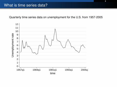
What is time series data?
Quarterly time series data on unemployment for the U.S. from 1957-2005
0
1
2
3
4
5
6
7
8
9
10
11
12
Une
mpl
oym
ent r
ate
1957q1 1969q1 1981q1 1993q1 2005q1
time

6
What is time series data?
Quarterly data on inflation & unemployment in the U.S. 2000-2005:

7
What is time series data?
• A particular observation Yt indexed by subscript t
• Total number of observations equals T
• Yt is current value and value in previous period is Yt−1 (first lag)
• In general Yt−j is called j th lag and similarly, Yt+j is the j th future value
• The first difference Yt − Yt−1 is the change in Y from period t − 1 toperiod t
• Time series regression models can be used for
• (1) estimating (dynamic) causal effects;
• (2) forecasting

8
Estimating (dynamic) causal effect vs forecasting
• Time series data is often used for forecasting
• For example next year’s economic growth is forecasted based onpast and current values of growth & other (lagged) explanatoryvariables
• Forecasting is quite different from estimating causal effects and isgenerally based on different assumptions.
• Models that are useful for forecasting need not have a causalinterpretation!
• OLS coefficients need not be unbiased & consistent
• Measures of fit, such as the (adjusted) R2 or the SER
• are not very informative when estimating causal effects
• are informative about the quality of a forecasting model

9
Logarithms and growth rates
• Suppose that Yt is some time series, then the rate of growth of Y is
Yt − Yt−1
Yt−1=4Yt
Yt−1
• instead, we often use the “logarithmic growth" or “log-difference":
4lnYt = ln (Yt)− ln (Yt−1)
= ln(
YtYt−1
)= ln
(Yt
Yt−1+
Yt−1Yt−1− Yt−1
Yt−1
)= ln
(1 +
Yt−Yt−1Yt−1
)≈ 4Yt
Yt−1
see also formula (8.16) of S&W

10
Example: inflation in the U.S.
Annualized rate of inflation:
inflationt ∼= 100× 4× (ln (Yt)− ln (Yt−1))
Stata:tsset timegen ln_CPI=ln(CPI)gen ln_CPI_1stlag=ln(L1.CPI)gen inflation=400*( ln(CPI) - ln(L1.CPI) )
time CPI ln_CPI ln_CPI_1stlag inflation
t Yt ln (Yt ) ln (Yt−1) 400 · (ln (Yt )− ln (Yt−1))
1957q1 27.77667 3.32419631957q2 28.01333 3.3326806 3.3241963 3.39371281957q3 28.26333 3.3415654 3.3326806 3.5538941957q4 28.4 3.3463891 3.3415654 1.92951031958q1 28.73667 3.3581739 3.3463891 4.71389081958q2 28.93 3.3648791 3.3581739 2.68210831958q3 28.91333 3.3643029 3.3648791 -0.230504181958q4 28.94333 3.3653399 3.3643029 0.41480139

11
Autocorrelation
In time series data, Yt is typically correlated with Yt−j , this is calledautocorrelation or serial correlation
• The j thautocovariance=Cov(Yt ,Yt−j) can be estimated by
Cov(Yt ,Yt−j) =1T
T∑t=j+1
(Yt − Y j+1,T
)(Yt−j − Y 1,T−j
)Y j+1,T is the sample average of Y computed over observations t = j + 1, ...,T
Y 1,T−j is the sample average of Y computed over observations t = 1, ...,T − j
• The j thautocorrelation= ρj =Cov(Yt ,Yt−j )
Var(Yt )can be estimated by
ρj =Cov(Yt ,Yt−j)
Var (Yt)
• j start-up observations are lost in constructing these sample statistics
• denominator of j thautocorrelation assumes stationarity of Yt , whichimplies (among other things) Var (Yt) = Var (Yt−j)

12
Autocorrelation
First 4 autocorrelations of inflation (inft ):
Tuesday April 15 15:38:55 2014 Page 1
___ ____ ____ ____ ____(R) /__ / ____/ / ____/ ___/ / /___/ / /___/ Statistics/Data Analysis
1 . corrgram inflation if tin(1960q1,2004q4), noplot lags(4)
LAG AC PAC Q Prob>Q
1 0.8359 0.8361 127.89 0.0000 2 0.7575 0.1937 233.49 0.0000 3 0.7598 0.3206 340.34 0.0000 4 0.6699 -0.1881 423.87 0.0000
First 4 autocorrelations of the change in inflation (4inft = inft − inft−1):
Tuesday April 15 15:41:16 2014 Page 1
___ ____ ____ ____ ____(R) /__ / ____/ / ____/ ___/ / /___/ / /___/ Statistics/Data Analysis
1 . corrgram D.inflation if tin(1960q1,2004q4), noplot lags(4)
LAG AC PAC Q Prob>Q
1 -0.2618 -0.2636 12.548 0.0004 2 -0.2549 -0.3497 24.507 0.0000 3 0.2938 0.1461 40.481 0.0000 4 -0.0605 -0.0220 41.162 0.0000

13
Stationarity
• The denominator of j thautocorrelation assumes stationarity of Yt
• A time series Yt is stationary if its probability distribution does notchange over time,
• when the joint distribution of (Ys+1, ...,YS+T ) does not depend on s
• Stationarity implies that Y1 has the same distribution as Yt for anyt = 1, 2, ...
• In other words, {Y1,Y2, ...,YT} are identically distributed, however, theyare not necessarily independent!
• If a series is nonstationary, then convential hypothesis tests, confidenceintervals and forecasts can be unreliable.
• Stationarity says that history is relevant, it is a key requirement forexternal validity of time series regression.

14
First order autoregressive model: AR(1)
• Suppose we want to forecast the change in inflation from this quarter tothe next
• When predicting the future of a time series a good place start is in theimmediate past.
• The first order autoregressive model (AR(1))
Yt = β0 + β1Yt−1 + ut
• Forecast in next period based on AR(1) model:
YT+1|T = β0 + β1YT
• Forecast error is the mistake made by the forecast
Forecast error = YT+1 − YT+1|T

15
Forecast vs predicted value & forecast error vs residual
• A forecast is not the same as a predicted value
• A forecast error is not the same as a residual
OLS predicted values Yt and residuals ut = Yt−Yt for t ≤ T are “in-sample”:
• They are calculated for the observations in the sample used to estimatethe regression.
• Yt is observed in the data set used to estimate the regression.
A forecast YT+j|T and forecast error YT+j − YT+j|T for j ≥ 1 are“out-of-sample”:
• They are calculated for some date beyond the data set used to estimatethe regression.
• YT+j is not observed in the data set used to estimate theregression.

16
First order autoregressive model: AR(1)
4inflationt = β0 + β14inflationt−1 + ut
Friday April 11 14:58:54 2014 Page 1
___ ____ ____ ____ ____(R) /__ / ____/ / ____/ ___/ / /___/ / /___/ Statistics/Data Analysis
> gen d_inflation=D1.inflation(2 missing values generated)
1 . regress d_inflation L1.d_inflation if tin(1962q1,2004q4), r
Linear regression Number of obs = 172 F( 1, 170) = 6.08 Prob > F = 0.0146 R-squared = 0.0564 Root MSE = 1.664
Robust d_inflation Coef. Std. Err. t P>|t| [95% Conf. Interval]
d_inflation L1. -.2380471 .0965017 -2.47 0.015 -.4285431 -.047551 _cons .0171008 .1268849 0.13 0.893 -.2333721 .2675736
2 . dis "Adjusted Rsquared = " _result(8)Adjusted Rsquared = .05082857
• 4inf 2005q1|2004q4 = 0.017− 0.238 · 4inf2004q4 = −0.43
• Forecast error = 4inf2005q1 − 4inf 2005q1|2004q4 = −1.14− (−0.43) = −0.71

17
Root mean squared forecast error
• Forecasts are uncertain and the Root Mean Squared Forecast Error(RMSFE) is a measure of forecast uncertainty.
• The RMSFE is a measure of the spread of the forecast error distribution.
RMSFE =
√E[(
YT+1 − YT+1|T
)2]
• The RMSFE has two sources of error:
1 The error arising because future values of ut are unknown
2 The error in estimating the coefficients β0 and β1
• If the sample size is large the first source of error will be larger than thesecond and RMSFE ≈
√Var (ut)
•√
Var (ut) can be estimated by the SER = 1T−2
∑Tt=1 u2
t .

18
AR(p) model
The pth order autoregressive model (AR(p)) is
Yt = β0 + β1Yt−1 + β2Yt−2 + ...+ βpYt−p + ut
• The AR(p) model uses p lags of Y as regressors
• The number of lags p is called the order or lag length of theautoregression.
• The coefficients generally do not have a causal interpretation.
• We can use t- or F-tests to determine the lag order p
• Or we can determine p using an “information criterion” (more on thislater. . . )

19
AR(4)
Friday April 11 15:02:06 2014 Page 1
___ ____ ____ ____ ____(R) /__ / ____/ / ____/ ___/ / /___/ / /___/ Statistics/Data Analysis
> regress d_inflation L1.d_inflation L2.d_inflation L3.d_inflation L4.d_inflation if> tin(1962q1,2004q4), r
Linear regression Number of obs = 172 F( 4, 167) = 7.93 Prob > F = 0.0000 R-squared = 0.2038 Root MSE = 1.5421
Robust d_inflation Coef. Std. Err. t P>|t| [95% Conf. Interval]
d_inflation L1. -.2579426 .0925934 -2.79 0.006 -.4407471 -.0751381 L2. -.3220312 .0805465 -4.00 0.000 -.4810518 -.1630106 L3. .1576089 .0841017 1.87 0.063 -.0084307 .3236484 L4. -.0302511 .0930471 -0.33 0.746 -.2139512 .153449 _cons .0224294 .1176344 0.19 0.849 -.2098127 .2546715
1 . dis "Adjusted Rsquared = " _result(8)Adjusted Rsquared = .18475367
• Adjusted R2 is higher and the RMSE is lower in AR(4) than in AR(1)
• 4inf 2005q1|2004q4∼= 0.41
• Forecast error = 4inf2005q1 − 4inf 2005q1|2004q4 = −1.14− (0.4) = −1.55
20
Lag length selection
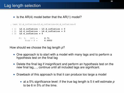
• Is the AR(4) model better that the AR(1) model?
Thursday April 17 10:26:49 2014 Page 1
___ ____ ____ ____ ____(R) /__ / ____/ / ____/ ___/ / /___/ / /___/ Statistics/Data Analysis
1 . test L2.d_inflation=L3.d_inflation=L4.d_inflation=0
( 1) L2.d_inflation - L3.d_inflation = 0 ( 2) L2.d_inflation - L4.d_inflation = 0 ( 3) L2.d_inflation = 0
F( 3, 167) = 6.71 Prob > F = 0.0003
How should we choose the lag length p?
• One approach is to start with a model with many lags and to perform ahypothesis test on the final lag
• Delete the final lag if insignificant and perform an hypothesis test on thenew final lag,..., continue until all included lags are significant.
• Drawback of this approach is that it can produce too large a model
• at a 5% significance level: if the true lag length is 5 it will estimate pto be 6 in 5% of the time.
21
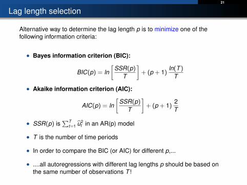
Lag length selection
Alternative way to determine the lag length p is to minimize one of thefollowing information criteria:
• Bayes information criterion (BIC):
BIC(p) = ln[
SSR(p)T
]+ (p + 1)
ln(T )
T
• Akaike information criterion (AIC):
AIC(p) = ln[
SSR(p)T
]+ (p + 1)
2T
• SSR(p) is∑T
t=1 u2t in an AR(p) model
• T is the number of time periods
• In order to compare the BIC (or AIC) for different p,...
• ....all autoregressions with different lag lengths p should be based onthe same number of observations T !

22
Lag length selection
The BIC and AIC both consist of two terms:
• 1st term ln[
SSR(p)T
]: always decreasing in p
• larger p, better fit
• 2nd term (p + 1) ln(T )T (BIC) or (p + 1) 2
T (AIC): always increasing in p.
• This term is a “penalty” for estimating more parameters – and thusincreasing the RMSFE.
AIC estimates more lags (larger p) than the BIC for T > 7.4,
• the penalty term is smaller for AIC than BIC
In large samples the AIC overestimates p, it is inconsistent.

23
Lag length selection
Thursday April 17 11:19:16 2014 Page 1
___ ____ ____ ____ ____(R) /__ / ____/ / ____/ ___/ / /___/ / /___/ Statistics/Data Analysis
1 . regress d_inflation L1.d_inflation if tin(1962q1,2004q4), r
Linear regression Number of obs = 172 F( 1, 170) = 6.08 Prob > F = 0.0146 R-squared = 0.0564 Root MSE = 1.664
Robust d_inflation Coef. Std. Err. t P>|t| [95% Conf. Interval]
d_inflation L1. -.2380471 .0965017 -2.47 0.015 -.4285431 -.047551 _cons .0171008 .1268849 0.13 0.893 -.2333721 .2675736
2 . gen BIC_1=ln(e(rss)/e(N))+e(rank)*(ln(e(N))/e(N)) if tin(1962q1,2004q4)(21 missing values generated)
3 . gen AIC_1=ln(e(rss)/e(N))+e(rank)*(2/e(N)) if tin(1962q1,2004q4)(21 missing values generated)
4 . sum BIC_1 AIC_1
Variable Obs Mean Std. Dev. Min Max
BIC_1 172 1.066562 0 1.066562 1.066562 AIC_1 172 1.029963 0 1.029963 1.029963

24
Lag length selection
BIC AIC
Thursday April 17 11:22:18 2014 Page 1
___ ____ ____ ____ ____(R) /__ / ____/ / ____/ ___/ / /___/ / /___/ Statistics/Data Analysis
1 . sum BIC*
Variable Obs Mean Std. Dev. Min Max
BIC_0 172 1.094665 0 1.094665 1.094665 BIC_1 172 1.066562 0 1.066562 1.066562 BIC_2 172 .9549263 0 .9549263 .9549263 BIC_3 172 .9574141 1.11e-16 .9574141 .9574141 BIC_4 172 .9864399 0 .9864399 .9864399
Thursday April 17 11:23:04 2014 Page 1
___ ____ ____ ____ ____(R) /__ / ____/ / ____/ ___/ / /___/ / /___/ Statistics/Data Analysis
1 . sum AIC*
Variable Obs Mean Std. Dev. Min Max
AIC_0 172 1.076366 0 1.076366 1.076366 AIC_1 172 1.029963 0 1.029963 1.029963 AIC_2 172 .9000281 0 .9000281 .9000281 AIC_3 172 .8842165 0 .8842165 .8842165 AIC_4 172 .894943 0 .894943 .894943
• Optimal lag length according to BIC: p = 2
• Optimal lag length according to AIC: p = 3

25
Autoregressive Distributed Lag Model (ADL(p,q))
• Economic theory often suggests other variables that could help toforecast the variable of interest.
• When we add other variables and their lags the result is an
autoregressive distributed lag model ADL(p,q)
Yt = β0 + β1Yt−1 + ...+ βpYt−p + δ1Xt−1 + ...+ δqXt−q + ut
• p is the number of lags of the dependent variable
• q is the number of lags (distributed lags) of the additional predictor X

26
Autoregressive Distributed Lag Model (ADL(p,q))
• When predicting future changes in inflation economic theory suggeststhat lagged values of the unemployment rate might be a good predictor
• Short-run Philips curve: negative short run relation betweenunemployment and inflation
• According to Bays Information Criteria we should include 2 lags of thedependent variable
• In addition we include 2 lags of the unemployment rate
• This gives an ADL(2,2) model

27
Autoregressive Distributed Lag Model (ADL(p,q))
Thursday April 17 12:05:17 2014 Page 1
___ ____ ____ ____ ____(R) /__ / ____/ / ____/ ___/ / /___/ / /___/ Statistics/Data Analysis
> regress d_inflation L1.d_inflation L2.d_inflation L1.unemployment L2.unemployment if > tin(1962q1,2004q4), r
Linear regression Number of obs = 172 F( 4, 167) = 15.41 Prob > F = 0.0000 R-squared = 0.3514 Root MSE = 1.3918
Robust d_inflation Coef. Std. Err. t P>|t| [95% Conf. Interval]
d_inflation L1. -.4685035 .0771115 -6.08 0.000 -.6207425 -.3162645 L2. -.4251441 .0821394 -5.18 0.000 -.5873096 -.2629787 unemployment_rate L1. -2.243865 .4020402 -5.58 0.000 -3.037602 -1.450129 L2. 2.044221 .3875693 5.27 0.000 1.279054 2.809388 _cons 1.193032 .4344711 2.75 0.007 .3352683 2.050796
1 . dis "Adjusted Rsquared = " _result(8)Adjusted Rsquared = .3358903
• Adjusted R2 is higher and the RMSE is lower in ADL(2,2) than in AR(4)
• Forecast error = 4inf2005q1 − 4inf 2005q1|2004q4 = −1.14− (0.38) = −1.52

28
Granger “causality” test
• Do the included lags of unemployment have useful predictive contentconditional on the included lags of the change in inflation?
• The claim that a variable has no predictive content corresponds to thenull hypothesis that the coefficients on all lags of the variable are zero.
• The F-statistic of this test is called the Granger causality statistic.
• If the null hypothesis is rejected the variable X is said to Granger-causethe dependent variable Y .
• This does not mean that we have estimated the causal effect of X on Y!!
• It means that X is a useful predictor of Y (Granger predictability wouldbe a better term).

29
Granger “causality” test
The Granger causality test in the ADL(2,2) model:
Tuesday April 22 13:40:48 2014 Page 1
___ ____ ____ ____ ____(R) /__ / ____/ / ____/ ___/ / /___/ / /___/ Statistics/Data Analysis
1 . 2 . regress d_inflation L1.d_inflation L2.d_inflation L1.unemployment L2.unemployment if
> tin(1962q1,2004q4), r noheader
Robust d_inflation Coef. Std. Err. t P>|t| [95% Conf. Interval]
d_inflation L1. -.4685035 .0771115 -6.08 0.000 -.6207425 -.3162645 L2. -.4251441 .0821394 -5.18 0.000 -.5873096 -.2629787 unemployment_rate L1. -2.243865 .4020402 -5.58 0.000 -3.037602 -1.450129 L2. 2.044221 .3875693 5.27 0.000 1.279054 2.809388 _cons 1.193032 .4344711 2.75 0.007 .3352683 2.050796
3 . test L1.unemployment=L2.unemployment=0
( 1) L.unemployment_rate - L2.unemployment_rate = 0 ( 2) L.unemployment_rate = 0
F( 2, 167) = 16.13 Prob > F = 0.0000
• Null hypothesis that coefficients on the 2 lags of unemployment are zerois rejected at a 1% level.
• Unemployment is a useful predictor for the change in the inflation rate.

30
Nonstationarity: trends
• A time series Yt is stationary if its probability distribution does notchange over time
• If a time series has a trend, it is nonstationary
• A trend is a persistent long-term movement of a variable over time.
• We consider two types of trends
Deterministic trend: Yt = β0 + λt + u1
• series is a nonrandom function of time
Stochastic trend: Yt = β0 + Yt−1 + u1
• series is a random function of time

31
Nonstationarity: trends
Deterministic trend Stochastic trend
20
40
60
80
100
Y
0 20 40 60 80 100Time
20
40
60
80
100
Y
0 20 40 60 80 100Time

32
Random walk model
• Simplest model of a variable with a stochastic trend is the random walk
Yt = Yt−1 + ut where ut is i .i.d .
• The value of the series tomorrow is its value today plus an unpredictablechange.
• An extension of the random walk model is the random walk with drift
Yt = β0 + Yt−1 + ut where ut is i .i.d .
• β0 is the “drift” of the random walk, if β0 is positive Yt increases onaverage.
• A random walk is nonstationary: the distribution is not constant over time
• The variance of a random walk increases over time:
Var (Yt) = Var (Yt−t) + Var (ut)

33
Stochastic trends, autoregressive models and a unit root
• The random walk model is a special case of an AR(1) model with β1 = 1
• If Yt follows and AR(1) with |β1| < 1 (and ut is stationary), Yt isstationary
• If Yt follows and AR(p) model
Yt = β0 + β1Yt−1 + β2Yt−2 + ...+ βpYt−p + ut
Yt is stationary if its roots z are all greater than 1 in absolute value.
• the roots are the values of z that satisfy
1− β1z − β2z2 − ...− βpzp = 0
• In the special case of an AR(1): 1− β1z = 0 gives z = 1β1
which isbigger than |1| if |β1| < 1

34
Detecting stochastic trends: Dickey-Fuller test in AR(1) model
• Trends can be detected by informal and formal methods
• Informal: inspect the time series plot
• Formal: Perform the Dickey-Fuller test to test for a stochastictrend.
• Dickey-Fuller test in an AR(1) model:
H0 : β1 = 1 vs H1 : β1 < 1 in Yt = β0 + β1Yt−1 + ut
• Test can be performed by subtracting Yt−1 from both sides of theequation and estimate
4Yt = β0 + δYt−1 + εt
• We can now test
H0 : δ = β1 − 1 = 0 vs H1 : δ < 0

35
Does U.S. inflation have a stochastic trend?
• DF test for a unit root in U.S. inflation (Note: we test for a stochastictrend in inflationt and not in 4inflationt )
Tuesday April 22 15:13:32 2014 Page 1
___ ____ ____ ____ ____(R) /__ / ____/ / ____/ ___/ / /___/ / /___/ Statistics/Data Analysis
1 . regress d_inflation L1.inflation if tin(1962q1,2004q4), noheader
d_inflation Coef. Std. Err. t P>|t| [95% Conf. Interval]
inflation L1. -.1643553 .0415311 -3.96 0.000 -.2463383 -.0823722 _cons .7219345 .217599 3.32 0.001 .2923904 1.151479
• Under H0 ,Yt is nonstationary and the DF-statistic has a nonnormaldistribution, we therefore use the following critical values
Copyright © 2011 Pearson Addison-Wesley. All rights reserved. 14-88
Table of DF Critical Values
(a) ∆Yt = β0 + δYt–1 + ut (intercept only)(b) ∆Yt = β0 + μt + δYt–1 + ut (intercept and time trend)
Reject if the DF t-statistic (the t-statistic testing δ = 0) is less than the specified critical value. This is a 1-sided test of the null hypothesis of a unit root (random walk trend) vs. the alternative that the autoregression is stationary.
• DF = −3.96 this is more negative than -2.86 so we reject the nullhypothesis of a stochastic trend at a 5% significance level.

36
Detecting stochastic trends: Dickey-Fuller test in AR(p) model
• Often an AR(1) model does not capture all the serial correlation in Yt
and we should include more lags & estimate an AR(p) model.
• We can test for a stochastic trend in an AR(p) model by augmenting theDF-regression by lags of 4Yt .
• The Augmented Dickey-Fuller test:
H0 : δ = 0 vs H1 : δ < 0
in the regression
4Yt = β0 + δYt−1 + γ14Yt−1 + γ24Yt−2 + ...+ γp4Yt−p + ut
• Note: The DF-statistic should be computed using homoskedasticity-only(nonrobust) standard errors (see footnote 3 in S&W CH14)

37
Does U.S. inflation have a stochastic trend?
• DF test for a unit root in U.S. inflation – using p = 4 lags (AR(4)-model)
Tuesday April 22 15:41:26 2014 Page 1
___ ____ ____ ____ ____(R) /__ / ____/ / ____/ ___/ / /___/ / /___/ Statistics/Data Analysis
1 . regress d_inflation L1.inflation L1.d_inflation L2.d_inflation L3.d_inflation L4.d_in> flation if tin(1962q1,2004q4), noheader
d_inflation Coef. Std. Err. t P>|t| [95% Conf. Interval]
inflation L1. -.1134169 .0422344 -2.69 0.008 -.1968029 -.030031 d_inflation L1. -.1864426 .0805144 -2.32 0.022 -.3454068 -.0274783 L2. -.2563879 .081463 -3.15 0.002 -.4172251 -.0955507 L3. .1990491 .0793514 2.51 0.013 .0423811 .3557171 L4. .0099994 .0779921 0.13 0.898 -.1439849 .1639837 _cons .5068158 .2141807 2.37 0.019 .0839466 .9296851
• DF = −2.69 this is less negative than -2.86 so we do not reject the nullhypothesis of a stochastic trend at a 5% significance level.

38
Does U.S. inflation have a stochastic trend?
• Instead of testing the null hypothesis of a stochastic trend against thealternative hypothesis of no trend....
• ...the alternative hypothesis can be that Yt is stationary around adeterministic trend.
• The Dickey-Fuller regression then includes a deterministic trend
4Yt = β0 + αt + δYt−1 + γ14Yt−1 + γ24Yt−2 + ...+ γp4Yt−p + ut
• And we have to use the critical values in the second row:
Copyright © 2011 Pearson Addison-Wesley. All rights reserved. 14-88
Table of DF Critical Values
(a) ∆Yt = β0 + δYt–1 + ut (intercept only)(b) ∆Yt = β0 + μt + δYt–1 + ut (intercept and time trend)
Reject if the DF t-statistic (the t-statistic testing δ = 0) is less than the specified critical value. This is a 1-sided test of the null hypothesis of a unit root (random walk trend) vs. the alternative that the autoregression is stationary.

39
Avoiding problems caused by stochastic trends
• Best way to deal with a trend is to transform the series such that it doesnot have a trend.
• If the series Yt has a stochastic trend, then the first difference of theseries 4Yt does not have a stochastic trend.
• For example if Yt follows a random walk with drift
Yt = β0 + Yt−1 + ut
the first difference is stationary
4Yt = β0 + ut
• On slide 37 we saw that we did not reject the null hypothesis of astochastic trend in inflationt .
• This is the reason that in the beginning of the lecture we estimated AR’swith 4inflationt .

40
0
5
10
15
Infla
tion
(%)
1957q1 1969q1 1981q1 1993q1 2005q1
time
-6
-4
-2
0
2
4
Cha
nge
in in
flatio
n
1957q1 1969q1 1981q1 1993q1 2005q1
time

41
Good luck with the exam!(Don’t forget to bring the book and a calculator!)