efficient optimization of memory accesses in …vs3/pdf/rajbarik_thesis.pdfabstract efficient...
TRANSCRIPT
RICE UNIVERSITY
Efficient Optimization of Memory Accesses in
Parallel Programs
by
Rajkishore Barik
A Thesis Submitted
in Partial Fulfillment of the
Requirements for the Degree
Doctor of Philosophy
Approved, Thesis Committee:
Vivek Sarkar, ChairE.D. Butcher Professor of ComputerScience
Keith CooperL. John and Ann H. Doerr Professor ofComputer Science
Timothy HarveyResearch ScientistDept. of Computer Science
Lin ZhongAssistant ProfessorDept. of Electrical Engineering &Computer Science
Houston, Texas
October, 2009
ABSTRACT
Efficient Optimization of Memory Accesses in Parallel
Programs
by
Rajkishore Barik
The power, frequency, and memory wall problems have caused a major shift in
mainstream computing by introducing processors that contain multiple low power
cores. As multi-core processors are becoming ubiquitous, software trends in both
parallel programming languages and dynamic compilation have added new challenges
to program compilation for multi-core processors. This thesis proposes a combination
of high-level and low-level compiler optimizations to address these challenges.
The high-level optimizations introduced in this thesis include new approaches to
May-Happen-in-Parallel analysis and Side-Effect analysis for parallel programs and
a novel parallelism-aware Scalar Replacement for Load Elimination transformation.
A new Isolation Consistency (IC) memory model is described that permits several
scalar replacement transformation opportunities compared to many existing memory
models.
The low-level optimizations include a novel approach to register allocation that
retains the compile time and space efficiency of Linear Scan, while delivering runtime
performance superior to both Linear Scan and Graph Coloring. The allocation phase
is modeled as an optimization problem on a Bipartite Liveness Graph (BLG) data
structure. The assignment phase focuses on reducing the number of spill instructions
by using register-to-register move and exchange instructions wherever possible.
Experimental evaluations of our scalar replacement for load elimination transfor-
mation in the Jikes RVM dynamic compiler show decreases in dynamic counts for
getfield operations of up to 99.99%, and performance improvements of up to 1.76×on 1 core, and 1.39× on 16 cores, when compared with the load elimination algorithm
available in Jikes RVM. A prototype implementation of our BLG register allocator in
Jikes RVM demonstrates runtime performance improvements of up to 3.52× relative
to Linear Scan on an x86 processor. When compared to Graph Coloring register
allocator in the GCC compiler framework, our allocator resulted in an execution time
improvement of up to 5.8%, with an average improvement of 2.3% on a POWER5
processor.
With the experimental evaluations combined with the foundations presented in
this thesis, we believe that the proposed high-level and low-level optimizations are
useful in addressing some of the new challenges emerging in the optimization of
parallel programs for multi-core architectures.
Acknowledgments
I would like to express my appreciation to my thesis committee, especially to my
adviser, Prof. Vivek Sarkar, for his patient guidance and support. He is always full
of energy and enthusiasm for attacking research problems and possesses one of the
sharper brains. The door to his office was always open whenever I ran into a trouble
spot in both academically and personally. And during the most difficult times when
writing this thesis, he gave me the moral support and the freedom I needed to move
on. It was an honor to work with him. I owe my deepest gratitude to my thesis
co-chair Prof. Keith D. Cooper for his technical advice during the course work of
COMP 512 that went onto play an important role in my thesis work. I am grateful to
my thesis co-chair Dr. Timothy J. Harvey for his guidance on register allocation and
his useful suggestions and advice that significantly helped improving the presentation
of this thesis. There are several people at Rice University that helped me during
my graduate career including Prof. Lin Zhong, David Peixotto, Jisheng Zhao, Jun
Shirako, Yi Guo, Raghavan Raman, and Prof. John Mellor-Crummey.
I had the privilege to work under Prof. Thomas Gross, my advisor at ETH, Zurich.
His guidance and support has been invaluable during my early graduate school days.
I also recognize the enormous amount of help provided by Dr. Christoph von Praun
on clarifying my innumerable doubts on ERCO infrastructure at ETH.
This thesis would not have been possible without support from my managers at
IBM who allowed me to pursue Ph.D. while being a full-time employee. I would
like to thank my managers at IBM including Dr. Ravi Kothari, Dr. Sugata Ghosal,
Dr. R. K. Shyamasundar, Dr. Calin Cascaval, Dr. Rahul Garg, and Dr. Vijay
Saraswat. It has been enjoyable experience working with them. I would like to thank

v
all members of the X10 team at IBM for valuable discussions and feedback related
to this thesis work, especially Igor Peshansky for discussion of the semantics of Java
final variables. I am thankful to all X10 team members for their contributions to the
X10 software used in this thesis. I gratefully acknowledge the support from an IBM
Open Collaborative Faculty Award. This work was supported in part by the National
Science Foundation under the HECURA program, award number CCF-0833166.
I would like to acknowledge my collaborators Shivali Agarwal and Prof. R. K.
Shyamasundar from TIFR. The work on May-Happens-in-Parallel (MHP) analysis in
Chapter 3 was done with their collaboration. I would also like to thank IBM Summer
intern, Puneet Goyal, for his work on bitwidth-aware packing that led to our work in
Chapter 7.
Finally, I gratefully acknowledge my family’s love and encouragement. My beloved
wife, Meena, has been a constant source of inspiration during the rough times of
graduate life. Her patience, love and encouragement have upheld me, particularly
in those many days in which I spent more time with computer than with her. I
dedicate my thesis to her. I owe my deepest gratitude to my IBM colleague and close
friend, Rema Ananthanarayan, for motivating me to come to Rice and for helping me
personally.
Contents
Abstract ii
Acknowledgments iv
List of Illustrations xi
List of Tables xv
1 Introduction 1
1.1 Research Contributions . . . . . . . . . . . . . . . . . . . . . . . . . . 4
1.2 Thesis Organization . . . . . . . . . . . . . . . . . . . . . . . . . . . . 6
2 Background 7
2.1 Basics of a Compiler . . . . . . . . . . . . . . . . . . . . . . . . . . . 7
2.2 The HJ Parallel Programming Language . . . . . . . . . . . . . . . . 11
2.2.1 Single Place HJ Language Constructs . . . . . . . . . . . . . . 12
2.2.2 Multi-Place Programming in HJ . . . . . . . . . . . . . . . . . 16
2.2.2.1 Remote Asyncs . . . . . . . . . . . . . . . . . . . . . 18
2.3 Code Optimization Framework . . . . . . . . . . . . . . . . . . . . . . 19
2.4 May-Happen-in-Parallel (MHP) Analysis . . . . . . . . . . . . . . . . 21
2.4.1 MHP Analysis for Java Programs . . . . . . . . . . . . . . . . 23
2.5 Side-Effect Analysis . . . . . . . . . . . . . . . . . . . . . . . . . . . . 27
2.6 Scalar Replacement Transformation for Load Elimination . . . . . . . 31
2.6.1 Unified Modeling of Arrays and Objects . . . . . . . . . . . . 33
2.6.2 Extended Array SSA form . . . . . . . . . . . . . . . . . . . . 34
2.6.3 Load Elimination Algorithm . . . . . . . . . . . . . . . . . . . 34
2.7 Register Allocation . . . . . . . . . . . . . . . . . . . . . . . . . . . . 36
vii
2.7.1 Terminology . . . . . . . . . . . . . . . . . . . . . . . . . . . . 37
2.7.1.1 Liveness, Live-ranges and Interference Graph . . . . 37
2.7.1.2 Spilling . . . . . . . . . . . . . . . . . . . . . . . . . 38
2.7.1.3 Coalescing . . . . . . . . . . . . . . . . . . . . . . . . 38
2.7.1.4 Live-range splitting . . . . . . . . . . . . . . . . . . . 39
2.7.1.5 Architectural Considerations . . . . . . . . . . . . . 39
2.7.2 Register Allocation Techniques . . . . . . . . . . . . . . . . . 40
2.7.2.1 Graph Coloring Register Allocation . . . . . . . . . . 40
2.7.2.2 Linear Scan Register Allocation . . . . . . . . . . . . 43
2.7.2.3 SSA-based Register Allocation . . . . . . . . . . . . 50
2.8 Bitwidth-aware Register Allocation . . . . . . . . . . . . . . . . . . . 52
2.8.1 Bitwidth Analysis . . . . . . . . . . . . . . . . . . . . . . . . . 55
2.8.2 Variable Packing . . . . . . . . . . . . . . . . . . . . . . . . . 56
2.8.3 Move Insertion . . . . . . . . . . . . . . . . . . . . . . . . . . 58
2.8.4 Register Allocation . . . . . . . . . . . . . . . . . . . . . . . . 59
3 May-Happen-in-Parallel (MHP) Analysis 60
3.1 Introduction . . . . . . . . . . . . . . . . . . . . . . . . . . . . . . . . 60
3.2 Steps for MHP analysis of HJ programs . . . . . . . . . . . . . . . . . 61
3.3 Program Structure Tree (PST) Representation . . . . . . . . . . . . . 62
3.3.1 Example . . . . . . . . . . . . . . . . . . . . . . . . . . . . . . 63
3.4 Never-Execute-in-Parallel Analysis . . . . . . . . . . . . . . . . . . . 65
3.4.1 Comparison with MHP Analysis of Java programs . . . . . . . 67
3.4.2 Complexity . . . . . . . . . . . . . . . . . . . . . . . . . . . . 74
3.4.3 Example . . . . . . . . . . . . . . . . . . . . . . . . . . . . . . 74
3.5 Place Equivalence Analysis . . . . . . . . . . . . . . . . . . . . . . . . 76
3.5.1 Complexity . . . . . . . . . . . . . . . . . . . . . . . . . . . . 81
3.5.2 Example . . . . . . . . . . . . . . . . . . . . . . . . . . . . . . 81

viii
3.6 MHP Analysis using Isolated Sections . . . . . . . . . . . . . . . . . . 81
3.6.1 Complexity . . . . . . . . . . . . . . . . . . . . . . . . . . . . 83
3.6.2 Example . . . . . . . . . . . . . . . . . . . . . . . . . . . . . . 83
3.7 Summary . . . . . . . . . . . . . . . . . . . . . . . . . . . . . . . . . 84
4 Side-Effect Analysis for Parallel Programs 85
4.1 Side-Effect Analysis of Method Calls . . . . . . . . . . . . . . . . . . 86
4.1.1 Heap Array Representation . . . . . . . . . . . . . . . . . . . 88
4.1.2 Method Level Side-effect . . . . . . . . . . . . . . . . . . . . . 88
4.1.3 Complexity . . . . . . . . . . . . . . . . . . . . . . . . . . . . 91
4.1.4 Discussion . . . . . . . . . . . . . . . . . . . . . . . . . . . . . 92
4.2 Extended Side-effect Analysis for Parallel Constructs . . . . . . . . . 92
4.2.1 Side-Effects for Finish Scopes . . . . . . . . . . . . . . . . . . 94
4.2.2 Side-Effects for Methods with Escaping Asyncs . . . . . . . . 95
4.2.3 Side-Effects for Isolated Blocks . . . . . . . . . . . . . . . . . 96
4.3 Parallelism-aware Side-Effect Analysis Algorithm . . . . . . . . . . . 98
4.3.1 Discussion . . . . . . . . . . . . . . . . . . . . . . . . . . . . . 101
4.4 Summary . . . . . . . . . . . . . . . . . . . . . . . . . . . . . . . . . 103
5 Isolation Consistency Memory Model and its Impact on
Scalar Replacement 105
5.1 Program Transformation and Memory Model . . . . . . . . . . . . . . 105
5.2 Isolation Consistency Memory Model . . . . . . . . . . . . . . . . . . 108
5.2.1 Abstraction . . . . . . . . . . . . . . . . . . . . . . . . . . . . 109
5.2.2 State-Update rules for L . . . . . . . . . . . . . . . . . . . . . 110
5.2.3 State Observability for L . . . . . . . . . . . . . . . . . . . . . 112
5.2.4 Example Scenarios . . . . . . . . . . . . . . . . . . . . . . . . 113
5.3 Scalar Replacement for Load Elimination . . . . . . . . . . . . . . . . 115
ix
5.3.1 Example . . . . . . . . . . . . . . . . . . . . . . . . . . . . . . 117
5.4 Summary . . . . . . . . . . . . . . . . . . . . . . . . . . . . . . . . . 117
6 Space-Efficient Register Allocation 120
6.1 Notions Revisited . . . . . . . . . . . . . . . . . . . . . . . . . . . . . 121
6.2 Example . . . . . . . . . . . . . . . . . . . . . . . . . . . . . . . . . . 123
6.3 Overall Approach . . . . . . . . . . . . . . . . . . . . . . . . . . . . . 126
6.4 Allocation using Bipartite Liveness Graphs . . . . . . . . . . . . . . . 129
6.4.1 Eager Heuristic . . . . . . . . . . . . . . . . . . . . . . . . . . 132
6.5 Assignment using Register Moves and Exchanges . . . . . . . . . . . 134
6.5.1 Spill-Free Assignment . . . . . . . . . . . . . . . . . . . . . . . 134
6.5.2 Example . . . . . . . . . . . . . . . . . . . . . . . . . . . . . . 138
6.5.3 Assignment with Move Coalescing and Register Moves . . . . 140
6.6 Allocation and Assignment with Register Classes . . . . . . . . . . . 143
6.6.1 Constrained Allocation using BLG . . . . . . . . . . . . . . . 145
6.6.2 Constrained Assignment . . . . . . . . . . . . . . . . . . . . . 145
6.7 Extended Linear Scan (ELS) . . . . . . . . . . . . . . . . . . . . . . . 149
6.8 Summary . . . . . . . . . . . . . . . . . . . . . . . . . . . . . . . . . 150
7 Bitwidth-aware Register Allocation 152
7.1 Overall Bitwidth-aware register allocation . . . . . . . . . . . . . . . 153
7.2 Limit Study . . . . . . . . . . . . . . . . . . . . . . . . . . . . . . . . 153
7.3 Enhanced Bitwidth Analysis . . . . . . . . . . . . . . . . . . . . . . . 156
7.4 Enhanced Packing . . . . . . . . . . . . . . . . . . . . . . . . . . . . 160
7.4.1 Improved EMIW estimates . . . . . . . . . . . . . . . . . . . . 164
7.5 Summary . . . . . . . . . . . . . . . . . . . . . . . . . . . . . . . . . 164
8 Performance Results 166
8.1 Side-Effect Analysis and Load Elimination . . . . . . . . . . . . . . . 166
x
8.1.1 Experimental setup . . . . . . . . . . . . . . . . . . . . . . . . 166
8.1.2 Experimental results . . . . . . . . . . . . . . . . . . . . . . . 168
8.2 Space-Efficient Register Allocation . . . . . . . . . . . . . . . . . . . 176
8.2.1 GCC Evaluation . . . . . . . . . . . . . . . . . . . . . . . . . 176
8.2.1.1 Experimental setup . . . . . . . . . . . . . . . . . . . 176
8.2.1.2 Experimental results . . . . . . . . . . . . . . . . . . 178
8.2.2 Jikes RVM evaluation . . . . . . . . . . . . . . . . . . . . . . 179
8.2.2.1 Experimental setup . . . . . . . . . . . . . . . . . . . 179
8.2.2.2 Experimental results . . . . . . . . . . . . . . . . . . 180
8.3 Bitwidth-Aware Register Allocation . . . . . . . . . . . . . . . . . . . 182
8.3.1 Experimental setup . . . . . . . . . . . . . . . . . . . . . . . . 182
8.3.2 Experimental results . . . . . . . . . . . . . . . . . . . . . . . 183
8.4 Summary . . . . . . . . . . . . . . . . . . . . . . . . . . . . . . . . . 185
9 Conclusions and Future Work 187
9.1 Future Work . . . . . . . . . . . . . . . . . . . . . . . . . . . . . . . . 189
Illustrations
2.1 Example control flow graph (CFG) . . . . . . . . . . . . . . . . . . . 8
2.2 HJ’s Multi-Place Execution Model . . . . . . . . . . . . . . . . . . . . 17
2.3 Static and Dynamic Optimization Framework . . . . . . . . . . . . . 19
2.4 CFG structures for depicting various side-effects . . . . . . . . . . . . 28
2.5 Termination of Side-effect analysis . . . . . . . . . . . . . . . . . . . . 31
2.6 Examples of scalar replacement for load elimination transformation . 32
2.7 Load elimination algorithm . . . . . . . . . . . . . . . . . . . . . . . 35
2.8 Chaitin’s Register Allocator . . . . . . . . . . . . . . . . . . . . . . . 42
2.9 Linear Scan register allocation algorithm . . . . . . . . . . . . . . . . 47
2.10 Demonstration of intervals in Linear Scan register allocation . . . . . 48
2.11 Examples of chordal and non-chordal graphs . . . . . . . . . . . . . . 51
2.12 SSA-based register allocation . . . . . . . . . . . . . . . . . . . . . . 52
2.13 Example code fragment demonstrating bitwidth-aware register
allocation . . . . . . . . . . . . . . . . . . . . . . . . . . . . . . . . . 54
2.14 Bitwidth-aware register allocation framework . . . . . . . . . . . . . . 54
2.15 Scenarios for precise variable packing using MIW . . . . . . . . . . . 57
2.16 Scenario for variable packing using EMIW . . . . . . . . . . . . . . . 58
3.1 Example HJ program to demonstrate the computation of MHP(S1, S2). 64
3.2 PST for example program in Figure 3.1 . . . . . . . . . . . . . . . . . 64
3.3 Algorithm for computing Never-Execute-in-Parallel (NEP) relations . 66
3.4 Java example program to illustrate MHP algorithm . . . . . . . . . . 67
xii
3.5 HJ example program to illustrate NEP algorithm . . . . . . . . . . . 68
3.6 PST for example program in Fig 3.5 . . . . . . . . . . . . . . . . . . 68
3.7 Java code example that demonstrates that NEP(S1, S2) is not just a
binary relation . . . . . . . . . . . . . . . . . . . . . . . . . . . . . . 70
3.8 HJ code example that demonstrates that NEP(S1, S2) is not just a
binary relation . . . . . . . . . . . . . . . . . . . . . . . . . . . . . . 71
3.9 Algorithm for computing refined Never-Execute-in-Parallel (NEP)
relations . . . . . . . . . . . . . . . . . . . . . . . . . . . . . . . . . . 73
3.10 (BLOCK, ∗) distribution of array A[p, p] that uses p places . . . . . . . 79
3.11 Algorithm for computing Place Equivalence (PE) relations . . . . . . 80
3.12 Algorithm for computing May-Happen-in-Parallel (MHP) relation
using place equivalence and isolated sections in HJ . . . . . . . . . . . 82
4.1 Side-effect analysis enables more opportunities for scalar replacement 87
4.2 Lattice for heap array GMOD and GREF sets . . . . . . . . . . . . . 89
4.3 Fast Side-effect analysis for a given method m . . . . . . . . . . . . . 90
4.4 Side-effect analysis can improve the analysis by reasoning about
object references . . . . . . . . . . . . . . . . . . . . . . . . . . . . . 92
4.5 Example HJ program for side-effect analysis in the presence of
parallel constructs. . . . . . . . . . . . . . . . . . . . . . . . . . . . . 93
4.6 Call graph for example program in Figure 4.5 . . . . . . . . . . . . . 94
4.7 ParallelSideEffectAnalysis(m): Side-effect analysis in the
presence of HJ parallel constructs for method m . . . . . . . . . . . . 99
4.8 Additional function to handle method calls for
ParallelSideEffectAnalysis(m) . . . . . . . . . . . . . . . . . . . 100
4.9 Additional functions to handle async calls and normal method calls
for ParallelSideEffectAnalysis(m) . . . . . . . . . . . . . . . . . 102
4.10 Improving the precision of global isolated side-effects. . . . . . . . . . 104
xiii
5.1 Example program illustrating violation of Sequential Consistency due
to reordering within a thread . . . . . . . . . . . . . . . . . . . . . . 107
5.2 Four parallel code fragments that demonstrate scalar replacement for
load elimination opportunities in the presence of parallel constructs. . 114
5.3 Parallelism-aware scalar replacement for load elimination
transformation . . . . . . . . . . . . . . . . . . . . . . . . . . . . . . 116
5.4 Example HJ program for parallelism-aware scalar replacement
transformation . . . . . . . . . . . . . . . . . . . . . . . . . . . . . . 118
5.5 Transformed program after scalar replacement for program shown in
Figure 5.4 . . . . . . . . . . . . . . . . . . . . . . . . . . . . . . . . . 119
6.1 Example program for illustrating space-efficient register allocation . . 123
6.2 Example program for illustrating Space-efficient register allocation . . 127
6.3 Overall Space Efficient Register Allocator using BLG. . . . . . . . . . 127
6.4 SSA based Register Allocation. This figure is adapted from [22]. . . . 128
6.5 Greedy heuristic to perform allocation using max-min strategy. . . . . 131
6.6 Eager heuristic to perform allocation . . . . . . . . . . . . . . . . . . 133
6.7 Assignment using register move and exchange instructions . . . . . . 135
6.8 Algorithm to insert register move and exchange instructions on
control flow edges . . . . . . . . . . . . . . . . . . . . . . . . . . . . . 137
6.9 Anti-dependence graph (D) for the example program in Figure 6.1 . . 138
6.10 Greedy heuristic to choose a physical register for a basic interval that
maximizes copy removal. . . . . . . . . . . . . . . . . . . . . . . . . . 142
6.11 Register classes in the Intel x86 architecture . . . . . . . . . . . . . . 143
6.12 Example program demonstrating problems associated with register
assignment using register classes . . . . . . . . . . . . . . . . . . . . . 143
6.13 Example demonstrating problems in coalescing due to register classes 144
6.14 Heuristic o perform assignment in the presence of register classes . . . 147
xiv
6.15 Heuristic to choose a physical register that maximizes copy removal. . 148
6.16 Overview of Extended Linear Scan algorithm (ELS) with
all-or-nothing approach . . . . . . . . . . . . . . . . . . . . . . . . . . 151
7.1 Overall Bitwidth-aware register allocation framework. . . . . . . . . . 152
7.2 GCC modification for Limit Study . . . . . . . . . . . . . . . . . . . 154
7.3 Recurrence analysis for bitwidth analysis . . . . . . . . . . . . . . . . 158
7.4 Code fragment from BITWISE adpcm benchmark. . . . . . . . . . . . 159
7.5 Code fragment from BITWISE bubblesort benchmark. . . . . . . . 159
7.6 Example program for demonstrating imprecision in Tallam-Gupta
packing . . . . . . . . . . . . . . . . . . . . . . . . . . . . . . . . . . 161
7.7 Interference Graph for the example program shown in Figure 7.6 . . . 161
7.8 Bitwidth aware register allocation in a graph coloring scenario. . . . . 163
8.1 Performance improvement using the scalar replacement algorithm
presented in Figure 5.3 . . . . . . . . . . . . . . . . . . . . . . . . . . 174
8.2 Scaling of JGF Section 3 MolDyn Size B benchmark . . . . . . . . . . 175
8.3 Scaling of NPB CG Size A benchmark . . . . . . . . . . . . . . . . . 175
8.4 SPEC rates for Graph Coloring and ELS register Allocator described
in Section 6.7. . . . . . . . . . . . . . . . . . . . . . . . . . . . . . . . 177
8.5 Speedup of BLG with register classes relative to LS . . . . . . . . . . 181
8.6 GCC modification for register allocation . . . . . . . . . . . . . . . . 184
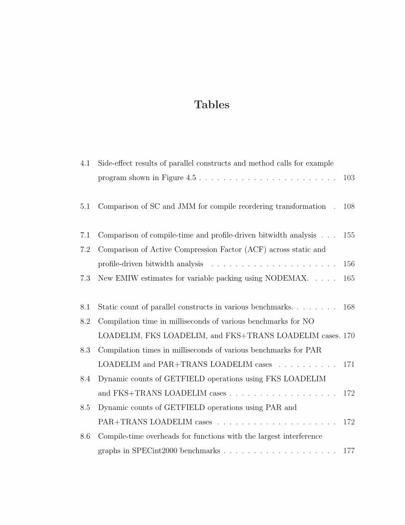
Tables
4.1 Side-effect results of parallel constructs and method calls for example
program shown in Figure 4.5 . . . . . . . . . . . . . . . . . . . . . . . 103
5.1 Comparison of SC and JMM for compile reordering transformation . 108
7.1 Comparison of compile-time and profile-driven bitwidth analysis . . . 155
7.2 Comparison of Active Compression Factor (ACF) across static and
profile-driven bitwidth analysis . . . . . . . . . . . . . . . . . . . . . 156
7.3 New EMIW estimates for variable packing using NODEMAX. . . . . 165
8.1 Static count of parallel constructs in various benchmarks. . . . . . . . 168
8.2 Compilation time in milliseconds of various benchmarks for NO
LOADELIM, FKS LOADELIM, and FKS+TRANS LOADELIM cases. 170
8.3 Compilation times in milliseconds of various benchmarks for PAR
LOADELIM and PAR+TRANS LOADELIM cases . . . . . . . . . . 171
8.4 Dynamic counts of GETFIELD operations using FKS LOADELIM
and FKS+TRANS LOADELIM cases . . . . . . . . . . . . . . . . . . 172
8.5 Dynamic counts of GETFIELD operations using PAR and
PAR+TRANS LOADELIM cases . . . . . . . . . . . . . . . . . . . . 172
8.6 Compile-time overheads for functions with the largest interference
graphs in SPECint2000 benchmarks . . . . . . . . . . . . . . . . . . . 177
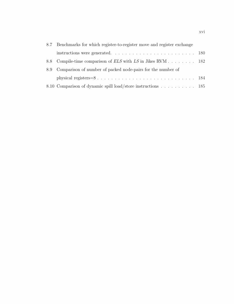
xvi
8.7 Benchmarks for which register-to-register move and register exchange
instructions were generated. . . . . . . . . . . . . . . . . . . . . . . . 180
8.8 Compile-time comparison of ELS with LS in Jikes RVM . . . . . . . . 182
8.9 Comparison of number of packed node-pairs for the number of
physical registers=8 . . . . . . . . . . . . . . . . . . . . . . . . . . . . 184
8.10 Comparison of dynamic spill load/store instructions . . . . . . . . . . 185
1
Chapter 1
Introduction
The computer industry is at a major inflection point in its hardware roadmap due to
the end of a decades-long trend of exponentially increasing clock frequencies. Unlike
previous generations of hardware evolution, the shift towards multicore and manycore
computing will have a profound impact on software — not only will future applications
need to be deployed with sufficient parallelism for manycore processors, but the
parallelism must also be energy-efficient. For decades, caches have helped bridge the
memory wall for programs with high spatial and temporal locality. Unfortunately,
caches come with an energy cost that limits their use as on-chip memory in future
manycore processors. It is therefore desirable for programs to use more energy-
efficient storage structures such as registers and local memories (scratchpads) instead
of caches, as far as possible.
Energy-efficient storage structures offer lower latencies and are faster to access.
However, they are smaller in size and number due to architectural complications
involved in their design. For example, the Intel x86 architecture offers only 8 fixed reg-
isters for integer valued data items. A compiler that converts a higher-level program
into an optimized machine level instruction sequence performs several optimizations in
order to improve the execution performance of a program. One such optimization that
focuses on improving memory accesses in the program is memory-access optimization.
The goal of a memory-access optimization is to promote frequently executed data
values from memory (with higher latency of access) to more efficient structures like
registers and local memories in order to take advantage of their lower latencies and
faster accesses. Several compiler optimizations have been proposed in the literature
2
that address optimization for memory accesses such as scalar replacement [33, 34],
load elimination [52, 75, 102], redundant memory operation analysis [45], and register
promotion [83]. The compiler community has studied these techniques extensively
over three decades and have shown benefits of performing them inside a compiler.
Gordon Moore predicted in 1965 that the number of transistors on a machine
would double every eighteen months. This trend has been observed for a long period
of time. In the past, this increase in the number of transistors (and decrease in
transistor sizes) has led to a corresponding increase in clock frequency. However,
recently, the power wall has caused a trend shift from serial to parallel computing by
introducing more and more low power cores in a processor. All hardware vendors now
ship systems with multi-core processors. The performance gain by the introduction
of multi-core processors is strongly dependent on the software algorithms and their
implementation. For example, in order to achieve speedup on a quad-core machine, it
is necessary to exploit the four cores in software. Hence, new programming languages
like MPI [109], UPC [51], OpenMP [95], Cilk [18], X10 [38], and Titanium [63] have
been developed to expose the available parallelism on a multi-core processor to the
application programmer. Along with new programming languages for parallelism,
there is a need for new compiler techniques to analyze the parallel constructs of
the language and optimize programs keeping parallelism in mind. Currently, most
compilers make conservative assumptions for parallel constructs and hence, miss
several opportunities for code optimization including memory-access optimization.
For example, the Jikes RVM [66] prevents code motion around parallel constructs.
Parallelism poses another challenge to compiler transformations in the form of
interferences among shared data accesses of multiple cores. The legality of a compiler
transformation in the presence of interferences is typically dictated by the underlying
memory model. A memory model determines the set of possible observable behaviors
of the program. A compiler transformation is said to be correct if the set of possible
observable behaviors of the transformed program is a subset of the possible observable
3
behaviors of the original programs. All memory models have the same semantics for a
data-race-free program. However, without prior knowledge, a compile does not know
if the input program is data-race free or not. Hence, it is desirable to define a memory
model for parallel programs that is both programmer and compiler friendly and at the
same time allows for more opportunities for compiler optimizations, which is critical
for program performance. Note that memory-access compiler optimizations are often
viewed as a variant of code reordering transformations, because they can result in a
reordering of load and store instructions, and hence, are correct to perform under a
given memory model.
In conjunction with the hardware trend shift from serial computing to parallel
computing, in dynamic compilation, program execution and compilation can be in-
terleaved. Dynamic compilation is also referred to as Just-In-Time (JIT) compilation
and runtime compilation. For example, the platform-independent bytecodes of a
Java program are usually compiled and executed by a virtual machine that invokes a
JIT compiler. A dynamic compiler shares the common goal of producing optimized
code with that of an offline/static compiler. However, a key difference is that in a
dynamic compiler the compilation time overhead adds to the runtime performance.
The optimizations performed in a dynamic compiler must strike a balance between
performing deeper analysis (with higher complexity) and runtime benefits achieved
from them. In practice, the optimizations must be performed as close to linear time
and space as possible. For example, the Linear Scan register allocation algorithm
proposed by Poletto and Sarkar [100] is performed by many Java virtual machine JIT
compilers due to its linear time and space complexity instead of the Graph Coloring
register allocation approach [25, 28, 35] used in static compilation. However, Linear
Scan is known to lag in runtime performance compared to Graph Coloring approaches.
Thesis Statement: Recent trends in hardware with multi-core processors as
well as software with parallel languages and dynamic compilation have added new
challenges to the Memory Wall problem. Our thesis is that a combination of high-level
4
and low-level compiler optimizations can be effective in addressing these challenges.
The high-level optimizations introduced in this thesis include new approaches to May-
Happen-in-Parallel analysis, Side-Effect analysis, and Scalar Replacement for Load
Elimination transformation for explicitly parallel programs. The low-level dynamic
optimizations include a Space-efficient register allocation algorithm that incurs an
order-of-magnitude smaller compile-time and space overhead than Graph Coloring,
while delivering run-time performance that matches or surpasses that of Graph Col-
oring.
1.1 Research Contributions
This dissertation highlights the challenges in memory-access optimization for parallel
programs, using X10 as an example parallel programming language. The X10 v1.5 lan-
guage [38] builds on a subset of Java language constructs and adds new constructs like
async, finish, atomic, places, region, distribution, and distributed arrays
for supporting fine-grained locality, parallelism and synchronization. Since, version
1.7, X10 has adopted a Scala-like syntax for source code and has introduced new
advances in the type system relative to Java. The Habanero-Java (HJ) programming
language that is being developed in the Habanero Multicore Software Research project
at Rice University focuses on addressing the implementation challenges for the core
constructs of X10 v1.5 language on multi-core processors, with programming model
extensions as needed (such as phasers and isolated blocks). A significant part of
the research results presented in this thesis were obtained for HJ programs.
The dissertation makes the following contributions:
1. a novel May-Happen-in-Parallel (MHP) algorithm for HJ programs that iden-
tifies pairs of execution instances of statements that may execute in parallel.
Compared to past work for other concurrent languages like Java and Ada, we
introduce a more precise definition of the MHP by adding condition vectors
that distinguishes execution instances of statements for which the MHP holds,
5
instead of just returning a single true/false value for all pairs of executing
instances. The availability of basic concurrency control constructs such as
async, finish, isolated and places in HJ enables the use of more efficient
and precise analysis algorithms based on simple path traversals in a Program
Structure Tree.
2. a side-effect analysis for the core parallel constructs of HJ. The side-effect anal-
ysis is designed for dynamically compiling HJ programs and hence, is compile-
time efficient.
3. a novel parallelism-aware scalar replacement transformation for memory load
elimination. The legality of the transformation is established by a new Isolation
Consistency (IC) memory model. Like many relaxed memory models, the
IC memory model provides sequentially consistent behavior for data-race-free
programs. At the same time, IC allows many compiler transformations via
weak-atomicity for programs with data-races.
4. a space-efficient register allocation algorithm that bridges the performance gap
between Linear Scan and Graph Coloring register allocation algorithms while
maintaining the compile-time efficiency of Linear Scan. We model the allocation
phase of a register allocation algorithm as an optimization problem on Bipar-
tite Liveness Graphs (BLG’s), a new data structure introduced in this thesis.
The assignment phase focuses on reducing the number of spill instructions by
using register-to-register move and exchange instructions wherever possible to
maximize the use of registers. The register assignment that includes register-
to-register moves, exchanges, coalescing as well as register class constraints is
modeled as another optimization problem, and we provide a heuristic solution
to this problem as well.
5. an enhanced bitwidth-aware register allocation algorithm that packs several narrow-
width data items onto the same physical register to reduce register pressure of
6
the program. We present an enhanced bitwidth analysis that performs more
detailed scalar analysis and array analysis than past work. We describe an
enhanced packing algorithm that includes more accurate packing and performs
less conservative (more aggressive) coalescing than past work.
1.2 Thesis Organization
• Chapter 2 introduces necessary backgrounds, definitions and notations used in
the thesis. The overall code optimization framework used in the thesis is also
described in this chapter.
• Chapter 3 describes the May-Happens-in-Parallel algorithm for HJ programs.
• Chapter 4 presents the Side-Effect Analysis for parallel constructs and function
calls.
• Chapter 5 describes the Isolation Consistency (IC) memory model and scalar
replacement for load elimination transformation for parallel programs.
• Chapter 6 describes the space-efficient register allocation algorithm and com-
pares it with the graph coloring register allocation.
• Chapter 7 presents our enhancements to bitwidth-aware register allocation al-
gorithm.
• Chapter 8 presents our experimental results.
• Chapter 9 concludes the thesis with a summary and future directions.
7
Chapter 2
Background
In this chapter, we introduce notations and terminologies used in the rest of the
dissertation. First, we describe some basic compiler terminologies. Next, we describe
the HJ parallel programming language. Next, we present our overall code optimization
framework for parallel programs. Finally, we describe the background, foundations
and notations for each of the analyses and optimizations described in our code
optimization framework.
2.1 Basics of a Compiler
A compiler (static or dynamic) typically consists of two components: a front-end and
a back-end. In the front-end, the input program is parsed, represented as an inter-
mediate representation (IR), and transformed. Typical transformations performed in
the front-end are deadcode elimination, constant propagation, copy propagation, and
inlining. After the front-end pass is complete, the back-end component performs
additional transformations that are specific to the target architecture. Typical trans-
formations performed in the back-end are register allocation, instruction scheduling,
and instruction selection. Sometimes compilers add a middle-end that consists of the
transformations of the front-end.
An IR captures the compiler’s knowledge of the input program. It consists of a
set of instructions that correspond to the original input program.
Definition 2.1.1 An instruction defines an operation that possibly reads some vari-
ables and possibly writes some other variables. The variables that are read at an
8
1 a = ...
2 b = true
3 for (i=2; i<a-1; i++) {
4 c = a % i
5 if ( c == 0) {
6 b = false
7 break
8 }
9 }
START
a = ...
b = true
i = 2
i < a - 1
c = a % i
c == 0
i = i + 1
END
B0
B1
B2
B3
B4 B5
b = false
B6
Figure 2.1 : An example control flow graph. The code snippet is shown on the left.The corresponding control flow graph is shown in the right. Note that, the specialbasic blocks START and END are added to demarcate entry and exit to the procedure.
instruction are referred to as used variables and those that are written are referred to
as defined variables.
An IR can be represented in various ways. Some dominant IR representations
are: 1) a linear IR consisting of a linear ordering of instructions, e.g., Java byte-
code; 2) a structural IR consisting of graphical representations of instructions, e.g.,
abstract syntax trees; 3) linear+structural IR consisting of a combination of graphical
representation and linear ordering, e.g., control flow graph (CFG). A CFG-based
representation is widely used for compiler analyses and transformations.
Definition 2.1.2 A control flow graph is a graph, G = 〈V, E〉, where V consists of
basic blocks and E consists of possible execution paths. A basic block is a maximal
sequence of instructions where the execution enters at the first instruction and exits
at the last instruction of the sequence, i.e., there exists no intermediate instruction in
a basic block where an execution can enter or exit. Two special basic blocks START and
END are added to a CFG to indicate the unique entry and unique exit of a procedure.
9
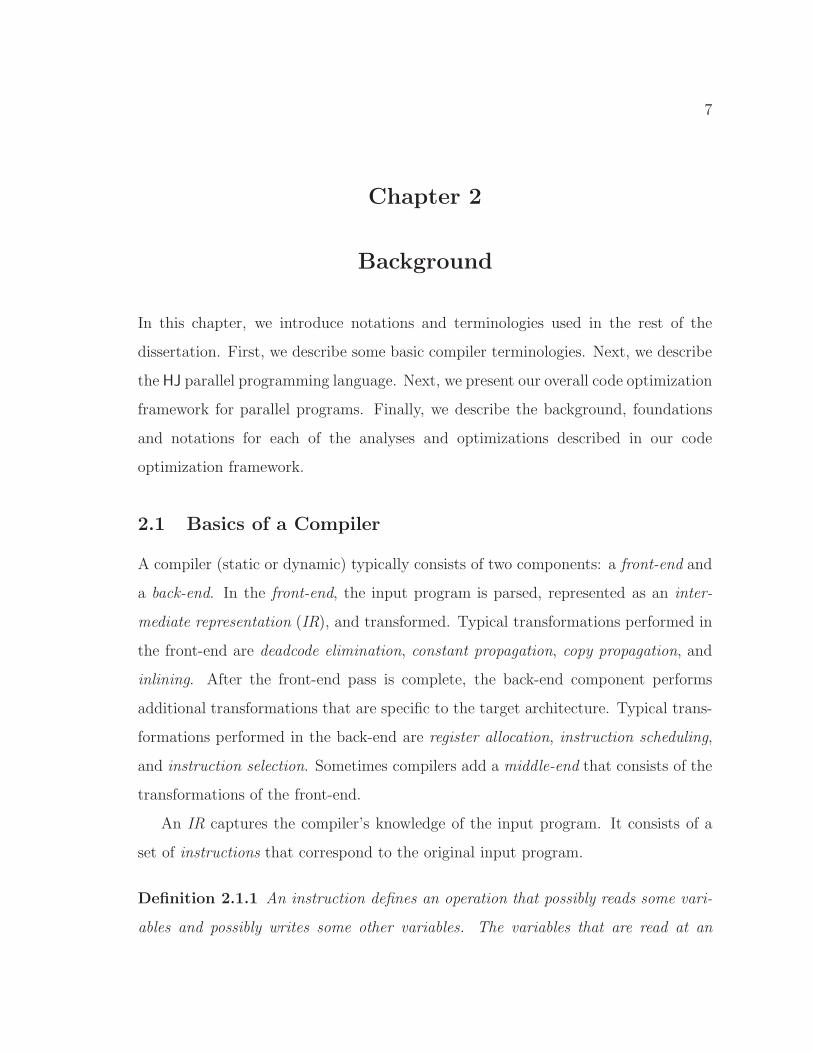
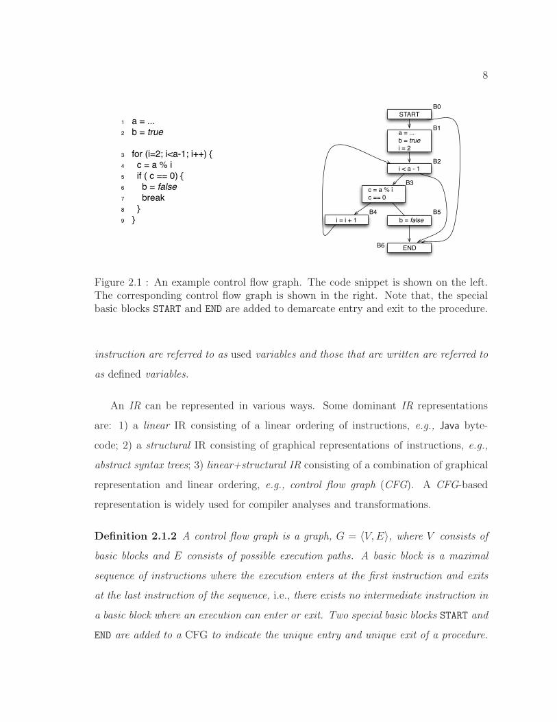
Consider the example program shown in Figure 2.1. The example program com-
putes if a is a prime number or not. The control flow graph (CFG) is shown on the
right. It consists of seven basic blocks, i.e., B0-6, including two special entry and exit
basic blocks B0 and B6, respectively. The basic block B3 consists of two instructions
c = a%i and c == 0. For instruction c = a%i, variables a and i are used whereas c is
defined.
Often it is useful to define dom, idom, and postdom relationships between two
nodes of a CFG.
Definition 2.1.3 Given a CFG, a node x is said to dominate (dom) another node
y if every path from START to y passes through x. Similarly, node x is said to post-
dominate (postdom) node y if every path from y to EXIT passes through x. A node x
is the immediate dominator (idom) of another node y if x dominates y and there is
no intervening node p such that x dom p and p dom y. The idom relation forms a
dominator tree.
For precision, it is often necessary to represent information in between two in-
structions. For example, the liveness of a variable needs to be defined at a program
point rather than at an instruction level.
Definition 2.1.4 A program point is a point between two consecutive instructions.
Definition 2.1.5 A variable v is live at a program point p if ∃ a path in the CFG
(indicating a possible execution) from p to some use of v along which v is not defined
again. As we will discuss in Definition 2.7.5, sometimes it is desired to split a program
point into two sub-program points.
A popular intermediate representation used in the literature is static single as-
signment (SSA) form [47]. In SSA form representation, each variable is defined in
exactly one place in the code. New φ instructions are inserted in the CFG to ensure
that each use of a variable sees exactly one definition. An IR is converted into SSA
10
form using two simple steps: (1) φ-insertion phase: φ statements are inserted at the
iterated dominance frontiers of assignment statements [48]; (2) renaming phase: the
renaming phase assigns unique names using version ids to each variable definition.
Several efficient transformations have been proposed in literature that exploit the
single-assignment property of SSA form such as sparse-conditional constant prop-
agation [122], strength reduction [46], partial redundancy elimination [41] and SSA
based register allocation [29, 59]. We will describe SSA based register allocation in
Section 2.7.2.3.
A common compiler transformation is to find redundant expressions in a program.
An expression a + b is said to be redundant at a program point p if it has already
been computed in every path starting from the START block to p, and no intervening
operation kills either a or b. If the compiler can find such redundant expressions, it
can save the value in a scalar variable at the previous computation and replace any
subsequent computations with the scalar variable. The classic approach to accomplish
this is to use Value Numbering [6]. Value numbering assigns distinct numbers to each
value computed during run time. Two expressions, e1 and e2, have same value number
iff they always compute the same value. We denote the value number of an expression
e as V(e). If the value numbers of two expressions are same, then they are redundant.
An ordering-based compiler transformation such as redundant expression elimina-
tion is said to be correct if it does not violate any dependences. A control dependence
arises from the control flow in the program, where as a data dependence arises from
the flow of values between statements in the program.
Definition 2.1.6 The following types of data dependences exist:
1. Statements S1 and S2 are said to have a flow dependence between them (denoted
as S1δfS2) if S2 uses the value written at S1.
2. Statements S1 and S2 are said to have an anti dependence between them (de-
noted as S1δ−1S2) if S1 uses a value from a location to which S2 writes.
11
3. Statements S1 and S2 are said to have an output dependence between them
(denoted as S1δoS2) if both S1 and S2 write to the same location.
4. Statements S1 and S2 are said to have an input dependence between them
(denoted as S1δiS2) if both S1 and S2 use a value from the same location.
A succinct way of capturing dependences for statements inside a loop is to use
distance and direction vectors.
Definition 2.1.7 Given a dependence from statement S1 on iteration i to statement
S2 on iteration j of a common loop nest l, the direction vector D(i, j) is defined as a
vector of length l such that,
D(i, j)k =
< if jk − ik > 0
= if jk − ik = 0
> if jk − ik < 0
(2.1)
Various dependences between the statements in a program are represented using
a program dependence graph (PDG). PDG’s are used as the foundation for many
compiler reordering transformations such as vectorization, scalar replacement, and
scheduling.
2.2 The HJ Parallel Programming Language
The HJ programming language offers several constructs to improve programmability
in high-performance computing for parallel systems that includes multi-core proces-
sors, symmetric shared-memory multiprocessors (SMPs), commodity clusters, high-
end supercomputers like BlueGene [1], and even embedded processors like Cell [99].
The key features of HJ include:
• Lightweight activities embodied in async, future, foreach, and ateach con-
structs which subsume communication and multithreading operations.
12
• A finish construct for termination detection and rooted exception handling of
descendant activities.
• Support for lock-free synchronization with isolated blocks.
• Explicit reification of locality in the form of places, with support for a parti-
tioned global address space (PGAS) across places.
• Support for collective and point-to-point communication using phaser con-
structs.
HJ uses a serial subset of the Java v1.4 language as its foundation, but replaces the
Java language’s current support for concurrency by new constructs that are motivated
by high-productivity high-performance parallel programming. For further details, the
reader is referred to “An overview of X10 v1.5” [38]. The scope of this dissertation
focuses on four core constructs: async, finish, isolated, and places. Extensions
for the foreach, ateach, and future constructs follow naturally from the approach
described in this thesis, and have been omitted for simplicity. An important safety
result in HJ is that any program written with async, finish, and isolated can never
deadlock.
2.2.1 Single Place HJ Language Constructs
In a single-place HJ program, all activities execute within the same logical place
and have uniform read and write access to all shared data, as in multithreaded Java
programs where all threads operate on a single shared heap.
async 〈stmt〉: Async is the HJ construct for creating or forking a new asyn-
chronous activity. The statement, async 〈stmt〉, causes the parent activity to create a
new child activity to execute 〈stmt〉. Execution of the async statement returns imme-
diately i.e., the parent activity can proceed immediately to the statement following
the async.
13
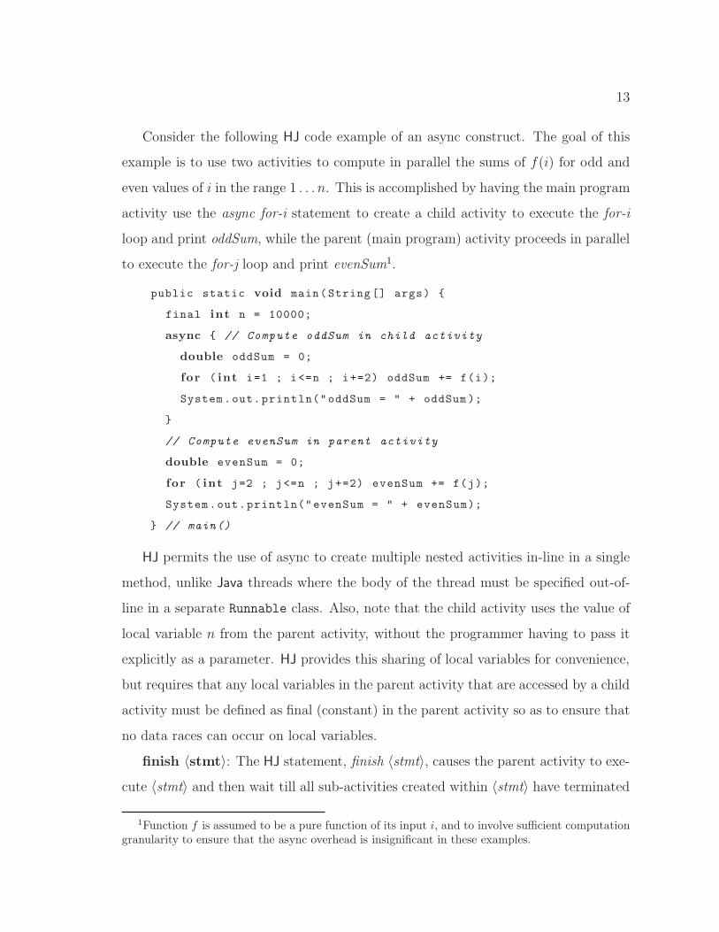
Consider the following HJ code example of an async construct. The goal of this
example is to use two activities to compute in parallel the sums of f(i) for odd and
even values of i in the range 1 . . . n. This is accomplished by having the main program
activity use the async for-i statement to create a child activity to execute the for-i
loop and print oddSum, while the parent (main program) activity proceeds in parallel
to execute the for-j loop and print evenSum1.
public static void main(String [] args) {
final int n = 10000;
async { // Compute oddSum in child activity
double oddSum = 0;
for ( int i=1 ; i<=n ; i+=2) oddSum += f(i);
System.out.println("oddSum = " + oddSum );
}
// Compute evenSum in parent activity
double evenSum = 0;
for ( int j=2 ; j<=n ; j+=2) evenSum += f(j);
System.out.println("evenSum = " + evenSum);
} // main()
HJ permits the use of async to create multiple nested activities in-line in a single
method, unlike Java threads where the body of the thread must be specified out-of-
line in a separate Runnable class. Also, note that the child activity uses the value of
local variable n from the parent activity, without the programmer having to pass it
explicitly as a parameter. HJ provides this sharing of local variables for convenience,
but requires that any local variables in the parent activity that are accessed by a child
activity must be defined as final (constant) in the parent activity so as to ensure that
no data races can occur on local variables.
finish 〈stmt〉: The HJ statement, finish 〈stmt〉, causes the parent activity to exe-
cute 〈stmt〉 and then wait till all sub-activities created within 〈stmt〉 have terminated
1Function f is assumed to be a pure function of its input i, and to involve sufficient computationgranularity to ensure that the async overhead is insignificant in these examples.
14
globally. There is an implicit finish statement surrounding the main program in an
HJ application. If async is viewed as a fork construct, then finish can be viewed as
a join construct. However, the async-finish model is more general than the fork-join
model [38].
HJ distinguishes between local termination and global termination of a statement.
The execution of a statement by an activity is said to terminate locally when the
activity has completed all the computation related to that statement. For example,
the creation of an asynchronous activity terminates locally when the activity has been
created. A statement is said to terminate globally when it has terminated locally and
all activities that it may have spawned (if any) have, recursively, terminated globally.
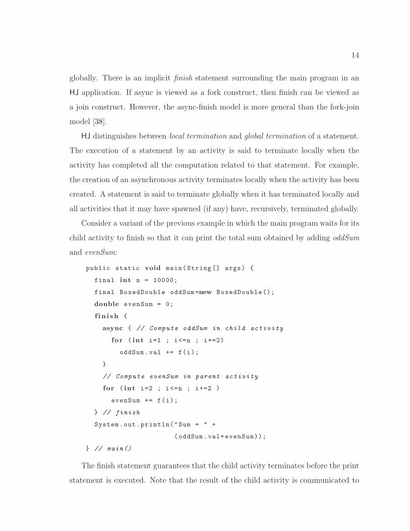
Consider a variant of the previous example in which the main program waits for its
child activity to finish so that it can print the total sum obtained by adding oddSum
and evenSum:
public static void main(String [] args) {
final int n = 10000;
final BoxedDouble oddSum=new BoxedDouble();
double evenSum = 0;
f i n i s h {
async { // Compute oddSum in child activity
for ( int i=1 ; i<=n ; i+=2)
oddSum.val += f(i);
}
// Compute evenSum in parent activity
for ( int i=2 ; i<=n ; i+=2 )
evenSum += f(i);
} // finish
System.out.println("Sum = " +
(oddSum.val+evenSum));
} // main()
The finish statement guarantees that the child activity terminates before the print
statement is executed. Note that the result of the child activity is communicated to
15
the parent in a shared object, oddSum, since HJ does not permit a child activity to
update a local variable in its parent activity.
In addition to waiting for global termination, the finish statement plays an impor-
tant role with regard to exception semantics. An HJ activity may terminate normally
or abruptly. A statement terminates abruptly when it throws an exception that is
not handled within its scope; otherwise it terminates normally. While it may seem
that an obvious solution is to propagate exceptions from a child activity to a parent
activity, doing so is problematic when the parent activity terminates prior to the child
activity. Since we want to permit child activities to outlive parent activities in HJ, the
finish construct is a more natural collection point for exceptions thrown by descendant
activities. HJ requires that if statement S or an activity spawned by S terminates
abruptly, and all activities spawned by S terminate, then finish S terminates abruptly
and throws a single exception formed from the collection of all exceptions thrown by
S or its descendant activities. Exceptions thrown by this statement are caught by the
runtime system and result in an error message printed on the console. This provides
more robust exception handling support for multithreaded programs compared to the
Java model in which an exception is simply propagated from a thread to the top-level
console instead of propagation to an appropriate handler in an ancestor thread.
isolated 〈stmt〉, isolated 〈method-decl〉: An isolated block is executed by an
activity as if in a single step during which all other concurrent activities within the
same place are suspended. The isolated construct is our renaming of X10’s atomic
construct. As stated in [38], an atomic block in X10 is intended to be “executed by an
activity as if in a single step during which all other concurrent activities in the same
place are suspended”. This definition implies a strong atomicity semantics for the
atomic construct. However, all X10 implementations that we are aware of (including
the one used in this paper) use a single lock per place to enforce mutual exclusion
of atomic blocks. This approach supports weak atomicity, since no mutual exclusion
guarantees are enforced between computations within and outside an atomic block.
16
As advocated in [73], we use the isolated keyword instead of atomic to make explicit
the fact that the construct supports weak isolation rather than strong atomicity. An
isolated block may include method calls, conditionals, and other forms of sequential
control flow. Parallel constructs such as async and finish are not permitted in an
isolated block. Isolated blocks may be nested and the isolated modifier on method
definitions are permitted as a shorthand for enclosing the body of the method in
an isolated block. The isolated construct is semantically equivalent to X10’s atomic
construct.
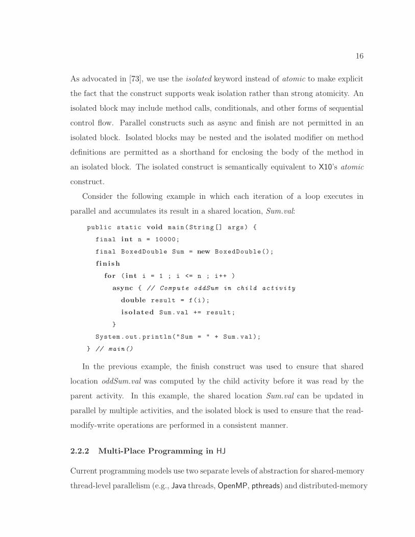
Consider the following example in which each iteration of a loop executes in
parallel and accumulates its result in a shared location, Sum.val:
public static void main(String [] args) {
final int n = 10000;
final BoxedDouble Sum = new BoxedDouble();
f i n i s h
for ( int i = 1 ; i <= n ; i++ )
async { // Compute oddSum in child activity
double result = f(i);
i so lated Sum.val += result;
}
System.out.println("Sum = " + Sum.val);
} // main()
In the previous example, the finish construct was used to ensure that shared
location oddSum.val was computed by the child activity before it was read by the
parent activity. In this example, the shared location Sum.val can be updated in
parallel by multiple activities, and the isolated block is used to ensure that the read-
modify-write operations are performed in a consistent manner.
2.2.2 Multi-Place Programming in HJ
Current programming models use two separate levels of abstraction for shared-memory
thread-level parallelism (e.g., Java threads, OpenMP, pthreads) and distributed-memory
17
Immutable Data - final variables
Partitioned Global Address Space
Place 0 Place MAX_PLACES-1
Remote Async
Activities
Within
Place
Activities
Within
Place
Locally Synchronous
Globally Asynchronous
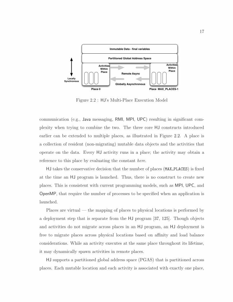
Figure 2.2 : HJ’s Multi-Place Execution Model
communication (e.g., Java messaging, RMI, MPI, UPC) resulting in significant com-
plexity when trying to combine the two. The three core HJ constructs introduced
earlier can be extended to multiple places, as illustrated in Figure 2.2. A place is
a collection of resident (non-migrating) mutable data objects and the activities that
operate on the data. Every HJ activity runs in a place; the activity may obtain a
reference to this place by evaluating the constant here.
HJ takes the conservative decision that the number of places (MAX PLACES) is fixed
at the time an HJ program is launched. Thus, there is no construct to create new
places. This is consistent with current programming models, such as MPI, UPC, and
OpenMP, that require the number of processes to be specified when an application is
launched.
Places are virtual — the mapping of places to physical locations is performed by
a deployment step that is separate from the HJ program [37, 125]. Though objects
and activities do not migrate across places in an HJ program, an HJ deployment is
free to migrate places across physical locations based on affinity and load balance
considerations. While an activity executes at the same place throughout its lifetime,
it may dynamically spawn activities in remote places.
HJ supports a partitioned global address space (PGAS) that is partitioned across
places. Each mutable location and each activity is associated with exactly one place,
18
and places do not overlap. A scalar object in HJ is allocated completely at a single
place. In contrast, the elements of an array, may be distributed across multiple places.
We now discuss how the async and finish constructs discussed earlier in a single-place
context, extend directly to the multi-place case.
2.2.2.1 Remote Asyncs
The statement, async (〈place-expr〉) 〈stmt〉, causes the parent activity to create a
new child activity to execute 〈stmt〉 at the place designated by 〈place-expr〉. The async
is local if the destination place is same as the place where the parent is executing,
and remote if the destination is different. Local async’s are like lightweight threads,
as discussed earlier in the single-place scenario. A remote async can be viewed as
an active message, since it involves communication of input values as well as remote
execution of the computation specified by 〈stmt〉. The semantics of the HJ finish
operator is identical for local and remote async’s viz., to ensure global termination of
all asyncs created in the scope of the finish.
HJ supports a Globally Asynchronous Locally Synchronous (GALS) semantics for
reads/writes to mutable locations. We say that a mutable variable is local for an
activity if it is located in the same place as the activity; otherwise it is remote. An
activity may read/write only local variables (this is called the Locality Rule, and it
may do so synchronously. Any attempt by an activity to read/write a remote mutable
variable results in a BadPlaceException. As mentioned earlier, isolated blocks are
used to ensure atomicity of groups of read/write operations among multiple activities
located in the same place. However, an activity may read/write remote variables only
by spawning activities at their place. Thus a place serves as a coherence boundary in
which all writes to the same datum are observed in the same order by all activities in
the same place. In contrast, inter-place data accesses to remote variables have weak
ordering semantics. The programmer may explicitly enforce stronger guarantees by
using sequencing constructs such as finish.
19
Figure 2.3 : Static and Dynamic Optimization Framework
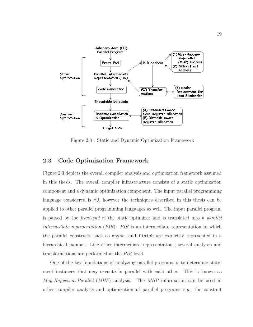
2.3 Code Optimization Framework
Figure 2.3 depicts the overall compiler analysis and optimization framework assumed
in this thesis. The overall compiler infrastructure consists of a static optimization
component and a dynamic optimization component. The input parallel programming
language considered is HJ, however the techniques described in this thesis can be
applied to other parallel programming languages as well. The input parallel program
is parsed by the front-end of the static optimizer and is translated into a parallel
intermediate representation (PIR). PIR is an intermediate representation in which
the parallel constructs such as async, and finish are explicitly represented in a
hierarchical manner. Like other intermediate representations, several analyses and
transformations are performed at the PIR level.
One of the key foundations of analyzing parallel programs is to determine state-
ment instances that may execute in parallel with each other. This is known as
May-Happen-in-Parallel (MHP) analysis. The MHP information can be used in
other compiler analysis and optimization of parallel programs e.g., the constant
20
propagation described in [77] using concurrent-SSA form representation needs to know
the interfering data values and these can be determined using the MHP analysis. In
this thesis, we present a precise definition of MHP using condition vectors that identify
execution instances of statements for which the MHP holds, instead of just returning
a single true/false value for all pairs of executing statement instances. Based on
this definition, we present an efficient algorithm for computing MHP information
for HJ parallel programs. Compared to the MHP analysis of other languages, our
approach [2] is based on a simple walk over the program structure tree which is an
abstraction of the abstract syntax tree. The MHP analysis analyzes async, finish,
isolated, and places constructs of HJ.
Traditionally, procedure calls hinder the precision of compiler transformations in
the absence of interprocedural analysis. Side-effect analysis is an interprocedural
analysis that summarizes the modified and referenced data items for each procedure.
For parallel programs, the parallel constructs themselves embed inherent side-effects.
To enable PIR transformations across procedure boundaries and parallel constructs,
we present a unified side-effect analysis in this thesis that summarizes side-effects of
procedure calls in the presence of parallel constructs. The side-effect analysis [12]
uses a heap-array representation for faster side-effect computation. It computes side-
effects for unique features of HJ programs like global termination using finish and
escaping-async. The side-effects can be used by other code reordering transformations
such as code motion.
After PIR analysis is performed, several PIR transformations are performed. One
such PIR transformation is scalar replacement for load elimination that replaces
memory load operations of object references by scalar variables, thereby enabling
the back-end to generate register accesses instead of load instructions. In this thesis,
we describe a parallelism-aware scalar replacement transformation for eliminating
memory load operations. The legality of such a transformation in parallel programs is
strongly dependent on the underlying memory model supported by the programming
21
language. We describe an Isolation Consistency (IC) memory model [12] for HJ
parallel programs. IC is a weak memory model that allows more opportunities
for code reordering than other existing weaker memory models described in past
work [21, 53, 64, 84]. After transformations are applied at the PIR level, platform-
independent bytecode is produced for the input HJ parallel program.
The other component in our optimization framework is the dynamic optimizer.
The bytecodes produced in the static optimizer are subsequently processed within the
dynamic optimizer framework. Additional higher level and low-level optimizations
are performed at the bytecode level within the dynamic optimizer framework. A
key low-level optimization is register allocation. This thesis makes a contribution
to register allocation optimization by providing an space-efficient register allocation
algorithm [105] that is compile-time efficient and produces comparable executable
code quality as a Graph Coloring based register allocation. The space-efficient register
allocation builds on the notion of intervals with holes used in Linear Scan register
allocation.
One approach to moderate register pressure in a program is to pack several narrow
width data variables into the same physical register. A register allocation algorithm
that is aware of the bitwidth information and performs such a packing is known as
a Bitwidth-aware register allocation algorithm. This thesis makes contributions to
bitwidth-aware register allocation by proposing several enhancements to the compu-
tation of bitwidth information and variable packing heuristic [11].
Finally, the bytecodes are converted to the machine code within the dynamic
optimizer and executed on the target machine.
2.4 May-Happen-in-Parallel (MHP) Analysis
Parallel programming languages offer many high level parallel constructs to create,
synchronize, communicate, and join parallel tasks. All these parallel constructs
indicate the relative progress and interactions of parallel tasks during execution.
22
Further, the interactions among parallel tasks indicate their possible ordering of
execution. For example, the end of a finish scope in HJ ensures the completion
of any parallel task, i.e., async, created within its scope. This implies any async
created after this finish scope will never synchronize/communicate with the asyncs
created with the finish scope.
Knowledge of the possible ordering of parallel tasks has a variety of uses in
the compilation and debugging of parallel programs. These uses include program
debugging tools, data-flow analysis, detecting synchronization anomalies like data-
races and deadlocks [32]. The possible ordering among tasks leads to a problem of
determining the actions that can occur in parallel. This is known in the literature
by several different terms: Concurrency analysis [50, 86], B4 analysis [32], and May-
Happen-in-Parallel analysis [90, 92]. In this thesis, we will use the May-Happen-in-
Parallel (MHP) term. Note that, MHP analysis determines actions that may happen
during execution, i.e., it is may information rather than must information, hence any
query for MHP information can conservatively return true.
Definition 2.4.1 May-Happen-in-Parallel (MHP) analysis statically determines if
it is possible for execution instances of two statements (or the same statement) to
execute in parallel.
The complexity of MHP analysis is highly dependent on the underlying parallel
constructs supported by the programming language. For example, let us consider the
asynchronous parallel loop constructs consisting of parallel DO, parallel case,
POST, and WAIT constructs (described in [68]). Callahan and Sublok [32] have shown
that for a program using the above constructs and without any loop construct, the
MHP computation is NP-hard. Similar complexity results have been proved for Ada’s
rendezvous model of synchronization [118], which is similar to Java’s wait-notify model
of synchronization.
In general, it is safe for a compiler to compute a conservative approximation of
MHP information. For example, Callahan and Sublok [32] proposed a data flow
23
algorithm to compute a conservative approximation of the sets of statements that
must be executed before a given statement (B4 analysis). Most recently, Naumovich
et al. [92] proposed a similar data-flow based algorithm for concurrent Java programs.
2.4.1 MHP Analysis for Java Programs
Java offers parallelism in the form of explicit creation, synchronization, and termina-
tion of threads. Threads can be created using start() method call. Similarly, threads
can be terminated using join(), which is a blocking method call that blocks the parent
thread until the child thread terminates. Interaction among threads can also occur via
synchronized blocks and methods that allow exclusive access to a thread. Monitors
are represented at a higher level using synchronized blocks and are implemented
using locks. Execution inside monitor sections can be interrupted using low-level
synchronization primitives such as wait, notify, and notifyAll.
As discussed in the previous section, MHP analysis of Java programs is NP-hard.
A conservative approximation of MHP analysis for Java programs is provided by
Naumovich et al. [92]. Their approach is based on a data-flow analysis framework
over an interprocedural Parallel Execution Graph (PEG). Below, we summarize their
data flow analysis algorithm.
Definition 2.4.2 A Parallel Execution Graph (PEG), G = 〈N , E〉, where N con-
sists of the set of nodes and E = Econtrol ∪ E thread ∪ Esync. E control consists of the
interprocedural control flow edges. E thread consists of the thread creation edges. Esync
consists of the synchronization edges.
Let O denote the set of objects in the program and T denote the set of threads
in the program. N t comprises of the set of nodes belonging to a thread t ∈ T . M(n)
denotes the MHP information for a n ∈ N , i.e., the set of nodes that may execute
in parallel with n ∈ N . Further, each node n ∈ N has an associated node type, i.e.,
C(n) = {FORK, START,END, JOIN,LOCK,UNLOCK,WAIT,NOTIFY}. tsucc(n)
24
denote the thread creation edge of n, i.e., it comprises of the thread START node
(for the first CFG node of a run method) corresponding to a thread FORK node
(for a thread start node). The edges from FORK nodes to START nodes constitute
E thread. nsucc(n) denotes all the synchronization successors of a NOTIFY node. Note
that a notifyAll construct in Java is translated into a NOTIFY node with multiple
successors. These edges constitute Enotify. W(o) stands for the set of WAIT nodes
corresponding to an object o ∈ O. lnodes(o) denotes the set of nodes n ∈ N such that
n gets executed under a lock on o ∈ O. notifies(n) for a NOTIFY node n ∈ N consists
of the object to which n notifies, e.g., for a node “n:o.notify()”, o ∈ notifies(n).
thread(n) returns the current thread corresponding to n.
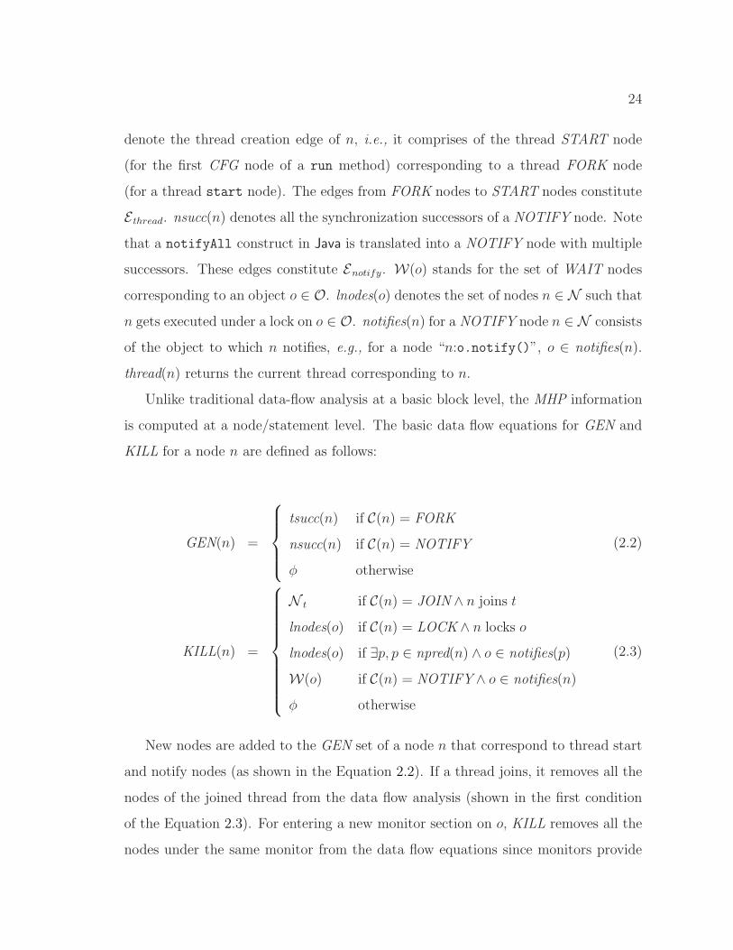
Unlike traditional data-flow analysis at a basic block level, the MHP information
is computed at a node/statement level. The basic data flow equations for GEN and
KILL for a node n are defined as follows:
GEN(n) =
tsucc(n) if C(n) = FORK
nsucc(n) if C(n) = NOTIFY
φ otherwise
(2.2)
KILL(n) =
N t if C(n) = JOIN ∧ n joins t
lnodes(o) if C(n) = LOCK ∧ n locks o
lnodes(o) if ∃p, p ∈ npred(n) ∧ o ∈ notifies(p)
W(o) if C(n) = NOTIFY ∧ o ∈ notifies(n)
φ otherwise
(2.3)
New nodes are added to the GEN set of a node n that correspond to thread start
and notify nodes (as shown in the Equation 2.2). If a thread joins, it removes all the
nodes of the joined thread from the data flow analysis (shown in the first condition
of the Equation 2.3). For entering a new monitor section on o, KILL removes all the
nodes under the same monitor from the data flow equations since monitors provide
25
exclusive access. Similarly, the statements following a WAIT node can not execute in
parallel with any other node under the same monitor on o. Also, none of the WAIT
nodes execute in parallel with any NOTIFY node for the same monitor on o. All
these conditions are shown in Equation 2.3.
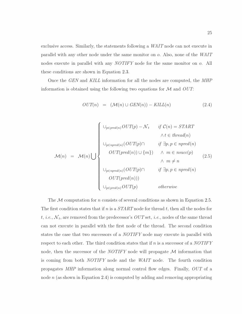
Once the GEN and KILL information for all the nodes are computed, the MHP
information is obtained using the following two equations for M and OUT:
OUT(n) = (M(n) ∪ GEN(n)) − KILL(n) (2.4)
M(n) = M(n)⋃
∪p∈pred(n)OUT(p) −N t if C(n) = START
∧ t ∈ thread(n)
∪p∈npred(n)(OUT(p)∩ if ∃p, p ∈ npred(n)
OUT(pred(n)) ∪ {m}) ∧ m ∈ nsucc(p)
∧ m 6= n
∪p∈npred(n)(OUT(p)∩ if ∃p, p ∈ npred(n)
OUT(pred(n)))
∪p∈pred(n)OUT(p) otherwise
(2.5)
The M computation for n consists of several conditions as shown in Equation 2.5.
The first condition states that if n is a START node for thread t, then all the nodes for
t, i.e., N t, are removed from the predecessor’s OUT set, i.e., nodes of the same thread
can not execute in parallel with the first node of the thread. The second condition
states the case that two successors of a NOTIFY node may execute in parallel with
respect to each other. The third condition states that if n is a successor of a NOTIFY
node, then the successor of the NOTIFY node will propagate M information that
is coming from both NOTIFY node and the WAIT node. The fourth condition
propagates MHP information along normal control flow edges. Finally, OUT of a
node n (as shown in Equation 2.4) is computed by adding and removing appropriating
26
information from M based on GEN and KILL.
Theorem 2.4.3 The data flow equations for M terminates.
Proof: Refer to [92].�
Theorem 2.4.4 The worst-case time complexity of computing M sets for all nodes
in the program is O(N 3) where N denotes the set of nodes in the PEG.
Proof: Refer to [92].�
A practical implementation of the above data flow equations is provided in [81].
Even though the data flow equations are an elegant way of solving the MHP problem,
it has several efficiency and precision problems in the context of Java: 1) the analysis
is closely dependent on an interprocedural alias analysis for thread objects, lock
objects and virtual method calls; 2) the analysis needs explicit enumeration of runtime
threads during compilation time to precisely compute Esync; 3) the analysis has
O(N 3) complexity. If we closely look at the limitation (1), the interprocedural alias
analysis can also benefit from MHP information by eliminating aliases arising from
statements that do not execute in parallel with each other. This causes a cyclic
dependency between MHP analysis and alias analysis. A solution to break the cyclic
dependency may require an incremental analysis between the two causing the overall
complexity to increase and become less practical to perform. To overcome limitation
(2), an abstraction of runtime threads is needed that is aware of runtime threads
created within loops and recursion. This is presented in [10]. Since MHP analysis
involves propagating information at parallel construct boundaries, it’s complexity can
be reduced by computing MHP information at multiple levels, e.g., thread-level and
node-level. Using this approach, a quadratic MHP algorithm is presented in [10].
Chapter 3 of this thesis focuses on MHP analysis for HJ programs. We provide a
precise definition of MHP for statements executed in loops and recursions. Using the
high-level constructs of HJ like finish, async, places, and isolated, an efficient
27
MHP algorithm [2] is described that is linear in complexity and does not involve any
interprocedural alias analysis.
2.5 Side-Effect Analysis
Subroutines (also known as methods, functions and procedures) are a key program-
ming tool in today’s programming languages. They offer several software engineering
benefits including the reduced cost of development and maintenance. For example,
the object-oriented programming in Java consists of two core constructs: objects
and methods. Typically a method consists of a set of parameters, a body, and an
optional return value. When one procedure (the caller) calls another procedure (the
callee), following actions take place in order: 1) binding between formal and actual
parameters; 2) execution of the body of the callee; 3) binding of the return value;
4) return of control to the caller after callee executes. The effect of the callee is
visible to the caller after the call. Side-Effect analysis is a compiler analysis that
determines the effects of a procedure call in an attempt to enhance the opportunities
for optimization. For example, an expression inside a loop containing procedure call
can only be identified as loop-invariant if we knew the side-effects of the procedure
call.
The side effect of a callee consists of the side effect of each statement in the
body of the callee. The term “side effect” was introduced by Spillman [113] for PL/I
programming language. Later on Banning [9] formalized the notion of side-effects for
statements and procedures. We summarize Banning’s side-effect analysis for method
calls as follows.
For a statement s, there are four common types of side effects:
1. MOD(s) consists of the set of variables whose value may be modified by exe-
cuting s.
2. REF(s) consists of the set of variables whose value may be inspected or refer-
28
S2
S1
S1
S2
G1: G
2:
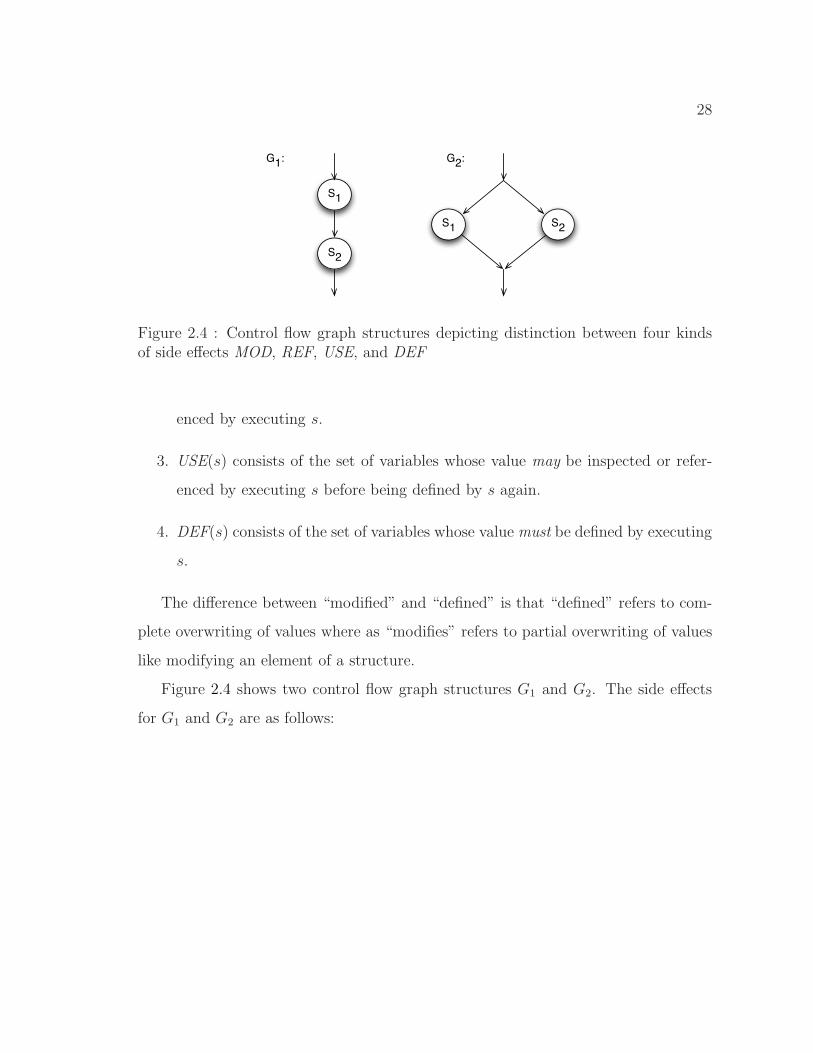
Figure 2.4 : Control flow graph structures depicting distinction between four kindsof side effects MOD, REF, USE, and DEF
enced by executing s.
3. USE(s) consists of the set of variables whose value may be inspected or refer-
enced by executing s before being defined by s again.
4. DEF(s) consists of the set of variables whose value must be defined by executing
s.
The difference between “modified” and “defined” is that “defined” refers to com-
plete overwriting of values where as “modifies” refers to partial overwriting of values
like modifying an element of a structure.
Figure 2.4 shows two control flow graph structures G1 and G2. The side effects
for G1 and G2 are as follows:
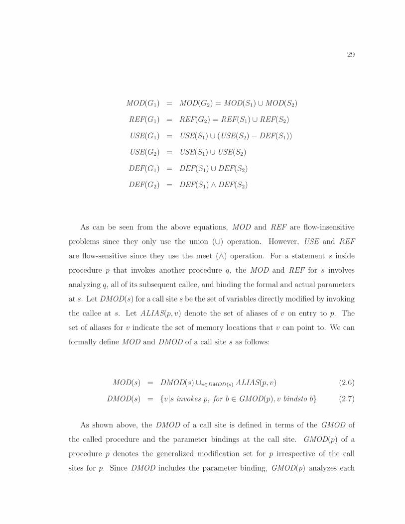
29
MOD(G1) = MOD(G2) = MOD(S1) ∪ MOD(S2)
REF(G1) = REF(G2) = REF(S1) ∪ REF(S2)
USE(G1) = USE(S1) ∪ (USE(S2) − DEF(S1))
USE(G2) = USE(S1) ∪ USE(S2)
DEF(G1) = DEF(S1) ∪ DEF(S2)
DEF(G2) = DEF(S1) ∧ DEF(S2)
As can be seen from the above equations, MOD and REF are flow-insensitive
problems since they only use the union (∪) operation. However, USE and REF
are flow-sensitive since they use the meet (∧) operation. For a statement s inside
procedure p that invokes another procedure q, the MOD and REF for s involves
analyzing q, all of its subsequent callee, and binding the formal and actual parameters
at s. Let DMOD(s) for a call site s be the set of variables directly modified by invoking
the callee at s. Let ALIAS(p, v) denote the set of aliases of v on entry to p. The
set of aliases for v indicate the set of memory locations that v can point to. We can
formally define MOD and DMOD of a call site s as follows:
MOD(s) = DMOD(s) ∪v∈DMOD(s) ALIAS(p, v) (2.6)
DMOD(s) = {v|s invokes p, for b ∈ GMOD(p), v bindsto b} (2.7)
As shown above, the DMOD of a call site is defined in terms of the GMOD of
the called procedure and the parameter bindings at the call site. GMOD(p) of a
procedure p denotes the generalized modification set for p irrespective of the call
sites for p. Since DMOD includes the parameter binding, GMOD(p) analyzes each
30
individual statement in the procedure body using IMOD and each call site in p using
DMOD (recursively). IMOD(p) denotes the set of variables immediately modified
by p (without analyzing the call sites) and is an initial approximation to GMOD.
Formally,
GMOD(p) = IMOD(p) ∪⋃
s invokes q from p
DMOD(s) (2.8)
The equation for GMOD is solved using the reverse call graph of the whole program
until a fixed point is reached. Reverse call graph edges emanate from the callee and
are connected to the caller. Note that if a callee is invoked multiple times from a
caller, multiple edges are added for each invocation of the callee since the parameter
binding in DMOD computation might vary for each invocation of the callee. Each
recursive call path in the program must belong to a strongly connected component
(SCC) in the reverse call graph which can be detected using Tarjan’s depth-first search
algorithm [117]. The SCC is iterated until a fixed point is reached.
The complexity of solving the above data-flow equations for GMOD is O(NEα(E, N)),
where E is the number of call sites in the program, N is the number of procedures
in the program and α represents the inverse Ackermann’s function. The complexity
holds true for all reducible call graphs. The intuition behind the Ackermann’s function
is that the size of the GMOD set grows linearly with respect to the size of the program.
The side-effect computation is a monotonic data flow framework as the GMOD
and GREF sets grow monotonically. According to Kam and Ullman’s theory for
reducible flow graphs [67], the complexity of side-effect computation should have
been bounded by the loop connectedness of the reverse call graph. However, Cooper
and Kennedy [43] observed that for a single recursive procedure program where the
first parameter is modified before the recursive call with rest of the parameters (as
shown in Figure 2.5), the complexity of the side-effect computation is bounded by
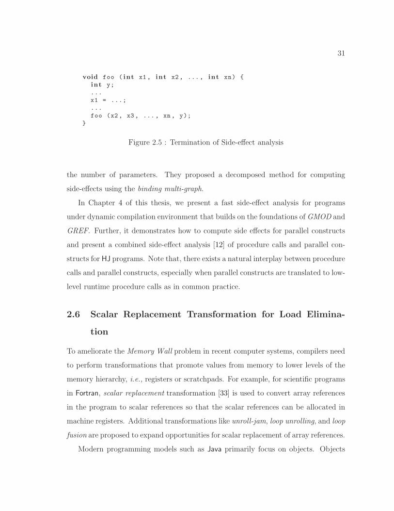
31
void foo ( int x1 , int x2, ..., int xn) {
int y;
...
x1 = ...;
...
foo (x2 , x3 , ..., xn , y);
}
Figure 2.5 : Termination of Side-effect analysis
the number of parameters. They proposed a decomposed method for computing
side-effects using the binding multi-graph.
In Chapter 4 of this thesis, we present a fast side-effect analysis for programs
under dynamic compilation environment that builds on the foundations of GMOD and
GREF. Further, it demonstrates how to compute side effects for parallel constructs
and present a combined side-effect analysis [12] of procedure calls and parallel con-
structs for HJ programs. Note that, there exists a natural interplay between procedure
calls and parallel constructs, especially when parallel constructs are translated to low-
level runtime procedure calls as in common practice.
2.6 Scalar Replacement Transformation for Load Elimina-
tion
To ameliorate the Memory Wall problem in recent computer systems, compilers need
to perform transformations that promote values from memory to lower levels of the
memory hierarchy, i.e., registers or scratchpads. For example, for scientific programs
in Fortran, scalar replacement transformation [33] is used to convert array references
in the program to scalar references so that the scalar references can be allocated in
machine registers. Additional transformations like unroll-jam, loop unrolling, and loop
fusion are proposed to expand opportunities for scalar replacement of array references.
Modern programming models such as Java primarily focus on objects. Objects
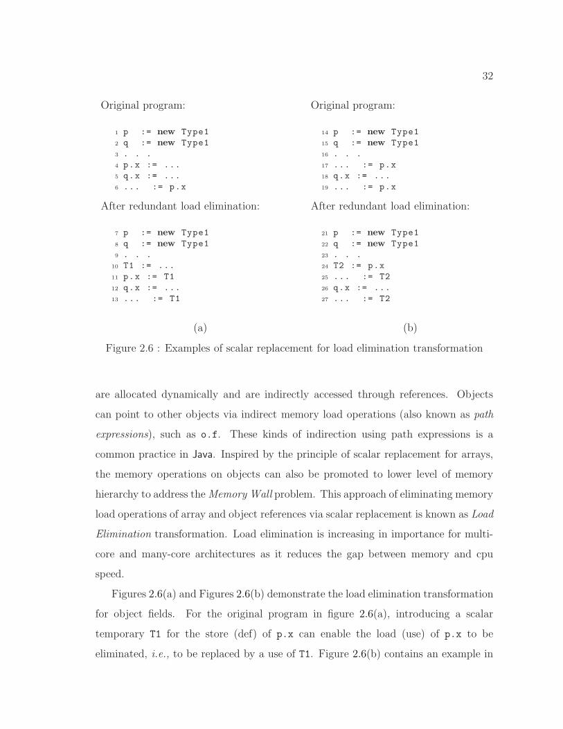
32
Original program:
1 p := new Type1
2 q := new Type1
3 . . .
4 p.x := ...
5 q.x := ...
6 ... := p.x
After redundant load elimination:
7 p := new Type1
8 q := new Type1
9 . . .
10 T1 := ...
11 p.x := T1
12 q.x := ...
13 ... := T1
(a)
Original program:
14 p := new Type1
15 q := new Type1
16 . . .
17 ... := p.x
18 q.x := ...
19 ... := p.x
After redundant load elimination:
21 p := new Type1
22 q := new Type1
23 . . .
24 T2 := p.x
25 ... := T2
26 q.x := ...
27 ... := T2
(b)
Figure 2.6 : Examples of scalar replacement for load elimination transformation
are allocated dynamically and are indirectly accessed through references. Objects
can point to other objects via indirect memory load operations (also known as path
expressions), such as o.f. These kinds of indirection using path expressions is a
common practice in Java. Inspired by the principle of scalar replacement for arrays,
the memory operations on objects can also be promoted to lower level of memory
hierarchy to address the Memory Wall problem. This approach of eliminating memory
load operations of array and object references via scalar replacement is known as Load
Elimination transformation. Load elimination is increasing in importance for multi-
core and many-core architectures as it reduces the gap between memory and cpu
speed.
Figures 2.6(a) and Figures 2.6(b) demonstrate the load elimination transformation
for object fields. For the original program in figure 2.6(a), introducing a scalar
temporary T1 for the store (def) of p.x can enable the load (use) of p.x to be
eliminated, i.e., to be replaced by a use of T1. Figure 2.6(b) contains an example in
33
which a scalar temporary (T2) is introduced for the first load of p.x, thus enabling
the second load of p.x to be eliminated, i.e., replaced by T2. The load elimination
transformations in Figures 2.6(a) and 2.6(b) are correct because p and q have different
values thus ensuring that the store of q.x does not interfere with p.x.
Scalar replacement [33] studied in the context of register reuse leads to load
elimination as the two scenarios described above are exactly same as the reuse due
to flow and input dependencies that a scalar replacement addresses. However, load
elimination needs additional mechanisms for disambiguating object references that
scalar replacement did not address.
There has been much past work on load elimination via scalar replacement in-
cluding [19, 20, 33, 45, 52, 75, 82, 83, 102]. We now summarize the load elimination
algorithm presented by Fink et al. [52] as it is assumed as a baseline for our work on
load elimination in parallel programs.
2.6.1 Unified Modeling of Arrays and Objects
As described in Fink et al. [52], accesses to object fields and array elements in the
program can be represented using hypothetical heap arrays that are compile-time
abstractions of the runtime heap. Each object field x in the program is abstracted by
a distinct heap array, Hx. Hx represents all the instances of field x in the heap. A use
of a.x is represented as a use of element Hx[a], and a definition of b.x is represented
as a def of element Hx[b]. The use of heap arrays ensures that field x is considered
to be the same across instances of two different static types T1 and T2, if (say) T1 is
a subtype of T2. It also ensures disambiguation of memory accesses to distinct fields,
since they will be converted to accesses to distinct heap arrays.
Likewise, each array is abstracted as a two dimensional heap array with one
dimension representing object reference and the second dimension represented by the
subscript. We use the notation HT []R to denote a heap array whose dimensionality
(rank) is R and element type is T . Note that distinct heap arrays are created for
34
each distinct array type in the source program, e.g., Hi[]R represents integer arrays.
2.6.2 Extended Array SSA form
The arrays and object references in the IR can be renamed with the heap array
representation described above to build an extended version of Array SSA form [69].
This involves inserting two specialized φ functions for use and def of heap arrays apart
from the standard SSA form based φ functions. Each definition of a heap variable
is replaced with a definition φ (dφ) that indicates a merge function to merge the old
values with the partial modification in the current definition statement. For example,
for a[i] = ..., only i-th element is modified keeping other elements of array a intact.
Similarly, each use of a heap variable is replaced with a use φ (uφ) to link multiple
loads for the same heap array in control flow order. For each dφ and uφ instructions
that are added to the IR, new φ instructions are added at their respective iterated
dominance frontier to keep the program in SSA form.
2.6.3 Load Elimination Algorithm
For eliminating redundant loads, we need a way of distinguishing heap variables
Hx[a] for a.x and Hx[b] for b.x. This is described using the definitely-same and
definitely-different relations.
Definition 2.6.1 Hx[a] and Hx[b] are definitely same (DS) if a and b have same
values at all program points that are dominated by the definition of a and dominated
by the definitions of b. This information can be obtained using value numbers of a
and b, i.e., V(a) = V(b), where V(a) represents the value number associated with a.
Note that DS is a transitive relation.
Definition 2.6.2 Hx[a] and Hx[b] are definitely different (DD) if a and b have
distinct values at all program points that are dominated by the definition of a and
dominated by the definitions of b. Note that DD is not a transitive relation.
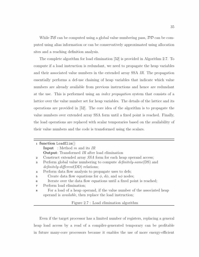
35
While DS can be computed using a global value numbering pass, DD can be com-
puted using alias information or can be conservatively approximated using allocation
sites and a reaching definition analysis.
The complete algorithm for load elimination [52] is provided in Algorithm 2.7. To
compute if a load instruction is redundant, we need to propagate the heap variables
and their associated value numbers in the extended array SSA IR. The propagation
essentially performs a def-use chaining of heap variables that indicate which value
numbers are already available from previous instructions and hence are redundant
at the use. This is performed using an index propagation system that consists of a
lattice over the value number set for heap variables. The details of the lattice and its
operations are provided in [52]. The core idea of the algorithm is to propagate the
value numbers over extended array SSA form until a fixed point is reached. Finally,
the load operations are replaced with scalar temporaries based on the availability of
their value numbers and the code is transformed using the scalars.
function LoadElim()1
Input : Method m and its IROutput: Transformed IR after load eliminationConstruct extended array SSA form for each heap operand access;2
Perform global value numbering to compute definitely-same(DS) and3
definitely-different(DD) relations;Perform data flow analysis to propagate uses to defs;4
Create data flow equations for φ, dφ, and uφ nodes;5
Iterate over the data flow equations until a fixed point is reached;6
Perform load elimination;7
For a load of a heap operand, if the value number of the associated heap8
operand is available, then replace the load instruction;
Figure 2.7 : Load elimination algorithm
Even if the target processor has a limited number of registers, replacing a general
heap load access by a read of a compiler-generated temporary can be profitable
in future many-core processors because it enables the use of more energy-efficient
36
and scalable storages like registers and local memories (scratchpads). Performing
such scalar replacement for load elimination in parallel programming languages for
multi/many-core processors pose additional challenges in the form of interferences
among shared data accesses across parallel tasks. These interferences are commonly
known as data races. Analyzing programs with or without data races is strongly
tied to the underlying memory model supported by the language. Chapter 5 of
this dissertation describes a parallelism-aware scalar replacement algorithm for load
elimination transformation [12] whose legality is provided using a new weak memory
model called Isolation Consistency (IC).
2.7 Register Allocation
The Register file is the most critical storage resource in a computer’s processing unit.
It contains a limited number of physical machine registers and provides faster access
to operands than any other storage resource in a computer. For example, the x86
architecture provides 8 fixed machine registers and multiple of these registers can be
accessed in one cycle. Hence, it is important from an optimizing compiler’s perspective
that the utilization of the register file be controlled. Register Allocation is a compiler
back-end phase that maps operands to physical registers at various program points.
Operands are either program variables or compiler generated temporaries. We use
variables, symbolic registers, and operands, interchangeably. Since the number of
physical registers is usually smaller than the number of simultaneously live variables,
it is almost always the case that some of the operands need to be spilled, i.e., allocated
in other resources like cache, memory, or scratchpads.
Given k physical registers, a register allocation problem can be formally stated as
follows:
Definition 2.7.1 Given a set of variables V and k physical registers, determine if it
is possible to assign each variable v ∈ V to a physical register at each program point
where v is live. If so, rewrite the code using physical registers. Otherwise, rewrite the
37
code using spill code.
Typically, a register allocator consists of two tasks: allocation and assignment.
Allocation determines which operands should be held in physical machine registers
at various program points and which operands should be “spilled”. Assignment
identifies which specific machine registers of the target machine should be used at
different program points to hold which operands. While allocation ensures that no
more than k variables are residing in registers at any program point (where k is
the total number of physical registers available in the target machine), assignment
produces the actual register names required in the executable code. Both these tasks
are equally difficult, i.e., NP-hard to perform at all levels of compilations including
local (basic block level), global (procedure level) and interprocedural (whole-program
level)2. Modern architectural innovations like register classes, register aliasing, and
register pairs further complicate the register allocation problem.
In the rest of the section, we first summarize common terminology used in register
allocation and describe several existing techniques for register allocation.
2.7.1 Terminology
2.7.1.1 Liveness, Live-ranges and Interference Graph
For register allocation, it is necessary to know which variables can be allocated to
the same physical register and which can not. This information is usually abstracted
away in the form of live-ranges and interference. Based on the notion of liveness and
program point described in Section 2.1, we can define the live-range of a variable and
the interference of two variables as follows:
Definition 2.7.2 The live-range of a variable v denoted as lr(v) is the set of program
points where v is live.
2It is possible to perform optimal allocation for a single basic block [14, 44, 88]

38
Definition 2.7.3 Two variables a and b are said to be interfering (or conflicting)
with each other if lr(a) ∩ lr(b) 6= φ.
The live-ranges in a program can be computed using the algorithms presented
in [8, 24]. The interference among all program variables can be represented using an
undirected graph known as the interference graph.
Definition 2.7.4 The interference graph (IG) is a graph, G = 〈V, E〉, where V con-
sists of variables and E consists of edges between variables arising from interference,
i.e., two interfering variables a and b will have an edge between them.
The IG serves as the main data structure of all register allocation algorithms based
on graph coloring. Hence it is critical to represent an interference graph efficiently.
Usually IG is implemented using two representations: 1) bit matrix: that supports
constant time implementation of determining interference between two variables; 2)
adjacency list: consists of a list of adjacent neighbors for every node in IG and
supports fast iteration over the neighbors. The worst-case space complexity of an IG
is O(n2), where n is the total number of variables in the IR.
2.7.1.2 Spilling
Spilled variables incur the additional cost of load and store memory operations
for transferring values between registers and memory. These memory operations
constitute spill code and are usually expensive. Hence, a register allocator should
always aim to keep the frequently-used values in registers to minimize the impact of
spill code.
2.7.1.3 Coalescing
The IR undergoes several front-end transformations before back-end register alloca-
tion pass of the compiler. One particular instruction that occurs frequently in the IR
after compiler transformation is a move instruction of the form “dest = src” as move
39
src,dest. From a register allocation perspective, if src and dest are assigned to the same
physical register (also known as coalesced), then the move instruction can be removed
from the IR. However, when the live-ranges of src and dest interfere with each other,
it may not be possible to assign src and dest the same physical register. Since the
ultimate goal of register allocation is to produce efficient code, a register allocation
algorithm needs to optimize away as many move IR instructions as possible. Several
coalescing techniques have been proposed in the literature: aggressive coalescing [35],
conservative coalescing [28], optimistic coalescing [96], and iterated coalescing [57].
Recently, [23] have shown that all the above coalescing techniques are NP-hard.
2.7.1.4 Live-range splitting
Sometimes it may be beneficial to split the live-range of a variable into two or more
smaller live-ranges. The smaller live-ranges can be separately allocated to memory or
physical registers after variable renaming. This is helpful especially when a live-range
can be assigned a physical register in some program points instead of the whole live-
range. The down-side of live-range splitting is that it incurs extra cost of inserting
move and load/store instructions among smaller live-ranges.
2.7.1.5 Architectural Considerations
Register Classes: Typically, a register allocation problem is stated using a set of
k uniform physical registers. These k registers are assumed to be independent and
interchangeable. Independent means that modifying one physical register does not
modify another and interchangeable means that they can be exchanged with each
other in a particular context. However, modern systems come with physical registers
which may not necessarily be interchangeable. For example, the Intel x86 architecture
provides eight integer physical registers, of which six are usable by the compiler. These
six physical registers are further divided into four high level register classes based on
calling conventions and 8-bit operand accesses. Similarly, for most architectures the
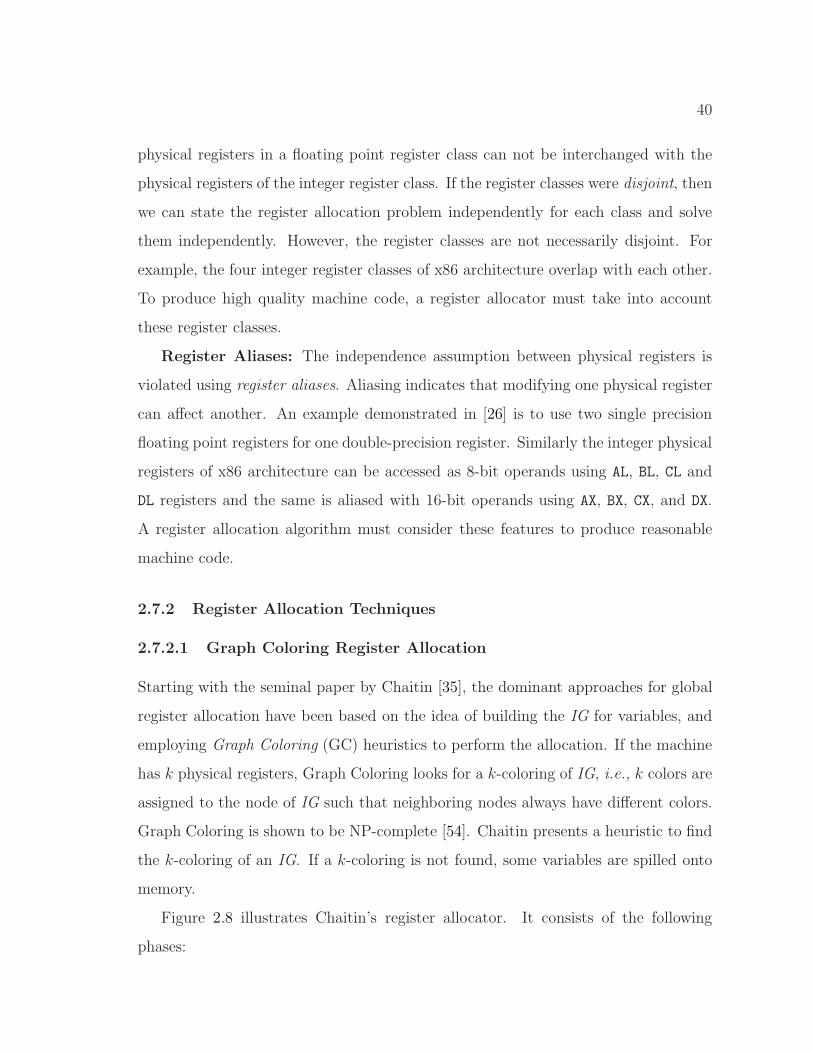
40
physical registers in a floating point register class can not be interchanged with the
physical registers of the integer register class. If the register classes were disjoint, then
we can state the register allocation problem independently for each class and solve
them independently. However, the register classes are not necessarily disjoint. For
example, the four integer register classes of x86 architecture overlap with each other.
To produce high quality machine code, a register allocator must take into account
these register classes.
Register Aliases: The independence assumption between physical registers is
violated using register aliases. Aliasing indicates that modifying one physical register
can affect another. An example demonstrated in [26] is to use two single precision
floating point registers for one double-precision register. Similarly the integer physical
registers of x86 architecture can be accessed as 8-bit operands using AL, BL, CL and
DL registers and the same is aliased with 16-bit operands using AX, BX, CX, and DX.
A register allocation algorithm must consider these features to produce reasonable
machine code.
2.7.2 Register Allocation Techniques
2.7.2.1 Graph Coloring Register Allocation
Starting with the seminal paper by Chaitin [35], the dominant approaches for global
register allocation have been based on the idea of building the IG for variables, and
employing Graph Coloring (GC) heuristics to perform the allocation. If the machine
has k physical registers, Graph Coloring looks for a k-coloring of IG, i.e., k colors are
assigned to the node of IG such that neighboring nodes always have different colors.
Graph Coloring is shown to be NP-complete [54]. Chaitin presents a heuristic to find
the k-coloring of an IG. If a k-coloring is not found, some variables are spilled onto
memory.
Figure 2.8 illustrates Chaitin’s register allocator. It consists of the following
phases:

41
1. Renumber renames live ranges. It creates a new live range for each definition of
a variable. At each use of a variable, it combines the live ranges that reach the
use.
2. Build constructs the IG.
3. Coalesce combines two non-interfering live ranges that are part of a move
instruction. When two live ranges are coalesced, new live ranges are created
and hence, IG is updated. Chaitin’s coalescing approach did not consider the
decrease/increase of the colorability of IG after coalescing. Hence, Chaitin’s
coalescing is commonly referred to as aggressive coalescing [35].
4. Spillcost computes the compiler’s estimation of run-time cost of a live range
when the live range is spilled onto memory.
5. Simplify removes nodes from the IG and creates an ordering of the nodes using a
stack. If the degree of a node is less than k, the node and its edges are removed
from IG and pushed onto the stack. If there are no nodes in the IG that have
degree less than k, then a node is chosen for spilling. After all the nodes are
removed from the IG, spill code is added for the spilled nodes and the register
allocation process is repeated from the beginning.
6. Spill code inserts appropriate load and store memory operations for spilled live
ranges.
7. Select assigns colors to the nodes in the order specified by the stack in Simplify
pass.
The above heuristic leverages the observation that when a node with degree less
than k is removed from the IG, the k-colorability of IG is not changed. Nodes with
degree greater than or equal to k are spilled. The node selection for spilling is based
on the smallest ratio of spill cost divided by the degree.
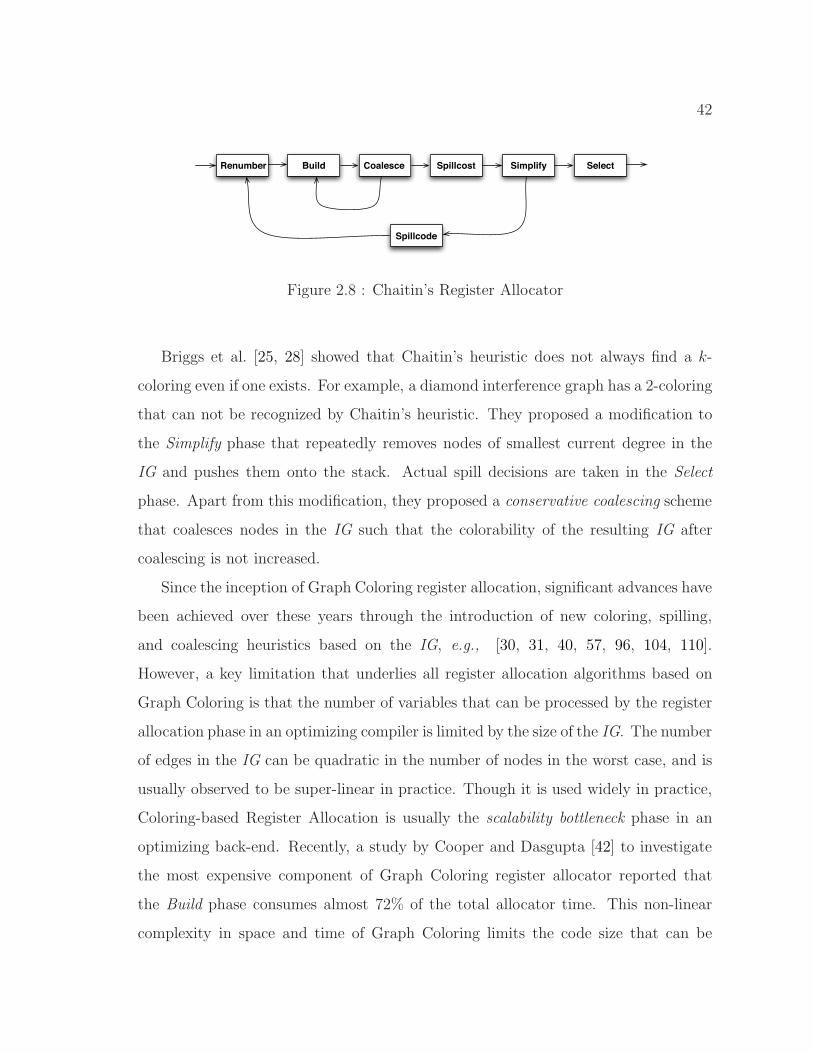
42
Renumber Build Coalesce Spillcost Simplify Select
Spillcode
Figure 2.8 : Chaitin’s Register Allocator
Briggs et al. [25, 28] showed that Chaitin’s heuristic does not always find a k-
coloring even if one exists. For example, a diamond interference graph has a 2-coloring
that can not be recognized by Chaitin’s heuristic. They proposed a modification to
the Simplify phase that repeatedly removes nodes of smallest current degree in the
IG and pushes them onto the stack. Actual spill decisions are taken in the Select
phase. Apart from this modification, they proposed a conservative coalescing scheme
that coalesces nodes in the IG such that the colorability of the resulting IG after
coalescing is not increased.
Since the inception of Graph Coloring register allocation, significant advances have
been achieved over these years through the introduction of new coloring, spilling,
and coalescing heuristics based on the IG, e.g., [30, 31, 40, 57, 96, 104, 110].
However, a key limitation that underlies all register allocation algorithms based on
Graph Coloring is that the number of variables that can be processed by the register
allocation phase in an optimizing compiler is limited by the size of the IG. The number
of edges in the IG can be quadratic in the number of nodes in the worst case, and is
usually observed to be super-linear in practice. Though it is used widely in practice,
Coloring-based Register Allocation is usually the scalability bottleneck phase in an
optimizing back-end. Recently, a study by Cooper and Dasgupta [42] to investigate
the most expensive component of Graph Coloring register allocator reported that
the Build phase consumes almost 72% of the total allocator time. This non-linear
complexity in space and time of Graph Coloring limits the code size that can be
43
optimized and thereby has a damping effect on aggressive use of code transformations
that can potentially increase opportunities for register allocation, such as variable
renaming, loop unrolling and procedure inlining, but which also have the side effect of
increasing the size of the IG. Finally, the non-linear complexity makes it prohibitive
to use Graph Coloring for register allocation in just-in-time and dynamic compilers,
where compile-time overhead contributes directly to runtime.
2.7.2.2 Linear Scan Register Allocation
Just-in-Time (JIT) compilation performed by dynamic compilers aim at compiling
codes on the fly, i.e., compilation happens while the code executes. This adds extra
constraints in terms of time and space than static compilation. Past work by [100, 101]
introduce a new register allocation algorithm, the “linear scan” register allocation.
Their proposed algorithm is fast as it makes a single pass over the IR instructions and
requires very little space since it does not build the interference graph explicitly. Due
to its lightweight nature, Linear Scan has been used in many state-of-the-art Virtual
Machines such as HotSpot Client Compiler [70], LLVM [74], and Jikes RVM [66].
Linear scan assumes a linear ordering of the IR instructions. The choice of ordering
affects the quality of allocation but not the correctness. There are several possible
orderings, such as the original order in which instructions appear in IR (linear order)
and a depth-first ordering over the control flow graph. It has been observed by Poletto
and Sarkar [100] that both linear and depth-first order produce similar code. In the
rest of the thesis, we will consider depth-first ordering.
Definition 2.7.5 Each program point i is represented with i− and i+, where i−
consists of the variables that are read at i and i+ consists of the variables that are
written at i. i− and i+ are represented in integer numbers based on the order of the
IR instructions.
Like live ranges in graph coloring register allocation, the central data structure in
44
linear scan is the notion of a live interval. According to the original notion described
in [100], a live interval is defined as follows:
Definition 2.7.6 An integer range [x, y] is a live interval for a variable v iff ∄p, such
that
1. p < x and v is live at p, or,
2. p > y, v is live at p.
For [x, y], x is referred to as the unique start point (denoted as Lo(v)) and y is referred
to as the unique end point (denoted as Hi(v)).
The above definition permits a live interval to include program points where a
variable v may not be live. The sub-interval during which a variable is not live is
known as a life-time hole [119]. It is important to consider life-time holes in linear
scan as it is possible that two overlapping intervals (according to the above definition
of live intervals) can be allocated to the same physical register if both of them are
not live simultaneously. To distinguish between live intervals and live intervals with
holes, let us define basic interval (BI) and compound interval (CI).
Definition 2.7.7 [x, y] is a basic interval (BI) for variable v iff ∀p, x ≤ p ≤ y, v is
live at p. Note that a BI does not allow any life-time hole. Lo(b) and Hi(b) denote
the unique start and end points of interval b, respectively.
Definition 2.7.8 A compound interval (CI) for a variable v consists of a set of
disjoint basic intervals for v. Note that, a CI permits life-time holes.
From a register allocation perspective, it is required to decide those BIs that
need to be in physical registers and those CIs that need to be spilled3. Register
3Spilling at a compound interval level permits all-or-nothing or spill everywhere approach. In therest of the dissertation, we will focus on this approach instead of partial spills.
45
assignment decides the exact mapping of BI to physical registers. Given that each
BI is represented using a unique start and end point, the register allocation problem
can be viewed as an interval graph coloring problem. Formally,
Definition 2.7.9 An interval graph is a graph, G = 〈V, E〉, where V consists of the
set of BIs and E consists of the intersecting BIs.
Definition 2.7.10 Two BIs, [x1, y1] and [x2, y2], are said to be intersecting if one of
the the following holds:
1. x2 ≥ x1 and x2 ≤ y1
2. y2 ≥ x1 and y2 ≤ y1
Theorem 2.7.11 An interval graph G = 〈V, E〉 can be colored optimally in linear
time.
Proof: Refer to [88, 94].�
The optimal interval graph coloring described in [94] consists of the following steps:
1) find an ordering of the intervals based on increasing Hi values4; 2) Assign color
to an interval by looking at the already colored adjacent nodes (or neighbors) in the
interval graph. Readers are encouraged to see [88, 94] for more details.
Linear Scan register allocation [100] follows the basic theme of interval graph
coloring described above. However, it brings important implementation efficiencies to
ensure smaller time and space requirements. Like interval graph coloring, linear scan
sorts the basic intervals in increasing order of Lo. Instead of building the interval
graph explicitly, it maintains an active list of basic intervals that orders the basic
intervals in increasing order of Hi. Note that, the active list plays the role of already
colored adjacent nodes (or neighbors) in interval graph coloring. The reason the
active list is sorted in increasing order of end points is two fold: 1) For efficiency
4One particular order either increasing or decreasing should be considered
46
reasons, linear scan performs allocation and assignment in a single pass over the
interval start points. Hence, it is necessary to decide spilled intervals while allocation
is being performed. Using the farthest-use approach of Belady [14], linear scan decides
intervals that have largest end point in active list for spilling; 2) While basic intervals
expire (create life-time holes), they are removed from active list. The scan to remove
basic intervals from active list stops as soon as the current intervals start point is
reached.
The complete linear scan algorithm is presented in Algorithm 2.9. Step 2 builds
a sorted set of BIs based on increasing start points. Step 3 initializes the active list
ActiveSet to φ. Step 4 iterates over sorted basic intervals and at each BI’s start
point, it makes the allocation and assignment decisions. In Step 5, the function
Expire removes basic intervals from ActiveSet whose end points (i.e., Hi) are less
than the current BI’s start point. If at any point the size of the ActiveSet is equal to
the number of physical registers (k), then a spill candidate is chosen based on interval
end points (this is shown in Step 6). Step 9 assigns the specific physical register to
an interval. Finally, the current BI is added to the ActiveSet.
Now let us discuss about the complexity of Algorithm 2.9. The overall complexity
is bounded by the following steps: 1) Step 4; 2) the time to add an interval to
ActiveSet; 3) Step 13. Let us assume that there are |BI| number of basic intervals
that arise from V variables. Let there be k number of physical registers. Further,
let the ActiveSet be implemented using a binary search tree, i.e., the time to add an
interval to ActiveSet is log k. Step 4 takes O(|BI|) time. Step 13 takes O(k) time.
So the overall complexity is O(|BI| ∗ (k + log k)).
Let us consider the example program shown in Figure 2.10. Variable a is initialized
before the if-else construct and is used inside both the branches but not after the merge
point. This gives rise to two contiguous basic intervals for a when the code is ordered
in the sequence shown on the left, i.e., CI(a) = {[1+, 4−], [8−, 11−]}. Note that, CI(a)
includes hole in between the basic intervals. The compound intervals of b and c consist
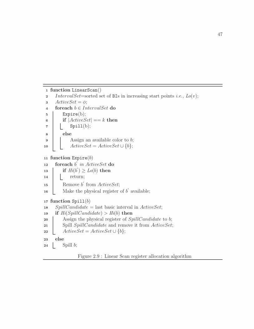
47
function LinearScan()1
IntervalSet=sorted set of BIs in increasing start points i.e., Lo(v);2
ActiveSet = φ;3
foreach b ∈ IntervalSet do4
Expire(b);5
if |ActiveSet| == k then6
Spill(b);7
else8
Assign an available color to b;9
ActiveSet = ActiveSet ∪ {b};10
function Expire(b)11
foreach b′
in ActiveSet do12
if Hi(b′
) ≥ Lo(b) then13
return;14
Remove b′
from ActiveSet;15
Make the physical register of b′
available;16
function Spill(b)17
SpillCandidate = last basic interval in ActiveSet;18
if Hi(SpillCandidate) > Hi(b) then19
Assign the physical register of SpillCandidate to b;20
Spill SpillCandidate and remove it from ActiveSet;21
ActiveSet = ActiveSet ∪ {b};22
else23
Spill b;24
Figure 2.9 : Linear Scan register allocation algorithm
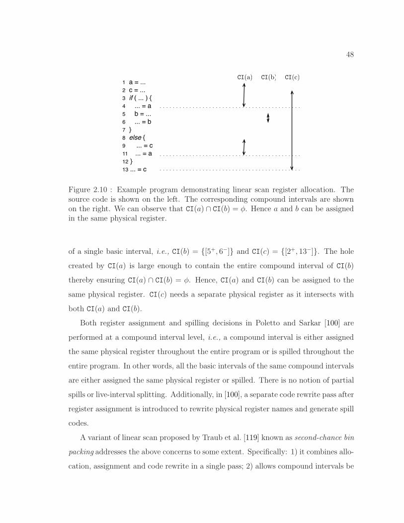
48
1 a = ...
2 c = ...
3 if ( ... ) {
4 ... = a
5 b = ...
6 ... = b
7 }
8 else {
9 ... = c
11 ... = a
12 }
13 ... = c
CI(b) CI(c)CI(a)
Figure 2.10 : Example program demonstrating linear scan register allocation. Thesource code is shown on the left. The corresponding compound intervals are shownon the right. We can observe that CI(a) ∩ CI(b) = φ. Hence a and b can be assignedin the same physical register.
of a single basic interval, i.e., CI(b) = {[5+, 6−]} and CI(c) = {[2+, 13−]}. The hole
created by CI(a) is large enough to contain the entire compound interval of CI(b)
thereby ensuring CI(a) ∩ CI(b) = φ. Hence, CI(a) and CI(b) can be assigned to the
same physical register. CI(c) needs a separate physical register as it intersects with
both CI(a) and CI(b).
Both register assignment and spilling decisions in Poletto and Sarkar [100] are
performed at a compound interval level, i.e., a compound interval is either assigned
the same physical register throughout the entire program or is spilled throughout the
entire program. In other words, all the basic intervals of the same compound intervals
are either assigned the same physical register or spilled. There is no notion of partial
spills or live-interval splitting. Additionally, in [100], a separate code rewrite pass after
register assignment is introduced to rewrite physical register names and generate spill
codes.
A variant of linear scan proposed by Traub et al. [119] known as second-chance bin
packing addresses the above concerns to some extent. Specifically: 1) it combines allo-
cation, assignment and code rewrite in a single pass; 2) allows compound intervals be
49
split multiple times (i.e., a CI can be assigned to a physical register in some program
points and be assigned to a memory location in some other program points, giving
it a second chance for allocation). Their algorithm walks over the IR instructions
in a linear order. When a new CI is encountered, it rewrites the output code with
an available physical register. If no such physical register is available, it spills a CI
based on a next-use distance metric [14] and inserts spill code appropriately. When a
spilled CI is encountered later on, it tries to give a second chance to the CI by finding
an available physical register at the current program point. If an available physical
register is found and the current reference of CI is a read, a memory load instruction is
added. If the current reference is a write, then no memory store instruction is added
until some other CI evicts the physical register. Further memory store instructions
can be avoided during eviction of a CI that is held in a physical register r, if the value
held in r matches that of the memory location of CI5. Since CIs can be allocated
in multiple physical registers at various program points, control flow needs to be
accounted, i.e., appropriate load, store, and move instructions are added on control
flow edges for generating correct code. For example, if the same CI was spilled at the
source end of a control flow edge and was in a physical register at the destination end
of a control flow edges, then a memory load instruction is added along the control
flow edge.
As can be seen above, the second-chance binpacking algorithm [119] spends more
time in compilation as it makes repetitive decisions of spill or register assignment
at every reference of an interval. In comparison, Poletto and Sarkar [100] make
decisions of spill or register assignment at interval start points and it does not offer
opportunities for second-chance.
Like second chance binpacking, more recently Wimmer and Mossenbock [123]
present a linear scan algorithm for x86 architectures that allows splitting of live
5This requires a data-flow analysis to determine memory consistency and is performed beforeregister allocation.
50
intervals by allowing some part of the CI to be in a register and some other part be
in memory. Like memory store optimizations of [119], they allow split positions be
placed in low-frequency basic blocks.
One of the key observations made while comparing Linear Scan with Graph
Coloring is that Linear Scan should be used when compile-time space and time
overhead is at a premium (as in dynamic compilation), but an algorithm based on
graph coloring should be used when the best runtime performance is desired. Let us
discuss some of the key reasons why this is the case. One of the limitations of current
linear scan is that it combines allocation and assignment in a single pass for improved
compilation time. This leads to local decisions for allocations and assignments at a
given instruction or at an interval start point based on active list. Instead, the spilling
decisions of a graph coloring is global because the spilling decisions are made based on
the interference graph that represents a global view of program. The global decisions
usually yield improved spilling and register assignment.
Chapter 6 of this dissertation addresses the limitations of current linear scan
register allocation algorithms and presents a space-efficient register allocation algo-
rithm [105] that retains the compile-time efficiency of linear scan while delivering
performance that can match or surpass that of Graph Coloring. The proposed register
allocation algorithm performs allocation and assignment in a compile-time efficient
manner in two separate passes.
2.7.2.3 SSA-based Register Allocation
Recently, much of the attention in register allocation has shifted to performing register
allocation in SSA representation. The key property of a SSA program is that every
variable is defined exactly once. This leads to the fact that an interference graph
built from the live ranges of a SSA program is a chordal graph [22, 29, 59]. A graph
is chordal if every cycle with four or more edges has a chord, that is, an edge which is
not part of the cycle but which connects two vertices on the cycle. For example, the
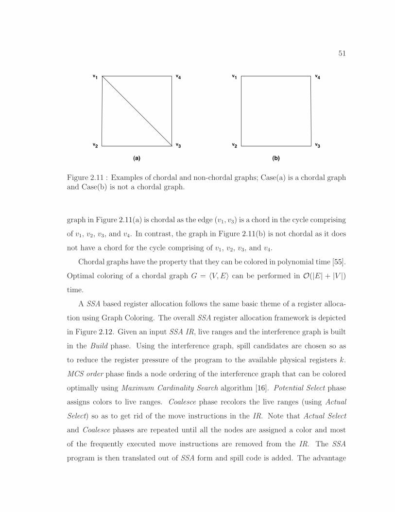
51
v1
v2 v3
v4 v1
v2 v3
v4
(a) (b)
Figure 2.11 : Examples of chordal and non-chordal graphs; Case(a) is a chordal graphand Case(b) is not a chordal graph.
graph in Figure 2.11(a) is chordal as the edge (v1, v3) is a chord in the cycle comprising
of v1, v2, v3, and v4. In contrast, the graph in Figure 2.11(b) is not chordal as it does
not have a chord for the cycle comprising of v1, v2, v3, and v4.
Chordal graphs have the property that they can be colored in polynomial time [55].
Optimal coloring of a chordal graph G = 〈V, E〉 can be performed in O(|E| + |V |)time.
A SSA based register allocation follows the same basic theme of a register alloca-
tion using Graph Coloring. The overall SSA register allocation framework is depicted
in Figure 2.12. Given an input SSA IR, live ranges and the interference graph is built
in the Build phase. Using the interference graph, spill candidates are chosen so as
to reduce the register pressure of the program to the available physical registers k.
MCS order phase finds a node ordering of the interference graph that can be colored
optimally using Maximum Cardinality Search algorithm [16]. Potential Select phase
assigns colors to live ranges. Coalesce phase recolors the live ranges (using Actual
Select) so as to get rid of the move instructions in the IR. Note that Actual Select
and Coalesce phases are repeated until all the nodes are assigned a color and most
of the frequently executed move instructions are removed from the IR. The SSA
program is then translated out of SSA form and spill code is added. The advantage
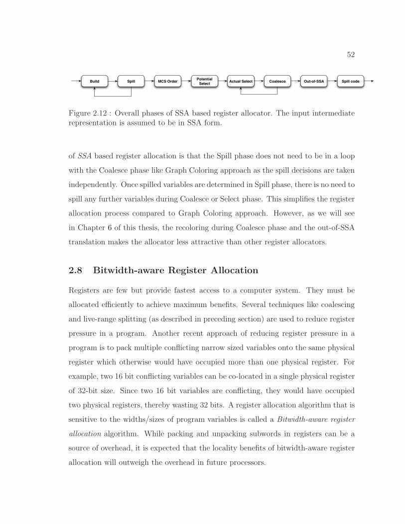
52
Build Spill MCS Order Actual Select Coalesce Out-of-SSA Spill codePotential
Select
Figure 2.12 : Overall phases of SSA based register allocator. The input intermediaterepresentation is assumed to be in SSA form.
of SSA based register allocation is that the Spill phase does not need to be in a loop
with the Coalesce phase like Graph Coloring approach as the spill decisions are taken
independently. Once spilled variables are determined in Spill phase, there is no need to
spill any further variables during Coalesce or Select phase. This simplifies the register
allocation process compared to Graph Coloring approach. However, as we will see
in Chapter 6 of this thesis, the recoloring during Coalesce phase and the out-of-SSA
translation makes the allocator less attractive than other register allocators.
2.8 Bitwidth-aware Register Allocation
Registers are few but provide fastest access to a computer system. They must be
allocated efficiently to achieve maximum benefits. Several techniques like coalescing
and live-range splitting (as described in preceding section) are used to reduce register
pressure in a program. Another recent approach of reducing register pressure in a
program is to pack multiple conflicting narrow sized variables onto the same physical
register which otherwise would have occupied more than one physical register. For
example, two 16 bit conflicting variables can be co-located in a single physical register
of 32-bit size. Since two 16 bit variables are conflicting, they would have occupied
two physical registers, thereby wasting 32 bits. A register allocation algorithm that is
sensitive to the widths/sizes of program variables is called a Bitwidth-aware register
allocation algorithm. While packing and unpacking subwords in registers can be a
source of overhead, it is expected that the locality benefits of bitwidth-aware register
allocation will outweigh the overhead in future processors.
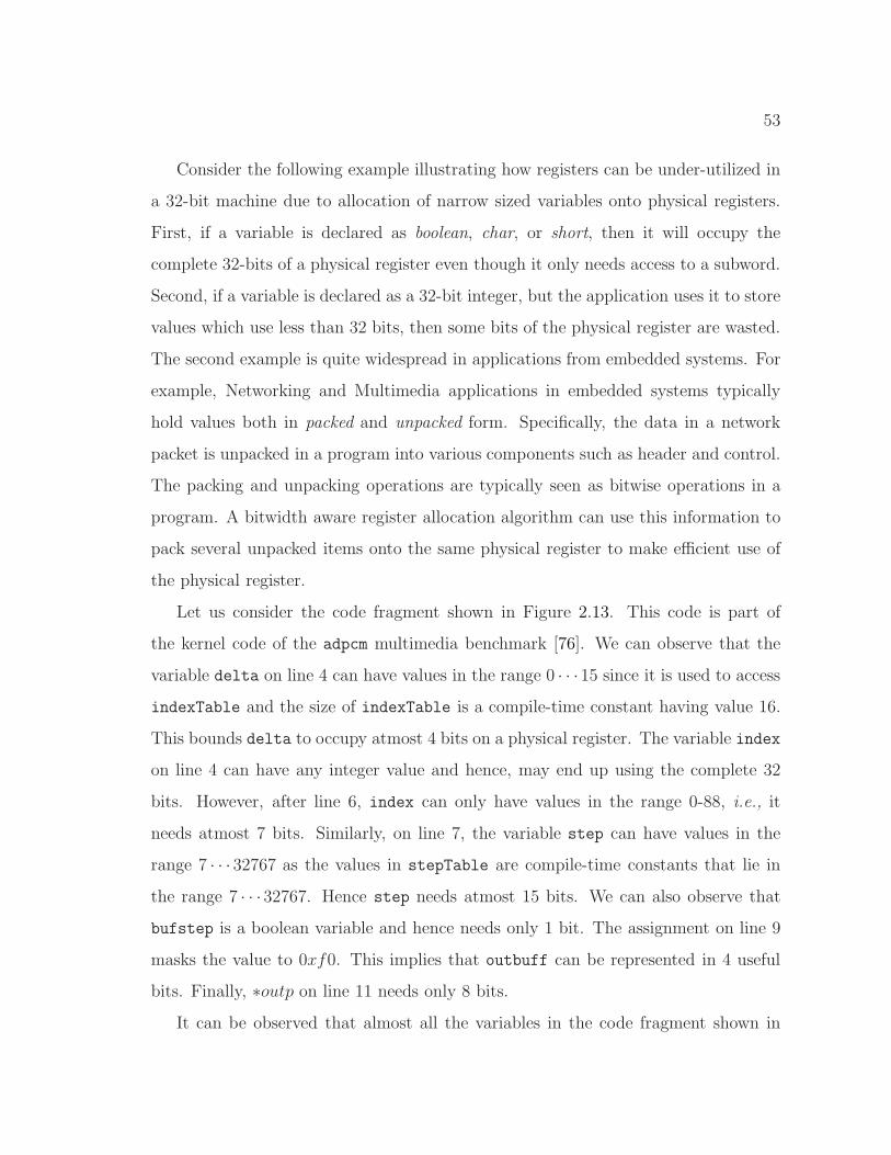
53
Consider the following example illustrating how registers can be under-utilized in
a 32-bit machine due to allocation of narrow sized variables onto physical registers.
First, if a variable is declared as boolean, char, or short, then it will occupy the
complete 32-bits of a physical register even though it only needs access to a subword.
Second, if a variable is declared as a 32-bit integer, but the application uses it to store
values which use less than 32 bits, then some bits of the physical register are wasted.
The second example is quite widespread in applications from embedded systems. For
example, Networking and Multimedia applications in embedded systems typically
hold values both in packed and unpacked form. Specifically, the data in a network
packet is unpacked in a program into various components such as header and control.
The packing and unpacking operations are typically seen as bitwise operations in a
program. A bitwidth aware register allocation algorithm can use this information to
pack several unpacked items onto the same physical register to make efficient use of
the physical register.
Let us consider the code fragment shown in Figure 2.13. This code is part of
the kernel code of the adpcm multimedia benchmark [76]. We can observe that the
variable delta on line 4 can have values in the range 0 · · ·15 since it is used to access
indexTable and the size of indexTable is a compile-time constant having value 16.
This bounds delta to occupy atmost 4 bits on a physical register. The variable index
on line 4 can have any integer value and hence, may end up using the complete 32
bits. However, after line 6, index can only have values in the range 0-88, i.e., it
needs atmost 7 bits. Similarly, on line 7, the variable step can have values in the
range 7 · · · 32767 as the values in stepTable are compile-time constants that lie in
the range 7 · · ·32767. Hence step needs atmost 15 bits. We can also observe that
bufstep is a boolean variable and hence needs only 1 bit. The assignment on line 9
masks the value to 0xf0. This implies that outbuff can be represented in 4 useful
bits. Finally, ∗outp on line 11 needs only 8 bits.
It can be observed that almost all the variables in the code fragment shown in
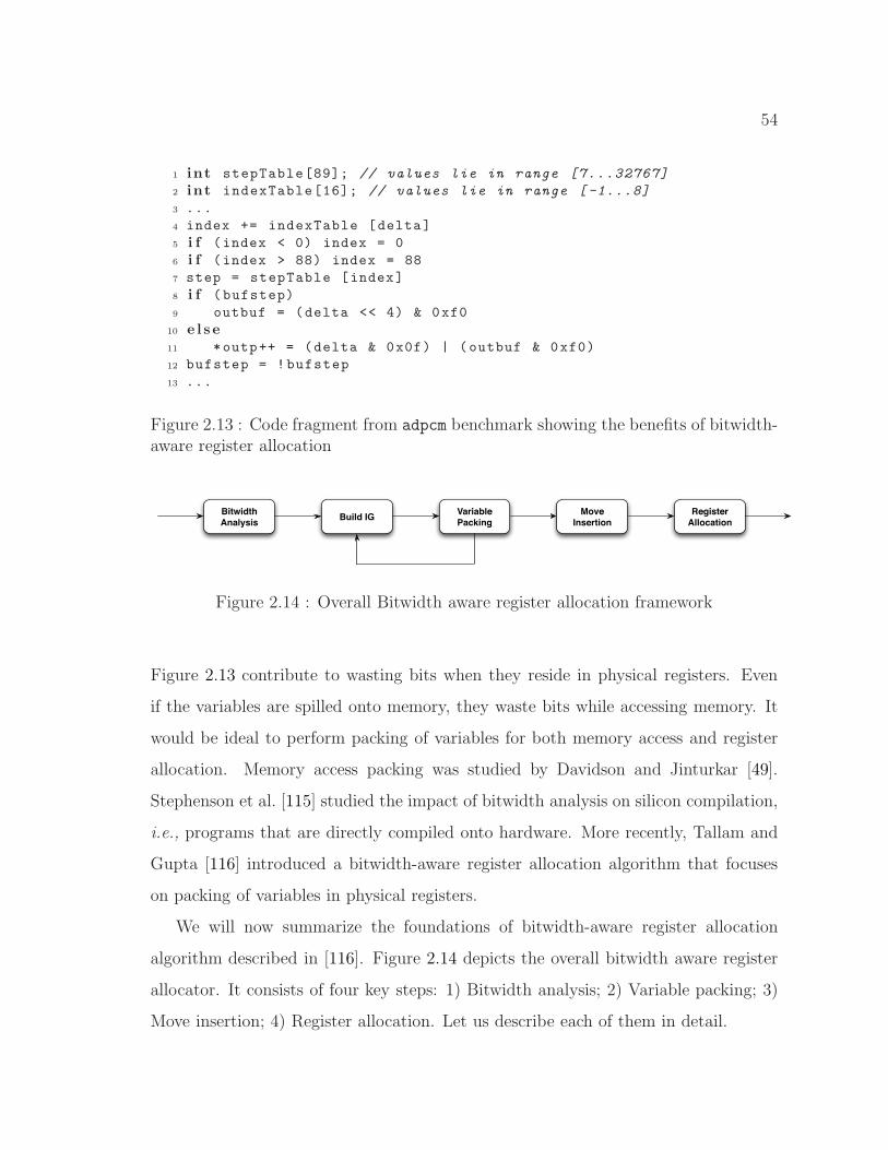
54
1 int stepTable[89]; // values lie in range [7...32767]
2 int indexTable[16]; // values lie in range [ -1...8]
3 ...
4 index += indexTable [delta]
5 i f (index < 0) index = 0
6 i f (index > 88) index = 88
7 step = stepTable [index]
8 i f (bufstep)
9 outbuf = (delta << 4) & 0xf0
10 e l s e
11 *outp++ = (delta & 0x0f) | (outbuf & 0xf0)
12 bufstep = !bufstep
13 ...
Figure 2.13 : Code fragment from adpcm benchmark showing the benefits of bitwidth-aware register allocation
Bitwidth
AnalysisBuild IG
Variable
Packing
Move
Insertion
Register
Allocation
Figure 2.14 : Overall Bitwidth aware register allocation framework
Figure 2.13 contribute to wasting bits when they reside in physical registers. Even
if the variables are spilled onto memory, they waste bits while accessing memory. It
would be ideal to perform packing of variables for both memory access and register
allocation. Memory access packing was studied by Davidson and Jinturkar [49].
Stephenson et al. [115] studied the impact of bitwidth analysis on silicon compilation,
i.e., programs that are directly compiled onto hardware. More recently, Tallam and
Gupta [116] introduced a bitwidth-aware register allocation algorithm that focuses
on packing of variables in physical registers.
We will now summarize the foundations of bitwidth-aware register allocation
algorithm described in [116]. Figure 2.14 depicts the overall bitwidth aware register
allocator. It consists of four key steps: 1) Bitwidth analysis; 2) Variable packing; 3)
Move insertion; 4) Register allocation. Let us describe each of them in detail.
55
2.8.1 Bitwidth Analysis
Bitwidth analysis is a static analysis that determines the actual widths (or bits)
of variables at various program points. We denote the width of a variable v at a
program point p as B(v, p). Before we describe how to compute B(v, p) information,
it is necessary to have a representation for B(v, p). There exists two representations
in the literature: 1) value range based representation proposed by Stephenson et
al. [115] that determines minimum and maximum value assigned to a variable; 2)
dead bit representation proposed by Tallam and Gupta [116] that divides the width
of a variable into three contiguous sections: (a) leading dead bits representing the bits
having zeros in the leading part when the variable is represented in binary; (b) middle
live bits representing the actual bit used; (c) trailing dead bits representing the bits
having zeros in the trailing part. Even though the value range based representation
is more precise, the dead bit representation is better suited for use by the register
allocator. The dead bit representation can be stated formally as:
Definition 2.8.1 The width of a variable v at program point p is a pair of leading
and trailing dead bits, i.e., B(v, p) = (l(v, p), t(v, p)), where l(v, p) denotes the size of
leading dead bits and t(v, p) denotes the size of trailing dead bits when v is represented
in binary.
Now let us discuss how bitwidth information B(v, p) for variables are computed.
The definition points of variables in the program generate new width information
that needs to be propagated to their uses. This involves a forward data flow analysis
that propagates bitwidth information along control flow edges on a lattice over all
possible pairs of (l(v, p), t(v, p)) with merge functions that take appropriate max or
min actions. Further, the type of usage of a variable at a program point (arising
from bitwise operations like shifting, masking, or-ing) can improve the precision of
the forward data flow analysis. These new bitwidth information need to be propagated
back from use program points to the definition program points using a backward data
56
flow analysis. Using both the forward and backward data flow algorithms, B(v, p) for
every variable at every program point is computed.
2.8.2 Variable Packing
Variable packing is the process of packing multiple variables onto the same physical
register. We would like to distinguish between the terms coalescing and packing
which are sometimes used inconsistently in the literature. Coalescing (as described
in Section 2.7.1.3) attempts to combine two non-interfering variables so as to remove
any move instruction between them. In contrast, packing attempts to combine two
interfering variables that can fit onto the same physical registers. Packing is shown
to be an NP-complete problem by Tallam and Gupta [116] using a simple reduction
from bin-packing.
Packing is usually performed on an interference graph whose interfering edges
are annotated with bitwidth information between two variables having maximum
width. The maximum width is represented using maximum interference width (MIW).
Formally,
Definition 2.8.2 MIW(v1, v2) = |B(v1, p)| + |B(v2, p)| such that ∄n, |B(v1, n)| +
|B(v2, n)| > |B(v1, p)|+ |B(v2, p)|, where |B(v, p)| denotes the middle section of useful
bits in dead bit representation.
Initially, each interfering edge between v1 and v2 is annotated with (|B(v1, n)|,|B(v2, n)|)where n is the program point having maximum interference width. The packing algo-
rithm proceeds by packing variables in the interference graph as long as MIW(v1, v2)
is less than the size of a physical register. One subtlety that occurs while packing is
that every step of packing needs recomputation of MIW as new packed variables are
formed. This can be an expensive operation as it needs to walk over the IR every time.
Tallam and Gupta[116] proposed the use of estimates of MIW (known as estimated
maximum interference width, i.e., EMIW) that are conservative approximation of
MIW and can be computed in constant time without traversing the IR.
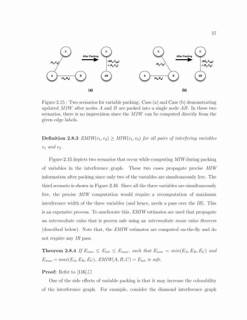
57
A B
C
(Ab,Ba)
(Ac,Ca)
A B
C
(Ab,Ba)
(Bc,Cb)
AB
C
(ABc,Cab)
= (Ac,Ca)
After Packing After Packing
AB
C
(ABc,Cab)
= (Bc,Cb)
(a) (b)
Figure 2.15 : Two scenarios for variable packing: Case (a) and Case (b) demonstratingupdated MIW after nodes A and B are packed into a single node AB. In these twoscenarios, there is no imprecision since the MIW can be computed directly from thegiven edge labels.
Definition 2.8.3 EMIW(v1, v2) ≥ MIW(v1, v2) for all pairs of interfering variables
v1 and v2.
Figure 2.15 depicts two scenarios that occur while computing MIW during packing
of variables in the interference graph. These two cases propagate precise MIW
information after packing since only two of the variables are simultaneously live. The
third scenario is shown in Figure 2.16. Since all the three variables are simultaneously
live, the precise MIW computation would require a recomputation of maximum
interference width of the three variables (and hence, needs a pass over the IR). This
is an expensive process. To ameliorate this, EMIW estimates are used that propagate
an intermediate value that is proven safe using an intermediate mean value theorem
(described below). Note that, the EMIW estimates are computed on-the-fly and do
not require any IR pass.
Theorem 2.8.4 If Emin ≤ Eint ≤ Emax, such that Emin = min(EA, EB, EC) and
Emax = max(EA, EB, EC), EMIW(A, B, C) = Eint is safe.
Proof: Refer to [116].�
One of the side effects of variable packing is that it may increase the colorability
of the interference graph. For example, consider the diamond interference graph
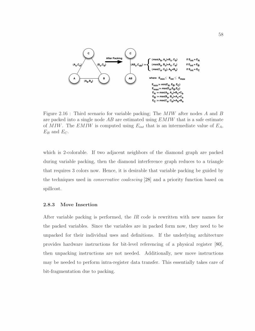
58
A B
C
(Ab,Ba)
(Ac,Ca)
AB
C
(ABc,Cab) :=
After Packing
(Bc,Cb)
(max(Ab, Ac)+Bc, Cb) if Eint = EA
(max(Ba, Bc)+Ac, Ca) if Eint = EB
(max(Ca, Cb), Ab+Ba) if Eint = EC
{where Emin Eint Emax ≤ ≤
Emin:= min(EA, EB, EC)
Emax:= max(EA,EB,EC)
EA := max(Ab, Ac)+Bc+CbEB := max(Ba, Bc)+Ac+CaEC := max(Ca, Cb)+Ab+Ba
Figure 2.16 : Third scenario for variable packing; The MIW after nodes A and Bare packed into a single node AB are estimated using EMIW that is a safe estimateof MIW . The EMIW is computed using Eint that is an intermediate value of EA,EB and EC .
which is 2-colorable. If two adjacent neighbors of the diamond graph are packed
during variable packing, then the diamond interference graph reduces to a triangle
that requires 3 colors now. Hence, it is desirable that variable packing be guided by
the techniques used in conservative coalescing [28] and a priority function based on
spillcost.
2.8.3 Move Insertion
After variable packing is performed, the IR code is rewritten with new names for
the packed variables. Since the variables are in packed form now, they need to be
unpacked for their individual uses and definitions. If the underlying architecture
provides hardware instructions for bit-level referencing of a physical register [80],
then unpacking instructions are not needed. Additionally, new move instructions
may be needed to perform intra-register data transfer. This essentially takes care of
bit-fragmentation due to packing.
59
2.8.4 Register Allocation
The final step of bitwidth aware register allocation algorithm is to perform register
allocation of the packed variables. Since the code was rewritten in the Move Insertion
phase, the interference graph needs to be rebuilt and a standard Graph Coloring
register allocation is performed.
Chapter 7 of this dissertation makes several contributions [11] to the bitwidth-
aware register allocation. First, it proposes a limit study on bitwidth analysis that
indicates the opportunities available for improving the bitwidth aware register alloca-
tor. Second, it proposes several enhancements to bitwidth analysis that closes the gap
between runtime bitwidth analysis and static bitwidth analysis. Finally, it proposes a
number of EMIW estimates that enhances the precision of variable packing compared
to Tallam-Gupta variable packing.
60
Chapter 3
May-Happen-in-Parallel (MHP) Analysis
In this chapter, we describe a May-Happen-in-Parallel (MHP) analysis for HJ pro-
grams that determines if two statements can execute in parallel. As described in
Section 2.2, HJ is a modern object-oriented programming language designed for high
performance and high productivity programming of parallel and multi-core computer
systems. HJ offers various concurrency control constructs to the programmers: mul-
tiple parallel activities can be created using the async construct, their termination
can be coordinated using the finish construct, mutual exclusion can be enforced
using isolated blocks, and barrier based synchronization among activities can be
performed using the phaser construct [107]. HJ also inherits from X10 the partitioning
of data and activities across places through the use of distributions. In this chapter
we describe a MHP analysis for HJ programs that consists of the async, finish,
isolated, and place constructs.
3.1 Introduction
May-Happen-in-Parallel (MHP) analysis statically determines if it is possible for
execution instances of two given statements (or the same statement) to execute in
parallel. This analysis serves as foundations for static analysis of concurrent programs
and debugging tools for a concurrent program [39, 71, 87, 91]. Static analysis
techniques that may benefit from MHP analysis include detection of synchronization
anomalies like data-races and deadlock, and improving the accuracy of compiler
analysis by removing infeasible def-use pairs.
Several MHP analyses have been proposed in the literature, e.g., [10, 92]. However,
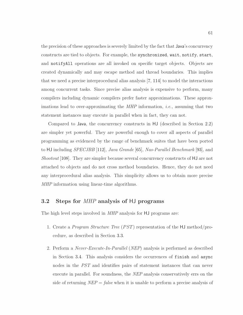
61
the precision of these approaches is severely limited by the fact that Java’s concurrency
constructs are tied to objects. For example, the synchronized, wait, notify, start,
and notifyAll operations are all invoked on specific target objects. Objects are
created dynamically and may escape method and thread boundaries. This implies
that we need a precise interprocedural alias analysis [7, 114] to model the interactions
among concurrent tasks. Since precise alias analysis is expensive to perform, many
compilers including dynamic compilers prefer faster approximations. These approx-
imations lead to over-approximating the MHP information, i.e., assuming that two
statement instances may execute in parallel when in fact, they can not.
Compared to Java, the concurrency constructs in HJ (described in Section 2.2)
are simpler yet powerful. They are powerful enough to cover all aspects of parallel
programming as evidenced by the range of benchmark suites that have been ported
to HJ including SPECJBB [112], Java Grande [65], Nas-Parallel Benchmark [93], and
Shootout [108]. They are simpler because several concurrency constructs of HJ are not
attached to objects and do not cross method boundaries. Hence, they do not need
any interprocedural alias analysis. This simplicity allows us to obtain more precise
MHP information using linear-time algorithms.
3.2 Steps for MHP analysis of HJ programs
The high level steps involved in MHP analysis for HJ programs are:
1. Create a Program Structure Tree (PST ) representation of the HJ method/pro-
cedure, as described in Section 3.3.
2. Perform a Never-Execute-In-Parallel (NEP) analysis is performed as described
in Section 3.4. This analysis considers the occurrences of finish and async
nodes in the PST and identifies pairs of statement instances that can never
execute in parallel. For soundness, the NEP analysis conservatively errs on the
side of returning NEP = false when it is unable to perform a precise analysis of
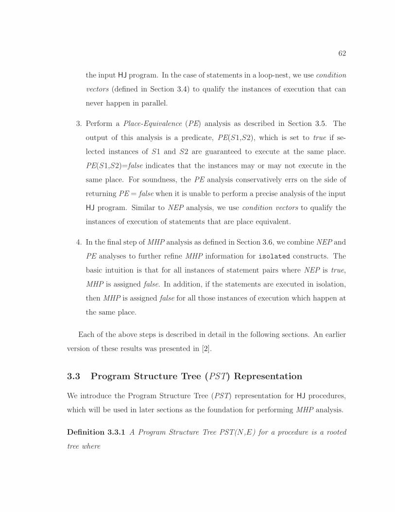
62
the input HJ program. In the case of statements in a loop-nest, we use condition
vectors (defined in Section 3.4) to qualify the instances of execution that can
never happen in parallel.
3. Perform a Place-Equivalence (PE) analysis as described in Section 3.5. The
output of this analysis is a predicate, PE(S1,S2), which is set to true if se-
lected instances of S1 and S2 are guaranteed to execute at the same place.
PE(S1,S2)=false indicates that the instances may or may not execute in the
same place. For soundness, the PE analysis conservatively errs on the side of
returning PE = false when it is unable to perform a precise analysis of the input
HJ program. Similar to NEP analysis, we use condition vectors to qualify the
instances of execution of statements that are place equivalent.
4. In the final step of MHP analysis as defined in Section 3.6, we combine NEP and
PE analyses to further refine MHP information for isolated constructs. The
basic intuition is that for all instances of statement pairs where NEP is true,
MHP is assigned false. In addition, if the statements are executed in isolation,
then MHP is assigned false for all those instances of execution which happen at
the same place.
Each of the above steps is described in detail in the following sections. An earlier
version of these results was presented in [2].
3.3 Program Structure Tree (PST) Representation
We introduce the Program Structure Tree (PST) representation for HJ procedures,
which will be used in later sections as the foundation for performing MHP analysis.
Definition 3.3.1 A Program Structure Tree PST(N ,E) for a procedure is a rooted
tree where
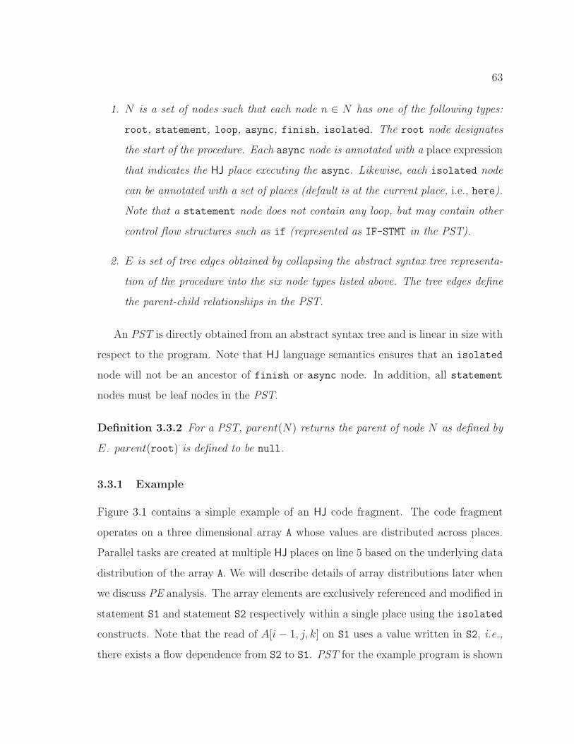
63
1. N is a set of nodes such that each node n ∈ N has one of the following types:
root, statement, loop, async, finish, isolated. The root node designates
the start of the procedure. Each async node is annotated with a place expression
that indicates the HJ place executing the async. Likewise, each isolated node
can be annotated with a set of places (default is at the current place, i.e., here).
Note that a statement node does not contain any loop, but may contain other
control flow structures such as if (represented as IF-STMT in the PST).
2. E is set of tree edges obtained by collapsing the abstract syntax tree representa-
tion of the procedure into the six node types listed above. The tree edges define
the parent-child relationships in the PST.
An PST is directly obtained from an abstract syntax tree and is linear in size with
respect to the program. Note that HJ language semantics ensures that an isolated
node will not be an ancestor of finish or async node. In addition, all statement
nodes must be leaf nodes in the PST.
Definition 3.3.2 For a PST, parent(N) returns the parent of node N as defined by
E. parent(root) is defined to be null.
3.3.1 Example
Figure 3.1 contains a simple example of an HJ code fragment. The code fragment
operates on a three dimensional array A whose values are distributed across places.
Parallel tasks are created at multiple HJ places on line 5 based on the underlying data
distribution of the array A. We will describe details of array distributions later when
we discuss PE analysis. The array elements are exclusively referenced and modified in
statement S1 and statement S2 respectively within a single place using the isolated
constructs. Note that the read of A[i − 1, j, k] on S1 uses a value written in S2, i.e.,
there exists a flow dependence from S2 to S1. PST for the example program is shown
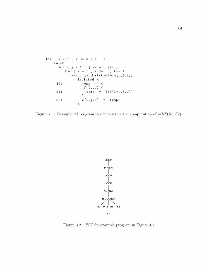
64
for ( i = 1 ; i <= n ; i++ )
f i n i s h
for ( j = 1 ; j <= n ; j++ )
for ( k = 1 ; k <= n ; k++ )
async (A.distr ibut ion[i,j,k])
i so lated {
S0: temp = 0;
i f (...) {
S1: temp = f(A[i-1,j,k]);
}
S2: A[i,j,k] = temp;
}
Figure 3.1 : Example HJ program to demonstrate the computation of MHP(S1, S2).
LOOP
FINISH
LOOP
LOOP
ASYNC
ISOLATED
S0 IF-STMT
S1
S2
Figure 3.2 : PST for example program in Figure 3.1
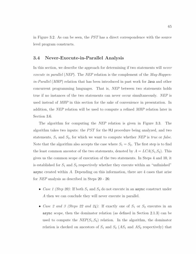
65
in Figure 3.2. As can be seen, the PST has a direct correspondence with the source
level program constructs.
3.4 Never-Execute-in-Parallel Analysis
In this section, we describe the approach for determining if two statements will never
execute in parallel (NEP). The NEP relation is the complement of the May-Happen-
in-Parallel (MHP) relation that has been introduced in past work for Java and other
concurrent programming languages. That is, NEP between two statements holds
true if no instances of the two statements can never occur simultaneously. NEP is
used instead of MHP in this section for the sake of convenience in presentation. In
addition, the NEP relation will be used to compute a refined MHP relation later in
Section 3.6.
The algorithm for computing the NEP relation is given in Figure 3.3. The
algorithm takes two inputs: the PST for the HJ procedure being analyzed, and two
statements, S1 and S2, for which we want to compute whether NEP is true or false.
Note that the algorithm also accepts the case where S1 = S2. The first step is to find
the least common ancestor of the two statements, denoted by A = LCA(S1,S2). This
gives us the common scope of execution of the two statements. In Steps 4 and 10, it
is established for S1 and S2 respectively whether they execute within an “unfinished”
async created within A. Depending on this information, there are 4 cases that arise
for NEP analysis as described in Steps 20 - 26:
• Case 1 (Step 20): If both S1 and S2 do not execute in an async construct under
A then we can conclude they will never execute in parallel.
• Case 2 and 3 (Steps 22 and 24): If exactly one of S1 or S2 executes in an
async scope, then the dominator relation (as defined in Section 2.1.3) can be
used to compute the NEP(S1,S2) relation. In the algorithm, the dominator
relation is checked on ancestors of S1 and S2 (AS1 and AS2 respectively) that
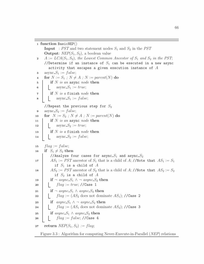
66
function BasicNEP()1
Input : PST and two statement nodes S1 and S2 in the PSTOutput: NEP(S1, S2), a boolean valueA := LCA(S1, S2), the Lowest Common Ancestor of S1 and S2 in the PST;2
//Determine if an instance of S1 can be executed in a new async
activity that escapes a given execution instance of Aasync S1 := false;3
for N := S1 ; N 6= A ; N := parent(N) do4
if N is an async node then5
async S1 := true;6
if N is a finish node then7
async S1 := false;8
//Repeat the previous step for S2
async S2 := false;9
for N := S2 ; N 6= A ; N := parent(N) do10
if N is an async node then11
async S2 := true;12
if N is a finish node then13
async S2 := false;14
flag := false;15
if S1 6= S2 then16
//Analyze four cases for async S1 and async S2
AS1 := PST ancestor of S1 that is a child of A; //Note that AS1 := S117
if S1 is a child of AAS2 := PST ancestor of S2 that is a child of A; //Note that AS2 := S218
if S2 is a child of Aif ¬ async S1 ∧ ¬ async S2 then19
flag := true; //Case 120
if ¬ async S1 ∧ async S2 then21
flag := (AS2 does not dominate AS1); //Case 222
if async S1 ∧ ¬ async S2 then23
flag := (AS1 does not dominate AS2); //Case 324
if async S1 ∧ async S2 then25
flag := false; //Case 426
return NEP(S1, S2) := flag;27
Figure 3.3 : Algorithm for computing Never-Execute-in-Parallel (NEP) relations
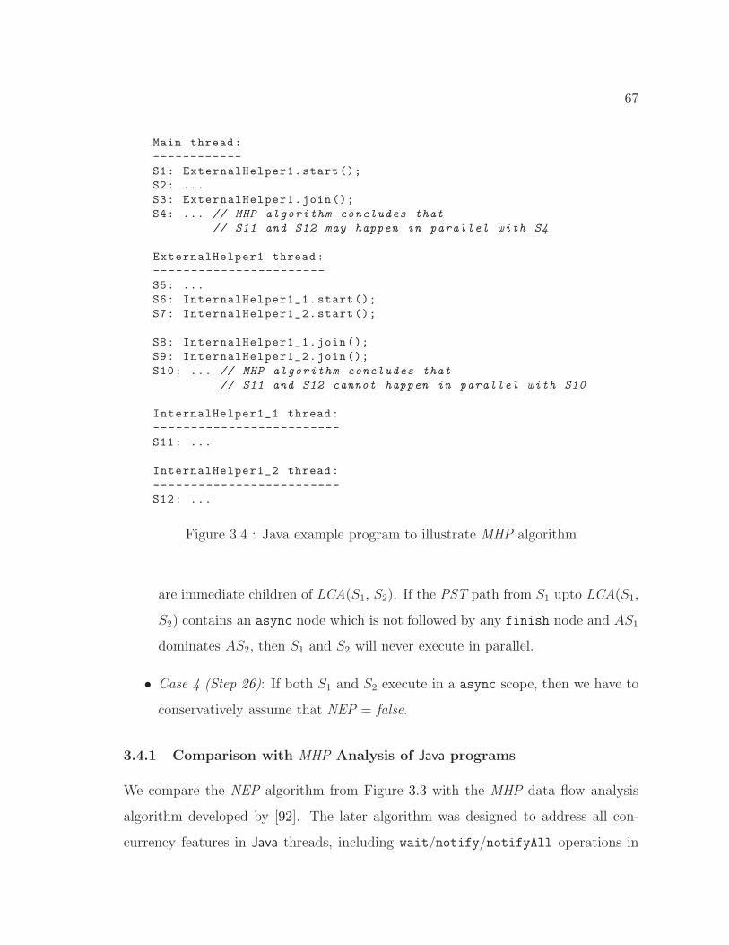
67
Main thread:
------------
S1: ExternalHelper1.start ();
S2: ...
S3: ExternalHelper1.join();
S4: ... // MHP algorithm concludes that
// S11 and S12 may happen in parallel with S4
ExternalHelper1 thread:
-----------------------
S5: ...
S6: InternalHelper1_1.start();
S7: InternalHelper1_2.start();
S8: InternalHelper1_1.join();
S9: InternalHelper1_2.join();
S10: ... // MHP algorithm concludes that
// S11 and S12 cannot happen in parallel with S10
InternalHelper1_1 thread:
-------------------------
S11: ...
InternalHelper1_2 thread:
-------------------------
S12: ...
Figure 3.4 : Java example program to illustrate MHP algorithm
are immediate children of LCA(S1, S2). If the PST path from S1 upto LCA(S1,
S2) contains an async node which is not followed by any finish node and AS1
dominates AS2, then S1 and S2 will never execute in parallel.
• Case 4 (Step 26): If both S1 and S2 execute in a async scope, then we have to
conservatively assume that NEP = false.
3.4.1 Comparison with MHP Analysis of Java programs
We compare the NEP algorithm from Figure 3.3 with the MHP data flow analysis
algorithm developed by [92]. The later algorithm was designed to address all con-
currency features in Java threads, including wait/notify/notifyAll operations in
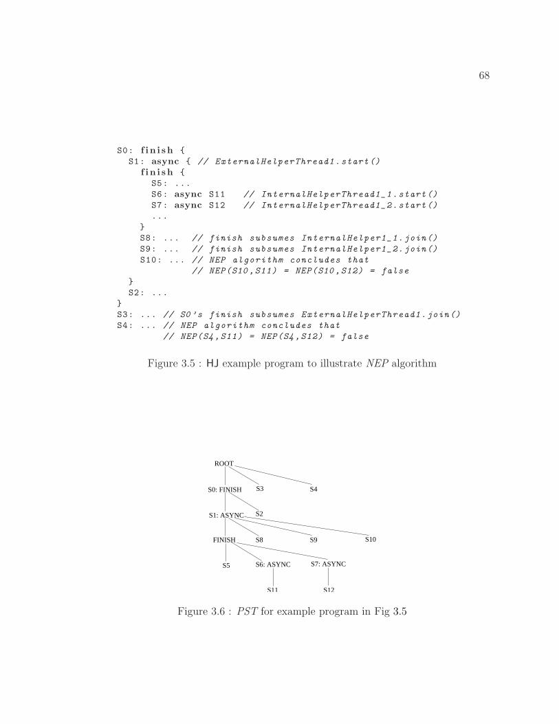
68
S0: f i n i s h {
S1: async { // ExternalHelperThread1.start()
f i n i s h {
S5: ...
S6: async S11 // InternalHelperThread1_1.start()
S7: async S12 // InternalHelperThread1_2.start()
...
}
S8: ... // finish subsumes InternalHelper1_1.join()
S9: ... // finish subsumes InternalHelper1_2.join()
S10: ... // NEP algorithm concludes that
// NEP(S10 ,S11) = NEP(S10 ,S12) = false
}
S2: ...
}
S3: ... // S0 ’s finish subsumes ExternalHelperThread1.join()
S4: ... // NEP algorithm concludes that
// NEP(S4,S11) = NEP(S4 ,S12) = false
Figure 3.5 : HJ example program to illustrate NEP algorithm
ROOT
S0: FINISH
S1: ASYNC
FINISH
S5 S6: ASYNC S7: ASYNC
S3 S4
S2
S8 S9 S10
S11 S12
Figure 3.6 : PST for example program in Fig 3.5
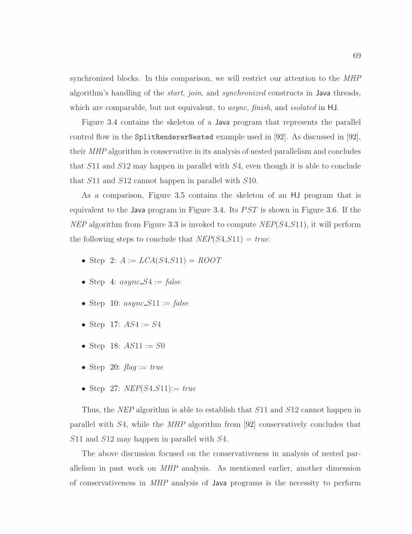
69
synchronized blocks. In this comparison, we will restrict our attention to the MHP
algorithm’s handling of the start, join, and synchronized constructs in Java threads,
which are comparable, but not equivalent, to async, finish, and isolated in HJ.
Figure 3.4 contains the skeleton of a Java program that represents the parallel
control flow in the SplitRendererNested example used in [92]. As discussed in [92],
their MHP algorithm is conservative in its analysis of nested parallelism and concludes
that S11 and S12 may happen in parallel with S4, even though it is able to conclude
that S11 and S12 cannot happen in parallel with S10.
As a comparison, Figure 3.5 contains the skeleton of an HJ program that is
equivalent to the Java program in Figure 3.4. Its PST is shown in Figure 3.6. If the
NEP algorithm from Figure 3.3 is invoked to compute NEP(S4,S11), it will perform
the following steps to conclude that NEP(S4,S11) = true:
• Step 2: A := LCA(S4,S11) = ROOT
• Step 4: async S4 := false
• Step 10: async S11 := false
• Step 17: AS4 := S4
• Step 18: AS11 := S0
• Step 20: flag := true
• Step 27: NEP(S4,S11):= true
Thus, the NEP algorithm is able to establish that S11 and S12 cannot happen in
parallel with S4, while the MHP algorithm from [92] conservatively concludes that
S11 and S12 may happen in parallel with S4.
The above discussion focused on the conservativeness in analysis of nested par-
allelism in past work on MHP analysis. As mentioned earlier, another dimension
of conservativeness in MHP analysis of Java programs is the necessity to perform
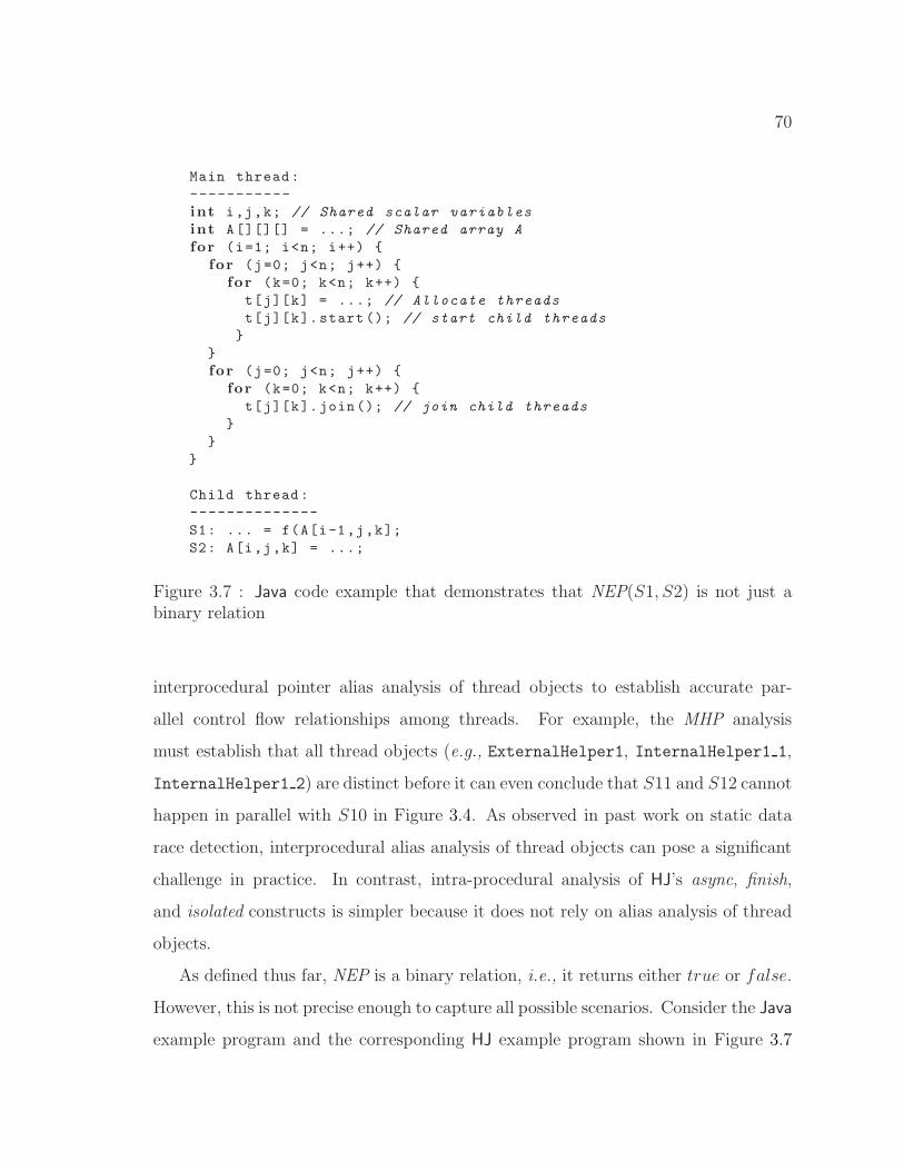
70
Main thread:
-----------
int i,j,k; // Shared scalar variables
int A[][][] = ...; // Shared array A
for (i=1; i<n; i++) {
for (j=0; j<n; j++) {
for (k=0; k<n; k++) {
t[j][k] = ...; // Allocate threads
t[j][k].start (); // start child threads
}
}
for (j=0; j<n; j++) {
for (k=0; k<n; k++) {
t[j][k].join(); // join child threads
}
}
}
Child thread:
--------------
S1: ... = f(A[i-1,j,k];
S2: A[i,j,k] = ...;
Figure 3.7 : Java code example that demonstrates that NEP(S1, S2) is not just abinary relation
interprocedural pointer alias analysis of thread objects to establish accurate par-
allel control flow relationships among threads. For example, the MHP analysis
must establish that all thread objects (e.g., ExternalHelper1, InternalHelper1 1,
InternalHelper1 2) are distinct before it can even conclude that S11 and S12 cannot
happen in parallel with S10 in Figure 3.4. As observed in past work on static data
race detection, interprocedural alias analysis of thread objects can pose a significant
challenge in practice. In contrast, intra-procedural analysis of HJ’s async, finish,
and isolated constructs is simpler because it does not rely on alias analysis of thread
objects.
As defined thus far, NEP is a binary relation, i.e., it returns either true or false.
However, this is not precise enough to capture all possible scenarios. Consider the Java
example program and the corresponding HJ example program shown in Figure 3.7
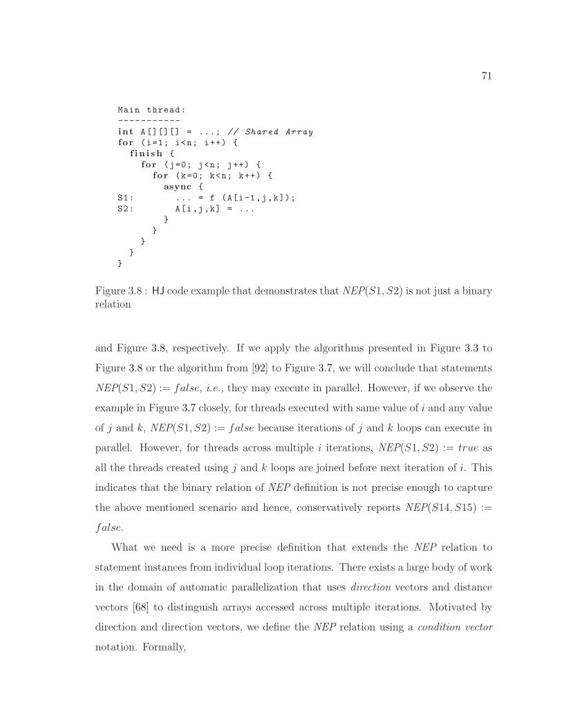
71
Main thread:
-----------
int A[][][] = ...; // Shared Array
for (i=1; i<n; i++) {
f i n i s h {
for (j=0; j<n; j++) {
for (k=0; k<n; k++) {
async {
S1: ... = f (A[i-1,j,k]);
S2: A[i,j,k] = ...
}
}
}
}
}
Figure 3.8 : HJ code example that demonstrates that NEP(S1, S2) is not just a binaryrelation
and Figure 3.8, respectively. If we apply the algorithms presented in Figure 3.3 to
Figure 3.8 or the algorithm from [92] to Figure 3.7, we will conclude that statements
NEP(S1, S2) := false, i.e., they may execute in parallel. However, if we observe the
example in Figure 3.7 closely, for threads executed with same value of i and any value
of j and k, NEP(S1, S2) := false because iterations of j and k loops can execute in
parallel. However, for threads across multiple i iterations, NEP(S1, S2) := true as
all the threads created using j and k loops are joined before next iteration of i. This
indicates that the binary relation of NEP definition is not precise enough to capture
the above mentioned scenario and hence, conservatively reports NEP(S14, S15) :=
false.
What we need is a more precise definition that extends the NEP relation to
statement instances from individual loop iterations. There exists a large body of work
in the domain of automatic parallelization that uses direction vectors and distance
vectors [68] to distinguish arrays accessed across multiple iterations. Motivated by
direction and direction vectors, we define the NEP relation using a condition vector
notation. Formally,
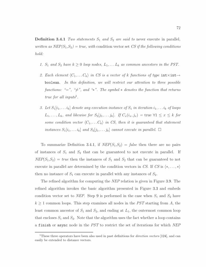
72
Definition 3.4.1 Two statements S1 and S2 are said to never execute in parallel,
written as NEP(S1,S2) = true, with condition vector set CS if the following conditions
hold:
1. S1 and S2 have k ≥ 0 loop nodes, L1, . . . Lk as common ancestors in the PST.
2. Each element 〈C1, . . . Ck〉 in CS is a vector of k functions of type int×int→boolean. In this definition, we will restrict our attention to three possible
functions: “=”, “ 6=”, and “∗”. The symbol ∗ denotes the function that returns
true for all inputs1.
3. Let S1[i1, . . . ik] denote any execution instance of S1 in iteration i1, . . . ik of loops
L1, . . . , Lk, and likewise for S2[j1, . . . jk]. If Cx(ix, jx) = true ∀1 ≤ x ≤ k for
some condition vector 〈C1, . . . Ck〉 in CS, then it is guaranteed that statement
instances S1[i1, . . . ik] and S2[j1, . . . jk] cannot execute in parallel. �
To summarize Definition 3.4.1, if NEP(S1,S2) = false then there are no pairs
of instances of S1 and S2 that can be guaranteed to not execute in parallel. If
NEP(S1,S2) = true then the instances of S1 and S2 that can be guaranteed to not
execute in parallel are determined by the condition vectors in CS. If CS is 〈∗, . . . , ∗〉then no instance of S1 can execute in parallel with any instances of S2.
The refined algorithm for computing the NEP relation is given in Figure 3.9. The
refined algorithm invokes the basic algorithm presented in Figure 3.3 and embeds
condition vector set to NEP. Step 9 is performed in the case when S1 and S2 have
k ≥ 1 common loops. This step examines all nodes in the PST starting from A, the
least common ancestor of S1 and S2, and ending at L1, the outermost common loop
that encloses S1 and S2. Note that the algorithm uses the fact whether a loop contains
a finish or async node in the PST to restrict the set of iterations for which NEP
1These three operators have been also used in past definitions for direction vectors [124], and caneasily be extended to distance vectors.
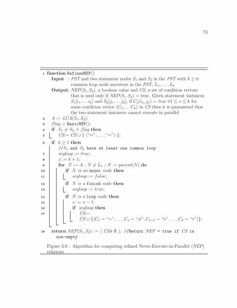
73
function RefinedNEP()1
Input : PST and two statement nodes S1 and S2 in the PST with k ≥ 0common loop node ancestors in the PST, L1, . . . , Lk
Output: NEP(S1, S2), a boolean value and CS, a set of condition vectorsthat is used only if NEP(S1, S2) = true. Given statement instancesS1[i1, . . . ik] and S2[j1, . . . jk], if Cx(ix, jx) = true ∀1 ≤ x ≤ k forsome condition vector 〈C1, . . . Ck〉 in CS then it is guaranteed thatthe two statement instances cannot execute in parallel
A := LCA(S1, S2);2
flag = BasicNEP();3
if S1 6= S2 ∧ flag then4
CS:= CS ∪ { 〈“=”, . . . , “=”〉 };5
if k ≥ 1 then6
//S1 and S2 have at least one common loop
seqloop := true;7
x := k + 1;8
for N := A ; N 6= L1 ; N := parent(N) do9
if N is an async node then10
seqloop := false;11
if N is a finish node then12
seqloop := true;13
if N is a loop node then14
x := x − 1;15
if seqloop then16
CS:=17
CS ∪ {〈C1 = “=”, . . . , Cx = “ 6=”, Cx+1 = “∗”, . . . , Ck = “∗”〉};
return NEP(S1, S2) := ( CS6= ∅ ); //Return NEP = true if CS is18
non-empty
Figure 3.9 : Algorithm for computing refined Never-Execute-in-Parallel (NEP)relations
74
= true. If (say) loop Lx contains a finish node that is an ancestor of both S1 and
S2 statements and there is no intervening async node in PST path from the finish
node to Lx, we observe that instances of S1 and S2 from two distinct iterations of Lx
(but created in the same iteration of outer loops L1, . . . , Lx−1) can never execute in
parallel. This property is captured by a condition vector in which Cx is set to “ 6=”,
C1, . . . , Cx−1 are set to “=”, and Cx+1, . . . , Ck are set to “∗”.
3.4.2 Complexity
The algorithm in Figure 3.9 assumes that the PST has already been constructed,
which is a one-time O(N) cost. In addition, Steps 22 and 24 of Figure 3.3 use the
dominator relation on the original control flow graph, which can be computed using
algorithms that vary in execution time complexity from O(NlogN), O(Nα(N)) [79]
to O(N) [61] as a one-time cost. We observe that the NEP algorithm takes O(H)
time to determine if a given pair of nodes, S1 and S2, satisfy NEP(S1,S2) = true,
where H is the height of the PST. Note that the condition vector set CS, can contain
at most L+1 condition vectors — one contributed by Step 5 and L by Step 17 – each
of which has O(L) size, where L ≤ H is the maximum nesting of loops in the PST.
Step 14 can be considered a constant time operation. If used to compute the NEP
relation for all pairs of statements, the total execution time will be O(N2H), which
is more efficient than the O(N3) time of the MHP algorithm in [92]. However, we
expect that the execution time overhead of the NEP algorithm will be much smaller
than O(N2H) in practice, since it can be used in a demand-driven fashion to only
compute the NEP relation for pairs of statements that are of interest to an interactive
tool or compiler transformation system.
3.4.3 Example
We start by using the example program in Figure 3.1 to illustrate the algorithm. The
example was intentionally chosen to be as simple as possible to illustrate the core
75
ideas. In this example, we are interested in determining which pairs of execution
instances of statements S1 and S2 will never execute in parallel with each other, so
the algorithm in Figure 3.9 will be invoked to compute NEP(S1,S2). The output of
this algorithm will be NEP(S1,S2) = true, with condition vector set CS= {〈 =, =, =
〉, 〈 6=, ∗, ∗〉}. This implies that two instances of S1 and S2 are guaranteed to never
execute in parallel if: 1) they belong to the same i-j-k iteration, or 2) they come
from iterations with distinct values of i. The first case is true because the statements
are executed in order with respect to the same async. The second case is true because
of the finish construct within each for-i loop iteration.
Now, let us use the following HJ code fragment to illustrate the four cases in
Step 15 in the basic NEP algorithm provided in Figure 3.3:
{ S1 ; async S2 ; S3 ; async S4 ; }
Case 1 NEP(S1, S3) = true, in accordance with Step 20.
Case 2 NEP(S1, S2) = true, in accordance with Step 22.
Case 3 NEP(S2, S3) = false, in accordance with Step 24.
Case 4 NEP(S2, S4) = false, in accordance with Step 26.
To summarize, the significant differences between the NEP analysis presented in
this chapter and past work on MHP analysis are as follows:
1. The availability of basic concurrency control constructs in HJ such as async and
finish enables a more efficient and precise NEP analysis algorithm compared
to past work on MHP analysis for Java. Our algorithm is based on simple path
traversals in the PST.
2. Past work on MHP analysis resulted in a simple true/false value for a given
pair of statements. Our work makes the NEP relation more precise by adding
76
condition vectors that are able to identify execution instances for which the
NEP relations hold.
3. As discussed later in Section 3.6, we show how the NEP information can be
further refined by using the isolation properties of isolated blocks in HJ.
3.5 Place Equivalence Analysis
In an attempt to combine shared-memory programming (e.g., Java, OpenMP, pthreads)
and distributed-memory programming (e.g., MPI, UPC), HJ inherits the place feature
from X10. Places co-locate data objects and the activities that operate on them.
This feature can also be used to mitigate some of the false-sharing issues that arise
in parallel computing. The activities that execute within a single place can have mu-
tually exclusive accesses using isolated HJ constructs. Before we analyze isolated
constructs, we need to determine if two statements can execute within the same place
or not.
In this section, we describe our approach for determining if two statements are
place equivalent (PE), i.e., if they will definitely execute at the same place. Most
parallel programming models that are currently used for distributed-memory mul-
tiprocessors follow a Single Program Multiple Data (SPMD) model in which one
thread is executed per place. However, the HJ programming model is more general
since it integrates thread-level parallelism and cluster-level parallelism by allowing
multiple activities to be created within the same place and across different places.
Place equivalence analysis therefore becomes important for more general parallel
programming models such as HJ.
Similar to the NEP relation, we need to distinguish the PE relation within loop
iterations using a condition vector set.
Definition 3.5.1 Two statements S1 and S2 are said to be place equivalent, written
as PE(S1, S2) = true, with condition vector set CS if the following conditions hold:
77
1. S1 and S2 have k ≥ 0 loop nodes, L1, . . . Lk as common ancestors in the PST
2. Let S1[i1, . . . ik] denote any execution instance of S1 in iteration i1, . . . ik of loops
L1, . . . , Lk, and likewise for S2[j1, . . . jk]. If Cx(ix, jx) = true ∀1 ≤ x ≤ k for
some condition vector 〈C1, . . . Ck〉 in CS, then it is guaranteed that statement
instances S1[i1, . . . ik] and S2[j1, . . . jk] must execute at the same place. �
To summarize Definition 3.5.1, if PE(S1,S2) = false then there are no pairs of
instance of S1 and S2 for which place equivalence is guaranteed. If PE(S1,S2) = true
then the instances of S1 and S2 that can be guaranteed to execute at the same place
are determined by the condition vectors in CS.
Before we describe the complete algorithm for PE computation, let us describe
two subtle issues that complicate the analysis. First, async statements in HJ can
be provided with an additional place expression to indicate the location/place of the
activity (without any place expression, the activity is created at the default place i.e.,
0). This implies that, given two statements S1 and S2, PE(S1, S2) needs to determine
if the place expression of the activity executing S1 is equal to the place expression
of the activity executing S2. This boils down to determining if two expressions can
have the same value. The idea is to perform a Definitely Same (as described in 2.6.1)
equivalence analysis, DS, on all place expressions in the procedure. For two place-
valued expressions, e1 and e2, DS(e1, e2) = true indicates that they must evaluate
to the same place. A global value numbering technique such as [6] can be used to
assign each expression e a value number V(e). DS can then be computed by using
the lexical identity, DS(e1, e2) := (V(e1) = V(e2)). More advanced techniques for
place equivalence analysis are described in [3, 37].
Second, the distributions of the underlying arrays accessed within a loop are
needed to determine place equivalence. Consider the following code fragment as
an example:
78
for ( i = 1 ; i < = n ; i++) // L1
for ( j = 1 ; j < = n ; j++) // L2
for ( k = 1 ; k < = n ; k++) // L3
async (A.distr ibut ion[f(i,j),k]) S;
We need to know the data distribution of array A in the async statement in
A.distribution[f(i,j),k]. In HJ and X10 [38], array A can be distributed using
a wide range of standard and user-defined distributions such as UNIQUE, RANDOM,
CYCLIC, and BLOCK. As an example, let us assume that A is distributed in (BLOCK,
∗) fashion so that A[m, ∗] is guaranteed to reside at the same place, where m is the
index of the first dimension. A depiction of (BLOCK, ∗) is shown in Figure 3.10. In this
figure, both (BLOCK, ∗) and (CYCLIC, ∗) will result in the same distribution because A
has p ∗ p elements. The async activity in the above code fragment with distribution
(BLOCK,∗) will be mapped to different places based on indices i and j, but not k,
i.e., place-variant with respect to loops L1 and L2. We term this kind of analysis
as LoopSet analysis. LoopSet determines loops for which a place expression is place
variant. The LoopSet for the above code fragment is LoopSet(A.distribution[f(i,j),k])
:= {L1,L2}, where L3 is not in the LoopSet indicates that it is place invariant.
LoopSet analysis for other HJ distributions can be determined in a similar fashion
to (BLOCK, ∗) and have been omitted for simplicity of presentation. Note that, it may
be in general hard to perform LoopSet analysis e.g., use of advanced features like
array views, and array projection. In such cases, we can always use a conservative
approach to include a loop in the LoopSet.
The algorithm for computing the PE relation is given in Figure 3.11. As described
above, the algorithm needs two additional pre-passes as inputs along with the PST.
First, a global place-value numbering pre-pass for place expressions to determine
place local information for statements. Second, a global loop-invariant analysis based
LoopSet analysis pre-pass to determine loops for which a given place expression is place
variant. Global value numbering can be performed using an SSA-based algorithm as
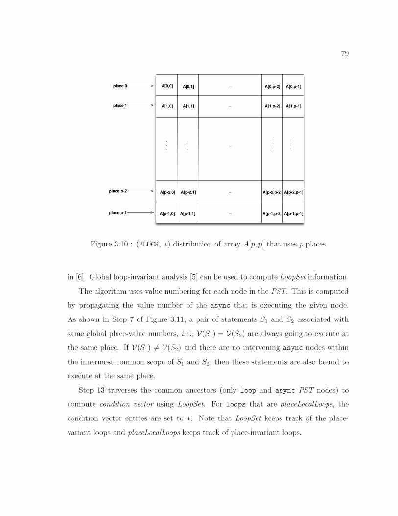
79
A[0,0] A[0,1] A[0,p-2] A[0,p-1]
A[1,0] A[1,1] A[1,p-2] A[1,p-1]
A[p-2,0] A[p-2,1] A[p-2,p-2] A[p-2,p-1]
A[p-1,0] A[p-1,1] A[p-1,p-2] A[p-1,p-1]...
...
...
...
...
.
.
.
.
.
.
.
.
.
.
.
.
place 0
place 1
place p-2
place p-1
Figure 3.10 : (BLOCK, ∗) distribution of array A[p, p] that uses p places
in [6]. Global loop-invariant analysis [5] can be used to compute LoopSet information.
The algorithm uses value numbering for each node in the PST. This is computed
by propagating the value number of the async that is executing the given node.
As shown in Step 7 of Figure 3.11, a pair of statements S1 and S2 associated with
same global place-value numbers, i.e., V(S1) = V(S2) are always going to execute at
the same place. If V(S1) 6= V(S2) and there are no intervening async nodes within
the innermost common scope of S1 and S2, then these statements are also bound to
execute at the same place.
Step 13 traverses the common ancestors (only loop and async PST nodes) to
compute condition vector using LoopSet. For loops that are placeLocalLoops, the
condition vector entries are set to ∗. Note that LoopSet keeps track of the place-
variant loops and placeLocalLoops keeps track of place-invariant loops.
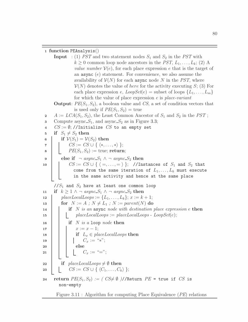
80
function PEAnalysis()1
Input : (1) PST and two statement nodes S1 and S2 in the PST withk ≥ 0 common loop node ancestors in the PST, L1, . . . , Lk; (2) Avalue number V(e), for each place expression e that is the target ofan async (e) statement. For convenience, we also assume theavailability of V(N) for each async node N in the PST, whereV(N) denotes the value of here for the activity executing S; (3) Foreach place expression e, LoopSet(e) = subset of loops {L1, . . . , Lm}for which the value of place expression e is place-variant
Output: PE(S1, S2), a boolean value and CS, a set of condition vectors thatis used only if PE(S1, S2) = true
A := LCA(S1, S2), the Least Common Ancestor of S1 and S2 in the PST ;2
Compute async S1, and async S2 as in Figure 3.3;3
CS := ∅; //Initialize CS to an empty set4
if S1 6= S2 then5
if V(S1) = V(S2) then6
CS := CS ∪ { 〈∗, . . . , ∗〉 };7
PE(S1, S2) := true; return;8
else if ¬ async S1 ∧ ¬ async S2 then9
CS := CS ∪ { 〈 =, . . . , = 〉 }; //Instances of S1 and S2 that10
come from the same iteration of L1, . . . , Lk must execute
in the same activity and hence at the same place
//S1 and S2 have at least one common loop
if k ≥ 1 ∧ ¬ async S1 ∧ ¬ async S2 then11
placeLocalLoops := {L1, . . . , Lk}; x := k + 1;12
for N := A ; N 6= L1 ; N := parent(N) do13
if N is an async node with destination place expression e then14
placeLocalLoops := placeLocalLoops - LoopSet(e);15
if N is a loop node then16
x := x − 1;17
if Lx ∈ placeLocalLoops then18
Cx := “∗”;19
else20
Cx := “=”;21
if placeLocalLoops 6= ∅ then22
CS := CS ∪ { 〈C1, . . . , Ck〉 };23
return PE(S1, S2) := ( CS 6= ∅ )//Return PE = true if CS is24
non-empty
Figure 3.11 : Algorithm for computing Place Equivalence (PE) relations
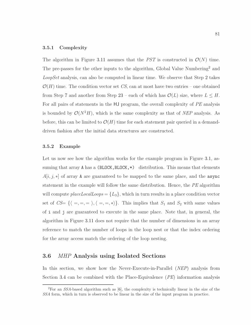
81
3.5.1 Complexity
The algorithm in Figure 3.11 assumes that the PST is constructed in O(N) time.
The pre-passes for the other inputs to the algorithm, Global Value Numbering2 and
LoopSet analysis, can also be computed in linear time. We observe that Step 2 takes
O(H) time. The condition vector set CS, can at most have two entries – one obtained
from Step 7 and another from Step 23 – each of which has O(L) size, where L ≤ H .
For all pairs of statements in the HJ program, the overall complexity of PE analysis
is bounded by O(N2H), which is the same complexity as that of NEP analysis. As
before, this can be limited to O(H) time for each statement pair queried in a demand-
driven fashion after the initial data structures are constructed.
3.5.2 Example
Let us now see how the algorithm works for the example program in Figure 3.1, as-
suming that array A has a (BLOCK,BLOCK,*) distribution. This means that elements
A[i, j, ∗] of array A are guaranteed to be mapped to the same place, and the async
statement in the example will follow the same distribution. Hence, the PE algorithm
will compute placeLocalLoops = {L3}, which in turn results in a place condition vector
set of CS= {〈 =, =, = 〉, 〈 =, =, ∗〉}. This implies that S1 and S2 with same values
of i and j are guaranteed to execute in the same place. Note that, in general, the
algorithm in Figure 3.11 does not require that the number of dimensions in an array
reference to match the number of loops in the loop nest or that the index ordering
for the array access match the ordering of the loop nesting.
3.6 MHP Analysis using Isolated Sections
In this section, we show how the Never-Execute-in-Parallel (NEP) analysis from
Section 3.4 can be combined with the Place-Equivalence (PE) information analysis
2For an SSA-based algorithm such as [6], the complexity is technically linear in the size of theSSA form, which in turn is observed to be linear in the size of the input program in practice.
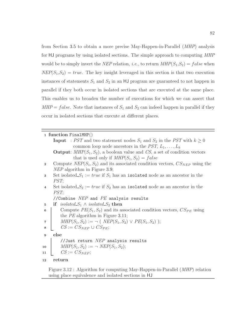
82
from Section 3.5 to obtain a more precise May-Happen-in-Parallel (MHP) analysis
for HJ programs by using isolated sections. The simple approach to computing MHP
would be to simply invert the NEP relation, i.e., to return MHP(S1,S2) = false when
NEP(S1,S2) = true. The key insight leveraged in this section is that two execution
instances of statements S1 and S2 in an HJ program are guaranteed to not happen in
parallel if they both occur in isolated sections that are executed at the same place.
This enables us to broaden the number of executions for which we can assert that
MHP = false. Note that instances of S1 and S2 can indeed happen in parallel if they
occur in isolated sections that execute at different places.
function FinalMHP()1
Input : PST and two statement nodes S1 and S2 in the PST with k ≥ 0common loop node ancestors in the PST, L1, . . . , Lk
Output: MHP(S1, S2), a boolean value and CS, a set of condition vectorsthat is used only if MHP(S1, S2) = false
Compute NEP(S1, S2) and its associated condition vectors, CSNEP using the2
NEP algorithm in Figure 3.9;Set isolated S1 := true if S1 has an isolated node as an ancestor in the3
PST;Set isolated S2 := true if S2 has an isolated node as an ancestor in the4
PST;//Combine NEP and PE analysis results
if isolated S1 ∧ isolated S2 then5
Compute PE(S1, S2) and its associated condition vectors, CSPE using6
the PE algorithm in Figure 3.11;MHP(S1, S2) := ¬ ( NEP(S1, S2) ∨ PE(S1, S2) );7
CS := CSNEP ∪ CSPE;8
else9
//Just return NEP analysis results
MHP(S1, S2) := ¬ NEP(S1, S2);10
CS := CSNEP ;11
return12
Figure 3.12 : Algorithm for computing May-Happen-in-Parallel (MHP) relationusing place equivalence and isolated sections in HJ
83
The algorithm for computing the MHP relation is given in Figure 3.12. For a
pair of statements S1 and S2, Steps 3 and 4 check if they are nested in isolated
blocks. In case both S1 and S2 are nested in isolated blocks, MHP(S1,S2) is computed
by combining the NEP and PE results in Step 7. Otherwise, the MHP relation is
computed directly from the NEP relation.
3.6.1 Complexity
The complexity of computing the MHP relation is bounded by O(N2H). This is due
to the complexity of computing both NEP relation and PE relation. As before, this
can be limited to O(H) time for each statement pair queried in a demand-driven
fashion after the initial data structures are constructed.
3.6.2 Example
As discussed earlier, the NEP solution computed using the analysis described in
Section 3.4 for the example in Figure 3.1 was NEP(S1,S2) = true with condition
vector set CSNEP = {〈 =, =, = 〉, 〈 6=, ∗, ∗〉}. This indicates that for different values
of loop index i, S1 and S2 can not execute in parallel. However, this information can
be refined using the PE solution due to the presence of isolated PST node in the
loop body. The PE solution computed using the analysis described in Section 3.5
was PE(S1,S2) = true with condition vector set CSPE = {〈 =, =, = 〉, 〈 =, =, ∗〉}.This indicates that S1 and S2 will execute at the same HJ place for different values
of loop index k but with same values for loop indices i and j. Using the above two
results, the algorithm in this section is able to determine that MHP(S1,S2) = false
with condition vector set CS = {〈 =, =, = 〉, 〈 6=, ∗, ∗〉, 〈 =, =, ∗〉}, i.e., MHP(S1,S2)
= false if they belong to the same i-j-k iteration, or if they come from iterations with
distinct values of i or with the same values of i and j.
84
3.7 Summary
In this chapter, we introduced a new demand-driven algorithm for May-Happen-
in-Parallel (MHP) analysis that is applicable to any language that adopts the core
concepts of places, async, finish, and isolated blocks from the HJ programming
model. The main contributions of this work compared to past MHP analysis algo-
rithms are as follows:
1. We introduced a more precise definition of the MHP relation than in pa st work
by adding condition vectors that identify execution instances for which the MHP
relation holds, instead of just returning a single true/false value for all pairs of
executing instances.
2. Compared to past work, the availability of basic concurrency control constructs
such as async and finish enabled the use of more efficient and precise analysis
algorithms based on simple path traversals in the Program Structure Tree, and
did not rely on interprocedural pointer alias analysis of thread objects as in
MHP analysis for the Java language.
3. We introduced place equivalence (PE) analysis to identify execution instances
that happen at the same place. The PE analysis helps us in leveraging the fact
that two statement instances which occur in isolated blocks that execute at the
same HJ place must have MHP = false.
MHP analysis described in this chapter can be extended in future to other ad-
vanced concurrency constructs of HJ such as future-force and phaser. Additionally,
the analysis currently operates at an intraprocedural level leaving extensions for
interprocedural level as future work [10], perhaps as extensions to the interprocedural
side effect analysis of parallel programs discussed in the next chapter.
85
Chapter 4
Side-Effect Analysis for Parallel Programs
Side-effect analysis determines the effects of a procedure call at a call site. Knowledge
of the side-effects of a procedure call has several important applications. For example,
many program analyses need to understand the effects of a procedure call so as to
enable program transformations across procedure boundaries. In Section 2.5, four
different types of side-effects using Banning’s formulation, i.e., MOD, REF, USE,
and DEF have been described. Both MOD and REF side-effects are flow-insensitive
problems where as USE and DEF are flow-sensitive problems. Flow-sensitive problems
are solved by tracing through control-flow paths where as flow-insensitive problems
are solved by ignoring the control flow paths. The complexity of computing MOD
side-effects using Banning’s approach (as described in Section 2.5) is O(NEα(E, N),
where E is the number of call sites in the program, N is the number of procedures in
the program and α represents the inverse Ackermanns’ function.
JIT and dynamic compilers perform program optimization and transformation
in limited situations. In particular they do not typically perform interprocedural
analyses. The reason behind this is two folds: 1) the whole program may not
be available during compilation and programs may be loaded dynamically; 2) the
complexity of interprocedural analyses is high. The former case is addressed by
closed-world solutions presented in [36]. This chapter addresses the later case and
presents a fast flow-insensitive and field-insensitive side-effect analysis. The side-
effect analysis does not need any interprocedural alias analysis to propagate the exact
object references modified or referenced. Instead, it unifies all the references of an
object field using a heap-array representation. This representation does not need any
86
special attention for parameter bindings.
Due to the advent of parallel programming languages for multi-core systems, the
analysis of parallel programs pose additional challenges to dynamic compilers due
to parallel constructs in the program. These parallel constructs in general carry
inherent side-effects in them and hence further add to the complexity of the side-
effect analysis. Note that there is a natural interplay between the side-effect analysis
and parallel constructs analysis, since parallel constructs are usually translated to low-
level runtime library procedure calls in the intermediate representation level at which
program transformations are performed. In this chapter, we propose an algorithm
to perform side-effect analysis of programs with parallel constructs in a dynamic
compiler.
Section 4.1 discusses a flow-insensitive and field-insensitive side-effect analysis
algorithm suitable for analyzing method calls in a dynamic compilation environment.
Section 4.2 describes how the side-effect analysis algorithm can be extended for the
async, finish, and isolated core parallel constructs of HJ programming language.
4.1 Side-Effect Analysis of Method Calls
Let us describe the impact of side-effect analysis on program transformations. Con-
sider the code fragment shown in Figure 4.1. Let us assume that we are performing
scalar replacement for load elimination transformation (as described in Section 2.6)
for method bar. We notice that there is a flow dependence from line 8 to line 10
indicating that the memory load on line 10 can be replaced by a scalar. However, the
load statement on line 10 cannot be scalar-replaced without the knowledge of the side-
effects of the method call setNothing() in line 9. In contrast, a scalar replacement for
load elimination algorithm based on interprocedural side-effect analysis can determine
that the method call setNothing() does not have any side-effects, thereby realizing
the opportunity for eliminating the load in line 10 by scalar replacing the value
assigned in line 8. We also observe that there is an input dependence from line 11
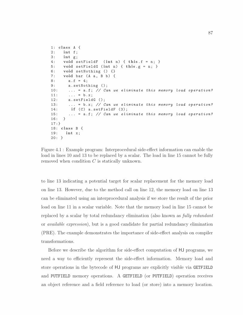
87
1: c l as s A {
2: int f;
3: int g;
4: void setFieldF ( int n) { th i s .f = n; }
5: void setFieldG ( int n) { th i s .g = n; }
6: void setNothing () {}
7: void bar (A a, B b) {
8: a.f = 4;
9: a.setNothing ();
10: ... = a.f; // Can we eliminate this memory load operation?
11: ... = b.x;
12: a.setFieldG ();
13: ... = b.x; // Can we eliminate this memory load operation?
14: i f (C) a.setFieldF (3);
15: ... = a.f; // Can we eliminate this memory load operation?
16: }
17:}
18: c l as s B {
19: int x;
20: }
Figure 4.1 : Example program: Interprocedural side-effect information can enable theload in lines 10 and 13 to be replaced by a scalar. The load in line 15 cannot be fullyremoved when condition C is statically unknown.
to line 13 indicating a potential target for scalar replacement for the memory load
on line 13. However, due to the method call on line 12, the memory load on line 13
can be eliminated using an interprocedural analysis if we store the result of the prior
load on line 11 in a scalar variable. Note that the memory load in line 15 cannot be
replaced by a scalar by total redundancy elimination (also known as fully redundant
or available expression), but is a good candidate for partial redundancy elimination
(PRE). The example demonstrates the importance of side-effect analysis on compiler
transformations.
Before we describe the algorithm for side-effect computation of HJ programs, we
need a way to efficiently represent the side-effect information. Memory load and
store operations in the bytecode of HJ programs are explicitly visible via GETFIELD
and PUTFIELD memory operations. A GETFIELD (or PUTFIELD) operation receives
an object reference and a field reference to load (or store) into a memory location.
88
We represent the field references using the heap array representation described in
Section 2.6.1.
4.1.1 Heap Array Representation
To recap from Section 2.6.1, each field x in the program is abstracted by a distinct
heap array, Hx. Hx represents all the instances of field x in the heap during runtime.
A GETFIELD of a.x is represented as an use of element Hx[a], and a PUTFIELD of b.x
is represented as a def of element Hx[b]. The use of heap arrays ensures that field x is
considered to be the same across instances of two different static types T1 and T2, if
(say) T1 is a subtype of T2. Heap arrays capture abstractions at the level of fields not
at the level of precise object references. Hence, they are field-insensitive. This level
of abstraction provides faster analysis in dynamic compilation as they avoid complex
interprocedural alias analysis for objects.
4.1.2 Method Level Side-effect
As discussed earlier, the goal of a side-effect analysis is to determine for each call
site, a safe approximation of the side-effects that the method involved at that call site
may have. This recursively includes any side effects of the methods called from that
site. We capture this using the generalized flow-insensitive side-effect formulation
proposed by Banning [9]. The generalized flow-insensitive side-effects of a method
are represented using GMOD and GREF sets. Using the heap array representation,
the AMOD, AREF, GMOD and GREF side-effects described in Section 2.5 can be
rewritten as:
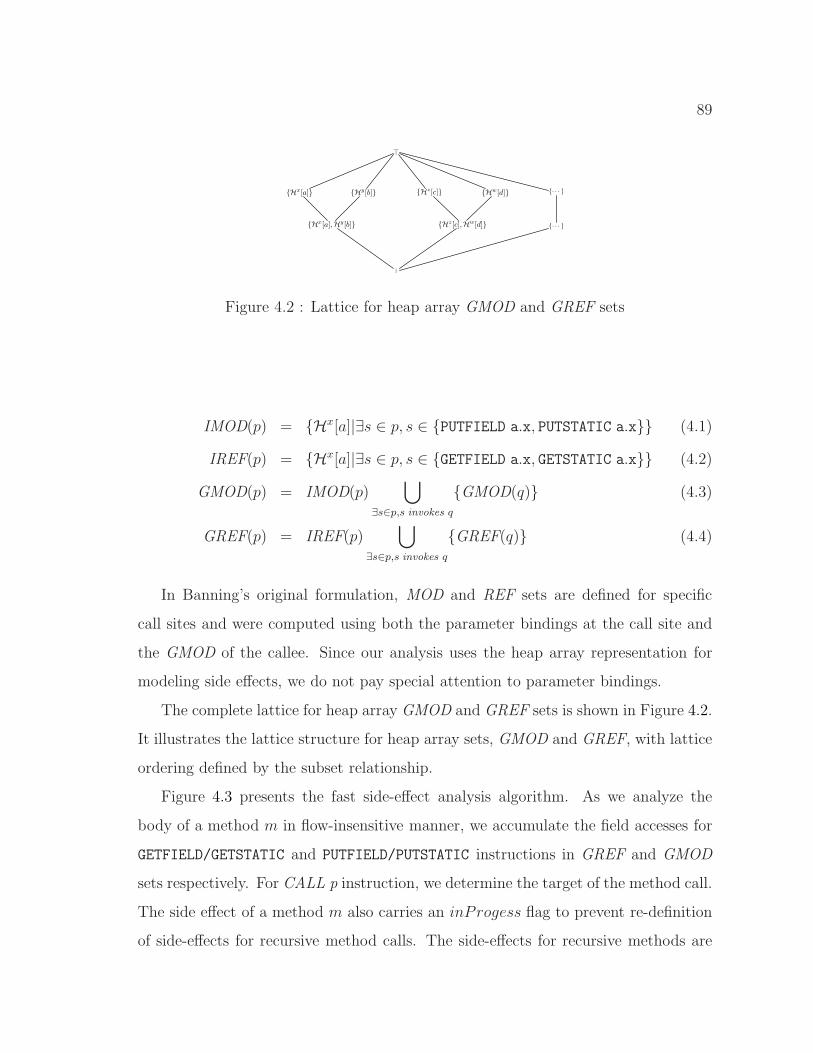
89
{Hx[a]} {Hy[b]} {Hz[c]} {Hw[d]} {· · · }
{Hx[a],Hy[b]} {Hz[c],Hw[d]} {· · · }
⊥
⊤
Figure 4.2 : Lattice for heap array GMOD and GREF sets
IMOD(p) = {Hx[a]|∃s ∈ p, s ∈ {PUTFIELD a.x, PUTSTATIC a.x}} (4.1)
IREF(p) = {Hx[a]|∃s ∈ p, s ∈ {GETFIELD a.x, GETSTATIC a.x}} (4.2)
GMOD(p) = IMOD(p)⋃
∃s∈p,s invokes q
{GMOD(q)} (4.3)
GREF(p) = IREF(p)⋃
∃s∈p,s invokes q
{GREF(q)} (4.4)
In Banning’s original formulation, MOD and REF sets are defined for specific
call sites and were computed using both the parameter bindings at the call site and
the GMOD of the callee. Since our analysis uses the heap array representation for
modeling side effects, we do not pay special attention to parameter bindings.
The complete lattice for heap array GMOD and GREF sets is shown in Figure 4.2.
It illustrates the lattice structure for heap array sets, GMOD and GREF, with lattice
ordering defined by the subset relationship.
Figure 4.3 presents the fast side-effect analysis algorithm. As we analyze the
body of a method m in flow-insensitive manner, we accumulate the field accesses for
GETFIELD/GETSTATIC and PUTFIELD/PUTSTATIC instructions in GREF and GMOD
sets respectively. For CALL p instruction, we determine the target of the method call.
The side effect of a method m also carries an inProgess flag to prevent re-definition
of side-effects for recursive method calls. The side-effects for recursive methods are
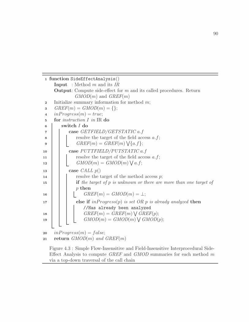
90
function SideEffectAnalysis()1
Input : Method m and its IROutput: Compute side-effect for m and its called procedures. Return
GMOD(m) and GREF(m)Initialize summary information for method m;2
GREF(m) = GMOD(m) = {};3
inProgress(m) = true;4
for instruction I in IR do5
switch I do6
case GETFIELD/GETSTATIC a.f7
resolve the target of the field access a.f ;8
GREF(m) = GREF(m)∨{a.f};9
case PUTTFIELD/PUTSTATIC a.f10
resolve the target of the field access a.f ;11
GMOD(m) = GMOD(m)∨
a.f ;12
case CALL p()13
resolve the target of the method access p;14
if the target of p is unknown or there are more than one target of15
p thenGREF(m) = GMOD(m) = ⊥;16
else if inProgress(p) is set OR p is already analyzed then17
//Has already been analyzed
GREF(m) = GREF(m)∨
GREF(p);18
GMOD(m) = GMOD(m)∨
GMOD(p);19
inProgress(m) = false;20
return GMOD(m) and GREF(m)21
Figure 4.3 : Simple Flow-Insensitive and Field-Insensitive Interprocedural Side-Effect Analysis to compute GREF and GMOD summaries for each method mvia a top-down traversal of the call chain
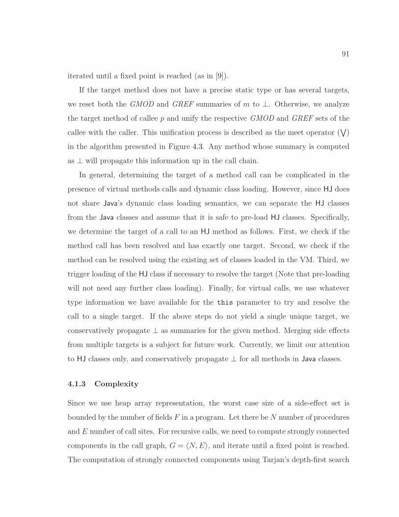
91
iterated until a fixed point is reached (as in [9]).
If the target method does not have a precise static type or has several targets,
we reset both the GMOD and GREF summaries of m to ⊥. Otherwise, we analyze
the target method of callee p and unify the respective GMOD and GREF sets of the
callee with the caller. This unification process is described as the meet operator (∨
)
in the algorithm presented in Figure 4.3. Any method whose summary is computed
as ⊥ will propagate this information up in the call chain.
In general, determining the target of a method call can be complicated in the
presence of virtual methods calls and dynamic class loading. However, since HJ does
not share Java’s dynamic class loading semantics, we can separate the HJ classes
from the Java classes and assume that it is safe to pre-load HJ classes. Specifically,
we determine the target of a call to an HJ method as follows. First, we check if the
method call has been resolved and has exactly one target. Second, we check if the
method can be resolved using the existing set of classes loaded in the VM. Third, we
trigger loading of the HJ class if necessary to resolve the target (Note that pre-loading
will not need any further class loading). Finally, for virtual calls, we use whatever
type information we have available for the this parameter to try and resolve the
call to a single target. If the above steps do not yield a single unique target, we
conservatively propagate ⊥ as summaries for the given method. Merging side effects
from multiple targets is a subject for future work. Currently, we limit our attention
to HJ classes only, and conservatively propagate ⊥ for all methods in Java classes.
4.1.3 Complexity
Since we use heap array representation, the worst case size of a side-effect set is
bounded by the number of fields F in a program. Let there be N number of procedures
and E number of call sites. For recursive calls, we need to compute strongly connected
components in the call graph, G = 〈N, E〉, and iterate until a fixed point is reached.
The computation of strongly connected components using Tarjan’s depth-first search
92
1: c l as s A {
2: int f;
3: void foo (A a) { a.f = n; }
4: void bar () {
5: A a = new A ();
6: A b = new A ();
7: a.f = 4;
8: foo (b);
9: ... = a.f; // Can we eliminate this load operation?
10: }
11:}
Figure 4.4 : Even with interprocedural side-effect information we can not ascertainthat the memory load on line 9 can be eliminated; We need an additional differently-different (DD) analysis to guarantee that a and b are guaranteed to be pointing todifferent objects in every execution of the program.
algorithm [117] is of O(N + E) complexity. Each step of the depth-first search
algorithm involves F field operations using a standard bit-vector implementation.
Thus the overall complexity of Algorithm 4.3 is O(N + E) ∗ F .
4.1.4 Discussion
Let us consider the example shown in Figure 4.4. Using Algorithm 4.3, GMOD(foo) =
{Hf [b]}. To scalar replace the memory load on line 9, i.e., heap array Hf [a], we need
to guarantee that a and b are pointing to different objects (in this case it is true as
a and b are assigned two different objects in lines 5 and 6 respectively). So we need
additional analysis to compute if two heap arrays are same or different that refines the
side-effect analysis results. The details of these analyses are provided in Section 2.6.3.
4.2 Extended Side-effect Analysis for Parallel Constructs
Consider the example HJ program shown in Figure 4.5, which will serve as a running
example to demonstrate side-effect analysis of parallel constructs in HJ programs.
The example program has a main method that invokes two asyncs (one in line 6 and
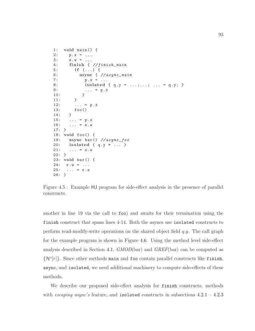
93
1: void main() {
2: p.x = ...
3: s.w = ...
4: f i n i s h { // finish_main
5: i f (...) {
6: async { // async_main
7: p.x = ...
8: i so lated { q.y = ...;...; ... = q.y; }
9: ... = p.x
10: }
11: }
12: ... = p.x
13: foo()
14: }
15: ... = p.x
16: ... = s.w
17: }
18: void foo() {
19: async bar() // async_foo
20: i so lated { q.y = ... }
21: ... = s.w
22: }
23: void bar() {
24: r.z = ...
25: ... = r.z
26: }
Figure 4.5 : Example HJ program for side-effect analysis in the presence of parallelconstructs.
another in line 19 via the call to foo) and awaits for their termination using the
finish construct that spans lines 4-14. Both the asyncs use isolated constructs to
perform read-modify-write operations on the shared object field q.y. The call graph
for the example program is shown in Figure 4.6. Using the method level side-effect
analysis described in Section 4.1, GMOD(bar) and GREF(bar) can be computed as
{Hz[r]}. Since other methods main and foo contain parallel constructs like finish,
async, and isolated, we need additional machinery to compute side-effects of these
methods.
We describe our proposed side-effect analysis for finish constructs, methods
with escaping async’s feature, and isolated constructs in subsections 4.2.1 – 4.2.3
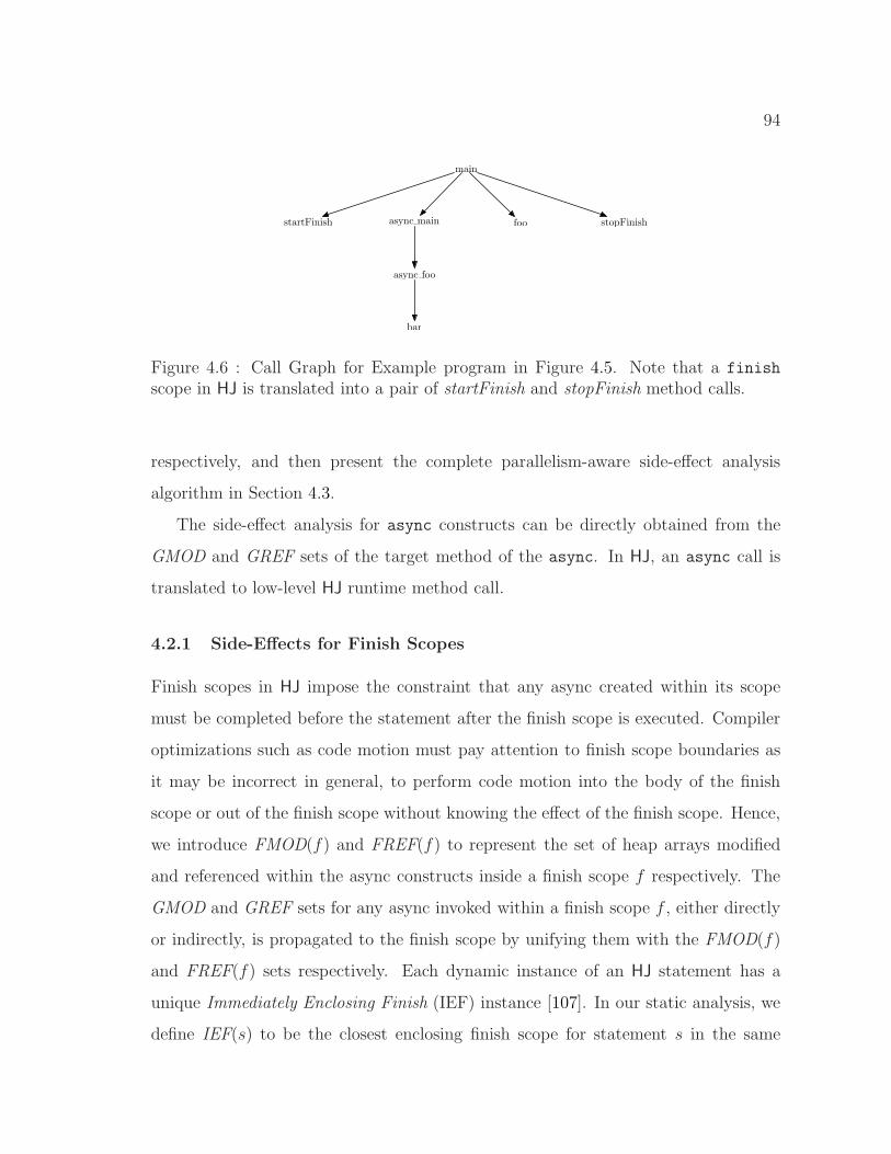
94
startFinish stopFinishasync main foo
main
async foo
bar
Figure 4.6 : Call Graph for Example program in Figure 4.5. Note that a finish
scope in HJ is translated into a pair of startFinish and stopFinish method calls.
respectively, and then present the complete parallelism-aware side-effect analysis
algorithm in Section 4.3.
The side-effect analysis for async constructs can be directly obtained from the
GMOD and GREF sets of the target method of the async. In HJ, an async call is
translated to low-level HJ runtime method call.
4.2.1 Side-Effects for Finish Scopes
Finish scopes in HJ impose the constraint that any async created within its scope
must be completed before the statement after the finish scope is executed. Compiler
optimizations such as code motion must pay attention to finish scope boundaries as
it may be incorrect in general, to perform code motion into the body of the finish
scope or out of the finish scope without knowing the effect of the finish scope. Hence,
we introduce FMOD(f) and FREF(f) to represent the set of heap arrays modified
and referenced within the async constructs inside a finish scope f respectively. The
GMOD and GREF sets for any async invoked within a finish scope f , either directly
or indirectly, is propagated to the finish scope by unifying them with the FMOD(f)
and FREF(f) sets respectively. Each dynamic instance of an HJ statement has a
unique Immediately Enclosing Finish (IEF) instance [107]. In our static analysis, we
define IEF(s) to be the closest enclosing finish scope for statement s in the same

95
method. IEF(s) is undefined, i.e., ⊥, if s does not have an enclosing finish statement
in the same method. We conservatively propagate ⊥ information for both FMOD
and FREF sets, when any method invoked inside a finish scope has unknown target
or multiple targets. Formally,
FMOD(f) =
⋃
∃s∈f,s invokes q{GMOD(q) ∪ EMOD(q)} if q is an async call⋃
∃s∈f,s invokes q{EMOD(q)} otherwise
FREF(f) =
⋃
∃s∈f,s invokes q{GREF(q) ∪ EREF(q)} if q is an async call⋃
∃s∈f,s invokes q{EREF(q)} otherwise
The async calls that are directly or indirectly (via other function calls) invoked
inside a finish scope f are captured in the FMOD and FREF. EMOD and EREF
capture MOD and REF sets for escaping asyncs described below.
Consider the method main in Example 4.5. The finish scope encompasses the
side-effects of all the methods and asyncs invoked within it. Ignoring the isolated
constructs on line 8 and 20 (which will be discussed later), the FMOD(finish main)
can be computed as {Hx[p],Hz[r]}. Hz[r] is added to the side-effect due to the
method call foo in the finish scope. Similarly, FREF(finish main) is computed as
{Hx[p],Hz[r],Hw[s]}.
4.2.2 Side-Effects for Methods with Escaping Asyncs
HJ permits methods with escaping asyncs, i.e., asyncs that have no enclosing finish
scopes in the same method. We define an async-escaping method as: 1) a method
which contains an async invocation that is not enclosed in a finish scope, or 2) a
method which invokes another async-escaping method that is not wrapped in a finish
scope. The GMOD and GREF sets for async-escaping methods are propagated to
their enclosing finish scopes as their termination is guaranteed only at the end of
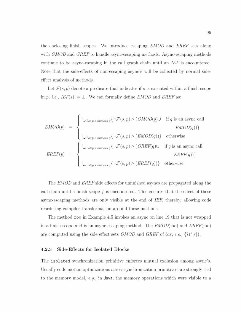
96
the enclosing finish scopes. We introduce escaping EMOD and EREF sets along
with GMOD and GREF to handle async-escaping methods. Async-escaping methods
continue to be async-escaping in the call graph chain until an IEF is encountered.
Note that the side-effects of non-escaping async’s will be collected by normal side-
effect analysis of methods.
Let F(s, p) denote a predicate that indicates if s is executed within a finish scope
in p, i.e., IEF(s)! = ⊥. We can formally define EMOD and EREF as:
EMOD(p) =
⋃
∃s∈p,s invokes q{¬F(s, p) ∧ (GMOD(q)∪ if q is an async call
EMOD(q))}⋃
∃s∈p,s invokes q{¬F(s, p) ∧ (EMOD(q))} otherwise
EREF(p) =
⋃
∃s∈p,s invokes q{¬F(s, p) ∧ (GREF(q)∪ if q is an async call
EREF(q))}⋃
∃s∈p,s invokes q{¬F(s, p) ∧ (EREF(q))} otherwise
The EMOD and EREF side effects for unfinished asyncs are propagated along the
call chain until a finish scope f is encountered. This ensures that the effect of these
async-escaping methods are only visible at the end of IEF, thereby, allowing code
reordering compiler transformation around these methods.
The method foo in Example 4.5 invokes an async on line 19 that is not wrapped
in a finish scope and is an async-escaping method. The EMOD(foo) and EREF(foo)
are computed using the side effect sets GMOD and GREF of bar, i.e., {Hz[r]}.
4.2.3 Side-Effects for Isolated Blocks
The isolated synchronization primitive enforces mutual exclusion among async’s.
Usually code motion optimizations across synchronization primitives are strongly tied
to the memory model, e.g., in Java, the memory operations which were visible to a
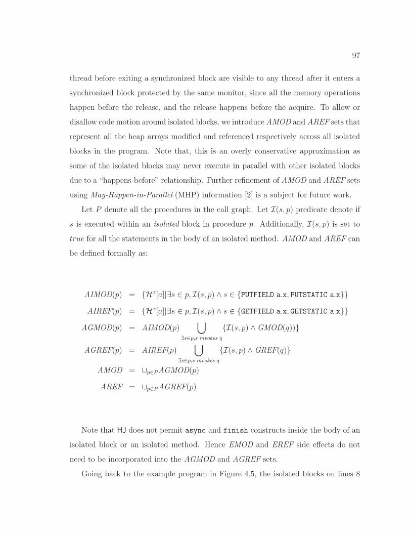
97
thread before exiting a synchronized block are visible to any thread after it enters a
synchronized block protected by the same monitor, since all the memory operations
happen before the release, and the release happens before the acquire. To allow or
disallow code motion around isolated blocks, we introduce AMOD and AREF sets that
represent all the heap arrays modified and referenced respectively across all isolated
blocks in the program. Note that, this is an overly conservative approximation as
some of the isolated blocks may never execute in parallel with other isolated blocks
due to a “happens-before” relationship. Further refinement of AMOD and AREF sets
using May-Happen-in-Parallel (MHP) information [2] is a subject for future work.
Let P denote all the procedures in the call graph. Let I(s, p) predicate denote if
s is executed within an isolated block in procedure p. Additionally, I(s, p) is set to
true for all the statements in the body of an isolated method. AMOD and AREF can
be defined formally as:
AIMOD(p) = {Hx[a]|∃s ∈ p, I(s, p) ∧ s ∈ {PUTFIELD a.x, PUTSTATIC a.x}}
AIREF(p) = {Hx[a]|∃s ∈ p, I(s, p) ∧ s ∈ {GETFIELD a.x, GETSTATIC a.x}}
AGMOD(p) = AIMOD(p)⋃
∃s∈p,s invokes q
{I(s, p) ∧ GMOD(q))}
AGREF(p) = AIREF(p)⋃
∃s∈p,s invokes q
{I(s, p) ∧ GREF(q)}
AMOD = ∪p∈PAGMOD(p)
AREF = ∪p∈PAGREF(p)
Note that HJ does not permit async and finish constructs inside the body of an
isolated block or an isolated method. Hence EMOD and EREF side effects do not
need to be incorporated into the AGMOD and AGREF sets.
Going back to the example program in Figure 4.5, the isolated blocks on lines 8
98
and 20 modify and reference heap array Hy[q]. Hence, AMOD = AREF = {Hy[q]}.
4.3 Parallelism-aware Side-Effect Analysis Algorithm
The overall side-effect analysis algorithm in the presence of finish, async, and
isolated constructs is presented in Figure 4.7. This algorithm is designed to be
performed on the Java bytecode performed by the HJ compiler, which translates each
async construct to a runAsync call in the Java-based HJ runtime, which in turn calls
the runHJTask method in an inner class that contains the body of the async.
Further, every finish scope is translated into a pair of startFinish() and stopFin-
ish() runtime calls.
For statements/methods executed in isolated blocks, we unify the AMOD and
AREF sets using the meet operator∨
i. The∨
i is a conditional meet operation
which is performed only if the current statement/method call is in an isolated block.
Note that the HJ language does not permit any usage of async or finish constructs
in the body of isolated sections [38].
The algorithm presented in Figure 4.7 walks over the IR in a flow-insensitive
manner and unifies the GMOD and GREF sets for heap arrays accessed in GETFIELD
(GETSTATIC) and PUTSTATIC (PUTFIELD) instructions respectively (as shown in steps 11
and 15). If these instructions are accessed within an isolated section, we unify
them with AMOD and AREF respectively (as shown in steps 12 and 16). For
Call p() instructions, we take different actions for different function calls due to
parallel constructs. For startFinish function call demarcating the start of a new finish
scope, we create, i.e., FMOD(IEF(I)) and FREF(IEF(I)) sets for the finish scope
(as shown in steps 7-10 in Figure 4.8). At stopFinish function call indicating activity
termination, FMOD(IEF(I)) and FREF(IEF(I)) are merged into the GMOD(m) and
GREF(m) sets for the current caller m (as shown in steps 12-15 in Figure 4.8). This
unification implies that the side-effect of the asyncs created within the finish scope
can only be visible at the end of the finish scope.
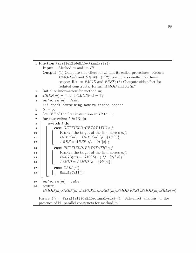
99
function ParallelSideEffectAnalysis()1
Input : Method m and its IROutput: (1) Compute side-effect for m and its called procedures: Return
GMOD(m) and GREF(m); (2) Compute side-effect for finishscopes: Return FMOD and FREF; (3) Compute side-effect forisolated constructs: Return AMOD and AREF
Initialize information for method m;2
GREF(m) = ⊤ and GMOD(m) = ⊤;3
inProgress(m) = true;4
//A stack containing active finish scopes
S := φ;5
Set IEF of the first instruction in IR to ⊥;6
for instruction I in IR do7
switch I do8
case GETFIELD/GETSTATIC a.f9
Resolve the target of the field access a.f ;10
GREF(m) = GREF(m)∨ {Hf [a]};11
AREF = AREF∨
i {Hf [a]};12
case PUTFIELD/PUTSTATIC a.f13
Resolve the target of the field access a.f ;14
GMOD(m) = GMOD(m)∨ {Hf [a]};15
AMOD = AMOD∨
i {Hf [a]};16
case CALL p()17
HandleCall();18
inProgress(m) = false;19
return20
GMOD(m),GREF(m),AMOD(m),AREF(m),FMOD,FREF,EMOD(m),EREF(m)
Figure 4.7 : ParallelSideEffectAnalysis(m): Side-effect analysis in thepresence of HJ parallel constructs for method m
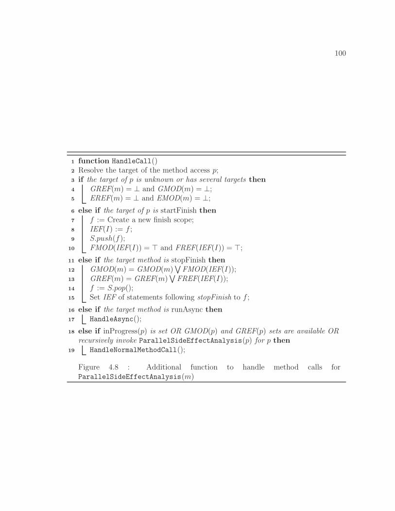
100
function HandleCall()1
Resolve the target of the method access p;2
if the target of p is unknown or has several targets then3
GREF(m) = ⊥ and GMOD(m) = ⊥;4
EREF(m) = ⊥ and EMOD(m) = ⊥;5
else if the target of p is startFinish then6
f := Create a new finish scope;7
IEF(I) := f ;8
S.push(f);9
FMOD(IEF(I)) = ⊤ and FREF(IEF(I)) = ⊤;10
else if the target method is stopFinish then11
GMOD(m) = GMOD(m)∨
FMOD(IEF(I));12
GREF(m) = GREF(m)∨
FREF(IEF(I));13
f := S.pop();14
Set IEF of statements following stopFinish to f ;15
else if the target method is runAsync then16
HandleAsync();17
else if inProgress(p) is set OR GMOD(p) and GREF(p) sets are available OR18
recursively invoke ParallelSideEffectAnalysis(p) for p thenHandleNormalMethodCall();19
Figure 4.8 : Additional function to handle method calls forParallelSideEffectAnalysis(m)
101
For the runAsync function call (as shown in Figure 4.9), we determine the target
runHJTask method and recursively compute side-effects for this method. The GMOD,
GREF, EMOD and EREF sets of the runHJTask method are then unified in the
caller’s enclosing finish scope’s FMOD and FREF sets as shown in steps 8-9 in
Figure 4.9. If the runAsync method call was not enclosed in a finish scope, the
GMOD, GREF, EMOD and EREF sets of runHJTask are unified with the EMOD
and EREF for the caller. This is shown in steps 5-6 in Figure 4.9. Unification with
EMOD and EREF sets indicates that all the side effect for the callee async remain
escaping for the caller. If the async call is enclosed in a finish scope, the async call’s
side effects can only be visible at the end of the finish scope and hence added to
FMOD(IEF(I)) and FREF(IEF(I)) as shown in steps 8-9 in Figure 4.9.
Normal method calls that are not related to parallel constructs (as shown in
Figure 4.9) are handled by unifying the GMOD, GREF, EMOD and EREF sets of
the callee with their corresponding side-effect sets in the caller if there is no IEF for
the call instruction. In case of IEF(I) is undefined, the EMOD and EREF sets of the
callee are unified with respective GMOD and GREF sets of the immediately enclosing
finish scope summary. If the callee is an isolated method or is invoked in an isolated
block, the GMOD and GREF sets are unified with the global AMOD and AREF sets
respectively.
For the example program shown in Figure 4.5 and its corresponding call graph in
Figure 4.6, the final side-effect sets are shown in Table 4.1.
The complexity of Algorithm 4.7 is similar in nature to that of Algorithm 4.3.
Hence, the overall complexity of Algorithm 4.7 is O(N + E) ∗ F , where N accounts
for both normal method calls and parallel constructs in a program.
4.3.1 Discussion
As discussed in Section 4.2.3, we compute global side-effects for isolated blocks and
methods. However, it is possible to refine it with the May-Happens-in-Parallel infor-
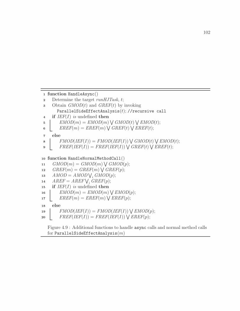
102
function HandleAsync()1
Determine the target runHJTask, t;2
Obtain GMOD(t) and GREF(t) by invoking3
ParallelSideEffectAnalysis(t); //recursive call
if IEF(I) is undefined then4
EMOD(m) = EMOD(m)∨
GMOD(t)∨
EMOD(t);5
EREF(m) = EREF(m)∨
GREF(t)∨
EREF(t);6
else7
FMOD(IEF(I)) = FMOD(IEF(I))∨
GMOD(t)∨
EMOD(t);8
FREF(IEF(I)) = FREF(IEF(I))∨
GREF(t)∨
EREF(t);9
function HandleNormalMethodCall()10
GMOD(m) = GMOD(m)∨
GMOD(p);11
GREF(m) = GREF(m)∨
GREF(p);12
AMOD = AMOD∨
i GMOD(p);13
AREF = AREF∨
i GREF(p);14
if IEF(I) is undefined then15
EMOD(m) = EMOD(m)∨
EMOD(p);16
EREF(m) = EREF(m)∨
EREF(p);17
else18
FMOD(IEF(I)) = FMOD(IEF(I))∨
EMOD(p);19
FREF(IEF(I)) = FREF(IEF(I))∨
EREF(p);20
Figure 4.9 : Additional functions to handle async calls and normal method callsfor ParallelSideEffectAnalysis(m)
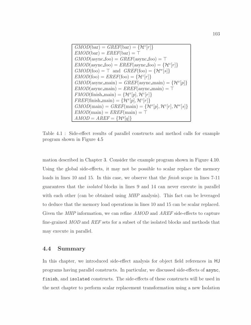
103
GMOD(bar) = GREF(bar) = {Hz[r]}EMOD(bar) = EREF(bar) = ⊤GMOD(async foo) = GREF(async foo) = ⊤EMOD(async foo) = EREF(async foo) = {Hz[r]}GMOD(foo) = ⊤ and GREF(foo) = {Hw[s]}EMOD(foo) = EREF(foo) = {Hz[r]}GMOD(async main) = GREF(async main) = {Hx[p]}EMOD(async main) = EREF(async main) = ⊤FMOD(finish main) = {Hx[p],Hz[r]}FREF(finish main) = {Hx[p],Hz[r]}GMOD(main) = GREF(main) = {Hx[p],Hz[r],Hw[s]}EMOD(main) = EREF(main) = ⊤AMOD = AREF = {Hy[q]}
Table 4.1 : Side-effect results of parallel constructs and method calls for exampleprogram shown in Figure 4.5
mation described in Chapter 3. Consider the example program shown in Figure 4.10.
Using the global side-effects, it may not be possible to scalar replace the memory
loads in lines 10 and 15. In this case, we observe that the finish scope in lines 7-11
guarantees that the isolated blocks in lines 9 and 14 can never execute in parallel
with each other (can be obtained using MHP analysis). This fact can be leveraged
to deduce that the memory load operations in lines 10 and 15 can be scalar replaced.
Given the MHP information, we can refine AMOD and AREF side-effects to capture
fine-grained MOD and REF sets for a subset of the isolated blocks and methods that
may execute in parallel.
4.4 Summary
In this chapter, we introduced side-effect analysis for object field references in HJ
programs having parallel constructs. In particular, we discussed side-effects of async,
finish, and isolated constructs. The side-effects of these constructs will be used in
the next chapter to perform scalar replacement transformation using a new Isolation
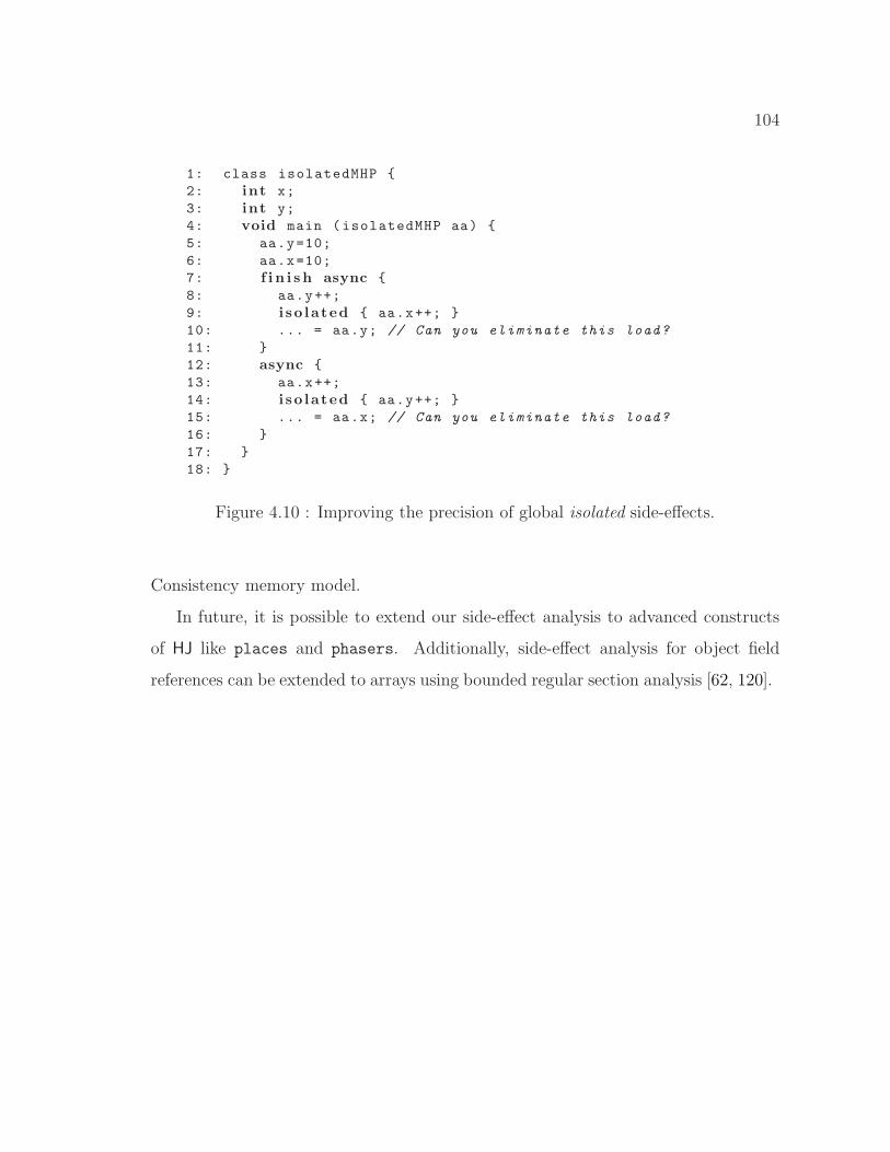
104
1: class isolatedMHP {
2: int x;
3: int y;
4: void main (isolatedMHP aa) {
5: aa.y=10;
6: aa.x=10;
7: f i n i s h async {
8: aa.y++;
9: i so lated { aa.x++; }
10: ... = aa.y; // Can you eliminate this load?
11: }
12: async {
13: aa.x++;
14: i so lated { aa.y++; }
15: ... = aa.x; // Can you eliminate this load?
16: }
17: }
18: }
Figure 4.10 : Improving the precision of global isolated side-effects.
Consistency memory model.
In future, it is possible to extend our side-effect analysis to advanced constructs
of HJ like places and phasers. Additionally, side-effect analysis for object field
references can be extended to arrays using bounded regular section analysis [62, 120].

105
Chapter 5
Isolation Consistency Memory Model and its
Impact on Scalar Replacement
Due to recent software trends in parallel programming languages for multi-core pro-
cessors, it is necessary for a compiler to be aware of the parallel constructs in the
input parallel program to be able to perform any code reordering transformation.
For example, the most commonly used common subexpression elimination (CSE)
data flow framework can not be easily adapted to parallel programs for the following
reasons:
1. Parallel constructs introduce additional kill expressions, i.e., side-effects (ad-
dressed in Chapter 4).
2. Interferences between shared data accesses of multiple threads may prohibit
some subexpression elimination scenarios.
The legality of compiler transformations in the presence of interferences between
shared accesses is typically defined using a memory model. In this chapter, we
introduce a new weaker memory model called Isolation Consistency that permits
several code reordering scenarios compared to many existing weaker memory models.
Using this memory model we present an algorithm to perform scalar replacement for
load elimination of HJ parallel programs.
5.1 Program Transformation and Memory Model
As stated by [78], a parallel program transformation is correct “if the set of possible
observable behaviors of a transformed program is a subset of the possible observable
106
behaviors of the original program.” The possible observable behaviors of a parallel
program and consequently the permissible program transformations are determined
by the underlying memory model. There exists a wide range of memory models.
A strong memory consistency model limits the observable orderings of memory op-
erations among threads and is viewed by programmers as being easier to reason
about, but difficult to implement efficiently. On the other hand, a relaxed or weaker
memory model permits several reordering of memory operations and may be less easy
for programmers to reason about, but is easy to implement efficiently.
Sequential Consistency (SC) defined by [72] introduced the stronger memory
consistency model used in practice. Lamport’s paper states that “the result of any
execution is the same as if the operations of all the processors were executed in some
sequential order, and the operations of each individual processor appear in this se-
quence in the order specified by its program”. This definition of sequential consistency
disallows reordering of memory operations of a thread even if there is no intra-thread
control and data dependence between the memory operations. Consider the example
program shown in Figure 5.1. A standard compiler reordering transformation that
reorders statements 1 and 2 in Thread 1 can produce the result r1 = 2 and r2 = 1
and this result is not consistent in SC model. Note that the statements within
each of the threads Thread 1 and Thread 2 do not have any dependence between
them. This small example demonstrates that sequential consistency limits concurrent
program transformation by disallowing reorderings that are legal under sequential
execution. Additionally, sequential consistency implementations have led to a strong
memory coherence assumption in the hardware, i.e., “all writes to the same location
are serialized in some order and are performed in that order with respect to any
processor” [58]. This enforces some form of serializability on the write operations to
the same locations. These hardware memory coherence assumptions are often ignored
in the software memory consistency model.
The main approach taken in recent memory consistency models is to permit com-
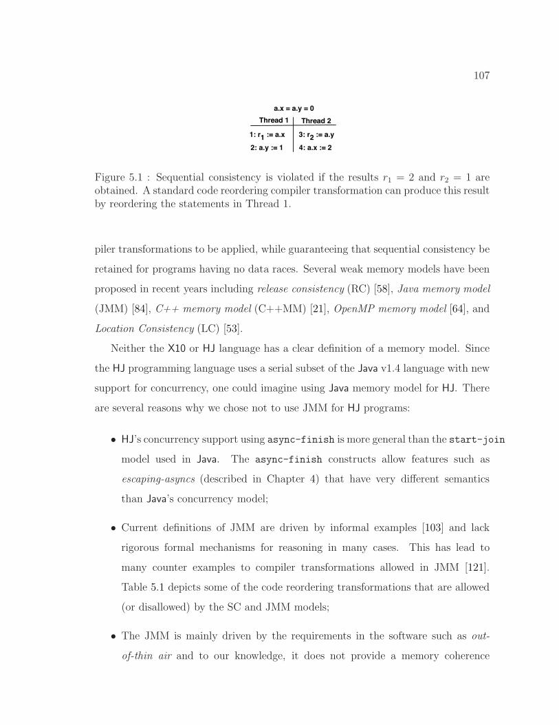
107
a.x = a.y = 0
Thread 1 Thread 2
1: r1 := a.x
2: a.y := 1
3: r2 := a.y
4: a.x := 2
Figure 5.1 : Sequential consistency is violated if the results r1 = 2 and r2 = 1 areobtained. A standard code reordering compiler transformation can produce this resultby reordering the statements in Thread 1.
piler transformations to be applied, while guaranteeing that sequential consistency be
retained for programs having no data races. Several weak memory models have been
proposed in recent years including release consistency (RC) [58], Java memory model
(JMM) [84], C++ memory model (C++MM) [21], OpenMP memory model [64], and
Location Consistency (LC) [53].
Neither the X10 or HJ language has a clear definition of a memory model. Since
the HJ programming language uses a serial subset of the Java v1.4 language with new
support for concurrency, one could imagine using Java memory model for HJ. There
are several reasons why we chose not to use JMM for HJ programs:
• HJ’s concurrency support using async-finish is more general than the start-join
model used in Java. The async-finish constructs allow features such as
escaping-asyncs (described in Chapter 4) that have very different semantics
than Java’s concurrency model;
• Current definitions of JMM are driven by informal examples [103] and lack
rigorous formal mechanisms for reasoning in many cases. This has lead to
many counter examples to compiler transformations allowed in JMM [121].
Table 5.1 depicts some of the code reordering transformations that are allowed
(or disallowed) by the SC and JMM models;
• The JMM is mainly driven by the requirements in the software such as out-
of-thin air and to our knowledge, it does not provide a memory coherence
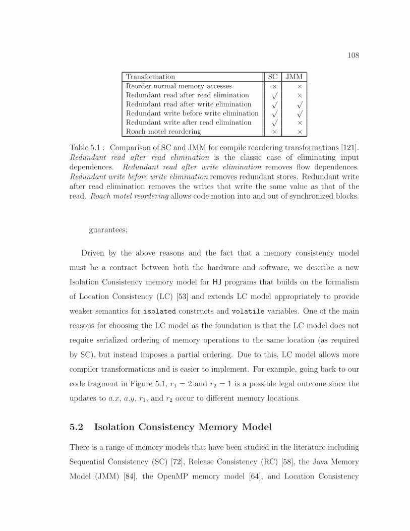
108
Transformation SC JMM
Reorder normal memory accesses × ×Redundant read after read elimination
√ ×Redundant read after write elimination
√ √
Redundant write before write elimination√ √
Redundant write after read elimination√ ×
Roach motel reordering × ×
Table 5.1 : Comparison of SC and JMM for compile reordering transformations [121].Redundant read after read elimination is the classic case of eliminating inputdependences. Redundant read after write elimination removes flow dependences.Redundant write before write elimination removes redundant stores. Redundant writeafter read elimination removes the writes that write the same value as that of theread. Roach motel reordering allows code motion into and out of synchronized blocks.
guarantees;
Driven by the above reasons and the fact that a memory consistency model
must be a contract between both the hardware and software, we describe a new
Isolation Consistency memory model for HJ programs that builds on the formalism
of Location Consistency (LC) [53] and extends LC model appropriately to provide
weaker semantics for isolated constructs and volatile variables. One of the main
reasons for choosing the LC model as the foundation is that the LC model does not
require serialized ordering of memory operations to the same location (as required
by SC), but instead imposes a partial ordering. Due to this, LC model allows more
compiler transformations and is easier to implement. For example, going back to our
code fragment in Figure 5.1, r1 = 2 and r2 = 1 is a possible legal outcome since the
updates to a.x, a.y, r1, and r2 occur to different memory locations.
5.2 Isolation Consistency Memory Model
There is a range of memory models that have been studied in the literature including
Sequential Consistency (SC) [72], Release Consistency (RC) [58], the Java Memory
Model (JMM) [84], the OpenMP memory model [64], and Location Consistency
109
(LC) [53]. It is well known that all these models yield the same semantics for
data-race-free programs, but may exhibit different semantics for parallel programs
with races. A major research challenge lies in dealing with the common case when a
compiler (especially a dynamic compiler) does not know for sure that the input parallel
program is data-race-free. To address this case, we define a weak memory model,
Isolation Consistency (IC), for which the scalar replacement for load elimination
transformation described in Chapter 5 are guaranteed to be correct even in the
presence of data races. They will also be correct for any data-race-free parallel
program with a stronger memory model, but the optimizations may not be correct
for parallel programs with data races that must obey a stronger memory model.
5.2.1 Abstraction
The definition of IC builds on the operational semantics used to define the Location
Consistency (LC) in [53]. Each shared memory location L is modeled as a partial
order using a partially ordered multiset (pomset), state(L) = (S,≺), where S is a
multiset and ≺ ⊆ S × S is a partial order on S. Pomset captures the sequencing of
memory and synchronization operations. Each element e of the multiset S is one of
the following (We use the term worker to refer to the thread/processor executing the
async):
• Write operation: if worker Pi writes value v in location L, it performs a write(Pi, v, L)
operation;
• Finish synchronization: finish constructs in HJ impose a happens-before order-
ing since any async created inside the body of a finish scope completes execution
before the statement after the finish scope is executed. This can be captured
using a directed signal-wait synchronization primitive. If worker P2 needs to
wait for worker P1, then P1 performs a signal(P2) operation and P2 performs a
110
corresponding wait(P1) operation1.
• Isolation: if workers P1, . . . , Pk need exclusive access within an HJ place using
isolated constructs, then each worker performs an acquire(Pi, ∗) operation fol-
lowed by a release(Pi, ∗) operation, where ∗ represents all the shared memory
locations in all the places defined in the isolated scope.
• Volatile Variables: Volatile variables in HJ are similar to Java, i.e., when one
worker writes to a volatile variable, and another worker sees that write, the first
worker is communicating the second about all of the contents of memory up until
it performed the write to that volatile variable. The volatile variables in the
IC model are modeled by wrapping each volatile access using an isolated block.
Hence, an acquire(Pi, ∗) operation followed by a release(Pi, ∗) is performed for
every volatile access.
Let workers(e) be the set of workers involved in the operation e. For example,
for e = write(Pi, v, L), workers(e) = {Pi}. For an e = acquire(Pi, ∗) operation,
most recent release(e) = {e1, . . . , ek}, where ei is the most recent release opera-
tion ei = release(Pi, ∗) performed prior to acquire e. For an wait operation e,
signal sources(e) = {e1, . . . , ek} where ei signals its completion of execution to e
during run-time.
5.2.2 State-Update rules for L
When new memory or synchronization operations are performed, the pomset (S,≺)
is updated. The rules for updating a pomset based on an operation e are provided
using three rules namely default rule, wait rule, and acquire rule. Each of the rules
are described below:
1The signal and wait operations used in the phaser construct of HJ language are different fromthe ones we consider here.
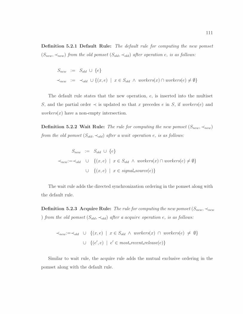
111
Definition 5.2.1 Default Rule: The default rule for computing the new pomset
(Snew,≺new) from the old pomset (Sold,≺old) after operation e, is as follows:
Snew := Sold ∪ {e}
≺new := ≺old ∪ {(x, e) | x ∈ Sold ∧ workers(x) ∩ workers(e) 6= ∅}
The default rule states that the new operation, e, is inserted into the multiset
S, and the partial order ≺ is updated so that x precedes e in S, if workers(e) and
workers(x) have a non-empty intersection.
Definition 5.2.2 Wait Rule: The rule for computing the new pomset (Snew,≺new)
from the old pomset (Sold,≺old) after a wait operation e, is as follows:
Snew := Sold ∪ {e}
≺new:=≺old ∪ {(x, e) | x ∈ Sold ∧ workers(x) ∩ workers(e) 6= ∅}
∪ {(x, e) | x ∈ signal source(e)}
The wait rule adds the directed synchronization ordering in the pomset along with
the default rule.
Definition 5.2.3 Acquire Rule: The rule for computing the new pomset (Snew,≺new
) from the old pomset (Sold,≺old) after a acquire operation e, is as follows:
≺new:=≺old ∪ {(x, e) | x ∈ Sold ∧ workers(x) ∩ workers(e) 6= ∅}
∪ {(e′, e) | e′ ∈ most recent release(e)}
Similar to wait rule, the acquire rule adds the mutual exclusive ordering in the
pomset along with the default rule.
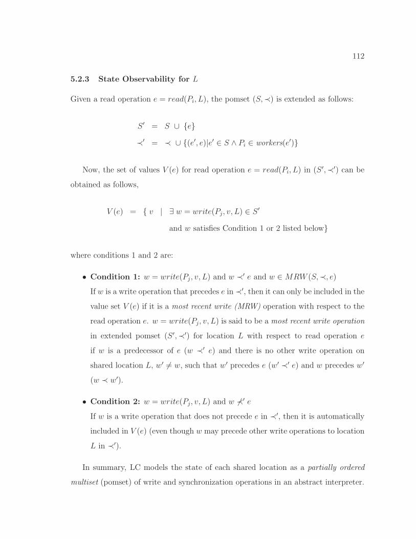
112
5.2.3 State Observability for L
Given a read operation e = read(Pi, L), the pomset (S,≺) is extended as follows:
S ′ = S ∪ {e}
≺′ = ≺ ∪ {(e′, e)|e′ ∈ S ∧ Pi ∈ workers(e′)}
Now, the set of values V (e) for read operation e = read(Pi, L) in (S ′,≺′) can be
obtained as follows,
V (e) = { v | ∃ w = write(Pj, v, L) ∈ S ′
and w satisfies Condition 1 or 2 listed below}
where conditions 1 and 2 are:
• Condition 1: w = write(Pj, v, L) and w ≺′ e and w ∈ MRW (S,≺, e)
If w is a write operation that precedes e in ≺′, then it can only be included in the
value set V (e) if it is a most recent write (MRW) operation with respect to the
read operation e. w = write(Pj, v, L) is said to be a most recent write operation
in extended pomset (S ′,≺′) for location L with respect to read operation e
if w is a predecessor of e (w ≺′ e) and there is no other write operation on
shared location L, w′ 6= w, such that w′ precedes e (w′ ≺′ e) and w precedes w′
(w ≺ w′).
• Condition 2: w = write(Pj, v, L) and w 6≺′ e
If w is a write operation that does not precede e in ≺′, then it is automatically
included in V (e) (even though w may precede other write operations to location
L in ≺′).
In summary, LC models the state of each shared location as a partially ordered
multiset (pomset) of write and synchronization operations in an abstract interpreter.
113
In any execution that satisfies the LC model, the result returned by a read operation
R must belong to the value set of the location, i.e., it must have been written by a
write operation that is a “most recent write” with respect to R in the pomset or a
write operation that is unrelated to R in the pomset.
However, the LC model also placed the restriction that the abstract interpreter
executes each instruction in a thread in its original order, thereby ensuring that
causality is not violated.
In Isolation Consistency (IC), we assume that only the control and data depen-
dences within a thread need to be preserved in the abstract interpreter. Thus the
abstract interpreter is allowed to execute instructions out-of-order within a thread so
long as intra-thread dependences are not violated. These intra-thread dependences
are defined using a weak atomicity model [85] which ensures the correct ordering of
load and store operations from multiple threads when they occur in isolated sections.
For load and store operations that occur outside an isolated section, the only inter-
thread ordering constraints arise from the “happens-before” relationships enforced by
the finish construct.
5.2.4 Example Scenarios
Consider the four example parallel code fragments shown in Figure 5.2. Cases 1 and
2 demonstrate the potential for scalar replacement for load elimination across async
constructs, Case 3 across a finish construct, and Case 4 across isolated constructs.
In each case, we want to know if the load of a.f in statement 4 can be eliminated
by substituting the value of a prior store operation. (The . . . notation represents
computations that do not contain accesses to any instances of field f.) The IC model
permits scalar replacement in all four cases, but that is not the case for the SC and
JMM models. Cases 1 and 4 have no data races, but for the non-IC memory models,
the onus is on the compiler to establish that there are no data races in those cases.
Case 1 appears to be an easy case because the async body is assumed to not
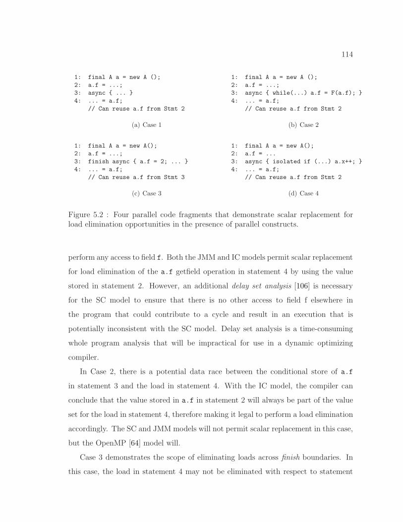
114
1: final A a = new A ();
2: a.f = ...;
3: async { ... }
4: ... = a.f;
// Can reuse a.f from Stmt 2
(a) Case 1
1: final A a = new A ();
2: a.f = ...;
3: async { while(...) a.f = F(a.f); }
4: ... = a.f;
// Can reuse a.f from Stmt 2
(b) Case 2
1: final A a = new A();
2: a.f = ...;
3: finish async { a.f = 2; ... }
4: ... = a.f;
// Can reuse a.f from Stmt 3
(c) Case 3
1: final A a = new A();
2: a.f = ...
3: async { isolated if (...) a.x++; }
4: ... = a.f;
// Can reuse a.f from Stmt 2
(d) Case 4
Figure 5.2 : Four parallel code fragments that demonstrate scalar replacement forload elimination opportunities in the presence of parallel constructs.
perform any access to field f. Both the JMM and IC models permit scalar replacement
for load elimination of the a.f getfield operation in statement 4 by using the value
stored in statement 2. However, an additional delay set analysis [106] is necessary
for the SC model to ensure that there is no other access to field f elsewhere in
the program that could contribute to a cycle and result in an execution that is
potentially inconsistent with the SC model. Delay set analysis is a time-consuming
whole program analysis that will be impractical for use in a dynamic optimizing
compiler.
In Case 2, there is a potential data race between the conditional store of a.f
in statement 3 and the load in statement 4. With the IC model, the compiler can
conclude that the value stored in a.f in statement 2 will always be part of the value
set for the load in statement 4, therefore making it legal to perform a load elimination
accordingly. The SC and JMM models will not permit scalar replacement in this case,
but the OpenMP [64] model will.
Case 3 demonstrates the scope of eliminating loads across finish boundaries. In
this case, the load in statement 4 may not be eliminated with respect to statement
115
2. The finish scope in statement 3 demarcates the completion of the execution of
the async body in statement 3 and hence is visible to the rest of the program.
Case 4 shows the effect of scalar replacement for load elimination in the presence
of isolated constructs. The load in statement 4 cannot be eliminated in the SC and
JMM models due to the isolated construct. However, if we can analyze the side
effect of the isolated construct, we should able to eliminate the load in statement 4.
In this case,the async only updates field a.x. Hence, eliminating the load of a.f in
statement 4 is safe in the IC model.
5.3 Scalar Replacement for Load Elimination
Now, we will describe the scalar replacement for load elimination algorithm that
analyzes parallel constructs. It follows the same basic steps of the load elimination
algorithm described in Section 2.6, but embeds side-effects of parallel constructs and
permits scalar replacement using isolation consistency model described in the previous
section. The side-effects for method calls and parallel constructs are computed using
the algorithms presented in Chapter 4.
Algorithm 5.3 presents the complete scalar replacement for load elimination algo-
rithm in the presence of parallel constructs. Steps 4-21 determine the type of method
call based on the parallel constructs and inserts appropriate pseudo-def and pseudo-
use instructions for their GMOD and GREF sets. Each entry into the isolated block
is annotated with pseudo-defs to fields in AMOD. This prohibits any load reuse
in the isolated block for fields that may be modified in any isolated scope. Each
exit of an isolated construct is annotated with pseudo-uses of fields in AREF. This
permits loads to be eliminated in and after the isolated block exit. startFinish and
runAsync method calls are handled by side-effect analysis and act as a no-op for load
elimination algorithm. At stopFinish, pseudo-def and pseudo-use instructions are
added for FMOD and FREF finish side-effect sets of the current finish scope. Other
normal method calls insert pseudo-def and uses for GMOD and GREF summary sets
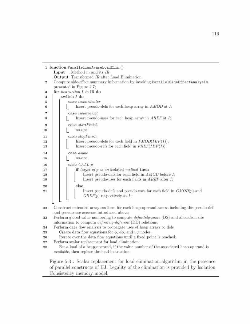
116
function ParallelismAwareLoadElim ()1
Input : Method m and its IR
Output: Transformed IR after Load EliminationCompute side-effect summary information by invoking ParallelSideEffectAnalysis2
presented in Figure 4.7;for instruction I in IR do3
switch I do4
case isolatedenter5
Insert pseudo-defs for each heap array in AMOD at I;6
case isolatedexit7
Insert pseudo-uses for each heap array in AREF at I;8
case startFinish9
no-op;10
case stopFinish11
Insert pseudo-defs for each field in FMOD(IEF (I));12
Insert pseudo-refs for each field in FREF(IEF (I));13
case async14
no-op;15
case CALL p16
if target of p is an isolated method then17
Insert pseudo-defs for each field in AMOD before I;18
Insert pseudo-uses for each fields in AREF after I;19
else20
Insert pseudo-defs and pseudo-uses for each field in GMOD(p) and21
GREF(p) respectively at I;
Construct extended array ssa form for each heap operand access including the pseudo-def22
and pseudo-use accesses introduced above;Perform global value numbering to compute definitely-same (DS) and allocation site23
information to compute definitely-different (DD) relations;Perform data flow analysis to propagate uses of heap arrays to defs;24
Create data flow equations for φ, dφ, and uφ nodes;25
Iterate over the data flow equations until a fixed point is reached;26
Perform scalar replacement for load elimination;27
For a load of a heap operand, if the value number of the associated heap operand is28
available, then replace the load instruction;
Figure 5.3 : Scalar replacement for load elimination algorithm in the presenceof parallel constructs of HJ. Legality of the elimination is provided by IsolationConsistency memory model.
117
if the target of the method call is not an isolated method. Otherwise, pseudo-defs for
fields in IMOD and pseudo-uses for fields in IREF are inserted before and after the
method call.
Steps 22-28 in Algorithm 5.3 first construct an extended array ssa form repre-
sentation of the IR over which a global value numbering is performed to compute
object accesses that may be definitely-same (DS) or definitely-different (DD). In
Step 24, a data flow analysis is performed that propagates uses of heap operands to
their definition points. Finally, actual load elimination is performed by replacing the
memory load operation by a compiler generated temporary in cases where the load
is already fully available. The steps 22-28 are described in details in [52].
5.3.1 Example
Consider the example program shown in Figure 5.4. The same example was used
in Chapter 4 to demonstrate side-effect analysis of parallel constructs. Table 4.1 in
Section 4.3 summarizes the side-effects of both method calls and parallel constructs.
Using these side-effect information and the scalar replacement algorithm with IC
memory model described in Algorithm 5.3 produces the transformed code shown in
Figure 5.5. Note that, p x is used as a scalar variable for replacing a memory load
of p.x. The memory load operations on lines 8, 9, 12, 16, and 25 can now be scalar
replaced. The memory load on line 15 can not be scalar replaced due to the finish
ordering imposed by the finish construct on lines 4-14. One interesting scenario is
that the memory load on line 12 can be scalar replaced even though the program can
have a data race with respect to the async created on line 6.
5.4 Summary
This chapter introduces a new weak memory consistency model as Isolation Consis-
tency memory model (IC) that favors compiler reordering transformations for racy
programs while producing sequentially consistent behaviors for race-free programs.
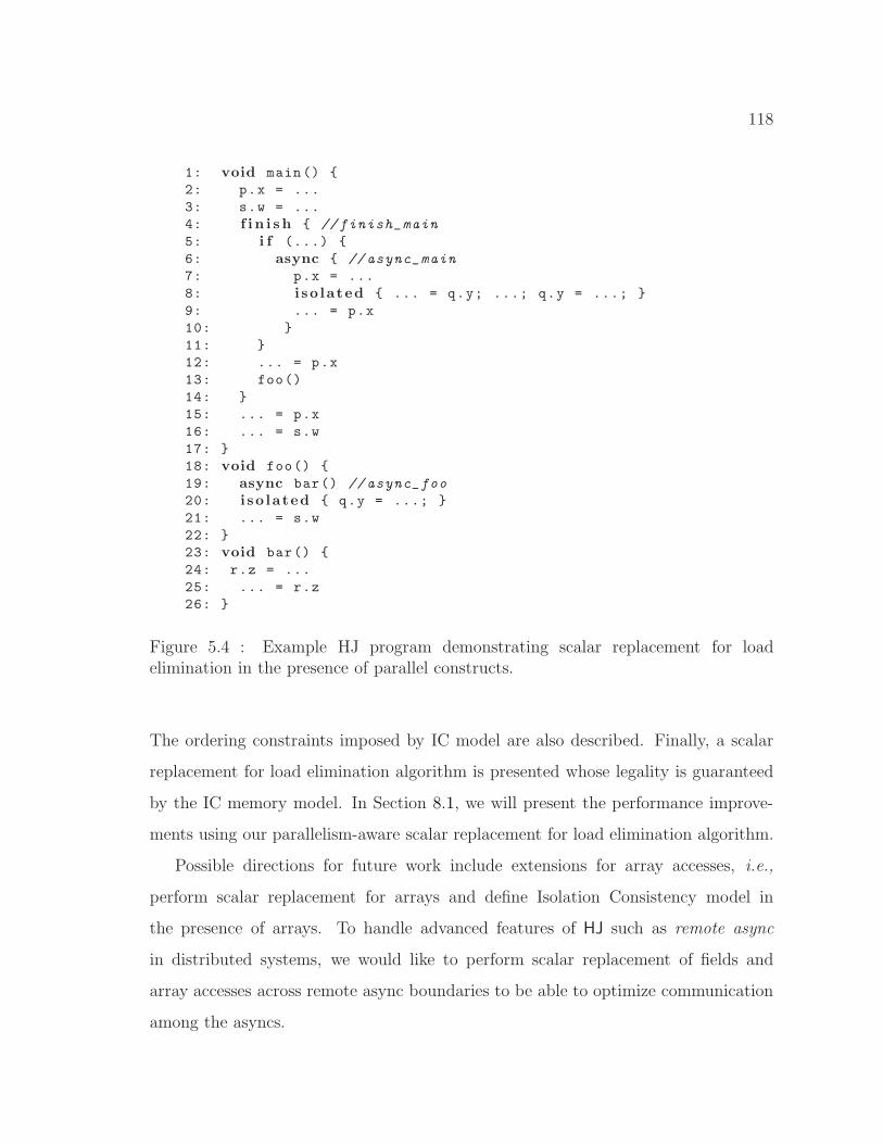
118
1: void main() {
2: p.x = ...
3: s.w = ...
4: f i n i s h { // finish_main
5: i f (...) {
6: async { // async_main
7: p.x = ...
8: i so lated { ... = q.y; ...; q.y = ...; }
9: ... = p.x
10: }
11: }
12: ... = p.x
13: foo()
14: }
15: ... = p.x
16: ... = s.w
17: }
18: void foo() {
19: async bar() // async_foo
20: i so lated { q.y = ...; }
21: ... = s.w
22: }
23: void bar() {
24: r.z = ...
25: ... = r.z
26: }
Figure 5.4 : Example HJ program demonstrating scalar replacement for loadelimination in the presence of parallel constructs.
The ordering constraints imposed by IC model are also described. Finally, a scalar
replacement for load elimination algorithm is presented whose legality is guaranteed
by the IC memory model. In Section 8.1, we will present the performance improve-
ments using our parallelism-aware scalar replacement for load elimination algorithm.
Possible directions for future work include extensions for array accesses, i.e.,
perform scalar replacement for arrays and define Isolation Consistency model in
the presence of arrays. To handle advanced features of HJ such as remote async
in distributed systems, we would like to perform scalar replacement of fields and
array accesses across remote async boundaries to be able to optimize communication
among the asyncs.
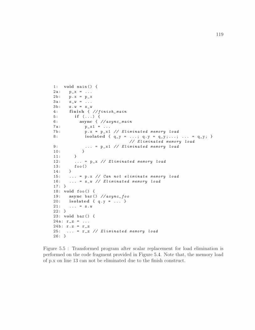
119
1: void main() {
2a: p_x = ...
2b: p.x = p_x
3a: s_w = ...
3b: s.w = s_w
4: f i n i s h { // finish_main
5: i f (...) {
6: async { // async_main
7a: p_x1 = ...
7b: p.x = p_x1 // Eliminated memory load
8: i so lated { q_y = ...; q.y = q_y;...; ... = q_y; }
// Eliminated memory load
9: ... = p_x1 // Eliminated memory load
10: }
11: }
12: ... = p_x // Eliminated memory load
13: foo()
14: }
15: ... = p.x // Can not eliminate memory load
16: ... = s_w // Eliminated memory load
17: }
18: void foo() {
19: async bar() // async_foo
20: i so lated { q.y = ... }
21: ... = s.w
22: }
23: void bar() {
24a: r_z = ...
24b: r.z = r_z
25: ... = r_z // Eliminated memory load
26: }
Figure 5.5 : Transformed program after scalar replacement for load elimination isperformed on the code fragment provided in Figure 5.4. Note that, the memory loadof p.x on line 13 can not be eliminated due to the finish construct.
120
Chapter 6
Space-Efficient Register Allocation
Typically, a register allocator consists of two tasks: allocation and assignment. Allo-
cation ensures that no more than k symbolic registers are residing in physical registers
at any program point (where k is the total number of physical registers available in
the target machine), assignment produces the actual physical register names required
to generate the executable code. Both these tasks are NP-hard at the global (i.e.,
procedure) level.
Today’s architectures pose new challenges to register allocation due to hardware
features such as register classes, register aliases, pre-coloring, and register pairs. For
example, the Intel x86 architecture provides eight integer physical registers, of which
six are usable by the compiler. These six physical registers are further divided into
four register classes based on calling conventions and 8-bit operand accesses. To
produce high-quality machine code, a register allocator must consider these hardware
features in both the allocation and assignment phases.
In this chapter, we make the following contributions:
1. We introduce a Bipartite Liveness Graph (BLG) representation as an alternative
to the interference graph (IG) representation. Allocation with the BLG is for-
mulated as an optimization problem and a greedy heuristic is presented to solve
it. Our allocation phase is independent of the move-coalescing optimization
that is usually performed along with allocation in an IG based Graph Coloring
algorithm.
2. We present a spill-free register assignment that reduces the number of spill in-
structions by using register-to-register move and exchange instructions wherever
121
possible to maximize the use of registers.
3. We formulate spill-free register assignment with move coalescing as a combined
optimization problem that maximizes the benefits of move coalescing while
finding an assignment for every symbolic register. Move coalescing is performed
on a Coalesce Graph (CG) that models both IR move instructions and additional
register-to-register moves/exchanges needed to generate correct code. A local
greedy heuristic is presented to address the assignment optimization problem.
4. We extend the register assignment approach from (3) above to handle regis-
ter classes. An optimization version of the assignment problem is presented
that minimizes the additional spilled symbolic registers and at the same time
maximizes the benefits of move coalescing. A prioritized bucket-based greedy
heuristic is presented to address this problem.
5. Finally, we present an Extended Linear Scan (ELS) register allocation algorithm
that avoids building the BLG explicitly to save space. ELS retains the compile
time and space efficiency of Linear Scan register allocation algorithms.
6.1 Notions Revisited
For convenience, a program point can be split into two program points based on the
values read and written at that program point [105]. A register allocation problem
can then be defined with respect to the split program points as follows.
Definition 6.1.1 Each program point p is split into p− and p+, where p− consists of
the variables that are read at p and p+ consists of the variables that are written at p.
Definition 6.1.2 Given a set of symbolic registers, S, and k uniform physical reg-
isters that are independent and interchangeable, determine if it is possible to assign
each symbolic register s ∈ S to a physical register at every program point where s
122
is live. If so, report the assignment as reg(s, x) that indicates the physical register
assigned to s at each program point x.
The number of simultaneously live symbolic registers at a program point p is
denoted by numlive(p). MAXLIV E represents the maximum number of simultane-
ously live symbolic registers in any program point. A program point p is said to be
constrained if numlive(p) > k. In the presence of register classes, we call a program
point p as constrained if it violates any of the register requirements of any of the
register classes of the symbolic registers that are live at p.
Linear Scan (LS) [100, 105, 119] is a compile time and space efficient approach
to register allocation that is suitable for dynamic compilation. It assumes a linear
ordering of the IR instructions (typically depth-first order [4]). The central data
structure in LS is the notion of live interval. A live interval may contain program
points where a variable v may not be live, i.e., it does not contain any useful value
but it is included in the live interval of v. The sub-interval during which a variable
is not live is known as a hole [119].
Definition 6.1.3 [x, y] is a basic interval for variable v (denoted as BI(v)) iff ∀p,p ≥ x, p ≤ y and v is live at p. Note that BI(v) does not include any holes. Lo(BI(v))
and Hi(BI(v)) denote the unique start and end points respectively of basic interval
BI(v).
Definition 6.1.4 A compound interval for a variable v (denoted as CI(v)) consists
of a set of basic intervals for v. Note that CI(v) accommodates holes.
Definition 6.1.5 Two basic intervals, [x1, y1] and [x2, y2], are said to be intersecting
if one of the following holds:
1. x2 ≥ x1 and x2 ≤ y1
2. y2 ≥ x1 and y2 ≤ y1
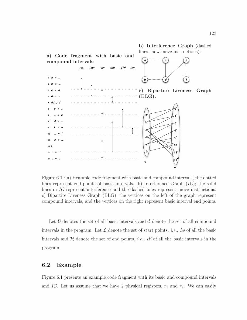
123
a) Code fragment with basic andcompound intervals:
1 a = ...
2 b = ...
3 c = a
4 d = b
5 if (...) {
6 e = ...
7 ... = c
8 d = ...
9 f = e
10 ... = f
11 c = ...
12 }
13 ... = d
14 ... = c
C(a) (b)C C(c) C C C(d) (e) (f)
b) Interference Graph (dashedlines show move instructions):
a
b d f
ec
c) Bipartite Liveness Graph(BLG):
a
3-
4-
5-
7-
9-
10-
13-
14-
b
c
d
e
f
U
V
Figure 6.1 : a) Example code fragment with basic and compound intervals; the dottedlines represent end-points of basic intervals. b) Interference Graph (IG); the solidlines in IG represent interference and the dashed lines represent move instructions.c) Bipartite Liveness Graph (BLG); the vertices on the left of the graph representcompound intervals, and the vertices on the right represent basic interval end points.
Let B denotes the set of all basic intervals and C denote the set of all compound
intervals in the program. Let L denote the set of start points, i.e., Lo of all the basic
intervals and H denote the set of end points, i.e., Hi of all the basic intervals in the
program.
6.2 Example
Figure 6.1 presents an example code fragment with its basic and compound intervals
and IG. Let us assume that we have 2 physical registers, r1 and r2. We can easily
124
see that the IG has a clique of size 3, i.e., the cycle comprising of nodes c, d, and e.
Now, consider a Graph Coloring register allocator that performs coalescing along with
allocation. Both aggressive [35] and conservative [25, 28] coalescing will be able to
eliminate the move edges (a, c), (b, d), and (e, f) without increasing the colorability of
the original interference graph. Since there are two physical registers, we have to spill
one among the coalesced nodes ac, bd, and ef . Coalescing has worsened the situation
because it would have sufficed to spill just one of the nodes in the coalesced node that
is part of the cycle, e.g., it would have been enough to just spill d instead of bd. The
un-coalescing approach used in an optimistic coalescing technique [96] will be able to
just spill one of the nodes involved in the cycle as it tries all possible combinations
of assigning colors to individual nodes of a potentially spilled coalesced node. The
points to note here are that we can not color the IG using 2 physical registers and
that opportunities for coalescing can be missed due to not being able to color certain
nodes.
A close look at the code and the intervals reveal the fact that none of the program
points have more than 2 variables live simultaneously. If this is the case, two questions
come to mind: 1) can we generate spill-free code with 2 physical registers that does
not give up any coalescing of symbolic registers? 2) if the answer to the first question
is yes, then why did Graph Coloring generate spill code and also miss the coalescing
opportunity?
The answer to the first question is yes. The Bipartite Liveness Graph (BLG)
shown in Figure 6.1(c) captures the fact that every basic interval end point in V
has degree less than or equal to 2 indicating no more than 2 compound intervals
are simultaneously live. Using this information, the following register assignment is
possible:
reg([1+, 3−]) = r1, reg([2+, 4−]) = r2, reg([4+, 5−]) = r2, reg([3+, 7−]) = r1,
reg([6+, 9−]) = r2, reg([9+, 10−]) = r2, reg([8+, 13−]) = r1,
and reg([11+, 14−]) = r2.
125
This assignment requires an additional register exchange operation since the reg-
ister assignment for the basic intervals of both CI(c) and CI(d) were exchanged
when the code after the if condition was executed, i.e., CI(c) : reg([3+, 7−]) =
r1, reg([11+, 14−]) = r2 and CI(d) : reg([4+, 5−]) = r2, reg([8+, 13−]) = r1. We need
to insert an exchg r1, r2 instruction on the control flow edge between 4 and 13. Also
note that none of the coalescing opportunities on lines 3, 4 and 9 were given up during
such an assignment.
Now let us try to answer the second question. Looking at the code fragment,
we observe that in program point 13−, d interferes with two values of c assigned on
lines 3 and 11. Similarly, c interferes with two values of d assigned on lines 4 and 8.
During runtime if the if-branch is taken then assignments on lines 8 and 11 will be
visible to the code following the if condition, otherwise assignments on lines 3 and 4
will be visible. This notion can not be precisely captured using the definition of live
ranges in an interference graph unless we convert the program to SSA form. However,
an SSA based approach inserts extra copy statements during out-of-ssa translation
which pose an additional challenge as discussed in Section 6.3.
Figure 6.2 presents another example code fragment with its basic and compound
intervals and IG. Similar to the previous example, we can easily see that the IG has a
clique of size 3, i.e., the cycle comprising of nodes b, c, and d. Graph Coloring register
allocator will end up spilling one of the nodes b, c or d and give up the corresponding
coalescing opportunity. However, it is possible to generate spill-free assignment for
this program that does not need to spill any variable.
The following assignment is possible:
reg([1+, 2−])=r1, reg([2+, 5−])=r1, reg([4+, 7−]) = r2, reg([6+, 7−])=r1,
reg([8+, 10−])=r1, reg([11+, 13−])=r1, reg([9+, 14−])=r2, reg([13+, 15−])=r1,
and reg([14+, 16−])=r2.
This assignment requires an additional register-to-register move as the two basic inter-
vals of the compound interval CI(d) are allocated in two different physical registers,
126
i.e., reg([6+, 7−])=r1 and reg([9+, 14−])=r2. We need mov r1, r2 instruction to be
added on the control flow edge between program points 7 and 13. Additionally, we
observe that the all the move instructions on lines 2, 13 and 14 can be removed in the
generated code as both the source and destination have the same physical register. If
we analyze the code fragment, we observe that b interferes with c on the true branch
of the if condition and b interferes with d on the false branch. During runtime only
one path is taken and hence, one of the interferences but not both will be held. Once
again, this notion was not precisely captured in the notion of live ranges in an IG
representation.
The above examples illustrate cases in which none of the program points has more
than 2 simultaneously live symbolic registers, yet the interference graph contains a
clique of size 3 (forcing the need to spill a symbolic register). This raises a question
about the general approach of formulating the register allocation problem as the graph
coloring problem on the IG using live ranges. Even though the interference graph
provides a global view of the program, it is less precise than intervals, and is also
known to be a space and time bottleneck. Additionally, when coalescing is performed
along with register allocation on an interference graph, the degree of some nodes may
increase. (The colorability of the interference graph may increase if we do not use
conservative coalescing.) This unnecessarily complicates the allocation phase of the
register allocation process. We believe that the allocation phase should only focus
on choosing a set of symbolic registers that need to be allocated to physical registers
and should have nothing to do with coalescing. Coalescing should ideally be a part
of the assignment phase of a register allocation algorithm.
6.3 Overall Approach
The register allocator presented in this chapter is depicted in Figure 6.3. The first step
in the allocator is to build data structures for Basic Intervals, Compound Intervals
and the Bipartite Liveness Graph (BLG) defined in Section 6.4. Then, allocation is
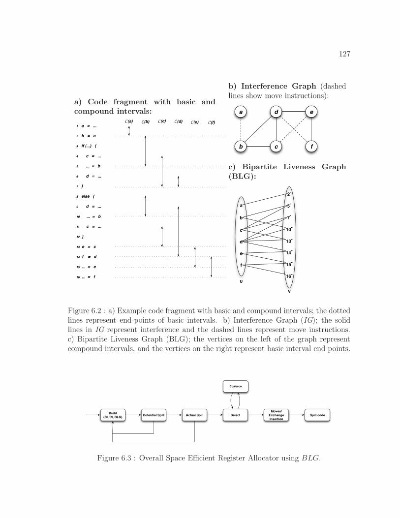
127
a) Code fragment with basic andcompound intervals:
1 a = ...
2 b = a
3 if (...) {
4 c = ...
5 ... = b
6 d = ...
7 }
8 else {
9 d = ...
10 ... = b
11 c = ...
12 }
13 e = c
14 f = d
15 ... = e
16 ... = f
C(a) C(b) (c) (d)C C C(e) (f)C
b) Interference Graph (dashedlines show move instructions):
a
b c
d e
f
c) Bipartite Liveness Graph(BLG):
a
2-
5-
7-
10-
13-
14-
15-
b
c
d
e
f
U
V
16-
Figure 6.2 : a) Example code fragment with basic and compound intervals; the dottedlines represent end-points of basic intervals. b) Interference Graph (IG); the solidlines in IG represent interference and the dashed lines represent move instructions.c) Bipartite Liveness Graph (BLG); the vertices on the left of the graph representcompound intervals, and the vertices on the right represent basic interval end points.
Build
(BI, CI, BLG)Potential Spill Actual Spill Select
Coalesce
Moves/
Exchange
Insertion
Spill code
Figure 6.3 : Overall Space Efficient Register Allocator using BLG.
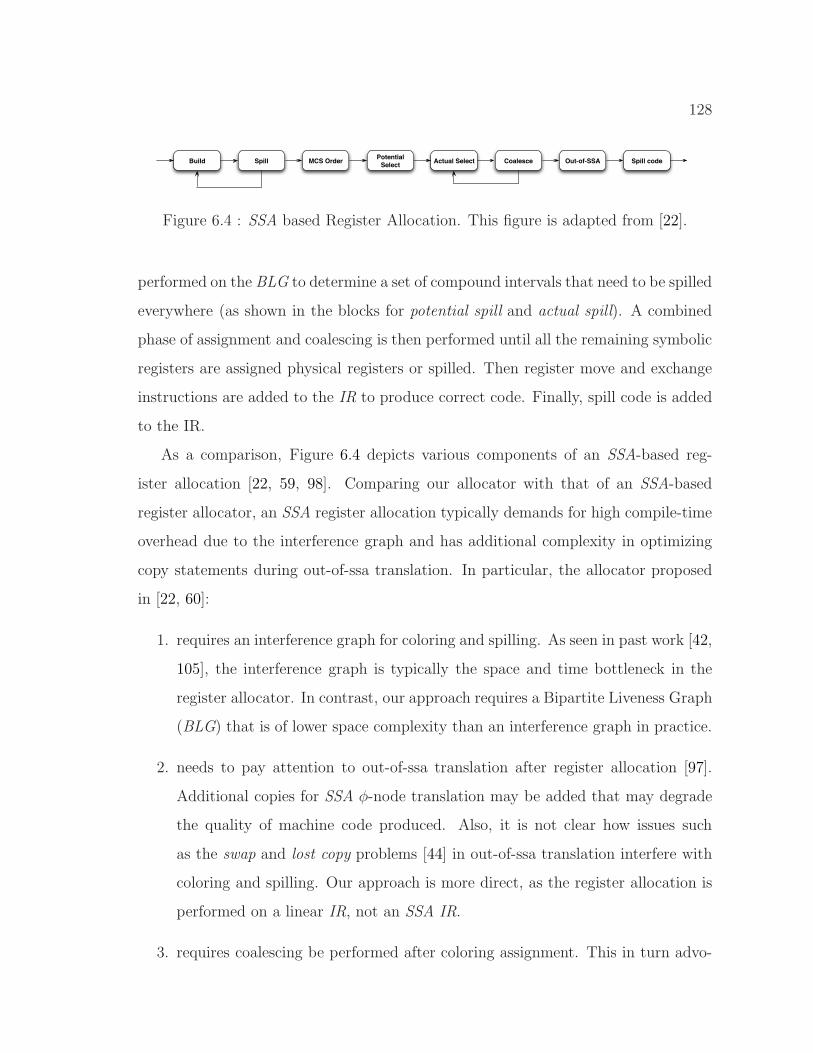
128
Build Spill MCS Order Actual Select Coalesce Out-of-SSA Spill codePotential
Select
Figure 6.4 : SSA based Register Allocation. This figure is adapted from [22].
performed on the BLG to determine a set of compound intervals that need to be spilled
everywhere (as shown in the blocks for potential spill and actual spill). A combined
phase of assignment and coalescing is then performed until all the remaining symbolic
registers are assigned physical registers or spilled. Then register move and exchange
instructions are added to the IR to produce correct code. Finally, spill code is added
to the IR.
As a comparison, Figure 6.4 depicts various components of an SSA-based reg-
ister allocation [22, 59, 98]. Comparing our allocator with that of an SSA-based
register allocator, an SSA register allocation typically demands for high compile-time
overhead due to the interference graph and has additional complexity in optimizing
copy statements during out-of-ssa translation. In particular, the allocator proposed
in [22, 60]:
1. requires an interference graph for coloring and spilling. As seen in past work [42,
105], the interference graph is typically the space and time bottleneck in the
register allocator. In contrast, our approach requires a Bipartite Liveness Graph
(BLG) that is of lower space complexity than an interference graph in practice.
2. needs to pay attention to out-of-ssa translation after register allocation [97].
Additional copies for SSA φ-node translation may be added that may degrade
the quality of machine code produced. Also, it is not clear how issues such
as the swap and lost copy problems [44] in out-of-ssa translation interfere with
coloring and spilling. Our approach is more direct, as the register allocation is
performed on a linear IR, not an SSA IR.
3. requires coalescing be performed after coloring assignment. This in turn advo-
129
cates the need for re-coloring in the IG during the coalescing pass, leading to
color clashes [60]. Backtracking on color assignments in the IG is an expensive
operation that may be undesirable in a dynamic compilation environment. In
contrast, our approach performs move coalescing over a Coalesce Graph that
combines the moves present in the IR and the moves that are needed by the
assignment phase into a single optimization problem. The assignment and
coalescing passes go hand-in-hand in our approach.
4. may require additional heuristics such as those described in [110] on the in-
terference graph to handle advanced features like register classes and register
aliasing. These features are easier to model in a BLG than on an interference
graph.
6.4 Allocation using Bipartite Liveness Graphs
The Bipartite Liveness Graph (BLG) is a new representation that captures program-
point specific liveness information as an alternative to the interference graph. We take
an all-or-nothing approach for spills, i.e., if spilled, every occurrence of the symbolic
register in the program will perform either a fetch or a store of the memory location
assigned to the symbolic register.
Definition 6.4.1 A Bipartite Liveness Graph (BLG) is a undirected weighted bipar-
tite graph, G = 〈U ∪V, E〉, where V denotes all the basic interval end points1 in H, U
denotes all the compound intervals in C and an edge e = (u, v) ∈ E indicates that the
compound interval u ∈ U is live at the interval end point v ∈ V . Each u ∈ U has an
associated non-negative weight SPILL(u) that denotes the spill cost of u. Similarly,
each v ∈ V has an associated non-negative weight FREQ(v) that denotes the execution
frequency of the IR instruction associated with basic interval end point v.
1The choice of interval end points is arbitrary. We could have used interval start points instead.
130
Definition 6.4.2 Allocation Optimization Problem: Given a BLG, G, and k
uniform physical registers, find a spill set S ⊆ U and G′ ⊆ G induced by S such that:
(1) ∀v ∈ V , v is unconstrained, i.e., DEGREE(v) ≤ k; and (2)∑
s∈S SPILL(s)
is minimized. For each compound interval s ∈ S and basic interval b ∈ s, set
spilled(b) := true.
Note that, it is a waste of space to capture liveness information at every program
point in the BLG. From an allocation perspective, it suffices to consider either the
basic interval start points alone, or end points alone but not both. This is because
spilling/allocation decisions only need to be taken at those points.
Given a BLG, the register allocation problem now reduces to an optimization
problem whose solution ensures no more than k physical registers are needed at
every interval end point and at the same time spills as few compound intervals
as possible. Algorithm 6.5 provides a greedy heuristic that solves the allocation
optimization problem. Steps 3-12 choose Potential Spill (as shown in Figure 6.3)
candidates using a max-min heuristic. Steps 13-17 unspill some of the potential spill
candidates producing Actual Spill (as shown in Figure 6.3) candidates. Depending
on the quality of potential spill candidate selection, the unspilling of spill candidates
provide a way of rectifying the obvious spilling decisions (akin to unspilling in Graph
Coloring).
Theorem 6.4.3 Algorithm 6.5 ensures that every program point has k or fewer
symbolic registers simultaneously live.
Proof: The algorithm continues to execute the while loop in Steps 3-12 until there
are constrained nodes v ∈ V in the BLG. This is guaranteed by Steps 3, 10, and 12.
�
Theorem 6.4.4 Algorithm 6.5 requires O(|B| ∗ |C|) space.
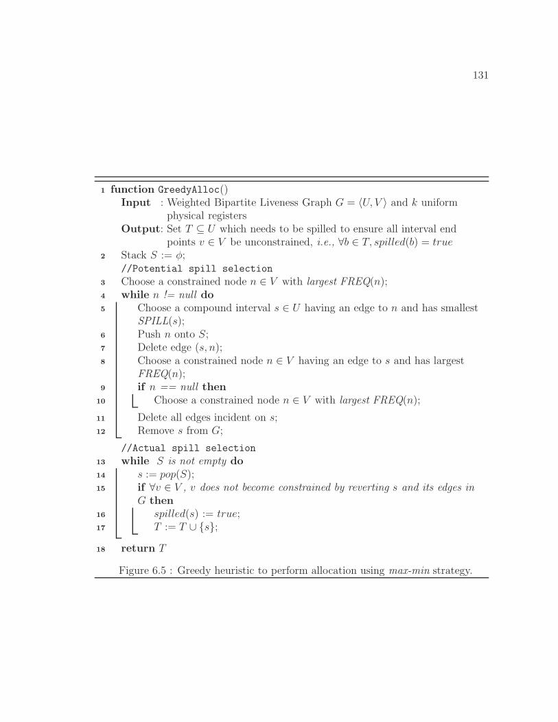
131
function GreedyAlloc()1
Input : Weighted Bipartite Liveness Graph G = 〈U, V 〉 and k uniformphysical registers
Output: Set T ⊆ U which needs to be spilled to ensure all interval endpoints v ∈ V be unconstrained, i.e., ∀b ∈ T, spilled(b) = true
Stack S := φ;2
//Potential spill selection
Choose a constrained node n ∈ V with largest FREQ(n);3
while n != null do4
Choose a compound interval s ∈ U having an edge to n and has smallest5
SPILL(s);Push n onto S;6
Delete edge (s, n);7
Choose a constrained node n ∈ V having an edge to s and has largest8
FREQ(n);if n == null then9
Choose a constrained node n ∈ V with largest FREQ(n);10
Delete all edges incident on s;11
Remove s from G;12
//Actual spill selection
while S is not empty do13
s := pop(S);14
if ∀v ∈ V , v does not become constrained by reverting s and its edges in15
G thenspilled(s) := true;16
T := T ∪ {s};17
return T18
Figure 6.5 : Greedy heuristic to perform allocation using max-min strategy.
132
Proof: The main data structure for Algorithm 6.5 is the BLG. A BLG, G = 〈U ∪V, E〉 can represented using an adjacency list representation that uses O(|U | + |V |+|E|) space. Since |U | = |C|, |V | = |B|, and |E| in the worst case can be |B| ∗ |C|, the
overall space requirement for a BLG is —O(|B| ∗ |C|). Additional |C| stack space is
required for unspilling.�
Note that though O(|B| ∗ |C|) is a worst-case quadratic size, in practice, we do not
need to consider every interval end point of the program in a BLG for Algorithm 6.5
– only constrained end points are sufficient. Hence, we expect the BLG to be a sparse
graph with even lower space requirements.
Theorem 6.4.5 Algorithm 6.5 requires O(|B| ∗ (MAXLIV E − k) ∗ |C|) time.
Proof: Every interval end point of B is traversed at most (MAXLIV E −k) number
of times to make it unconstrained. Each visit of an interval end point needs to visit all
its outgoing edges and choose a minimum spill cost compound interval. This requires
at most |C| edge visits.�
6.4.1 Eager Heuristic
As a comparison to the heuristic presented in Figure 6.5, we present another greedy
heuristic in Figure 6.6 to perform eager allocation. This approach is compile-time
efficient, as each interval end point in BLG is traversed exactly once. The basic
idea is to find the next largest frequency interval end point and make the end point
unconstrained before traversing another interval end point.
Theorem 6.4.6 Algorithm 6.6 requires O(|B| ∗ |C|) time.
Proof: Every interval end point of B is traversed exactly once. Each such visit
needs to visit all its outgoing edges and choose a set of minimum spill cost compound
intervals to make the end point unconstrained. This requires at most |C| edge visits.�
The key advantage of performing register allocation using BLG is that the allo-
cation process only focuses on spilling decisions to produce unconstrained interval
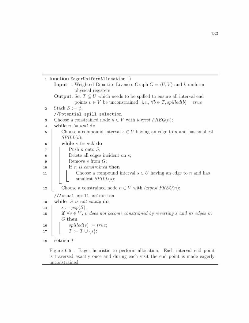
133
function EagerUniformAllocation ()1
Input : Weighted Bipartite Liveness Graph G = 〈U, V 〉 and k uniformphysical registers
Output: Set T ⊆ U which needs to be spilled to ensure all interval endpoints v ∈ V be unconstrained, i.e., ∀b ∈ T, spilled(b) = true
Stack S := φ;2
//Potential spill selection
Choose a constrained node n ∈ V with largest FREQ(n);3
while n != null do4
Choose a compound interval s ∈ U having an edge to n and has smallest5
SPILL(s);while s != null do6
Push n onto S;7
Delete all edges incident on s;8
Remove s from G;9
if n is constrained then10
Choose a compound interval s ∈ U having an edge to n and has11
smallest SPILL(s);
Choose a constrained node n ∈ V with largest FREQ(n);12
//Actual spill selection
while S is not empty do13
s := pop(S);14
if ∀v ∈ V , v does not become constrained by reverting s and its edges in15
G thenspilled(s) := true;16
T := T ∪ {s};17
return T18
Figure 6.6 : Eager heuristic to perform allocation. Each interval end pointis traversed exactly once and during each visit the end point is made eagerlyunconstrained.
134
end points/program-points and does so in a space efficient manner. In contrast, an
interference-graph-based allocation has to focus on both spilling decisions and move-
coalescing in an attempt to reduce the colorability of the interference graph. Move
coalescing using aggressive and optimistic coalescing approaches often increase the
colorability of the interference graph, thereby leading to more spill decisions. The
BLG based approach introduced in this section advocates that the coalescing be
instead performed in the assignment phase.
After the allocation phase ensures that every program point needs k or fewer
physical registers, in the next section we describe how assignment for basic intervals
can be performed by possibly adding extra register moves/exchanges to the IR without
spilling any symbolic registers. In the presence of move coalescing and register-to-
register moves, we state the assignment problem as an optimization with the goal of
removing the most register-to-register moves whether they come from assignments or
moves that were originally present in the IR.
6.5 Assignment using Register Moves and Exchanges
In this section, we present a spill-free assignment that allows register-to-register moves
and exchange instructions. We first formulate the basic assignment of intervals and
then present an advanced heuristic to perform coalescing along with assignment in
the presence of register-to-register moves.
6.5.1 Spill-Free Assignment
Definition 6.5.1 Spill-free Assignment: Given a set of basic intervals b ∈ B with
spilled(b) = false, and k uniform physical registers, find a register assignment reg(b)
for every basic interval b ∈ B including any register-to-register copy or exchange
instructions that need to be inserted in the IR.
The algorithm to perform register assignment for basic intervals is provided in
Algorithm 6.7. The algorithm sorts the basic intervals in increasing start points.
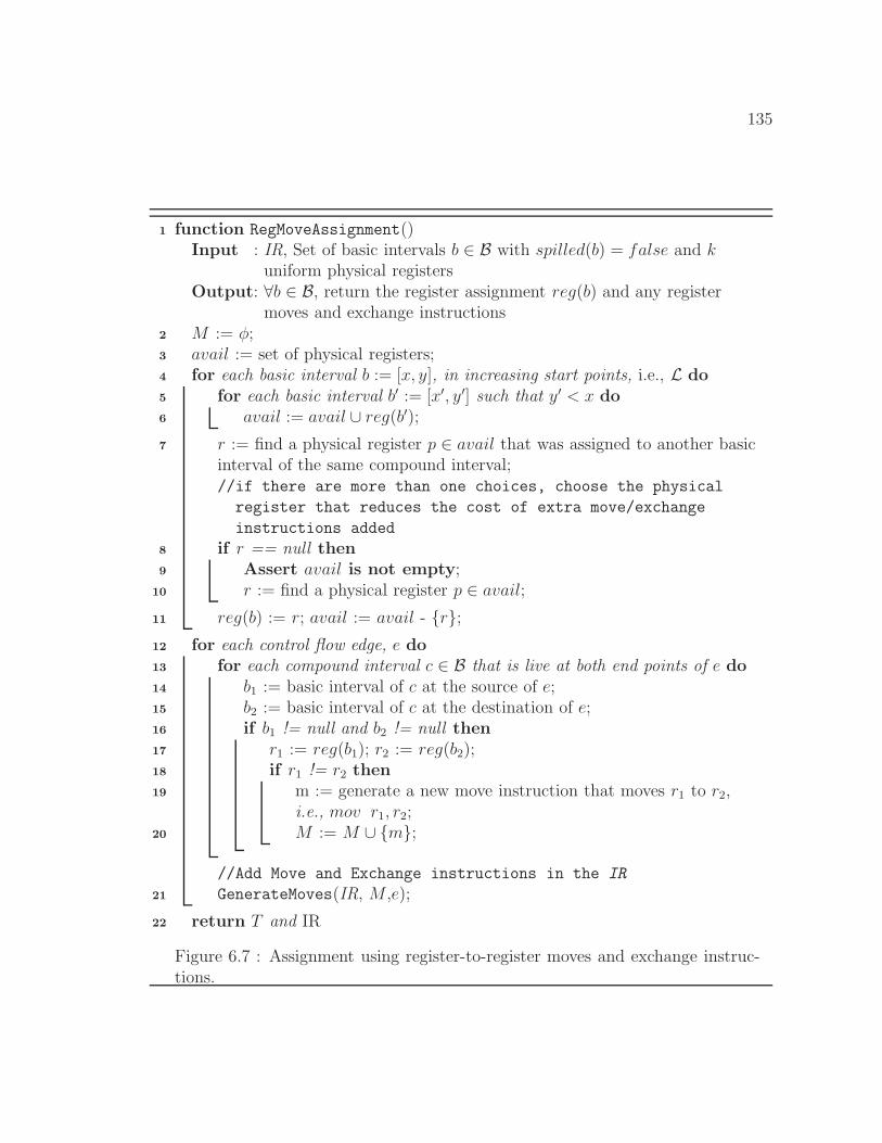
135
function RegMoveAssignment()1
Input : IR, Set of basic intervals b ∈ B with spilled(b) = false and kuniform physical registers
Output: ∀b ∈ B, return the register assignment reg(b) and any registermoves and exchange instructions
M := φ;2
avail := set of physical registers;3
for each basic interval b := [x, y], in increasing start points, i.e., L do4
for each basic interval b′ := [x′, y′] such that y′ < x do5
avail := avail ∪ reg(b′);6
r := find a physical register p ∈ avail that was assigned to another basic7
interval of the same compound interval;//if there are more than one choices, choose the physical
register that reduces the cost of extra move/exchange
instructions added
if r == null then8
Assert avail is not empty;9
r := find a physical register p ∈ avail;10
reg(b) := r; avail := avail - {r};11
for each control flow edge, e do12
for each compound interval c ∈ B that is live at both end points of e do13
b1 := basic interval of c at the source of e;14
b2 := basic interval of c at the destination of e;15
if b1 != null and b2 != null then16
r1 := reg(b1); r2 := reg(b2);17
if r1 != r2 then18
m := generate a new move instruction that moves r1 to r2,19
i.e., mov r1, r2;M := M ∪ {m};20
//Add Move and Exchange instructions in the IR
GenerateMoves(IR, M ,e);21
return T and IR22
Figure 6.7 : Assignment using register-to-register moves and exchange instruc-tions.
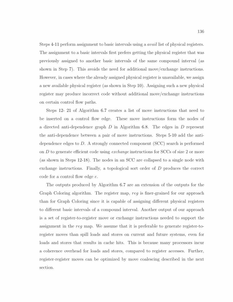
136
Steps 4-11 perform assignment to basic intervals using a avail list of physical registers.
The assignment to a basic intervals first prefers getting the physical register that was
previously assigned to another basic intervals of the same compound interval (as
shown in Step 7). This avoids the need for additional move/exchange instructions.
However, in cases where the already assigned physical register is unavailable, we assign
a new available physical register (as shown in Step 10). Assigning such a new physical
register may produce incorrect code without additional move/exchange instructions
on certain control flow paths.
Steps 12- 21 of Algorithm 6.7 creates a list of move instructions that need to
be inserted on a control flow edge. These move instructions form the nodes of
a directed anti-dependence graph D in Algorithm 6.8. The edges in D represent
the anti-dependence between a pair of move instructions. Steps 5-10 add the anti-
dependence edges to D. A strongly connected component (SCC) search is performed
on D to generate efficient code using exchange instructions for SCCs of size 2 or more
(as shown in Steps 12-18). The nodes in an SCC are collapsed to a single node with
exchange instructions. Finally, a topological sort order of D produces the correct
code for a control flow edge e.
The outputs produced by Algorithm 6.7 are an extension of the outputs for the
Graph Coloring algorithm. The register map, reg is finer-grained for our approach
than for Graph Coloring since it is capable of assigning different physical registers
to different basic intervals of a compound interval. Another output of our approach
is a set of register-to-register move or exchange instructions needed to support the
assignment in the reg map. We assume that it is preferable to generate register-to-
register moves than spill loads and stores on current and future systems, even for
loads and stores that results in cache hits. This is because many processors incur
a coherence overhead for loads and stores, compared to register accesses. Further,
register-register moves can be optimized by move coalescing described in the next
section.
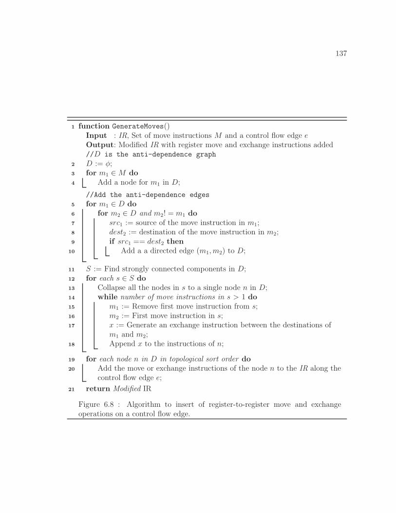
137
function GenerateMoves()1
Input : IR, Set of move instructions M and a control flow edge eOutput: Modified IR with register move and exchange instructions added//D is the anti-dependence graph
D := φ;2
for m1 ∈ M do3
Add a node for m1 in D;4
//Add the anti-dependence edges
for m1 ∈ D do5
for m2 ∈ D and m2! = m1 do6
src1 := source of the move instruction in m1;7
dest2 := destination of the move instruction in m2;8
if src1 == dest2 then9
Add a a directed edge (m1, m2) to D;10
S := Find strongly connected components in D;11
for each s ∈ S do12
Collapse all the nodes in s to a single node n in D;13
while number of move instructions in s > 1 do14
m1 := Remove first move instruction from s;15
m2 := First move instruction in s;16
x := Generate an exchange instruction between the destinations of17
m1 and m2;Append x to the instructions of n;18
for each node n in D in topological sort order do19
Add the move or exchange instructions of the node n to the IR along the20
control flow edge e;
return Modified IR21
Figure 6.8 : Algorithm to insert of register-to-register move and exchangeoperations on a control flow edge.
138
�1
�2
mov r1, r2 mov r2, r1
Figure 6.9 : Anti-dependence graph (D) for example program shown in Figure 6.1.D has a strongly connected component (SCC) which can be reduced to a single nodewith xchg r1, r2 instruction.
6.5.2 Example
Consider our previous example program shown in Figure 6.1. After applying Algo-
rithm 6.7 to the sorted interval start points, we get the following assignments:
reg([1+, 3−]) = r1, reg([2+, 4−]) = r2, reg([4+, 5−]) = r2, reg([3+, 7−]) = r1,
reg([6+, 9−]) = r2, reg([9+, 10−]) = r2, reg([8+, 13−]) = r1, and reg([11+, 14−]) = r2.
We can now observe that along the control-flow edge between statements 4 and 13,
the assignment for compound interval CI(c) changes from r1 to r2. This results in
the creation of a move instruction m1 : mov r1, r2 (due to Step 19 of Algorithm 6.7).
Similarly, along the same control flow edge, the assignment for compound interval
CI(d) changes from r2 to r1. This yields another move instruction m2 : mov r2, r1.
The move instructions m1 and m2 result in an anti-dependence graph D shown
in Figure 6.9. D contains a strongly connected component involving m1 and m2.
We can generate efficient code using exchange instructions according to Steps 11-20
of Algorithm 6.8. The xchg r1, r2 instruction is added along the control-flow edge
between statements 4 and 13.
The example program shown in Figure 6.2 is much simpler. After applying
algorithm 6.7 to the sorted interval start points, we get the following assignments:
reg([1+, 2−]) = r1, reg([2+, 5−]) = r1, reg([4+, 7−]) = r2, reg([6+, 7−]) = r1,
reg([8+, 10−]) = r1, reg([11+, 13−]) = r1, reg([9+, 14−]) = r2, reg([13+, 15−]) = r1,
and reg([14+, 16−]) = r2.
139
This assignment needs a mov r1, r2 instruction to be inserted on the control-flow edge
between statements 7 and 13 as the compound interval CI(d) is switched from r1 to
r2 along that path.
Lemma 6.5.2 The assertion in Step 9 of Algorithm 6.7 never fails.
Proof: Follows from the fact that every interval end point has no more than k sym-
bolic registers simultaneously live. This fact was ensured by the allocation phase.�
Theorem 6.5.3 Given k uniform physical registers, spill-free assignment always finds
an assignment for every b ∈ B whose spilled(b) = false.
Proof: Follows from the previous lemma.�
Theorem 6.5.4 Spill-free assignment takes O(|E| ∗ |C|) space where E represents the
set of control flow edges in a program.
Proof: The additional space requirement in assignment phase is due to the anti-
dependence graph D. For every control-flow edge e ∈ E , in the worst case we need
to insert |C| register-to-register move instructions. These are the number of nodes
in D. The number of edges in D are bounded by the square of the number of
physical registers since it represents all possible anti-dependences between all possible
pairs of physical registers in the worst case. Hence, the overall space complexity is
O(|E| ∗ |C|).�
Theorem 6.5.5 Spill-free assignment takes O(|B| + (|E| ∗ |C|)) time.
Proof: Similar in nature to the proof for Theorem 6.5.4.�
140
6.5.3 Assignment with Move Coalescing and Register Moves
Move coalescing is an important optimization in register-allocation algorithms that as-
sign the same physical register to the source and destination of an IR move instruction
when possible to do so. The register assignment phase must try to coalesce as many
moves as possible so as to get rid of the move instructions from the IR. As we saw
in the preceding section, additional register moves may be inserted in the assignment
phase instead of spilling. In this section we first present a Coalesce Graph that models
both the IR move instructions and register-to-register moves. Then the register
assignment phase on the coalesce graph is formulated as an optimization problem
that tries to maximize the number of move instructions removed after assignment.
Definition 6.5.6 A Coalesce Graph (CG) is an undirected weighted graph, G =
〈V, Em ∪ Er〉, where V represents the basic intervals in B and an edge e ⊆ V × V
corresponds to the following two types of move instructions between a pair of basic
intervals:
1. Em: the move instructions already present in the IR. The weight of such an
edge W(e) is the frequency of the corresponding move instruction.
2. Er: the register-to-register move instructions that need to be added on control-
flow edges for which the two interval end points have different register assign-
ments for the same compound interval. The weight of such an edge W(e) is the
frequency of the control-flow edge on which the move instruction is added. An
exchange instruction can be viewed as consisting of two move instructions.
Definition 6.5.7 Assignment Optimization Problem: Given a set of basic in-
tervals b ∈ B with spilled(b) = false, CG = 〈V, E = {Em ∪Er}〉, IR, and k uniform
physical registers, find a register assignment reg(b) for every basic interval b such that
the following objective function is minimized:
141
∑
∀e∈E, e=(b1,b2) ∧ reg(b1)!=reg(b2)
W(e)
The assignment guides which additional register-to-register copy or exchange instruc-
tions need to be inserted in the IR.
Algorithm 6.10 presents a greedy heuristic to select a physical register for a basic
interval b given the coalesce graph and the available set of physical registers. Map is
a data structure that maps a physical register to a cost. Steps 3-7 find the physical
registers (and their associated costs) that are already assigned to the neighbors of b
in the coalesce graph (similar to the idea of biased coloring [27]). The additional cost
of register-to-register moves that need to be inserted for correct code generation by
assigning a physical register to a basic interval is penalized in Steps 8-11. The greedy
heuristics chooses a physical register reg(b) with maximum cost, i.e., the benefit of
assigning the physical register to basic interval b.
Theorem 6.5.8 Register assignment using Algorithm 6.10 requires O(|B| + |IR| +
(|C| ∗ maxc)) space where maxc denotes the maximum number of basic intervals that
a compound interval has.
Proof: The additional space requirement is due to the coalesce graph CG containing
|B| number of nodes. Em in the worst case ends up creating |IR| edges. Er adds edges
between basic intervals of the same compound interval and hence needs |C| ∗ maxc
number of edges.�
Theorem 6.5.9 Register assignment using Algorithm 6.10 takes O((|B| ∗ maxc) +
|IR| + (|E| ∗ |C|)) time.
Proof: In addition to Theorem 6.5.5, before deciding a physical register for each basic
interval b it is required to traverse each of the neighbors in CG. For all basic intervals,
this adds over all |IR| time complexity for IR move instructions and |B| ∗ maxc time
complexity for Er edges in CG.�
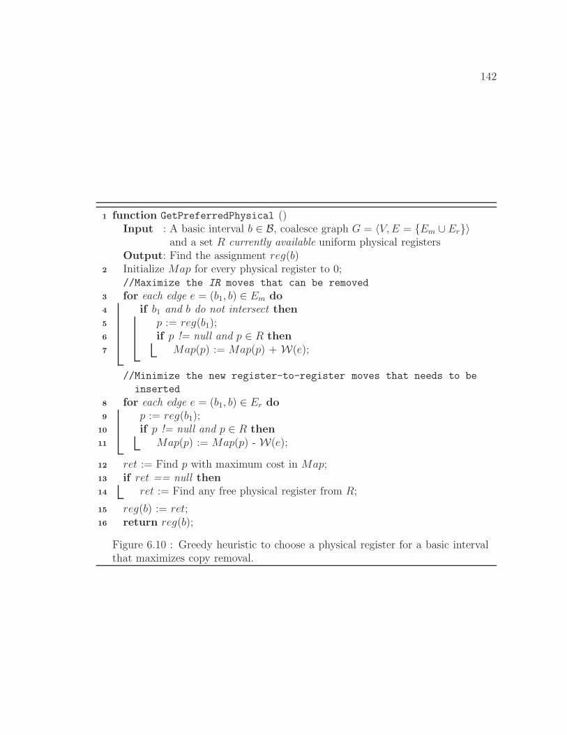
142
function GetPreferredPhysical ()1
Input : A basic interval b ∈ B, coalesce graph G = 〈V, E = {Em ∪ Er}〉and a set R currently available uniform physical registers
Output: Find the assignment reg(b)Initialize Map for every physical register to 0;2
//Maximize the IR moves that can be removed
for each edge e = (b1, b) ∈ Em do3
if b1 and b do not intersect then4
p := reg(b1);5
if p != null and p ∈ R then6
Map(p) := Map(p) + W(e);7
//Minimize the new register-to-register moves that needs to be
inserted
for each edge e = (b1, b) ∈ Er do8
p := reg(b1);9
if p != null and p ∈ R then10
Map(p) := Map(p) - W(e);11
ret := Find p with maximum cost in Map;12
if ret == null then13
ret := Find any free physical register from R;14
reg(b) := ret;15
return reg(b);16
Figure 6.10 : Greedy heuristic to choose a physical register for a basic intervalthat maximizes copy removal.
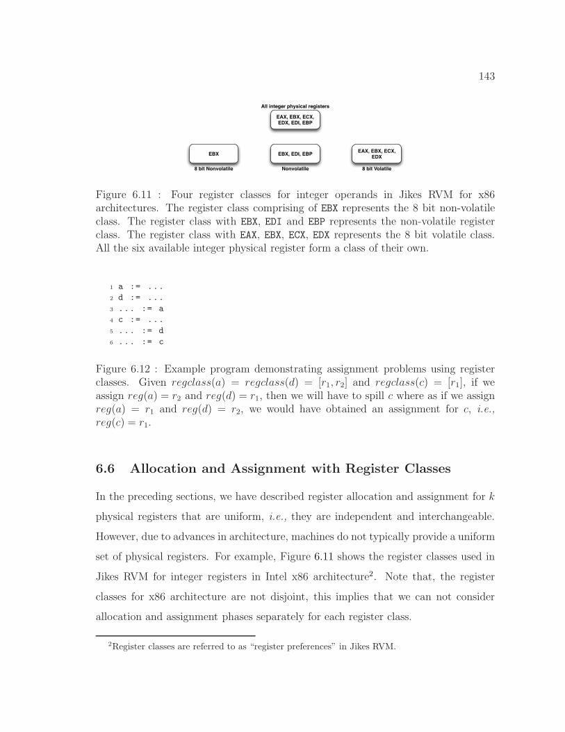
143
EBX EBX, EDI, EBPEAX, EBX, ECX,
EDX
EAX, EBX, ECX, EDX, EDI, EBP
8 bit Nonvolatile Nonvolatile 8 bit Volatile
All integer physical registers
Figure 6.11 : Four register classes for integer operands in Jikes RVM for x86architectures. The register class comprising of EBX represents the 8 bit non-volatileclass. The register class with EBX, EDI and EBP represents the non-volatile registerclass. The register class with EAX, EBX, ECX, EDX represents the 8 bit volatile class.All the six available integer physical register form a class of their own.
1 a := ...
2 d := ...
3 ... := a
4 c := ...
5 ... := d
6 ... := c
Figure 6.12 : Example program demonstrating assignment problems using registerclasses. Given regclass(a) = regclass(d) = [r1, r2] and regclass(c) = [r1], if weassign reg(a) = r2 and reg(d) = r1, then we will have to spill c where as if we assignreg(a) = r1 and reg(d) = r2, we would have obtained an assignment for c, i.e.,reg(c) = r1.
6.6 Allocation and Assignment with Register Classes
In the preceding sections, we have described register allocation and assignment for k
physical registers that are uniform, i.e., they are independent and interchangeable.
However, due to advances in architecture, machines do not typically provide a uniform
set of physical registers. For example, Figure 6.11 shows the register classes used in
Jikes RVM for integer registers in Intel x86 architecture2. Note that, the register
classes for x86 architecture are not disjoint, this implies that we can not consider
allocation and assignment phases separately for each register class.
2Register classes are referred to as “register preferences” in Jikes RVM.
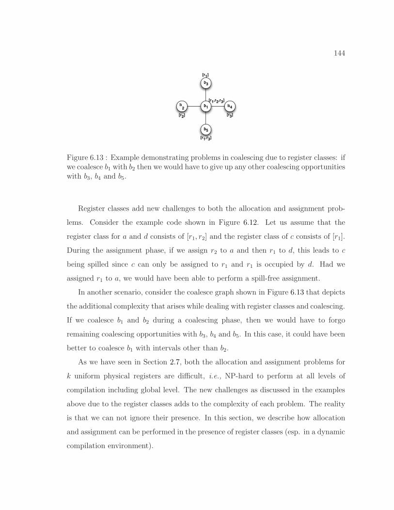
144
�1
�2
�3
�5
�4
[r2]
[r1,r3]
[r3]
[r1]
[r1,r2,r3]
Figure 6.13 : Example demonstrating problems in coalescing due to register classes: ifwe coalesce b1 with b2 then we would have to give up any other coalescing opportunitieswith b3, b4 and b5.
Register classes add new challenges to both the allocation and assignment prob-
lems. Consider the example code shown in Figure 6.12. Let us assume that the
register class for a and d consists of [r1, r2] and the register class of c consists of [r1].
During the assignment phase, if we assign r2 to a and then r1 to d, this leads to c
being spilled since c can only be assigned to r1 and r1 is occupied by d. Had we
assigned r1 to a, we would have been able to perform a spill-free assignment.
In another scenario, consider the coalesce graph shown in Figure 6.13 that depicts
the additional complexity that arises while dealing with register classes and coalescing.
If we coalesce b1 and b2 during a coalescing phase, then we would have to forgo
remaining coalescing opportunities with b3, b4 and b5. In this case, it could have been
better to coalesce b1 with intervals other than b2.
As we have seen in Section 2.7, both the allocation and assignment problems for
k uniform physical registers are difficult, i.e., NP-hard to perform at all levels of
compilation including global level. The new challenges as discussed in the examples
above due to the register classes adds to the complexity of each problem. The reality
is that we can not ignore their presence. In this section, we describe how allocation
and assignment can be performed in the presence of register classes (esp. in a dynamic
compilation environment).
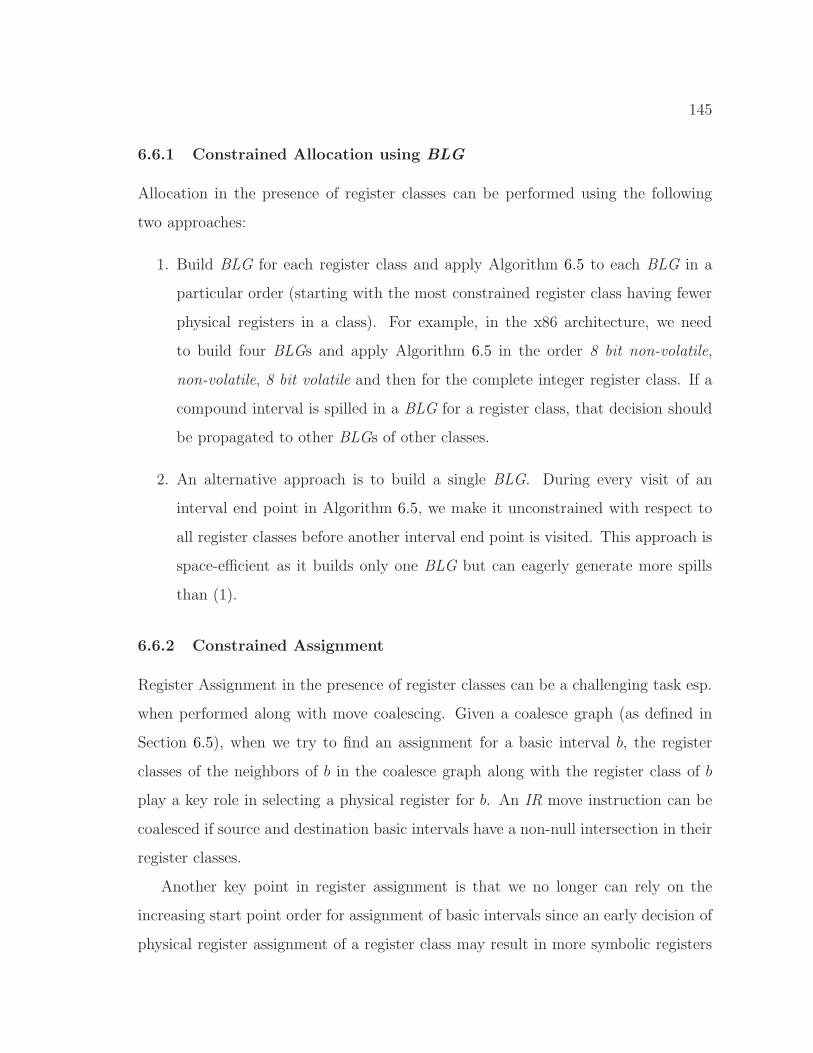
145
6.6.1 Constrained Allocation using BLG
Allocation in the presence of register classes can be performed using the following
two approaches:
1. Build BLG for each register class and apply Algorithm 6.5 to each BLG in a
particular order (starting with the most constrained register class having fewer
physical registers in a class). For example, in the x86 architecture, we need
to build four BLGs and apply Algorithm 6.5 in the order 8 bit non-volatile,
non-volatile, 8 bit volatile and then for the complete integer register class. If a
compound interval is spilled in a BLG for a register class, that decision should
be propagated to other BLGs of other classes.
2. An alternative approach is to build a single BLG. During every visit of an
interval end point in Algorithm 6.5, we make it unconstrained with respect to
all register classes before another interval end point is visited. This approach is
space-efficient as it builds only one BLG but can eagerly generate more spills
than (1).
6.6.2 Constrained Assignment
Register Assignment in the presence of register classes can be a challenging task esp.
when performed along with move coalescing. Given a coalesce graph (as defined in
Section 6.5), when we try to find an assignment for a basic interval b, the register
classes of the neighbors of b in the coalesce graph along with the register class of b
play a key role in selecting a physical register for b. An IR move instruction can be
coalesced if source and destination basic intervals have a non-null intersection in their
register classes.
Another key point in register assignment is that we no longer can rely on the
increasing start point order for assignment of basic intervals since an early decision of
physical register assignment of a register class may result in more symbolic registers
146
being spilled later on or giving up other opportunities for coalescing (as shown in
Figure 6.12).
Definition 6.6.1 Constrained Assignment Optimization Problem: Given a
set of basic intervals b ∈ B with spilled(b) = false, regclass(b) indicating physical
registers that can be assigned to each b, CG = 〈V, E = {Em ∪ Er}〉, and IR, find a
register assignment reg(b) for a subset of basic intervals S ⊆ B such that the following
objective function is minimized:
∑
∀b∈B−S
SPILL(b) +∑
∀e∈E, e=(b1,b2) ∧ reg(b1)!=reg(b2)
W(e)
Insert additional register-to-register copy or exchange instructions in the IR.
Algorithm 6.14 presents a bucket-based approach to register assignment that tries
to strike a balance between register classes and spill cost. The toColor is a data
structure that holds sorted basic intervals according to register classes in a two
dimensional array. Steps 8-13 fill in elements of toColor array in the next available
bucket. Steps 14-17 find an assignment for basic intervals by traversing the toColor
array in row major order.
Algorithm 6.15 describes a heuristic for selecting an assignment for a basic interval.
Steps 6-14 compute costs for physical registers that are already assigned to neighbors
and that are not yet assigned to neighbors but will be assigned in future. The reason
we consider the unassigned neighbors is to avoid eager decisions of move coalescing.
Steps 15-18 penalize the cost of additional register-to-register moves inserted on
control flow edges. Finally, Steps 19-21 find a physical register if one is available.
Steps 22-24, spills the basic interval if there is no physical register available.
The space and time requirement of Algorithm 6.14 is similar to those of Algo-
rithm 6.10.
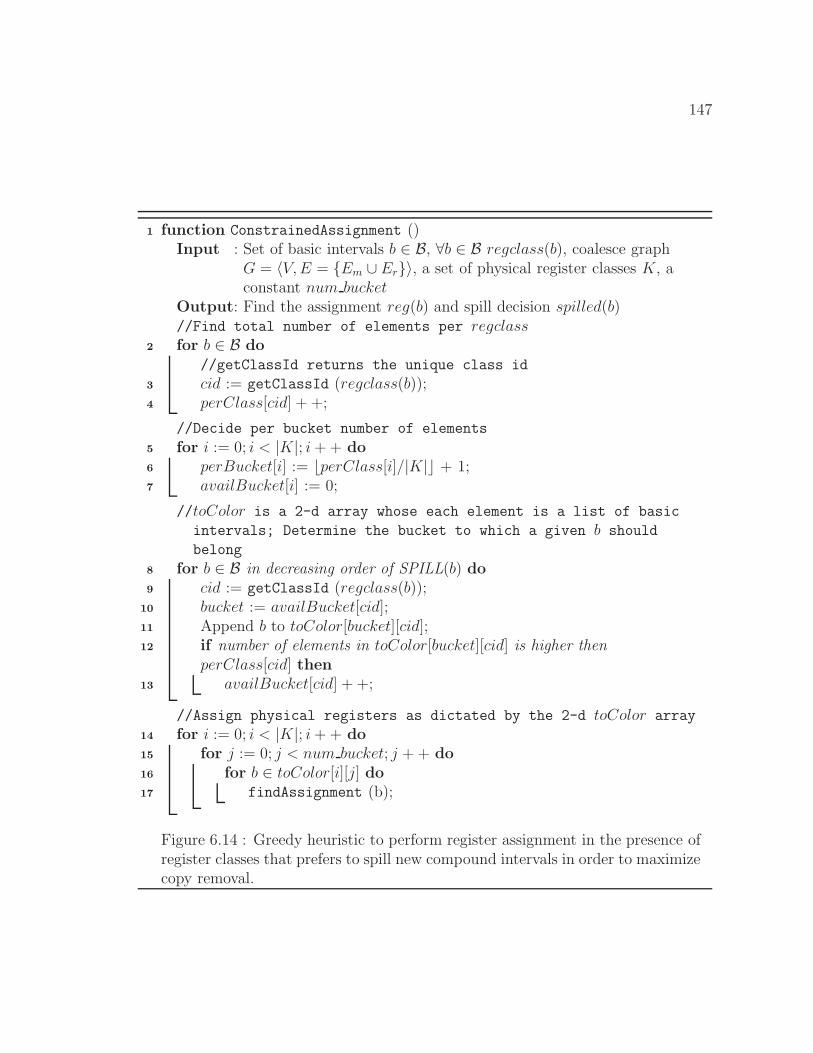
147
function ConstrainedAssignment ()1
Input : Set of basic intervals b ∈ B, ∀b ∈ B regclass(b), coalesce graphG = 〈V, E = {Em ∪ Er}〉, a set of physical register classes K, aconstant num bucket
Output: Find the assignment reg(b) and spill decision spilled(b)//Find total number of elements per regclassfor b ∈ B do2
//getClassId returns the unique class id
cid := getClassId (regclass(b));3
perClass[cid] + +;4
//Decide per bucket number of elements
for i := 0; i < |K|; i + + do5
perBucket[i] := ⌊perClass[i]/|K|⌋ + 1;6
availBucket[i] := 0;7
//toColor is a 2-d array whose each element is a list of basic
intervals; Determine the bucket to which a given b should
belong
for b ∈ B in decreasing order of SPILL(b) do8
cid := getClassId (regclass(b));9
bucket := availBucket[cid];10
Append b to toColor[bucket][cid];11
if number of elements in toColor[bucket][cid] is higher then12
perClass[cid] thenavailBucket[cid] + +;13
//Assign physical registers as dictated by the 2-d toColor array
for i := 0; i < |K|; i + + do14
for j := 0; j < num bucket; j + + do15
for b ∈ toColor[i][j] do16
findAssignment (b);17
Figure 6.14 : Greedy heuristic to perform register assignment in the presence ofregister classes that prefers to spill new compound intervals in order to maximizecopy removal.
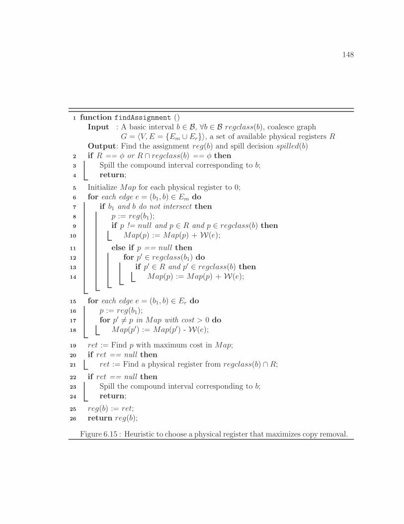
148
function findAssignment ()1
Input : A basic interval b ∈ B, ∀b ∈ B regclass(b), coalesce graphG = 〈V, E = {Em ∪ Er}〉, a set of available physical registers R
Output: Find the assignment reg(b) and spill decision spilled(b)if R == φ or R ∩ regclass(b) == φ then2
Spill the compound interval corresponding to b;3
return;4
Initialize Map for each physical register to 0;5
for each edge e = (b1, b) ∈ Em do6
if b1 and b do not intersect then7
p := reg(b1);8
if p != null and p ∈ R and p ∈ regclass(b) then9
Map(p) := Map(p) + W(e);10
else if p == null then11
for p′ ∈ regclass(b1) do12
if p′ ∈ R and p′ ∈ regclass(b) then13
Map(p) := Map(p) + W(e);14
for each edge e = (b1, b) ∈ Er do15
p := reg(b1);16
for p′ 6= p in Map with cost > 0 do17
Map(p′) := Map(p′) - W(e);18
ret := Find p with maximum cost in Map;19
if ret == null then20
ret := Find a physical register from regclass(b) ∩ R;21
if ret == null then22
Spill the compound interval corresponding to b;23
return;24
reg(b) := ret;25
return reg(b);26
Figure 6.15 : Heuristic to choose a physical register that maximizes copy removal.
149
6.7 Extended Linear Scan (ELS)
In the preceding sections, we have described space-efficient register allocation using
the Bipartite Liveness Graph. In this section, we will describe an Extended Linear
Scan (ELS) register allocation algorithm that uses even less space than a space-
efficient register allocation algorithm. The key point addressed in the Extended Linear
Scan is that it does not need an explicit representation for the Bipartite Liveness
Graph, but uses numlive information at interval end points.
Figure 6.16 summarizes our Extended Linear Scan algorithm. Steps 3-8 are the
Potential Spill pass. We use the observation that the only interval end points p for
which spill decisions need to be made are those for which numlive[p] > k. The
heuristic used in Step 4 is to process these interval end points in decreasing order of
FREQ[q]. As in Chaitin’s Graph Coloring algorithm, Step 5 selects the compound
interval with the smallest spillcost for spilling. A key difference with graph coloring
is that this decision is driven by the choice of interval end point p, and allows for
assigning different physical registers to the same symbolic register at different program
points. After Step 3 has completed, a feasible register allocation is obtained with
numlive[p] ≤ k at each interval end point p. The set of compound intervals selected
to be spilled are identified by spilled(s) = true, and are also pushed onto stack
S. Steps 9-14 is the Actual Spill pass. It examines the compound intervals pushed
on the stack to see if any of them can be “unspilled”. Step 15 is the Select pass.
The algorithm for register assignment with register-to-register move and exchange
instructions is already discussed in Section 6.5.3.
Theorem 6.7.1 The ELS algorithm takes O(|B|+|C|) space and O(|B|+|B|(log(maxc)+
log|B|)) time, where maxc is the maximum value of numlive[p] at any interval end
point p.
Proof: For Step 3 (Potential Spill), the selection in Step 4 of program point q with
numlive[q] > k and largest estimated frequency, FREQ[q], contributes O(|B|log|B|)
150
time and Step 5 contributes O(|B|log(maxc)) time, assuming that a heap data struc-
ture (or equivalent) is used in both cases. Finally, Step 9 (Actual Spill) and Step 15
(Register Assignment) contribute at most O(|B|) time. �.
6.8 Summary
In this chapter, we addressed the problem of compile time and space efficient register
allocation. Most approaches to register allocation involve the construction of an
interference graph, which is known from past work to be a major space and time
bottleneck [42, 105]. A notable exception is the Linear Scan algorithm which is
favored by many dynamic and just-in-time compilers because it avoids the overhead
of constructing an interference graph. We introduced a new approach to register allo-
cation that improves on the runtime performance delivered by Linear Scan, without
exceeding its space bound. To that end, we introduced a Bipartite Liveness Graph
representation as an alternative foundation to the interference graph. Allocation
with the BLG is formulated as an optimization problem and a greedy heuristic is
presented to solve it. We also formulated spill-free register assignment combined with
move coalescing as a combined optimization problem using the Coalesce Graph, which
models both IR move instructions and additional register-to-register moves/exchanges
arising from register assignment. We then extended the above register allocation and
assignment approaches to handle register classes. Experimental evaluation of our
proposed allocator is provided in Section 8.2.
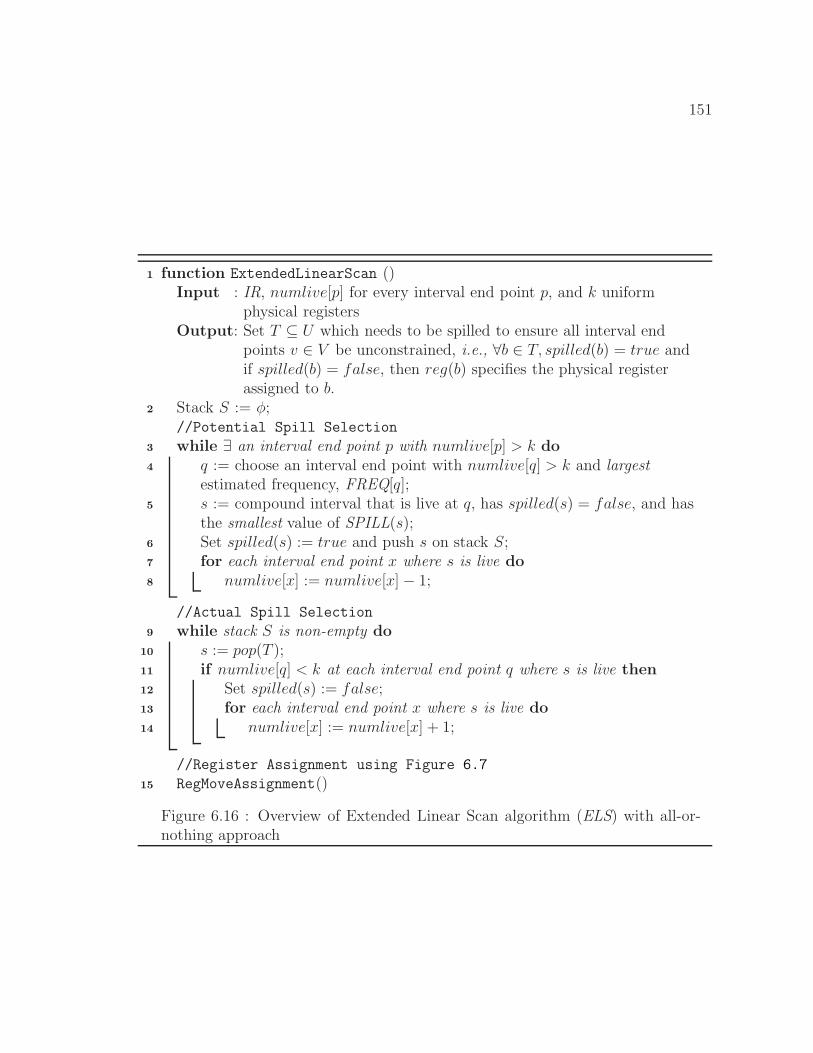
151
function ExtendedLinearScan ()1
Input : IR, numlive[p] for every interval end point p, and k uniformphysical registers
Output: Set T ⊆ U which needs to be spilled to ensure all interval endpoints v ∈ V be unconstrained, i.e., ∀b ∈ T, spilled(b) = true andif spilled(b) = false, then reg(b) specifies the physical registerassigned to b.
Stack S := φ;2
//Potential Spill Selection
while ∃ an interval end point p with numlive[p] > k do3
q := choose an interval end point with numlive[q] > k and largest4
estimated frequency, FREQ[q];s := compound interval that is live at q, has spilled(s) = false, and has5
the smallest value of SPILL(s);Set spilled(s) := true and push s on stack S;6
for each interval end point x where s is live do7
numlive[x] := numlive[x] − 1;8
//Actual Spill Selection
while stack S is non-empty do9
s := pop(T );10
if numlive[q] < k at each interval end point q where s is live then11
Set spilled(s) := false;12
for each interval end point x where s is live do13
numlive[x] := numlive[x] + 1;14
//Register Assignment using Figure 6.7
RegMoveAssignment()15
Figure 6.16 : Overview of Extended Linear Scan algorithm (ELS) with all-or-nothing approach

152
Chapter 7
Bitwidth-aware Register Allocation
Bitwidth-aware Register allocation [116] extends the traditional register allocators by
packing subword data values, i.e., data values with narrower width than the standard
data width (word size) supported by the underlying processor. The packed data
values can be allocated in the same physical register, thereby moderating the register
pressure of the program. Various applications, in particular from the embedded
domain, make extensive use of sub-word sized values and can benefit significantly
by bitwidth-aware register allocation.
In this chapter, we propose three key contributions to bitwidth-aware register
allocation: 1) a limit study that compares the Tallam-Gupta bitwidth analysis algo-
rithm [116] with a dynamic profile-driven bitwidth information, and show significant
opportunities for enhancements; 2) an enhanced bitwidth analysis algorithm that
performs more detailed scalar and array analysis for improved bitwidth information
than in Tallam-Gupta; 3) an enhanced packing algorithm that improves packing
algorithm of Tallam-Gupta by a new set of safe bitwidth estimates.
Bitwidth
AnalysisBuild IG
Variable
Packing
Move
Insertion
Register
Allocation
Figure 7.1 : Overall Bitwidth-aware register allocation framework.
153
7.1 Overall Bitwidth-aware register allocation
Figure 7.1 depicts the overall flow of a bitwidth-aware register allocation algorithm.
The core of a bitwidth-aware register allocation lies in the bitwidth analysis that
computes actual width requirements for every variable at every program point. This
bitwidth information is used to annotate the edges of the interference graph during
the Build phase. Iterative Packing is then applied over the interference graph to
pack narrow width live ranges as long as they can be packed onto the same physical
register. Additional move instructions are added in the IR for extracting individual
variables from the packed variables and finally, the global register allocation algorithm
is applied for the variables that includes the new packed variables created in Packing
step.
7.2 Limit Study
Our first step in studying bitwidth-aware register allocation was to perform a limit
study that compares the bitwidth usage computed by the static compile-time bitwidth
analysis algorithm in Tallam-Gupta (also described in Section 2.8.1) with dynamic
bitwidth information obtained from an execution profile. The infrastructure used for
this study was based on the GCC compiler, as depicted in Figure 7.2. The register
allocation phase in GCC was modified to accept input from the box labeled “Bitwidth
Analysis”, which can either generate compile-time or profile-driven bitwidth informa-
tion. Using Tallam-Gupta bitwidth analysis, the width of a variable at a program
point can be represented by three parts: a leading part of unused bits (l), a middle part
of active bits, and a trailing part of unused bits (t). We implemented the Tallam-
Gupta bitwidth algorithm in the GCC compiler to obtain this information for the
compile-time case. For the profile-driven case, we instrumented the code generated
by GCC so as to perform a “logical or” of the values dynamically assigned to each
variable. The major motivation for performing the limit study is that the prior work
by Tallam-Gupta reported static benefits of bitwidth-aware register allocation (fewer

154
bitwidth
RTL
C Program
Bitwidth analysis
analysis
Register allocation
Other Backend phases
Executable code
Program Execution
Compile time Profile−drivenbitwidth info
Backend phases
GCC Frontend
Profile Info
Figure 7.2 : GCC modification for Limit Study
registers used, smaller cliques in the interference graph), but did not provide any
indication of what additional opportunities remain for improved bitwidth analysis.
The benchmarks used in our evaluation were all taken from the Bitwise benchmark
set [17], so as to be representative of embedded applications. Our evaluation was
performed on 9 out of the 15 programs in the full benchmark set. The following
five programs were not used because they did not contain a return value, thereby
making it possible for GCC to optimize away the entire program as dead code —
bilint, levdurb, motiontest, sha, softfloat. In addition, the life program was not used,
because the Bitwise benchmark set already contains a newlife program which is very
similar to life. All experiments were performed using the -O3 option and the –param
max-unroll-times=0 option1 with version 4.1 of GCC targeted to the x86 platform.
Table 7.1 lists the total number of variables (symbolic registers) available for
1This option disables loop unrolling. Loop unrolling can create more candidates for registerallocation, but the relative impact of unrolling depends on the benchmark so it was disabled.
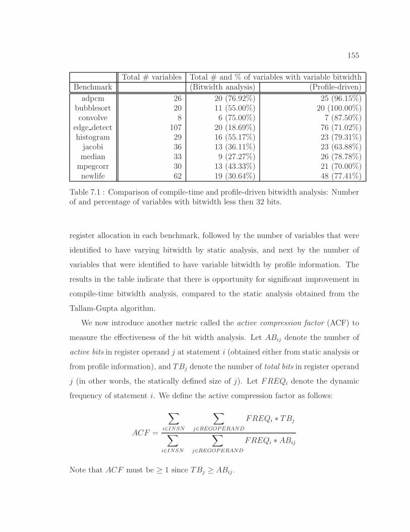
155
Total # variables Total # and % of variables with variable bitwidthBenchmark (Bitwidth analysis) (Profile-driven)
adpcm 26 20 (76.92%) 25 (96.15%)bubblesort 20 11 (55.00%) 20 (100.00%)convolve 8 6 (75.00%) 7 (87.50%)
edge detect 107 20 (18.69%) 76 (71.02%)histogram 29 16 (55.17%) 23 (79.31%)
jacobi 36 13 (36.11%) 23 (63.88%)median 33 9 (27.27%) 26 (78.78%)
mpegcorr 30 13 (43.33%) 21 (70.00%)newlife 62 19 (30.64%) 48 (77.41%)
Table 7.1 : Comparison of compile-time and profile-driven bitwidth analysis: Numberof and percentage of variables with bitwidth less then 32 bits.
register allocation in each benchmark, followed by the number of variables that were
identified to have varying bitwidth by static analysis, and next by the number of
variables that were identified to have variable bitwidth by profile information. The
results in the table indicate that there is opportunity for significant improvement in
compile-time bitwidth analysis, compared to the static analysis obtained from the
Tallam-Gupta algorithm.
We now introduce another metric called the active compression factor (ACF) to
measure the effectiveness of the bit width analysis. Let ABij denote the number of
active bits in register operand j at statement i (obtained either from static analysis or
from profile information), and TBj denote the number of total bits in register operand
j (in other words, the statically defined size of j). Let FREQi denote the dynamic
frequency of statement i. We define the active compression factor as follows:
ACF =
∑
i∈INSN
∑
j∈REGOPERAND
FREQi ∗ TBj
∑
i∈INSN
∑
j∈REGOPERAND
FREQi ∗ ABij
Note that ACF must be ≥ 1 since TBj ≥ ABij .
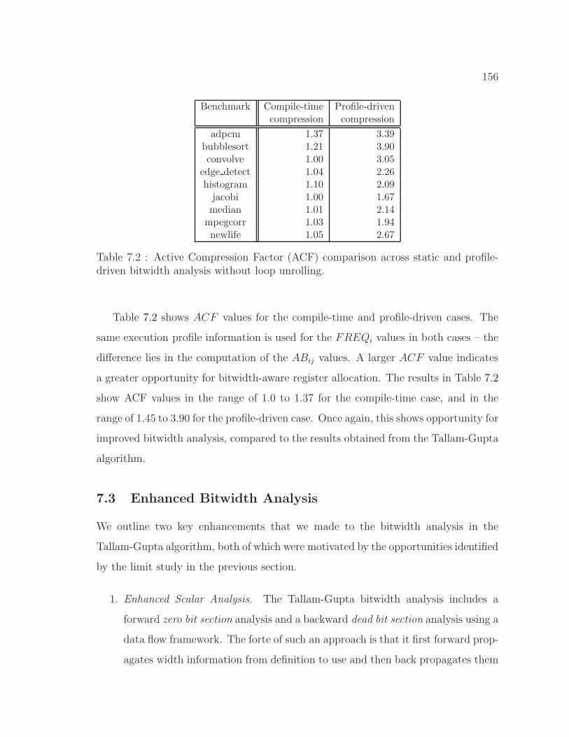
156
Benchmark Compile-time Profile-drivencompression compression
adpcm 1.37 3.39bubblesort 1.21 3.90convolve 1.00 3.05
edge detect 1.04 2.26histogram 1.10 2.09
jacobi 1.00 1.67median 1.01 2.14
mpegcorr 1.03 1.94newlife 1.05 2.67
Table 7.2 : Active Compression Factor (ACF) comparison across static and profile-driven bitwidth analysis without loop unrolling.
Table 7.2 shows ACF values for the compile-time and profile-driven cases. The
same execution profile information is used for the FREQi values in both cases – the
difference lies in the computation of the ABij values. A larger ACF value indicates
a greater opportunity for bitwidth-aware register allocation. The results in Table 7.2
show ACF values in the range of 1.0 to 1.37 for the compile-time case, and in the
range of 1.45 to 3.90 for the profile-driven case. Once again, this shows opportunity for
improved bitwidth analysis, compared to the results obtained from the Tallam-Gupta
algorithm.
7.3 Enhanced Bitwidth Analysis
We outline two key enhancements that we made to the bitwidth analysis in the
Tallam-Gupta algorithm, both of which were motivated by the opportunities identified
by the limit study in the previous section.
1. Enhanced Scalar Analysis. The Tallam-Gupta bitwidth analysis includes a
forward zero bit section analysis and a backward dead bit section analysis using a
data flow framework. The forte of such an approach is that it first forward prop-
agates width information from definition to use and then back propagates them
157
from use to definition. Although their approach analyzed variables involved in
logical operations efficiently, they did not compute accurate width information
for variables involved in operations such as arithmetic computations. Consider
the programming scenario where a variable is incremented inside a loop by some
constant value. If we knew the loop bounds, we can compute the upper bound
on the value that can be assigned to the variable. This can be used to decide
the useful bits of the variable. This kind of programming scenario is seen very
often in Bitwise benchmark set [17].
Bitwidth analysis for variables modified inside loops require a closed-form so-
lution. We extended the bitwidth analysis of Tallam-Gupta with a recurrence
analysis that can identify general induction variables and other patterns with
closed-form solutions. This is more general than the scalar range analysis
presented by [115].
Each closed form expression for a variable x updated inside a loop-nest is
represented using a linear chrec that is expressed using {base, op, stride} and
is evaluated using Newton’s interpolation formula as {base, +, stride}(x) :=
base + step ∗ x. The base represents the value computed outside the loop nest
and the stride represents the value added or subtracted in every iteration of the
loop. Note that the stride can also be a variable whose bitwidth information
is already available or whose closed-form expression can be/is being computed.
The idea of using chrec representation is that it can be evaluated quickly using
Newton’s interpolation formula. Note that the recurrence analysis can analyze
improper loop nests.
Given chrec representation for each statement of a loop nest l, the high level
algorithm to compute the range of possible values for variables defined in l
using SSA-based intermediate representation is provided in [15]. Typically an
SSA based intermediate representation is unavailable during register allocation
level. We present a recurrence analysis using the Program Dependence Graph

158
(PDG). The steps are provided in Algorithm 7.3. A cycle in the PDG represents
the need for a closed-form solution. Since each statement in the PDG has an
associated chrec, we combine multiple chrecs of the statements in the PDG. The
combined chrecs can then be evaluated using Newton’s interpolation formula
given the base value and the loop bounds.
2. Enhanced Array Analysis. A key limitation of the Tallam-Gupta algorithm
is that it performs no analysis of array variables. We added an array range
analysis that tracks the values being assigned to arrays, and integrates the
array analysis with the enhanced scalar analysis. This enhancement performs
a flow-insensitive analysis of all accesses to an array variable.
function RecurrenceAnalysis ()1
Input : IR, loop nest lOutput: Width of the variables defined inside loop nest lPerform renaming in the IR;2
Compute the Program Dependence Graph (PDG);3
for each SCC in PDG do4
Combine the chrecs of the statements in the SCC;5
Collapse the SCC into a single node in the PDG;6
Perform a topological sort of nodes in the PDG and propagate the chrecs;7
Using the upper and lower bounds of l and the initial values of variables8
outside l, evaluate the combined chrecs;
Figure 7.3 : Recurrence analysis for computing bitwidth information of variablesaccessed inside loops.
We use two code examples to illustrate the benefits of these two enhancements,
and how they are used in conjunction with each other. Figure 7.4 contains a code
fragment from the Bitwise adpcm benchmark. While it may not be standard practice
in general, it is common practice in embedded applications for loop iterations to
be bounded by compile-time constants defined in the program. When analyzing the
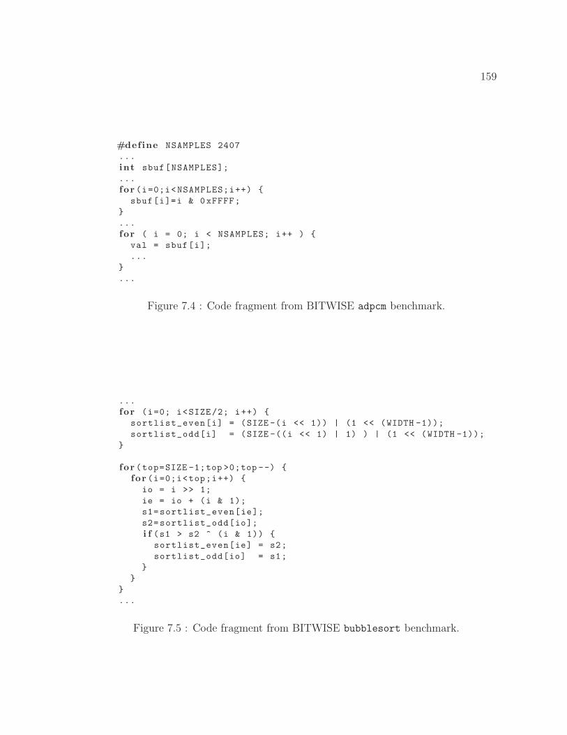
159
#define NSAMPLES 2407
...
int sbuf[NSAMPLES];
...
for (i=0;i<NSAMPLES;i++) {
sbuf[i]=i & 0xFFFF;
}
...
for ( i = 0; i < NSAMPLES; i++ ) {
val = sbuf[i];
...
}
...
Figure 7.4 : Code fragment from BITWISE adpcm benchmark.
...
for (i=0; i<SIZE/2; i++) {
sortlist_even[i] = (SIZE -(i << 1)) | (1 << (WIDTH -1));
sortlist_odd[i] = (SIZE -((i << 1) | 1) ) | (1 << (WIDTH -1));
}
for (top=SIZE -1;top >0;top --) {
for (i=0;i<top;i++) {
io = i >> 1;
ie = io + (i & 1);
s1=sortlist_even[ie];
s2=sortlist_odd[io];
i f (s1 > s2 ^ (i & 1)) {
sortlist_even[ie] = s2;
sortlist_odd[io] = s1;
}
}
}
...
Figure 7.5 : Code fragment from BITWISE bubblesort benchmark.
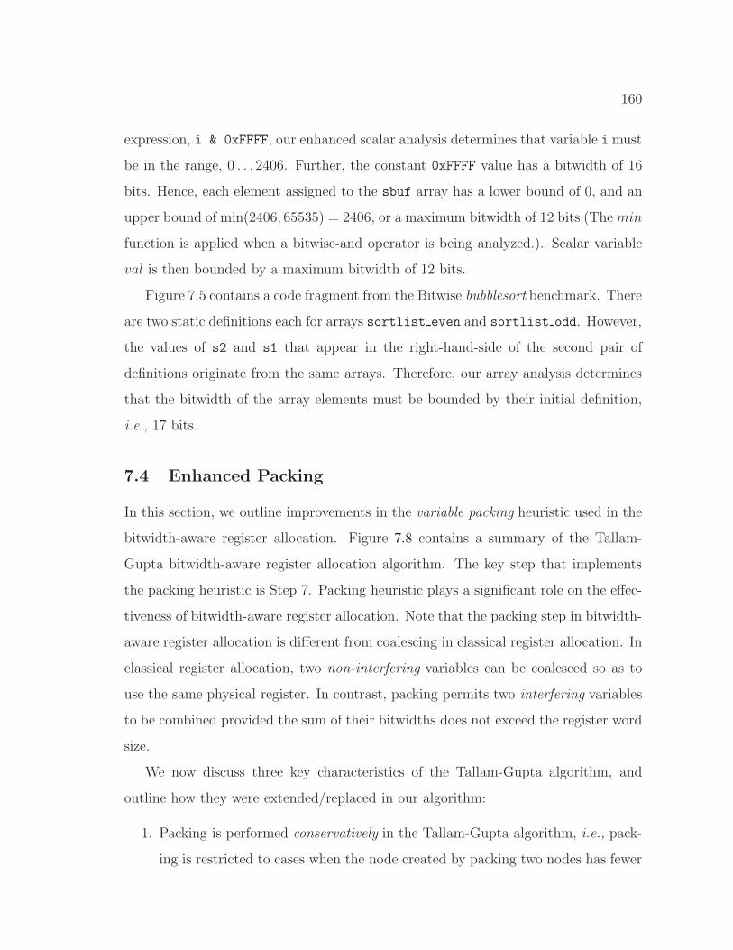
160
expression, i & 0xFFFF, our enhanced scalar analysis determines that variable i must
be in the range, 0 . . . 2406. Further, the constant 0xFFFF value has a bitwidth of 16
bits. Hence, each element assigned to the sbuf array has a lower bound of 0, and an
upper bound of min(2406, 65535) = 2406, or a maximum bitwidth of 12 bits (The min
function is applied when a bitwise-and operator is being analyzed.). Scalar variable
val is then bounded by a maximum bitwidth of 12 bits.
Figure 7.5 contains a code fragment from the Bitwise bubblesort benchmark. There
are two static definitions each for arrays sortlist even and sortlist odd. However,
the values of s2 and s1 that appear in the right-hand-side of the second pair of
definitions originate from the same arrays. Therefore, our array analysis determines
that the bitwidth of the array elements must be bounded by their initial definition,
i.e., 17 bits.
7.4 Enhanced Packing
In this section, we outline improvements in the variable packing heuristic used in the
bitwidth-aware register allocation. Figure 7.8 contains a summary of the Tallam-
Gupta bitwidth-aware register allocation algorithm. The key step that implements
the packing heuristic is Step 7. Packing heuristic plays a significant role on the effec-
tiveness of bitwidth-aware register allocation. Note that the packing step in bitwidth-
aware register allocation is different from coalescing in classical register allocation. In
classical register allocation, two non-interfering variables can be coalesced so as to
use the same physical register. In contrast, packing permits two interfering variables
to be combined provided the sum of their bitwidths does not exceed the register word
size.
We now discuss three key characteristics of the Tallam-Gupta algorithm, and
outline how they were extended/replaced in our algorithm:
1. Packing is performed conservatively in the Tallam-Gupta algorithm, i.e., pack-
ing is restricted to cases when the node created by packing two nodes has fewer
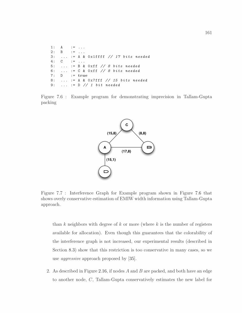
161
1: A := ...
2: B := ...
3: ... := A & 0x1ffff // 17 bits needed
4: C := ...
5: ... := B & 0xff // 8 bits needed
6: ... := C & 0xff // 8 bits needed
7: D := true
8: ... := A & 0x7fff // 15 bits needed
9: ... := D // 1 bit needed
Figure 7.6 : Example program for demonstrating imprecision in Tallam-Guptapacking �
A B
(15,8)
(17,8)
(8,8)
D
(15,1)
Figure 7.7 : Interference Graph for Example program shown in Figure 7.6 thatshows overly conservative estimation of EMIW width information using Tallam-Guptaapproach.
than k neighbors with degree of k or more (where k is the number of registers
available for allocation). Even though this guarantees that the colorability of
the interference graph is not increased, our experimental results (described in
Section 8.3) show that this restriction is too conservative in many cases, so we
use aggressive approach proposed by [35].
2. As described in Figure 2.16, if nodes A and B are packed, and both have an edge
to another node, C, Tallam-Gupta conservatively estimates the new label for
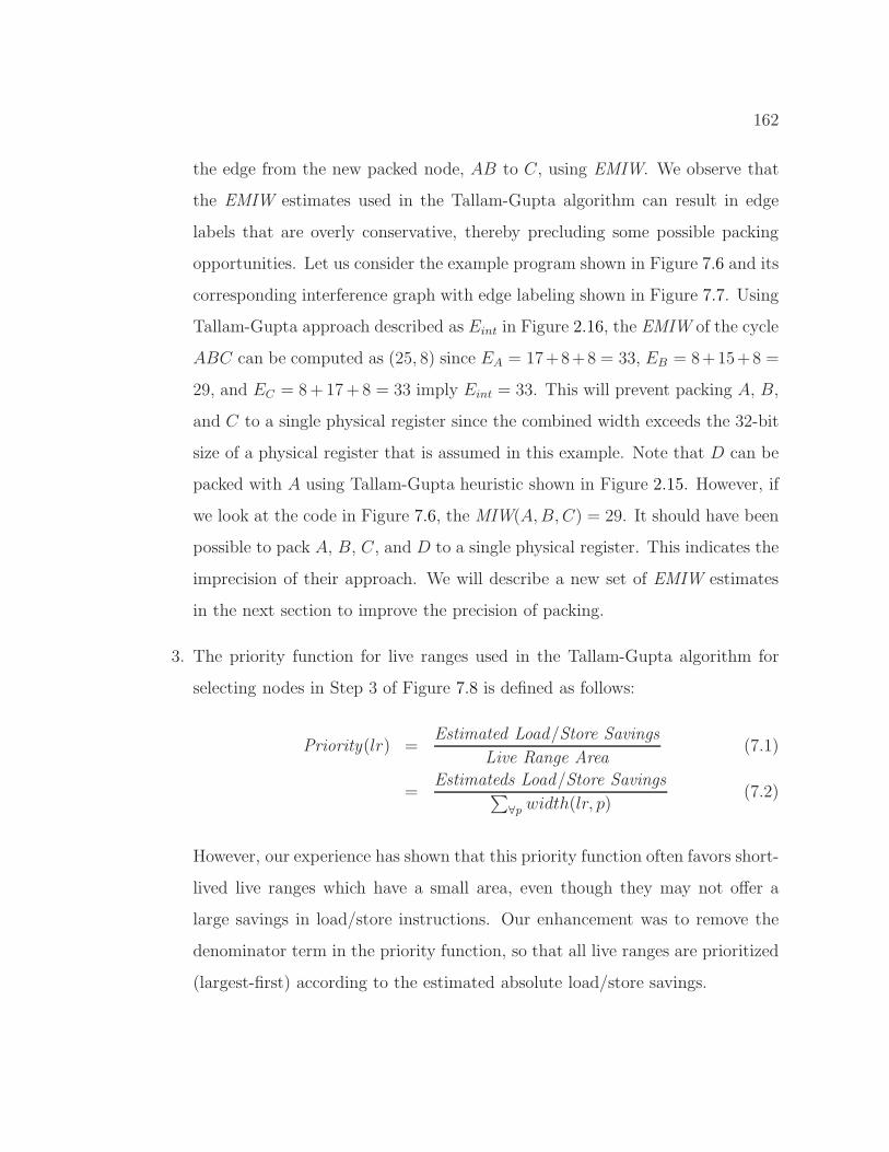
162
the edge from the new packed node, AB to C, using EMIW. We observe that
the EMIW estimates used in the Tallam-Gupta algorithm can result in edge
labels that are overly conservative, thereby precluding some possible packing
opportunities. Let us consider the example program shown in Figure 7.6 and its
corresponding interference graph with edge labeling shown in Figure 7.7. Using
Tallam-Gupta approach described as Eint in Figure 2.16, the EMIW of the cycle
ABC can be computed as (25, 8) since EA = 17+8+8 = 33, EB = 8+15+8 =
29, and EC = 8 +17 +8 = 33 imply Eint = 33. This will prevent packing A, B,
and C to a single physical register since the combined width exceeds the 32-bit
size of a physical register that is assumed in this example. Note that D can be
packed with A using Tallam-Gupta heuristic shown in Figure 2.15. However, if
we look at the code in Figure 7.6, the MIW(A, B, C) = 29. It should have been
possible to pack A, B, C, and D to a single physical register. This indicates the
imprecision of their approach. We will describe a new set of EMIW estimates
in the next section to improve the precision of packing.
3. The priority function for live ranges used in the Tallam-Gupta algorithm for
selecting nodes in Step 3 of Figure 7.8 is defined as follows:
Priority(lr) =Estimated Load/Store Savings
Live Range Area(7.1)
=Estimateds Load/Store Savings
∑
∀p width(lr, p)(7.2)
However, our experience has shown that this priority function often favors short-
lived live ranges which have a small area, even though they may not offer a
large savings in load/store instructions. Our enhancement was to remove the
denominator term in the priority function, so that all live ranges are prioritized
(largest-first) according to the estimated absolute load/store savings.
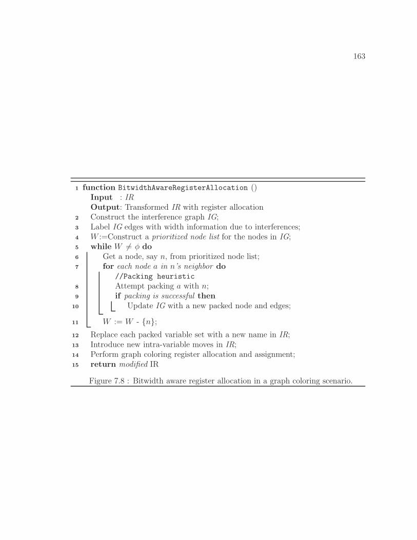
163
function BitwidthAwareRegisterAllocation ()1
Input : IROutput: Transformed IR with register allocationConstruct the interference graph IG;2
Label IG edges with width information due to interferences;3
W :=Construct a prioritized node list for the nodes in IG;4
while W 6= φ do5
Get a node, say n, from prioritized node list;6
for each node a in n’s neighbor do7
//Packing heuristic
Attempt packing a with n;8
if packing is successful then9
Update IG with a new packed node and edges;10
W := W - {n};11
Replace each packed variable set with a new name in IR;12
Introduce new intra-variable moves in IR;13
Perform graph coloring register allocation and assignment;14
return modified IR15
Figure 7.8 : Bitwidth aware register allocation in a graph coloring scenario.
164
7.4.1 Improved EMIW estimates
As mentioned in (2) above, the update of edge labels after variable packing can be
overly conservative in the Tallam-Gupta algorithm. Tallam-Gupta uses edge labels
in the interference graph to compute EMIW estimates to approximate the MIW
information. Our observation (motivated by the example shown in Figure 7.7) is that
the nodes in the interference graph can also be annotated with their maximum width
information that can be used in conjunction with edge labeling to obtain more precise
EMIW estimates. For the example program shown in Figure 7.7, the MIW of variables
A and C is 15+8 = 23. To this, if we add 8, which is the maximum width of B across
all program points, we will get EMIW(A, B, C) = 21+8 = 29 = MIW(A, B, C), which
is precise than Tallam-Gupta’s EMIW(A, B, C) = 33.
Let NODEMAX denotes the maximum width of a variable across all program
points. Using NODEMAX for every variable in the interference graph and Tallam-
Gupta’s edge labeling, we present a set of new E1, E2, E3, E4, E5 and E6 estimates
for EMIW as shown in Table 7.3. These EMIW estimates are used in conjunction
with the equations provided in Figure 2.16. The safety of the new precise estimates
trivially follow from the intermediate value theorem of Tallam-Gupta and is described
in [11].
7.5 Summary
In this chapter, we studied the problem of enhancing bitwidth-aware register alloca-
tion. Our limit study showed significant opportunities for improvement, compared
to the algorithm pioneered by Tallam and Gupta. The enhanced bitwidth analysis
that performs more detailed scalar analysis and array analysis results in improved
bitwidth information than in Tallam and Gupta. The enhanced packing algorithm
that performs less conservative (more aggressive) coalescing than in [116]. Also,
the proposed improved EMIW estimates result in improving the precision of packing
algorithm. Section 8.3 reports experimental evaluation of our proposed enhancements.
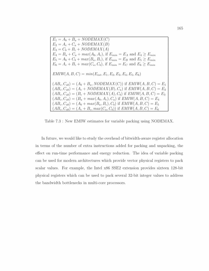
165
E1 = Ab + Ba + NODEMAX (C)E2 = Ac + Ca + NODEMAX (B)E3 = Cb + Bc + NODEMAX (A)E4 = Ba + Ca + max(Ab, Ac), if Emin = EA and E4 ≥ Emin
E5 = Ab + Cb + max(Ba, Bc), if Emin = EB and E5 ≥ Emin
E6 = Ac + Bc + max(Ca, Cb), if Emin = EC and E6 ≥ Emin
EMIW(A, B, C) = min(Eint, E1, E2, E3, E4, E5, E6)
(ABc, Cab) = (Ab + Ba,NODEMAX (C)) if EMIW(A, B, C) = E1
(ABc, Cab) = (Ac + NODEMAX (B), Ca) if EMIW(A, B, C) = E2
(ABc, Cab) = (Bc + NODEMAX (A), Cb) if EMIW(A, B, C) = E3
(ABc, Cab) = (Ba + max (Ab, Ac), Ca) if EMIW(A, B, C) = E4
(ABc, Cab) = (Ab + max(Ba, Bc), Cb) if EMIW(A, B, C) = E5
(ABc, Cab) = (Ac + Bc,max(Ca, Cb)) if EMIW(A, B, C) = E6
Table 7.3 : New EMIW estimates for variable packing using NODEMAX.
In future, we would like to study the overhead of bitwidth-aware register allocation
in terms of the number of extra instructions added for packing and unpacking, the
effect on run-time performance and energy reduction. The idea of variable packing
can be used for modern architectures which provide vector physical registers to pack
scalar values. For example, the Intel x86 SSE2 extension provides sixteen 128-bit
physical registers which can be used to pack several 32-bit integer values to address
the bandwidth bottlenecks in multi-core processors.
166
Chapter 8
Performance Results
In this chapter, we report on our experimental evaluation for the Side-effect Analysis
(described in Chapter 4), Scalar replacement for Load Elimination (described in
Chapter 5), Space-efficient Register Allocation (described in Chapter 6) and Bitwidth-
aware Register Allocation (described in Chapter 7). We use two compiler infras-
tructures to demonstrate the effectiveness of our techniques, Jikes RVM [66] and
GCC [56]. Scalar replacement techniques presented in this thesis were evaluated
in a Jikes RVM dynamic compilation environment for HJ programs. The register
allocation algorithms were evaluated both in Jikes RVM and GCC. Finally, the
enhancements to Bitwidth-aware register allocation were evaluated in GCC alone
since the standard set of benchmarks exposing bitwidth characteristics were written
mostly in C programming language.
8.1 Side-Effect Analysis and Load Elimination
We present an experimental evaluation of the scalar replacement for load elimination
algorithm introduced in Chapter 4 and Chapter 5 for a set of programs written in the
subset of HJ consisting of the async, finish and isolated parallel constructs.
8.1.1 Experimental setup
The performance results were obtained using Jikes RVM 3.0.0 [66] on a 16-core
system that has four 2.40GHz quad-core Intel Xeon processors running Red-Hat Linux
(RHEL 5). The system has 30GB of memory.
For our experimental evaluation, we use the production configuration of Jikes RVM
167
with the following options:-X:aos:initial compiler=opt -X:irc:O0. By default,
Jikes RVM does not enable SSA based HIR optimizations like scalar replacement for
load elimination transformation at optimization level O0. We modified Jikes RVM
to enable the SSA and load elimination phases at O0. However, since the focus of
our transformation is on optimizing application classes, the boot image was built
with scalar replacement for load elimination turned off and the same boot image was
used for all execution runs reported. The set of optimizations performed at O0 are:
copy propagation, constant propagation, common subexpression elimination, inline
allocation of scalar, inlining of statically resolved methods and linear scan register
allocation. The ParallelSideEffectAnalysis procedure presented in Figure 4.7 was
implemented as an HIR optimization pass in the OptimizationPlanner, and the new
scalar replacement for load elimination algorithm from Figure 5.3 was implemented
as an extension to the existing load elimination algorithm in Jikes RVM based on the
FKS algorithm [52].
All results were obtained using the -Xmx2000M JVM option to limit the heap size
to 2GB, thereby ensuring that the memory requirement for our experiments was well
below the available memory on the 16-core Intel Xeon SMP. The PLOS FRAC variable
in Plan.java was set to 0.4f for all runs, to ensure that the Large Object Size (LOS)
was large enough to accommodate all benchmarks. The main program was extended
with a five-iteration loop within the same Java process for all JVM runs, and the
best of the five times was reported in each case. This approach was chosen to reduce
the impact of dynamic compilation time and other virtual machine services in the
performance comparisons.
For our experiments, we used the five largest HJ programs that we could find
— three Section 3 Java Grande Forum (JGF) benchmarks (Moldyn, RayTracer,
Montecarlo) and two NAS Parallel (NPB) benchmarks (CG and MG). All JGF
benchmarks were run with the largest data size available. Sizes “A” and “W” were
used for CG and MG respectively, to ensure completion in a reasonable amount of
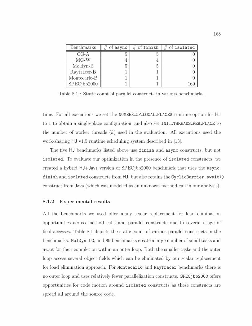
168
Benchmarks # of async # of finish # of isolated
CG-A 5 5 0MG-W 4 4 0
Moldyn-B 5 5 0Raytracer-B 1 1 0Montecarlo-B 1 1 0SPECjbb2000 1 1 169
Table 8.1 : Static count of parallel constructs in various benchmarks.
time. For all executions we set the NUMBER OF LOCAL PLACES runtime option for HJ
to 1 to obtain a single-place configuration, and also set INIT THREADS PER PLACE to
the number of worker threads (k) used in the evaluation. All executions used the
work-sharing HJ v1.5 runtime scheduling system described in [13].
The five HJ benchmarks listed above use finish and async constructs, but not
isolated. To evaluate our optimization in the presence of isolated constructs, we
created a hybrid HJ+Java version of SPECjbb2000 benchmark that uses the async,
finish and isolated constructs from HJ, but also retains the CyclicBarrier.await()
construct from Java (which was modeled as an unknown method call in our analysis).
8.1.2 Experimental results
All the benchmarks we used offer many scalar replacement for load elimination
opportunities across method calls and parallel constructs due to several usage of
field accesses. Table 8.1 depicts the static count of various parallel constructs in the
benchmarks. MolDyn, CG, and MG benchmarks create a large number of small tasks and
await for their completion within an outer loop. Both the smaller tasks and the outer
loop access several object fields which can be eliminated by our scalar replacement
for load elimination approach. For Montecarlo and RayTracer benchmarks there is
no outer loop and uses relatively fewer parallelization constructs. SPECjbb2000 offers
opportunities for code motion around isolated constructs as these constructs are
spread all around the source code.
169
We perform two additional compiler transformations that create more opportuni-
ties for scalar replacement and improved register allocation:
1. Loop-invariant getfield code motion pre-pass: In general, a loop-invariant getfield
operation cannot be moved out of a loop since it may throw a NullPointerException.
To address this case, we perform the standard transformation of replacing a
while loop by a zero-trip test and a repeat-until loop so as to enable loop-
invariant code motion of getfield operations while still preserving exception
semantics. This transformation is performed as a pre-pass to scalar replacement
for load elimination. We use the side-effect analysis described in Chapter 4 for
method calls inside the loop to determine if a getfield operation is loop-
invariant.
2. Live-range splitting post-pass: a potential negative impact of scalar replacement
is that increasing the size of live-ranges can lead to increased register pressure.
This in turn may cause a performance degradation if the register allocator
does not perform live-range splitting. Since the Linear Scan register allocator
in Jikes RVM currently does not split live-ranges, we introduce a live-range
splitting pass after load elimination that only splits live-ranges of the scalar
temporaries introduced by our optimizations. The live-ranges of these scalars
are split around all call instructions and loop entry-exit regions. This creates
smaller scalar live-ranges for which spilling and register assignment decisions
can be made separately. However, in some cases, this benefit can be undone
by the register allocator if it decides to coalesce the live ranges back before
allocation.
Experimental results are reported for the following cases:
1. 1-thread NOLOADELIM – Baseline measurement with no load elimination and
a single worker thread;
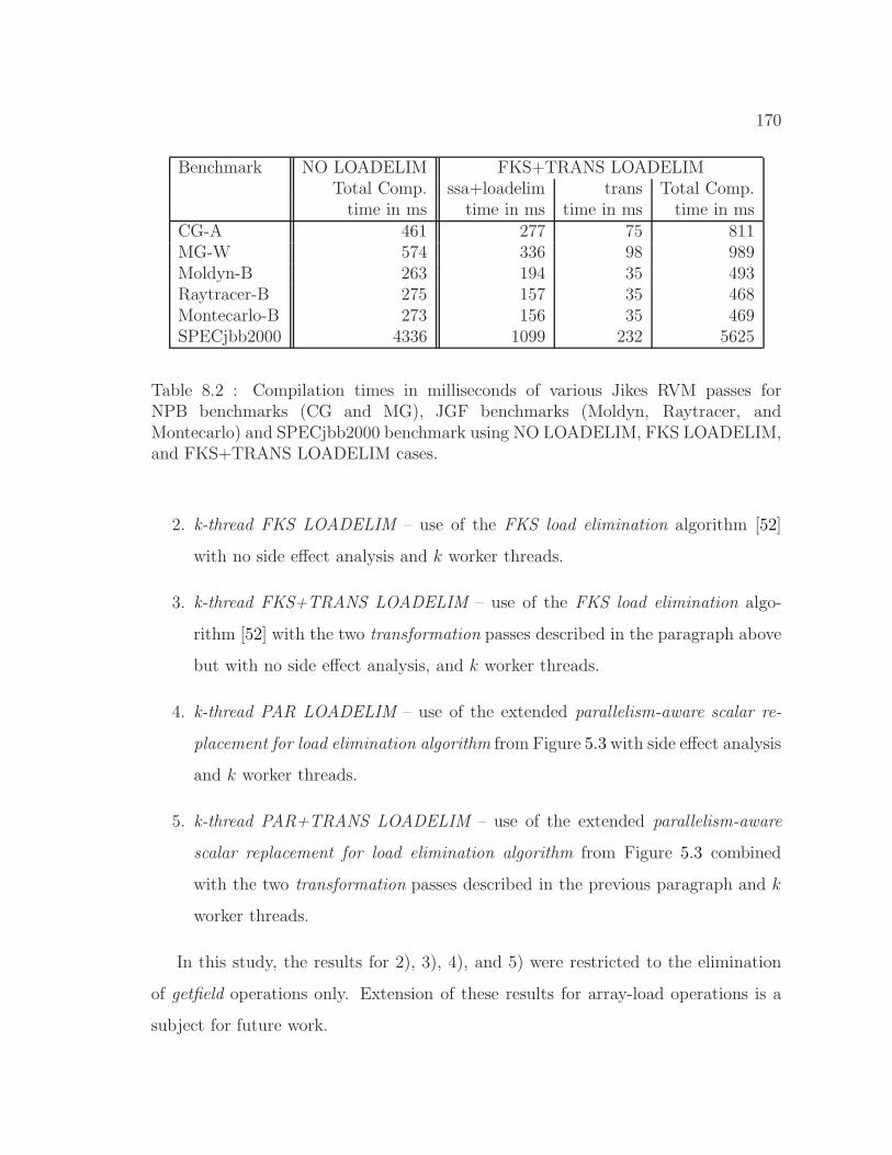
170
Benchmark NO LOADELIM FKS+TRANS LOADELIMTotal Comp. ssa+loadelim trans Total Comp.
time in ms time in ms time in ms time in msCG-A 461 277 75 811MG-W 574 336 98 989Moldyn-B 263 194 35 493Raytracer-B 275 157 35 468Montecarlo-B 273 156 35 469SPECjbb2000 4336 1099 232 5625
Table 8.2 : Compilation times in milliseconds of various Jikes RVM passes forNPB benchmarks (CG and MG), JGF benchmarks (Moldyn, Raytracer, andMontecarlo) and SPECjbb2000 benchmark using NO LOADELIM, FKS LOADELIM,and FKS+TRANS LOADELIM cases.
2. k-thread FKS LOADELIM – use of the FKS load elimination algorithm [52]
with no side effect analysis and k worker threads.
3. k-thread FKS+TRANS LOADELIM – use of the FKS load elimination algo-
rithm [52] with the two transformation passes described in the paragraph above
but with no side effect analysis, and k worker threads.
4. k-thread PAR LOADELIM – use of the extended parallelism-aware scalar re-
placement for load elimination algorithm from Figure 5.3 with side effect analysis
and k worker threads.
5. k-thread PAR+TRANS LOADELIM – use of the extended parallelism-aware
scalar replacement for load elimination algorithm from Figure 5.3 combined
with the two transformation passes described in the previous paragraph and k
worker threads.
In this study, the results for 2), 3), 4), and 5) were restricted to the elimination
of getfield operations only. Extension of these results for array-load operations is a
subject for future work.
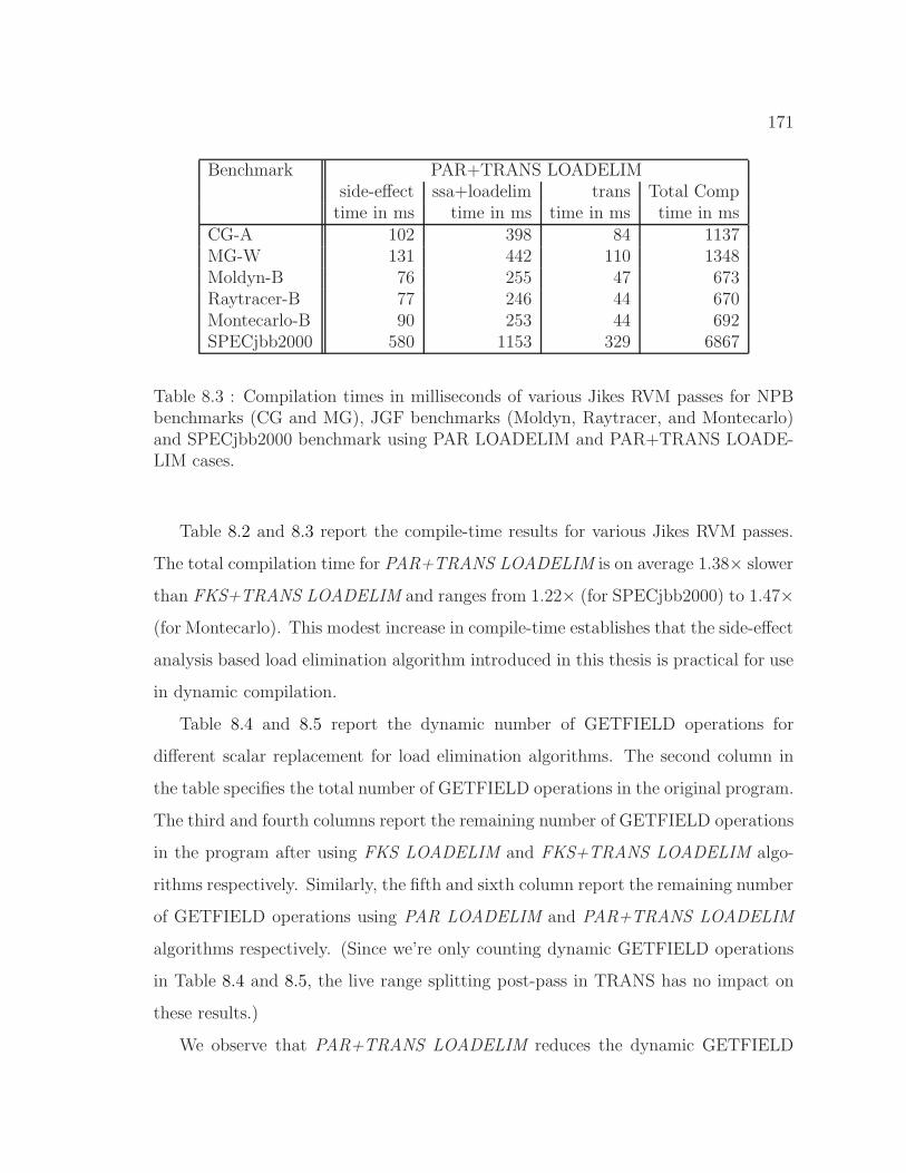
171
Benchmark PAR+TRANS LOADELIMside-effect ssa+loadelim trans Total Comp
time in ms time in ms time in ms time in msCG-A 102 398 84 1137MG-W 131 442 110 1348Moldyn-B 76 255 47 673Raytracer-B 77 246 44 670Montecarlo-B 90 253 44 692SPECjbb2000 580 1153 329 6867
Table 8.3 : Compilation times in milliseconds of various Jikes RVM passes for NPBbenchmarks (CG and MG), JGF benchmarks (Moldyn, Raytracer, and Montecarlo)and SPECjbb2000 benchmark using PAR LOADELIM and PAR+TRANS LOADE-LIM cases.
Table 8.2 and 8.3 report the compile-time results for various Jikes RVM passes.
The total compilation time for PAR+TRANS LOADELIM is on average 1.38× slower
than FKS+TRANS LOADELIM and ranges from 1.22× (for SPECjbb2000) to 1.47×(for Montecarlo). This modest increase in compile-time establishes that the side-effect
analysis based load elimination algorithm introduced in this thesis is practical for use
in dynamic compilation.
Table 8.4 and 8.5 report the dynamic number of GETFIELD operations for
different scalar replacement for load elimination algorithms. The second column in
the table specifies the total number of GETFIELD operations in the original program.
The third and fourth columns report the remaining number of GETFIELD operations
in the program after using FKS LOADELIM and FKS+TRANS LOADELIM algo-
rithms respectively. Similarly, the fifth and sixth column report the remaining number
of GETFIELD operations using PAR LOADELIM and PAR+TRANS LOADELIM
algorithms respectively. (Since we’re only counting dynamic GETFIELD operations
in Table 8.4 and 8.5, the live range splitting post-pass in TRANS has no impact on
these results.)
We observe that PAR+TRANS LOADELIM reduces the dynamic GETFIELD
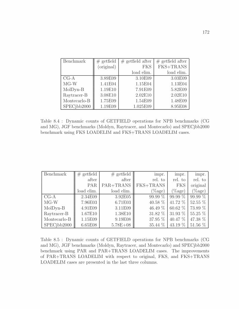
172
Benchmark # getfield # getfield after # getfield after(original) FKS FKS+TRANS
load elim. load elim.CG-A 3.89E09 3.10E09 3.03E09MG-W 1.41E04 1.15E04 1.13E04MolDyn-B 1.19E10 7.91E09 5.82E09Raytracer-B 3.08E10 2.02E10 2.02E10Montecarlo-B 1.75E09 1.54E09 1.48E09SPECjbb2000 1.19E09 1.025E09 8.95E08
Table 8.4 : Dynamic counts of GETFIELD operations for NPB benchmarks (CGand MG), JGF benchmarks (Moldyn, Raytracer, and Montecarlo) and SPECjbb2000benchmark using FKS LOADELIM and FKS+TRANS LOADELIM cases.
Benchmark # getfield # getfield impr. impr. impr.after after rel. to rel. to rel. toPAR PAR+TRANS FKS+TRANS FKS original
load elim. load elim. (%age) (%age) (%age)CG-A 2.34E09 3.92E05 99.99 % 99.99 % 99.99 %MG-W 7.96E03 6.71E03 40.58 % 41.72 % 52.55 %MolDyn-B 4.91E09 3.11E09 46.49 % 60.62 % 73.89 %Raytracer-B 1.67E10 1.38E10 31.82 % 31.93 % 55.25 %Montecarlo-B 1.15E09 9.19E08 37.95 % 40.47 % 47.38 %SPECjbb2000 6.65E08 5.78E+08 35.44 % 43.19 % 51.56 %
Table 8.5 : Dynamic counts of GETFIELD operations for NPB benchmarks (CGand MG), JGF benchmarks (Moldyn, Raytracer, and Montecarlo) and SPECjbb2000benchmark using PAR and PAR+TRANS LOADELIM cases. The improvementsof PAR+TRANS LOADELIM with respect to original, FKS, and FKS+TRANSLOADELIM cases are presented in the last three columns.
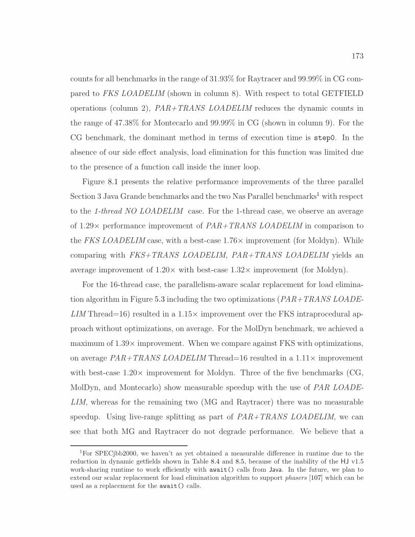
173
counts for all benchmarks in the range of 31.93% for Raytracer and 99.99% in CG com-
pared to FKS LOADELIM (shown in column 8). With respect to total GETFIELD
operations (column 2), PAR+TRANS LOADELIM reduces the dynamic counts in
the range of 47.38% for Montecarlo and 99.99% in CG (shown in column 9). For the
CG benchmark, the dominant method in terms of execution time is step0. In the
absence of our side effect analysis, load elimination for this function was limited due
to the presence of a function call inside the inner loop.
Figure 8.1 presents the relative performance improvements of the three parallel
Section 3 Java Grande benchmarks and the two Nas Parallel benchmarks1 with respect
to the 1-thread NO LOADELIM case. For the 1-thread case, we observe an average
of 1.29× performance improvement of PAR+TRANS LOADELIM in comparison to
the FKS LOADELIM case, with a best-case 1.76× improvement (for Moldyn). While
comparing with FKS+TRANS LOADELIM, PAR+TRANS LOADELIM yields an
average improvement of 1.20× with best-case 1.32× improvement (for Moldyn).
For the 16-thread case, the parallelism-aware scalar replacement for load elimina-
tion algorithm in Figure 5.3 including the two optimizations (PAR+TRANS LOADE-
LIM Thread=16) resulted in a 1.15× improvement over the FKS intraprocedural ap-
proach without optimizations, on average. For the MolDyn benchmark, we achieved a
maximum of 1.39× improvement. When we compare against FKS with optimizations,
on average PAR+TRANS LOADELIM Thread=16 resulted in a 1.11× improvement
with best-case 1.20× improvement for Moldyn. Three of the five benchmarks (CG,
MolDyn, and Montecarlo) show measurable speedup with the use of PAR LOADE-
LIM, whereas for the remaining two (MG and Raytracer) there was no measurable
speedup. Using live-range splitting as part of PAR+TRANS LOADELIM, we can
see that both MG and Raytracer do not degrade performance. We believe that a
1For SPECjbb2000, we haven’t as yet obtained a measurable difference in runtime due to thereduction in dynamic getfields shown in Table 8.4 and 8.5, because of the inability of the HJ v1.5work-sharing runtime to work efficiently with await() calls from Java. In the future, we plan toextend our scalar replacement for load elimination algorithm to support phasers [107] which can beused as a replacement for the await() calls.
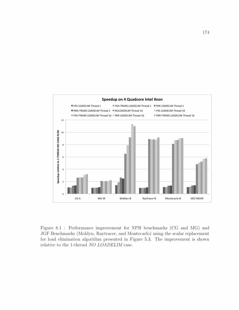
174
!"
#"
$"
%"
&"
'!"
'#"
()*+" ,)*-" ,./012*3" 451675897*3" ,.2:9857/.*3" );<",;+="
!"##$%"&'#()*+#&,-&./012345&67&8745&389:&
!"##$%"&-;&<&=%)$>-'#&9;,#(&?#-;&
>?@"A<+0;AB,"6C795D"'" >?@E64+=@"A<+0;AB,"6C795D"'" F+4"A<+0;AB,"6C795D"'"
F+4E64+=@"A<+0;AB,"6C795D"'" =<A<+0;AB,"6C795D"'%" >?@"A<+0;AB,"6C795D"'%"
>?@E64+=@"A<+0;AB,"6C795D"'%" F+4"A<+0;AB,"6C795D"'%" F+4E64+=@"A<+0;AB,"6C795D"'%"
Figure 8.1 : Performance improvement for NPB benchmarks (CG and MG) andJGF Benchmarks (Moldyn, Raytracer, and Montecarlo) using the scalar replacementfor load elimination algorithm presented in Figure 5.3. The improvement is shownrelative to the 1-thread NO LOADELIM case.
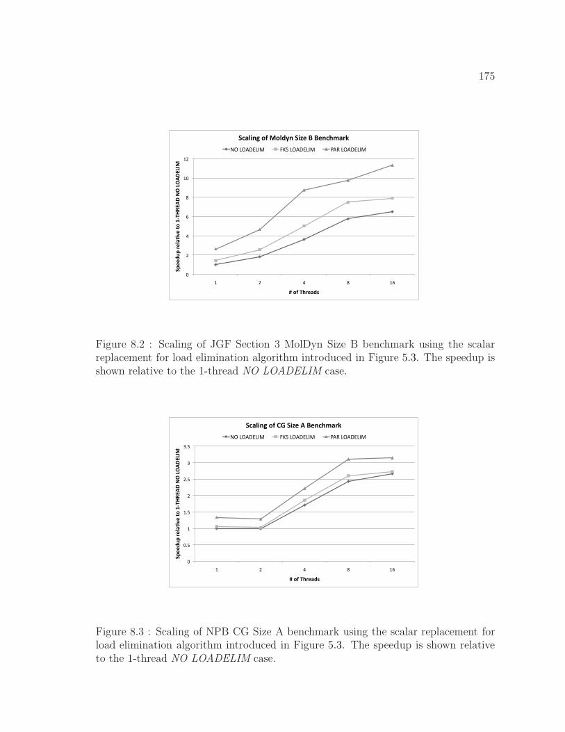
175
!"
#"
$"
%"
&"
'!"
'#"
'" #" $" &" '%"
!"##$%"&'#()*+#&,-&./012345&67&8745389:&
;&-<&0='#)$>&
!?)(@AB&-<&:-($CA&!@D#&E&E#A?=F)'G&
()"*)+,-*./" 012"*)+,-*./" 3+4"*)+,-*./"
Figure 8.2 : Scaling of JGF Section 3 MolDyn Size B benchmark using the scalarreplacement for load elimination algorithm introduced in Figure 5.3. The speedup isshown relative to the 1-thread NO LOADELIM case.
!"
!#$"
%"
%#$"
&"
&#$"
'"
'#$"
%" &" (" )" %*"
!"##$%"&'#()*+#&,-&./012345&67&8745389:&
;&-<&0='#)$>&
!?)(@AB&-<&CD&!@E#&4&F#A?=G)'H&
+,"-,./0-12" 345"-,./0-12" 6.7"-,./0-12"
Figure 8.3 : Scaling of NPB CG Size A benchmark using the scalar replacement forload elimination algorithm introduced in Figure 5.3. The speedup is shown relativeto the 1-thread NO LOADELIM case.
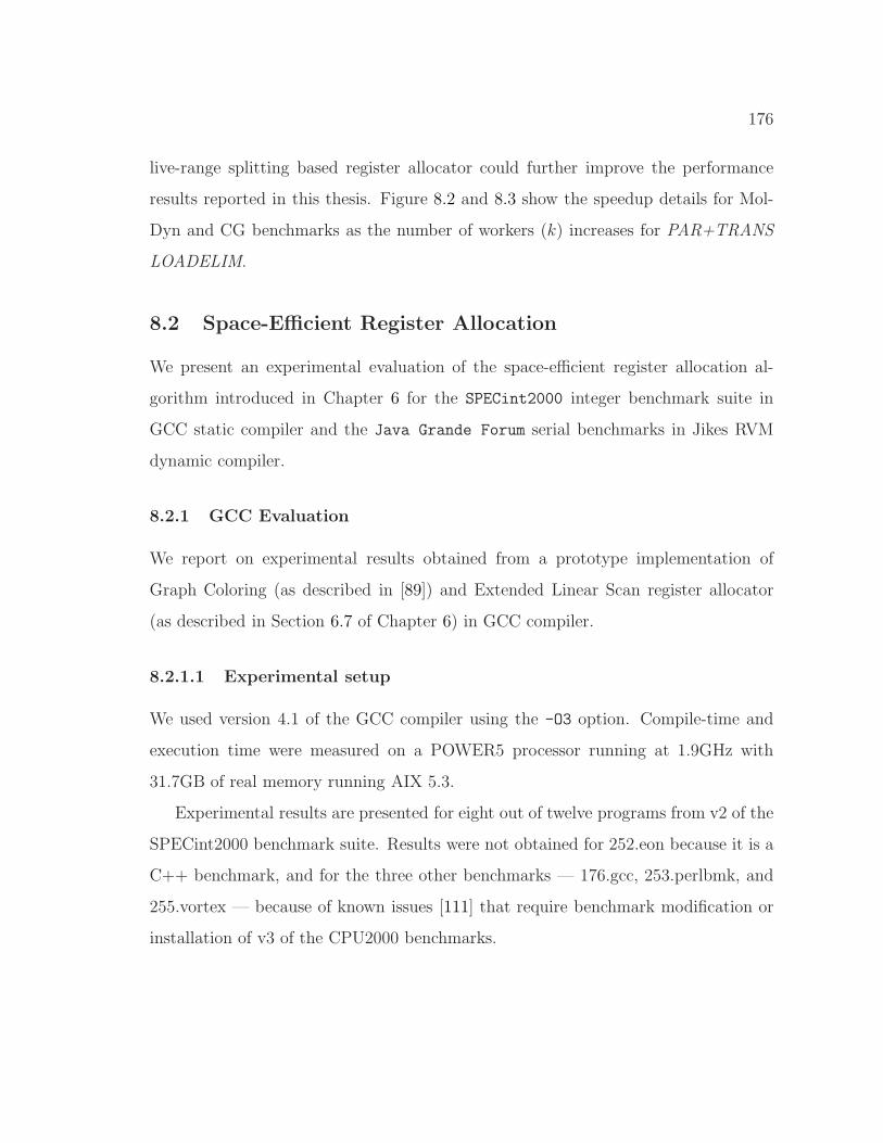
176
live-range splitting based register allocator could further improve the performance
results reported in this thesis. Figure 8.2 and 8.3 show the speedup details for Mol-
Dyn and CG benchmarks as the number of workers (k) increases for PAR+TRANS
LOADELIM.
8.2 Space-Efficient Register Allocation
We present an experimental evaluation of the space-efficient register allocation al-
gorithm introduced in Chapter 6 for the SPECint2000 integer benchmark suite in
GCC static compiler and the Java Grande Forum serial benchmarks in Jikes RVM
dynamic compiler.
8.2.1 GCC Evaluation
We report on experimental results obtained from a prototype implementation of
Graph Coloring (as described in [89]) and Extended Linear Scan register allocator
(as described in Section 6.7 of Chapter 6) in GCC compiler.
8.2.1.1 Experimental setup
We used version 4.1 of the GCC compiler using the -O3 option. Compile-time and
execution time were measured on a POWER5 processor running at 1.9GHz with
31.7GB of real memory running AIX 5.3.
Experimental results are presented for eight out of twelve programs from v2 of the
SPECint2000 benchmark suite. Results were not obtained for 252.eon because it is a
C++ benchmark, and for the three other benchmarks — 176.gcc, 253.perlbmk, and
255.vortex — because of known issues [111] that require benchmark modification or
installation of v3 of the CPU2000 benchmarks.
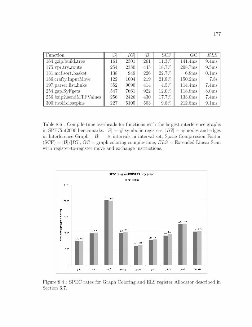
177
Function |S| |IG| |B| SCF GC ELS164.gzip.build tree 161 2301 261 11.3% 141.4ms 9.4ms175.vpr.try route 254 2380 445 18.7% 208.7ms 9.5ms181.mcf.sort basket 138 949 226 22.7% 6.8ms 0.1ms186.crafty.InputMove 122 1004 219 21.8% 150.2ms 7.8s197.parser.list links 352 9090 414 4.5% 114.4ms 7.4ms254.gap.SyFgets 547 7661 922 12.0% 118.8ms 8.0ms256.bzip2.sendMTFValues 256 2426 430 17.7% 133.0ms 7.4ms300.twolf.closepins 227 5105 503 9.8% 212.8ms 9.1ms
Table 8.6 : Compile-time overheads for functions with the largest interference graphsin SPECint2000 benchmarks. |S| = # symbolic registers, |IG| = # nodes and edgesin Interference Graph , |B| = # intervals in interval set, Space Compression Factor(SCF) = |B|/|IG|, GC = graph coloring compile-time, ELS = Extended Linear Scanwith register-to-register move and exchange instructions.
Figure 8.4 : SPEC rates for Graph Coloring and ELS register Allocator described inSection 6.7.
178
8.2.1.2 Experimental results
Table 8.6 summarizes compile-time overheads of the Graph Coloring and ELS regis-
ter allocation algorithm. The measurements were obtained for functions with the
largest interference graphs in the eight SPECint2000 benchmarks, using the -O3
-finline-limit=3000 -ftime-report options in gcc. It is interesting to note that
the Interference Graph size, |IG|, typically grows as O(|S|1.5), whereas the number
of intervals, |B| is always ≤ 2|S|. This is one of the important reasons behind the
compile-time efficiency of the Linear Scan and ELS register allocation algorithms.
While it is theoretically possible for the number of intervals for a symbolic register
to be as high as half the total number of instructions in the program (e.g., if every
alternate instruction is a “hole” – which could lead to a non-linear complexity for
the ELS register allocator), we see that in practice the average number of intervals
per symbolic register is bounded by a small constant (≈ 2). We see that the Space
Compression Factor (SCF) = |B|/|IG| varies from 4.5% to 22.7%, indicating the
extent to which we expect the interval set, B to be smaller than the interference
graph, IG. Finally, the last two columns contain the compile-time spent in global
register allocation for these two algorithms. For improved measurement accuracy,
the register allocation phase was repeated 100 times, and the timing (in ms) reported
in Table 8.6 is the average over the 100 runs. While compile-time measurements
depend significantly on the engineering of the algorithm implementations, the early
indications are there is a marked reduction in compile-time when moving from GC
to ELS register allocation for all benchmarks. The compile-time speedups for ELS
register allocator relative to GC varied from 15× to 68×, with an overall speedup of
18.5× when adding all the compile-times.
Figure 8.4 shows the SPEC rates obtained for the Graph Coloring and ELS register
allocation algorithms, using the -O3 option in GCC. Recall that a larger SPEC rate
indicates better performance. In summary, the runtime performance improved by
up to 5.8% for the ELS register allocator relative to GC (for 197.parser), with an
179
average improvement of 2.3%. There was only one case in which a small performance
degradation was observed for the ELS register allocator, relative to GC – a slowdown
of 1.4% for 181.mcf. These results clearly show that the compile-time benefits for
Extended Linear Scan can be obtained without sacrificing runtime performance —
in fact, ELS register allocator delivers a net improvement in runtime performance
relative to GC. Further, the results indicate that the extra register-to-register moves
did not contribute a significant performance degradation.
8.2.2 Jikes RVM evaluation
We present an experimental evaluation of the Bipartite Liveness Graph (BLG) based
constrained register allocation and assignment algorithms presented in Section 6.6 of
Chapter 6.
8.2.2.1 Experimental setup
The experimental setup uses Jikes RVM 3.0.0 [66] dynamic compiler on an Intel
Xeon 2.4GHz system with 30GB of memory and running Red-Hat Linux (RHEL 5).
We used the serial version of the Java Grande Form (JGF) benchmark suite [65] to
evaluate the performance of our register allocator.
The serial programs in the JGF benchmark suite comprises of seven Section 2
benchmarks (Crypt, Heapsort, Sparsematmult, Sor, Series, LUFact, and FFT)
and five larger Section 3 benchmarks (Raytracer, Moldyn, Montecarlo, Euler, and
Search). Of these, Jikes RVM was unable to execute the FFT benchmark due to VM
errors, so we present results for the remaining eleven. Further, the execution times
were obtained for the Section 2 benchmarks at optimization level O2 and for Section 3
benchmarks at optimization level O0. (Jikes RVM was unable to execute Section 3
benchmarks at a higher optimization level than O0 due to compilation errors.) The
boot image for Jikes RVM used a production configuration with a modification to
PLOS FRAC that was set to 0.4f to ensure that Jikes RVM had a Large Object Space
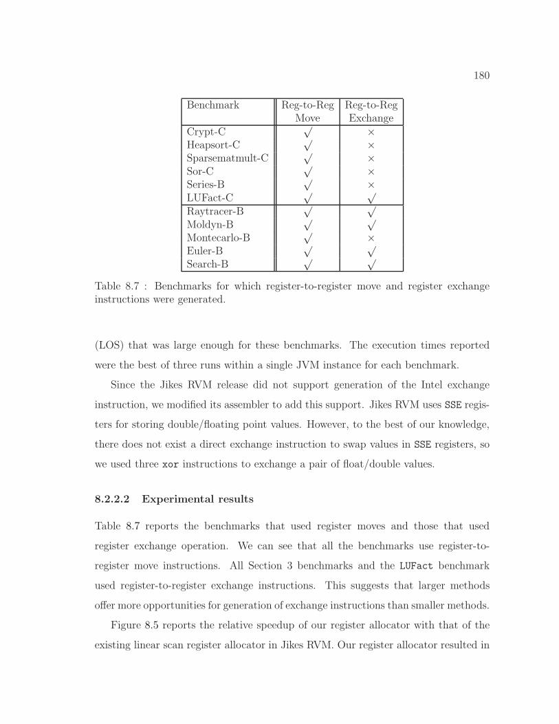
180
Benchmark Reg-to-Reg Reg-to-RegMove Exchange
Crypt-C√ ×
Heapsort-C√ ×
Sparsematmult-C√ ×
Sor-C√ ×
Series-B√ ×
LUFact-C√ √
Raytracer-B√ √
Moldyn-B√ √
Montecarlo-B√ ×
Euler-B√ √
Search-B√ √
Table 8.7 : Benchmarks for which register-to-register move and register exchangeinstructions were generated.
(LOS) that was large enough for these benchmarks. The execution times reported
were the best of three runs within a single JVM instance for each benchmark.
Since the Jikes RVM release did not support generation of the Intel exchange
instruction, we modified its assembler to add this support. Jikes RVM uses SSE regis-
ters for storing double/floating point values. However, to the best of our knowledge,
there does not exist a direct exchange instruction to swap values in SSE registers, so
we used three xor instructions to exchange a pair of float/double values.
8.2.2.2 Experimental results
Table 8.7 reports the benchmarks that used register moves and those that used
register exchange operation. We can see that all the benchmarks use register-to-
register move instructions. All Section 3 benchmarks and the LUFact benchmark
used register-to-register exchange instructions. This suggests that larger methods
offer more opportunities for generation of exchange instructions than smaller methods.
Figure 8.5 reports the relative speedup of our register allocator with that of the
existing linear scan register allocator in Jikes RVM. Our register allocator resulted in
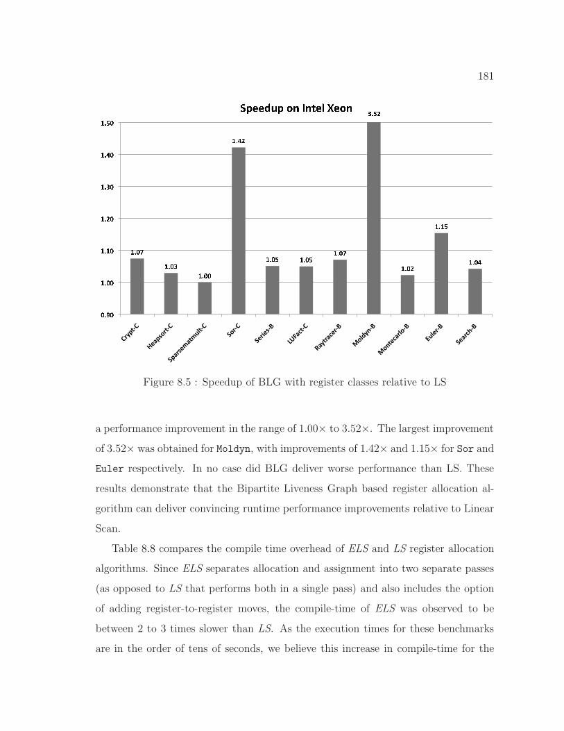
181
Figure 8.5 : Speedup of BLG with register classes relative to LS
a performance improvement in the range of 1.00× to 3.52×. The largest improvement
of 3.52× was obtained for Moldyn, with improvements of 1.42× and 1.15× for Sor and
Euler respectively. In no case did BLG deliver worse performance than LS. These
results demonstrate that the Bipartite Liveness Graph based register allocation al-
gorithm can deliver convincing runtime performance improvements relative to Linear
Scan.
Table 8.8 compares the compile time overhead of ELS and LS register allocation
algorithms. Since ELS separates allocation and assignment into two separate passes
(as opposed to LS that performs both in a single pass) and also includes the option
of adding register-to-register moves, the compile-time of ELS was observed to be
between 2 to 3 times slower than LS. As the execution times for these benchmarks
are in the order of tens of seconds, we believe this increase in compile-time for the
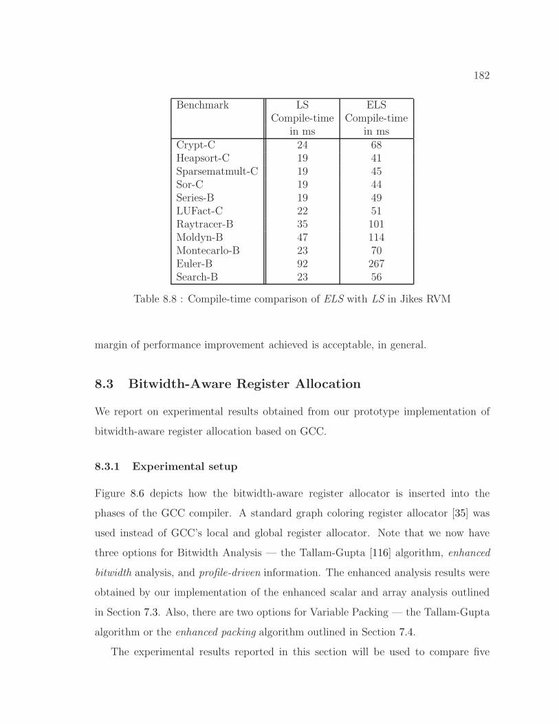
182
Benchmark LS ELSCompile-time Compile-time
in ms in msCrypt-C 24 68Heapsort-C 19 41Sparsematmult-C 19 45Sor-C 19 44Series-B 19 49LUFact-C 22 51Raytracer-B 35 101Moldyn-B 47 114Montecarlo-B 23 70Euler-B 92 267Search-B 23 56
Table 8.8 : Compile-time comparison of ELS with LS in Jikes RVM
margin of performance improvement achieved is acceptable, in general.
8.3 Bitwidth-Aware Register Allocation
We report on experimental results obtained from our prototype implementation of
bitwidth-aware register allocation based on GCC.
8.3.1 Experimental setup
Figure 8.6 depicts how the bitwidth-aware register allocator is inserted into the
phases of the GCC compiler. A standard graph coloring register allocator [35] was
used instead of GCC’s local and global register allocator. Note that we now have
three options for Bitwidth Analysis — the Tallam-Gupta [116] algorithm, enhanced
bitwidth analysis, and profile-driven information. The enhanced analysis results were
obtained by our implementation of the enhanced scalar and array analysis outlined
in Section 7.3. Also, there are two options for Variable Packing — the Tallam-Gupta
algorithm or the enhanced packing algorithm outlined in Section 7.4.
The experimental results reported in this section will be used to compare five
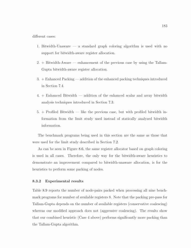
183
different cases:
1. Bitwidth-Unaware — a standard graph coloring algorithm is used with no
support for bitwidth-aware register allocation.
2. + Bitwidth-Aware — enhancement of the previous case by using the Tallam-
Gupta bitwidth-aware register allocation.
3. + Enhanced Packing — addition of the enhanced packing techniques introduced
in Section 7.4.
4. + Enhanced Bitwidth — addition of the enhanced scalar and array bitwidth
analysis techniques introduced in Section 7.3.
5. + Profiled Bitwidth — like the previous case, but with profiled bitwidth in-
formation from the limit study used instead of statically analyzed bitwidth
information.
The benchmark programs being used in this section are the same as those that
were used for the limit study described in Section 7.2.
As can be seen in Figure 8.6, the same register allocator based on graph coloring
is used in all cases. Therefore, the only way for the bitwidth-aware heuristics to
demonstrate an improvement compared to bitwidth-unaware allocation, is for the
heuristics to perform some packing of nodes.
8.3.2 Experimental results
Table 8.9 reports the number of node-pairs packed when processing all nine bench-
mark programs for number of available registers 8. Note that the packing pre-pass for
Tallam-Gupta depends on the number of available registers (conservative coalescing)
whereas our modified approach does not (aggressive coalescing). The results show
that our combined heuristic (Case 4 above) performs significantly more packing than
the Tallam-Gupta algorithm.
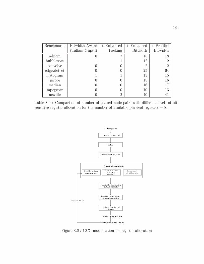
184
Benchmarks Bitwidth-Aware + Enhanced + Enhanced + Profiled(Tallam-Gupta) Packing Bitwidth Bitwidth
adpcm 0 7 15 18bubblesort 1 1 12 12convolve 0 0 2 2
edge detect 0 0 25 64histogram 1 1 15 15
jacobi 0 0 15 16median 0 0 16 17
mpegcorr 0 0 10 13newlife 0 2 40 41
Table 8.9 : Comparison of number of packed node-pairs with different levels of bit-sensitive register allocation for the number of available physical registers = 8.
bitwidth info
Bitwidth Analysis
Variable Coalescingwith or without improvements
Executable code
Register allocation via graph coloring
Other Backendphases
Program Execution
Compile time
analysisbitwidth
Profile−driven Enhancedbitwidth info
Backend phases
RTL
GCC Frontend
C Program
Profile Info
Figure 8.6 : GCC modification for register allocation
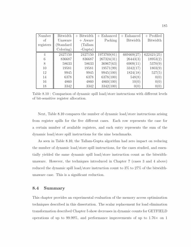
185
Number Bitwidth + Bitwidth + Enhanced + Enhanced + Profiledof Unaware + Aware Packing Bitwidth Bitwidth
registers (Standard (TallamColoring) -Gupta)
4 2427150 2427150 1973769(81) 669469(27) 622421(25)6 836687 836687 267324(31) 26443(3) 18953(2)8 58633 58633 36967(63) 6909(11) 5370(9)10 19581 19581 19571(99) 3342(17) 1803(9)12 9945 9945 9945(100) 1824(18) 527(5)14 6378 6378 6378(100) 548(8) 0(0)16 4860 4860 4860(100) 10(0) 0(0)18 3342 3342 3342(100) 0(0) 0(0)
Table 8.10 : Comparison of dynamic spill load/store instructions with different levelsof bit-sensitive register allocation.
Next, Table 8.10 compares the number of dynamic load/store instructions arising
from register spills for the five different cases. Each row represents the case for
a certain number of available registers, and each entry represents the sum of the
dynamic load/store spill instructions for the nine benchmarks.
As seen in Table 8.10, the Tallam-Gupta algorithm had zero impact on reducing
the number of dynamic load/store spill instructions, for the cases studied, and essen-
tially yielded the same dynamic spill load/store instruction count as the bitwidth-
unaware. However, the techniques introduced in Chapter 7 (cases 3 and 4 above)
reduced the dynamic spill load/store instruction count to 3% to 27% of the bitwidth-
unaware case. This is a significant reduction.
8.4 Summary
This chapter provides an experimental evaluation of the memory access optimization
techniques described in this dissertation. The scalar replacement for load elimination
transformation described Chapter 5 show decreases in dynamic counts for GETFIELD
operations of up to 99.99%, and performance improvements of up to 1.76× on 1
186
core, and 1.39× on 16 cores, when compared to the load elimination algorithm
available in Jikes RVM. A prototype implementation of our BLG register allocation
phase combined with the constrained assignment in Jikes RVM demonstrates runtime
performance improvements of up to 3.52× relative to the Linear Scan on an x86
processor. An evaluation of our Extended Linear Scan register allocator in GCC
show that the compile-time speedups for ELS relative to GC were significant, and
varied from 15× to 68×. In addition, the resulting execution time improved by up
to 5.8%, with an average improvement of 2.3% on a POWER5 processor. Finally,
the enhancements to bitwidth-aware register allocation described in Chapter 7 can
reduce the number of dynamic spill load/store instructions to between 3% and 27%.
The experimental evaluations combined with the foundations presented in this dis-
sertation, we strongly believe that the proposed high-level and low-level optimizations
are useful in addressing some of the new challenges emerging in efficient optimization
of parallel programs for multi-core architectures.
187
Chapter 9
Conclusions and Future Work
In this dissertation, we have presented a combination of high-level and low-level
compiler analyses and optimizations to address the Memory Wall problem in multi-
core architectures. The high level analyses include May-Happen-in-Parallel (MHP)
analysis and Side-Effect Analysis for any language that adopts the core concepts of
places, async, finish, and isolated from the HJ programming model. The low
level optimizations include Scalar replacement for Load Elimination and Register
Allocation.
We introduced a new algorithm for May-Happen-in-Parallel (MHP) analysis for
HJ programming model. The main contributions of this work compared to past MHP
analysis algorithms are as follows:
1. We introduced a more precise definition of the MHP relation than in past work
by adding condition vectors that identify execution instances for which the MHP
relation holds, instead of just returning a single true/false value for all pairs of
executing instances.
2. Compared to past work, the availability of basic concurrency control constructs
such as async and finish enabled the use of more efficient and precise analysis
algorithms based on simple path traversals in the Program Structure Tree, and
did not rely on interprocedural pointer alias analysis of thread objects as in
MHP analysis for the Java language.
3. We introduced place equivalence (PE) analysis to identify execution instances
that happen at the same place. The PE analysis helps us in leveraging the fact
188
that two statement instances which occur in atomic sections that execute at the
same X10 place must have MHP = false.
We introduced an interprocedural scalar replacement for load elimination algo-
rithm for dynamic optimization of parallel programs. The main contributions of our
work include: a) side-effect analysis of method calls, b) support for scalar replacement
for load elimination in the presence of three core parallel constructs – async, finish,
and isolated, c) an IC memory model that establishes the legality of our load
elimination transformation for parallel constructs, and d) performance results to
study the impact of scalar replacement on a set of standard HJ parallel programs.
Our performance results show decreases in dynamic counts for getfield operations of
up to 99.99%, and performance improvements of up to 1.76× on 1 core, and 1.39×on 16 cores, when comparing the algorithm in this paper with the load elimination
algorithm available in Jikes RVM. The algorithm has been implemented in Jikes RVM
for optimizing a subset of HJ parallel programs.
We addressed the problem of space-efficient register allocation. Most approaches
to register allocation involve the construction of an interference graph, which is
known from past work to be a major space and time bottleneck [42, 105]. A notable
exception is the Linear Scan algorithm which is favored by many dynamic and just-in-
time compilers because it avoids the overhead of constructing an interference graph.
In this thesis, we introduced a new approach to register allocation that improves
on the runtime performance delivered by Linear Scan, without exceeding its space
bound. To that end, we introduced a Bipartite Liveness Graph representation as
an alternative foundation to the interference graph. Allocation with the BLG is
formulated as an optimization problem and a greedy heuristic is presented to solve it.
We also formulated spill-free register assignment combined with move coalescing as
a combined optimization problem using the Coalesce Graph, which models both IR
move instructions and additional register-to-register moves/exchanges arising from
register assignment. We then extended the above register allocation and assignment
189
approaches to handle register classes. Our experimental results for 11 serial Java
Grande benchmarks compared our BLG based register allocation with that of the
existing Linear Scan (LS) register allocator in Jikes RVM. The results show that a
BLG based register allocation can achieve runtime benefits of up to 3.52× compared
to LS.
We studied the problem of enhancing bitwidth-aware register allocation. Our limit
study showed significant opportunities for improvement, compared to the algorithm
pioneered by Tallam-Gupta. We used our prototype implementation of bitwidth-
aware register allocation in gcc to compare the dynamic number of load/store instruc-
tions) resulting from a) bitwidth-unaware allocation, b) bitwidth-aware allocation, c)
enhanced bitwidth-aware allocation with improved bitwidth analysis and improved
packing, and d) ideal profile-driven bitwidth-aware allocation. Our results show that
our enhancements can reduce the dynamic number of spill load/store instructions to
3% to 27% of the number obtained from the Tallam-Gupta algorithm.
9.1 Future Work
The May-Happen-in-Parallel analysis presented in this dissertation can be enriched
using distance vectors and can be applied in an interprocedural context. The same can
also be improved to handle other synchronization constructs of HJ including phasers
and delayed async. Possible directions for future work for scalar replacement include
improving the precision of our analysis using MHP analysis. Also, our techniques can
be implemented for array accesses that go beyond simple field accesses. Directions for
future work in space-efficient register allocation include further study of the trade-off
between register-move instructions and spill load/store instructions, and support for
partial spill using live-range splitting. The bitwidth aware register allocation needs
to study the overhead of bit-aware register allocation (number of extra instructions
added), effect on run-time performance and energy reduction.
190
Bibliography
[1] N. Adiga et al. An overview of the BlueGene/L Supercomputer. In Supercom-
puting ’02: Proceedings of the 2002 ACM/IEEE conference on Supercomputing,
pages 1–22, Los Alamitos, CA, USA, 2002. IEEE Computer Society Press.
[2] S. Agarwal, R. Barik, V. Sarkar, and R. K. Shyamasundar. May-happen-in-
parallel analysis of X10 programs. In PPoPP ’07: Proceedings of the 12th ACM
SIGPLAN symposium on Principles and Practice of Parallel Programming,
pages 183–193, New York, NY, USA, 2007. ACM Press. ISBN 978-1-59593-
602-8. doi: http://doi.acm.org/10.1145/1229428.1229471.
[3] S. Agarwal, R. Barik, V. K. Nandivada, R. K. Shyamasundar, and P. Varma.
Static Detection of Place Locality and Elimination of Runtime Checks. The
Sixth ASIAN Symposium on Programming Languages and Systems, 2008.
[4] A. V. Aho, R. Sethi, and J. D. Ullman. Compilers: Principles, Techniques, and
Tools. Addison-Wesley, Reading, MA, 1986.
[5] F. E. Allen and J. Cocke. A catalogue of optimizing transformations. In Design
and Optimization of Compilers, pages 1–30. Prentice-Hall, 1972.
[6] B. Alpern, M. N. Wegman, and F. K. Zadeck. Detecting equality of variables
in programs. In POPL ’88: Proceedings of the 15th ACM SIGPLAN-SIGACT
symposium on Principles of Programming Languages, pages 1–11, New York,
NY, USA, 1988. ACM Press. ISBN 0-89791-252-7. doi: http://doi.acm.org/10.
1145/73560.73561.
191
[7] L. O. Andersen. Program analysis and specialization for the c programming
language. Technical report, 1994.
[8] A. W. Appel. Modern Compiler Implementation in Java. Cambridge University
Press, second edition, October 2002. ISBN 052182060X.
[9] J. P. Banning. An efficient way to find the side effects of procedure calls and
the aliases of variables. In POPL ’79: Proceedings of the 6th ACM SIGACT-
SIGPLAN symposium on Principles of Programming Languages, pages 29–41,
New York, NY, USA, 1979. ACM. doi: http://doi.acm.org/10.1145/567752.
567756.
[10] R. Barik. Efficient Computation of May-Happen-in-Parallel Information for
Concurrent Java Programs. In 18th International Workshop on Languages and
Compilers for Parallel Computing, October 2005.
[11] R. Barik and V. Sarkar. Enhanced Bitwidth-Aware Register Allocation. In
Proceedings of the 2006 International Conference on Compiler Construction
(CC 2006), March 2006.
[12] R. Barik and V. Sarkar. Interprocedural load elimination for dynamic optimiza-
tion of parallel programs. In International Conference on Parallel Architectures
and Compilation Techniques, (PACT’09), North Carolina, September 2009.
[13] R. Barik, V. Cave, C. Donawa, A. Kielstra, I. Peshansky, and V. Sarkar.
Experiences with an SMP Implementation for X10 based on the Java Concur-
rency Utilities (Extended Abstract). In Proceedings of the 2006 Workshop on
Programming Models for Ubiqui-tous Parallelism, co-located with PACT 2006,
September 2006, Seattle, Washington, 2006.
[14] L. A. Belady. A study of replacement algorithms for a virtual-storage computer.
IBM Syst. J., 5(2):78–101, 1966.
192
[15] D. Berlin, D. Edelsohn, and S. Pop. High-Level Loop Optimizations for GCC.
In The 2004 GCC Developers’ Summit, 2004.
[16] A. Berry, J. R. S. Blair, P. Heggernes, and B. W. Peyton. Maximum
Cardinality Search for Computing Minimal Triangulations of Graphs. Algorith-
mica, 39(4):287–298, 2004. ISSN 0178-4617. doi: http://dx.doi.org/10.1007/
s00453-004-1084-3.
[17] Bitwise. Bitwise benchmarks. http://www.cag.lcs.mit.edu/bitwise/bitwise benc
hmarks.htm.
[18] R. Blumofe, C. Joerg, B. Kuszmaul, C. Leiserson, K. Randall, and Y. Zhou.
Cilk: An Efficient Multithreaded Runtime System. In Proceedings of the
Fifth ACM SIGPLAN Symposium on Principles and Practice of Parallel
Programming (PPOPP), Santa Barbara California, July 19-21, pages 207–216,
1995.
[19] R. Bodik and R. Gupta. Array Data-Flow Analysis for Load-Store Optimiza-
tions in Superscalar Architectures. Lecture Notes in Computer Science, (1033):
1–15, August 1995. Proceedings of Eighth Annual Workshop on Languages and
Compilers for Parallel Computing, Columbus, Ohio.
[20] R. Bodık, R. Gupta, and M. L. Soffa. Load-reuse analysis: design and
evaluation. SIGPLAN Not., 34(5):64–76, 1999. ISSN 0362-1340. doi: http:
//doi.acm.org/10.1145/301631.301643.
[21] H.-J. Boehm and S. V. Adve. Foundations of the C++ concurrency memory
model. In PLDI ’08: Proceedings of the 2008 ACM SIGPLAN conference on
Programming Language Design and Implementation, pages 68–78, New York,
NY, USA, 2008. ACM. ISBN 978-1-59593-860-2. doi: http://doi.acm.org/10.
1145/1375581.1375591.
193
[22] F. Bouchez. A Study of Spilling and Coalescing in Register Allocation as Two
Separate Phases. PhD thesis, April 2009.
[23] F. Bouchez, A. Darte, and F. Rastello. On the Complexity of Register
Coalescing. In CGO ’07: Proceedings of the International Symposium on Code
Generation and Optimization, pages 102–114, Washington, DC, USA, 2007.
IEEE Computer Society. ISBN 0-7695-2764-7. doi: http://dx.doi.org/10.1109/
CGO.2007.26.
[24] P. Briggs. Register allocation via graph coloring. Technical Report TR92-183,
Rice University, Houston, Texas, 1998.
[25] P. Briggs, K. D. Cooper, K. Kennedy, and L. Torczon. Coloring Heuristics
for Register Allocation. Proceedings of the 1989 SIGPLAN Conference on
Programming Language Design and Implementation, 24(7):275–284, July 1989.
[26] P. Briggs, K. D. Cooper, and L. Torczon. Coloring register pairs. ACM Lett.
Program. Lang. Syst., 1(1):3–13, 1992. ISSN 1057-4514. doi: http://doi.acm.
org/10.1145/130616.130617.
[27] P. Briggs, K. D. Cooper, and L. Torczon. Rematerialization. In Proceedings of
the Conference on Programming Language Design and Implementation (PLDI),
volume 27, pages 311–321, New York, NY, 1992. ACM Press. ISBN 0-89791-
475-9.
[28] P. Briggs, K. D. Cooper, and L. Torczon. Improvements to graph coloring reg-
ister allocation. ACM Transactions on Programming Languages and Systems,
16(3):428–455, May 1994.
[29] P. Brisk, F. Dabiri, J. Macbeth, and M. Sarrafzadeh. Polynomial time
graph coloring register allocation. 14th International Workshop on Logic and
Synthesis, 2005.
194
[30] Z. Budimlic, K. D. Cooper, T. J. Harvey, K. Kennedy, T. S. Oberg, and
S. W. Reeves. Fast copy coalescing and live-range identification. In PLDI ’02:
Proceedings of the ACM SIGPLAN 2002 Conference on Programming Language
Design and Implementation, pages 25–32, New York, NY, USA, 2002. ACM
Press. ISBN 1-58113-463-0. doi: http://doi.acm.org/10.1145/512529.512534.
[31] D. Callahan and B. Koblenz. Register allocation via hierarchical graph
coloring. In PLDI ’91: Proceedings of the ACM SIGPLAN 1991 conference on
Programming Language Design and Implementation, pages 192–203, New York,
NY, USA, 1991. ACM Press. doi: http://doi.acm.org/10.1145/113445.113462.
[32] D. Callahan and J. Sublok. Static analysis of low-level synchronization. In
PADD ’88: Proceedings of the 1988 ACM SIGPLAN and SIGOPS workshop
on Parallel and distributed debugging, pages 100–111, New York, NY, USA,
1988. ACM Press. ISBN 0-89791-296-9. doi: http://doi.acm.org/10.1145/68210.
69225.
[33] D. Callahan, S. Carr, and K. Kennedy. Improving Register Allocation for
Subscripted Variables. Proceedings of the ACM SIGPLAN ’90 Conference on
Programming Language Design and Implementation, White Plains, New York,
pages 53–65, June 1990.
[34] S. Carr and K. Kennedy. Scalar Replacement in the Presence of Conditional
Control Flow. Software—Practice and Experience, (1):51–77, January 1994.
[35] G. J. Chaitin. Register allocation and spilling via graph coloring. In Proceedings
of the ACM SIGPLAN ’82 Symposium on Compiler Construction, pages 98–
105, Jun. 1982.
[36] C. Chambers, J. Dean, and D. Grove. A framework for selective recompilation in
the presence of complex intermodule dependencies. In ICSE ’95: Proceedings of
the 17th international conference on Software engineering, pages 221–230, New
195
York, NY, USA, 1995. ACM. ISBN 0-89791-708-1. doi: http://doi.acm.org/10.
1145/225014.225035.
[37] S. Chandra, V. Saraswat, V. Sarkar, and R. Bodik. Type inference for
locality analysis of distributed data structures. In PPoPP ’08: Proceedings
of the 13th ACM SIGPLAN Symposium on Principles and Practice of Parallel
Programming, pages 11–22, New York, NY, USA, 2008. ACM. ISBN 978-1-
59593-795-7. doi: http://doi.acm.org/10.1145/1345206.1345211.
[38] P. Charles, C. Donawa, K. Ebcioglu, C. Grothoff, A. Kielstra, C. von Praun,
V. Saraswat, and V. Sarkar. X10: An Object-Oriented Approach to Non-
Uniform Cluster Computing. In OOPSLA 2005 Onward! Track, 2005.
[39] J.-D. Choi, K. Lee, A. Loginov, R. O’Callahan, V. Sarkar, and M. Sridharan.
Efficient and precise datarace detection for multithreaded object-oriented
programs. In PLDI ’02: Proceedings of the ACM SIGPLAN 2002 Conference
on Programming Language Design and Implementation, pages 258–269, New
York, NY, USA, 2002. ACM Press. ISBN 1-58113-463-0. doi: http://doi.acm.
org/10.1145/512529.512560.
[40] F. Chow and J. Hennessy. Register allocation by priority-based coloring. In
SIGPLAN ’84: Proceedings of the 1984 SIGPLAN symposium on Compiler
construction, pages 222–232, New York, NY, USA, 1984. ACM Press. ISBN
0-89791-139-3. doi: http://doi.acm.org/10.1145/502874.502896.
[41] F. Chow, S. Chan, R. Kennedy, S.-M. Liu, R. Lo, and P. Tu. A new algorithm for
partial redundancy elimination based on SSA form. In PLDI ’97: Proceedings
of the ACM SIGPLAN 1997 conference on Programming Language Design and
Implementation, pages 273–286, New York, NY, USA, 1997. ACM. ISBN 0-
89791-907-6. doi: http://doi.acm.org/10.1145/258915.258940.
196
[42] K. D. Cooper and A. Dasgupta. Tailoring Graph-coloring Register Allocation
For Runtime Compilation. In CGO ’06: Proceedings of the International
Symposium on Code Generation and Optimization, pages 39–49, Washington,
DC, USA, 2006. IEEE Computer Society. ISBN 0-7695-2499-0. doi: http:
//dx.doi.org/10.1109/CGO.2006.35.
[43] K. D. Cooper and K. Kennedy. Fast interprocedual alias analysis. In POPL ’89:
Proceedings of the 16th ACM SIGPLAN-SIGACT symposium on Principles of
Programming Languages, pages 49–59, New York, NY, USA, 1989. ACM. ISBN
0-89791-294-2. doi: http://doi.acm.org/10.1145/75277.75282.
[44] K. D. Cooper and L. Torczon. Engineering a Compiler. Morgan Kaufmann,
2004. ISBN 1-55860-699-8.
[45] K. D. Cooper and L. Xu. An efficient static analysis algorithm to detect
redundant memory operations. SIGPLAN Not., 38(2 supplement):97–107, 2003.
ISSN 0362-1340. doi: http://doi.acm.org/10.1145/773039.773049.
[46] K. D. Cooper, L. T. Simpson, and C. A. Vick. Operator strength reduction.
ACM Trans. Program. Lang. Syst., 23(5):603–625, 2001. ISSN 0164-0925. doi:
http://doi.acm.org/10.1145/504709.504710.
[47] R. Cytron, J. Ferrante, B. K. Rosen, M. N. Wegman, and F. K. Zadeck. An
Efficient Method for Computing Static Single Assignment Form. Sixteenth
Annual ACM Symposium on Principles of Programming Languages, pages 25–
35, January 1989.
[48] R. Cytron, J. Ferrante, B. K. Rosen, M. N. Wegman, and F. K. Zadeck. Effi-
ciently Computing Static Single Assignment Form and the Control Dependence
Graph. ACM Transactions on Programming Languages and Systems, 13(4):
451–490, October 1991.
197
[49] J. W. Davidson and S. Jinturkar. Memory access coalescing: a technique
for eliminating redundant memory accesses. In PLDI ’94: Proceedings of
the ACM SIGPLAN 1994 conference on Programming Language Design and
Implementation, pages 186–195, New York, NY, USA, 1994. ACM Press. ISBN
0-89791-662-X. doi: http://doi.acm.org/10.1145/178243.178259.
[50] E. Duesterwald and M. L. Soffa. Concurrency analysis in the presence
of procedures using a data-flow framework. In TAV4: Proceedings of the
symposium on Testing, analysis, and verification, pages 36–48, New York, NY,
USA, 1991. ACM Press. ISBN 0-89791-449-X. doi: http://doi.acm.org/10.
1145/120807.120811.
[51] T. El-Ghazawi, W. W. Carlson, and J. M. Draper. UPC Language Specification
v1.1.1, October 2003.
[52] S. J. Fink, K. Knobe, and V. Sarkar. Unified Analysis of Array and Object
References in Strongly Typed Languages. In SAS ’00: Proceedings of the 7th
International Symposium on Static Analysis, pages 155–174, London, UK, 2000.
Springer-Verlag. ISBN 3-540-67668-6.
[53] G. R. Gao and V. Sarkar. Location consistency-a new memory model and
cache consistency protocol. IEEE Trans. Comput., 49(8):798–813, 2000. ISSN
0018-9340. doi: http://dx.doi.org/10.1109/12.868026.
[54] M. R. Garey and D. S. Johnson. Computers and Intractability, A Guide to the
Theory of NP-Completeness. W.H. Freeman and Company, New York, 1979.
[55] F. Gavril. Algorithms for Minimum Coloring, Maximum Clique, Minimum
Covering by Cliques, and Maximum Independent Set of a Chordal Graph. SIAM
Journal on Computing, 1(2):180–187, 1972.
[56] GCC. Gcc compiler. http://gcc.gnu.org/.
198
[57] L. George and A. W. Appel. Iterated register coalescing. ACM Transactions
on Programming Languages and Systems, 18(3):300–324, May 1996.
[58] K. Gharachorloo, D. Lenoski, J. Lanudon, P. Gibbons, A. Gupta, and
J. Hennessy. Memory Consistency and Event Ordering in Scalable Shared-
Memory Multiprocessors. In Proc. of the 17th Annual International Symposium
on Computer Architecture, pages 15–26, May 1990.
[59] S. Hack and G. Goos. Optimal register allocation for SSA-form programs in
polynomial time. Inf. Process. Lett., 98(4):150–155, 2006. ISSN 0020-0190. doi:
http://dx.doi.org/10.1016/j.ipl.2006.01.008.
[60] S. Hack and G. Goos. Copy coalescing by graph recoloring. In PLDI ’08:
Proceedings of the 2008 ACM SIGPLAN conference on Programming Language
Design and Implementation, pages 227–237, New York, NY, USA, 2008. ACM.
ISBN 978-1-59593-860-2. doi: http://doi.acm.org/10.1145/1375581.1375610.
[61] D. Harel. A Linear Time Algorithm for Finding Dominators in Flow Graphs
and Related Problems. Symposium on Theory of Computing, May 1985.
[62] P. Havlak and K. Kennedy. An Implementation of Interprocedural Bounded
Regular Section Analysis. IEEE Trans. Parallel Distrib. Syst., 2(3):350–360,
1991. ISSN 1045-9219. doi: http://dx.doi.org/10.1109/71.86110.
[63] P. Hilfinger, D. Bonachea, D. Gay, S. Graham, B. Liblit, G. Pike, and
K. Yelick. Titanium Language Reference Manual. Technical Report CSD-01-
1163, University of California at Berkeley, Berkeley, Ca, USA, 2001.
[64] J. P. Hoeflinger and B. R. de Supinski. The OpenMP Memory Model. In First
International Workshop on OpenMP (IWOMP 2005), Eugene, OR, June 2005.
Springer-Verlag.
199
[65] JGF. The Java Grande Forum benchmark suite.
http://www.epcc.ed.ac.uk/javagrande/javag.html.
[66] Jikes. Jikes rvm. http://jikesrvm.org/.
[67] J. B. Kam and J. D. Ullman. Global data flow analysis and iterative algorithms.
J. ACM, 23(1):158–171, 1976. ISSN 0004-5411. doi: http://doi.acm.org/10.
1145/321921.321938.
[68] K. Kennedy and J. R. Allen. Optimizing compilers for modern architectures: a
dependence-based approach. Morgan Kaufmann Publishers Inc., San Francisco,
CA, USA, 2002. ISBN 1-55860-286-0.
[69] K. Knobe and V. Sarkar. Array SSA form and its use in parallelization. In POPL
’98: Proceedings of the 25th ACM SIGPLAN-SIGACT symposium on Principles
of Programming Languages, pages 107–120, New York, NY, USA, 1998. ACM
Press. ISBN 0-89791-979-3. doi: http://doi.acm.org/10.1145/268946.268956.
[70] T. Kotzmann, C. Wimmer, H. Mossenbock, T. Rodriguez, K. Russell, and
D. Cox. Design of the java hotspotTMclient compiler for java 6. ACM
Trans. Archit. Code Optim., 5(1):1–32, 2008. ISSN 1544-3566. doi: http:
//doi.acm.org/10.1145/1369396.1370017.
[71] J. Krinke. Static Slicing of Threaded Programs. In Workshop on Program
Analysis For Software Tools and Engineering, pages 35–42, 1998.
[72] L. Lamport. How to Make a Multiprocessor Computer that Correctly
Executes Multiprocess Programs. IEEE Trans. on Computers, C-28(9):690–
691, September 1979.
[73] J. R. Larus and R. Rajwar. Transactional Memory. Morgan & Claypool, 2006.
200
[74] C. Lattner and V. Adve. The LLVM Compiler Framework and Infrastructure
Tutorial. In LCPC’04 Mini Workshop on Compiler Research Infrastructures,
West Lafayette, Indiana, Sep 2004.
[75] A. Le, L. Ondrej, and H. Laurie. Using inter-procedural side-effect information
in JIT optimizations. In In 14th International Conference on Compiler
Construction (CC). LNCS, pages 287–304. Springer Verlag, 2005.
[76] C. Lee, M. Potkonjak, and W. H. Mangione-smith. MediaBench: A Tool for
Evaluating and Synthesizing Multimedia and Communications Systems. In In
International Symposium on Microarchitecture, pages 330–335, 1997.
[77] J. Lee, S. P. Midkiff, and D. A. Padua. Concurrent Static Single Assignment
Form and Constant Propagation for Explicitly Parallel Programs. In In
Proceedings of 1999 ACM SIGPLAN Symposium on the Principles and Practice
of Parallel Programming, pages 114–130. Springer-Verlag, 1999.
[78] J. Lee, D. A. Padua, and S. P. Midkiff. Basic compiler algorithms for parallel
programs. SIGPLAN Not., 34(8):1–12, 1999. ISSN 0362-1340. doi: http:
//doi.acm.org/10.1145/329366.301105.
[79] T. Lengauer and R. Tarjan. A Fast Algorithm for Finding Dominators in a
Flowgraph. TOPLAS, July 1979.
[80] B. Li, Y. Zhang, and R. Gupta. Speculative subword register allocation in
embedded processors. In Proceedings of the LCPC 2004 Workshop, 2004.
[81] L. Li and C. Verbrugge. A Practical MHP Information analysis for Concurrent
Java programs. In The 17th International Workshop on Languages and
Compilers for Parallel Computing (LCPC’04), 2004.
[82] R. Lo, F. Chow, R. Kennedy, S.-M. Liu, and P. Tu. Register promotion by sparse
201
partial redundancy elimination of loads and stores. SIGPLAN Not., 33(5):26–
37, 1998. ISSN 0362-1340. doi: http://doi.acm.org/10.1145/277652.277659.
[83] J. Lu and K. D. Cooper. Register promotion in C programs. In PLDI ’97:
Proceedings of the ACM SIGPLAN 1997 conference on Programming Language
Design and Implementation, pages 308–319, New York, NY, USA, 1997. ACM.
ISBN 0-89791-907-6. doi: http://doi.acm.org/10.1145/258915.258943.
[84] J. Manson, W. Pugh, and S. V. Adve. The Java memory model. In POPL ’05:
Proceedings of the 32nd ACM SIGPLAN-SIGACT symposium on Principles of
Programming Languages, pages 378–391, New York, NY, USA, 2005. ACM.
ISBN 1-58113-830-X. doi: http://doi.acm.org/10.1145/1040305.1040336.
[85] M. Martin, C. Blundell, and E. Lewis. Subtleties of transactional memory
atomicity semantics. IEEE Comput. Archit. Lett., 5(2):17, 2006. ISSN 1556-
6056. doi: http://dx.doi.org/10.1109/L-CA.2006.18.
[86] S. P. Masticola and B. G. Ryder. Non-concurrency analysis. In PPOPP
’93: Proceedings of the fourth ACM SIGPLAN symposium on Principles and
Practice of Parallel Programming, pages 129–138, New York, NY, USA, 1993.
ACM Press. ISBN 0-89791-589-5. doi: http://doi.acm.org/10.1145/155332.
155346.
[87] S. P. Masticola and B. G. Ryder. A model of Ada programs for static
deadlock detection in polynomial times. In PADD ’91: Proceedings of the
1991 ACM/ONR workshop on Parallel and distributed debugging, pages 97–
107, New York, NY, USA, 1991. ACM Press. ISBN 0-89791-457-0. doi:
http://doi.acm.org/10.1145/122759.122768.
[88] R. Motwani, K. V. Palem, V. Sarkar, and S. Reyen. Combining register
allocation and instruction scheduling. In Technical Report STAN-CS-TN-95-
22, Department of Computer Science, Stanford University, 1995.
202
[89] S. Muchnick. Advanced Compiler Design and Implementation. Morgan
Kaufmann Publishers, 1997.
[90] G. Naumovich and G. S. Avrunin. A conservative data flow algorithm for
detecting all pairs of statements that may happen in parallel. In SIGSOFT
’98/FSE-6: Proceedings of the 6th ACM SIGSOFT international symposium on
Foundations of software engineering, pages 24–34, New York, NY, USA, 1998.
ACM Press. ISBN 1-58113-108-9. doi: http://doi.acm.org/10.1145/288195.
288213.
[91] G. Naumovich, G. S. Avruin, and L. A. Clarke. Data Flow Analysis for Checking
Properties of Concurrent Java Programs. Technical Report UM-CS-1998-022,
1998.
[92] G. Naumovich, G. S. Avrunin, and L. A. Clarke. An efficient algorithm for
computing MHP information for concurrent Java programs. In Proceedings
of the joint 7th European Software Engineering Conference and 7th ACM
SIGSOFT Symposium on the Foundations of Software Engineering, pages 338–
354, Sept. 1999.
[93] NPB. NAS parallel benchmarks. http://www.nas.nasa.gov/Resources/Software
/npb.html.
[94] S. Olariu. An optimal greedy heuristic to color interval graphs. Inf. Process.
Lett., 37(1):21–25, 1991. ISSN 0020-0190. doi: http://dx.doi.org/10.1016/
0020-0190(91)90245-D.
[95] OpenMP. OpenMP: A Proposed Industry Standard API for Shared Memory
Programming, October 1997. White paper on OpenMP initiative, available at
http://www.openmp.org/openmp/mp-documents/paper/paper.ps.
[96] J. Park and S.-M. Moon. Optimistic register coalescing. In J.-L. Gaudiot, editor,
203
International Conference on Parallel Architectures and Compilation Techniques,
pages 196–204, Paris, October 1998. IFIP,ACM,IEEE, North-Holland.
[97] F. M. Pereira and J. Palsberg. SSA Elimination after Register Allocation.
In CC ’09: Proceedings of the 18th International Conference on Compiler
Construction, pages 158–173, Berlin, Heidelberg, 2009. Springer-Verlag. ISBN
978-3-642-00721-7. doi: http://dx.doi.org/10.1007/978-3-642-00722-4 12.
[98] F. M. Pereira and J. Palsberg. Register allocation via coloring of chordal graphs.
In APLAS’05: Proceedings of APLAS’05, volume 3780 of Lecture Notes In
Computer Science, pages 315–329, November 2005.
[99] D. Pham et al. The design and implementation of a first-generation CELL
processor. Solid-State Circuits Conference, 2005. Digest of Technical Papers.
ISSCC. 2005 IEEE International, pages 184–592 Vol. 1, 2005.
[100] M. Poletto and V. Sarkar. Linear scan register allocation. ACM Trans. Program.
Lang. Syst., 21(5):895–913, 1999. ISSN 0164-0925. doi: http://doi.acm.org/10.
1145/330249.330250.
[101] M. Poletto, D. R. Engler, and M. F. Kaashoek. tcc: a system for fast,
flexible, and high-level dynamic code generation. In PLDI ’97: Proceedings
of the ACM SIGPLAN 1997 conference on Programming language design and
implementation, pages 109–121, New York, NY, USA, 1997. ACM. ISBN 0-
89791-907-6. doi: http://doi.acm.org/10.1145/258915.258926.
[102] C. V. Praun, F. Schneider, and T. R. Gross. Load Elimination in the Presence
of Side Effects, Concurrency and Precise Exceptions. In LCPC ’03: Proceedings
of the 16th International Workshop on Languages and Compilers for Parallel
Computing, 2003.
[103] W. Pugh. Java Memory Model Causality Test Cases. Technical report, U
Maryland, 2004. http://www.cs.umd.edu/pugh/java/memoryModel/.
204
[104] F. M. Quint ao Pereira and J. Palsberg. Register allocation by puzzle solving. In
PLDI ’08: Proceedings of the 2008 ACM SIGPLAN conference on Programming
language design and implementation, pages 216–226, New York, NY, USA, 2008.
ACM. ISBN 978-1-59593-860-2. doi: http://doi.acm.org/10.1145/1375581.
1375609.
[105] V. Sarkar and R. Barik. Extended Linear Scan: an Alternate Foundation for
Global Register Allocation. In Proceedings of the 2007 International Conference
on Compiler Construction (CC 2007), 2007.
[106] D. Shasha and M. Snir. Efficient and Correct Execution of Parallel Pro-
gramsthat Share Memory. ACM Transactions on Programming Languages and
Systems, 10(2):282–312, April 1988.
[107] J. Shirako, D. M. Peixotto, V. Sarkar, and W. N. Scherer. Phasers: a unified
deadlock-free construct for collective and point-to-point synchronization. In
ICS ’08: Proceedings of the 22nd annual international conference on Supercomp
uting, pages 277–288, New York, NY, USA, 2008. ACM. ISBN 978-1-60558-158-
3. doi: http://doi.acm.org/10.1145/1375527.1375568.
[108] Shootout. Shootout benchmarks. http://shootout.alioth.debian.org/gp4/.
[109] A. Skjellum, E. Lusk, and W. Gropp. Using MPI: Portable Parallel Program-
ming with the Message Passing Iinterface. MIT Press, 1999.
[110] M. D. Smith, N. Ramsey, and G. Holloway. A generalized algorithm for graph-
coloring register allocation. In PLDI ’04: Proceedings of the ACM SIGPLAN
2004 conference on Programming language design and implementation, pages
277–288, New York, NY, USA, 2004. ACM. ISBN 1-58113-807-5. doi: http:
//doi.acm.org/10.1145/996841.996875.
[111] SPEC-Issues. http://www.spec.org/cpu2000/issues/. Issues regarding 176.gcc,
253.perlbmk, 255.vortex, and other CPU2000 benchmarks.
205
[112] SPECjbb. SPECjbb2000 (java business benchmark).
http://www.spec.org/jbb2000.
[113] T. C. Spillman. Exposing side-effects in a PL/I optimizing compiler. In In
Proceedings of the IFIP Congress 1971, pages 376–381, 1971.
[114] B. Steensgaard. Points-to analysis in almost linear time. In 23rd Annual ACM
SIGACT-SIGPLAN Symposium on the Principles of Programming Languages,
pages 32–41, Jan. 1996.
[115] M. Stephenson, J. Babb, and S. Amarasinghe. Bitwidth Analysis with Appli-
cation to Silicon Compilation. In ACM SIGPLAN Conference on Programming
Language Design and Implementation, Vancouver, British Columbia, June 2000.
[116] S. Tallam and R. Gupta. Bitwidth aware global register allocation. In POPL ’03:
Proceedings of the 30th ACM SIGPLAN-SIGACT symposium on Principles of
programming languages, pages 85–96, New York, NY, USA, 2003. ACM Press.
ISBN 1-58113-628-5. doi: http://doi.acm.org/10.1145/604131.604139.
[117] R. Tarjan. Depth-first Search and Linear Graph Algorithms. SIAM Journal of
Computing, 1,2:146–160, September 1972.
[118] R. N. Taylor. Complexity of Analyzing the Synchronization Structure of
Concurrent Programs. Acta Inf., 19:57–84, 1983.
[119] O. Traub, G. H. Holloway, and M. D. Smith. Quality and Speed in Linear-
scan Register Allocation. In SIGPLAN Conference on Programming Language
Design and Implementation, pages 142–151, 1998.
[120] R. Triolet, F. Irigoin, and P. Feautrier. Direct Parallelization of Call Statements.
Proceedings of the Sigplan ’86 Symposium on Compiler Construction, 21(7):
176–185, July 1986.
206
[121] J. Sevcık and D. Aspinall. On Validity of Program Transformations in the
Java Memory Model. In ECOOP ’08: Proceedings of the 22nd European
conference on Object-Oriented Programming, pages 27–51, Berlin, Heidelberg,
2008. Springer-Verlag. ISBN 978-3-540-70591-8. doi: http://dx.doi.org/10.
1007/978-3-540-70592-5 3.
[122] M. Wegman and K. Zadeck. Constant Propagation with Conditional Branches.
Conf. Rec. Twelfth ACM Symposium on Principles of Programming Languages,
pages 291–299, January 1985.
[123] C. Wimmer and H. Mossenbock. Optimized interval splitting in a linear
scan register allocator. In VEE ’05: Proceedings of the 1st ACM/USENIX
international conference on Virtual execution environments, pages 132–141,
New York, NY, USA, 2005. ACM. ISBN 1-59593-047-7. doi: http://doi.acm.
org/10.1145/1064979.1064998.
[124] M. J. Wolfe. Optimizing Supercompilers for Supercomputers. Pitman, London
and The MIT Press, Cambridge, Massachusetts, 1989. In the series, Research
Monographs in Parallel and Distributed Computing.
[125] Y. Yan, J. Zhao, Y. Guo, and V. Sarkar. Hierarchical Place Trees: A Portable
Abstraction for Task Parallelism and Data Movement. In 22nd International
Workshop on Languages and Compilers for Parallel Computing, October 2009.