CIplus Band 2/2016

EASD - Experimental Algorithmics for Streaming Data Thomas Bartz-Beielstein

EASD – Experimental Algorithmics for Streaming Data

Thomas Bartz-BeielsteinSPOTSeven Lab

Faculty of Computer Science and Engineering ScienceTH Koln

Steinmullerallee 151643 Gummersbach, Germany

spotseven.de

March 13, 2016

Abstract

This paper proposes an experimental methodology for on-line machine learning algorithms, i.e.,for algorithms that work on data that are available in a sequential order. It is demonstrated howestablished tools from experimental algorithmics (EA) can be applied in the on-line or streamingdata setting. The massive on-line analysis (MOA) framework is used to perform the experiments.Benefits of a well-defined report structure are discussed. The application of methods from the EAcommunity to on-line or streaming data is referred to as experimental algorithmics for streamingdata (EADS).

1 Introduction: Experimental Algorithmics

This article is devoted to the question “Why is an experimental methodology necessary for theanalysis of on-line algorithms?” We will mention two reasons to motivate the approach presented inthis paper.

1. First, without a sound methodology, there is the danger of generating arbitrary results, i.e.,results that happened by chance; results that are not reproducible; results that depend on theseed of a random number generator; results that are statistically questionable; results that arestatistically significant, but scientifically meaningless; results that are not generalizable; etc.

2. Second, experiments are the cornerstone of the scientific method. Even the discovery of scientifichighly relevant results is of no use, if they remain unpublished or if they are published in anincomprehensible manner. Discussion is the key ingredient of modern science.

Experimental algorithmics (EA) uses empirical methods to analyze and understand the behaviorof algorithms. Methods from experimental algorithmics complement theoretical methods for theanalysis of algorithms. Statistics play a prominent role in EA and provide tools to gain a deepunderstanding of algorithm behavior and efficiency. McGeoch (2012) describes two branches ofexperimental algorithmics:

(EA-1) Empirical analysisdeals with the analysis and characterization of the behavior of algorithms, and uses mostlytechniques and tools from statistics.

(EA-2) Algorithm design or algorithm engineeringis focused on empirical methods for improving the performance of algorithms, is based onapproaches from statistics, machine learning and optimization. The statistical analysis of al-gorithm parameters can result in significant performance improvements. This procedure isreferred to as algorithm tuning.

Experimental algorithmics evolved over the last three decades and provides tools for sound exper-imental analysis of algorithms. Main contributions, which influenced the field of EA are McGeoch’sthesis “Experimental Analysis of Algorithms” (McGeoch, 1986), the experimental evaluation of sim-ulated annealing by (Johnson et al., 1989, 1991), and the article about designing and reportingcomputational experiments with heuristic methods from (Barr et al., 1995). Cohen details typicalerrors in experimental research, e.g., floor- and ceiling effects (Cohen, 1995). And, Hooker’s papers

1

with the striking titles “Needed: An empirical science of algorithms” and “Testing Heuristics: WeHave It All Wrong” (Hooker, 1994, 1996), which really struck a nerve.

At the turn of the millennium, these ideas reached more and more disciplines. Theoreticiansrecognized that their methods can benefit from experimental analysis and the discipline of algorithmengineering was established (Cattaneo and Italiano, 1999). New statistical methods, which had theirorigin in geostatistics, become popular tools for the experimental analysis of algorithms. Santneret al. (2003) made the term design and analysis of computer experiments (DACE) popular.

Parameter tuning methods gained more and more attention in the machine learning (ML) andcomputational intelligence (CI) communities. Eiben and Jelasity’s “Critical Note on Experimen-tal Research Methodology in EC” (Eiben and Jelasity, 2002) enforced the discussion. The authorsdescribed their discontent with the common practice. They requested concrete research questions(and answers), adequate benchmarks, clearly defined performance measures, and reproducibility ofthe experimental findings. Bartz-Beielstein (2003) combined classical design of experiment methods,tree-based methods, and methods from DACE for the analysis and the tuning of algorithms. Thisincreased awareness resulted in several tutorials, workshops, and special sessions devoted to exper-imental research in evolutionary computation. Results from these efforts are summarized in thecollection “Experimental Methods for the Analysis of Optimization Algorithms” (Bartz-Beielsteinet al., 2010a). New software tools for the experimental analysis and algorithm tuning were devel-oped. The sequential parameter optimization (SPO) was proposed as (i) a methodological frame-work to facilitate experimentation with adequate statistical methods and (ii) a model-based tuningtechnique to determine improved algorithm instances and to investigate parameter effects and inter-actions (Bartz-Beielstein et al., 2005). So SPO covers both branches, i.e., (EA-1) and (EA-2), ofexperimental algorithmics as defined by McGeoch.

The idea of a sound experimental methodology spread out over many sub-disciplines. Exper-imental methods were refined and specialized for many new fields, e.g., parallel algorithms (Barrand Hickman, 1993), big data applications, e.g., map reduce by Benfatti (2012), multimodal op-timization (Preuss, 2015), or multiobjective optimization (Zaefferer et al., 2013). Multiobjectiveoptimization allows the combination of several goals, e.g., speed and accuracy.

Existing benchmarks and standard test-function sets were reconsidered (Whitley et al., 1996).Two competitions were established in the context of CI: the CEC special session on parameteroptimization (Suganthan et al., 2005) and the black box optimization benchmark (BBOB) competi-tion (Hansen et al., 2009).

This overview is by far not complete, and several important publications are missing. However,it illustrates the development of an emerging field and its importance. The standard approachdescribed so far focuses on relatively small, static data sets that can be analyzed off-line. Wepropose an extension of EA to the field of stream data, which will be referred to as experimentalalgorithmics for streaming data (EASD).

This extension is motivated by the enormous growth of data in the last decades. The availabilityof data raises the question: how to extract information from data? Machine learning, i.e., automat-ically extract information from data, was considered the solution to the immense increase of data.Historically, ML started with small data sets with limited training set size: the entire data set canbe stored in memory.

The field of data mining evolved to handle data that does not fit into working memory: Datamining became popular, because it provides tools for very large, but static data sets. Models cannotbe updated when new data arrives.

Nowadays, data are collected in nearly every device. Sensors are everywhere—massive, datastreams are ubiquitous. Especially, industrial production processes generate huge and dynamicdata. This leads to the development of the data stream paradigm. Bifet et al. (2010) describecore assumptions of data stream processing as follows:

(S-1) VolatilityThe training examples can be briefly inspected a single time only.

(S-2) SpeedThe data arrive in a high speed stream.

(S-3) MemoryBecause the memory is limited, data must be discarded to process the next examples.

(S-4) Bulk dataThe order of data arrival is unknown.

(S-5) On-lineThe model is updated incrementally, i.e., directly when a new data arrives.

(S-6) Anytime propertyThe model can be applied at any point between training examples.

2

InputRequirement R-1

Learning,Training

Requirements R-2 and R-3

ModelRequirement R-4

Trainingdata

Testdata Predictions

Learning, Training

Model

Trainingdata

Testdata

Predictions

Input

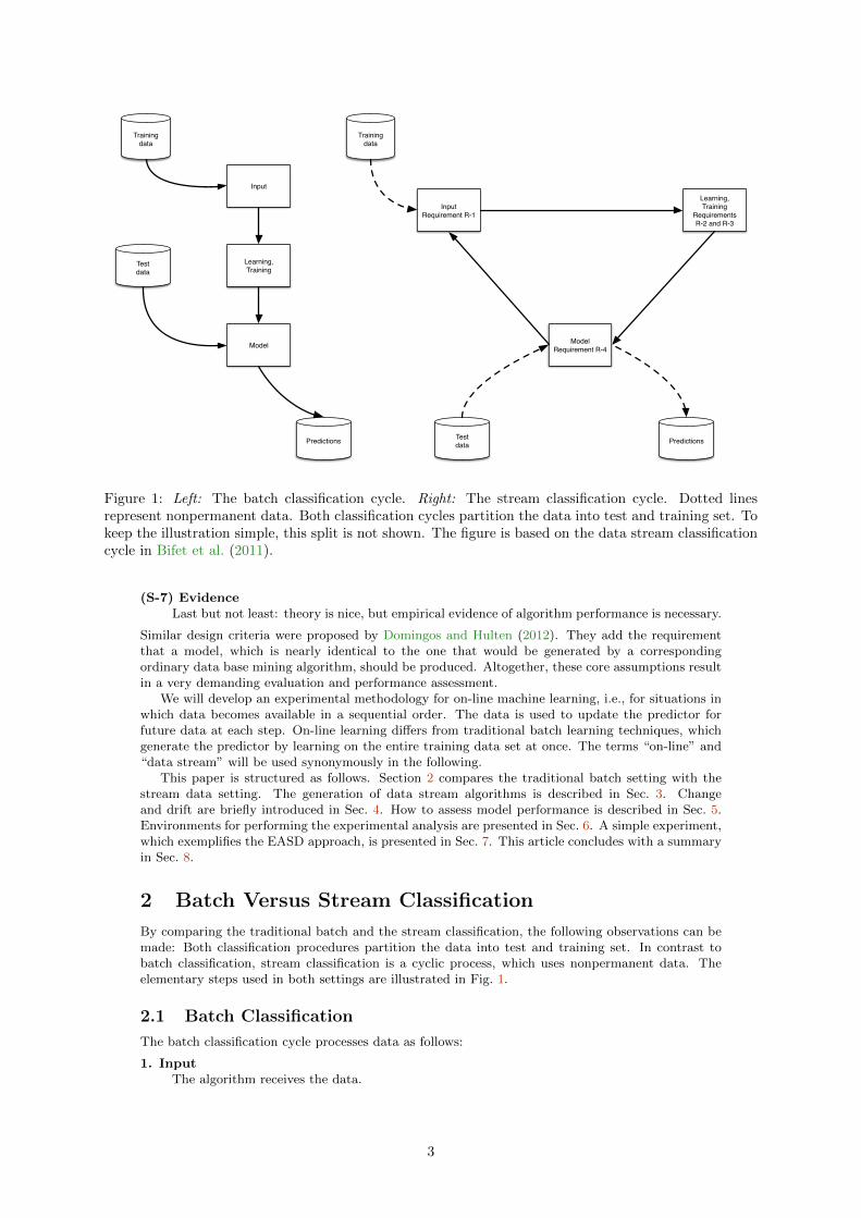
Figure 1: Left: The batch classification cycle. Right: The stream classification cycle. Dotted linesrepresent nonpermanent data. Both classification cycles partition the data into test and training set. Tokeep the illustration simple, this split is not shown. The figure is based on the data stream classificationcycle in Bifet et al. (2011).

(S-7) EvidenceLast but not least: theory is nice, but empirical evidence of algorithm performance is necessary.

Similar design criteria were proposed by Domingos and Hulten (2012). They add the requirementthat a model, which is nearly identical to the one that would be generated by a correspondingordinary data base mining algorithm, should be produced. Altogether, these core assumptions resultin a very demanding evaluation and performance assessment.

We will develop an experimental methodology for on-line machine learning, i.e., for situations inwhich data becomes available in a sequential order. The data is used to update the predictor forfuture data at each step. On-line learning differs from traditional batch learning techniques, whichgenerate the predictor by learning on the entire training data set at once. The terms “on-line” and“data stream” will be used synonymously in the following.

This paper is structured as follows. Section 2 compares the traditional batch setting with thestream data setting. The generation of data stream algorithms is described in Sec. 3. Changeand drift are briefly introduced in Sec. 4. How to assess model performance is described in Sec. 5.Environments for performing the experimental analysis are presented in Sec. 6. A simple experiment,which exemplifies the EASD approach, is presented in Sec. 7. This article concludes with a summaryin Sec. 8.

2 Batch Versus Stream Classification

By comparing the traditional batch and the stream classification, the following observations can bemade: Both classification procedures partition the data into test and training set. In contrast tobatch classification, stream classification is a cyclic process, which uses nonpermanent data. Theelementary steps used in both settings are illustrated in Fig. 1.

2.1 Batch Classification

The batch classification cycle processes data as follows:

1. InputThe algorithm receives the data.

3

2. LearnThe algorithm processes the data and generates its own data structures (builds a model).

3. PredictThe algorithm predicts the class of unseen data using the test set.

2.2 Stream Classification

Data availability differs in the stream classification cycle. Additional restrictions have to be consid-ered (Bifet et al., 2011). Freely adapted from Bifet et al. (2011), the data stream processing can bedescribed as follows:

1. InputThe algorithm receives the next data from the stream. At his stage of the process, the followingrequirement has to be considered:

(R-1) Process only onceData stream data is accepted as they arrive. After inspection, the data is not available anymore. However, the algorithm itself is allowed to set up an archive (memory). For example,the algorithm can store a batch of data that is used by traditional, static algorithms. Dueto the limited amount of memory, the algorithm has to discard the data after a certaintime period.

2. LearnThe algorithm processes the data and updates its own data structures (updates the model). Athis stage of the process, the following requirements have to be considered:

(R-2) Limited Memory BudgetData stream algorithms allow processing data that are several times bigger than the work-ing memory. Memory can be classified as memory that is used to store running statisticsand memory that is used to store the current model.

(R-3) Limited Time BudgetRuntime complexity of the algorithms should be linear in the amount of data, i.e., thenumber of examples. Real-time processing requires that the algorithm process the dataquickly (or even faster) than they arrive.

3. PredictThe algorithm is able to receive the next data. If requested, it is also able to predict the classof unseen data. At his stage of the process, the following requirement has to be considered:

(R-4) Predict at any PointThe best model should be generated as efficiently as possible. The model is generateddirectly in memory by the algorithm as it processes incoming data.

3 Generating Data Stream Algorithms

The process of enabling ML algorithms to process large amount of data is called scaling (Dietterich,1997). In data mining, the wrapper and the adaptation approach are known for this task.

3.1 Wrapper

The maximum reuse of existing schemes is referred to as the wrapper approach. The wrapperapproach collects and pre-processes data so that traditional batch learners can be used for modelbuilding.

Bifet et al. (2011) list typical implementations of the wrapper approach: Chu and Zaniolo (2004)propose a boosting ensemble method, which is based on a dynamic sample-weight assignment scheme.They claim that this method is fast, makes light demands on memory resources, and is able to adaptto concept drift. Wang et al. (2010) introduce a framework for mining concept-drifting data streams.An ensemble of classification models, such as C4.5 (Quinlan, 1993) or naive Bayes, is trained fromsequential chunks of the data stream. The classifiers in the ensemble are weighted based on theirestimated classification accuracy on the test data under the time-evolving environment. Thus, theensemble approach improves both the efficiency in learning the model and the accuracy in performingclassification.

Wrapper approaches suffer from the following difficulties: (i) The selection of an appropriatetraining set sizes is problematic. (ii) The training time cannot be controlled. Only the batch sizescan be modified, which provides a mean for an indirect control of the training time.

4

3.2 Adaptation

The adaptation approach develops new methods, which are specially designed for the stream dataanalysis task. Adaptation comprehends the careful design of algorithms especially designed to fulfilldata mining and ML tasks on dynamic data. Adaptation algorithms can implement direct strategiesfor memory management and are usually more flexible than wrapper approaches. Bifet et al. (2011)list examples for adaptation algorithms from the following algorithm classes: decision trees, associa-tion rules, nearest neighbor methods, support vector machines, neural networks, and ensemble-basedmethods.

4 Change and Drift Detection

Changes in the data distribution play an important role in data stream analysis. This motivatedthe development of specialized techniques, e.g., change detection strategies (Lughofer and Sayed-Mouchaweh, 2015). The target value, which will be predicted by the model, is referred to as concept.Several changes over time may occur: A gradual concept change is referred to as a concept drift. Arapid concept change over time is referred to as a concept shift, and a change in the data distributionis referred to as a distribution or sample change.

Established methods from statistical process control, e.g., the cumulative sum (CUSUM) algo-rithm, can be used for change detection (Montgomery, 2008). Further methods comprehend thegeometric-moving-average (GMA) test or statistical hypothesis tests. Hypotheses tests are popular,because they are well-studied and can be implemented easily. They compare data from two streams.The null hypothesis H0 reads: both streams come from the same distribution. Then a hypothesistest, which is based on the difference of means µ1 and µ2 is performed, e.g., the Kolmogorov-Smirnov(KS) test.

Gama et al. (2004) developed a drift-detection method, which is based on the on-line error-rate.The training examples are presented in sequence. New training example are classified using the actualmodel. As long as the distribution is stationary, the classification error will decrease. If a changein the distribution occurs, the error will increase. The trace of the on-line error of the algorithm isobserved.

Further approaches, e.g., based on the exponential-weighted-moving-average (EWMA) were de-veloped (Ross et al., 2012). The reader is referred to Gustafsson (2001), who presents an overviewof change detection methods.

5 Assessing Model Performance

This section describes an experimental setting for the assessment of model performance. In Sec. 5.1performance criteria are introduced. The experimental evaluation of the model performance requiresdata. Strategies for obtaining test data are described in Sec. 5.2.

5.1 Performance Criteria

Elementary performance criteria for data stream algorithms are based on

P-1 time (speed)We consider the amount of time needed (i) to learn and (ii) to predict. If the time limit isreached, continuing the data processing will take longer or results will loose precision. Thisconsequence is not so hard as the space limit, because overriding the space limit will force thealgorithm to stop.

P-2 space (memory)A simple strategy for the handling space budget is to stop once the limit is reached. To continueprocessing if the the space limit is reached is to force the algorithm to discard parts of its data.

P-3 error rates (statistical measures)The prediction error is considered. Several error measures are available (Hyndman and Koehler,2006; Willmott and Matsuura, 2005).

Regarding classification, the following error measures are established. We will consider a binaryclassification test, e.g., a test that screens items for a certain feature. In this setting, the term“positive” corresponds with “identified” (the item has the feature) and “negative” correspondswith “rejected” (the item does not have the feature), i.e.,

• TP: true positive = correctly identified

• FP: false positive = incorrectly identified = α error of the first type

• TN: true negative = correctly rejected

5

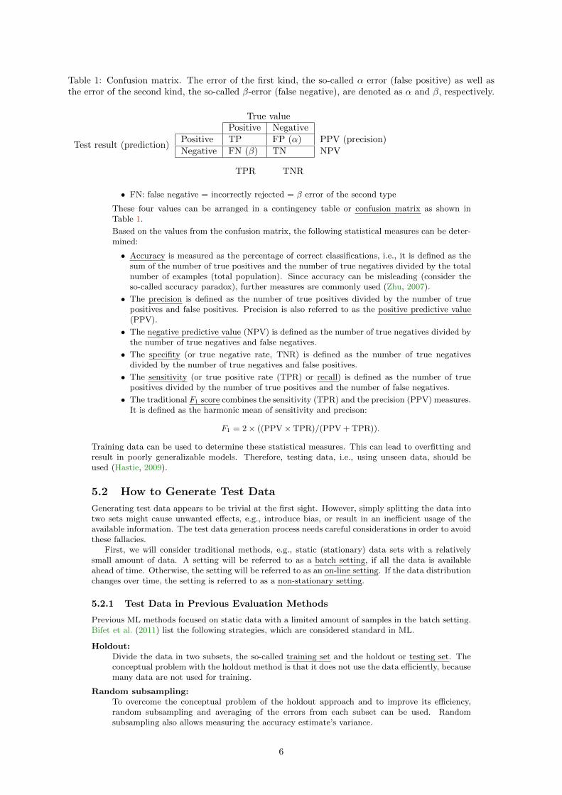
Table 1: Confusion matrix. The error of the first kind, the so-called α error (false positive) as well asthe error of the second kind, the so-called β-error (false negative), are denoted as α and β, respectively.

True valuePositive Negative

Test result (prediction)Positive TP FP (α) PPV (precision)Negative FN (β) TN NPV

TPR TNR

• FN: false negative = incorrectly rejected = β error of the second type

These four values can be arranged in a contingency table or confusion matrix as shown inTable 1.

Based on the values from the confusion matrix, the following statistical measures can be deter-mined:

• Accuracy is measured as the percentage of correct classifications, i.e., it is defined as thesum of the number of true positives and the number of true negatives divided by the totalnumber of examples (total population). Since accuracy can be misleading (consider theso-called accuracy paradox), further measures are commonly used (Zhu, 2007).

• The precision is defined as the number of true positives divided by the number of truepositives and false positives. Precision is also referred to as the positive predictive value(PPV).

• The negative predictive value (NPV) is defined as the number of true negatives divided bythe number of true negatives and false negatives.

• The specifity (or true negative rate, TNR) is defined as the number of true negativesdivided by the number of true negatives and false positives.

• The sensitivity (or true positive rate (TPR) or recall) is defined as the number of truepositives divided by the number of true positives and the number of false negatives.

• The traditional F1 score combines the sensitivity (TPR) and the precision (PPV) measures.It is defined as the harmonic mean of sensitivity and precison:

F1 = 2× ((PPV× TPR)/(PPV + TPR)).

Training data can be used to determine these statistical measures. This can lead to overfitting andresult in poorly generalizable models. Therefore, testing data, i.e., using unseen data, should beused (Hastie, 2009).

5.2 How to Generate Test Data

Generating test data appears to be trivial at the first sight. However, simply splitting the data intotwo sets might cause unwanted effects, e.g., introduce bias, or result in an inefficient usage of theavailable information. The test data generation process needs careful considerations in order to avoidthese fallacies.

First, we will consider traditional methods, e.g., static (stationary) data sets with a relativelysmall amount of data. A setting will be referred to as a batch setting, if all the data is availableahead of time. Otherwise, the setting will be referred to as an on-line setting. If the data distributionchanges over time, the setting is referred to as a non-stationary setting.

5.2.1 Test Data in Previous Evaluation Methods

Previous ML methods focused on static data with a limited amount of samples in the batch setting.Bifet et al. (2011) list the following strategies, which are considered standard in ML.

Holdout:Divide the data in two subsets, the so-called training set and the holdout or testing set. Theconceptual problem with the holdout method is that it does not use the data efficiently, becausemany data are not used for training.

Random subsampling:To overcome the conceptual problem of the holdout approach and to improve its efficiency,random subsampling and averaging of the errors from each subset can be used. Randomsubsampling also allows measuring the accuracy estimate’s variance.

6

Random subsampling suffers from the following disadvantage: If the training set contains manydata from one class, than the test set naturally contains only a few data from this class. Thisbias results in random subsampling violating the assumption that training and test sets areindependent.

Cross validation (CV):Cross validation (Arlot and Celisse, 2009) optimizes the use of data for training and testing.Every available data is used for training and testing. To avoid bias, stratified cross-validationcan be used.

Leave-one-out CV:is a special case of cross-validation, which is relatively expensive to perform if the model fit iscomplex. Leave-one-out CV is, in contrast to CV, completely deterministic. However, leave-one-out CV can fail, e.g., consider a classification situation with two classes, when data iscompletely random and 50 percent of the data belong to each class. The leave-one-out CVfails, because the majority vote is always wrong on the hold-out data and leave-one-out CVwill predict an accuracy of zero, although the expected accuracy is 50 percent.

The bootstrap:The bootstrap method (Efron and Tibshirani, 1993) generates a bootstrap sample by samplingwith replacement a training data set, which has the same size as the original data. The datathat are not in the training data set are used used for testing. The bootstrap can generatewrong results (in this case, they are too optimistic) in settings described for the leave-one-outCV.

Recommendations for choosing a suitable evaluation method are given in Kohavi (1995). Kleijnen(2008) discusses these methods in the context of simulation experiments.

5.2.2 Evaluation Procedures for Dynamic Data Stream Methods

In the dynamic data stream setting, plenty of data is available. The simple holdout strategy can beused without causing the problems mentioned in the batch setting. In contrast to the batch settings,large data sets for exact accuracy estimations can be used for testing without problems.

Holdout:The simplest approach is just holding out one (large) single reference data set during the wholelearning (training) phase. Using this holdout data set, the model can be evaluated periodically.This holdout data set can be generated using (i) old or (ii) new data, i.e., look-ahead data sets.The look-ahead method (Aggarwal, 2013) can give the model additional information (additionaltraining data) after the first testing phase is completed. This method is useful in situation whenconcept drift occurs.

In situations without any concept drift, a static holdout data set is adequate and better suited,because it does not introduce an additional source of randomness in the learning process.

Interleaved Test-Then-TrainIn addition to the holdout method, the interleaved test-then-train method was proposed forevaluating data stream algorithms (Bifet et al., 2010). Each new data can be used to test themodel before it is used for training. Advantages of this method are: (i) The model is tested onunknown data, (ii) each datum is used for testing and training, and (iii) the accuracy over timeis smooth, because each individual new data will become less significant to the overall average(the sample size is increasing).

Interleaved test-then-train methods obscure the differences between training and testing peri-ods. The true accuracy might be biased, because algorithms will be punished for early mistakes.This effect cancels out over time.

5.3 Analysis

A graphical plot (accuracy versus number of training samples) is the most common way presentingresults. Very often, the comparison of two algorithms is based on graphical comparisons by visualizingtrends (e.g., accuracy) over time. Bifet et al. (2011) describe the situation as follows:

”Most often this is determined from a single holdout run, and with an independent test setcontaining 300 thousand examples or less. It is rare to see a serious attempt at quantifyingthe significance of results with confidence intervals or similar checks.”

This situation appears to be similar to the situation for experimental algorithmics a decade ago,which was described in Sec. 1. To obtain reliable results, statistical measures such as the standarderror of results, are recommended. Useful approaches were described by Demsar (2006). For example,

7

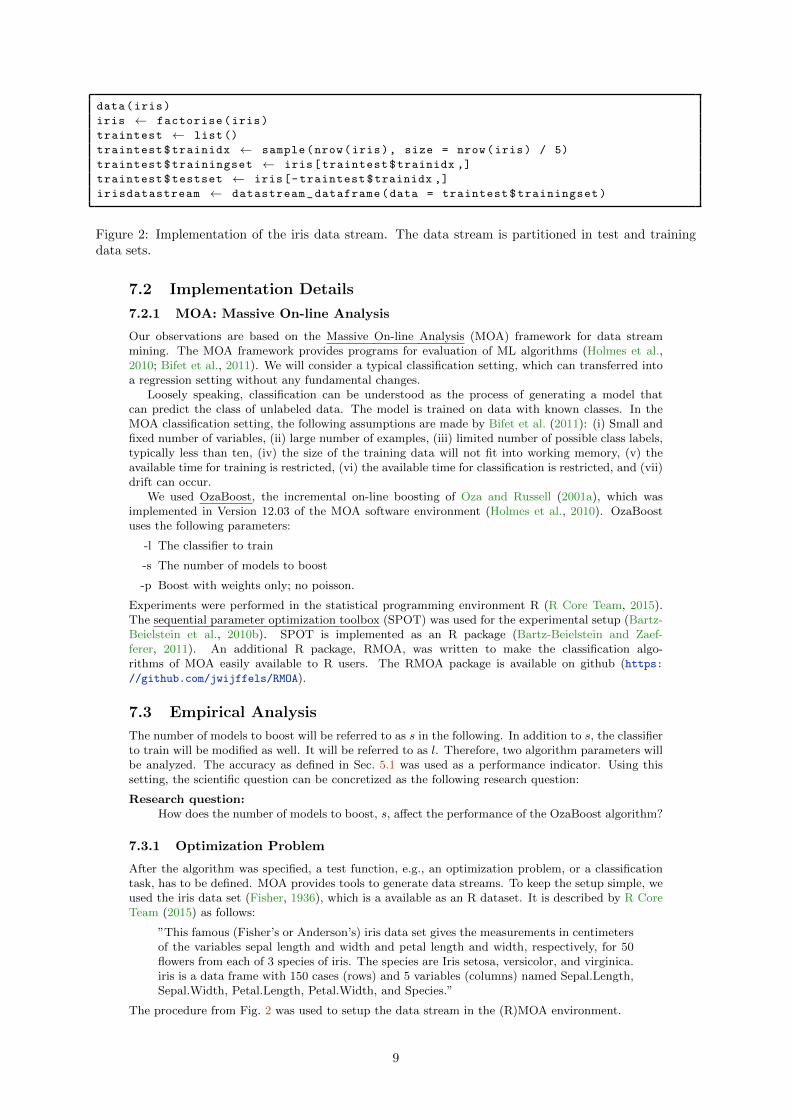
McNemar’s test can be used to measure the agreement between competing algorithms on each testdata (Dietterich, 1998). The statistical analysis should be accompanied by a comprehensive reportingscheme, which includes the relevant details for understanding and possible replication of the findings.The experimental analysis of data stream classification is subject of current research. Only a fewpublications that perform an extensive statistical analyis are available. Bifet et al. (2011) claim thatpaper Domingos and Hulten (2000) is the best analysis so far.

Fortunately, the open source framework for data stream mining MOA, which includes a collectionof machine learning algorithms (classification, regression, clustering, outlier detection, concept driftdetection and recommender systems) and tools for evaluation, is available and provides tools for anextensive experimental analysis (Holmes et al., 2010).

6 Environments and Data Sources

6.1 Real-world Data Stream Computing Environments

Computing environments can be classified as follows: (i) Sensor networks. In this setting, only a fewhundred kilobytes of memory are available. (ii) Handheld computer, which provide several megabytesof memory, (iii) Single-board computers, i.e., computers that are built on a single circuit board. Thecomponents such as microprocessor(s), memory, or input/output are located on this board. Single-board computers can be used as embedded computer controllers, and (iv) servers, which provideseveral gigabytes of RAM, e.g., 64 GB.

6.2 Simulators for Data Stream Analysis

Random data stream simulators are a valuable tool for the experimental analysis of data streamalgorithms. For our experiments in Sec. 7 a static data set, which contained pre-assigned classlabels, was used to simulate a real-world data stream environment. Consider a data set of size n,which is partitioned in training and test data sets with ntrain: number of examples used for trainingbefore an evaluation is performed on the test set. 2. ntest: size of the test set. Using naive Bayes orHoeffding trees, a model is built using the first ntrain instances for training. Prediction is performedon each of the remaining ntest instances. The test data is used to incrementally update the modelbuilt. This on-line stream setting allows the estimation of the model accuracy on an ongoing basis,because the results (class labels) are known in advance.

The open source framework for data stream mining MOA (Holmes et al., 2010) is able to generatea few thousand examples up to several hundred thousand examples per second. Additional noise canslow down the speed, because it requires the generation of random numbers.

7 A Simple Experiment in the EASD Framework

7.1 The Scientific Question

Before experimental runs are performed, the scientific question, which motivates the experiments,should be clearly stated. To exemplify the EASD approach, the following task is considered:

Machine learning methods, which combine multiple models to improve prediction accuracy, arecalled ensemble data mining algorithms. Diversity of the different models is necessary to reach thisperformance gain compared to individual models. If ensemble members always agree, the ensembledoes not provide an extra benefit. Errors of one ensemble member can be corrected by other membersof the ensemble.

Each individual ML algorithm requires the specification of some parameters, e.g., the splittingcriterion for regression trees or the order of linear models. Building ensembles requires the speci-fication of additional algorithm parameters, e.g., the number of ensemble members. The scientificquestion can be formulated as follows:

Scientific question:How does the number of models to boost affect the performance of on-line learning algorithms?

To set up experiments, a specific algorithm (or a set of algorithms) has to be selected. Oza etal. presented a simple on-line bagging and boosting algorithm, OzaBoost (Oza and Russell, 2001b,a;Oza). OzaBoost combines multiple learned base models with the aim of improving generalizationperformance. OzaBoost implements an on-line version of these ensemble learners, which have beenused primarily in batch mode. The effect of the number of models to boost on the algorithmperformance is an important research question, which will be analyzed in the following experiments.Therefore, the experimental setup as well as the implementation details have to be specified further.

8

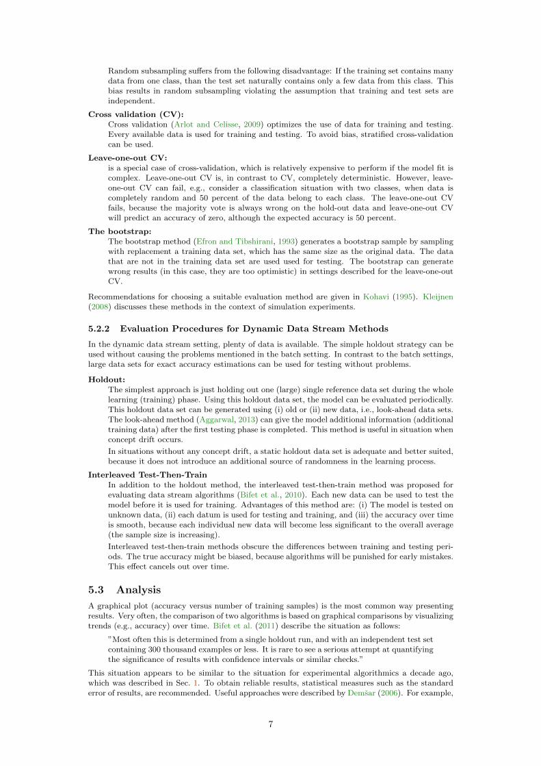
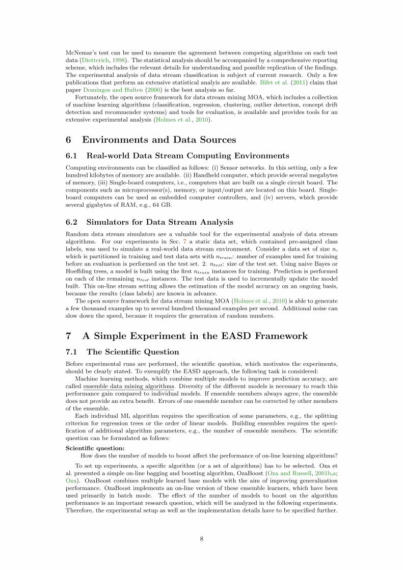
data(iris)

iris ← factorise(iris)

traintest ← list()

traintest$trainidx ← sample(nrow(iris), size = nrow(iris) / 5)

traintest$trainingset ← iris[traintest$trainidx ,]

traintest$testset ← iris[-traintest$trainidx ,]

irisdatastream ← datastream_dataframe(data = traintest$trainingset)

Figure 2: Implementation of the iris data stream. The data stream is partitioned in test and trainingdata sets.

7.2 Implementation Details

7.2.1 MOA: Massive On-line Analysis

Our observations are based on the Massive On-line Analysis (MOA) framework for data streammining. The MOA framework provides programs for evaluation of ML algorithms (Holmes et al.,2010; Bifet et al., 2011). We will consider a typical classification setting, which can transferred intoa regression setting without any fundamental changes.

Loosely speaking, classification can be understood as the process of generating a model thatcan predict the class of unlabeled data. The model is trained on data with known classes. In theMOA classification setting, the following assumptions are made by Bifet et al. (2011): (i) Small andfixed number of variables, (ii) large number of examples, (iii) limited number of possible class labels,typically less than ten, (iv) the size of the training data will not fit into working memory, (v) theavailable time for training is restricted, (vi) the available time for classification is restricted, and (vii)drift can occur.

We used OzaBoost, the incremental on-line boosting of Oza and Russell (2001a), which wasimplemented in Version 12.03 of the MOA software environment (Holmes et al., 2010). OzaBoostuses the following parameters:

-l The classifier to train

-s The number of models to boost

-p Boost with weights only; no poisson.

Experiments were performed in the statistical programming environment R (R Core Team, 2015).The sequential parameter optimization toolbox (SPOT) was used for the experimental setup (Bartz-Beielstein et al., 2010b). SPOT is implemented as an R package (Bartz-Beielstein and Zaef-ferer, 2011). An additional R package, RMOA, was written to make the classification algo-rithms of MOA easily available to R users. The RMOA package is available on github (https://github.com/jwijffels/RMOA).

7.3 Empirical Analysis

The number of models to boost will be referred to as s in the following. In addition to s, the classifierto train will be modified as well. It will be referred to as l. Therefore, two algorithm parameters willbe analyzed. The accuracy as defined in Sec. 5.1 was used as a performance indicator. Using thissetting, the scientific question can be concretized as the following research question:

Research question:How does the number of models to boost, s, affect the performance of the OzaBoost algorithm?

7.3.1 Optimization Problem

After the algorithm was specified, a test function, e.g., an optimization problem, or a classificationtask, has to be defined. MOA provides tools to generate data streams. To keep the setup simple, weused the iris data set (Fisher, 1936), which is a available as an R dataset. It is described by R CoreTeam (2015) as follows:

”This famous (Fisher’s or Anderson’s) iris data set gives the measurements in centimetersof the variables sepal length and width and petal length and width, respectively, for 50flowers from each of 3 species of iris. The species are Iris setosa, versicolor, and virginica.iris is a data frame with 150 cases (rows) and 5 variables (columns) named Sepal.Length,Sepal.Width, Petal.Length, Petal.Width, and Species.”

The procedure from Fig. 2 was used to setup the data stream in the (R)MOA environment.

9

set.seed (123)

ctrl ← MOAoptions(model = "NaiveBayes")

nbModel ← NaiveBayes(control=ctrl)

nbModelTrain ← trainMOA(model = nbModel

,Species ~ Sepal.Length +

Sepal.Width + Petal.Length + Petal.Width

,data = irisdatastream)

nbScores ← predict(nbModelTrain ,

newdata=traintest$testset[

, c("Sepal.Length","Sepal.Width"

,"Petal.Length","Petal.Width")]

,type="response")

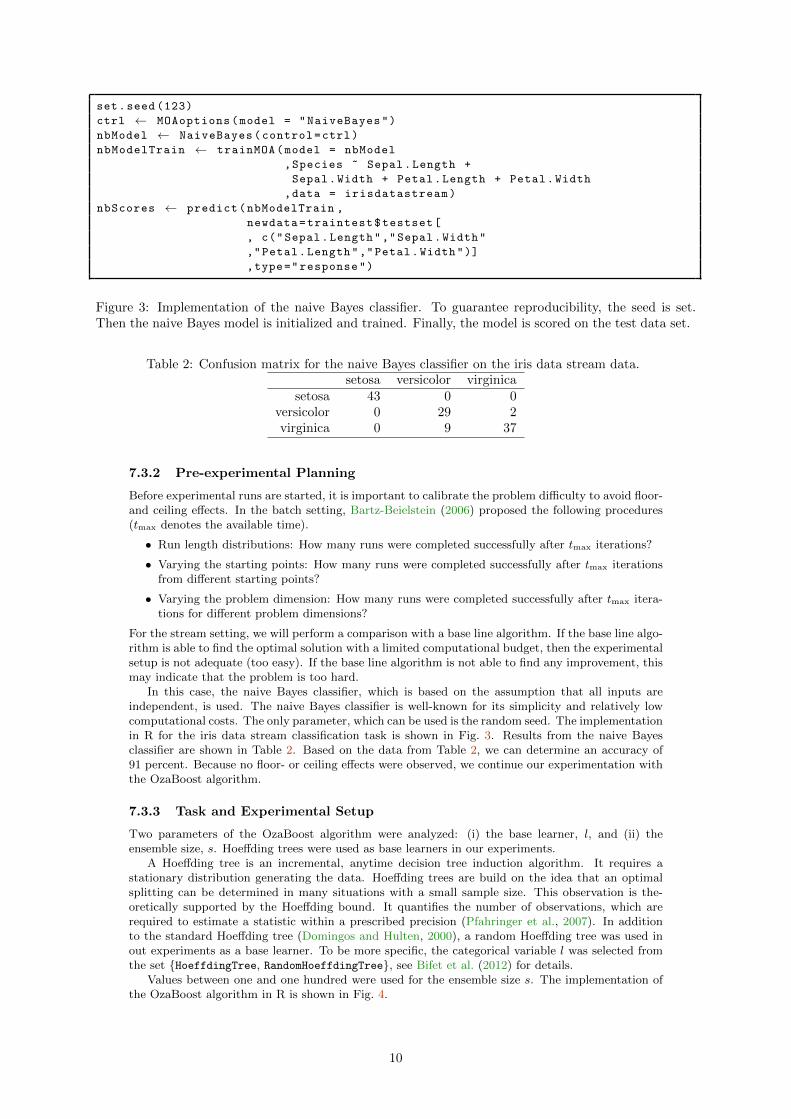
Figure 3: Implementation of the naive Bayes classifier. To guarantee reproducibility, the seed is set.Then the naive Bayes model is initialized and trained. Finally, the model is scored on the test data set.

Table 2: Confusion matrix for the naive Bayes classifier on the iris data stream data.setosa versicolor virginica

setosa 43 0 0versicolor 0 29 2virginica 0 9 37

7.3.2 Pre-experimental Planning

Before experimental runs are started, it is important to calibrate the problem difficulty to avoid floor-and ceiling effects. In the batch setting, Bartz-Beielstein (2006) proposed the following procedures(tmax denotes the available time).

• Run length distributions: How many runs were completed successfully after tmax iterations?

• Varying the starting points: How many runs were completed successfully after tmax iterationsfrom different starting points?

• Varying the problem dimension: How many runs were completed successfully after tmax itera-tions for different problem dimensions?

For the stream setting, we will perform a comparison with a base line algorithm. If the base line algo-rithm is able to find the optimal solution with a limited computational budget, then the experimentalsetup is not adequate (too easy). If the base line algorithm is not able to find any improvement, thismay indicate that the problem is too hard.

In this case, the naive Bayes classifier, which is based on the assumption that all inputs areindependent, is used. The naive Bayes classifier is well-known for its simplicity and relatively lowcomputational costs. The only parameter, which can be used is the random seed. The implementationin R for the iris data stream classification task is shown in Fig. 3. Results from the naive Bayesclassifier are shown in Table 2. Based on the data from Table 2, we can determine an accuracy of91 percent. Because no floor- or ceiling effects were observed, we continue our experimentation withthe OzaBoost algorithm.

7.3.3 Task and Experimental Setup

Two parameters of the OzaBoost algorithm were analyzed: (i) the base learner, l, and (ii) theensemble size, s. Hoeffding trees were used as base learners in our experiments.

A Hoeffding tree is an incremental, anytime decision tree induction algorithm. It requires astationary distribution generating the data. Hoeffding trees are build on the idea that an optimalsplitting can be determined in many situations with a small sample size. This observation is the-oretically supported by the Hoeffding bound. It quantifies the number of observations, which arerequired to estimate a statistic within a prescribed precision (Pfahringer et al., 2007). In additionto the standard Hoeffding tree (Domingos and Hulten, 2000), a random Hoeffding tree was used inout experiments as a base learner. To be more specific, the categorical variable l was selected fromthe set {HoeffdingTree, RandomHoeffdingTree}, see Bifet et al. (2012) for details.

Values between one and one hundred were used for the ensemble size s. The implementation ofthe OzaBoost algorithm in R is shown in Fig. 4.

10

ozaModel← OzaBoost(baseLearner = l , ensembleSize = s)

ozaModelTrain ← trainMOA(model = ozaModel

,formula = Species ~ Sepal.Length +

Sepal.Width + Petal.Length

,data = irisdatastream)

ozaScores ← predict(ozaModelTrain

,newdata = traintest$testset[, c("Sepal.Length"

,"Sepal.Width"

,"Petal.Length"

,"Petal.Width")]

,type = "response")

Figure 4: Implementation of the OzaBoost model.

0.0

2.5

5.0

7.5

10.0

0.4 0.6 0.8y

dens

ity

learner

0

1

●

●●

●

●

●

0.4

0.6

0.8

0 1learner

y

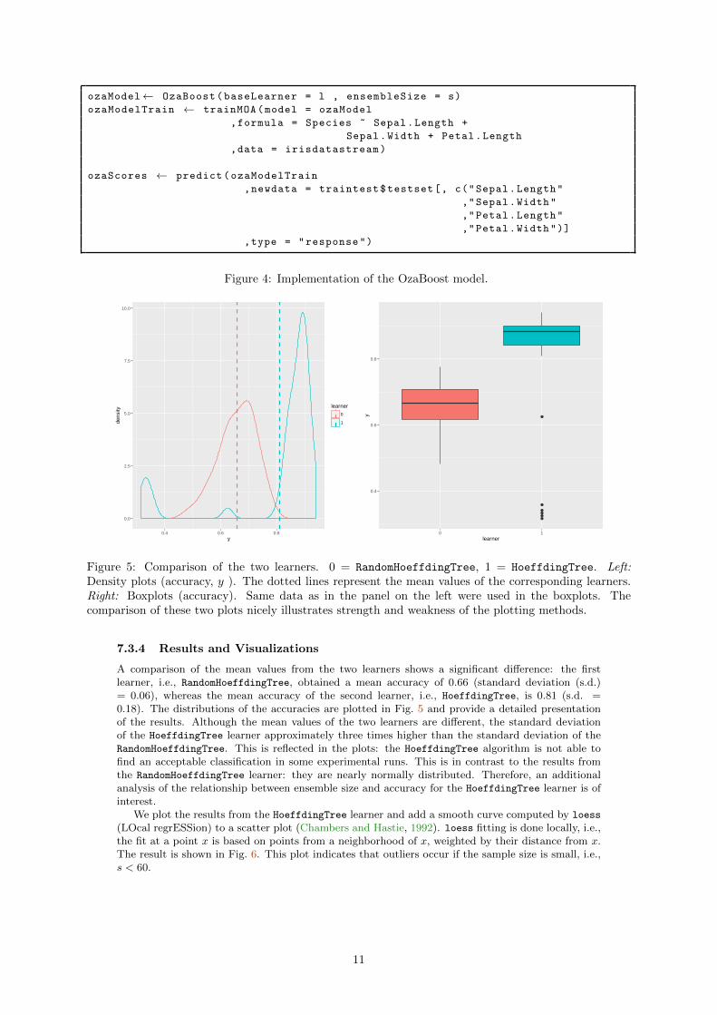
Figure 5: Comparison of the two learners. 0 = RandomHoeffdingTree, 1 = HoeffdingTree. Left:Density plots (accuracy, y ). The dotted lines represent the mean values of the corresponding learners.Right: Boxplots (accuracy). Same data as in the panel on the left were used in the boxplots. Thecomparison of these two plots nicely illustrates strength and weakness of the plotting methods.

7.3.4 Results and Visualizations

A comparison of the mean values from the two learners shows a significant difference: the firstlearner, i.e., RandomHoeffdingTree, obtained a mean accuracy of 0.66 (standard deviation (s.d.)= 0.06), whereas the mean accuracy of the second learner, i.e., HoeffdingTree, is 0.81 (s.d. =0.18). The distributions of the accuracies are plotted in Fig. 5 and provide a detailed presentationof the results. Although the mean values of the two learners are different, the standard deviationof the HoeffdingTree learner approximately three times higher than the standard deviation of theRandomHoeffdingTree. This is reflected in the plots: the HoeffdingTree algorithm is not able tofind an acceptable classification in some experimental runs. This is in contrast to the results fromthe RandomHoeffdingTree learner: they are nearly normally distributed. Therefore, an additionalanalysis of the relationship between ensemble size and accuracy for the HoeffdingTree learner is ofinterest.

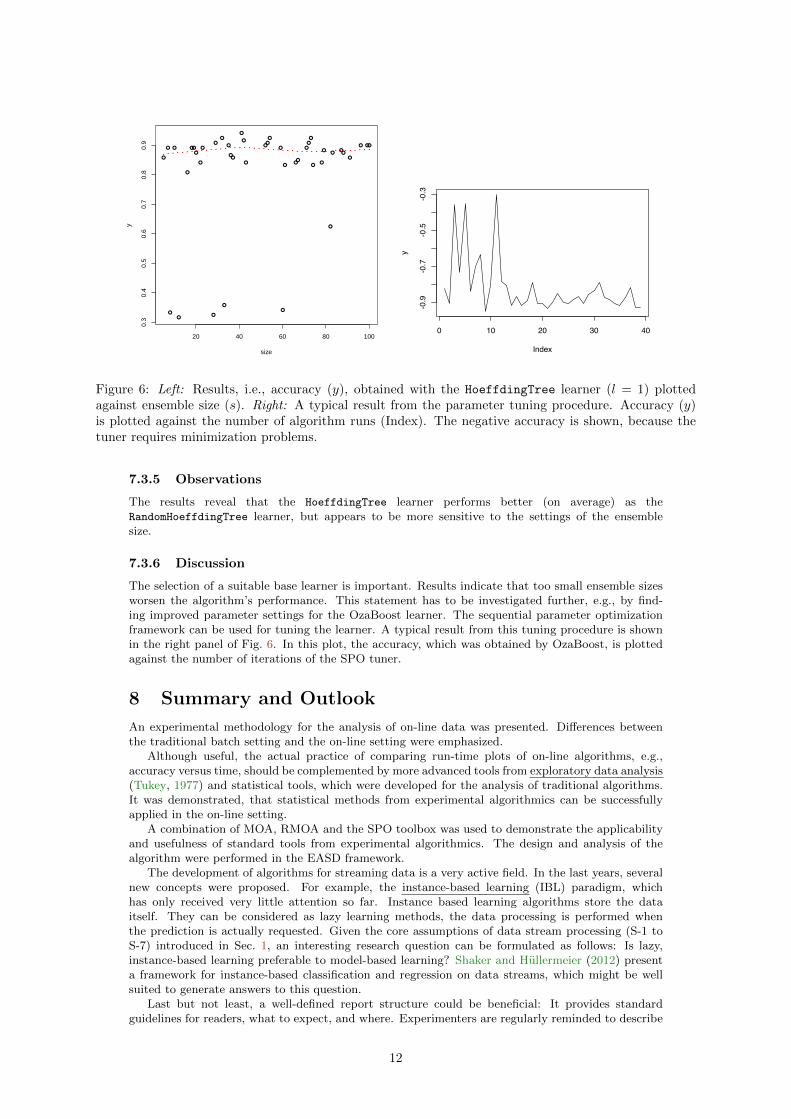
We plot the results from the HoeffdingTree learner and add a smooth curve computed by loess

(LOcal regrESSion) to a scatter plot (Chambers and Hastie, 1992). loess fitting is done locally, i.e.,the fit at a point x is based on points from a neighborhood of x, weighted by their distance from x.The result is shown in Fig. 6. This plot indicates that outliers occur if the sample size is small, i.e.,s < 60.

11

●

●

●

●

●

●

●●

●

●

●

●

●

●

●

●

●●

●

●

●

●●

●

●

●

●●●

●

●

●

●●

●

●

●●●

●

● ●●

20 40 60 80 100

0.3

0.4

0.5

0.6

0.7

0.8

0.9

size

y

0 10 20 30 40

-0.9

-0.7

-0.5

-0.3

Index

y

Figure 6: Left: Results, i.e., accuracy (y), obtained with the HoeffdingTree learner (l = 1) plottedagainst ensemble size (s). Right: A typical result from the parameter tuning procedure. Accuracy (y)is plotted against the number of algorithm runs (Index). The negative accuracy is shown, because thetuner requires minimization problems.

7.3.5 Observations

The results reveal that the HoeffdingTree learner performs better (on average) as theRandomHoeffdingTree learner, but appears to be more sensitive to the settings of the ensemblesize.

7.3.6 Discussion

The selection of a suitable base learner is important. Results indicate that too small ensemble sizesworsen the algorithm’s performance. This statement has to be investigated further, e.g., by find-ing improved parameter settings for the OzaBoost learner. The sequential parameter optimizationframework can be used for tuning the learner. A typical result from this tuning procedure is shownin the right panel of Fig. 6. In this plot, the accuracy, which was obtained by OzaBoost, is plottedagainst the number of iterations of the SPO tuner.

8 Summary and Outlook

An experimental methodology for the analysis of on-line data was presented. Differences betweenthe traditional batch setting and the on-line setting were emphasized.

Although useful, the actual practice of comparing run-time plots of on-line algorithms, e.g.,accuracy versus time, should be complemented by more advanced tools from exploratory data analysis(Tukey, 1977) and statistical tools, which were developed for the analysis of traditional algorithms.It was demonstrated, that statistical methods from experimental algorithmics can be successfullyapplied in the on-line setting.

A combination of MOA, RMOA and the SPO toolbox was used to demonstrate the applicabilityand usefulness of standard tools from experimental algorithmics. The design and analysis of thealgorithm were performed in the EASD framework.

The development of algorithms for streaming data is a very active field. In the last years, severalnew concepts were proposed. For example, the instance-based learning (IBL) paradigm, whichhas only received very little attention so far. Instance based learning algorithms store the dataitself. They can be considered as lazy learning methods, the data processing is performed whenthe prediction is actually requested. Given the core assumptions of data stream processing (S-1 toS-7) introduced in Sec. 1, an interesting research question can be formulated as follows: Is lazy,instance-based learning preferable to model-based learning? Shaker and Hullermeier (2012) presenta framework for instance-based classification and regression on data streams, which might be wellsuited to generate answers to this question.

Last but not least, a well-defined report structure could be beneficial: It provides standardguidelines for readers, what to expect, and where. Experimenters are regularly reminded to describe

12

the important details needed to understand and possibly replicate their experiments. They arealso urged to separate the outcome of fairly objective observing from subjective reasoning. Bartz-Beielstein and Preuss (2010) proposed organizing the presentation of experiments into seven parts,as follows:

ER-1: Research QuestionBriefly names the matter dealt with, the (possibly very general) objective, preferably in onesentence. This is used as the report’s “headline” and related to the primary model.

ER-2: Pre-experimental planningSummarizes the first—possibly explorative—program runs, leading to task and setup (ER-3and ER-4). Decisions on employed benchmark problems or performance measures should betaken according to the data collected in preliminary runs. The report on pre-experimentalplanning should also include negative results, e.g., modifications to an algorithm that did notwork or a test problem that turned out to be too hard, if they provide new insight.

ER-3: TaskConcretizes the question in focus and states scientific claims and derived statistical hypothesesto test. Note that one scientific claim may require several, sometimes hundreds, of statisticalhypotheses. In case of a purely explorative study, as with the first test of a new algorithm,statistical tests may not be applicable. Still, the task should be formulated as precisely aspossible. This step is related to the experimental model.

ER-4: SetupSpecifies problem design and algorithm design, including the investigated algorithm, the con-trollable and the fixed parameters, and the chosen performance measuring. The informationprovided in this part should be sufficient to replicate an experiment.

ER-5: Results/VisualizationGives raw or produced (filtered) data on the experimental outcome and additionally providesbasic visualizations where meaningful. This is related to the data model.

ER-6: ObservationsDescribes exceptions from the expected, or unusual patterns noticed, with- out subjectiveassessment or explanation. As an example, it may be worth- while to look at parameterinteractions. Additional visualizations may help to clarify what happens.

ER-7: DiscussionDecides about the hypotheses specified in ER-3, and provides necessarily subjective interpre-tations of the recorded observations. Also places the results in a wider context. The leadingquestion here is: What did we learn?

This report methodology, which is also described and exemplified in Preuss (2015), is an integralpart of the EASD framework.

References

C. C. Aggarwal. Managing and Mining Sensor Data. Springer US, 2013.

S. Arlot and A. Celisse. A survey of cross-validation procedures for model selection. ArXiv e-prints,July 2009.

R. Barr and B. Hickman. Reporting Computational Experiments with Parallel Algorithms: Issues,Measures, and Experts’ Opinions. ORSA Journal on Computing, 5(1):2–18, 1993.

R. Barr, B. Golden, J. Kelly, M. Rescende, and W. Stewart. Designing and Reporting on Computa-tional Experiments with Heuristic Methods. Journal of heuristics, 1(1):9–32, 1995.

T. Bartz-Beielstein. Experimental Analysis of Evolution Strategies—Overview and ComprehensiveIntroduction. Technical report, Nov. 2003.

T. Bartz-Beielstein. Experimental Research in Evolutionary Computation—The New Experimentalism.Natural Computing Series. Springer, Berlin, Heidelberg, New York, 2006.

T. Bartz-Beielstein and M. Preuss. The Future of Experimental Research. In T. Bartz-Beielstein,M. Chiarandini, L. Paquete, and M. Preuss, editors, Experimental Methods for the Analysis ofOptimization Algorithms, pages 17–46. Springer, Berlin, Heidelberg, New York, 2010.

T. Bartz-Beielstein and M. Zaefferer. SPOT Package Vignette. Technical report, 2011.

13

T. Bartz-Beielstein, C. Lasarczyk, and M. Preu. Sequential Parameter Optimization. In B. McKayet al., editors, Proceedings 2005 Congress on Evolutionary Computation (CEC’05), Edinburgh,Scotland, pages 773–780, Piscataway NJ, 2005. IEEE Press.

T. Bartz-Beielstein, M. Chiarandini, L. Paquete, and M. Preuss, editors.Experimental Methods for the Analysis of Optimization Algorithms. Springer, Berlin, Hei-delberg, New York, 2010a.

T. Bartz-Beielstein, C. Lasarczyk, and M. Preuss. The Sequential Parameter Optimization Toolbox.In T. Bartz-Beielstein, M. Chiarandini, L. Paquete, and M. Preuss, editors, Experimental Methodsfor the Analysis of Optimization Algorithms, pages 337–360. Springer, Berlin, Heidelberg, NewYork, 2010b.

E. W. Benfatti. A Study of Parameters Optimization to Tuning of MAPREDUCE/HADOOP, 2012.

A. Bifet, G. Holmes, R. Kirkby, and B. Pfahringer. MOA: Massive Online Analysis. J. Mach. Learn.Res., 11:1601–1604, Mar. 2010.

A. Bifet, G. Holmes, R. Kirkby, and B. Pfahringer. Data Stream Mining. pages 1–185, May 2011.

A. Bifet, R. Kirkby, P. Kranen, and P. Reutemann. Massive online analysis -Manual, Mar. 2012.

G. Cattaneo and G. Italiano. Algorithm engineering. ACM Comput. Surv., 31(3):3, 1999.

J. M. Chambers and T. J. Hastie, editors. Statistical Models in S. Statistical Models in S. Wadsworthand Brooks/Cole, Pacific Grove, CA, 1992.

F. Chu and C. Zaniolo. Fast and Light Boosting for Adaptive Mining of Data Streams. In ParallelProblem Solving from Nature - PPSN XIII - 13th International Conference, Ljubljana, Slovenia,September 13-17, 2014. Proceedings, pages 282–292. Springer Berlin Heidelberg, Berlin, Heidel-berg, 2004.

P. R. Cohen. Empirical Methods for Artificial Intelligence. MIT Press, Cambridge MA, 1995.

J. Demsar. Statistical Comparisons of Classifiers over Multiple Data Sets. J. Mach. Learn. Res., 7:1–30, Dec. 2006.

T. G. Dietterich. Machine-Learning Research. AI Magazine, 18(4):97, Dec. 1997.

T. G. Dietterich. Approximate Statistical Tests for Comparing Supervised Classification LearningAlgorithms. Neural computation, 10(7):1895–1923, Oct. 1998.

P. Domingos and G. Hulten. Mining high-speed data streams. In the sixth ACM SIGKDDinternational conference, pages 71–80, New York, New York, USA, 2000. ACM Press.

P. Domingos and G. Hulten. A General Framework for Mining Massive Data Streams. Journal ofComputational and Graphical Statistics, 12(4):945–949, Jan. 2012.

B. Efron and R. J. Tibshirani. An Introduction to the Bootstrap. Chapman and Hall, London, 1993.

A. E. Eiben and M. Jelasity. A Critical Note on Experimental Research Methodology in EC. InProceedings of the 2002 Congress on Evolutionary Computation (CEC’2002), pages 582–587, Pis-cataway NJ, 2002. IEEE.

R. A. Fisher. The use of multiple measurements in taxonomic problems. Annals Eugen., 7:179–188,1936.

J. Gama, P. Medas, G. Castillo, and P. Rodrigues. Learning with Drift Detection. In Parallel ProblemSolving from Nature - PPSN XIII - 13th International Conference, Ljubljana, Slovenia, September13-17, 2014. Proceedings, pages 286–295. Springer Berlin Heidelberg, Berlin, Heidelberg, 2004.

F. Gustafsson. Adaptive Filtering and Change Detection. Gustafsson: Adaptive. John Wiley &Sons, Ltd, Chichester, UK, Oct. 2001.

N. Hansen, A. Auger, S. Finck, and R. Ros. BBOB’09: Real-parameter black-box optimizationbenchmarking. Technical report, 2009.

T. Hastie. The elements of statistical learning : data mining, inference, and prediction. Springer,New York, 2nd ed. edition, 2009.

14

G. Holmes, B. Pfahringer, P. Kranen, T. Jansen, T. Seidl, and A. Bifet. MOA: Massive Online Analy-sis, a Framework for Stream Classification and Clustering. In International Workshop on HandlingConcept Drift in Adaptive Information Systems in conjunction with European Conference onMachine Learning and Principles and Practice of Knowledge Discovery in Databases ECMLPKDD, pages 3–16, 2010.

J. N. Hooker. Needed: An empirical science of algorithms. Operations research, 42(2):201–212, 1994.

J. N. Hooker. Testing Heuristics: We Have It All Wrong. Journal of heuristics, 1(1):33–42, 1996.

R. J. Hyndman and A. B. Koehler. Another look at measures of forecast accuracy. InternationalJournal of Forecasting, 22(4):679–688, Oct. 2006.

D. S. Johnson, C. R. Aragon, L. A. McGeoch, and C. Schevon. Optimization by Simulated Annealing:an Experimental Evaluation. Part I, Graph Partitioning. Operations research, 37(6):865–892, 1989.

D. S. Johnson, C. R. Aragon, L. A. McGeoch, and C. Schevon. Optimization by Simulated Anneal-ing: an Experimental Evaluation. Part II, Graph Coloring and Number Partitioning. Operationsresearch, 39(3):378–406, 1991.

J. P. C. Kleijnen. Design and analysis of simulation experiments. Springer, New York NY, 2008.

R. Kohavi. A Study of Cross-Validation and Bootstrap for Accuracy Estimation and Model Selection.pages 1–8, 1995.

E. Lughofer and M. Sayed-Mouchaweh. Adaptive and on-line learning in non-stationary environ-ments. Evolving Systems, 6(2):75–77, Feb. 2015.

C. C. McGeoch. Experimental Analysis of Algorithms. PhD thesis, Carnegie Mellon University,Pittsburgh PA, 1986.

C. C. McGeoch. A Guide to Experimental Algorithmics. Cambridge University Press, New York,NY, USA, 1st edition, 2012.

D. C. Montgomery. Statistical Quality Control. Wiley, 2008.

N. C. Oza. Online Bagging and Boosting. In 2005 IEEE International Conference on Systems, Manand Cybernetics.

N. C. Oza and S. Russell. Online bagging and boosting. In T. Jaakola and T. Richardson, editors,8th Insternational Workshop on Artificial Intelligence and Statistics, pages 105–112, 2001a.

N. C. Oza and S. Russell. Experimental comparisons of online and batch versions of bagging andboosting. In the seventh ACM SIGKDD international conference, pages 359–364, New York, NewYork, USA, 2001b. ACM Press.

B. Pfahringer, G. Holmes, and R. Kirkby. New Options for Hoeffding Trees. In AI 2007: Advancesin Artificial Intelligence, pages 90–99. Springer Berlin Heidelberg, Berlin, Heidelberg, Dec. 2007.

M. Preuss. Multimodal Optimization by Means of Evolutionary Algorithms. Natural ComputingSeries. Springer International Publishing, Cham, 2015.

J. R. Quinlan. C4.5: Programs for Machine Learning. Morgan Kaufmann Publishers Inc., San Fran-cisco, CA, USA, 1993.

R Core Team. R: A Language and Environment for Statistical Computing. R Foundation for Sta-tistical Computing, Vienna, Austria, 2015.

G. J. Ross, N. M. Adams, D. K. Tasoulis, and D. J. Hand. Exponentially weighted moving averagecharts for detecting concept drift. 33(2):191–198, Jan. 2012.

T. J. Santner, B. J. Williams, and W. I. Notz. The Design and Analysis of Computer Experiments.Springer, Berlin, Heidelberg, New York, 2003.

A. Shaker and E. Hullermeier. IBLStreams: a system for instance-based classification and regressionon data streams. Evolving Systems, 3(4):235–249, 2012.

P. N. Suganthan, N. Hansen, J. J. Liang, K. Deb, Y. P. Chen, A. Auger, and S. Tiwari. Problem Defi-nitions and Evaluation Criteria for the CEC 2005 Special Session on Real-Parameter Optimization.Technical report, Singapore, 2005.

15

J. W. Tukey. Explorative data analysis. Addison-Wesley, 1977.

H. Wang, P. S. Yu, and J. Han. Mining Concept-Drifting Data Streams. In Data Mining andKnowledge Discovery Handbook, pages 789–802. Springer US, Boston, MA, July 2010.

D. Whitley, K. Mathias, S. Rana, and J. Dzubera. Evaluating evolutionary algorithms. ArtificialIntelligence, 85(1–2):245–276, 1996.

C. J. Willmott and K. Matsuura. Advantages of the mean absolute error (MAE) over the root meansquare error (RMSE) in assessing average model performance. Clim Res, pages 1–4, Dec. 2005.

M. Zaefferer, T. Bartz-Beielstein, B. Naujoks, T. Wagner, and M. Emmerich. A Case Study on Multi-Criteria Optimization of an Event Detection Software under Limited Budgets. In R. C. Purshouseet al., editors, Evolutionary Multi-Criterion Optimization 7th International Conference, EMO,pages 756–770, Heidelberg, 2013. Springer.

X. Zhu. Knowledge Discovery and Data Mining: Challenges and Realities: Challenges and Realities.Gale virtual reference library. Information Science Reference, 2007.

16

CIplus Band 2/2016

EASD - Experimental Algorithmics for Streaming Data Prof. Dr. Thomas Bartz-Beielstein Institut für Informatik Fakultät für Informatik und Ingenieurwissenschaften Technische Hochschule Köln März 2016

Die Verantwortung für den Inhalt dieser Veröffentlichung liegt beim Autor.