1

Wagging: A learning approach which allows single layer perceptrons to outperform more

complex learning algorithms

Tim Andersen Tony Martinez Brigham Young University Brigham Young Universtiy

Provo, Utah Provo, Utah

Abstract:

Despite the well known inability of single layer perceptrons (SLPs) to learn arbitrary functions, SLPs often exhibitreasonable generalization performance on many problems of interest. However, because of the limitations of SLPsvery little effort has been made to improve their performance. In this paper we examine a method for improving theperformance of SLPs which we call "wagging" (weight averaging). This method involves training several differentSLPs on the same training data, and then averaging their weights to obtain a single SLP. We compare theperformance of the wagged SLP with other more complex learning algorithms on several data sets from real worldproblem domains. Surprisingly, the wagged SLP has better average generalization performance than any of theother learning algorithms on the problems tested. We provide analysis and explanations for this result. The analysisincludes looking at the performance characteristics of the standard delta rule training algorithm for SLPs and thecorrelation between training and test set scores as training progresses.

1. Introduction

For any given d dimensional classification problem a single layer perceptron (SLP) is limited to generating a d-

1 dimensional decision surface (hyperplane). For example, in a 2 dimensional input space an SLP is limited to

partitioning the input space with a single line. Therefore, any problem which can be completely solved by an SLP is

referred to as being linearly separable. The general consensus is that SLPs are not sufficiently powerful to perform

well on most types of classification problems (20). It is difficult to argue with this notion for two reasons. First, the

ratio of linearly separable problems to all possible problems quickly approaches zero as the problem dimension

increases. This would seem to indicate that an SLP is only applicable to an extremely small subset of the possible

problems. Second, most real world problems do not exhibit the characteristic of linear separability, and these are the

problems of primary interest. These two observations have motivated the development of learning algorithms which

are capable of generating more complex decision surfaces.

Unfortunately, coupled with an algorithm’s ability to generate more complex hypotheses is a higher likelihood

that the algorithm will overfit the data. So, utilizing a more complex learning algorithm, while perhaps guaranteeing

2

the ability to generate the solution we are looking for, does not necessarily guarantee that it will in fact generate a

good solution (one that performs well on unseen data). There are many methods available to help guard against the

problem of overfitting ([23], [15]), all of which are based upon either a complexity-accuracy tradeoff or the use of a

holdout set. However, overfitting avoidance is an enormously difficult problem, and no method for guarding against

overfitting has been shown to work well on all types of learning problems. The main difficulty lies in the proveable

fact that it is impossible to determine solely from the data what level of complexity is acceptable ([33], [26]). This

means that when testing a complex learning algorithm on a large variety of applications there will often be at least a

few applications which the algorithm performs poorly on due to overfitting. This tendency for a complex learning

algorithm to perform poorly on a few applications tends to counteract any exceptional performance that the

algorithm may have on other applications.

For example, in ([14]) the performance of c4.5 was compared against a very simple learning algorithm called

"1-rules", which is essentially a decision tree limited to 1 node. The paper showed that on many of the applications

which are commonly used in the machine learning community to test learning algorithms, 1-rules performs

equivalently to c4.5. And over all of the data sets tested the average generalization performance of c4.5 was not

significantly better than that of 1-rules.

In this paper we test and analyze a method for improving the performance of an SLP. In so doing we compare

two methods for improving this performance, bagging and weight averaging (wagging), against each other and

against other more complex machine learning methods on several real world problem domains. We make two

simple modifications to the standard perceptron training algorithm which significantly improves the generalization

performance of the SLP. The first modification is to save the best weight vector (in terms of training set accuracy)

produced during training, and the second is to average the weight vectors obtained from several different training

runs. Wagging is an attempt to average out the overfitting which occurs when using the most accurate weight vector

on the training set. These two modifications result in an average increase in generalization accuracy of

approximately four percent for an SLP on the data sets tested in this paper. This improvement is enough to boost the

performance of the SLP so that its average test set results are significantly better than all of the other machine

learning and neural network algorithms tested in this paper. The other learning algorithms include an MLP trained

with backpropogation, c4.5, id3, ib1, cn2, and others. These other algorithms are briefly described in section 2.

3

This is a surprising result, since the modifications which we make to the SLP only affect the final weight vector

generated by the training cycle, and do not actually increase the number of possible hypotheses which the SLP can

generate. There are several reasons for this dramatic improvement in generalization accuracy, which we discuss in

detail in section 4. As part of our analysis we look at the fluctuations in training and test errors as training

progresses, and across different training runs on the same training set. There are other papers which have explored

the learning and generalization traits of perceptrons [10, 3, 16, 12], but most of these use artificial data sets (learning

from a “teacher” perceptron) and limiting assumptions such as spherical weight constraints to obtain their results.

With this paper we concentrate on examining and improving the performance of SLPs on real world problems,

including problems which have varying amounts of noise and which are generally not linearly separable, and we

provide explanation and analysis of these improvements. We show empirically that picking the best weight vector

in terms of training set accuracy does not maximize test set accuracy.

Section 2 introduces the data sets and discusses the various machine learning and neural network algorithms

which are used in this paper for comparison purposes. Section 3 explores ways to improve the performance of SLPs.

Section 4 looks at the performance characteristics of the standard approach used to train SLPs, and why wagging

improves this performance. Section 5 discusses why a wagged SLP performs so well in comparison with other

learning algorithms. The conclusion and future work is given in section 6.

2. Algorithms and Data

tag full name attributes instances problem description

bc breast cancer 9 286 recurrence of breast cancer in treated patientsbcw breast cancer wisconsin 10 699 malignancy/nonmalignancy of breast tissue lumpbupa bupa liver disorders 7 345 blood tests thought to be sensitive to liver disorderscredit credit approval 15 690 credit card application approval dataecho echocardiogram 13 132 survival of heart attack victims after 1 yearsickeu sick-euthyroid 26 3163 presence/absence of sick-euthyroid in patienthypoth hypothyroid 26 3123 presence/absence of hypothyroidism in patiention ionosphere 35 351 classifcation of radar returns from ionosphere as "good" or "bad"promot promoter gene sequences 57 106 identification of promoter gene sequences in E. colisick sick 30 3772 presence/absence of thyroid disease in patientsonar sonar 61 208 identifying rocks and mines via reflected sonar signalsstger german credit numeric 24 1000 good/bad credit risk assesment of individualssthear statlog heart 13 270 presence/absence of heart disease in patienttic tic tac toe endgame 9 958 prediction of win/loss for x from all possible end game positionsvoting house votes 1984 16 435 predict party affiliation from house voting records

Table 1. Data sets.

Table 1 lists the data sets used in this paper. The first column gives the name (or tag) used to identify the data

4

set throughout the rest of this paper. The total number of attributes is listed in the third column, and the fourth

column gives the total number of examples contained in the data set. The last column describes the problem

domain. For the sake of simplicity we limited the data sets used in this paper to those with two output classes.

These data sets were obtained from the UCI machine learning database repository. All of these data sets, with the

exception of the tic-tac-toe data set, are based upon real world problem domains, and are more or less representative

of the types of classification problems that occur in the real world.

The scores we report throughout the rest of this paper for the other learning algorithms are taken from [34],

which is a comprehensive case study comparing the results of several machine learning algorithms across a large

variety of data sets. The results from this case study are averages obtained using 10-fold cross validation.

Generally, the various learning algorithms were tested using their default parameter settings. The exception to this is

with the multilayer network (which has no default parameter settings), which was run with several different

architectures and parameter settings and a performance measure was used to select between them.

All of the algorithms we test in this paper are trained/tested using 10-fold cross validation on the same data

splits that were used in [34]. This allows us to use the student t-test to calculate confidence levels and directly

compare the results of different learning algorithms on each data set. We then use the Wilcoxon statistical test to

calculate the confidence that one learning algorithm is better than another across all data sets and data splits.

Tag Full Name References

bp multilayer perceptron [@17]per linear threshold perceptron [@13, @14, @15, @16]c4 c4 [@8,@9]c4.5r c4.5 rules [@10]c4.5t c4.5 tree [@10]c4.5tp c4.5 tree pruned [@10]ib1 instance based 1 [@11, @12]id3 id3 [@10]mml IND v2.1 [@8,@9]smml IND v2.1 [@8,@9]cn2o ordered cn2 [@6, @7]cn2u unordered cn2 [@6, @7]

Table 2. Learning algorithms.

The learning algorithms we compare against are summarized in table 2. The first column lists the name which

we will use to refer to the corresponding learning algorithm throughout the rest of this paper. The second column

gives the usual name which people use to refer to the learning algorithm, and the last column lists some references

5

for each learning algorithm. A brief description of each type of learning algorithm follows.

A multilayer network is generally composed of multiple layers of nonlinear perceptrons. This type of network

is generally referred to as an MLP for multi-layer perceptron. Given enough nodes and layers, an MLP is

theoretically capable of learning any functional mapping by adjusting its weights. The major difficulty lies in the

setting of the large number of user defined parameters, such as the number of nodes, layers, interconnections

between nodes, learning rate, momentum, and so forth. In practice, it may be extremely difficult or even impossible

to determine optimal settings for all of the network parameters. Even with an optimal network architecture one must

still have enough training examples in order to properly constrain the network weights, and thus have a good chance

of the training process generating the desired (optimal) weight settings.

Decision trees are a well known learning model which have been extensively studied by many different

scientists in the machine learning community. Decision tree algorithms include c4.5, id3, and IND v2.1. A decision

tree is composed of possibly many decision nodes, all of which are connected by some path to the root node of the

tree. All examples enter the tree at the root decision node, which makes a decision, based upon the examples

attributes, about which branch to send the example on down the tree. The example is then passed down to the next

node on that branch, which makes a decision on which sub-branch to send the example down. This procedure

continues until the example reaches a leaf node of the tree, at which point a decision is made on the example's

classification.

Instance based learning algorithms are variants of the nearest neighbor classification algorithm. With a nearest

neighbor approach an example of an unknown class is classified the same as the closest example or set of closest

examples (where distance is generally measured in Euclidean terms) of known classification. The instance based

learning algorithms seek to decrease the amount of storage required by the standard nearest neighbor approach,

which normally saves the entire training set, while at the same time improving upon classification performance.

There are several variants to this approach. Due to space constraints we report only the results for ib1 since ib1

exhibited better overall performance than any of the other instance based learning algorithms on the data sets tested

in this paper .

The rule based learning algorithms are cn2 and c4.5r. c4.5r induces a decision tree as a precursor to generating

the rule list. The cn2 rule induction algorithm uses a modified search technique based on the AQ beam search

6

method. The original version of cn2 uses entropy as a search heuristic. With this heuristic cn2 performs

equivalently to id3 if the beam width is limited to 1. One of the advantages of rules is that they are generally

thought to be comprehensible by a human. However, this characteristic is only evident when the number of rules is

relatively small.

All of these learning algorithms are capable of generating hypotheses which are more complex than those

possible with an SLP. More complexity does not necessarily imply better generalization performance, however, as

we show with our results in the next section.

3 Improving the performance of an SLP

The output o of a perceptron for the kth input pattern is defined as

o =1 if wa xak + θ > 0

a∑

0 otherwise

⎧⎨⎪

⎩⎪(e1)

Where wa is the weight on input attribute axak is the value of attribute a for example kθ is an adjustable threshold

The standard training or weight update formula for a perceptron is the well known delta rule ([19]), which is

∆wa = c(tk − o)xak (3)

Where c is the learning ratetk is the target classification for example k

There are a few interesting things that one notices when running the standard delta rule training algorithm on

several different real world data sets. One of these observations is that on many of the data sets an SLP has

generalization performance which compares favorably to other, more complex learning algorithms. This is true even

on data sets which are not linearly separable. Even on many of the data sets where an SLP does not perform as well

as more complex methods, the main problem might not be that an SLP is inherently incapable of comparable

generalization performance, but that the training algorithm didn’t pick the best weight vector for generalization. For

example, it is possible for an SLP to achieve 100 percent accuracy on the promoter data set (table 12), but actual

generalization accuracy is usually much lower than this at around 87 percent. However, in section 4.3 we show that,

with a smarter choice for the weight vector, we are able to improve generalization accuracy to 91.55 percent on the

promoter data set.

7

Another interesting observation is that the best weight vector for one training run can differ significantly, at

least with a few of its weights, from the best weight vector from another training run, even if the training accuracies

of the two weight vectors are the same. This difference can be so significant that corresponding weights from the

two weight vectors can be of different sign. There will also generally be a few weights that are relatively stable

across multiple training runs on the same training set. The important question that one must answer when given

several different but equivalently performing (on the training set) weight vectors is which weight vector should one

choose?

Well, one should choose the best weight vector. Unfortuneately, it is impossible to say for certain which will be

the best, but a good choice might be the weight vector that, given the data and the training algorithm, is the most

probable. Since it is impossible to calculate the true probability of a weight vector, we must turn to ways that will

approximate its performance.

3.1 Bagging

One way to circumvent the problem of having to choose the single best weight vector is to train several different

SLP and use them all by having them vote for the output classification. This approach, termed “bagging”, has been

used with good success (5, 28, 18, 11). The standard bagging approach is defined as follows. Let B be the number

of predictors ϕ we wish to generate. First, B training sets are formed from the available training set T by taking

repeated random samples from T, then each of these training sets Tk is used to train a predictor ϕk. The output o of

the aggregation ϕB of all the ϕk predictors on input x is then

o = l j |∀i(i ≠ j → δk =1

B

∑ (l j ,ϕk (x)) > δk =1

B

∑ (li ,ϕk (x))) (4)

where li is the label for the ith output classδ is the Kronecker delta function

For two output classes, it is possible to avoid the case where there does not exist a class lj for which equation 4 holds

(in other words the case where there is a tie in the voting) by using an odd number of predictors. For more than two

output classes some method for resolving ties must be implemented. This can be arbitrary, based upon the prior

probabilities for each output class, or some other reasonable method.

It can be shown that the aggregate classifier ϕB will tend to have generalization performance which is at least as

8

good as the average performance of all the ϕk, assuming that the ϕk are reasonably good (better than random)

classifiers. The key to obtaining actual performance improvements with bagging is the degree of instability in the

ϕk. In other words, the ϕk must differ somewhat in the errors they exhibit for ϕB to improve classification over the

average classification performance.

When using random training set permutation between training iterations, there is no need to randomly resample

T to produce different ϕk for perceptrons trained with the standard delta rule method. Randomly permuting the data

with the perceptron training technique essentially guarantees that different training runs will produce different

solutions with correspondingly different errors. Bagging is therefore a natural fit for dealing with the many different

weight vectors that can be produced from multiple training runs on the same data for an SLP.

3.2 Wagging

The output of a linear perceptron on input x is defined as

o = wi xii

∑ (5)

where xi is the ith element of x.

Define wki to be the ith weight of the kth perceptron. The output of an aggregation of B linear perceptrons using

bagging is then

o = 1B wki xi

i∑

k∑ = 1

B wkik∑

⎛⎝⎜

⎞⎠⎟

xii

∑ (6)

Bagging multiple linear perceptrons is therefore equivalent to averaging their weights to obtain a single linear

perceptron. We term this approach “wagging” for

weight averaging.

Taking the average of all the available weight vectors is also one way to estimate the most probable weight

vector, since the average weight vector is a reasonable approximation to the most probable weight vector (given the

training algorithm and data). This approach has been tested with multilayer networks and been shown to work well

([29]).

Like wagging linear perceptrons, wagging multiple non-linear perceptrons is a form of bagging where only a

single weight vector, the average, need be stored. There are a number of different (but ultimately equivalent) ways

9

to view wagging of nonlinear perceptrons (hereafter referred to as just perceptrons) and its relation to bagging.

These are:

• Wagging with perceptrons is the same as bagging linear perceptrons, except that the final average output of the

linear perceptrons is thresholded to produce a discrete classification/output.

• Wagging with perceptrons is bagging where each network’s vote is weighted according to its activation,

whereas in the standard bagging approach for perceptrons each network’s vote has a weight of 1.

• Wagging is bagging where, instead of each unit voting for an output, each unit votes for the input weights.

There are two disadvantages to bagging. The main disadvantage of bagging is that it must store and run many

different predictors. Wagging solves this problem by requiring that only a single predictor/weight vector, the

average, be stored and run.

Another possible disadvantage of bagging for classification problems is that it does not take into account the

confidence of each predictor. With neural networks the activation of the net can loosely be viewed as the confidence

that the network has in its prediction. By using a single vote per predictor, it is possible for situations to arise where

several weak predictors outvote a few strong ones, which may not be desirable. Since wagging is equivalent to

bagging where each network votes its activation, wagging could improve generalization performance in cases where

network activation is correlated with confidence.

3.3 Bagging vs wagging

Table 3 compares the performance of bagging and wagging on 15 real world data sets. These results are

averages obtained using 10-fold cross validation on the available data. For each training set we generated 100

different SLPs by retraining 100 times using random permutations of the training set between each training iteration.

Weights were initially set to zero, and the maximum number of training iterations was set at 10,000 due to time

constraints. The best weight vector (BWV) was used from each training run as the final weight setting for each

SLP. The BWV was determined by pausing at the end of each training iteration and testing the SLP on the entire

training set and then saving the highest scoring weight vector. The rationale behind using the BWV rather than the

most recent weight vector will be explained in section 4. Equation 4 was used to obtain the estimated output for the

bagged SLPs. For the wagged SLP we used equation 7, which is derived from equation 6, to obtain the estimated

10

output of a single SLP with averaged weights.

o =1 if wki xi

i∑ > 0

k∑

0 otherwise

⎧⎨⎪

⎩⎪(7)

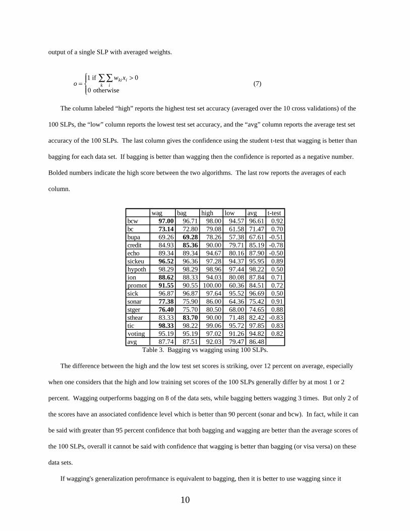
The column labeled “high” reports the highest test set accuracy (averaged over the 10 cross validations) of the

100 SLPs, the “low” column reports the lowest test set accuracy, and the “avg” column reports the average test set

accuracy of the 100 SLPs. The last column gives the confidence using the student t-test that wagging is better than

bagging for each data set. If bagging is better than wagging then the confidence is reported as a negative number.

Bolded numbers indicate the high score between the two algorithms. The last row reports the averages of each

column.

wag bag high low avg t-testbcw 97.00 96.71 98.00 94.57 96.61 0.92bc 73.14 72.80 79.08 61.58 71.47 0.70bupa 69.26 69.28 78.26 57.38 67.61 -0.51credit 84.93 85.36 90.00 79.71 85.19 -0.78echo 89.34 89.34 94.67 80.16 87.90 -0.50sickeu 96.52 96.36 97.28 94.37 95.95 0.89hypoth 98.29 98.29 98.96 97.44 98.22 0.50ion 88.62 88.33 94.03 80.08 87.84 0.71promot 91.55 90.55 100.00 60.36 84.51 0.72sick 96.87 96.87 97.64 95.52 96.69 0.50sonar 77.38 75.90 86.00 64.36 75.42 0.91stger 76.40 75.70 80.50 68.00 74.65 0.88sthear 83.33 83.70 90.00 71.48 82.42 -0.83tic 98.33 98.22 99.06 95.72 97.85 0.83voting 95.19 95.19 97.02 91.26 94.82 0.82avg 87.74 87.51 92.03 79.47 86.48

Table 3. Bagging vs wagging using 100 SLPs.

The difference between the high and the low test set scores is striking, over 12 percent on average, especially

when one considers that the high and low training set scores of the 100 SLPs generally differ by at most 1 or 2

percent. Wagging outperforms bagging on 8 of the data sets, while bagging betters wagging 3 times. But only 2 of

the scores have an associated confidence level which is better than 90 percent (sonar and bcw). In fact, while it can

be said with greater than 95 percent confidence that both bagging and wagging are better than the average scores of

the 100 SLPs, overall it cannot be said with confidence that wagging is better than bagging (or visa versa) on these

data sets.

If wagging's generalization perofrmance is equivalent to bagging, then it is better to use wagging since it

11

reduces the amount of storage and the amount of computation required during execution. It is also easier for a

human to analyze and understand a system composed of a single node, rather than one composed of a hundred

nodes.

3.4 Wagging vs other learning algorithms

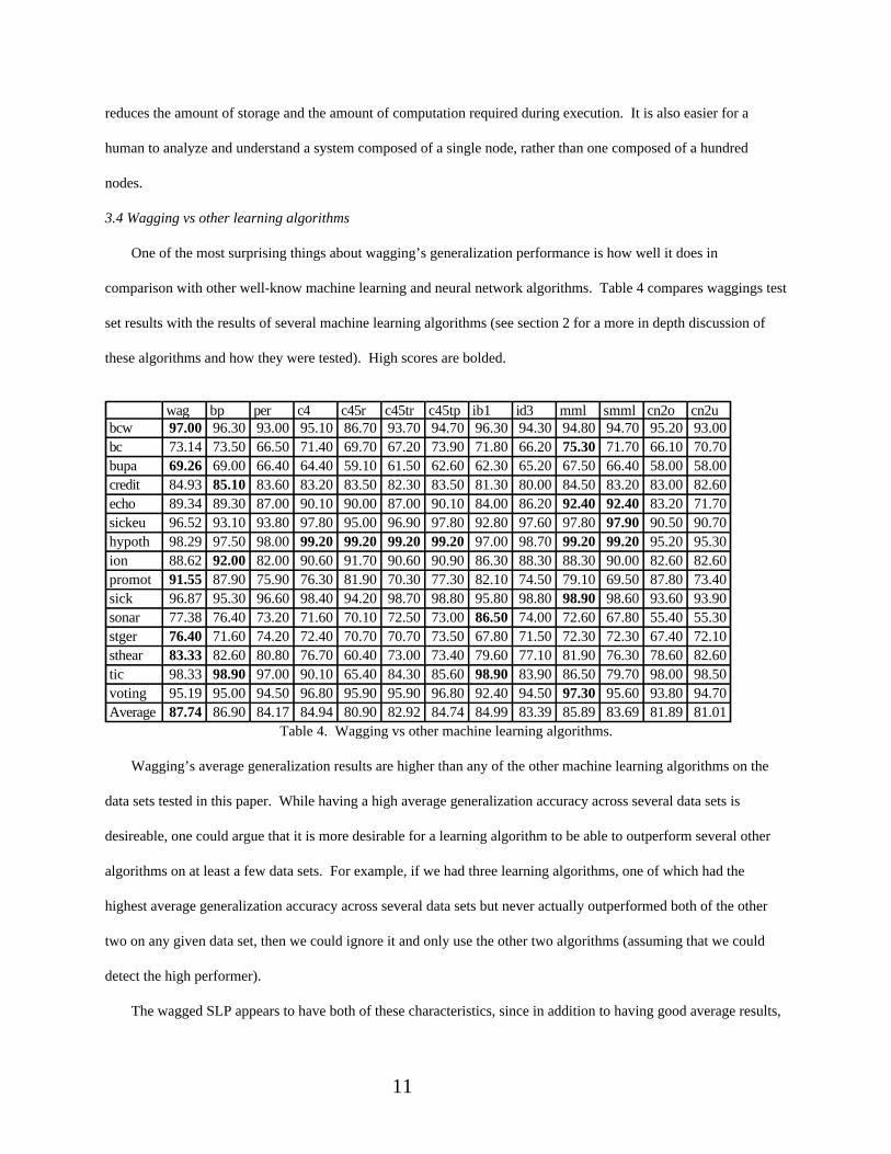
One of the most surprising things about wagging’s generalization performance is how well it does in

comparison with other well-know machine learning and neural network algorithms. Table 4 compares waggings test

set results with the results of several machine learning algorithms (see section 2 for a more in depth discussion of

these algorithms and how they were tested). High scores are bolded.

wag bp per c4 c45r c45tr c45tp ib1 id3 mml smml cn2o cn2ubcw 97.00 96.30 93.00 95.10 86.70 93.70 94.70 96.30 94.30 94.80 94.70 95.20 93.00bc 73.14 73.50 66.50 71.40 69.70 67.20 73.90 71.80 66.20 75.30 71.70 66.10 70.70bupa 69.26 69.00 66.40 64.40 59.10 61.50 62.60 62.30 65.20 67.50 66.40 58.00 58.00credit 84.93 85.10 83.60 83.20 83.50 82.30 83.50 81.30 80.00 84.50 83.20 83.00 82.60echo 89.34 89.30 87.00 90.10 90.00 87.00 90.10 84.00 86.20 92.40 92.40 83.20 71.70sickeu 96.52 93.10 93.80 97.80 95.00 96.90 97.80 92.80 97.60 97.80 97.90 90.50 90.70hypoth 98.29 97.50 98.00 99.20 99.20 99.20 99.20 97.00 98.70 99.20 99.20 95.20 95.30ion 88.62 92.00 82.00 90.60 91.70 90.60 90.90 86.30 88.30 88.30 90.00 82.60 82.60promot 91.55 87.90 75.90 76.30 81.90 70.30 77.30 82.10 74.50 79.10 69.50 87.80 73.40sick 96.87 95.30 96.60 98.40 94.20 98.70 98.80 95.80 98.80 98.90 98.60 93.60 93.90sonar 77.38 76.40 73.20 71.60 70.10 72.50 73.00 86.50 74.00 72.60 67.80 55.40 55.30stger 76.40 71.60 74.20 72.40 70.70 70.70 73.50 67.80 71.50 72.30 72.30 67.40 72.10sthear 83.33 82.60 80.80 76.70 60.40 73.00 73.40 79.60 77.10 81.90 76.30 78.60 82.60tic 98.33 98.90 97.00 90.10 65.40 84.30 85.60 98.90 83.90 86.50 79.70 98.00 98.50voting 95.19 95.00 94.50 96.80 95.90 95.90 96.80 92.40 94.50 97.30 95.60 93.80 94.70Average 87.74 86.90 84.17 84.94 80.90 82.92 84.74 84.99 83.39 85.89 83.69 81.89 81.01

Table 4. Wagging vs other machine learning algorithms.

Wagging’s average generalization results are higher than any of the other machine learning algorithms on the

data sets tested in this paper. While having a high average generalization accuracy across several data sets is

desireable, one could argue that it is more desirable for a learning algorithm to be able to outperform several other

algorithms on at least a few data sets. For example, if we had three learning algorithms, one of which had the

highest average generalization accuracy across several data sets but never actually outperformed both of the other

two on any given data set, then we could ignore it and only use the other two algorithms (assuming that we could

detect the high performer).

The wagged SLP appears to have both of these characteristics, since in addition to having good average results,

12

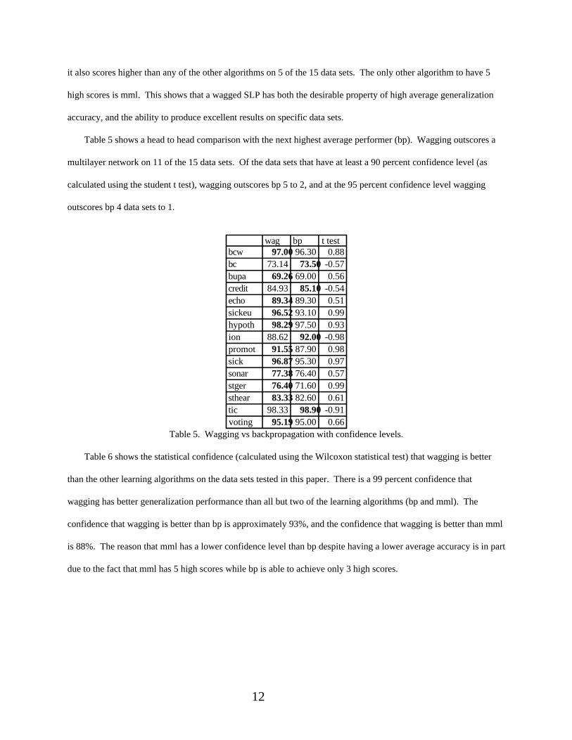
it also scores higher than any of the other algorithms on 5 of the 15 data sets. The only other algorithm to have 5

high scores is mml. This shows that a wagged SLP has both the desirable property of high average generalization

accuracy, and the ability to produce excellent results on specific data sets.

Table 5 shows a head to head comparison with the next highest average performer (bp). Wagging outscores a

multilayer network on 11 of the 15 data sets. Of the data sets that have at least a 90 percent confidence level (as

calculated using the student t test), wagging outscores bp 5 to 2, and at the 95 percent confidence level wagging

outscores bp 4 data sets to 1.

wag bp t testbcw 97.00 96.30 0.88bc 73.14 73.50 -0.57bupa 69.26 69.00 0.56credit 84.93 85.10 -0.54echo 89.34 89.30 0.51sickeu 96.52 93.10 0.99hypoth 98.29 97.50 0.93ion 88.62 92.00 -0.98promot 91.55 87.90 0.98sick 96.87 95.30 0.97sonar 77.38 76.40 0.57stger 76.40 71.60 0.99sthear 83.33 82.60 0.61tic 98.33 98.90 -0.91voting 95.19 95.00 0.66

Table 5. Wagging vs backpropagation with confidence levels.

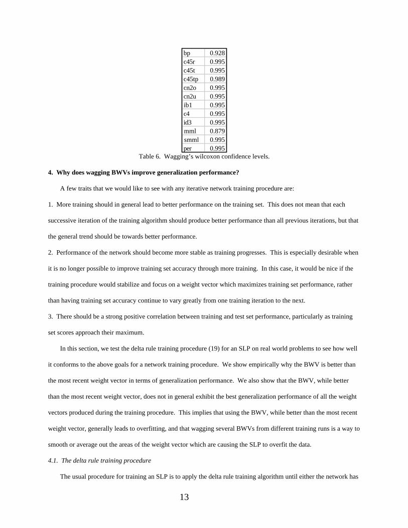
Table 6 shows the statistical confidence (calculated using the Wilcoxon statistical test) that wagging is better

than the other learning algorithms on the data sets tested in this paper. There is a 99 percent confidence that

wagging has better generalization performance than all but two of the learning algorithms (bp and mml). The

confidence that wagging is better than bp is approximately 93%, and the confidence that wagging is better than mml

is 88%. The reason that mml has a lower confidence level than bp despite having a lower average accuracy is in part

due to the fact that mml has 5 high scores while bp is able to achieve only 3 high scores.

13

bp 0.928c45r 0.995c45t 0.995c45tp 0.989cn2o 0.995cn2u 0.995ib1 0.995c4 0.995id3 0.995mml 0.879smml 0.995per 0.995

Table 6. Wagging’s wilcoxon confidence levels.

4. Why does wagging BWVs improve generalization performance?

A few traits that we would like to see with any iterative network training procedure are:

1. More training should in general lead to better performance on the training set. This does not mean that each

successive iteration of the training algorithm should produce better performance than all previous iterations, but that

the general trend should be towards better performance.

2. Performance of the network should become more stable as training progresses. This is especially desirable when

it is no longer possible to improve training set accuracy through more training. In this case, it would be nice if the

training procedure would stabilize and focus on a weight vector which maximizes training set performance, rather

than having training set accuracy continue to vary greatly from one training iteration to the next.

3. There should be a strong positive correlation between training and test set performance, particularly as training

set scores approach their maximum.

In this section, we test the delta rule training procedure (19) for an SLP on real world problems to see how well

it conforms to the above goals for a network training procedure. We show empirically why the BWV is better than

the most recent weight vector in terms of generalization performance. We also show that the BWV, while better

than the most recent weight vector, does not in general exhibit the best generalization performance of all the weight

vectors produced during the training procedure. This implies that using the BWV, while better than the most recent

weight vector, generally leads to overfitting, and that wagging several BWVs from different training runs is a way to

smooth or average out the areas of the weight vector which are causing the SLP to overfit the data.

4.1. The delta rule training procedure

The usual procedure for training an SLP is to apply the delta rule training algorithm until either the network has

14

converged to a solution or a maximum number of iterations has been reached. We say that a network has converged

to a solution when there is no longer any error on the training set, or when the total sum squared error (TSSE) on the

training set has dropped below a user defined threshold, where the total sum square error is defined as

tk − ok( )k∑ 2

(8)

Where ok is defined to be the output of the network for example k

The threshold is generally set to zero for binary output classes. Whether the training algorithm halts due to

reaching the maximum number of iterations or because the error has dropped below the threshold, the most recent

weight vector is used by the network for classification of novel examples.

There are some inherent problems with this approach, as we will show with the results later in this section.

Generally, the training instances are randomly permuted at each iteration of the delta rule algorithm.

Let

wi = weight vector produced after training iteration i

P(wi,data) = accuracy of wi on a set of data

Due to the randomness of the training procedure, and also due to the cyclical nature of the delta rule algorithm,

it is often observed that

for i > j, P(wi,train) < P(wj,train)

In other words, there is no guarantee that the current weight vector produced by the delta rule algorithm is better

(more accuracte on the training set) than some previously produced weight vector. One might hope that P(wi,train)

will be nearly as good as P(wj,train), or that as training progresses their will be a high probability that P(wi,train) will

be as good as (or nearly as good as) P(wj,train). But for most of the real world problems tested in this paper this type

of asymptotic, stable performance is not observed.

Another problem is the degree of correlation between P(wi,train) and P(wi,test). While this correlation is nearly

always positive when taken across all training iterations, the correlation can be negative if we restrict the calculation

to, say, the set of wi which corresponds to the top n training set scores. This means that choosing the single most

accurate weight vector will often not maximize test set performance.

4.2. Experiments and Results

15

All of the results in this section were obtained using the standard delta rule training algorithm. The learning rate

was set to 1, network weights were updated after the presentation of each pattern, and patterns were randomly

permuted for each iteration. Training was halted at 100,000 iterations or when the TSSE reached zero, whichever

occured first. The results reported in section 2.2.1 are from individual training runs. The results reported in section

3.2.2 are averages from 10 runs using 10-fold cross validation.

This first item we examine is the variability in training accuracy as the training procedure progresses. Even

though there is no guarantee that the most recent weight vector is the best so far, we would like to see the variability

in training set accuracy decrease, and the average training set score increase with the number of training epochs.

This would lead to a high likelihood that the most current weight vector is as accurate, or nearly as accuracte, as the

most accurate weight vector generated during training.

4.2.1 Training set performance

16

last 1000 iterations

30

40

50

60

70

80

1 101 201 301 401 501 601 701 801 901 1001

first 1000 iterations

30

40

50

60

70

80

1 101 201 301 401 501 601 701 801 901 1001

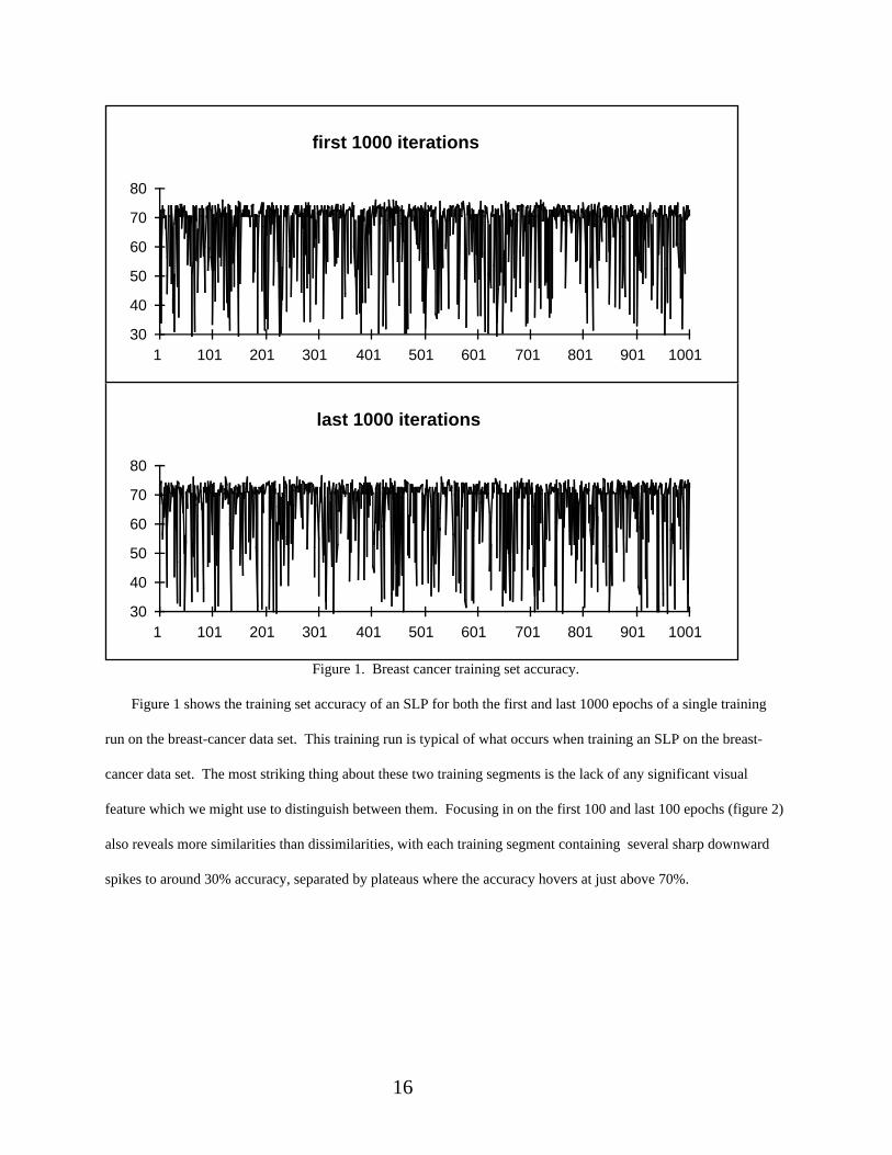
Figure 1. Breast cancer training set accuracy.

Figure 1 shows the training set accuracy of an SLP for both the first and last 1000 epochs of a single training

run on the breast-cancer data set. This training run is typical of what occurs when training an SLP on the breast-

cancer data set. The most striking thing about these two training segments is the lack of any significant visual

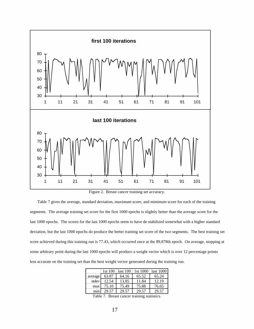
feature which we might use to distinguish between them. Focusing in on the first 100 and last 100 epochs (figure 2)

also reveals more similarities than dissimilarities, with each training segment containing several sharp downward

spikes to around 30% accuracy, separated by plateaus where the accuracy hovers at just above 70%.

17

first 100 iterations

30

40

50

60

70

80

1 11 21 31 41 51 61 71 81 91 101

last 100 iterations

30

40

50

60

70

80

1 11 21 31 41 51 61 71 81 91 101

Figure 2. Breast cancer training set accuracy.

Table 7 gives the average, standard deviation, maximum score, and minimum score for each of the training

segments. The average training set score for the first 1000 epochs is slightly better than the average score for the

last 1000 epochs. The scores for the last 1000 epochs seem to have de stabilized somewhat with a higher standard

deviation, but the last 1000 epochs do produce the better training set score of the two segments. The best training set

score achieved during this training run is 77.43, which occurred once at the 89,878th epoch. On average, stopping at

some arbitrary point during the last 1000 epochs will produce a weight vector which is over 12 percentage points

less accurate on the training set than the best weight vector generated during the training run.

1st 100 last 100 1st 1000 last 1000average 63.87 64.16 65.52 65.24

stdev 12.54 13.85 11.84 12.19max 75.10 75.49 75.88 76.65min 29.57 29.57 29.57 29.57Table 7. Breast cancer training statistics.

18

The breast cancer data set is one of the more difficult ones for an SLP to achieve high training accuracy on, with

a maximum possible training accuracy of less than 80 percent, and we would expect training set scores to show

some variability from one epoch to the next. But the degree of variability in training set scores is still surprising, and

this kind of variability is not atypical, even for data sets which are easier for the perceptron to learn.

first 100 iterations

40

60

80

100

1 21 41 61 81 101

last 100 iterations

40

60

80

100

1 21 41 61 81 101

first 1000 iterations

40

60

80

100

1 251 501 751 1001

last 1000 iterations

40

60

80

100

1 251 501 751 1001

Figure 3. Echocardiogram training set accuracy.

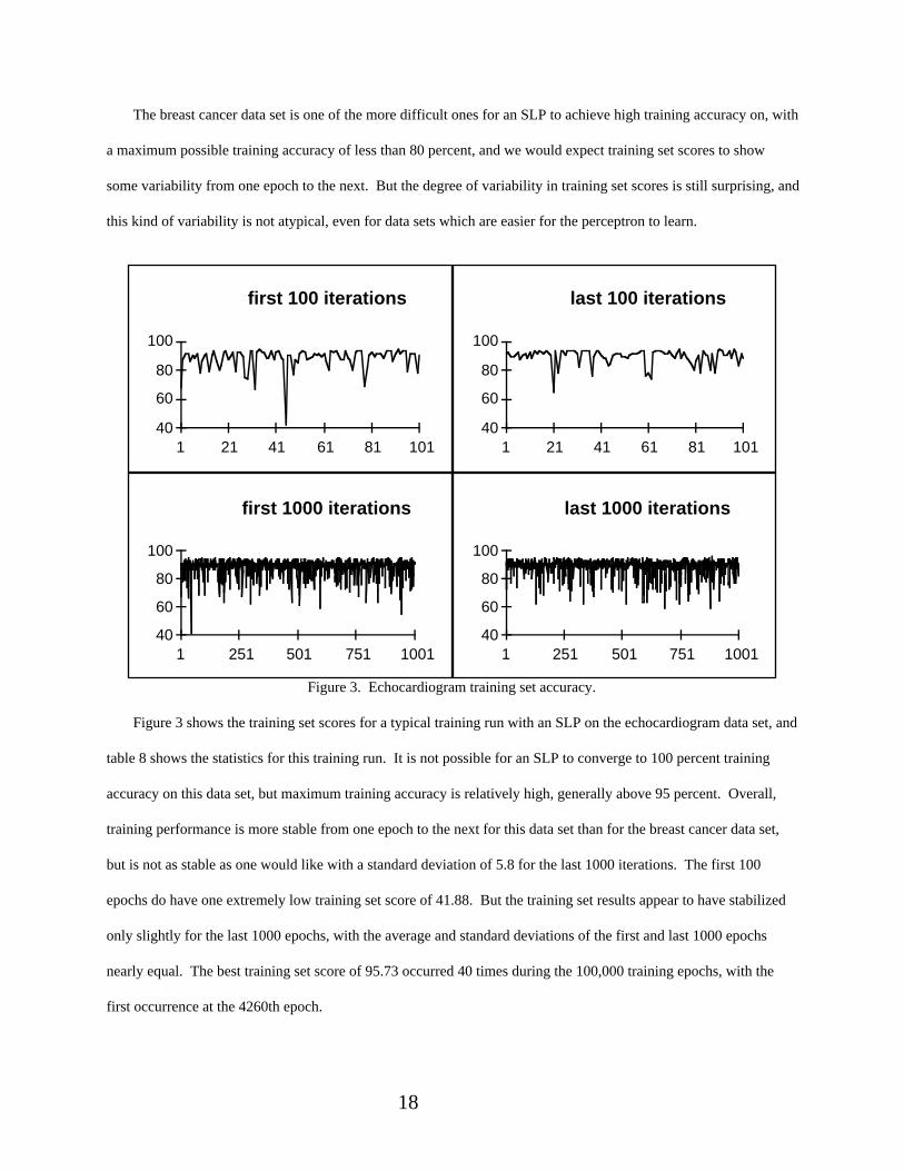
Figure 3 shows the training set scores for a typical training run with an SLP on the echocardiogram data set, and

table 8 shows the statistics for this training run. It is not possible for an SLP to converge to 100 percent training

accuracy on this data set, but maximum training accuracy is relatively high, generally above 95 percent. Overall,

training performance is more stable from one epoch to the next for this data set than for the breast cancer data set,

but is not as stable as one would like with a standard deviation of 5.8 for the last 1000 iterations. The first 100

epochs do have one extremely low training set score of 41.88. But the training set results appear to have stabilized

only slightly for the last 1000 epochs, with the average and standard deviations of the first and last 1000 epochs

nearly equal. The best training set score of 95.73 occurred 40 times during the 100,000 training epochs, with the

first occurrence at the 4260th epoch.

19

1st 100 last 100 1st 1000 last 1000average 88.18 89.69 88.89 89.21

stdev 7.50 5.28 6.04 5.79max 94.87 94.87 94.87 95.73min 41.88 64.96 41.88 58.97

Table 8. Echocardiogram training statistics.

1st 100 iterations

40

60

80

100

1 21 41 61 81 101

last 100 iterations

40

60

80

100

1 21 41 61 81 101

last 1000 iterations

40

60

80

100

1 251 501 751 1001

1st 1000 iterations

40

60

80

100

1 251 501 751 1001

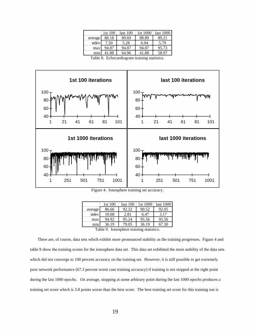
Figure 4. Ionosphere training set accuracy.

1st 100 last 100 1st 1000 last 1000average 86.66 92.32 90.52 92.05

stdev 10.68 2.81 6.47 3.17max 94.92 95.24 95.56 95.56min 36.19 79.05 36.19 67.30

Table 9. Ionosphere training statistics.

There are, of course, data sets which exhibit more pronounced stability as the training progresses. Figure 4 and

table 9 show the training scores for the ionosphere data set. This data set exhibited the most stability of the data sets

which did not converge to 100 percent accuracy on the training set. However, it is still possible to get extremely

poor network performance (67.3 percent worst case training accuracy) if training is not stopped at the right point

during the last 1000 epochs. On average, stopping at some arbitrary point during the last 1000 epochs produces a

training set score which is 3.8 points worse than the best score. The best training set score for this training run is

20

95.87, which occurred at the 9623rd epoch. This score was repeated 3 times during the 100,000 training epochs.

first 100 iterations

50

75

100

1 21 41 61 81 101

last 100 iterations

50

75

100

1 21 41 61 81 101

last 1000 iterations

50

75

100

1 251 501 751 1001

first 1000 iterations

50

75

100

1 251 501 751 1001

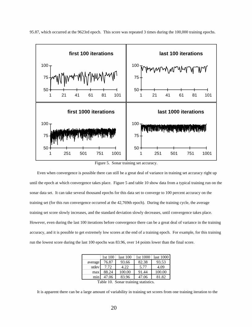
Figure 5. Sonar training set accuracy.

Even when convergence is possible there can still be a great deal of variance in training set accuracy right up

until the epoch at which convergence takes place. Figure 5 and table 10 show data from a typical training run on the

sonar data set. It can take several thousand epochs for this data set to converge to 100 percent accuracy on the

training set (for this run convergence occurred at the 42,769th epoch). During the training cycle, the average

training set score slowly increases, and the standard deviation slowly decreases, until convergence takes place.

However, even during the last 100 iterations before convergence there can be a great deal of variance in the training

accuracy, and it is possible to get extremely low scores at the end of a training epoch. For example, for this training

run the lowest score during the last 100 epochs was 83.96, over 14 points lower than the final score.

1st 100 last 100 1st 1000 last 1000average 76.87 93.66 82.38 93.53

stdev 7.72 4.22 5.77 4.09max 88.24 100.00 91.44 100.00min 47.06 83.96 47.06 81.82

Table 10. Sonar training statistics.

It is apparent there can be a large amount of variability in training set scores from one training iteration to the

21

next with the 4 example data sets shown in this section. The variability of training set scores exhibited by these data

sets is typical for the real world data sets tested in this paper. Assuming that these results hold for general real world

problems, this means that using the most recent weight vector (after stopping at a maximum iteration count) will

generally lead to a network with subpar performance in terms of training set accuracy. The goal, however, is to

produce a network with high test set accuracy, which will not necessarily be the network with the highest training set

accuracy. We examine this issue in the next section.

4.2.2 The correlation between training and test set accuracy

It is relatively simple to solve the problem of variable end-of-epoch training set scores by testing the network at

the end of each epoch and saving the weight settings which produce the highest accuracy on the training set. This

can continue as long as the best weight vector is improving or until some set number of iterations has been reached.

The penalty that is incurred by this procedure is an approximate two-fold increase in computational complexity.

Instead of one pass through the training set, two passes through the training set are required for each training

iteration. The first pass adjusts the weight vector, and the second pass determines the accuracy of the new weight

vector on the training set.

One would save the best weight vector on the assumption that high training accuracy correlates well with high

test set accuracy. We show that while this assumption is not reasonable, it is still better to use the weight vector

which produced the highest training set accuracy during the training phase than it is to use the most recent weight

vector produced at the end of the training phase.

We use Pearsons correlation, which measures the degree of correlation between two variables, to calculate the

correlation between the training and test set scores. The formula for calculating Pearson’s correlation is

r =XY −

X Y∑∑N

∑

X2 −X∑( )2

N∑

⎛

⎝⎜⎜

⎞

⎠⎟⎟

Y 2 −Y∑( )2

N∑

⎛

⎝⎜⎜

⎞

⎠⎟⎟

(1)

Where N = the number of samplesX, Y = the paired values

With this measure, a 1 indicates a complete positive linear correlation of training and test set scores, a 0

indicates no correlation, and a -1 indicates a perfect negative linear correlation.

22

Table 11 shows the correlation, calculated with Pearson’s formula, of training and test set scores for the 15 data

sets tested in this paper. These scores are calculated from statistics gathered during 10 training runs using 10 fold

cross validation on the original data sets. The maximum number of iterations was set at 100,000.

bc 0.86bcw 0.77bupa 0.73credit 0.83echo 0.48hypo 0.93ion 0.48promo 0.77sick 0.96euth 0.93sonar 0.18stger 0.90sthear 0.67tic 0.46vote -0.40average 0.64

Table 11. Correlation between training and test set scores.

While most of the data sets have a high positive correlation between the training and test set accuracies at the

end of each epoch, there are a few data sets which have a weak correlation. Ironically, the voting data set is the only

data set which has a negative correlation between the training and test set scores generated by the delta rule training

algorithm (some would say that this counter intuitive result is an indication that voting in the House of

Representatives is as illogical as everyone suspects it to be). We will discuss why this data set exhibits a negative

correlation shortly.

The fact that all of the data sets (with one exception) exhibited a positive correlation between their training and

test set scores does not imply that there is a tendency for test set scores to continue to increase as the training set

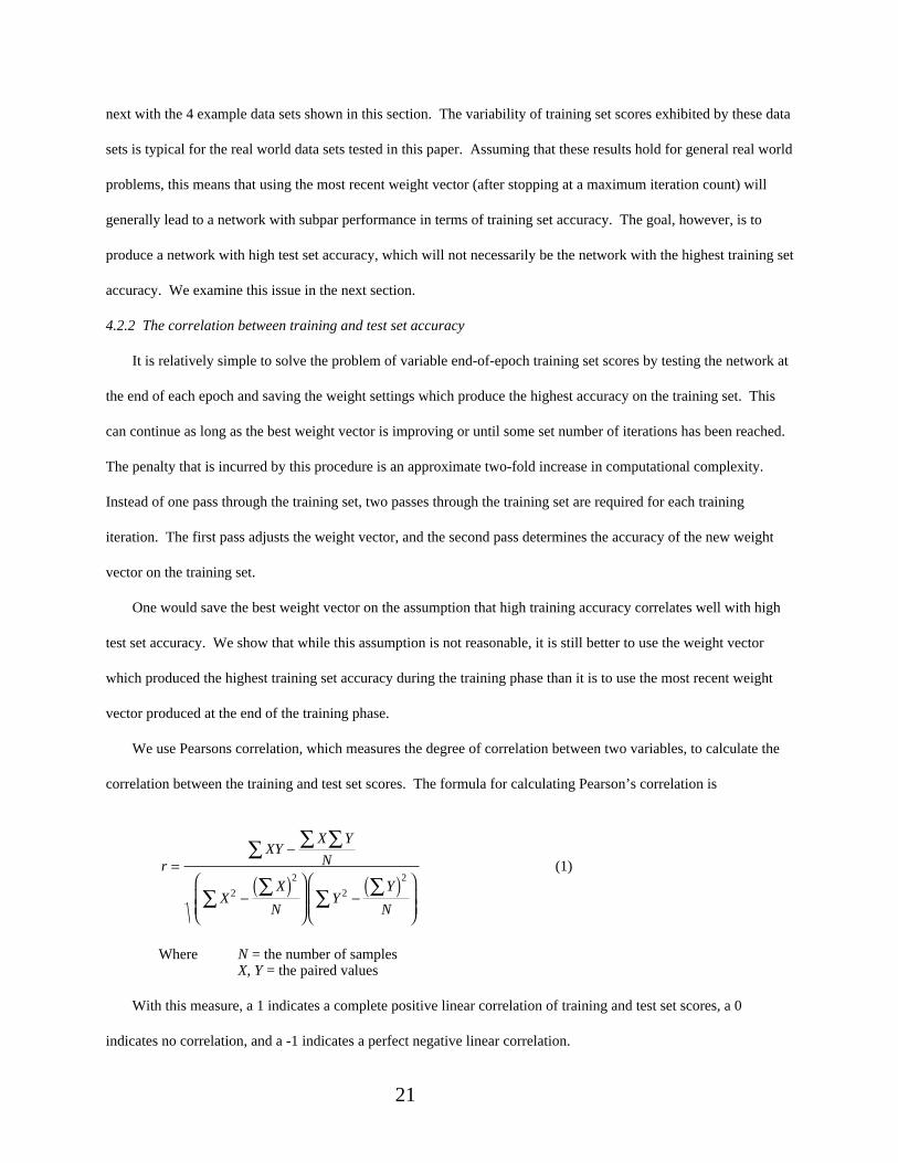
score nears its maximum. Figure 6 shows the average performance (top 20 training scores and associated average

test set scores) for all of the data sets except the voting data set. Even for these data sets, which all exhibited a

positive training-test correlation, the test accuracy peaks (on average) at the 4th highest training set score, and

thereafter decreases. So most of the data sets would exhibit a negative correlation if the calculation was restricted to

use only the top 3 or 4 training set scores and associated test set scores. Of the 15 data sets, only 4 of the sets had an

average test set accuracy which peaked at the highest training set score. What this means is that, at least with the

data sets tested in this paper, selecting the most accurate weight vector for the SLP will in general lead to overfitting.

23

83

85

87

89

91

5 10 15 20

train

test

Figure 6. Averages over all the data sets of the top 20 training set scores.

82

87

92

97

train

test

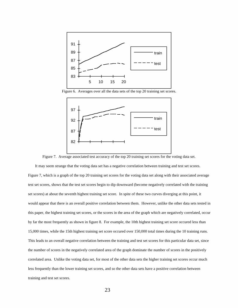
Figure 7. Average associated test accuracy of the top 20 training set scores for the voting data set.

It may seem strange that the voting data set has a negative correlation between training and test set scores.

Figure 7, which is a graph of the top 20 training set scores for the voting data set along with their associated average

test set scores, shows that the test set scores begin to dip downward (become negatively correlated with the training

set scores) at about the seventh highest training set score. In spite of these two curves diverging at this point, it

would appear that there is an overall positive correlation between them. However, unlike the other data sets tested in

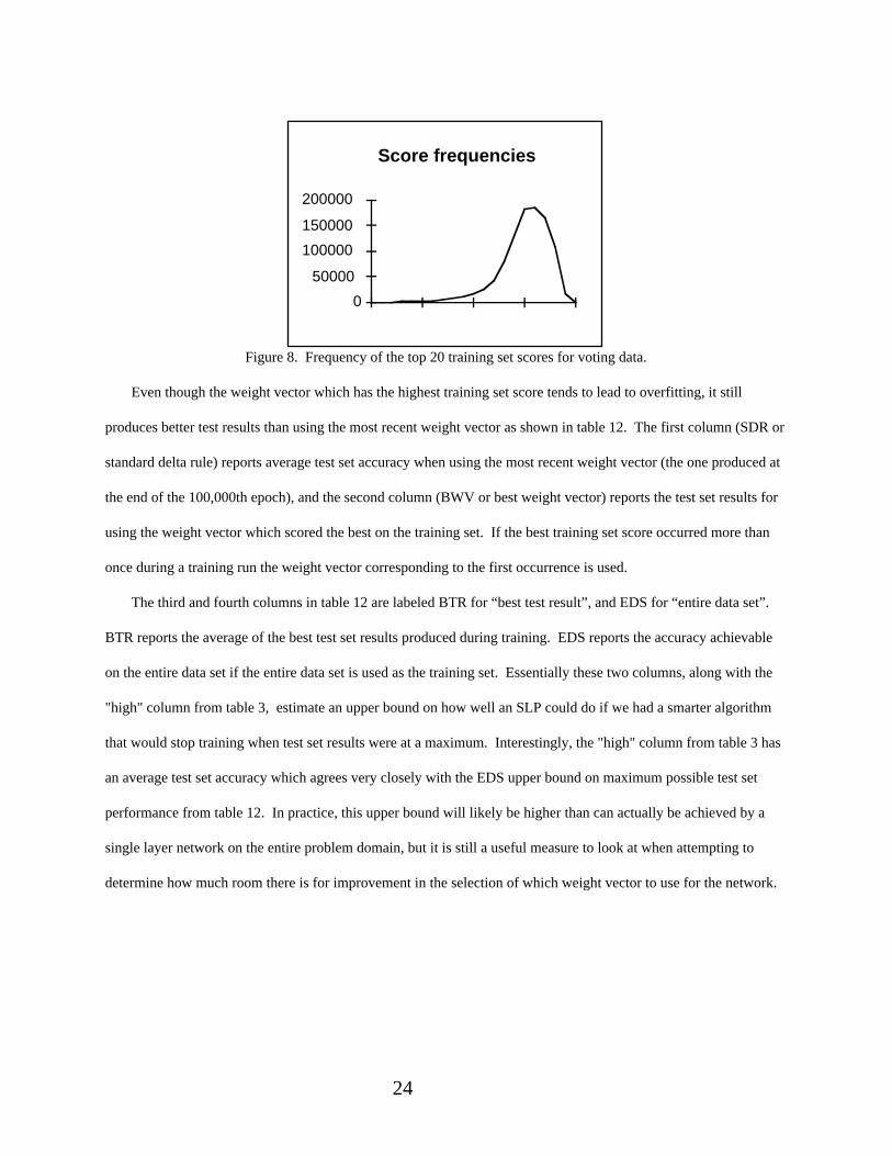
this paper, the highest training set scores, or the scores in the area of the graph which are negatively correlated, occur

by far the most frequently as shown in figure 8. For example, the 10th highest training set score occured less than

15,000 times, while the 15th highest training set score occured over 150,000 total times during the 10 training runs.

This leads to an overall negative correlation between the training and test set scores for this particular data set, since

the number of scores in the negatively correlated area of the graph dominate the number of scores in the positively

correlated area. Unlike the voting data set, for most of the other data sets the higher training set scores occur much

less frequently than the lower training set scores, and so the other data sets have a positive correlation between

training and test set scores.

24

Score frequencies

0

50000

100000

150000

200000

Figure 8. Frequency of the top 20 training set scores for voting data.

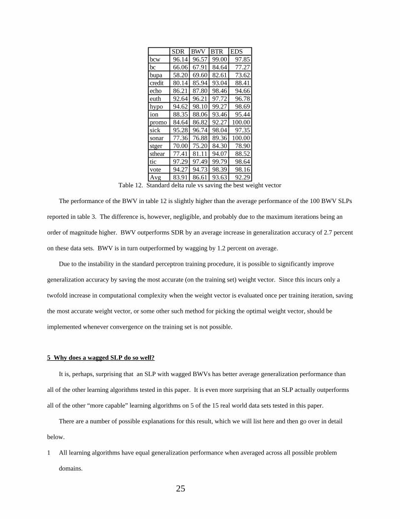
Even though the weight vector which has the highest training set score tends to lead to overfitting, it still

produces better test results than using the most recent weight vector as shown in table 12. The first column (SDR or

standard delta rule) reports average test set accuracy when using the most recent weight vector (the one produced at

the end of the 100,000th epoch), and the second column (BWV or best weight vector) reports the test set results for

using the weight vector which scored the best on the training set. If the best training set score occurred more than

once during a training run the weight vector corresponding to the first occurrence is used.

The third and fourth columns in table 12 are labeled BTR for “best test result”, and EDS for “entire data set”.

BTR reports the average of the best test set results produced during training. EDS reports the accuracy achievable

on the entire data set if the entire data set is used as the training set. Essentially these two columns, along with the

"high" column from table 3, estimate an upper bound on how well an SLP could do if we had a smarter algorithm

that would stop training when test set results were at a maximum. Interestingly, the "high" column from table 3 has

an average test set accuracy which agrees very closely with the EDS upper bound on maximum possible test set

performance from table 12. In practice, this upper bound will likely be higher than can actually be achieved by a

single layer network on the entire problem domain, but it is still a useful measure to look at when attempting to

determine how much room there is for improvement in the selection of which weight vector to use for the network.

25

SDR BWV BTR EDSbcw 96.14 96.57 99.00 97.85bc 66.06 67.91 84.64 77.27bupa 58.20 69.60 82.61 73.62credit 80.14 85.94 93.04 88.41echo 86.21 87.80 98.46 94.66euth 92.64 96.21 97.72 96.78hypo 94.62 98.10 99.27 98.69ion 88.35 88.06 93.46 95.44promo 84.64 86.82 92.27 100.00sick 95.28 96.74 98.04 97.35sonar 77.36 76.88 89.36 100.00stger 70.00 75.20 84.30 78.90sthear 77.41 81.11 94.07 88.52tic 97.29 97.49 99.79 98.64vote 94.27 94.73 98.39 98.16Avg 83.91 86.61 93.63 92.29

Table 12. Standard delta rule vs saving the best weight vector

The performance of the BWV in table 12 is slightly higher than the average performance of the 100 BWV SLPs

reported in table 3. The difference is, however, negligible, and probably due to the maximum iterations being an

order of magnitude higher. BWV outperforms SDR by an average increase in generalization accuracy of 2.7 percent

on these data sets. BWV is in turn outperformed by wagging by 1.2 percent on average.

Due to the instability in the standard perceptron training procedure, it is possible to significantly improve

generalization accuracy by saving the most accurate (on the training set) weight vector. Since this incurs only a

twofold increase in computational complexity when the weight vector is evaluated once per training iteration, saving

the most accurate weight vector, or some other such method for picking the optimal weight vector, should be

implemented whenever convergence on the training set is not possible.

5 Why does a wagged SLP do so well?

It is, perhaps, surprising that an SLP with wagged BWVs has better average generalization performance than

all of the other learning algorithms tested in this paper. It is even more surprising that an SLP actually outperforms

all of the other “more capable” learning algorithms on 5 of the 15 real world data sets tested in this paper.

There are a number of possible explanations for this result, which we will list here and then go over in detail

below.

1 All learning algorithms have equal generalization performance when averaged across all possible problem

domains.

26

2 There are no (or very few) high order correlations in the data.

3 The high order correlations in the data are difficult to find.

4 Wagging removes overfitting through averaging.

1. There is some indication that it is difficult for a single learning algorithm to outperform all other learning

algorithms on a large variety of problems [27, 33]. While there have been some interesting theoretical results

developed in an attempt to make it possible to prove that one learning algorithm is better than another [30, 4, 31, 32,

], all of these results are based on determining the probability of error given the data and the function from which

the data are drawn, or P(E|d,f). However, learning algorithms are usually only presented with the data, so for the

general real world case we are concerned only with P(E|d). But if all we are given is the data, then it is impossible to

prove that one learning algorithm is better than another. In fact it is worse than this, since it is possible to prove that

if all we are given is the data (observations) then no machine learning algorithm will outperform any other

algorithm. In other words, the sum total generalization performance of all learning algorithms is equal and no better

than random across all problem domains.

For the most part we are interested in real world problems, not in all problem domains, and so it may be that

some learning algorithm will outperform all others for the real world problems. Still, there are a large variety of

problems that fall under this categorization, and the more problems that one tests on, the more likely it is that a more

complex learning algorithm will have a difficult time beating the average performance of a simple learning

algorithm, or visa versa. The fact that the SLP outperforms the other algorithms may only mean that the data sets

tested in this paper are well suited to the SLP, and that there are other real world problems which the SLP will

perform poorly on.

2. Whether or not one algorithm will be able to perform better than all others on real world problems depends

on what types of characteristics real world problems have, their tendencies and so forth. It is possible that the better

performance of an SLP on the problems tested in this paper is due to none of the data sets having any high order

correlations between inputs and output classification. Evidence of this lack of higher order correlations in real world

data sets can be seen in the relatively good performance of the extremely simple 1-rules learning algorithm ([14]),

and in the performance of the wagged SLP. When choosing features to use with a real world classification problem,

people tend to choose features which they feel are correlated with the output data. More often than not, the features

27

that people choose will be those which exhibit first order correlations with the output classification, and potentially

little if any higher order correlation's. Otherwise, had the person designing the data set known of some higher order

correlation in the data, they probably would have incorporated it into the data set as a single input feature.

Learning algorithms that look for, or are capable of handling higher order correlations will tend not to perform

as well on data sets which have no such correlations, since any higher order correlations that they ‘find’ will not be

valid. This problem is exacerbated if the first order correlations which the features exhibit are not sufficient to

correctly classify all of the examples in the training set. In this case, learning algorithms such as bp will be pushed

to find higher order correlations (which do not really exist) in order to correctly classify all training examples. We

refer to this problem as overfitting. It is also often referred to as over learning or memorization of the training set.

Any higher order correlations which are found in such case are invalid, and will hurt generalization performance.

3. Even when there are higher order correlations in the data this does not mean that an algorithm which can find

such correlations will do any better than one which cannot. The problem is that the learning algorithm must find the

right higher order correlations, or nearly the right ones, and not just ones that match the training data in order for

them to be of benefit, and it may have to do so without enough data to properly constrain the hypothesis search

space for the learning algorithm. The learning algorithm that one chooses will bias the type of higher order

correlations which are most likely to be discovered, and the correlations it tends to discover may or may not be

appropriate for particular problem domains. When they are not appropriate (do not fit naturally with the actual

higher order correlation from the problem domain) generalization performance will suffer.

For example, a higher order network (HON) is a network which uses multiplication (usually, but can use any

nonlinear function) to combine original input features into higher order features. If the right set of higher order

features are chosen a HON is theoretically capable of correctly classifying any consistent training set. In fact, there

is a polynomial algorithm which, given any data set, will choose just such a feature set for a HON (22). However,

while the higher order features may be ‘right’ for the training set, there is no guarantee that they will closely match

the higher order correlations that exist in the problem domain. The probability that the HON features will match the

actual higher order features (and thus lead to better generalization performance) will in part be related to the size of

the training set, the search algorithm, how many higher order correlations there are, and how well multiplication

matches the true nonlinear, higher order correlations from the problem domain. For many real world data sets this

28

probability can be vanishingly small, and depending upon how small it is, one may be better off sticking with a

learning algorithm that ignores the possibility of such higher order correlations.

4. In the case where there are no high order correlations in the data, or when the high order correlations are

unlikely to be identified by a more complex learning algorithm, it makes sense to use a learning algorithm which

ignores such possibilities, such as an SLP. Wagging several SLPs averages out any overfitting that may occur in a

single training run, and thus can produce an SLP with better average generalization performance than a single un-

wagged SLP.

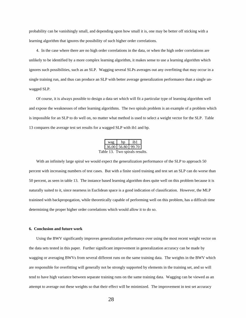
Of course, it is always possible to design a data set which will fit a particular type of learning algorithm well

and expose the weaknesses of other learning algorithms. The two spirals problem is an example of a problem which

is impossible for an SLP to do well on, no matter what method is used to select a weight vector for the SLP. Table

13 compares the average test set results for a wagged SLP with ib1 and bp.

wag bp ib136.00 56.80 99.70

Table 13. Two spirals results.

With an infinitely large spiral we would expect the generalization performance of the SLP to approach 50

percent with increasing numbers of test cases. But with a finite sized training and test set an SLP can do worse than

50 percent, as seen in table 13. The instance based learning algorithm does quite well on this problem because it is

naturally suited to it, since nearness in Euclidean space is a good indication of classification. However, the MLP

trainined with backpropogation, while theoretically capable of performing well on this problem, has a difficult time

determining the proper higher order correlations which would allow it to do so.

6. Conclusion and future work

Using the BWV significantly improves generalization performance over using the most recent weight vector on

the data sets tested in this paper. Further significant improvement in generalization accuracy can be made by

wagging or averaging BWVs from several different runs on the same training data. The weights in the BWV which

are responsible for overfitting will generally not be strongly supported by elements in the training set, and so will

tend to have high variance between separate training runs on the same training data. Wagging can be viewed as an

attempt to average out these weights so that their effect will be minimized. The improvement in test set accuracy

29

that wagging makes on the data sets used in this paper is slightly better than that gained from bagging, with the

advantage over bagging that only a single weight vector need be stored. In addition, wagging produced test set

scores which are on average better than any of the other learning algorithms compared in this paper.

6.1 Future work

It should be possible to further improve the generalization results for an SLP. We did not implement any

procedure (other than limiting the maximum number of training iterations) to keep weight magnitudes relatively

equal across separate training runs. When averaging weights, if one of the SLPs has extremely large weights in

comparison with the other SLPs then it will tend to dominate the average. By not implementing a procedure to keep

weight magnitudes in line, this could lead to a situation where the average weights perform no differently than the

SLP that has the largest weights. So, it may be possible to improve the generalization results of the wagged SLP

even further by normalizing the weight vectors before averaging them, or perhaps by using some form of weight

decay to keep weights from having overly large magnitude.

Another area where improvements can be made is in the training procedure itself. A more stable, asymptotic

training method might lead to better weight vector estimates and thus a better average weight vector. We have done

some experiments where we have tried to smooth the transition from one weight vector to the next during training by

using a local windowed averaging scheme. By combining this smoothing technique with a momentum term we have

been able to improve convergence times by an order of magnitude on the sonar data set (from over 40,000 iterations

down to about 2,000).

Currently we are focusing our research on using wagging with multi-layer networks. Work which has already

been done on this prebiases the weight vector to be in a certain area of the weight space through an initial training

run that uses all of the available training data, and then creates multiple copies of this weight vector and continues

training each on a different portion of the training data [29]. By so doing, the corresponding weights from different

copies of the network will be slightly different but still tend to perform the same function, and it therefore makes

sense to average them. This technique leads to improved generalization performance, at least on the few data sets

tested.

One of the drawbacks of this approach is that the weights are prebiased to be in a single area of the weight space

based only upon a single training run using a single network. It could be advantageous to explore more areas of the

30

weight space by training multiple independent network copies. Another drawback is that the multiple network

copies are only trained on a portion of the available training data. We will focus on strategies which always use all

of the available data and explore a larger area in weight space, and then slowly force or urge weights to functionally

correspond across multiple network copies, and finally average these weights to obtain a single averaged network.

We will also look at constraining the network architecture so that weights are guaranteed to functionally correspond

across different networks and training runs. We expect that in general a wagged network will exhibit better

generalization performance than a non-wagged network.