e xcited-state quantum phase transitions in systems with few degrees of freedom
DESCRIPTION
E XCITED-STATE QUANTUM PHASE TRANSITIONS IN SYSTEMS WITH FEW DEGREES OF FREEDOM. Pavel Str ánský. www.pavelstransky.cz. Institut o de Ciencias Nucleares , Universidad Nacional Aut ó noma de M éxico. In collaboration with: Pavel Cejnar. - PowerPoint PPT PresentationTRANSCRIPT
EXCITED-STATE QUANTUM PHASE TRANSITIONS IN SYSTEMS WITH FEW
DEGREES OF FREEDOM
Pavel Stránský
Seminario Lunch Nuclear, Instituto de Física, UNAM 4th October 2013
Institute of Particle and Nuclear Phycics, Faculty of Mathematics and Physics, Charles University in Prague, Czech Republic
Instituto de Ciencias Nucleares, Universidad Nacional Autónoma de México
In collaboration with: Pavel Cejnar
www.pavelstransky.cz
Michal Macek, Amiram LeviatanRacah Institute of Physics, The Hebrew University, Jerusalem, Israel
1. Excited-state quantum phase transition
2. Models- CUSP potential (1 degree of freedom)- Creagh-Whelan potential (2 degrees of freedom)
3. Signatures of the ESQPT- level density and its derivatives- thermodynamical properties- flow rate
1. Excited-State Quantum Phase Transitions
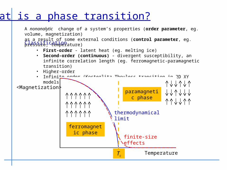
What is a phase transition?A nonanalytic change of a system’s properties (order parameter, eg. volume, magnetization)as a result of some external conditions (control parameter, eg. pressure, temperature)
• First-order - latent heat (eg. melting ice)• Second-order (continuous) - divergent susceptibility, an infinite
correlation length (eg. ferromagnetic-paramagnetic transition)• Higher-order• Infinite-order (Kosterlitz-Thouless transition in 2D XY models)
Classification
<Magnetization>
Temperature
ferromagnetic phase
paramagnetic phase
finite-size effects
thermodynamical limit
Tc
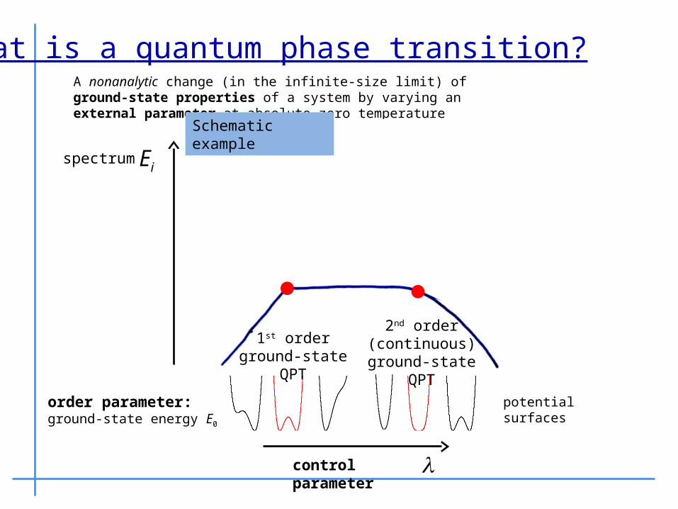
What is a quantum phase transition?A nonanalytic change (in the infinite-size limit) of ground-state properties of a system by varying an external parameter at absolute zero temperature
Ei
1st orderground-state
QPT
2nd order (continuous)ground-state
QPT
Schematic example
spectrum
control parameter
potential surfacesorder parameter: ground-state energy E0
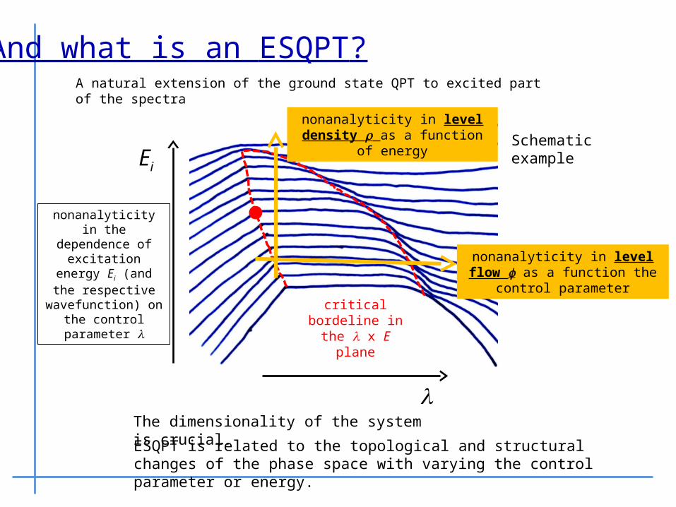
And what is an ESQPT?
Ei
nonanalyticity in the dependence of excitation energy
Ei (and the respective
wavefunction) on the control
parameter
Schematic example
nonanalyticity in level density as a function of
energy
nonanalyticity in level flow as a function the control
parameter
A natural extension of the ground state QPT to excited part of the spectra
ESQPT is related to the topological and structural changes of the phase space with varying the control parameter or energy.
The dimensionality of the system is crucial.
critical bordeline in the
x E plane
Finite models- size of the system
- number of independent components of the system
- number of degrees of freedom
Nonanalyticities in phase transitions occur only when the system’s size grows to infinity.
Finite model:
while f is maintained finite
Example: Interacting Boson Model
Generally, the number of degrees of freedom f grows with N. However, f is maintained in collective models described by some dynamical algebra A of rank r, for which
• f is related with the rank r (in s & x boson models f = r - 1)• is usually related with the considered irreducible representation of the
algebra
- b bosons (of the type s or d) – quasiparticles, generating a U(6) algebra (f = 5)- 3 degrees of freedom are always separated (conserving angular momentum)- (index of the representation of the U(6) algebra)
In quantized classical systems,
- this limit coincides with the classical limit
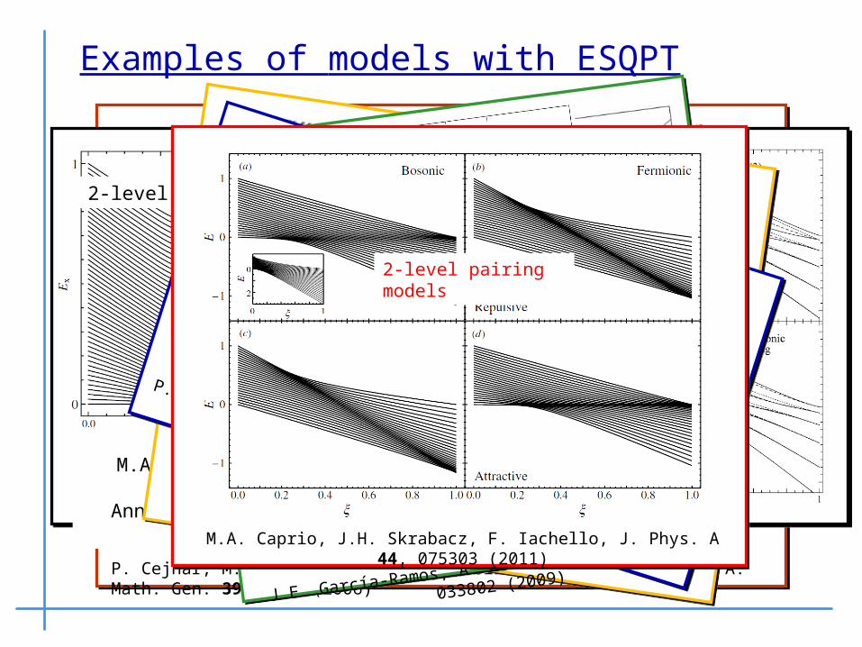
Examples of models with ESQPT
P. Cejnar, M. Macek, S. Heinze, J. Jolie, J. Dobeš, J. Phys. A: Math. Gen. 39, L515 (2006)
O(6)-U(5) transition in the Interacting Boson Model
M.A. Caprio, P. Cejnar, F. Iachello, Annals of Physics 323, 1106 (2008)
2-level fermionic pairing model
P. Cejnar, P. Stránský, Phys. Rev. E 78, 031130 (2008)
Geometric collective model of atomic nucleiLipkin model
P. Pérez-Fernández, A. Relaño, J.M. Arias, J. Dukelsky, J.E. García-
Ramos, Phys. Rev. A 80, 032111 (2009)P. Pérez-Fernández, P. Cejnar, J.M. Arias, J. Dukelsky,
J.E. García-Ramos, A. Relaño, Phys. Rev. A 83, 033802
(2009)M.A. Caprio, J.H. Skrabacz, F. Iachello, J. Phys. A 44, 075303
(2011)
2-level pairing models
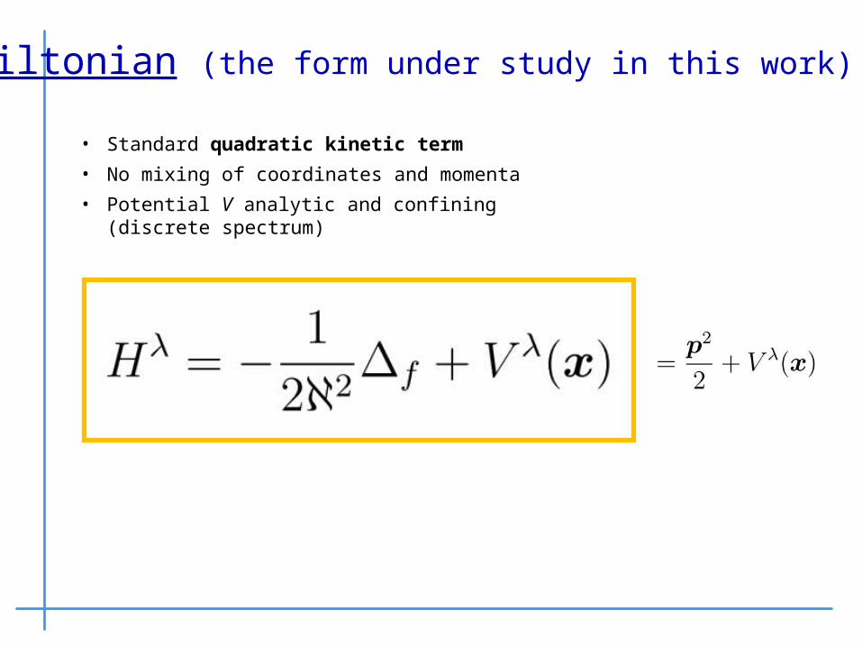
Hamiltonian (the form under study in this work)
• Standard quadratic kinetic term
• No mixing of coordinates and momenta
• Potential V analytic and confining (discrete spectrum)
2. Models
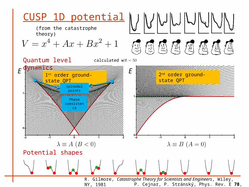
CUSP 1D potential
R. Gilmore, Catastrophe Theory for Scientists and Engineers, Wiley, NY, 1981
Quantum level dynamics
E
Potential shapes
1st order ground-state QPT
2nd order ground-state QPT
Phase coexistenc
e
spinodal points
calculated with
E
(from the catastrophe theory)
P. Cejnar, P. Stránský, Phys. Rev. E 78, 031130 (2008)
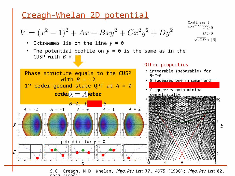
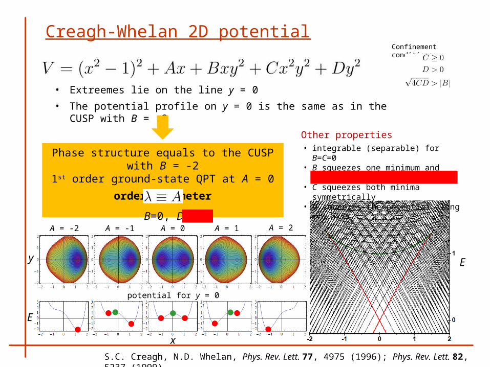
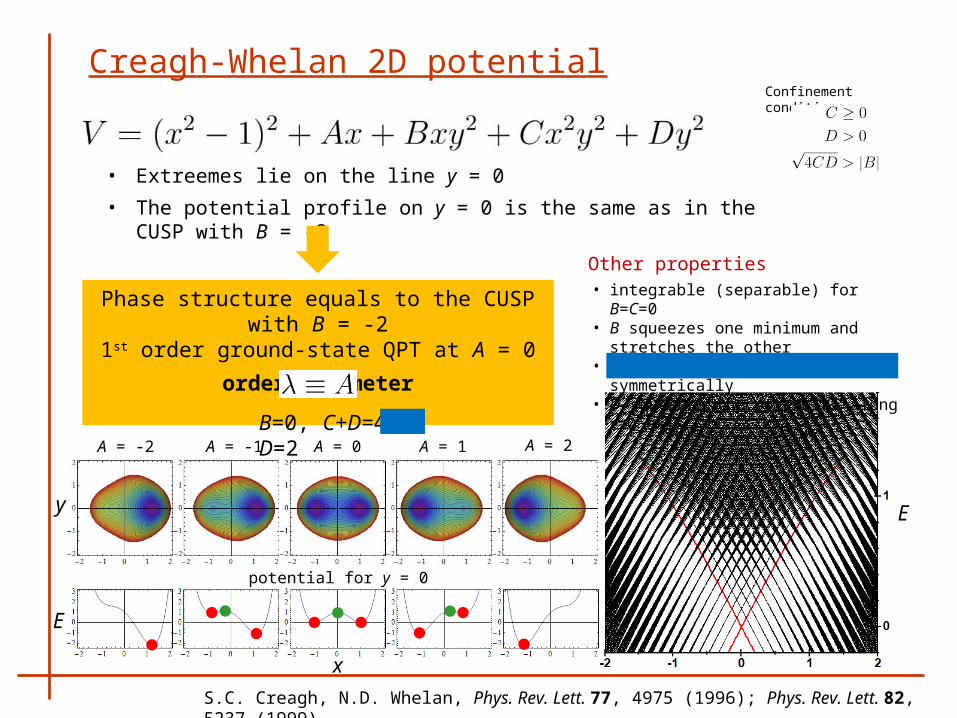
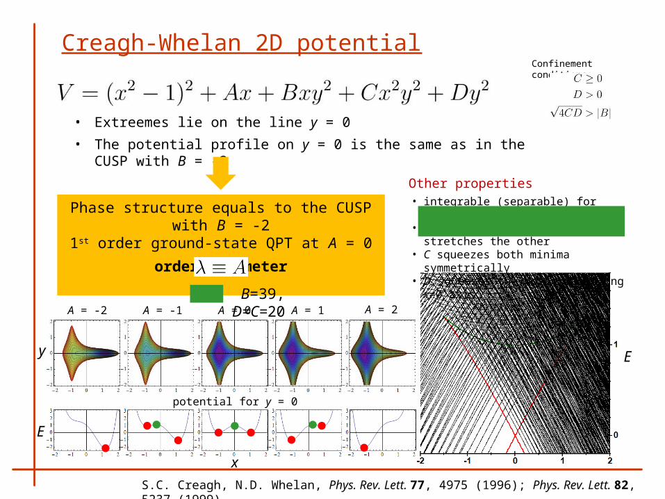
Creagh-Whelan 2D potential
S.C. Creagh, N.D. Whelan, Phys. Rev. Lett. 77, 4975 (1996); Phys. Rev. Lett. 82, 5237 (1999)
• Extreemes lie on the line y = 0
• The potential profile on y = 0 is the same as in the CUSP with B = -2
Confinement conditions:
Phase structure equals to the CUSP with B = -2
1st order ground-state QPT at A = 0
order parameter
• integrable (separable) for B=C=0• B squeezes one minimum and
stretches the other• C squeezes both minima
symmetrically• D squeezes the potential along x=0
axis
Other properties
x
y
potential for y = 0
A = -2 A = -1 A = 0 A = 1 A = 2
E
E
B=0, D=C=0.5
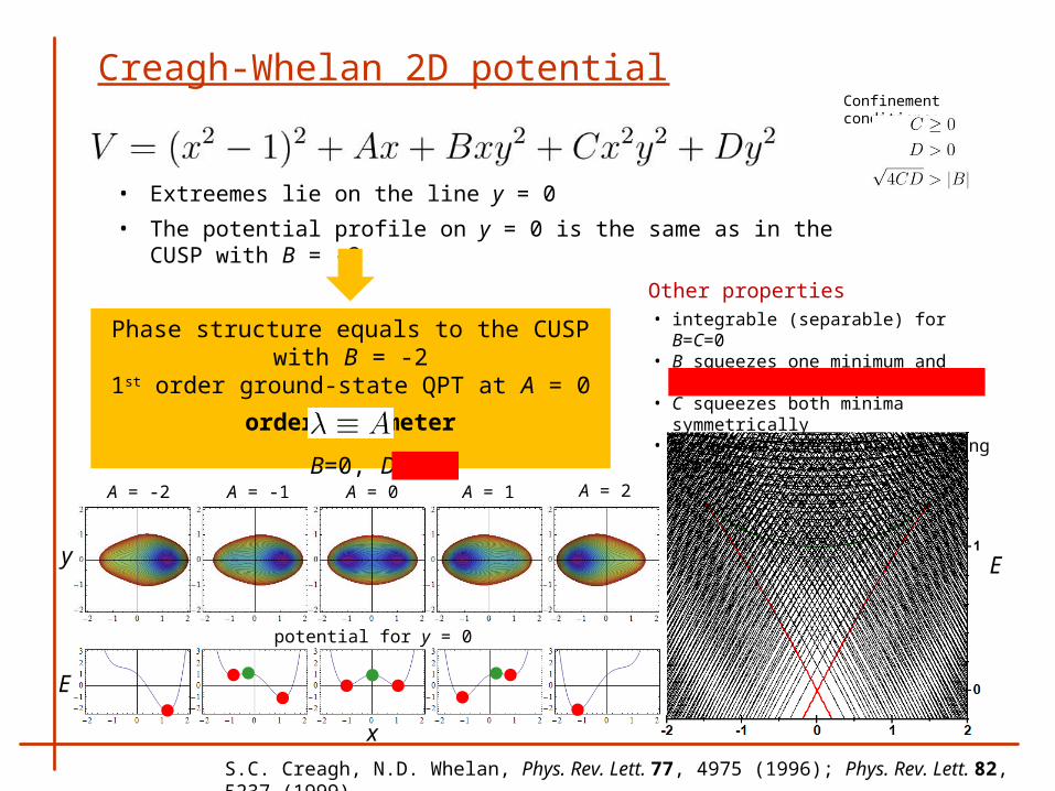
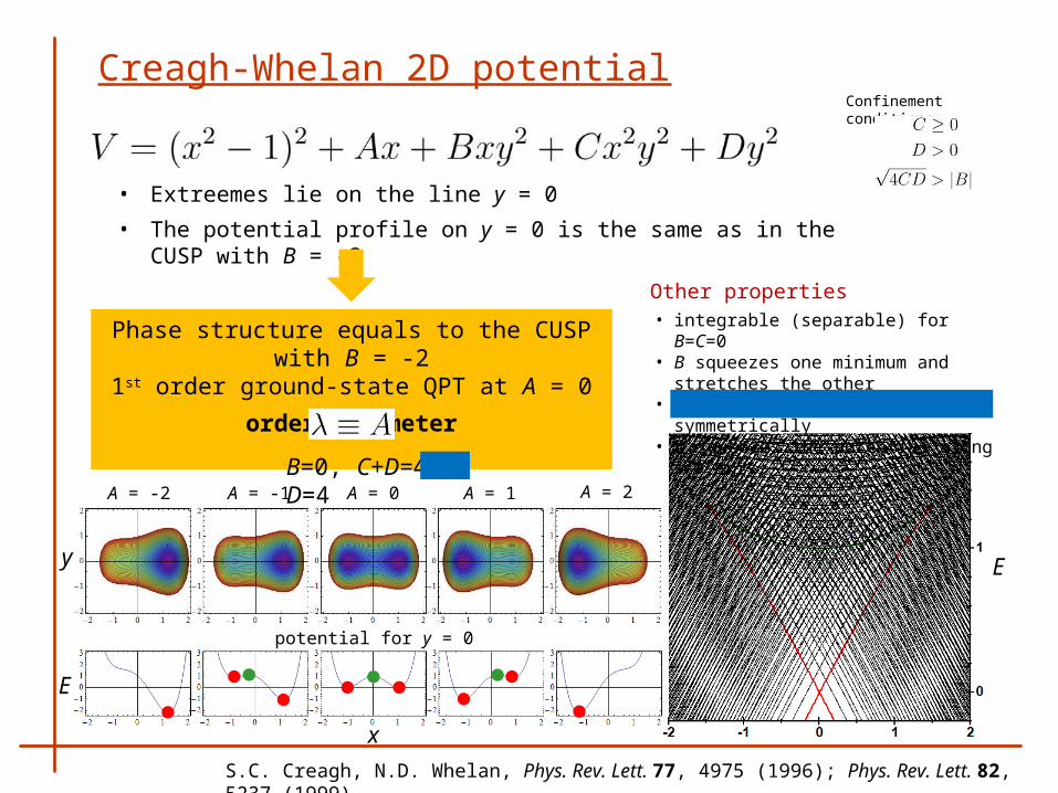
Creagh-Whelan 2D potential
S.C. Creagh, N.D. Whelan, Phys. Rev. Lett. 77, 4975 (1996); Phys. Rev. Lett. 82, 5237 (1999)
• Extreemes lie on the line y = 0
• The potential profile on y = 0 is the same as in the CUSP with B = -2
Confinement conditions:
Phase structure equals to the CUSP with B = -2
1st order ground-state QPT at A = 0
order parameter
• integrable (separable) for B=C=0• B squeezes one minimum and
stretches the other• C squeezes both minima
symmetrically• D squeezes the potential along x=0
axis
Other properties
x
y
potential for y = 0
A = -2 A = -1 A = 0 A = 1 A = 2
E
E
B=0, D=C=1
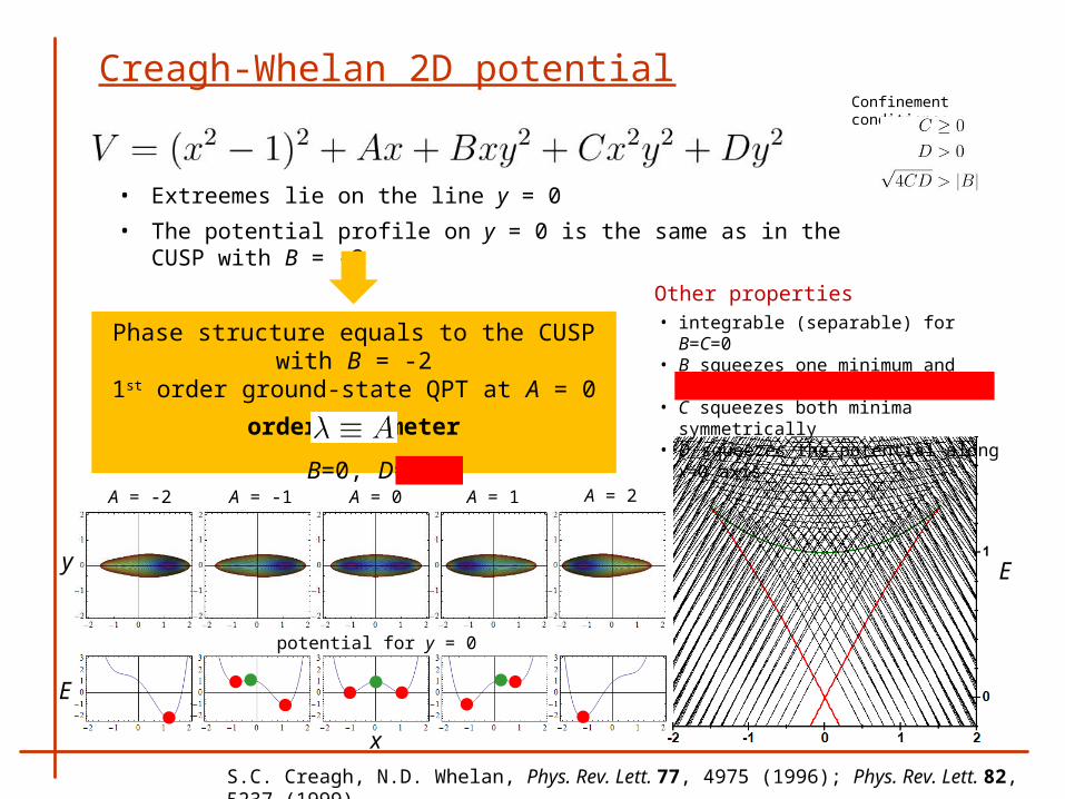
Creagh-Whelan 2D potential
S.C. Creagh, N.D. Whelan, Phys. Rev. Lett. 77, 4975 (1996); Phys. Rev. Lett. 82, 5237 (1999)
• Extreemes lie on the line y = 0
• The potential profile on y = 0 is the same as in the CUSP with B = -2
Confinement conditions:
Phase structure equals to the CUSP with B = -2
1st order ground-state QPT at A = 0
order parameter
• integrable (separable) for B=C=0• B squeezes one minimum and
stretches the other• C squeezes both minima
symmetrically• D squeezes the potential along x=0
axis
Other properties
x
y
potential for y = 0
A = -2 A = -1 A = 0 A = 1 A = 2
E
E
B=0, D=C=4
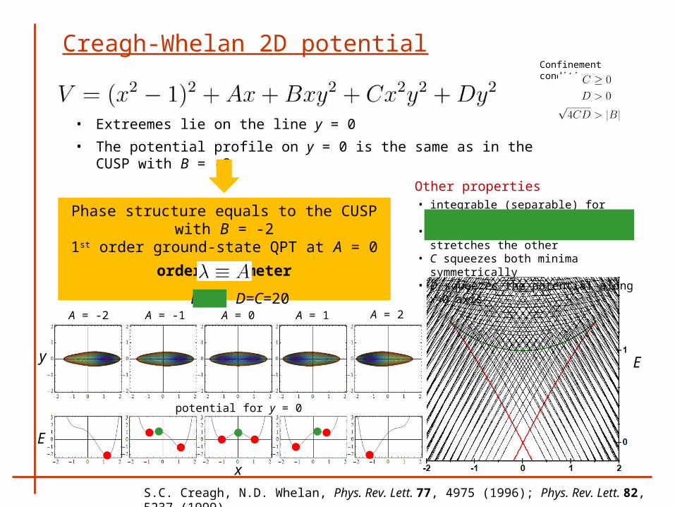
Creagh-Whelan 2D potential
S.C. Creagh, N.D. Whelan, Phys. Rev. Lett. 77, 4975 (1996); Phys. Rev. Lett. 82, 5237 (1999)
• Extreemes lie on the line y = 0
• The potential profile on y = 0 is the same as in the CUSP with B = -2
Confinement conditions:
Phase structure equals to the CUSP with B = -2
1st order ground-state QPT at A = 0
order parameter
• integrable (separable) for B=C=0• B squeezes one minimum and
stretches the other• C squeezes both minima
symmetrically• D squeezes the potential along x=0
axis
Other properties
x
y
potential for y = 0
A = -2 A = -1 A = 0 A = 1 A = 2
E
E
B=0, D=C=20
Creagh-Whelan 2D potential
S.C. Creagh, N.D. Whelan, Phys. Rev. Lett. 77, 4975 (1996); Phys. Rev. Lett. 82, 5237 (1999)
• Extreemes lie on the line y = 0
• The potential profile on y = 0 is the same as in the CUSP with B = -2
Confinement conditions:
Phase structure equals to the CUSP with B = -2
1st order ground-state QPT at A = 0
order parameter
• integrable (separable) for B=C=0• B squeezes one minimum and
stretches the other• C squeezes both minima
symmetrically• D squeezes the potential along x=0
axis
Other properties
x
y
potential for y = 0
A = -2 A = -1 A = 0 A = 1 A = 2
E
E
B=0, C+D=4, D=1
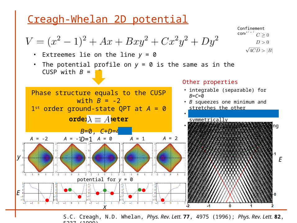
Creagh-Whelan 2D potential
S.C. Creagh, N.D. Whelan, Phys. Rev. Lett. 77, 4975 (1996); Phys. Rev. Lett. 82, 5237 (1999)
• Extreemes lie on the line y = 0
• The potential profile on y = 0 is the same as in the CUSP with B = -2
Confinement conditions:
Phase structure equals to the CUSP with B = -2
1st order ground-state QPT at A = 0
order parameter
• integrable (separable) for B=C=0• B squeezes one minimum and
stretches the other• C squeezes both minima
symmetrically• D squeezes the potential along x=0
axis
Other properties
x
y
potential for y = 0
A = -2 A = -1 A = 0 A = 1 A = 2
E
E
B=0, C+D=4, D=2
Creagh-Whelan 2D potential
S.C. Creagh, N.D. Whelan, Phys. Rev. Lett. 77, 4975 (1996); Phys. Rev. Lett. 82, 5237 (1999)
• Extreemes lie on the line y = 0
• The potential profile on y = 0 is the same as in the CUSP with B = -2
Confinement conditions:
Phase structure equals to the CUSP with B = -2
1st order ground-state QPT at A = 0
order parameter
• integrable (separable) for B=C=0• B squeezes one minimum and
stretches the other• C squeezes both minima
symmetrically• D squeezes the potential along x=0
axis
Other properties
x
y
potential for y = 0
A = -2 A = -1 A = 0 A = 1 A = 2
E
E
B=0, C+D=4, D=4
Creagh-Whelan 2D potential
S.C. Creagh, N.D. Whelan, Phys. Rev. Lett. 77, 4975 (1996); Phys. Rev. Lett. 82, 5237 (1999)
• Extreemes lie on the line y = 0
• The potential profile on y = 0 is the same as in the CUSP with B = -2
Confinement conditions:
Phase structure equals to the CUSP with B = -2
1st order ground-state QPT at A = 0
order parameter
• integrable (separable) for B=C=0• B squeezes one minimum and
stretches the other• C squeezes both minima
symmetrically• D squeezes the potential along x=0
axis
Other properties
x
y
potential for y = 0
A = -2 A = -1 A = 0 A = 1 A = 2
E
E
B=0, D=C=20
Creagh-Whelan 2D potential
S.C. Creagh, N.D. Whelan, Phys. Rev. Lett. 77, 4975 (1996); Phys. Rev. Lett. 82, 5237 (1999)
• Extreemes lie on the line y = 0
• The potential profile on y = 0 is the same as in the CUSP with B = -2
Confinement conditions:
Phase structure equals to the CUSP with B = -2
1st order ground-state QPT at A = 0
order parameter
• integrable (separable) for B=C=0• B squeezes one minimum and
stretches the other• C squeezes both minima
symmetrically• D squeezes the potential along x=0
axis
Other properties
x
y
potential for y = 0
A = -2 A = -1 A = 0 A = 1 A = 2
E
E
B=30, D=C=20
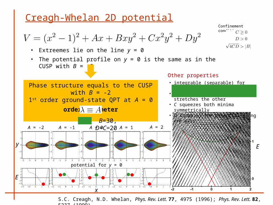
Creagh-Whelan 2D potential
S.C. Creagh, N.D. Whelan, Phys. Rev. Lett. 77, 4975 (1996); Phys. Rev. Lett. 82, 5237 (1999)
• Extreemes lie on the line y = 0
• The potential profile on y = 0 is the same as in the CUSP with B = -2
Confinement conditions:
Phase structure equals to the CUSP with B = -2
1st order ground-state QPT at A = 0
order parameter
• integrable (separable) for B=C=0• B squeezes one minimum and
stretches the other• C squeezes both minima
symmetrically• D squeezes the potential along x=0
axis
Other properties
x
y
potential for y = 0
A = -2 A = -1 A = 0 A = 1 A = 2
E
E
B=39, D=C=20
3. Signatures of ESQPT
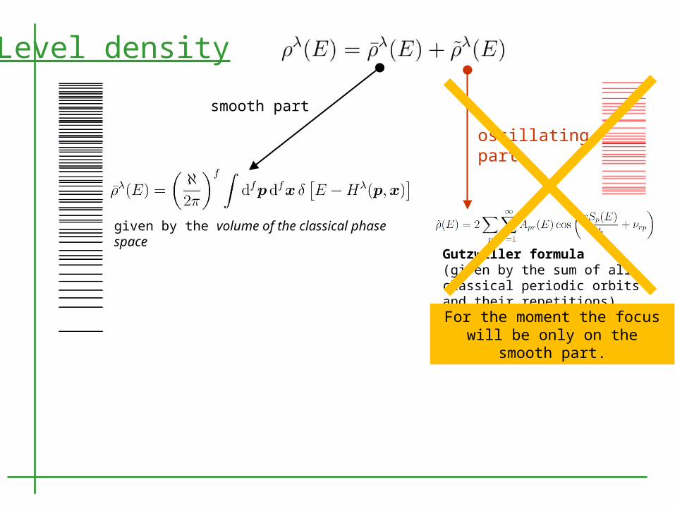
smooth part
given by the volume of the classical phase space
oscillating part
Gutzwiller formula(given by the sum of all classical periodic orbits and their repetitions)
Level density
For the moment the focus will be only on the smooth part.
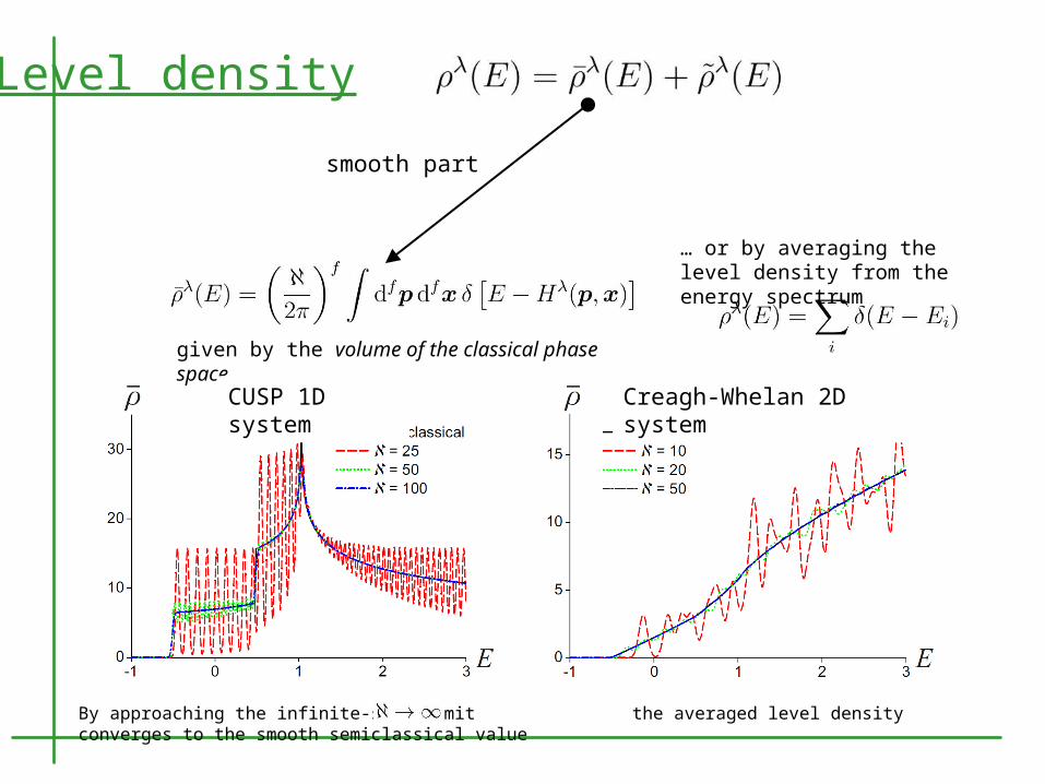
Level density
given by the volume of the classical phase space…
… or by averaging the level density from the energy spectrum
CUSP 1D system
Creagh-Whelan 2D system
smooth part
By approaching the infinite-size limit the averaged level density converges to the smooth semiclassical value
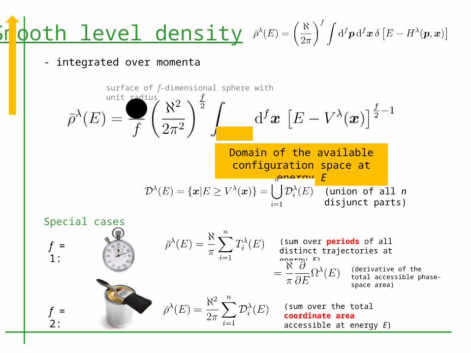
Smooth level density- integrated over momenta
surface of f-dimensional sphere with unit radius
Domain of the available configuration space at energy
E(union of all n disjunct parts)
f = 1:
f = 2:
Special cases
(sum over periods of all distinct trajectories at energy E)
(sum over the total coordinate area accessible at energy E)
(derivative of the total accessible phase-space area)
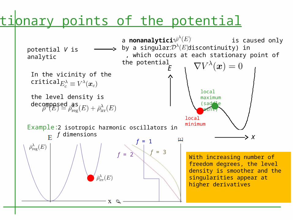
local maximum(saddle point)
local minimum
E
x
Stationary points of the potential
potential V is analytic
a nonanalyticity of is caused only by a singularity (discontinuity) in , which occurs at each stationary point of the potential
In the vicinity of the critical energy
the level density is decomposed as
Example:2 isotropic harmonic oscillators in f dimensions
With increasing number of freedom degrees, the level density is smoother and the singularities appear at higher derivatives
f = 1
f = 3f = 2
k = 4
k = 2 (jump)
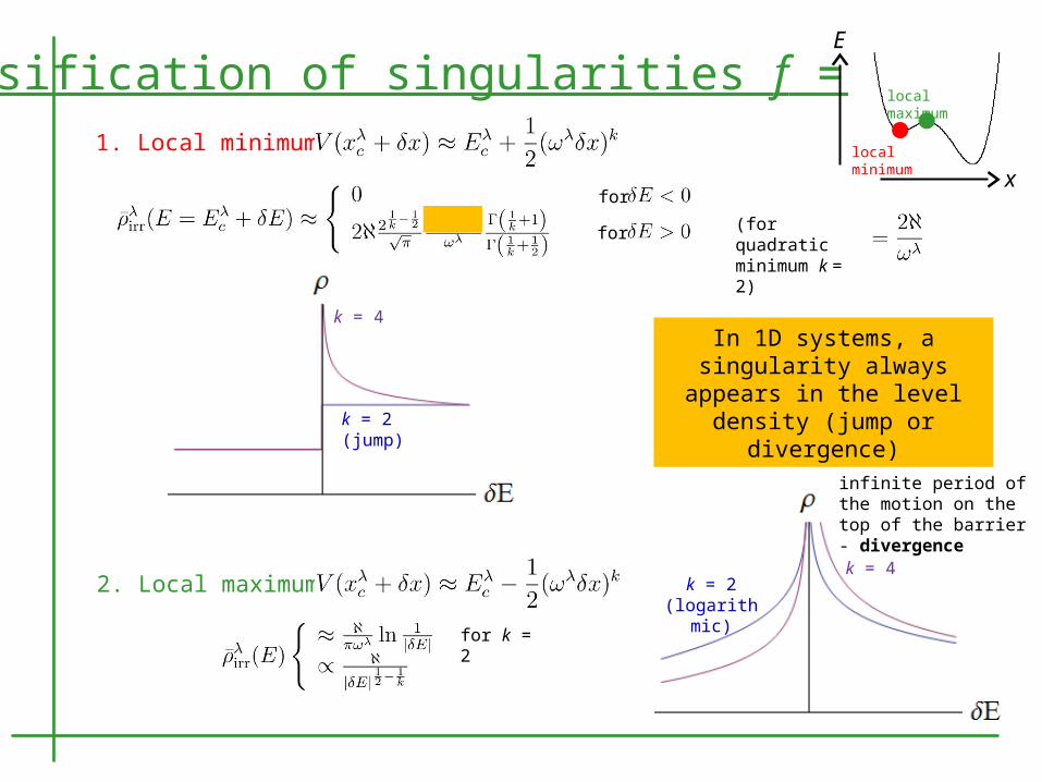
Classification of singularities f = 1local maximum
local minimum
E
x
1. Local minimum
2. Local maximum
(for quadratic minimum k = 2)
for
for
for k = 2
k = 2 (logarithmic)
k = 4
In 1D systems, a singularity always appears in the level density (jump
or divergence)
infinite period of the motion on the top of the barrier - divergence
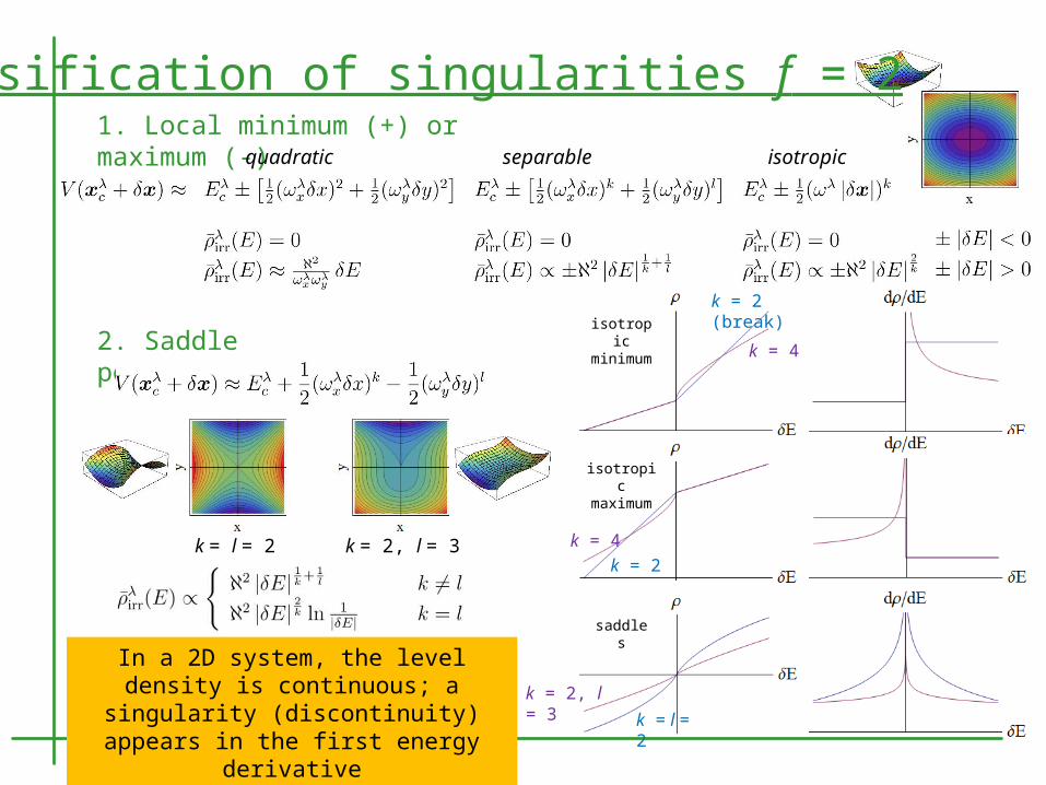
Classification of singularities f = 21. Local minimum (+) or maximum (-)quadratic separable isotropic
k = 4
k = 2 (break)isotropic minimu
m
isotropic maximum
k = 4
k = 2
2. Saddle point
k = l = 2 k = 2, l = 3
saddles
k = 2, l = 3
k = l = 2
In a 2D system, the level density is continuous; a singularity
(discontinuity) appears in the first energy derivative
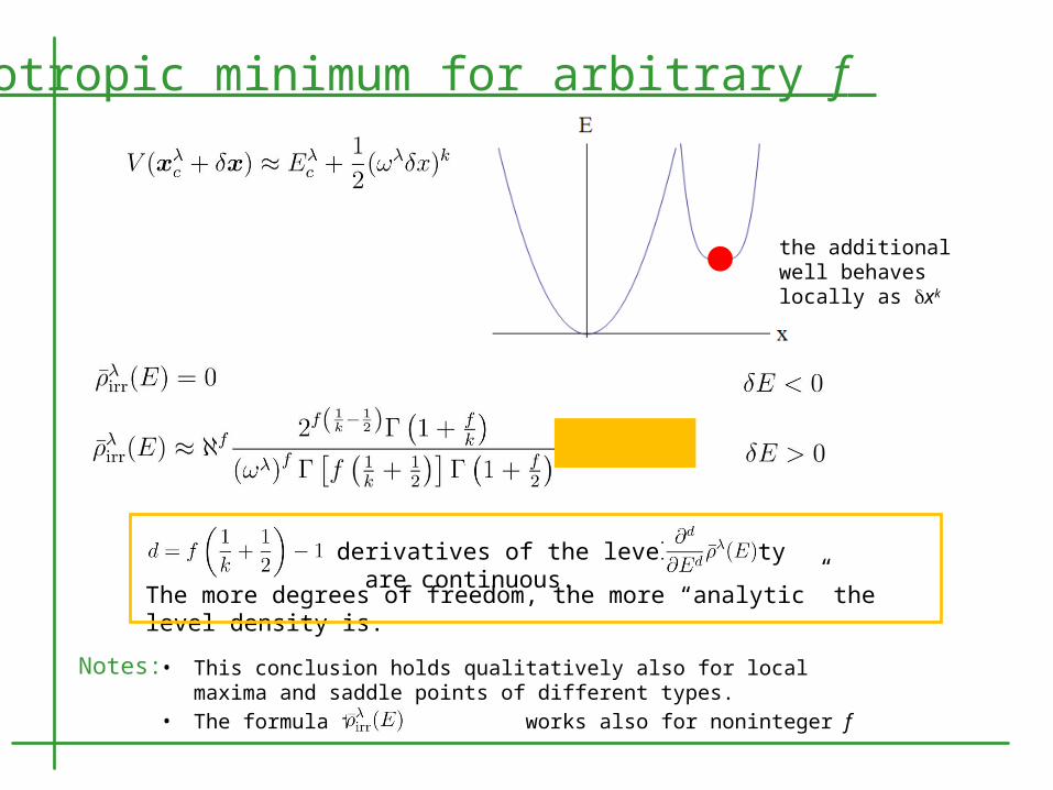
Isotropic minimum for arbitrary f
the additional well behaves locally as xk
derivatives of the level density are continuous.
The more degrees of freedom, the more “analytic” the level density is.
Notes: • This conclusion holds qualitatively also for local maxima and saddle points of different types.
• The formula for works also for noninteger f
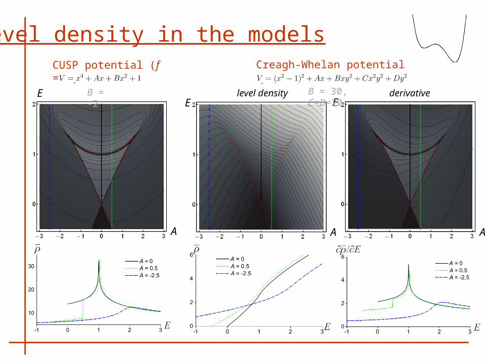
Level density in the modelsCUSP potential (f = 1)
Creagh-Whelan potential (f = 2)
E
A
E
A
level density derivativeE
A
B = -2 B = 30, C=D=20
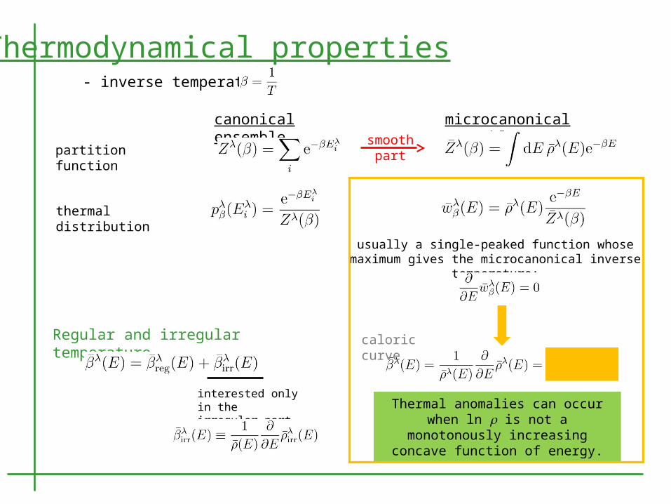
Thermodynamical properties
canonical ensemble
microcanonical ensemble
- inverse temperature
thermal distribution
partition functionsmooth
part
usually a single-peaked function whose maximum gives the microcanonical inverse
temperature:
Thermal anomalies can occur when ln is not a monotonously
increasing concave function of energy.
Regular and irregular temperature
interested only in the irregular part
caloric curve
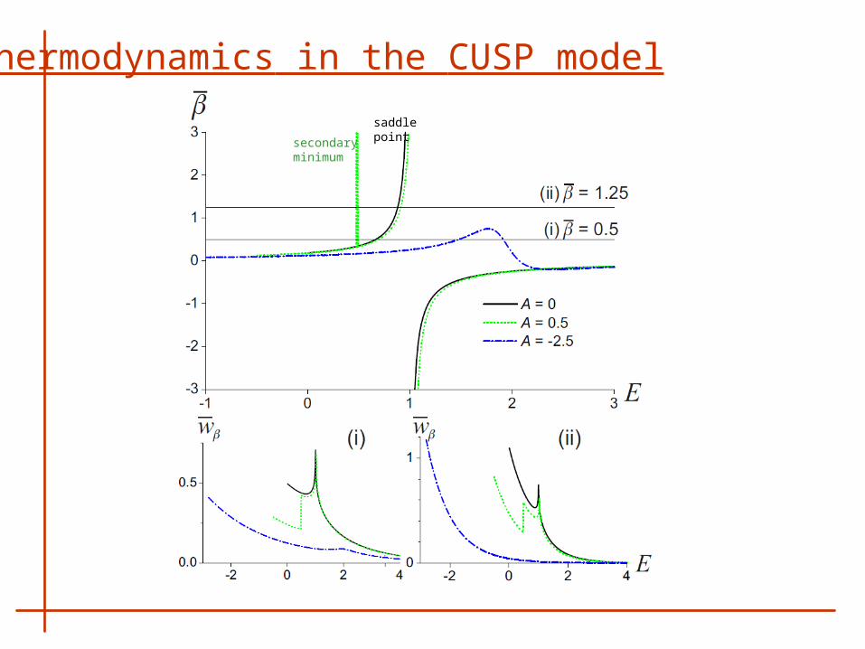
Thermodynamics in the CUSP model
secondary minimum
saddle point
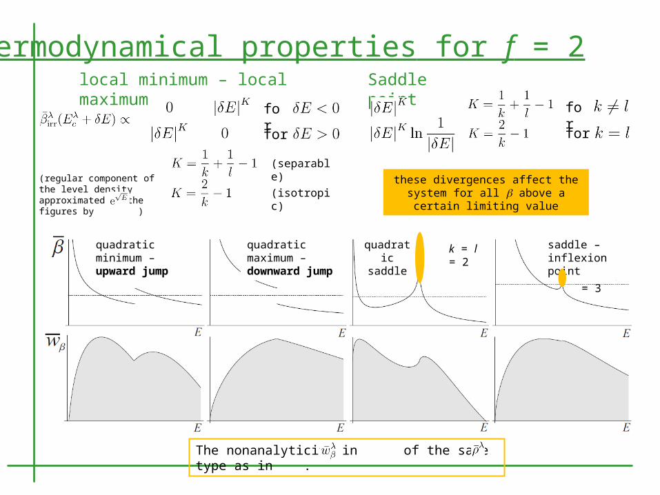
Thermodynamical properties for f = 2local minimum – local maximum
Saddle point
for
for
for
for
(separable)
(isotropic)
quadratic minimum – upward jump
quadratic maximum – downward jump
quadratic saddle
k = l = 2
k = 2, l = 3
saddle – inflexion point
(regular component of the level density approximated in the figures by )
these divergences affect the system for all above a certain
limiting value
The nonanalyticity in of the same type as in .

Thermodynamics in the Creagh-Whelan model
(populated energies in light shades) - higher temperature (lower b) brings the light upper in energy
secondary minimum
saddle point
bimodal, but analytic(away from the critical
region)
Thermal distributions
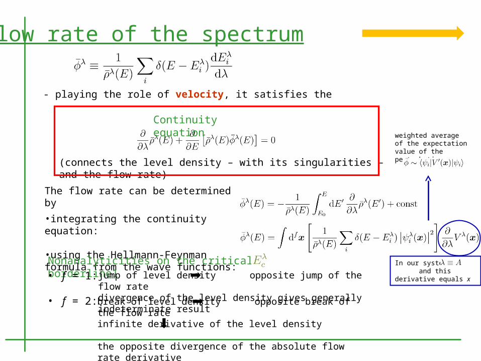
Flow rate of the spectrum
- playing the role of velocity, it satisfies the
The flow rate can be determined by
•integrating the continuity equation:
•using the Hellmann-Feynman formula from the wave functions:
(connects the level density – with its singularities – and the flow rate)
Continuity equation
Nonanalyticities on the critical borderline1• f = 1: jump of level density opposite jump of the flow rate
divergence of the level density gives generally indeterminate result• f = 2: break of level density opposite break of the flow rateinfinite derivative of the level density
the opposite divergence of the absolute flow rate derivative
In our systems and this derivative equals x
weighted average of the expectation value of the perturbation:

Flow rate in the CUSP system
positivepositive (levels (levels rise)rise)
negative negative (levels (levels fallfall))
approximatelapproximatelyy 0 0
vanishes due to the potential symmetry
The wave function localized around the global minimum
Both minima accessible – the wave function is a mixture of states localized around and
Singularly localized wave function at the top of the local maximum with
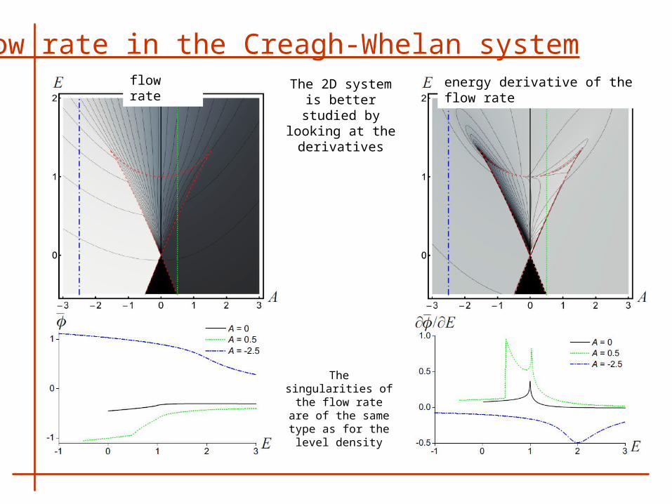
Flow rate in the Creagh-Whelan systemThe 2D system
is better studied by looking at
the derivatives
flow rate energy derivative of the flow rate
The singularities of the flow rate are of the same type as
for the level density
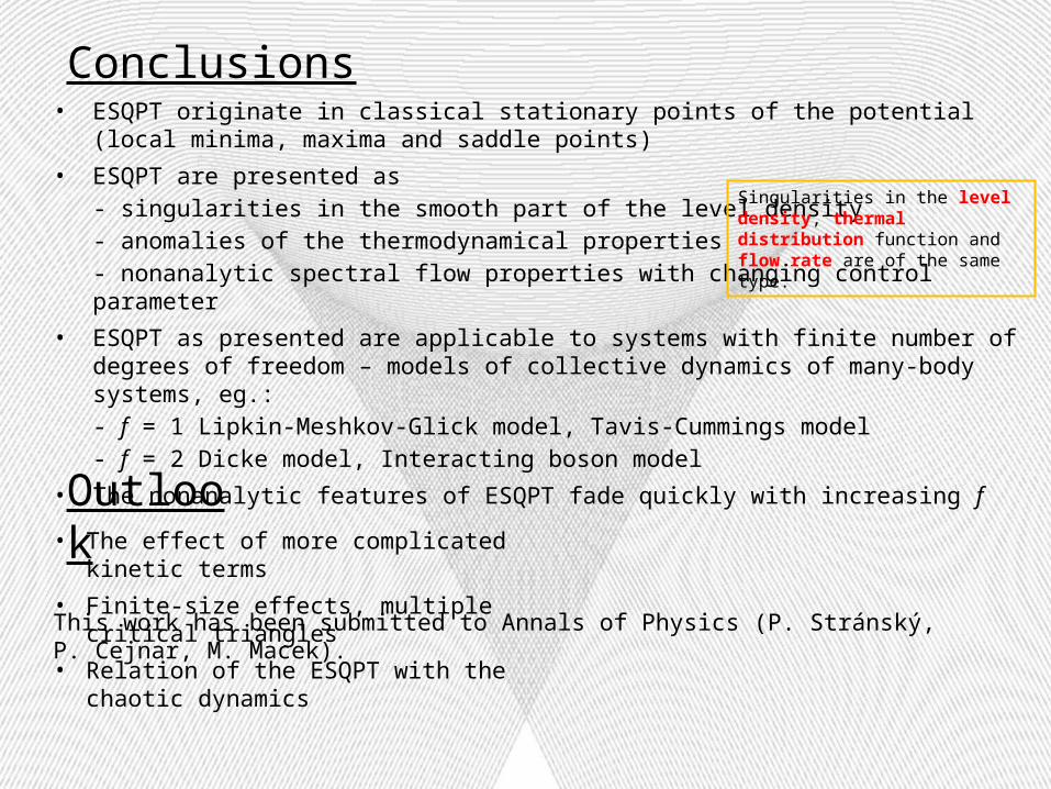
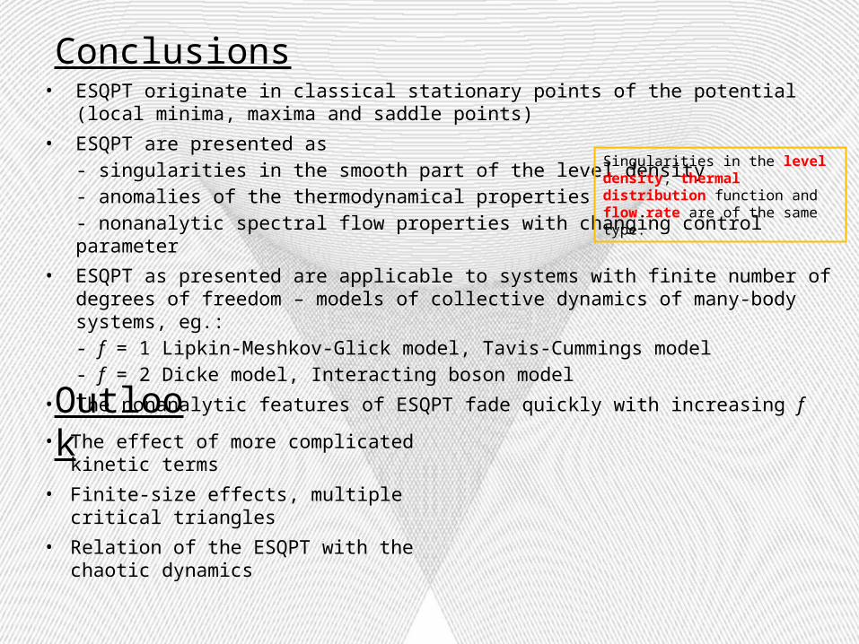
Conclusions• ESQPT originate in classical stationary points of the potential
(local minima, maxima and saddle points)
• ESQPT are presented as - singularities in the smooth part of the level density- anomalies of the thermodynamical properties- nonanalytic spectral flow properties with changing control parameter
• ESQPT as presented are applicable to systems with finite number of degrees of freedom – models of collective dynamics of many-body systems, eg.:- f = 1 Lipkin-Meshkov-Glick model, Tavis-Cummings model- f = 2 Dicke model, Interacting boson model
• The nonanalytic features of ESQPT fade quickly with increasing f
• The effect of more complicated kinetic terms
• Finite-size effects, multiple critical triangles
• Relation of the ESQPT with the chaotic dynamics
Outlook
Singularities in the level density, thermal distribution function and flow rate are of the same type.
This work has been submitted to Annals of Physics (P. Stránský, P. Cejnar, M. Macek).
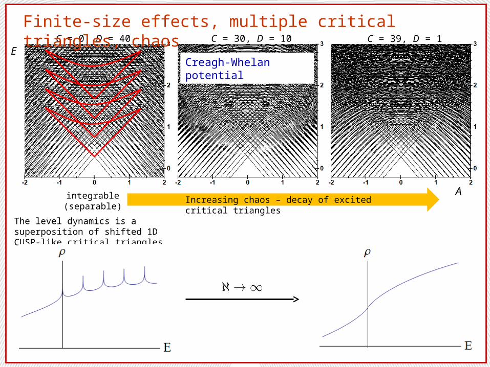
Creagh-Whelan potential
C = 0, D = 40 C = 30, D = 10 C = 39, D = 1
integrable(separable)
Increasing chaos – decay of excited critical triangles
The level dynamics is a superposition of shifted 1D CUSP-like critical triangles
A
E
Finite-size effects, multiple critical triangles, chaos
Conclusions
• The effect of more complicated kinetic terms
• Finite-size effects, multiple critical triangles
• Relation of the ESQPT with the chaotic dynamics
Outlook
• ESQPT originate in classical stationary points of the potential(local minima, maxima and saddle points)
• ESQPT are presented as - singularities in the smooth part of the level density- anomalies of the thermodynamical properties- nonanalytic spectral flow properties with changing control parameter
• ESQPT as presented are applicable to systems with finite number of degrees of freedom – models of collective dynamics of many-body systems, eg.:- f = 1 Lipkin-Meshkov-Glick model, Tavis-Cummings model- f = 2 Dicke model, Interacting boson model
• The nonanalytic features of ESQPT fade quickly with increasing f
Singularities in the level density, thermal distribution function and flow rate are of the same type.
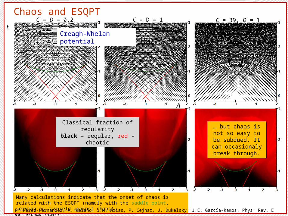
E
Chaos and ESQPTC = D = 0.2 C = D = 1
A
Creagh-Whelan potential
Classical fraction of regularity
black – regular, red - chaotic
Many calculations indicate that the onset of chaos is related with the ESQPT (namely with the saddle point, serving as a shield against chaos)…
C = 39, D = 1
… but chaos is not so easy to be
subdued. It can occasionaly break
through.
… but chaos is not so easy to be
subdued. It can occasionaly break
through.
P. Pérez-Fernández, A. Relaño, J.M. Arias, P. Cejnar, J. Dukelsky, J.E. García-Ramos, Phys. Rev. E 83, 046208 (2011)

Conclusions
• The effect of more complicated kinetic terms
• Finite-size effects, multiple critical triangles
• Relation of the ESQPT with the chaotic dynamicsTHANK YOU FOR YOUR
ATTENTIONMore images on: http://www.pavelstransky.cz/cw.php
Outlook
• ESQPT originate in classical stationary points of the potential(local minima, maxima and saddle points)
• ESQPT are presented as - singularities in the smooth part of the level density- anomalies of the thermodynamical properties- nonanalytic spectral flow properties with changing control parameter
• ESQPT as presented are applicable to systems with finite number of degrees of freedom – models of collective dynamics of many-body systems, eg.:- f = 1 Lipkin-Meshkov-Glick model, Tavis-Cummings model- f = 2 Dicke model, Interacting boson model
• The nonanalytic features of ESQPT fade quickly with increasing f
Singularities in the level density, thermal distribution function and flow rate are of the same type.