dynamics of the stream-power river incision model...

JOURNAL OF GEOPHYSICAL RESEARCH, VOL. 104, NO. B8, PAGES 17,661-17,674, AUGUST 10, 1999

Dynamics of the stream-power river incision model: Implications for height limits of mountain ranges, landscape response timescales, and research needs

Kelin X. Whipple Department of Earth, Atmospheric and Planetary Sciences, Massachusetts Institute of Technology, Cambridge

Gregory E. Tucker Department of Civil and Environmental Engineering, Massachusetts Institute of Technology, Cambridge

Abstract. The longitudinal profiles of bedrock channels are a major component of the relief structure of mountainous drainage basins and therefore limit the elevation of peaks and ridges. Further, bedrock channels communicate tectonic and climatic signals across the landscape, thus dictating, to first order, the dynamic response of mountainous landscapes to external forcings. We review and explore the stream-power erosion model in an effort to (1) elucidate its consequences in terms of large-scale topographic (fluvial) relief and its sensitivity to tectonic and climatic forcing, (2) derive a relationship for system response time to tectonic perturbations, (3) determine the sensitivity of model behavior to various model parameters, and (4) integrate the above to suggest useful guidelines for further study of bedrock channel systems and for future refinement of the stream- power erosion law. Dimensional analysis reveals that the dynamic behavior of the stream-power erosion model is governed by a single nondimensional group that we term the uplift-erosion number, greatly reducing the number of variables that need to be considered in the sensitivity analysis. The degree of nonlinearity in the relationship between stream incision rate and channel gradient (slope exponent n) emerges as a fundamental unknown. The physics of the active erosion processes directly influence this nonlinearity, which is shown to dictate the relationship between the uplift-erosion number, the equilibrium stream channel gradient, and the total fluvial relief of mountain ranges. Similar[y, the predicted response time to changes in rock uplift rate is shown to depend on climate, rock strength, and the magnitude of tectonic perturbation, with the slope exponent n controlling the degree of dependence on these various factors. For typical drainage basin geometries the response time is relatively insensitive to the size of the system. Work on the physics of bedrock erosion processes, their sensitivity to extreme floods, their transient responses to sudden changes in climate or uplift rate, and the scaling of local rock erosion studies to reach-scale modeling studies are most sorely needed.

1. Introduction

1.1. Motivation

Recent recognition of potential global-scale interactions between climate, surface processes, and tectonics [e.g., Adams, 1985; Molnar and England, 1990; Isacks, 1992; Raytoo and Ruddiman, 1992] has sparked the field of tectonic geomorphology and brought the problem of the dynamics of bedrock channel fluvial systems to the forefront of theoretical geomorphology [e.g., Seidl and Dietrich, 1992; Wohl, 1993; Howard et al., 1994; Seidl et al., 1994; Wohl et al., 1994; Zen and Prestegaard, 1994; Montgomery et al., 1996; Tucker and Slingerland, 1996]. Knowledge of the dynamics of bedrock channels is of profound importance for understanding the interaction of tectonics and surficial processes because (1) the channel network defines the texture (plan- view) of the landscape, (2)channel longitudinal profiles

Copyright 1999 by the American Geophysical Union.

Paper number 1999JB900120. 0148-0227/99/1999JB900120509.00

determine much of the relief structure of the landscape, (3) rivers transmit tectonic and/or climatic signals throughout the landscape, and (4) bedrock channels set the boundary conditions for hillslope processes (e.g., soil creep and landslides) responsible for denudation of the land surface. Thus bedrock channels significantly influence both the rates and patterns of erosional unloading in fluvial landscapes and, consequently, long-term sediment fluxes to basins.

Significant progress has been made in developing physically based formalisms for modeling the dynamics of bedrock channel systems [Howard and Kerby, 1983; Seidl and Dietrich, 1992; Anderson, 1994; Howard, 1994; Howard et al., 1994; Kooi and Beaumont, 1994; Rosenbloom and Anderson, 1994; Seidl et al., 1994; Goldrick and Bishop, 1996; Stock, 1996; Tucker and Slingerland, 1996; Stock and Montgomery, 1999]. Of the models that have been proposed, the stream-power (or shear-stress) model is most satisfying as it is cast directly in terms of the physics of erosion [Howard and Kerby, 1983]. The stream-power model is quite general and has been profitably used in a diversity of modeling studies [Anderson, 1994; Howard, 1994; Rosenbloom and Anderson, 1994; Humphrey and Heller, 1995; Moglen and

17,661

17,662 WHIPPLE AND TUCKER: DYNAMICS OF THE STREAM-POWER LAW

Bras, 1995a, b; Goldrick and Bishop, 1996; Tucker, 1996' Tucker and Slingerland, 1996]. This generality, however, brings with it a number of poorly understood parameters whose effective values represent, in the worst cases, a diversity of complex interactions among a suite of physical processes. Given the sweeping generality of the model, its wide- spread use, and the complex nature of the physics of river incision into bedrock, an exploration and sensitivity analysis of the stream-power model seems useful to further development of landscape evolution modeling and as a guide for future field investigations of river incision processes.

l ........ 2 (•e.•h_c,•)•,mi•n .•.,• T( e hc )max

i • BedrOck Channel PrOfile •

?<x max, , 0 10 20 30 40

Distance from Divide (km)

1.2. Approach and Scope

In this paper we review and explore the general stream- power model for bedrock channel profile evolution. Our first aim is to reveal the strengths, weaknesses, and limitations of the current model [e.g., Howard et al., 1994] in a thorough review of its formulation. Further, we aim to illuminate the aspects of the model most critical to modeling the dynamic response of rivers to tectonic or climatic forcing. That is, we explore the role of model parameters in dictating (1) equilibrium channel form, (2) sensitivity of equilibrium channel gradient to rock uplift rate, (3) equilibrium fluvial relief in active orogens, and (4)the timescale of landscape response to tectonic forcing. In this analysis we attempt to develop a relatively complete picture of the dynamic behavior of the stream- power erosion model and, in doing so, develop new insights into the relative importance of the various parameters in the model equations. A dimensional analysis of the bedrock channel evolution equation is used to guide the sensitivity analysis. Limiting assumptions that restrict the "completeness" of our analysis are clearly stated wherever appropriate in the text and are outlined briefly in the paragraph below. Finally we discuss the need for coupled field and modeling studies of bedrock channel systems to place quantitative constraints on those parameters most critical to model behavior, and we discuss some of the physical processes and process feedbacks that set the value of "effective" model

parameters. Howard et al. [1994], Montgomery et al. [1996], and

$klar and Dietrich [1998] have discussed at length the occurrence of bedrock channels in the landscape, the potential controls on bedrock-alluvial transitions, and approaches to modeling these transitions at regional to continental scales. In general, bedrock and mixed bedrock-alluvial channels dominate in headwater regions and in the uplands of tectonically active orogenic belts. We restrict the focus of this paper to the exploration and discussion of fluvially dominated bedrock channel erosion exclusively. Figure 1 is drawn on the basis of stream profile data from the Central Range of Taiwan and serves to define the range and limits of applicability of the stream-power erosion law and hence our analysis. In the Central Range of Taiwan and in the King Range of northern California [Merritts and Vincent, 1989; Snyder and Whipple, 1998; N. Snyder et al., Landscape response to tectonic forcing: DEM analysis of stream profiles in the Mendocino triple junction region, northern California, submitted to Geological Society of America Bulletin, 1999, hereinafter referred to as Snyder et al., submitted manuscript, 1999], the two best examples of active, fluvially sculpted mountain ranges for which we have data, relief is dominated by the elevation drop on fluvially dominated bedrock chan-

0.1

0.01

1E+2

(S c)max _,=L =• ---(•' j=)min -----

Landslides/

Cø11uvialChannels I !! ck'•e (S - constant) Fluvial Bedro

(A c ),rnin !,A,,,,? )max

1 E+3 1 E+4 1 E+5 1 E+6 1 E+7 1 E+8 1 E+9

b Drainage Area (m 2)

Figure 1. Relief structure of active nonglacial orogens based on data from four drainages in the northern Central Range of Taiwan (see Table 1)..(a) Fluvial bedrock channel relief Rf and hillslope/colluvial channel relief Rhc shown along a characteristic divide-to-outlet channel longitudinal profile. The boundary between fluvially dominated bedrock channels and debris flow-dominated colluvial channels, demarcated by Xc is inferred from a break in scaling of the relationship between channel gradient $ and drainage area A (see Figure lb). Here and elsewhere (Table 1) fluvial relief represents 80- 90% of the total relief. (b) Lines schematically represent slope-area data along longitudinal profiles of four Taiwanese rivers. Data for one river are shown for comparison (shaded dots; data are smoothed by log-bin averaging after Tarboton et al. [1991]). Note that concavity estimates reported in Table 1 were derived from regression of raw (unsmoothed) data. The transition from fluvially dominated to colluvial channels is inferred to occur at the break in scaling observed to occur between 105 and 106 m 2 in the drainage area [after Montgomery and Foufoula-Georgiou, 1993]. Minimum and maximum ((Sc)max and (Sc)min) colluvial channel gradients and critical drainage areas ((Ac)max and (Ac)min) represent the range of variability among the four drainages examined and define the range of Rhc indicated in Figure la. Note the log- log scale.

nels (typically 80-90% of total relief; Table 1). Here we make the interpretation, following Montgomery and Foufoula-Georgiou [1993], that the break in scaling observed at a drainage area of 105 - 106 m 2 represents the transition from debris flow-dominated "colluvial" channels to flu-

vially dominated bedrock channels, herein described by a critical downstream distance (Xc; see Figure la). Field observations confirm that the bedrock-alluvial transition is near

the range front in both Taiwan [Hovius et al., 1999] and the King Range [Snyder and Whipple, 1998; Snyder et al., sub-

WHIPPLE AND TUCKER: DYNAMICS OF THE STREAM-POWER LAW 17,663

Table 1. Fluvial Relief Statistics in Active Orogens

Field Area Critical Drainage Area Average Colluvial Slope % Fluvial Relief Concavity Sample Size A a 10•m 2 ½, & Ri/Rt N

King Range, California 0.59 + .20 0.54 + .11 79 + 7 0.40 + .10 14 (high uplift rate) King Range, California 0.72 + .24 0.36 + .05 80 + 5 0.49 + .10 7 (low uplift rate) Central Range, Taiwan 1.40 + .48 0.63 + .26 89 + 6 0.41 + .10 4

All uncertainties indicate 1-sigma error bars. aAc deftned by break in slope-area scaling in longitudinal profile data (only). bThe condition 0 = m/n holds if and only if channels are in equilibrium and both U and K are constants. Reported values

were fit to long profile data between Ac and the bedrock-alluvial transition only.

mitted manuscript, 1999]. In other landscapes, fluvially dominated bedrock channels constitute a considerably smaller fraction of the total relief [e.g., Montgomery and Foufoula-Georgiou, 1993; Sklar and Dietrich, 1998], but we believe the two examples in Table 1 are typical of nonglacial tectonically active mountain ranges.

Sklar and Dietrich [1998] give a cautionary note on range of applicability of the stream-power erosion law that high- lights some aspects of the dynamics of bedrock channels that are beyond the scope of our analysis. We restrict our analysis to the fluvially dominated part of the bedrock channel system, specifically avoiding debris flow-dominated channel tips. In addition, we do not address the retreat of large-scale knickpoints that Seidl et el. [1996] argued may be limited by rock mechanics and weathering rather than fluvial erosion. Fur- ther, we intentionally restrict our discussion to fluvial landscapes, making no mention of the role of glacial erosion.

2. The Shear-Stress/Stream-Power Erosion Model

The detachment-limited rate of bedrock channel erosion e

is often modeled as a power law function of drainage area A and stream gradient S:

E =KAmS n (1) where m and n are positive constants and K is a dimensional coefficient of erosion (dimensions of all variables are listed in the notation section). The drainage area term appears as a proxy for discharge. Howard and Kerby [1983] showed that local erosion rates derived by differencing channel profiles resurveyed over a 7-year interval in rapidly eroding badlands were well explained by a formulation of (1) assuming incision rates linearly proportional to bed shear stress (m -- 1/3 and n -- 2/3).

Since that time, various formulations of (1) have been used extensively in modeling studies of bedrock profile evolution [ Seidl and Dietrich, 1992; Anderson, 1994; Howard, 1994; Rosenbloom and Anderson, 1994; Seidl et al., 1994; Humphrey and Heller, 1995; Moglen and Bras, 1995a, b; Tucker and Slingerland, 1996, 1997; Sklar and Dietrich, 1998]. Other bedrock channel erosion laws have been formu- lated [e.g., Beaumont et al., 1992; Kooi and Beaumont, 1994] but are less readily cast in terms of the physics of observed erosion processes. Therefore, although these other

erosion laws have been incorporated into modeling studies that have yielded useful insights about landscape evolution, we do not pursue their dynamics here. In the paragraphs below we review the derivation of (1) in order to highlight the underlying assumptions and to emphasize relations between effective parameters k, n, and m and physical variables such as process (e.g., plucking versus abrasion), lithology, climate, sediment loading, and drainage basin shape. Under- standing these process-parameter linkages and how they influence model predictions is essential to critical evaluation and further refinement of landscape evolution simulations as well as to the formulation of effective field and laboratory research efforts in the area of bedrock channel erosion processes.

Derivation of (1) starts with the reasonable postulate that erosion rate is a power law function of shear stress xb or, alternatively, stream power per unit area of channel bed (the product of shear stress and mean velocity V, henceforth "unit stream power"). These basic postulates are written:

Shear stress œ = kbxb a (2a) Unit stream power •; = kb('lJbV) a (2b)

Where kb and a are positive constants. Note that ko is a dimensional constant with dimensions that depend on both the exponent a and whether the shear-stress or unit stream- power formulation is used (see notation section). Both forms of (2) implicitly assume that the threshold (e.g., critical shear stress) is negligible for the flows of interest. An erosion threshold term can easily be incorporated into numerical solutions and has some interesting effects [Howard, 1997; Tucker and Slingerland, 1997] but is omitted here in keeping with standard formulation of the stream-power law and in the interest of obtaining analytical solutions. Coefficient ko depends on rock mass quality (lithology, jointing, and weathering), sediment loading, and process. Similarly, the exponent a likely depends on the dominant process and has been argued to range from 1 to as much as 7/2 [Hancock et al., 1998; K. Whipple, et el., River incision into bedrock: Mechanics and relative efficacy of plucking, abrasion, and cavitation, submitted to Geological Society of America Bulletin, 1999, hereinafter referred to as Whipple et el., submitted manuscript, 1999]. Thus, for the range of erosion processes adequately described by (2) the exponent a, in particu-


lar, carries information about the physics of the erosion process.

Several researchers have recently argued that erosion rate is a function of the ratio of sediment flux qs to sediment transport capacity qc [Sklar and Dietrich, 1997; Slingerland et al., 1997; Sklar and Dietrich, 1998], which likely varies with uplift rate, climate, and position in a catchment. A simple way to denote this dependence within the framework of the stream-power erosion law is to write

kb = kef(qs,qc) (3) where ke depends on rock mass quality and erosion process and j(qs,qc) is an unspecified function. As argued by Sklar and Dietrich [1998], the role of sediment flux (here denoted as j(qs,qc)) encapsulates at least two competing effects: (1) ac- celerated erosion due to an increased number of tools in the

flow and (2) reduced erosion as a result of partial shielding of the bed from particle impact and other processes. For the sake of simplicity and in keeping with the standard formulation of the stream-power law we restrict our analysis to the condition of constant kb (for a given lithology), an assumption incorporated into most landscape evolution models.

Coupling either (2a) or (2b) and (3) with relations describing flow hydraulics, channel geometry, and basin hydrology results in a simple expression for channel erosion rate in terms of stream gradient and drainage area, in the form of(1). In this analysis, hydrologic and hydraulic variables (discharge Q, flow depth D, flow width W, flow velocity V, shear stress '•b, and erosion rate œ) are taken as time-averaged quantities, such that discharge can be taken as a simple function of drainage area A. Thus it is implicitly assumed that an effective discharge can be defined that adequately represents the integrated effects of the full-time history of flood discharges [Wolman and Miller, 1960; Willgoose, 1989; Tucker and Bras, 1997]. Given this assumption, the internal relations are conservation of mass (water)

Q = VDW (4) conservation of momentum (steady and uniform flow) in wide channels

hydraulic geometry 'c!• = pgDS - pC fV 2 (5)

W = Ic•Q • and a relation for basin hydrology

(6)

Q = kqA c (7)

In the above, p is density of water, g is gravitational acceleration, CS is a dimensionless friction factor, k• and kq are dimensional constants, and b and c are positive dimensionless constants. For convenience, the small-angle approximation (sintz -- tantz) has been exploited to write shear stress in terms of the streamwise gradient S. Constants kw and b depend on rock mass quality, erosion process, sediment loading, and hydraulic resistance C s. Constants kq and c are a function of climate, runoff processes, the return period of the effective discharge, and basin topology.

Equation (6) is well known empirically for alluvial channels fi'om the hydraulic geometry literature [Leopold and Maddock, 1953] (b-- 1/2). Similar values of the exponent b appear to apply to partially alluviated bedrock channels

[Hack, 1973], a value consistent with approximately logarithmic channel profiles observed in nature [Hack, 1957]. However, besides the pioneering work of Suzuki [1982], no comprehensive study of the controls on bedrock channel width has been done.

Combining (2) -(7), the bedrock erosion rate for shear- stress dependent erosion can be written as

œ = rA2aC(1-b)/3S2a/3 (8a) K k•k• 243 2•(1-o)/3f(q,)C?p•g2•/3 (8b) = kq

Comparing (8) with (1), it can be seen that exponents rn and n are related to erosion process, hydraulic geometry, and basin hydrology according to

m= 2ac(1- b)/3 n= 2a/3

•C --

(9a)

(9b)

(9c)

Similar results are readily found for the unit stream-power case

K - kek•ak•(1-t•)f(qs)paga m=ac(1-b)

Thus the shear-stress and unit stream-power versions of the erosion law differ in detail but are not fundamentally different. Moreover, given that the exponent a in (2) is unknown, it would be difficult at present to discriminate between the unit stream-power and shear-stress models on the basis of field data.

Equations (8b) and (lea) emphasize the multivariate controls on the effective coefficient of erosion K in (1) and convey the relative sensitivity of K to lithology, climate, and sediment load. Within the broad subset of fluvial erosion

processes adequately described by (2) -(7), the m/n ratio discussed by Seidl and Dietrich [1992], Moglen and Bras [1995b], Dietrich et al. [1996], Tucker [1996], and others is shown by (9) and (le) to be independent of the dominant erosion process (e.g., plucking versus abrasion), depending only on the relative rates of increase of discharge with drainage area and of channel width with discharge regardless of whether one accepts a shear-stress or unit stream-power formulation. For typical values of the exponents in (6) and (7) (0.7 _< c _< 1 and b -- 0.4 - 0.6) the m/n ratio is predicted to fall into a narrow range near 0.5 (0.35 < m/n < e.6), consistent with empirical values derived fi'om field data [Howard and Kerby, 1983] and many derived fi'om map data relating channel gradient and drainage area (see Table 1) [Flint, 1974; Tarboton et al., 1989; Willgoose et al., 1990; Tarboton et al., 1991; Willgoose, 1994; Moglen and Bras, 1995b; Slingerland et al., 1998]. Although the m/n ratio is known to strongly influence the concavity of equilibrium channels [e.g., Moglen and Bras, 1995a], many additional factors can affect profile concavity. Thus the restriction that the m/n ratio should fall in a narrow range does not necessarily imply that channel concavities are likewise restricted. Indeed, em-

(lea)

(10b)

(10c)

(led)


pirical estimates of channel concavity (often equated to the m/n ratio) outside the expected range have been reported in some landscapes [e.g., Sklar and Dietrich, 1998] and probably reflect some combination of disequilibrium conditions, systematic downstream variations in either rock uplift rate or erodibility K, or regression of data that cross the bedrock- alluvial transition.

3. Nondimensionalization

It is useful to express the governing equation for the evolution of bedrock channel profiles in terms of dimensionless variables. This allows a preliminary scaling analysis of the evolution equation and simplifies analysis of the dynamics of river profile response to external forcings (e.g., tectonics or climate). Willgoose et al. [1991] give a nondimensionalization scheme for their transport-limited equation set, which is similar in spirit to the one presented here. In addition, Fernandes and Dietrich [1997] present a similar dimensional analysis of equations describing hillslope evolution by diffusive processes.

For a detachment-limited system (i.e., bedrock channels), conservation of mass (rock) dictates the form of the channel profile evolution equation:

dt

where z is the elevation of the river bed, x is the distance downstream, and U is the rock uplift rate defined relative to the erosional base level. Combining (11) with (1) and em- ploying Hack's law [Hack, 1957],

A = k•x • (12) where k, is a dimensional constant and h is the reciprocal of the Hack exponent, shows that river profiles are governed by a nonlinear kinematic wave equation [Whitham, 1974]:

- (x,O -amxhmn-'l- I Xc -< X -< r dt

with wave speed -Kk, mXhmS •4, where S = I(az/ax)l, L is the bedrock channel stream length measured from the divide, and the area-length exponent h is seen to vary over a narrow range fi'om 1.67 to 1.92 [Hack, 1957; Marltan et al., 1996; Rigon et al., 1996].

Nondimensionalization of the bedrock river profile evolution equation first requires that we write (13) in general terms:

z F(U,K,k a dx ) = • t (14) ,x, dz'

The right-hand side of (14) has six independent variables in two dimensions (length and time), which therefore can be written as four independent nondimensional groups. Note that the exponents h, m, and n do not appear as variables on the right-hand side as these are part of the unspecified function F. Similarly, the variable Xc introduced earlier (see Fig- ure 1) does not appear as this enters only as a boundary condition to the unspecified function F. In order to proceed with the nondimensionalization we introduce three representative scales (H, L, and Uo) to define the following dimensionless variables:

z x U tU o z,=-- x,--- U,= t,=• (15) H L U o H

U o = U'(x,t) (16) where H and L are the representative vertical and horizontal length scales, respectively, and an asterisk is used to denote all dimensionless variables. The choice of H/Uo as a characteristic timescale is convenient and assures that the dimen-

sionless rate of bed elevation change (dz,/dt,) is of order unity:

dz, 1 dz

dt, = U'•'•' (17) The length scale H need not be equal to the bedrock fluvial relief Rf, though this makes a convenient choice if known.

The fourth and final dimensionless group on the right- hand side must involve the variables U, K, and k,, and can be determined readily by rewriting (13) in terms of the dimensionless variables defined above:

dz, = S, _ NE-lx, hml dz, ) n where the dimensionless uplift-erosion number N• is given by

Uo k•-mLn-hmH-n N/r =-•- (19)

Note that by definition, if the rock uplift rate U is steady and uniform, the dimensionless uplift rate U, is unity (equations (15) and (16)).

The uplift-erosion number can be immediately identified as the critical dimensionless group governing the dynamics of the bedrock channel profile evolution equation (18). More- over, as with the familiar Reynolds and Froude numbers in fluid mechanics, dynamic responses associated with perturbations of the suite of variables Uo, K, ka, L, m, and H can be fully captured by simply considering responses to perturbations in the uplift-erosion number NE. For instance, changes in the rock uplift relative to base level U are dynamically equivalent to changes in the coefficient of erosion K. In addition, covariance of empirically determined K values and the exponent m (the dimensions of K depend on m) [Sklar and Dietrich, 1998; Stock and Montgomery, 1999] does not complicate the dynamic behavior of the profile evolution equation as this effect is encapsulated within the uplift- erosion number. Consideration of steady state conditions will reveal the roles of the exponents h, m, and n in the form and dynamics of modeled river profiles.

4. Steady State River Profiles

In this section we explore the behavior of bedrock channels as predicted by the shear-stress/stream-power model in order to draw out the significance of the issues outlined earlier in regard to channel profile form, the relationship between equilibrium channel gradient and environmental controls (climate, lithology, and uplift rate), and the equilibrium height of mountain ranges. In the analysis these environmental controls are all represented by the uplift-erosion number NE introduced in section 3, which can be quantita- tively interpreted as either reflecting tectonic forcing (through Uo) or climatic and lithologic forcing (through K).


4.1. Equilibrium Channel Gradient

At steady state the river profile is by definition invariant in time (dz/dt = 0 and dz,/dt, = 0). Local erosion rate œ must everywhere balance the rock uplift rate. Setting dz,/dt, equal to zero and solving for dimensionless stream gradient S,, the steady state solution of (18) is readily obtained:

(dZ*)NEl/ns,l/nx,-hm/n s,= = (20) Equation (20) shows that the slope exponent n largely dictates the sensitivity of stream gradient to changes in rock uplift rate, lithology, and climate (Figure 2). Equilibrium fluvial relief will be shown later (equation (22)) to scale precisely with the stream gradient and therefore is included in Figure 2 for convenience. Because only the sensitivity of the equilibrium gradient to differences in climate or uplift rate is of interest here, channel gradients are reported relative to a reference condition NEr calculated using the parameters listed in Table 2, reported here for completeness, although the actual values used are inconsequential. This convenient arti- fice is used throughout the paper to normalize illustrative plots with no loss of generality. For the restricted case of uniform block uplift (U is constant), uniform coefficient of erosion (K is constant), and no downstream changes in erosion process (n and m are constant), the dimensionless uplift rate U, is unity, and the uplift-erosion number captures all the dependencies of channel gradient on the rock uplift rate, lithology, and climate.

As exemplified by (19) and (20), the equilibrium gradient of a bedrock channel reflects a balance between the rate of rock uplift U and the rate of channel incision per unit slope and area K. Importantly, the steepness of a river profile depends on the uplift-erosion number raised to a power given by the reciprocal of the slope exponent (l/n) (Figure 2). The significance of this fundamental prediction of (1) has not yet been widely appreciated [Tucker and Bras, 1998]. For a lin-

'- 100 / 100

..... n : 2/3 / • 10 n=l / 10 o n=2 / ...

E 0.1 o.1 ::] / / ill: ß - / ß __-- /

'-• 0 01 ' ' ' •'"1 ........ ', ........ ', ....... 0.01 O' '

0.01 0.1 1 10 100

Uplift/Erosion Ratio (N E/[N E ] r )

Figure 2. Sensitivity of dimensionless equilibrium channel gradient and dimensionless equilibrium fluvial relief to the uplift-erosion number NE as a function of the slope exponent n. In order to emphasize the sensitivity to changes in the uplift-erosion number both dimensionless channel gradient and dimensionless fluvial relief are shown relative to a reference value noted with the subscript r. Reference values in all figures are computed with the parameters listed in Table 2. Note the log-log scale.

Table 2. Parameter Values Used in Examples

Parametera Value Dimensions Notesb

œ 2],500 ILl --- H 2,900 [L] --- xc 320 [L] 105 m 2 source area k, 6.69 [L 2'h] Hack [1957] h 1.67 [ ] Hack [1957] m/n 0.50 [] --- K (n = 1) 2.00 x 10 -s [m]'2m yr '•] SS K (n = 2/3) 9.28 x 10 's [m•'2m yr '•] SS K (n = 2) 2.00 x 10 -s [m•'2• yr '•] SS

aAll in mks units, except K as noted. bSS denotes Ks chosen to yield equivalent steady state profiles

for U = 2 mm yr-1 for all n (for convenience only).

ear erosion process (a = 1, equation (2) and n = 2/3, equation (9)), equilibrium channel gradient is very sensitive to changes in the uplift-erosion number. For a slightly nonlinear erosion process (n = 1, equation (9)), equilibrium channel gradient is linearly related to the uplift-erosion number. Finally, for a highly nonlinear process (n > 1, equation (9)), equilibrium channel gradient is only weakly dependent on the uplift-erosion number (Figure 2).

Thus landscape response to tectonic regime is critically dependent on the slope exponent n. The direct dependence of the slope exponent n on the physics of fluvial bedrock erosion (equations (2), (9), and (10)) is powerful testimony to the need for field studies of these processes. Moreover, the m/n ratio plays no direct role in the sensitivity of channel gradient and relief to the uplift-erosion number NE.

4.2. Equilibrium Longitudinal River Profiles

4.2.1. River profile concavity. Assuming simple block uplift (dU/dx = 0) and uniform lithology, precipitation, and erosion process (dK/dx = 0; m and n are constants), (18) can readily be integrated to derive an expression for dimensionless streambed elevation z, as a function of dimensionless

distance downstream x,:

--½ 1 (21a)

z,(x,)-z,(1)-NE1/nu,1/nln(x,) hm-1 (2lb) where L is total bedrock stream length and z,(1) is the dimensionless elevation at the basin outlet (or at the bedrock- alluvial transition). Equations (21a) and (2lb) are valid for X,c _< x, _< 1 only, where X,c is the dimensionless distance downstream fi'om the divide at which fluvial processes become dominant [Montgomery and Foufoula-Georgiou, 1993] (See Figure 1).

Although calculations using the restrictive assumptions incorporated into (2 la) and (2 lb) are illustrative (Figure 3), we stress that nonuniform uplift rates [i.e., Adams, 1985; Koons, 1989], orographic precipitation [Beaumont et al., 1992; Masek et al., 1994b], and systematic downstream


1

• '"• 0.6 =

o., • 0.2 Z

0

0 0.2 0.4 0.6 0.8 1

Dimensionless Distance (x I L )

3 1\..

•"•. .... ß ...... schematic ridge •' I!\. --- '-.. / profile • 2 ul-:"• • ..... \ '-,•-'---_1•

I', % .... x •,R hc --",.

o

0 x c 5 10 15 20 25

Distance from Divide (km)

4

• n =1 mm ' 3

• 'g 1

0

0 25 50 75 100

c Range Half Width (L) (km)

Figure 3. Equilibrium channel profiles and fluvial relief (assuming spatially constant U, K, m, and n). (a) Longitudi- nal profile concavity is controlled by the hm/n ratio (concavity index). Exponent h is held constant at the observed value of 1.67 [Hack, 1957]. Natural channels are approximately logarithmic in form: consistent with h = 1.67- 1.92 and m/n = 1/2. (b) At steady state the topographic envelope of mountain ranges is set by the longitudinal profiles of the stream network plus the relief on hillslopes and colluvial channels (Rhc). A theoretical profile, in dimensional form (trunk channel' solid black line; tributary channels (projected into plane)' dashed black lines), computed with U = 5xl 0 -3 ma -], K = 1.2x10 -s, and n = 1 (other parameters as listed in Table 2) is shown (for Xc _( x _(L) for direct comparison against data for a divide-to-outlet longitudinal profile (trunk channel only) for an intermediate-sized basin in northern Taiwan (Table 1). Stair steps in the profile from Taiwan probably reflect noise in the digital elevation data. (c)Dimensionless fluvial relief increases slowly with range half width L for all values of n and uplift-erosion number NE (shown for n = 1).

variations in sediment loading in streams [Sklar and Dietrich, 1997; Slingerland et al., 1997; Sklar and Dietrich, 1998] all play potentially important roles in even the simplest realistic scenario. For steady, uniform uplift, constant coefficient of erosion, and constant area and slope exponents (m and n) the ratio hm/n dictates the equilibrium form of river profiles (Figure 3a). For typical values of h (1.67 < h < 1.92) and the rn/n ratio (0.35 < rn/n < 0.6) the ratio hrn/n ranges fi'om 0.58 to 1,15, and predicted river profiles are approximately logarithmic, as documented by Hack [1957] and illustrated in Figure 3b.

Although the steady state form (concavity) of river profiles subjected to the constraints outlined above is predicted to be relatively insensitive to the multivariate controls on bedrock erosion processes, any deviations fi'om steady state, or any systematic downstream changes in uplift rate (e.g., tilting) or erodibility (e.g., change in dominant process, sediment supply, and cover)will complicate the interpretation of river profile data in terms of the m/n ratio. For instance, where uplift rate increases monotonically downstream (dU/dx > 0; back-tilting), profile concavity will be diminished and vice versa where uplift rate decreases downstream (dU/dx < 0). In addition, spatially variable controls on erodibility (K)may play an important role in channel profile form [Sklar and Dietrich, 1998]. Because of such difficulties, Seidl and Dietrich [1992] proposed a method for extracting rn/n ratios from differences of channel and tributary gradients at tributary junctions. Although their analysis did not account for possible differences in alluvial cover or channel width between

tributary channels, their method requires no assumptions regarding steady state or equilibrium conditions. However, their finding of m/n = 1 for streams in the Oregon Coast Range is at odds with other data (i.e., reasonable values for exponents in (6) and (7) and logarithmic channel profiles) and has not yet been explained.

4.2.2. Equilibrium fluvial relief and the height of mountain ranges. Over long timescales the height of mountain ranges is limited by either crustal strength [e.g., Molnar and Lyon-Caen, 1988; Bird, 1991; Masek et al., 1994a] or by a balance between rock uplift and erosion [e.g., Adams, 1985; Koons, 1989], whichever is more restrictive. In the case where crustal strength is not limiting, the equilibrium height of a fluvially sculpted mountain range is dictated by four fun- dmental geomorphic controls: (1) range width, (2) longitudinal profiles of transverse bedrock streams, (3) the length and gradient of colluvial channels above the fluvial network, and (4)the length (= drainage density) and gradient of hillslopes (see Figure 1).

Equilibrium fluvial bedrock channel relief Rf is given by the difference between the elevation at the headwater of the

fluvial channel (i.e., at x = Xc) and the elevation of the basin outlet or the bedrock-alluvial channel transition (i.e., at x = L). In terms of dimensionless variables, from (21), fluvial bedrock channel relief is given by

g,f : NE1/ns,1/nll-•!-l(1 - X,c 1-hm/n) hrn

½1 n

(22a)

R,f =-NE1/nu, 1In lnx, c hm = 1 (22b) n


Unsurprisingly, equilibrium fluvial relief varies in exactly the same way with the uplift-erosion number NE as does the equilibrium channel gradient (see Figure 2). Thus the slope exponent n in (1) emerges once again as a critical unknown. Recall that in the case of uniform rock uplift the dimensionless uplift rate U, is unity, and the uplift-erosion number fully captures the dependence of fluvial relief on environmental controls (lithology, climate, tectonics, and basin size). Thus fluvial relief depends on rock uplift rate to the 1/n power, the coefficient of erosion to the -1/n power, and stream length to a small power (-0.15 - 0.42 for typical values of hm/n), as illustrated in Figures 2 and 3c. In plotting Figure 3c it is assumed that the largest transverse drainages (length L) scale with range half width.

Equation (22) makes the direct prediction that all else being equal, greater relief is expected for lower values of the coefficient of erosion K. That is, greater relief is expected for more resistant lithologies and lower precipitation rates. Although this result is not surprising, it runs counter to fre- quent arguments in the literature that greater precipitation leads to greater relief [e.g., Fielding et at., 1994; Masek et at., 1994b].

Theoretical mainstream and tributary profiles calculated with (21a) are plotted in Figure 3b in dimensional form for direct comparison with data from a channel typical of those draining the northern Central Range of Taiwan. In this and other tectonically active, fluvially sculpted landscapes (see Table 1 and Figure 1)the total relief is dominated by the elevation drop of bedrock channels, and equilibrium range crest elevation can be expected to vary strongly with the fluvial relief. Moreover, Schmidt and Montgomery [1995] have argued that hillslope relief rapidly attains a maximum in actively incising landscapes. Where this condition holds, the relationship between uplift rate, climate, and range crest elevation above base level can be described to first order by (22). However, drainage density may decrease with rock uplift rate [e.g., Howard, 1997; Tucker and Bras, 1998], resulting in longer hillslopes and possibly greater hillslope relief (and proportionately reduced fluvial relief). In addition, little is at present known about the controls on either the length (represented by Xc)or gradient of debris flow- dominated channels [Howard, 1998]. Thus, although equilibrium range crest elevation in fluvially dominated landscapes can be described to first order by (22), this relationship strictly relates only to the fluvial relief.

5. Transient Response to Tectonic Forcing

Thus far we have considered only equilibrium (steady state) channel profiles. Here we address the questions: (1) under what conditions can we expect river profiles to be in equilibrium with the imposed tectonic, lithologic, and climatic setting?, and (2) over what timescales will a river system return to equilibrium following a change in tectonic or climatic conditions? We focus our discussion on tectonic

perturbations, but the analysis is not significantly different for sudden changes in climate.

We consider two types of tectonic perturbation away from a base steady state: (1)a single, sudden fall in base level and (2) a step function increase in uplift rate. In all cases we assume that K, U, m, and n do not vary along the river profile. We do not consider any time lags associated with an isostatic response to denudational unloading, any time lags

in the response of hillslopes to channel incision [e.g., Fernandes and Dietrich, 1997], nor any feedbacks due to either interaction between channels and hillslopes [Schumm and Parker, 1973; Schumm, 1979] or coupling with downstream depositional systems [e.g., Humphrey and Heller, 1995].

Before deriving results for a dimensionless response timescale T, it is necessary to return to the dimensional analysis presented earlier. We argued that the representative rock uplift rate Uo was the appropriate scaling term for the rate of change of channel bed elevation (dz/dt). However, we could equally well have introduced a characteristic timescale T such that

'•7 = -•( dt, • = Uø dt, (23a) where

r • H

Uo (23b) Thus a consistent dimensionless response timescale can be defined as

T*=UøT (24) H

5.1. Sudden Base Level Fall

The dimensionless response timescale for a sudden, finite base level fall T,b can be readily derived from the profile evolution equation (18), which, as first recognized by Rosenbloom and Anderson [1994], has the form of a nonlinear kinematic wave equation. The kinematic wave speed is the upstream rate of knickpoint migration and governs the rate at which changes in boundary conditions can be commu- nicated across a landscape. From (13) the kinematic wave speed, in general, varies with both drainage area and stream gradient:

re -- -gka mXhmSn-1 (25) Equation (25) can be written in the equivalent dimensionless form (see equation (18)):

lOOO

A 800 E

c: 600 state profile .o_

! 400]. ••_ fo(U,K,x,n) ! l

U.I ,':• sudden 200/" .... ""••..b.a.s.e level drop

|', knickpoint ...... 0/; I I I

0 x c 1000 2000 3000 L 4000

Distance (m)

Figure 4. Schematic illustration of knickpoint migration in response to a sudden base level fall (coseismic, eustatic, stream capture, etc.) on a channel otherwise in a steady state condition. Knickpoint migration speed C, is given by (26). Total knickpoint propagation time from L to x½ defines the system response time.


Ce, =_NE-lx, hm( dg* l n-1 •,•,-, ) (26) Thus (18) dictates that to first order a sudden drop in base level will produce a knickpoint that propagates upstream at an ever decreasing rate from the point of disturbance, without attenuation (Figure 4). However, the dependence of the wave speed on channel gradient for n ½ 1 may cause changes to the shape of the kinematic wave, possibly producing shock waves that alter the rate of translation [Whitham, 1974]. For this reason the derivation presented here should be considered preliminary in nature and only valid for infinitesimal, step function perturbations. However, the derivation presented in the next section for the response to a sudden increase in uplift rate is not subject to this limitation and yields a similar expression for the response time, suggesting that the kinematic wave solution is, indeed, robust.

Both drainage area and stream gradient vary with position along the stream, so in the most general case it is difficult to compute the response time, which equates to the integrated time required to carry a signal from the basin outlet (x, - 1) to the upper limit of fluvial channels (x - X,c). However, for the restricted case of a small perturbation away fioom steady state the form of dz,/dx, is known. Substituting (20) for the equilibrium dimensionless channel gradient, the dimensionless kinematic wave speed (26) can be written as a function of dimensionless distance downstream:

(Ce* )s s = -NE -1/nU*l-1/nx*hm/n (27) To a first approximation, dimensionless response time T,b

is found by integrating the transit time of the kinematic wave along the length of the stream (1 > x, > X,c):

ß X* c

1

hm ½1

n

_N E1/nU,1/n-1 hm T, b = lnx, c • = 1 n

(28)

(28c)

100.00

• I... lO.OO o E '• i: •.oo

E = i5o o.o

0.01

n = i/3 n --

1.00E-01 1.00E+00 1.00 E+01

Normalized Uplift-Erosion Number

10.00

1.oo

0.10

....... n = 2/3

•n=l

.... n--2 ooO" o

o

o o

o o

o o

1.00E-01 1.00E+00 1.00E+01

Normalized Uplift Rate (U I[U ]r )

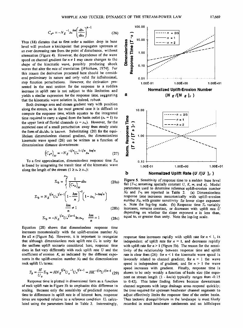
Figure 5. Sensitivity of response time to a sudden base level fall (T,•,; assuming spatially constant U, K, m, and n). Model parameters used to determine reference uplift-erosion number NL- and T,b are reported in Table 2. (a) Dimensionless response time increases monotonically with uplift-erosion number NE, with greater sensitivity for lower slope exponent n. Note the log-log scale. (b) Response time Tb variably increases, remains constant, or decreases with uplift rate U depending on whether the slope exponent n is less than, equal to, or greater than unity. Note the log-log scale.

Equation (28) shows that dimensionless response time increases monotonically with the uplift-erosion number NE for all n (Figure 5a). However, it is important to recognize that although dimensionless rock uplift rate U, is unity for the uniform uplift scenario considered here, response time does in fact vary differently with rock uplift rate U and the coefficient of erosion K, as indicated by the different exponents in the uplift-erosion number Ne and the dimensionless rock uplift U, terms:

Tb = H T*b • mNœ1/nWo -1w*l/n-1 • mK-1/nwl/n-1 (29) Uo

Response time is plotted in dimensional form as a function of rock uplift rate in Figure 5b to emphasize this difference in scaling. Because only the sensitivity of predicted response time to differences in uplift rate is of interest here, response times are reported relative to a reference condition Ur calculated using the parameters listed in Table 2. Interestingly,

response time increases rapidly with uplift rate for n < 1, is independent of uplift rate for n = 1, and decreases rapidly with uplift rate for n > 1 (Figure 5b). The reason for the sensitivity of the relationship between response time and uplift rate is clear fi'om (26): for n < 1 the kinematic wave speed is inversely related to channel gradient; for n = 1 the wave speed is independent of gradient; and for n > 1 the wave speed increases with gradient. Finally, response time is shown to be only weakly a function of basin size (the exponent on stream length (1 - hrn/n) typically ranges from -0.15 to 0.42). This latter finding follows because downstream channel segments with large drainage areas respond quickly; the time required for upstream headwater channel segments to adjust effectively limits the response time of the entire basin. Thus tectonic disequilibrium in the landscape is most likely recorded in small headwater catchments and on hillslopes


that have not yet responded to rapid adjustments of the channel system. Further, a field-testable prediction of this model is the location of knickpoints correlated with known (coseismic or eustatic) base level drops [e.g., see Rosenbloom and Anderson, 1994].

5.2. Sudden Increase in Uplift Rate

Response time for a step function increase in uplift rate Tt• is derived in a different manner. Application of the kinematic wave solution is not straightforward in this case because this problem entails a significant deviation from the base steady state and because the channel is subjected to a sustained rate of base level fall, rather than a discrete perturbation. In fact, the derivation presented here is more robust than the kinematic wave solution above as it is not subject to any uncertainties related to knickpoint shape evolution during upstream migration.

An increase in uplift rate initiates a wave of erosion that propagates upstream (Figure 6). Equilibrium within the fluvial system is reached when the wave of erosion reaches the fluvial channel tips (x = Xc), as argued above. We reason that arrival of this migrating knickzone at the fluvial channel tips coincides with the time that they attain their final elevation (ZAXc)). In other words, the migrating knickzone defines the boundary between a downstream segment of the profile that has achieved its final equilibrium gradient and an upstream segment that has not yet steepened in response to the change in rock uplift rate. Barring the effects of numerical diffusion, this is precisely the behavior observed in numerical solutions of the profile evolution equation (18). Thus response time is set by the time required to elevate the fluvial channel tips from an initial equilibrium position (zi(xc)) to a final equilibrium position (Figure 6):

(xc)- + (30)

4

z t (x c ) '•• final steady state profile E

• dz/dt =Uf '•i =Uf -Ui o

• of erosion

z,(xc) •,.j .•..•..œ, • 0 5 10 15 20 25

Distance from Divide (kin)

Figure 6. Schematic illustration of the transient response (solid line) of an equilibrium channel (shaded line) to a sudden increase in rock uplift rate used in the derivation of response timescale Ts. Rock uplffi rates •e indicated by solid arrows; headwater erosion rates •e indicated by shaded arrows. An increase in uplffi rate instigates a wave of erosion that propagates upstream. Channel headwater reaches •e uplffied but do not respond until the wave of erosion reaches them. Accordingly, z(xO increases at a constant rate (dz/dt = U•- UO until a new equilibrium is reached (dashed shaded line).

Since the upper reach of the fluvial channel does not respond to the change in uplift rate until the wave of erosion reaches this point, from (11) the time rate of change of the elevation of the fluvial channel tips Z(Xc) is given by the difference between the newly imposed uplift rate Uf and the previ- ously established erosion rate (ci(Xc)):

Rearranging and noting that for perturbation away from an initial steady state the erosion rate at the fluvial channel tips is equal to the initial uplift rate (c•(Xc)= UO, we obtain the simple result:

Tu = U f - U i (32) Using (32), the system response timescale can be directly

estimated from field observations, provided certain restrictive conditions are met: (1) adjacent terranes of similar climate and lithology are experiencing different, known rock uplift rates, and (2) channel profiles appear to have adjusted to imposed uplift rates; profiles have smooth logarithmic forms with no indication of an active, propagating knickzone [Snyder and Whipple, 1998; Snyder et al., submitted manuscript, 1999]. These conditions will rarely be met, however, and it is useful to write (32) in terms of nondimensional rock uplift rate, system length, and rock erosion parameters, using (24) for dimensionless timescale:

U,f(]_$) (33a) Si

•f=f (33b) where Uo/is chosen as the reference rock uplift rate.

Using (21) to determine z,i(X,c) and z,•(X,c), substituting into (33), and rearranging gives an algebraic relationship for dimensionless response timescale T,t•:

E ta,f 1- hrn/ n

• 1 (34a) n

ß r 1/nrr l/n-1 (1 -" E •'*f lnx, c _ fl/n) hm = --= 1 (34b) T*u (l-f) n

Note that for the case of uniform rock uplift rate treated here the dimensionless uplift rate term U,/is unity. As in the derivation of Tb, we have assumed block uplift (dU/dx = O) and spatially uniform coefficient of erosion and erosion process (dK/dx = 0; n and m are constants). For Ui = 0 the initial condition is a horizontal plane, and the erosion rate at the fluvial channel headwater is zero until the wave of erosion

has swept through the entire fluvial system. In this case the response time is simply the quotient of the equilibrium elevation above the base level of the channel at x = Xc and the

uplift rate Uo/. Interestingly, (34) reduces to the kinematic wave solution (equation (28)) in this case (Ui = 0; f= 0). In other words, it takes as long for a discrete base level fall to be


10

Fixed Final Uplift Rate (U f )

E

o

a

0.1

0.01

....... n = 2/3

•n=l

.... n=2

i i i i i iiI I i i i i i i •1

0.1

Uplift Rate Ratio (f =U / IU f )

lO

Fixed Initial Uplift Rate (U • )

_

0.1

0.01

2/3

•n=l

-

i i i , i i ii I i i i i i i i i

0.1

Uplift Rate Ratio (f =U / I U f )

Figure 7. Timescale of response to a step function increase in uplift rate (Tu; assuming spatially constant U, K, m, and n). Reference values of rock uplift rate Ur and the response timescale Tur used to normalize the plots are given by or derived from parameter values reported in Table 2. Note that if the initial uplift rate is zero (Ui = 0), the response time is given by the base level fall solution (Figure 5). (a) Sensitivity of response time to the magnitude of the increase in uplift rate (UdUf) for the case where the final uplift rate Uf is held constant. Response time increases with U• (increasing UdUf) for n < 1, is independent of Ui for n = 1, and decreases with U• for n > 1. (b) Sensitivity of response time to the magnitude of the increase in uplift rate (UdUf) for the case where the initial uplift rate U• is held ccnstant. Response time increases with Uf (decreasing UdUf) for n < 1, is independent of Uf for n =1, and decreases with Uf for n > 1.

than with the coefficient of erosion K. For this reason, response time is plotted in dimensional form as a function of the rock uplift rate relative to a reference condition (Figure 7). Additionally, the appearance of both initial and final rock uplift rates in both the numerator and the denominator (through fand NE) indicates that there is an additional level of complexity in the dependence of response time on rock uplift rates. Accordingly, Figure 7a is plotted to illustrate the relationship between response time and final uplift rate Uf and Figure 7b illustrates the relationship between response time and initial uplift rate Ui.

Some nonintuitive effects are revealed in the relationship between the magnitude of the change in uplift rate and response time (Figure 7). As seen in the case of a sudden base level fall, for n = 1, response time is independent of both the final uplift rate Uf and the magnitude of the change in uplift rate (Figures 7a and 7b). Interestingly, for the case n > 1, system response time decreases for smaller changes in uplift rate (i.e., as UdUf approaches 1) where Uf is held constant (Figure 7a) but actually increases for smaller changes in uplift rate where U• is held constant (Figure 7b). Conversely, for the case of n < 1, response time increases for smaller changes in uplift rate where Uf is held constant (equation (34); Figure 7a) and decreases for smaller changes in uplift rate where U• is held constant (equation (34); Figure 7b). This yields the seemingly odd result that for n < 1 it takes significantly longer to adjust to a minor change in uplift rate than it does to raise the entire range starting from a horizontal plane. The reason for this is twofold: (1) the relationship between uplift rate and equilibrium channel headwater elevation is nonlinear in the slope exponent n (equation (21)), and (2) the rate at which the channel headwater is elevated depends on the initial slope at x = Xc.

Simplifying (34) and writing it in dimensional form, we see that the change in channel headwater elevation required with an increase in uplift rate scales as

while the rate of change of channel headwater elevation scales with the difference between final and initial rock uplift rates'

dt oc U f - U i (36) This finding has important implications for the differing dynamic response of landscapes (both real and simulated) etched by different sets of erosional processes (e.g., abrasion by suspended load, abrasion by saltation load, and plucking), through their control of the slope exponent n.

translated the length of a channel system at equilibrium with the prevailing uplift rate as it would to uplift the entire range from base level, a somewhat surprising result with potentially interesting field applications.

Equation (34) reveals a rather complex relationship between the system response timescale, the initial conditions, and the dominant erosion processes that govern the slope exponent n. As with the response time to sudden base level fall, because T,s is normalized by average uplift rate Uof, the actual response time scales differently with uplift rate U

6. Conclusions: Research Needs and Approaches

Review of the underlying assumptions and approxima- tions of the shear-stress/stream-power erosion model, consideration of steady state river profiles, and exploration of the controls on bedrock channel response times establish in no uncertain terms that resolving questions regarding the nonlinearity of the dominant bedrock erosion process(es) are paramount to further fundamental progress in understanding landscape response to tectonic and climatic change. Dimen- sional analysis demonstrates that a single nondimensional


group, here termed the uplift-erosion number, encapsulates the dependence of predicted erosion rates on tectonic, lithologic, and climatic variables. Our sensitivity analysis of the dimensionless river profile evolution equation (18) reveals that both the magnitude and timescale of the bedrock channel response to an imposed tectonic or climatic forcing are largely governed by the uplift-erosion number raised to a power determined by the slope exponent n in the stream- power erosion law (equation (1)). Also, the much discussed m/n ratio is shown to influence significantly the shape (and thereby response timescale)of river profiles. However, the m/n ratio neither influences the sensitivity of channel gradient, relief, or response timescale to changes in the uplift- erosion number nor the dependence of this sensitivity on the slope exponent n. Furthermore, for the broad subset of fluvial erosion processes adequately described by (2)- (7)the m/n ratio is shown to be restricted to a narrow range (0.35 - 0.6).

The slope exponent n, which emerges from the analysis as a critical unknown, has been shown above to be directly related to the degree of nonlinearity in the relationship between erosion rate and shear stress (or stream power). Thus the dominant fluvial erosion processes directly and pro- foundly influence the dynamic behavior of fluvial bedrock stream channels. Clearly, it is not satisfactory simply to assume that erosion is linearly related to shear stress (or stream power); the relationship between channel gradient and erosion rate and its potential variation between field set- tings are first-order problems in tectonic geomorphology.

As the slope exponent n is directly related to the physics of the active erosion processes, directed small-scale field and modeling studies of these processes are greatly needed. Potential erosion processes include plucking, bashing by bedload, abrasion by suspended load, cavitation, solution, and weathering [Alexander, 1932; Maxson and Campbell, 1935; Barnes, 1956; Foley, 1980; Wohl, 1993; Zen and Prestegaard, 1994; Hancock et al., 1998; Sklar and Dietrich, 1998; Whipple et al., submitted manuscript, 1999]. A number of field and laboratory studies are underway [e.g., Slingerland et al., 1997; Sklar and Dietrich, 1998; Snyder and Whipple, 1998; Snyder et al., submitted manuscript, 1999], but many questions remain unanswered.

Study of the variation in the effective erosion coefficient K accompanying adjustments to imposed boundary conditions is also greatly needed. In most modeling studies to date, including our analysis presented above, the coefficient of erosion has been treated as a constant (dK/dt = 0; dK/dx = 0). In addition to the obvious assumption that lithology and precipitation be held constant in space and time, holding K constant carries the implicit assumption that slope is the only morphologic variable that may adjust in response to a change in boundary conditions. Even in the simplest cases, this assumption will often be violated, with either the amount of alluvial/colluvial cover [e.g., Howard, 1998; Sklar and Dietrich, 1998] or the channel width changing in concert with the gradient. Spatial and temporal variations in the coefficient of erosion may importantly influence the dynamics of river response to tectonic and climatic forcing.

The classic problem of scaling observations of local erosion rates and processes up to the reach scale relevant in landscape evolution models is, of course, a difficulty faced by small-scale process studies. A major hurdle in this effort will be finding an effective way to constrain the reach-averaged competition and interaction of the various erosion processes active at the bed. Answers to several questions are needed.

Which process is dominant under what conditions? What are the appropriate forms of (2) and (3)? Over what distance is an appropriate gradient measured? Similarly, the need to integrate over the full spectrum of flood discharges to derive a meaningful long-term average rate is a problem [Willgoose, 1989; Tucker and Bras, 1997]. One approach that may help to bridge this gap is to pursue small-scale process-oriented field studies in conjunction with reach-scale modeling studies, pursuing top-down and bottom-up approaches in concert. Field areas encompassing known differences in either climate, lithology, or uplift histories but similar in other respects will be critical to such studies [e.g., Merritts and Vincent, 1989; Snyder and Whipple, 1998; Snyder et al., submitted manuscript, 1999]. Moreover, field areas where a transient response to a recent climatic or tectonic perturbation from a known initial condition can be studied would be

most advantageous because o? the sensitivity of predicted transient responses to critical model parameters.

Notation

Variables

re

f(qs) f g

H

L

Q

R•c s

Sc

t

v

w

x

Xc

vertical erosion rate [LT-•]. density of water [ML -3]. basal shear stress [ML '•T'2]. upstream drainage area [L 2]. critical upstream drainage area for fluvial erosion processes [L 2]. kinematic wave speed [LT'•]. hydraulic friction factor. average flow depth [L]. erodibility scaling factor for sediment loading. rock uplift rate ratio. gravitational acceleration [LT'2]. representative vertical length scale [L]. total bedrock stream length [L]. discharge [L 3T-•]. fluvial bedrock channel relief [L]. hillslope and colluvial channel relief [L]. streamwise channel bed gradient. average gradient of hillslope/colluvial channel profile. time [7]. response time for sudden baselevel fall [7]. response time for step increase in uplift rate [T]. rock uplift rate defined relative to erosional base level [LT4]. average rock uplift rate defined relative to erosional base level [LT-•]. mean velocity [LT'•]. channel width [L]. streamwise distance from divide [L]. critical distance for transition to fluvial erosion [L]. elevation of stream bed [L].

Exponents a shear-stress or stream-power exponent. b exponent in channel width-discharge relation. c exponent in discharge-area relation. h exponent in area-length relation (reciprocal

Hack's exponent). area exponent, erosion rule. slope exponent, erosion rule.


Dimensional constants

K coefficient of erosion [L •-2m ka area-length coefficient [L 2-h]. kb total erodibility [M-•L a+lr2a-1 (shear-stress) or M

LT 3a-i (stream-power)]. ke intrinsic erodibility [M-aL a+lT 2a-i (shear-stress) or

M -• LT 3a-1 (stream-power)]. kq discharge-area coefficient (effective precipitation)

[L 3-2½ T-l]. channel width-discharge coefficient [L •-3b T •].

Dimensionless variables

re,

NEr

R,f S,

t,

T,•

r,u

X*c

dimensionless kinematic wave speed. uplift-erosion number. reference value of the uplift-erosion number. dimensionless fluvial bedrock channel relief.

dimensionless channel gradient. dimensionless time.

dimensionless response time for sudden base level fall.

dimensionless response time for step increase in uplift rate. dimensionless rock uplift rate. dimensionless distance downstream.

dimensionless critical distance for transition to fluvial erosion.

dimensionless streambed elevation.

Acknowledgments. Funding for this research was provided by NSF grants EAR-9614970 and EAR-9725723 with additional support from the Army Construction Engineering Research Lab (DACA-88--95-R- 0020). We thank R. Anderson and G. Hancock for stimulating discus- sions of bedrock channel processes in the field and J. Pelletier for a discussion of controls on the concavity index (hm/n). N. Snyder and E. Kirby provided the data reported in Table 1. This paper benefited greatly from critical reviews by W. Dietrich, A. Howard, and L. Sender.

References

Adams, J., Large-scale tectonic geemorphology of the Southern Alps, New Zealand, in Tectonic Geemorphology, edited by M. Morisawa and J.T. Hack, pp. 105-128, Allen and Unwin, Winchester, Mass., 1985.

Alexander, H.S., Pothole erosion, J. Geol., 40, 307-335, 1932. Anderson, R.S., The growth and decay of the Santa Cruz Mountains, J.

Geephys. Res., 99, 20,161-20,180, 1994. Barnes, H.L., Cavitation as a geological agent, Am. J. Sci., 254, 493-

505, 1956. Beaumont, C., P. Fullsack, and J. Hamilton, Erosional control of active

compressional oregens, in Thrust Tectonics, edited by K.R. McClay, pp. 1-18, Chapman and Hall, New York, 1992.

Bird, P., Lateral extrusion of lower crust from under high topography, in the isostatic limit, J. Geephys. Res., 96, 10,275-10,286, 1991.

Dietrich, W.E., D. Allen, D. Bellugi, M. Trso, and L. Sklar, Digital ter- rain analysis of bedrock channel incision, in Bedrock Channel Con- ference, edited by E.E. Wohl and K. Tinkler, pp. 22, Colorado State Univ., Fort Collins, 1996.

Fernandes, N.F., and W.E. Dietrich, Hillslope evolution by diffusive processes: the timescale for equilibrium adjustments, Water Resour. Res., 33, 1307-1318, 1997.

'Fielding, E.J., B.L. Isacks, M. Barazangi, and C. Duncan, How flat is Tibet?, Geology, 22, 163-167, 1994.

Flint, J.J., Stream gradient as a function of order, magnitude, and discharge, Water Resour. Res., 10, 969-973, 1974.

Foley, M.G., Bed-rock incision by streams, Geol. Sec. Am. Bulletin, Part 2, 91, 2189-2213, 1980.

Goldrick, G., and P. Bishop, Stream long profile analyses and the reconstruction of landscape evolution with examples from the Lachlan Valley, southeastern Australia, in Bedrock Channel Con-

ference, edited by E.E. Wohl and K. Tinkler, pp. 23, Colorado State Univ., Fort Collins, 1996.

Hack, J.T., Studies of longitudinal stream profiles in Virginia and Maryland, U.S. Geol. Surv. Prof. Pap., 294-B, 97, 1957.

Hack, J.T., Stream profile analysis and stream-gradient index, J. Res. U.S. Geol. Surv., 1,421-429, 1973.

Hancock, G.S., R.S. Anderson, and K.X. Whipple, Beyond power: Bedrock river incision process and form, in Rivers Over Rock: Fluvial Processes in Bedrock Channels, Geephys. Monogr. Set., vol. 107, edited by K. Tinkler and E.E. Wohl, pp. 35-60, AGU, Washington, D.C., 1998.

Hovius, N., C.P. Stark, H.T. Chu, and J.C. Lin, Supply and removal of sediment in a landslide-dominated mountain belt: Central Range, Taiwan, J. Geol., in press, 1999.

Howard, A.D., A detachment-limited model of drainage basin evolution, Water Resour. Res., 30, 2261-2285, 1994.

Howard, A.D., Badland morphology and evolution: Interpretation using a simulation model, Earth Surf. Processes Landforms, 22, 211-227, 1997.

Howard, A.D., Long profile development of bedrock channels: Inter- action of weathering, mass wasting, bed erosion, and sediment transport, in Rivers Over Rock: Fluvial Processes in Bedrock Channels, Geephys. Monogr. Set. vol. 107, edited by K. Tinkler and E.E. Wohl, pp. 297-319, AGU, Washington, D.C., 1998.

Howard, A.D., and G. Kerby, Channel changes in badlands, Geol. Sec. Am. Bulletin, 94, 739-752, 1983.

Howard, A.D., M.A. Seidl, and W.E. Dietrich, Modeling fluvial erosion on regional to continental scales, J. Geephys. Res., 99, 13,971- 13,986, 1994.

Humphrey, N.F., and P.L. Heller, Natural oscillations in coupled geomorphic systems: An alternative origin for cyclic sedimentation, Geology, 23, 499-502, 1995.

Isacks, B.L., 'Long-term' land surface processes: Erosion, tectonics and climate hietnry in mn,,ntaln holte in T ....t. Understanding ,t.• Ter- restrial Environment, edited by P.M. Mather, pp. 21-36, Taylor and Francis, Bristol, Pa., 1992.

Kooi, H., and C. Beaumont, Escarpment evolution on high-elevation rif•ed margins: Insights derived from a surface processes model that combines diffusion, advection, and reaction, d. Geephys. Res., 99, 12,191-12,209, 1994.

Keens, P.O., The topographic evolution of collisional mountain belts: a numerical look at the Southern Alps, New Zealand, Am. d. Sci., 289, 1041-1069, 1989.

Leopold, L.B., and T. Maddock, The hydraulic geometry of stream channels and some physiographic implications, U.S. Geol. Surv. Prof. Pap., 252, 1953.

Maritan, A., A. Rinaldo, R. Rigon, A. Giacometti, and I. Rodriguez- Itrube, Scaling laws for river networks, Phys. Rev. E., Stat. Phys. Plasmas Fluids Relat. Interdiscip. Top., 53, 1510-1515, 1996.

Masek, J.G., B.L. Isacks, and E.J. Fielding, Rit• flank uplit• in Tibet: Evidence for a viscous lower crust, Tectonics, 13, 659-667, 1994a.

Masek, J.G., B.L. Isacks, T.L. Gubbels, and E.J. Fielding, Erosion and tectonics at the margins of continental plateaus, J. Geephys. Res., 99, 13,941-13,956, 1994b.

Maxson, J.H., and I. Campbell, Stream fluting and stream erosion, J. Geol., 43, 729-744, 1935.

Merritts, D., and K.R. Vincent, Geomorphic response of coastal streams to low, intermediate, and high rates of uplift, Mendocino junction region, northern California, Geol. Sec. Am. Bulletin, 101, 1373-1388, 1989.

Moglen, G.E., and R.L. Bras, The effect of spatial heterogeneities on geomorphic expression in a model of basin evolution, Water Resour. Res., 31, 2613-2623, 1995a.

Moglen, G.E., and R.L. Bras, The importance of spatially heterogene- ous erosivity and the cumulative area distribution within a basin evolution model, Geemorphology, 12, 173-185, 1995b.

Molnar, P., and P. England, Late Cenozoic uplitt of mountain ranges and global climate change: Chicken or egg?, Nature, 346, 29-34, 1990.

Molnar, P., and H. Lyon-Caen, Some simple physical aspects of the support, structure, and evolution of mountain belts, Geol. Sec. Am. Spec. Pap., 218, 179-207, 1988.

Montgomery, D.R., and E. Foufoula-Georgiou, Channel network repre- sentation using digital elevation models, Water Resour. Res., 29, 1178-1191, 1993.

Montgomery, D.R., T.B. Abbe, J.M. Buffington, N.P. Peterso'n, K.M. Schmidt, and J.D. Stock, Distribution of bedrock and alluvial chan-


nels in forested mountain drainage basins, Nature, 381, 587-589, 1996.

Raymo, M.E., and W.F. Ruddiman, Tectonic forcing of late Cenozoic climate, Nature, 359, 117-122, 1992.

Rigon, R., I. Rodriguez-Iturbe, A. Maritan, A. Giacometti, D. Tarboton, and A. Rinaldo, On Hack's law, Water Resour. Res., 32, 3367-3374, 1996.

Rosenbloom, N.A., and R.S. Anderson, Evolution of the marine ter- raced landscape, Santa Cruz, California, d. Geophys. Res., 99, 14,013-14,030, 1994.

Schmidt, K.M., and D.R. Montgomery, Limits to relief, Science, 270, 617-620, 1995.

Schumm, S.A., Geomorphic thresholds: The concept and its applications, Trans. Inst. Br. Geogr., NS 4, 485-515, 1979.

Schumm, S.A., and R.S. Parker, Implications of complex response of drainage systems for Quaternary alluvial stratigraphy, Nature Phys. Sci., 243, 99-100, 1973.

Seidl, M.A., and W.E. Dietrich, The problem of channel erosion into bedrock, Catena Suppl., 23, 101-124, 1992.

Seidl, M., W.E. Dietrich, and J.W. Kirchner, Longitudinal profile development into bedrock: An analysis of Hawaiian channels, d. Geol., 102, 457-474, 1994.

Seidl, M.A., J.K. Weissel, and L.F. Pratson, The kinematics of escarpment retreat across the rifted continental margin of SE Australia, Basin Res., 12, 301-316• 1996.

Sklar, L., and W.E. Dietrich, The influence of downstream variations in sediment supply and transport capacity on bedrock channel longitudinal profiles, Eos Trans. AGU, 78 (46), Fall Meet. Suppl. F299, 1997.

Sklar, L., and W.E. Dietrich, River longitudinal profiles and bedrock incision models: Stream power and the influence of sediment supply, in Rivers Over Rock: Fluvial Processes in Bedrock Channels, Geosphys. Monogr. Ser., vol. 107, edited by K.J. Tinkler and E.E. Wohl, pp. 237-260, AGU, Washington, D.C., 1998.

Slingerland, R., S.D. Willet, and H.L. Hennessey, A new fluvial bedrock erosion model based on the work-energy principle, Eos Trans. AGU, 78 (46), Fall Meet. Suppl. F299, 1997.

Slingerland, R., S.D. Willett, and N. Hovius, Slope-area scaling as a test of fluvial bedrock erosion laws, Eos Trans. AGU, 79 (45), Fall Meet. Suppl. F358, 1998.

Snyder, N.P., and K.X. Whipple, New constraints on bedrock channel response to varying uplift, King Range, California, paper presented at Annual Conference, Am. Assoc. Pet. Geol. /Soc. Sediment. Geol., Salt Lake City, 1998.

Stock, J.D., Can we predict the rate of bedrock river incision using the stream power law?, M.S. thesis, Univ. of Wash., Seattle, 1996.

Stock, J.D., and D.R. Montgomery, Geologic constraints on bedrock river incision using the stream power law, J. Geophys. Res., 104, 4983-4993, 1999.

Suzuki, T., Rate of lateral planation by Iwaki River, Japan, Trans. Jpn. Geomorphol. Union, 3, 1-24, 1982.

Tarboton, D.G., R.L. Bras, and I. Rodriguez-Iturbe, Scaling and elevation in river networks, Water Resour. Res., 25, 2037-2051, 1989.

Tarboton, D.G., R.L. Bras, and I. Rodriguez-Iturbe, On the extraction of channel networks from digital elevation data, Hydrol. Proc., 5, 81-100, 1991.

Tucker, G.E., Modeling the Large-Scale Interaction of Climate, Tec- tonics and Topography, Pa. State Univ. Earth Syst. Sci. Cent., Uni- versity Park, 1996.

Tucker, G.E., and R.L. Bras, The role of rainfall variability in drainage basin evolution: Implications of a stochastic model, Eos Trans. AGU, 78 (46), Fall Meet. Suppl., F282, 1997.

Tucker, G.E., and R.L. Bras, Hillslope processes, drainage density, and landscape morphology, Water Resour. Res., 34, 2751-2764, 1998.

Tucker, G.E., and R. Slingerland, Predicting sediment flux from fold and thrust belts, Basin Res., 8, 329-349, 1996.

Tucker, G.E., and R.L. Slingerland, Drainage basin response to climate change, Water Resour. Res., 33, 2031-2047, 1997.

Whitham, G.B., Linear and Non-Linear Waves, 636 pp., John Wiley, New York, 1974.

Willgoose, G., A physically based channel network and catchment evolution model, Ph.D. thesis, Mass. Inst. of Technol., Cambridge, 1989.

Willgoose, G., A physical explanation for an observed area-slope-elevation relationship for catchments with declining relief, Water Resour. Res., 30, 151-159, 1994.

Willgoose, G., R.L. Bras, and I. Rodriguez-Iturbe, A model of river basin evolution, Eos Trans. AGU, 71, 1806-1807, 1990.

Willgoose, G., R.L. Bras, and I. Radriguez-Iturbe, A coupled channel network growth and hillslope evolution model. 2. Nondimensionali- zation and applications, Water Resour. Res., 27, 1685-1696, 1991.

Wahl, E.E., Bedrock channel incision along Picanniny Creek, Australia, d. Geol., 101,749-761, 1993.

Wahl, E.E., N. Greenbaum, A.P. Schick, and V.R. Baker, Controls on bedrock channel incision along Nahal Paran, Israel, Earth Surf. Processes Landforms, 19, 1-13, 1994.

Wolman, M.G., and J.P. Miller, Magnitude and frequency of forces in geomorphic processes, d. Geol., 68, 54-74, 1960.

Zen, E.-A., and K.L. Prestegaard, Possible hydraulic significance of two kinds of potholes: Examples from the paleo-Potomac River, Geology, 22, 47-50, 1994.

G. E. Tucker, Department of Civil and Environmental Engineering, Massachusetts Institute of Technology, Cambridge, MA 02139.

K. X. Whipple, Department of Earth, Atmospheric and Planetary Sciences, Massachusetts Institute of Technology, Cambridge, MA 02139. (kxw@mit. edu)

(Received March 6, 1998; revised March 5, 1999; accepted March 19, 1999.)

dynamics of the stream-power river incision model...

Documents