dynamics of shape memory alloy coated micro … and dynamical behavior of shape memory alloy coated...
TRANSCRIPT
Dynamics of ShapeMemory Alloy coated
micro cantilevers- theory and experiments -
Thijs Kniknie
DCT 2008.085
Master Thesis
SupervisorsProf. Dr. Henk NijmeijerDynamics & ControlDr. Yves BellouardMicro & NanoScale Engineering
Eindhoven University of TechnologyDepartment of Mechanical Engineering
Eindhoven, July 2nd, 2008

Preface
This project is the result of a collaboration between the groups Dynamics & Control andMicro & NanoScale Engineering. The experience of both groups about dynamics, modeling,materials science and experimental techniques is combined, in order to investigate thethermomechanical and dynamical behavior of Shape Memory Alloy coated micro cantilevers.The results give way to research on micro vibration control and future joint projects of thesegroups.
During this research, the help of experts from various fields of work was of great value. Iwant to thank Marc van Maris of the Mechanics of Materials group for the opportunity touse the equipment in the Multi-scale laboratory. From the Micro & NanoScale Engineeringgroup, I thank Willie ter Elst for helping with the realization of the experimental setup, aswell as Eric Homburg, for giving advice about the optics and electronics.
I greatly appreciate the effort of dr. Xi Wang of Harvard University for sputter coatingand annealing the NiTi thin films on our micro cantilever samples. With these excellentsamples, we were able to do several unique and interesting thermomechanical and dynamicalexperiments. I am also very thankful of Michael Hopper (formerly working at QuintenzHybridtechnik) who designed in his spare time the piezoelectric amplifier electronic circuit.
I thank prof. dr. Henk Nijmeijer for our inspiring discussions during the project. Last, butnot least, I thank dr. Yves Bellouard for his personal coaching on every aspect of the project.I could walk by almost anytime and I could always expect an enthusiastic reaction on myresults.

Abstract
With the increasing attention for the use of Micro Electro Mechanical Systems (MEMS) invarious fields of work, gaining knowledge about the dynamics of these devices is an interestingnew research topic. In this project, a structural solution for actively influencing the dynamicsof a micro cantilever, using a Shape Memory Alloy (SMA) coating, is investigated. AnSMA shows temperature- and stress-induced martensitic phase transformations, drasticallychanging the material’s mechanical properties and adding damping. The influence of thischange on the thermomechanical and dynamical behavior of the cantilever is experimentallyand theoretically analyzed.
Samples of commercially available Silicon micro cantilevers are sputter-coated withequiatomic Nickel-Titanium (NiTi). To investigate the thermomechanical behavior of thecoated cantilevers, temperature-stress curves are experimentally obtained. The curvesclearly show two-step hysteretic phase transformations between Martensite, R-Phase andAustenite. Several material properties can be deduced from the slope of the curves. Athermomechanical model is formulated, describing the stress evolution in the interface layerbetween the film and substrate as function of temperature. The stress is decomposed intobimorphic stress and phase transformation stress. For modeling the phase transformationstress, several mathematical models are discussed. Eventually the Krasnosel’skii-Pokrovskiihysteron is chosen because of its appealing simplicity, while still capable of capturing mostof the geometrical properties of the hysteresis curve.
An experimental setup is designed, capable of exciting the micro cantilevers to highfrequencies, simultaneously heating them and measuring their dynamic response. The resultsshow that the flexural resonance frequency of the beam for increasing temperature firstdecreases due to a change of the geometry of the cross-section. Upon further increasingthe temperature, the phase transition results in an increase of the resonance frequency upto 10%. Near the flexural resonance, a second resonance frequency is seen, only slightlychanging as function of temperature. The two modes separate or merge for increasingtemperature. These observations make it difficult to assess damping, but pose an interestingnew research topic. A model of the structural dynamic of the cantilevers is made, includingthe temperature dependence of the resonance frequencies. The numerical results partiallycorrespond with with the measurements.
The results show that with an SMA coating it is possible to actively influence the dynamicsof the cantilevers. Further research has to show whether the influence is sufficient for usefulapplications in MEMS.

Samenvatting
In de afgelopen decennia is de interesse in het gebruik van Micro Electro-MechanischeSystemen (MEMS) toegenomen. Het analyseren van het dynamisch gedrag van dezesystemen is daarbij een nieuw onderzoeksgebied. In dit project is een structurele oplossingvoor het actief aanpassen van het dynamisch gedrag van een eenzijdig ingeklemde microbalk onderzocht, door middel van het aanbrengen van een film van geheugenmetaal. Onderinvloed van temperatuur en spanning vertoont geheugenmetaal drastische veranderingenin materiaaleigenschappen. De invloed hiervan op het thermomechanische en dynamischegedrag van de balk is experimenteel en theoretisch onderzocht.
Commercieel verkrijgbare Silicium micro balken zijn met een dunne film Nikkel-Titanium(NiTi) gecoat door sputterdepositie. Het thermomechanische gedrag van deze balkenis beoordeeld door de temperatuur-spanningscurves te meten. Er is een tweetrapsfasetransformatie zichtbaar tussen de Martensiet fase, R-fase en Austeniet fase. Verschillendemateriaalparameters kunnen vervolgens bepaald worden met behulp van deze grafieken.Een thermomechanisch model is geformuleerd, dat het spanningsverloop in de filmbij de aanhechting met de balk beschrijft. De spanning is daartoe opgedeeld infasetransformatie spanning en in spanning die veroorzaakt is door een verschil in dethermische expansiecoefficienten. Voor het beschrijven van de fasetransformatie spanningwordt een aantal modellen besproken. Het Krasnosel’skii-Pokrovskii hysteron wordtuiteindelijk gekozen vanwege haar eenvoud, terwijl het model tevens de belangrijksteeigenschappen van de hysterese lus beschrijft.
Er is een experimentele opstelling ontworpen, waarmee het mogelijk is de balken teexciteren, op te warmen en de dynamische responsie te meten. De resultaten laten ziendat de eigenfrequentie voor buiging bij stijgende temperatuur lichtelijk afneemt, om nafasetransformatie tot 10% toe te nemen. Rond deze buigresonantie is een tweede resonantiete zien, welke licht verandert als functie van de temperatuur. Deze resonanties vallen samenof scheiden zich bij stijgende temperatuur. Dit gegeven bemoeilijkt het onderzoeken van dedempingseigenschappen van het materiaal, maar levert daarentegen nieuwe onderzoeksvragenop. Een model van de structurele dynamica van de balken is geformuleerd, waarin de deresonantiefrequenties afhankelijk zijn van de temperatuur. Deze numerieke simulaties wordenvergeleken met de gemeten responsies.
De resultaten laten zien dat het mogelijk is met een SMA coating het dynamisch gedrag vande balken te beınvloeden. Aanvullend onderzoek is nodig om te onderzoeken of de invloedvan dit de fasetransformaties voldoende is voor concrete toepassingen in MEMS.

Contents
Preface i
Abstract iii
Samenvatting v
Contents vii
1 Introduction 1
1.1 Applications of micro cantilevers . . . . . . . . . . . . . . . . . . . . . . . . . 2
1.2 Shape Memory Alloys . . . . . . . . . . . . . . . . . . . . . . . . . . . . . . . 4
1.3 Problem definition . . . . . . . . . . . . . . . . . . . . . . . . . . . . . . . . . 6
2 Experimental setup 9
2.1 Specifications . . . . . . . . . . . . . . . . . . . . . . . . . . . . . . . . . . . . 9
2.2 Experimental setup design . . . . . . . . . . . . . . . . . . . . . . . . . . . . . 11
2.2.1 Sample preparation . . . . . . . . . . . . . . . . . . . . . . . . . . . . 12
2.2.2 Excitation stage . . . . . . . . . . . . . . . . . . . . . . . . . . . . . . 13
2.2.3 Measurement stage . . . . . . . . . . . . . . . . . . . . . . . . . . . . . 15
2.2.4 Heating . . . . . . . . . . . . . . . . . . . . . . . . . . . . . . . . . . . 18
2.2.5 Assembly . . . . . . . . . . . . . . . . . . . . . . . . . . . . . . . . . . 19
2.3 Characterization of the experimental setup . . . . . . . . . . . . . . . . . . . 21
3 Modeling of the coated cantilever 27
3.1 Thermomechanics . . . . . . . . . . . . . . . . . . . . . . . . . . . . . . . . . 28
3.2 Transformation stress – hysteresis modeling . . . . . . . . . . . . . . . . . . . 32
3.2.1 Hysteresis models . . . . . . . . . . . . . . . . . . . . . . . . . . . . . . 32
3.2.2 Preisach model . . . . . . . . . . . . . . . . . . . . . . . . . . . . . . . 35
3.2.3 Duhem model . . . . . . . . . . . . . . . . . . . . . . . . . . . . . . . . 37
3.2.4 Krasnosel’skii-Pokrovskii hysteron . . . . . . . . . . . . . . . . . . . . 40
3.3 Dynamics of cantilever beams . . . . . . . . . . . . . . . . . . . . . . . . . . . 42
3.4 Heat transfer . . . . . . . . . . . . . . . . . . . . . . . . . . . . . . . . . . . . 44
4 Experiments and simulations 49
4.1 Thermomechanics . . . . . . . . . . . . . . . . . . . . . . . . . . . . . . . . . 50
4.2 Joule heating . . . . . . . . . . . . . . . . . . . . . . . . . . . . . . . . . . . . 58
4.3 Frequency Response Functions . . . . . . . . . . . . . . . . . . . . . . . . . . 59
viii CONTENTS
4.4 Damping . . . . . . . . . . . . . . . . . . . . . . . . . . . . . . . . . . . . . . 634.5 Simulations . . . . . . . . . . . . . . . . . . . . . . . . . . . . . . . . . . . . . 64
5 Conclusions and recommendations 695.1 Conclusions . . . . . . . . . . . . . . . . . . . . . . . . . . . . . . . . . . . . . 695.2 Recommendations . . . . . . . . . . . . . . . . . . . . . . . . . . . . . . . . . 71
Bibliography 73
A Atomic Force Microscopy 77
B PIC181 PZT material properties 79
C NSC12/Tipless/No Al Cantilevers 81
D Piezo amplifier design 83
E LDGU amplifier design 85
F Area moment of inertia of a sector of a hollow circle 87
G Mass and stiffness matrices for FE analysis 89
H Dynamic measurements 91

Chapter 1
Introduction
In the last decades, engineering on micro scale gained increasingly more attention.Integrating and embedding micro components in devices reduces production costs and powerconsumption, increases efficiency, flexibility and functionality of the application. Micro scaleengineering research gives great opportunities in improving the quality and costs of microand macro devices. An important class of micro scale applications are the micro electromechanical systems (MEMS). These devices combine electronics and mechanics in a system,operating on micro scale. They are used as sensors and actuators in automotive industry,medical applications and many other fields of work. In Figure 1.1 some MEMS products areshown.
(a) Large force electrostatic MEMS comb drive. Apotential difference over the two combs results in anelectrostatic force, resulting in a lateral displacement ofthe intermediate body. The device is used to actuatesmall structures, such as micro mirrors [MEM07].
(b) MEMS electrostatically driven gear. Atevery actuation step, triggers rotate thegear with one increment [San08].
Figure 1.1: Scanning Electron Microscope pictures of applications of MEMS.
With the use of MEMS as sensors and actuators, analysis and control of their dynamicsbecomes an important field of research. Investigation and improvement of the dynamicbehavior of MEMS can lead to better performance. Because of the small size, innovativesolutions are required to change the dynamic behavior of a micro device, to meet the desired

2 Introduction
performance. Furthermore, measurements of the mechanical and dynamical behavior ofMEMS are not straightforward, because standard (macro) experimental techniques are notalways applicable at smaller scale.
In this project, a structural solution for actively influencing the dynamics of a micro scalestructural element is investigated. A micro cantilever beam is coated with a Shape MemoryAlloy (SMA) thin film. The properties of this material change drastically when varyingthe temperature and stress. The mechanics and dynamics of the coated cantilever areinvestigated both analytically and experimentally, providing better knowledge about theproperties of SMA thin films and the applicability of the material for structural vibrationcontrol on micro scale.
In this chapter, an introduction on applications of micro cantilevers and Shape Memory Alloysis given. We conclude with the problem formulation of this project.
1.1 Applications of micro cantilevers
In micro technology cantilevers are used as sensors, measuring the interaction with asubstrate or surroundings, or a change in their own properties as a result of this interaction.Cantilevers are also used as actuators or switches, with various underlying physical principlesof actuation. In this section, some interesting examples are discussed.
A Scanning Electron Microscope (SEM) image of a micro cantilever is shown in Figure 1.2(a).This cantilever is used in Atomic Force Microscopy as a sensor. The working principle of anAtomic Force Microscope (AFM) is to measure the interaction of a probe -the cantilever-with a substrate. The deflection of the cantilever gives information about the materialsurface topography, but also on other surface and material properties. In Appendix A, moreinformation about the working principle of an AFM is given.
(a) A SEM picture of a Silicon cantilever, used inAtomic Force Microscopy [McG07].
(b) An artistic impression of biomechanical microcantilevers [NYU07].
Figure 1.2: Examples of the application of micro cantilevers as sensors.
Dimensions of these types of micro cantilevers differ a lot, depending on the application. In
1.1 Applications of micro cantilevers 3
general, the length can range from 60 µm to 600 µm, the width from 20 µm to 60 µm andthe thickness from 0.5 µm to 10 µm. The most commonly used material is single-crystalSilicon (Si), because its properties are well known and because the material is suitable formicro machining (e.g. photo-lithography and chemical etching or Focused Ion Beam milling).This design is required to use the cantilever when detecting the very small interaction forceswith the substrate and subsequent displacements. The cantilever has a low stiffness. Thisis an advantage, because a low stiffness results in large displacements when the forces aresmall (s = F
k ). Being such a sensitive sensor, the cantilever is also sensitive for disturbances.Several measures are taken to reduce the influence of disturbances. Still, surrounding noiseand noise from other components in the AFM have significant influence on the measurements.
Another type of cantilever is shown in Figure 1.2(b). This is a bio-mechanical sensor. Thecantilever has a reactive surface, selective for a substance of which the concentration is tobe measured. When the substance reacts with the surface, the mass and stiffness change,which can be measured as a deflection or a change in resonance frequency. These cantileversare generally very thin (< 1µm), but have a large surface area. The reactive surface of thesecantilevers is as large as possible, while the cantilever is sensitive to small changes in themass or stiffness.
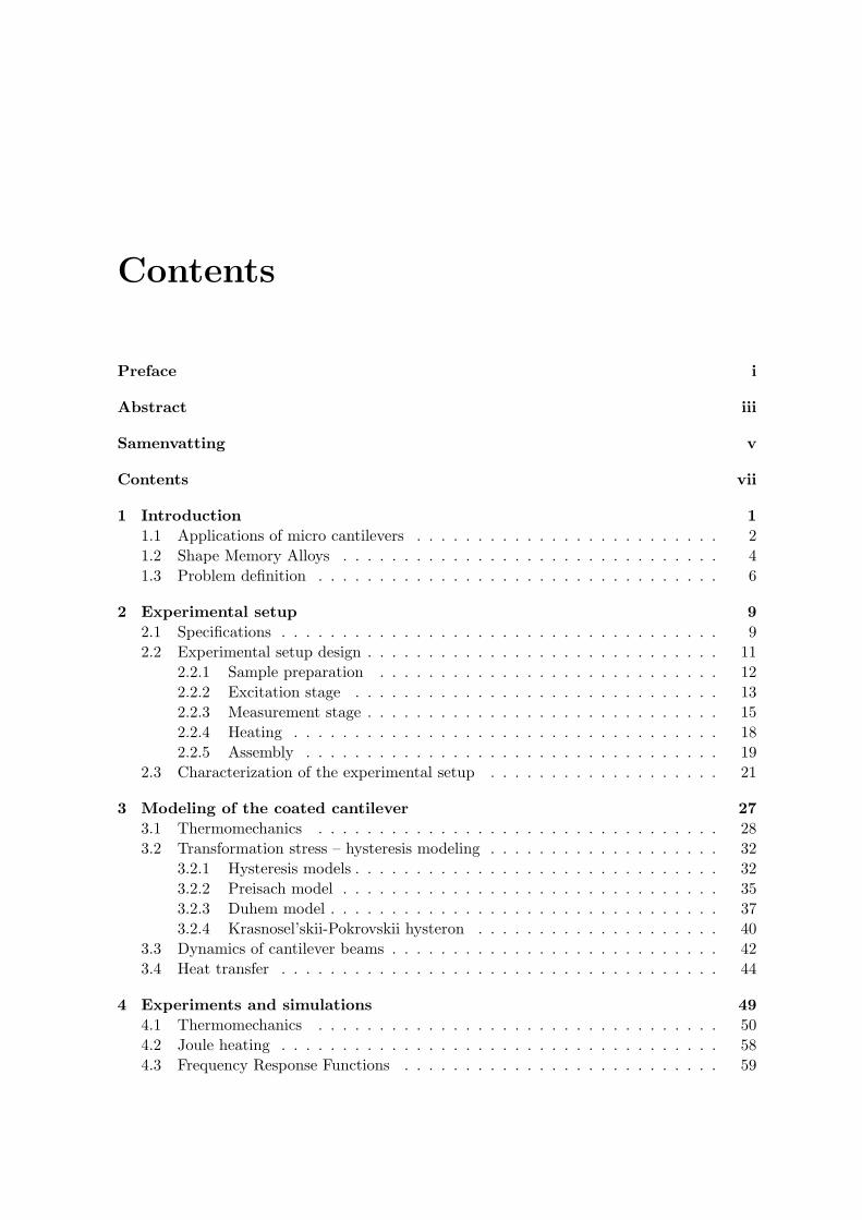
Micro cantilevers are also used as actuators. If the cantilever consists of two materials withdifferent thermal expansion coefficient, a change of temperature results in stress variationsand subsequently a deflection of the cantilever tip, called the bimorph effect. Such a designis shown in Figure 1.3(a). The cantilever is heated resistively by passing a current throughthe circuitry, fabricated on the cantilever and substrate. As in macro scale, these bimorphstructures can be used as switches or levers. Another actuator design is shown in Figure1.3(b). This is an electrostatic switch. A potential difference over the source and the gateresults in an electrostatic force, attracting the cantilever tip to the drain. Another actuationprinciple is to use magnetic force to deflect the beam or to laminate the cantilever withpiezoelectric material.
(a) A thermally activated micro cantileveractuator. An electrical circuit is deposited onthe cantilever and substrate. Passing a currentthrough the circuit heats up the cantilever [Sou07].
GateSource
Drain
25 kV
10 u39 mm
cantilever
(b) An electrostatic switch. The source and gateare responsible for actuation of the cantilever. Thecantilever makes contact with the drain if thethreshold potential difference is exceeded [Mic08].
Figure 1.3: SEM pictures of the application of micro cantilevers as actuators.
4 Introduction
1.2 Shape Memory Alloys
Shape Memory Alloys are materials, showing reversible martensitic phase transformations,induced by temperature or stress [OR05,Wan07]. These phase transformations can result inthe so-called Shape Memory Effect and the Superelasticity Effect.
The Shape Memory Effect is a process, where a seemingly plastic deformation in Martensitephase is undone by heating the material to Austenite phase, called self-accommodation of thecrystals. The recovery of the original shape in Austenite can be seen as a ’memorized’ shape.The Superelasticity effect is the process of recovery of large strains (up to 10%) at certaintemperatures, during a load cycle. The reason for this recovery is the stress-induced phasetransformation. In Figure 1.4 both processes are shown in the temperature-stress plane.It can be seen in the figure, that the phase transition temperatures depend on the stresslevels and that transformation can occur both temperature-induced and stress-induced. Thisdependence is described by Clausius-Clapeyron equation
dσ
dT= c, (1.1)
where c is a constant. The temperature dependence of the transformation temperatures isvisualized as the solid lines.
Austenite
Martensite
R
Str
ess-induced
phase tra
nsfo
rmation
Temperature-induced
phase transformation
Phase transition
Mechanic
al
loadin
g
Temperature T
Str
ess
σ
As0Af0
Ms0Mf0
Figure 1.4: Critical temperature and stress for phase transformation in an SMA. TheClausius-Clapeyron relation is drawn as the solid lines. The dashed line indicatethe R-phase transition temperatures. Temperature-induced and stress-inducedtransformation is indicated with the arrows. The temperatures below indicate the zerostress transformation temperatures, further explained below. A graphical representationof the crystal structure in various phases is also shown.
1.2 Shape Memory Alloys 5
For temperature induced transformation the stress level remains constant, while thetransformation takes place. When cooling from high temperature at constant stress nomacroscopic change takes place, but the crystals reorient from the Austenite crystal structureto Martensite, which can have several crystal structures. If no mechanical load is applied,heating again does not change the macroscopic shape of the material. When the materialis deformed in Martensite shape, a seemingly plastic deformation on macroscopic scale isobtained. This appears like plastic deformation, because the strain-stress curve is similar.However, when the heating the material again, the Austenite phase is formed and the originalshape of the material is recovered.
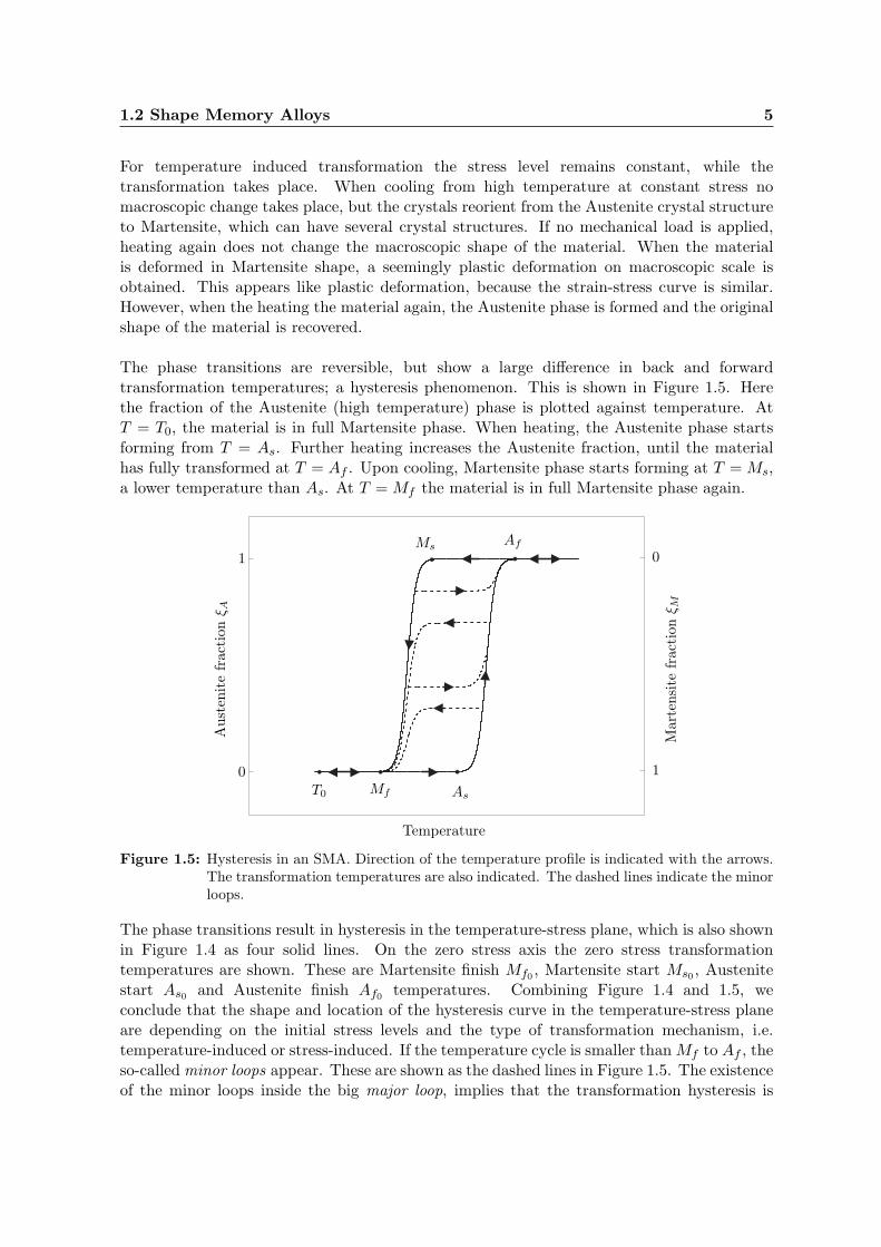
The phase transitions are reversible, but show a large difference in back and forwardtransformation temperatures; a hysteresis phenomenon. This is shown in Figure 1.5. Herethe fraction of the Austenite (high temperature) phase is plotted against temperature. AtT = T0, the material is in full Martensite phase. When heating, the Austenite phase startsforming from T = As. Further heating increases the Austenite fraction, until the materialhas fully transformed at T = Af . Upon cooling, Martensite phase starts forming at T = Ms,a lower temperature than As. At T = Mf the material is in full Martensite phase again.
0
0 1
1Ms
Mf As
Af
T0
Temperature
Aust
enit
efr
acti
onξ A
Mar
tensi
tefr
acti
onξ M
Figure 1.5: Hysteresis in an SMA. Direction of the temperature profile is indicated with the arrows.The transformation temperatures are also indicated. The dashed lines indicate the minorloops.
The phase transitions result in hysteresis in the temperature-stress plane, which is also shownin Figure 1.4 as four solid lines. On the zero stress axis the zero stress transformationtemperatures are shown. These are Martensite finish Mf0
, Martensite start Ms0, Austenite
start As0and Austenite finish Af0
temperatures. Combining Figure 1.4 and 1.5, weconclude that the shape and location of the hysteresis curve in the temperature-stress planeare depending on the initial stress levels and the type of transformation mechanism, i.e.temperature-induced or stress-induced. If the temperature cycle is smaller than Mf to Af , theso-called minor loops appear. These are shown as the dashed lines in Figure 1.5. The existenceof the minor loops inside the big major loop, implies that the transformation hysteresis is
6 Introduction
strongly dependent on the history of the temperature cycles.
Nickel-Titanium
One of the most commonly used SMA materials is Nickel-Titanium (NiTi). The transitiontemperatures of NiTi greatly depend on the composition and on heat treatments. It isreported that for equiatomic NiTi (∼ 50 wt% Ni), when stress levels are low, an intermediatephase transition takes place, the R-phase transition [OR05]. The appearance of this R-phaseonly at low stress levels is also explained by the Clausius-Clapeyron equation from Figure1.4. The R-phase transition temperature evolves along the dashed line. We can see that athigh temperatures the transition temperature equals the Austenite transition temperature,so the material transforms instantly from Martensite to Austenite.
The phase transformation in equiatomic NiTi is accompanied with large changes in thematerial properties of the alloy. A change in Young’s modulus and thermal expansion ofup to 100% is observed. These properties influence the mechanics and dynamics of thematerial significantly. Furthermore, the sliding of crystal planes, especially during R-phasetransformation gives friction, which results in high damping [Wut03]. The change of theseproperties during phase transition will have influence on the mechanical and dynamicalbehavior of materials, containing NiTi.
1.3 Problem definition
Micro cantilevers, used as sensors and actuators, can benefit in several ways from an SMAcoating. The basis for this benefit is that the properties of the film can be changed, havinginfluence on the behavior of the cantilever. This may increase the performance of thecantilever in a situation where the operation requirements change.
For the AFM cantilever and the bio-mechanical sensor (Figure 1.2), small disturbances havelarge influence on the measurement, because the cantilevers are sensitive. Since the SMA filmin some cases shows large damping during phase transformation, phase transformations canbe seen as a means of active damping. The temperature of the film then determines whetherthe damping is ’switched on’ or not. Another benefit is that the cantilever has a tunablestiffness. This means that for specific cases one could choose to do the measurement witha stiffer cantilever. It is to be investigated if the influence of the phase transformations onthe stiffness and damping is significant for this application. The bimorph cantilever (Figure1.3(a)) is a system that uses the deposited material to deform, as a result of a thermalmismatch. As discussed above, an SMA film can show large strain recovery for temperature-and stress-induced transformation, which can greatly increase the stroke of the actuator.The electrostatic switch (Figure 1.3(b)) can benefit from an SMA film, because the switchhas a tunable switching threshold. If the stiffness can be tuned, the applied voltage forattracting the cantilever to the drain varies. This makes the switch more versatile, thoughstill relatively simple to manufacture.
In a larger scope, an SMA thin film can be deposited on other micro or macro structures.If we are able to change the temperature of the film, damping or stiffness can be added ifdesired. Depositing the film on a micro cantilever gives the opportunities of investigating the
1.3 Problem definition 7
suitability of using SMA on micro scale. It also gives more insights in the thermomechanicalbehavior of the material, which still is a relevant research topic.
The problem definition is formulated as follows:
”Investigate the suitability of using a Shape Memory Alloy coating on micro cantilevers toactively influence its dynamic behavior.”
The first step is to analyze the requirements for measuring and analyzing the behaviorof the coated cantilever. An experimental setup is designed, meeting these requirements.Samples of NiTi coated micro cantilevers are prepared for thermomechanical and dynamicalmeasurements. Secondly, the thermomechanical behavior of the cantilever is analyzed. Withthese results a prediction can be made about the dynamical behavior. Characterization of thethermomechanical and dynamical behavior of the cantilever is done using the experimentalsetup and is compared to analytical results. A semi-empirical model, based on theoreticalanalysis and experimental results is formulated, which is useful for further assessment of thepossibilities and limitations of the proposed design.
Outline of the report
The report is built up as follows. Chapter 2 deals with the design and realization of anexperimental setup for dynamic and thermal analysis of NiTi coated micro cantilevers. InChapter 3, modeling approaches for the electrothermal, thermomechanical and dynamicalbehavior are presented, useful for understanding the behavior of the system. Measurementresults are discussed in Chapter 4. We also propose a semi-empirical model to describe thebehavior of the coated cantilever. Finally, conclusions and recommendations are stated inChapter 5.

Chapter 2
Experimental setup
For thermomechanical experiments, measurement equipment is available at the Multi-ScaleLaboratory at the department of Mechanical Engineering at the TU/e. To investigate thedynamical response of the micro cantilevers, a specialized experimental setup is designed. AnAFM would also do, but availability issues, software limitations and lack of specificationslimit its usefulness for this project. Furthermore, the objective is to investigate the dynamicproperties of NiTi coated micro cantilevers for varying temperature. An experimental setupis designed, capable of exciting the cantilevers, varying their temperature and measuring thevibrations. This gives insight in the possibilities, limitations and applicability of the designand provides a realistic view on this approach on dynamic control at micro scale, using aNiTi coating. The specifications of the setup, the functions of its components, calibrationand preliminary measurements are discussed in the following sections.
2.1 Specifications
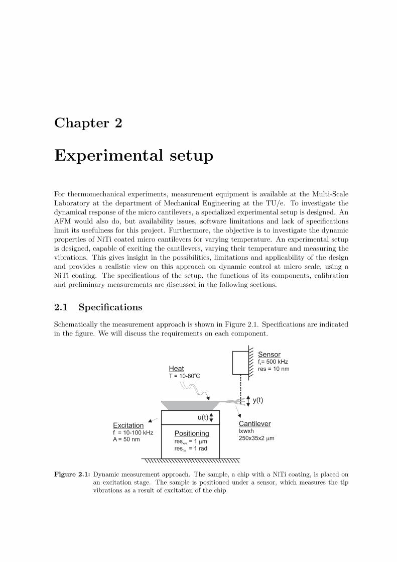
Schematically the measurement approach is shown in Figure 2.1. Specifications are indicatedin the figure. We will discuss the requirements on each component.
w
Figure 2.1: Dynamic measurement approach. The sample, a chip with a NiTi coating, is placed onan excitation stage. The sample is positioned under a sensor, which measures the tipvibrations as a result of excitation of the chip.
10 Experimental setup
Cantilevers
Uncoated micro cantilevers with known properties are coated with an equiatomic NiTi thinfilm by means of sputter deposition. As deposited, the material is amorphous. The film isannealed in order to crystallize it, giving the material its phase transformation properties. Thecantilever chips have to be properly handled and suspended for assembly into the excitationstage and for heating the film.
Excitation and measurement
Depending on its application, the resonance frequency of an AFM cantilever can rangefrom 5 up to 500 kHz. In contact mode, the probes are required to be sensitive to smallforce fluctuations, so low stiffness is desired, giving a low resonance frequency (recallthat ω0 =
√
k/m). For tapping mode AFM, stiff cantilevers (thus having a high resonancefrequency) are used. The cantilever is operated near or at its resonance frequency. Interactionwith the substrate results in shifts of the resonance frequency, the amplitude and the phase,which gives information about the sample. Introducing damping or additional shifts inthe resonance frequency is not desired. A NiTi coated cantilever will not improve themeasurement in tapping mode, we therefore concentrate on low stiffness cantilevers.
In contact mode Atomic Force Microscopy, the cantilever moves across the surface of thesample at low speed, typically at 0.1 Hz - 1 Hz over a stroke of several microns. A shock orother disturbance can excite the cantilever, causing it to vibrate, which in this case is notdesirable. It is therefore useful to investigate the possibility of changing the dynamics in sucha case. These cantilevers generally have a resonance frequency between 10 kHz and 100 kHz.Excitation to and beyond the resonance frequency is necessary. To measure the response tothis excitation, a measurement system capable of high frequency dynamic measurements anddata acquisition hardware and software with high sampling rates is required.
In typical AFM measurements, the amplitude of excitation of a cantilever in tapping mode isin the order of tenths of nanometers. Larger amplitudes can cause breaking, delamination orunstable behavior. Small amplitudes (±50 nm) at high frequencies (10-100 kHz) are requiredfor analyzing the cantilevers. Measuring these vibrations requires a high sample rate and aresolution in the order of nanometers.
Heating
Changing the temperature of the NiTi film is expected to change its mechanical and dynamicalproperties significantly, as a result of phase transformations. For an equiatomic NiTi film ona glass or Silicon substrate, the transition temperatures are reported in the range of −10C to100C [Wan07]. Relevant temperatures for dynamic operation may differ. A way of heatingand cooling the NiTi film without perturbing the excitation or obstructing the sensor isrequired. Moreover, the temperature needs to be dynamically changed, so fast heating andcooling is preferred.
2.2 Experimental setup design 11
2.2 Experimental setup design
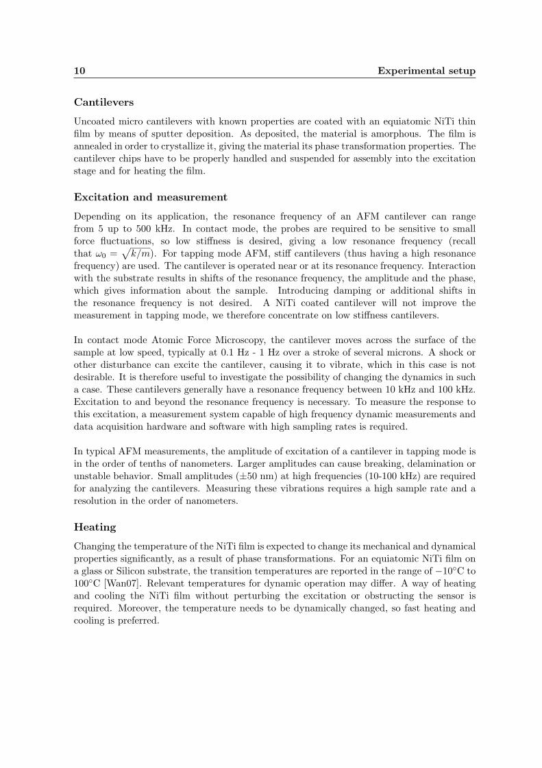
The proposed setup is shown in Figure 2.2.
LDGU
LDGU AMP
Kinematic mount
Piezo element
X,Y,Z,manual
translation & rotationstage
f,q Piezo amplifier&
High voltagepower supply
Current sourceDAQ I/O
Figure 2.2: Schematic representation of the final experimental setup.
Here we distinguish
- a NiTi coated cantilever chip, supported by a steel mounting plate for easy handlingand positioning;
- a piezo element with amplifier and high voltage power supply, to excite the cantileverchip to high frequencies;
- an optical measurement head with amplifier, supported by a stiff measurement frame;
- a five degree of freedom manual positioning stage, to position the cantilevers in the focalpoint of the optical measurement head;
- a current source and wire contacts to the NiTi film, to resistively heat the film (Jouleheating);
- data acquisition hardware and software.
These components and their assembly are discussed in the following sections.
12 Experimental setup
2.2.1 Sample preparation
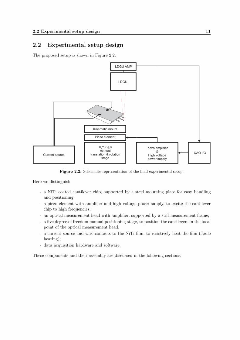
The micro cantilevers, used in these experiments, are supplied by µMasch [Mik07]. Thecantilevers are tipless, rectangular and made of single crystal Silicon. A chip containssix cantilevers of different length and thus have a different resonance frequency. Typicaldimensions are lxwxh = 300x35x2 µm. The chips have the dimensions lxwxh = 3.4x1.6x0.4mm. Other specifications are found in Appendix C.
The cantilever chips are coated at Harvard University by Dr. Xi Wang of Prof. Vlassak’sGroup. A thin film of equiatomic NiTi approximately 1µm thick is co-sputtered under highvacuum (1·10−4 mTorr) at room temperature. After sputtering, the film is annealed in thesame vacuum at 500C for approximately 30 minutes, to fully crystalize the film. A SEMpicture of the coated cantilever chip is shown in Figure 2.3.
Figure 2.3: SEM image of NiTi coated Silicon cantilevers on chip NSC12. The glue, used for attachingthe chip on the supporting plate, is seen, as well as a wire, glued to the NiTi film. Thethree cantilevers of different length are distinguished on the right hand side of the chip.
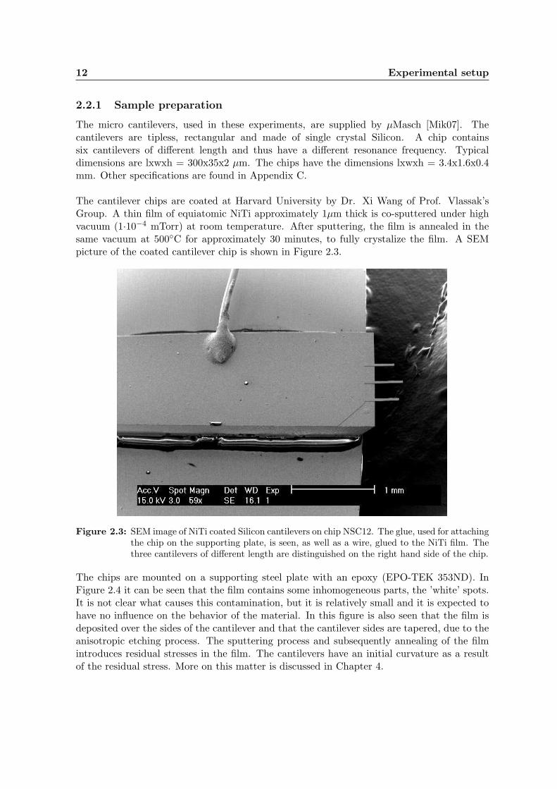
The chips are mounted on a supporting steel plate with an epoxy (EPO-TEK 353ND). InFigure 2.4 it can be seen that the film contains some inhomogeneous parts, the ’white’ spots.It is not clear what causes this contamination, but it is relatively small and it is expected tohave no influence on the behavior of the material. In this figure is also seen that the film isdeposited over the sides of the cantilever and that the cantilever sides are tapered, due to theanisotropic etching process. The sputtering process and subsequently annealing of the filmintroduces residual stresses in the film. The cantilevers have an initial curvature as a resultof the residual stress. More on this matter is discussed in Chapter 4.
2.2 Experimental setup design 13
(a) Tip of the coated cantilever. The sides of thecantilever are tapered, due to the anisotropic etchingprocess. The white spots are also shown.
(b) Cantilever connection to chip. The NiTi film iscovering the chip well.
Figure 2.4: SEM pictures of the deposited film on the Silicon cantilever.
2.2.2 Excitation stage
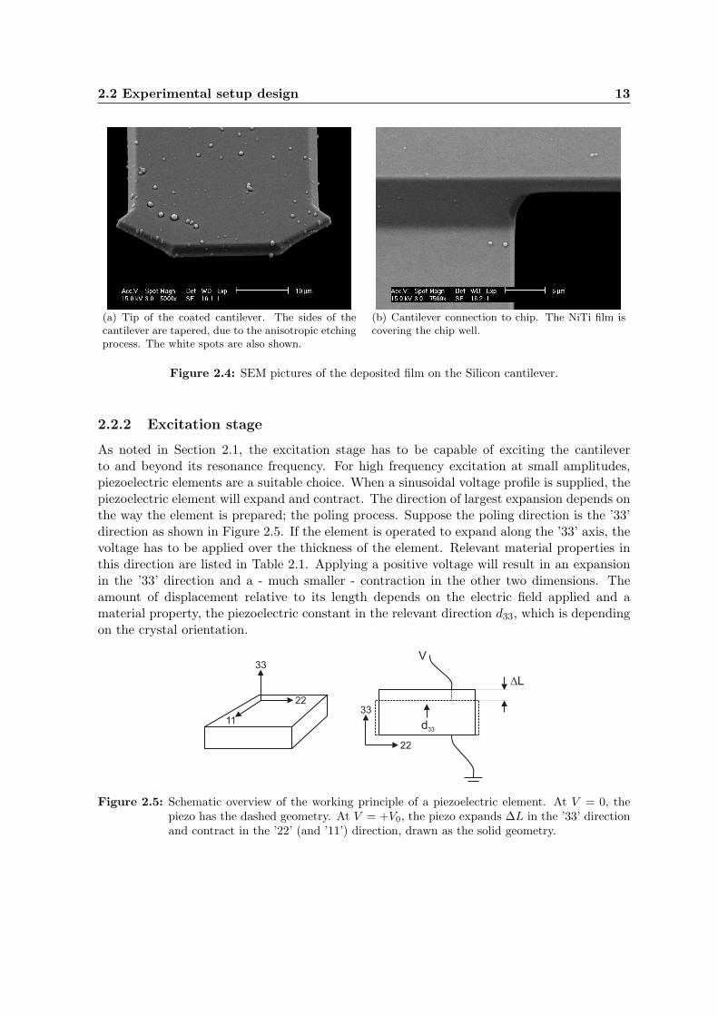
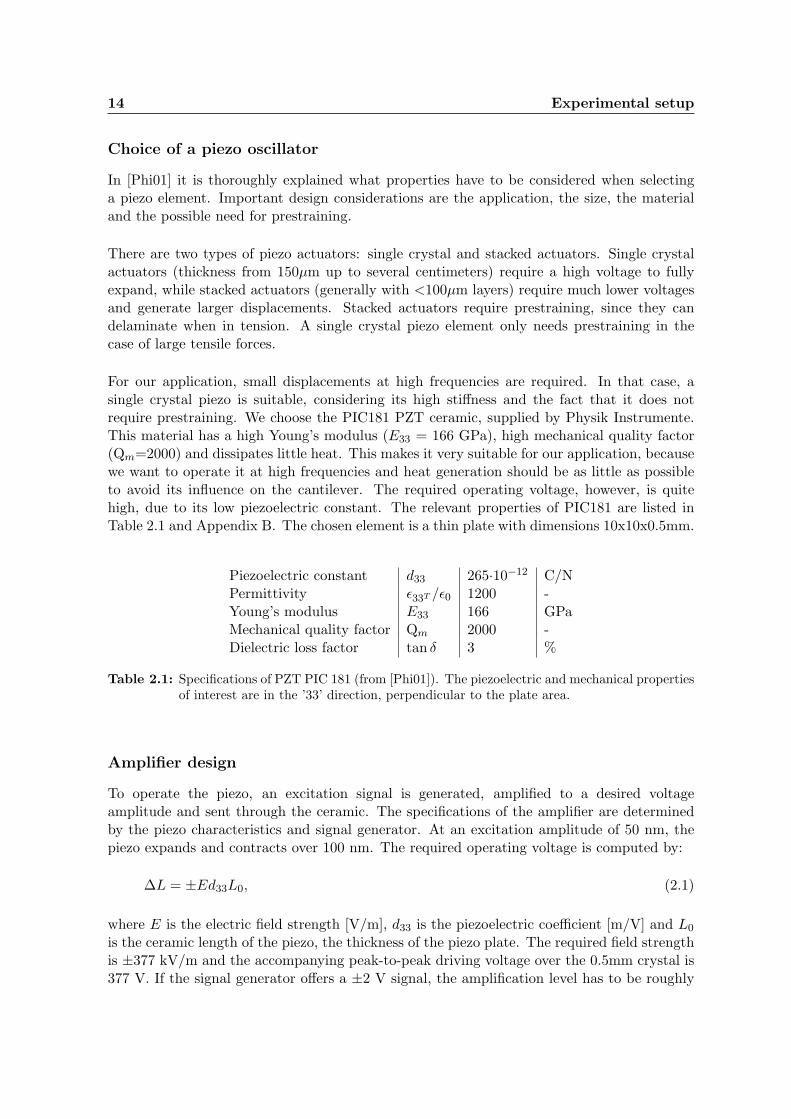
As noted in Section 2.1, the excitation stage has to be capable of exciting the cantileverto and beyond its resonance frequency. For high frequency excitation at small amplitudes,piezoelectric elements are a suitable choice. When a sinusoidal voltage profile is supplied, thepiezoelectric element will expand and contract. The direction of largest expansion depends onthe way the element is prepared; the poling process. Suppose the poling direction is the ’33’direction as shown in Figure 2.5. If the element is operated to expand along the ’33’ axis, thevoltage has to be applied over the thickness of the element. Relevant material properties inthis direction are listed in Table 2.1. Applying a positive voltage will result in an expansionin the ’33’ direction and a - much smaller - contraction in the other two dimensions. Theamount of displacement relative to its length depends on the electric field applied and amaterial property, the piezoelectric constant in the relevant direction d33, which is dependingon the crystal orientation.
33
22
11
DL
d33
V
33
22
Figure 2.5: Schematic overview of the working principle of a piezoelectric element. At V = 0, thepiezo has the dashed geometry. At V = +V0, the piezo expands ∆L in the ’33’ directionand contract in the ’22’ (and ’11’) direction, drawn as the solid geometry.
14 Experimental setup
Choice of a piezo oscillator
In [Phi01] it is thoroughly explained what properties have to be considered when selectinga piezo element. Important design considerations are the application, the size, the materialand the possible need for prestraining.
There are two types of piezo actuators: single crystal and stacked actuators. Single crystalactuators (thickness from 150µm up to several centimeters) require a high voltage to fullyexpand, while stacked actuators (generally with <100µm layers) require much lower voltagesand generate larger displacements. Stacked actuators require prestraining, since they candelaminate when in tension. A single crystal piezo element only needs prestraining in thecase of large tensile forces.
For our application, small displacements at high frequencies are required. In that case, asingle crystal piezo is suitable, considering its high stiffness and the fact that it does notrequire prestraining. We choose the PIC181 PZT ceramic, supplied by Physik Instrumente.This material has a high Young’s modulus (E33 = 166 GPa), high mechanical quality factor(Qm=2000) and dissipates little heat. This makes it very suitable for our application, becausewe want to operate it at high frequencies and heat generation should be as little as possibleto avoid its influence on the cantilever. The required operating voltage, however, is quitehigh, due to its low piezoelectric constant. The relevant properties of PIC181 are listed inTable 2.1 and Appendix B. The chosen element is a thin plate with dimensions 10x10x0.5mm.
Piezoelectric constant d33 265·10−12 C/NPermittivity ǫ33T /ǫ0 1200 -Young’s modulus E33 166 GPaMechanical quality factor Qm 2000 -Dielectric loss factor tan δ 3 %
Table 2.1: Specifications of PZT PIC 181 (from [Phi01]). The piezoelectric and mechanical propertiesof interest are in the ’33’ direction, perpendicular to the plate area.
Amplifier design
To operate the piezo, an excitation signal is generated, amplified to a desired voltageamplitude and sent through the ceramic. The specifications of the amplifier are determinedby the piezo characteristics and signal generator. At an excitation amplitude of 50 nm, thepiezo expands and contracts over 100 nm. The required operating voltage is computed by:
∆L = ±Ed33L0, (2.1)
where E is the electric field strength [V/m], d33 is the piezoelectric coefficient [m/V] and L0
is the ceramic length of the piezo, the thickness of the piezo plate. The required field strengthis ±377 kV/m and the accompanying peak-to-peak driving voltage over the 0.5mm crystal is377 V. If the signal generator offers a ±2 V signal, the amplification level has to be roughly
2.2 Experimental setup design 15
100. To compute the current consumption, the capacitance C [F] is an important parameter:
C ≈ nǫ33T
A
ds, (2.2)
where n is the number of layers, ǫ33T is the permittivity [As/Vm], A is the electrode surfacearea and ds is the layer thickness. The permittivity is often expressed as a multiple of theelectric constant ǫ0 = 8.854 · 10−12 C2/N m2. For the single crystal piezo plate with size10x10x0.5mm, the capacitance is C = 2.12 nF. The maximum operating current is
imax ≈ fπCUp−p = 250mA, (2.3)
for sinusoidal operation, with frequency f and peak-to-peak drive voltage Up−p.
From (2.2) it is clear that stacked piezo’s have a much higher capacitance; n increases and ds
decreases. This introduces some problems concerning the operation of the actuator, becausean amplifier has to supply a high frequency signal to the piezo, at the appropriate voltageamplitude. The operating voltage, though, is higher for a single crystal piezo element. Tocompare, for 10 stacked piezo elements (100 µm thick), also capable of a displacement of50nm, only ±19V is required. The capacitance is 106nF, giving a current consumption of1.2A at 100kHz. High frequency amplifiers cannot handle these high capacitance loads, whilea high operating voltage is less problematic.
The amplifier circuitry was designed by Michael Hopper and built by the Central TechnicalService of the TU/e. The electrical circuit layout is found in Appendix D. The amplifieroperates between 0-400V and can handle a current consumption up to 600 mA. Preliminarytesting shows that a drive frequency of up to 100 kHz with an amplitude of 200V can bereached, using an input signal with an amplitude of 2V, so the amplifier is designed wellwithin specifications. More on the operation of the piezo will be discussed in Section 2.3.
Heat dissipation
During operation, the piezo generates heat, proportional to its dielectric loss factor, tan δ:
P ≈ π
4tan δfCU2
p−p. (2.4)
The loss factor for PIC181 PZT is 3%, giving a thermal power of P ≈ 0.7W. To dissipatethat heat, the piezo is placed on top of an aluminum heatsink, so overheating is avoided.
2.2.3 Measurement stage
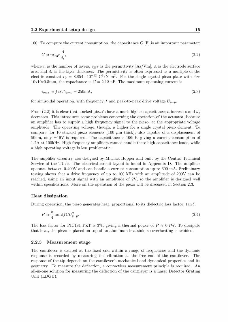
The cantilever is excited at the fixed end within a range of frequencies and the dynamicresponse is recorded by measuring the vibration at the free end of the cantilever. Theresponse of the tip depends on the cantilever’s mechanical and dynamical properties and itsgeometry. To measure the deflection, a contactless measurement principle is required. Anall-in-one solution for measuring the deflection of the cantilever is a Laser Detector GratingUnit (LDGU).
16 Experimental setup
An LDGU consists of a laser source, photodiodes and a grating. Additionally, mirrorsand lenses are placed to guide and focus the laser light [Pri02]. In Figure 2.6 a schematicrepresentation of the general working principle is shown. The laser beam is split by a beamsplitter, guided through the grating and focused on the surface. When exactly in focus, thereflected light follows the exact same path back through the lens, but at the grating it isrefracted and directed to the diodes. The diodes are placed such that when the light beamsare in focus, the reflected beams are also focused on the diodes, resulting in a small lightspot and a low output current of the diodes. When the object moves towards or away fromthe focal point of the laser beam, the light spots grow and move - due to different diffractionthrough the grating - and the output currents differ. The analog signal of the diode couplesis subtracted, which is a measure of the displacement of the object.
Figure 2.6: Measurement principle of a Laser Detector Grating Unit (LDGU) [Pri02].
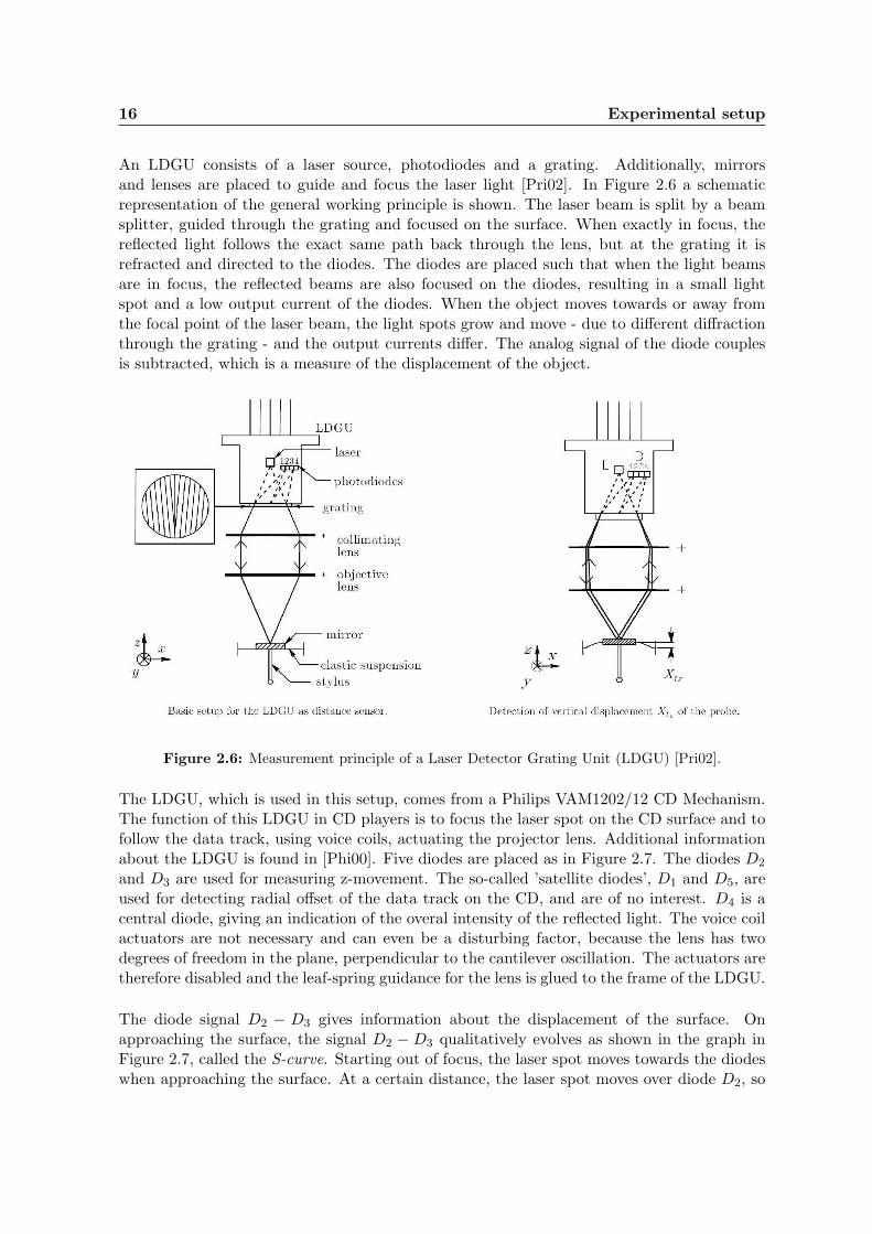
The LDGU, which is used in this setup, comes from a Philips VAM1202/12 CD Mechanism.The function of this LDGU in CD players is to focus the laser spot on the CD surface and tofollow the data track, using voice coils, actuating the projector lens. Additional informationabout the LDGU is found in [Phi00]. Five diodes are placed as in Figure 2.7. The diodes D2
and D3 are used for measuring z-movement. The so-called ’satellite diodes’, D1 and D5, areused for detecting radial offset of the data track on the CD, and are of no interest. D4 is acentral diode, giving an indication of the overal intensity of the reflected light. The voice coilactuators are not necessary and can even be a disturbing factor, because the lens has twodegrees of freedom in the plane, perpendicular to the cantilever oscillation. The actuators aretherefore disabled and the leaf-spring guidance for the lens is glued to the frame of the LDGU.
The diode signal D2 − D3 gives information about the displacement of the surface. Onapproaching the surface, the signal D2 − D3 qualitatively evolves as shown in the graph inFigure 2.7, called the S-curve. Starting out of focus, the laser spot moves towards the diodeswhen approaching the surface. At a certain distance, the laser spot moves over diode D2, so
2.2 Experimental setup design 17
D2
D3
Satellite spot
Centralaperture
Satellite spot
Peak-peak value
Am
plit
ud
eD
2-D
3
z (towards disk)
D1
D4
D5
D2
D3
Figure 2.7: Diode layout and s-curve of the Sharp GH6C005B3A LDGU (from [Phi00]).
D2−D3 is positive. Further approaching the surface, both D2 and D3 are illuminated equally,so D2 − D3 = 0. Moving along, D3 receives more light, so the signal becomes negative. Ifthe surface is too close, the laser spot is not illuminating the diode anymore, and the signalvanishes again. The output currents can be related to the displacement of the surface. ThisLDGU can detect amplitudes up to 12 µm.
Data acquisition
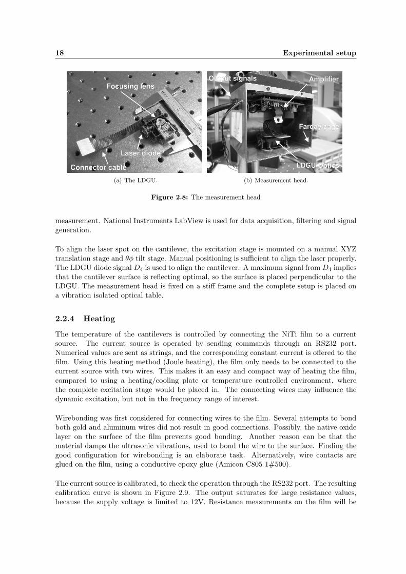
A flat cable connects the LDGU to a power source and the diode signals can also be acquired.The output currents (in the order of µA) are amplified and converted to a voltage by aninstrumentation amplifier. The amplifier circuit can be found in Appendix E. To shield themeasurement stage and amplifier from surrounding electromagnetic noise, a brass Faradaycage is built. This cage also protects the equipment and makes positioning and handlingof the measurement stage easier. BNC connectors and coax cables shield the diode signals,directed to the data acquisition hardware. A picture of the LDGU and the final measurementhead is shown in Figure 2.8.
To acquire the diode signals and to excite the piezo at high frequency, high speed DataAquisition (DAQ) hardware is required. The resonance frequency of the cantilevers isexpected in a range up to 100 kHz. The Nyquist Shannon sampling theorem states thatfor a frequency to be reconstructible, the sampling rate of the signal must be at least twotimes higher than this frequency. A rule of thumb is to use five times the frequency, to avoidaliasing and to be working well within the limits of the hardware.
The NI-USB 6251 from National Instruments is chosen, for its easy connection and highsample rate (1.25 MHz). When two signals are acquired simultaneously, the sample rate isroughly half the maximum rate. BNC connectors are made in the casing of the NI-USB6251, because the standard supplied flatcable introduced unacceptable noise levels in the
18 Experimental setup
Connector cable
Laser diode
Focusing lens
(a) The LDGU.
Amplifier
LDGU Optics
Output signals
Farday cage
(b) Measurement head.
Figure 2.8: The measurement head
measurement. National Instruments LabView is used for data acquisition, filtering and signalgeneration.
To align the laser spot on the cantilever, the excitation stage is mounted on a manual XYZtranslation stage and θφ tilt stage. Manual positioning is sufficient to align the laser properly.The LDGU diode signal D4 is used to align the cantilever. A maximum signal from D4 impliesthat the cantilever surface is reflecting optimal, so the surface is placed perpendicular to theLDGU. The measurement head is fixed on a stiff frame and the complete setup is placed ona vibration isolated optical table.
2.2.4 Heating
The temperature of the cantilevers is controlled by connecting the NiTi film to a currentsource. The current source is operated by sending commands through an RS232 port.Numerical values are sent as strings, and the corresponding constant current is offered to thefilm. Using this heating method (Joule heating), the film only needs to be connected to thecurrent source with two wires. This makes it an easy and compact way of heating the film,compared to using a heating/cooling plate or temperature controlled environment, wherethe complete excitation stage would be placed in. The connecting wires may influence thedynamic excitation, but not in the frequency range of interest.
Wirebonding was first considered for connecting wires to the film. Several attempts to bondboth gold and aluminum wires did not result in good connections. Possibly, the native oxidelayer on the surface of the film prevents good bonding. Another reason can be that thematerial damps the ultrasonic vibrations, used to bond the wire to the surface. Finding thegood configuration for wirebonding is an elaborate task. Alternatively, wire contacts areglued on the film, using a conductive epoxy glue (Amicon C805-1#500).
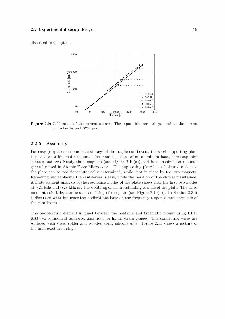
The current source is calibrated, to check the operation through the RS232 port. The resultingcalibration curve is shown in Figure 2.9. The output saturates for large resistance values,because the supply voltage is limited to 12V. Resistance measurements on the film will be
2.2 Experimental setup design 19
discussed in Chapter 4.
−500 0 500 1000 1500 2000 2500
0
500
1000
1500
no loadR=5 ΩR=10 ΩR=15 ΩR=20 Ω
Ticks [-]
Curr
ent
[mA
]
Figure 2.9: Calibration of the current source. The input ticks are strings, send to the currentcontroller by an RS232 port.
2.2.5 Assembly
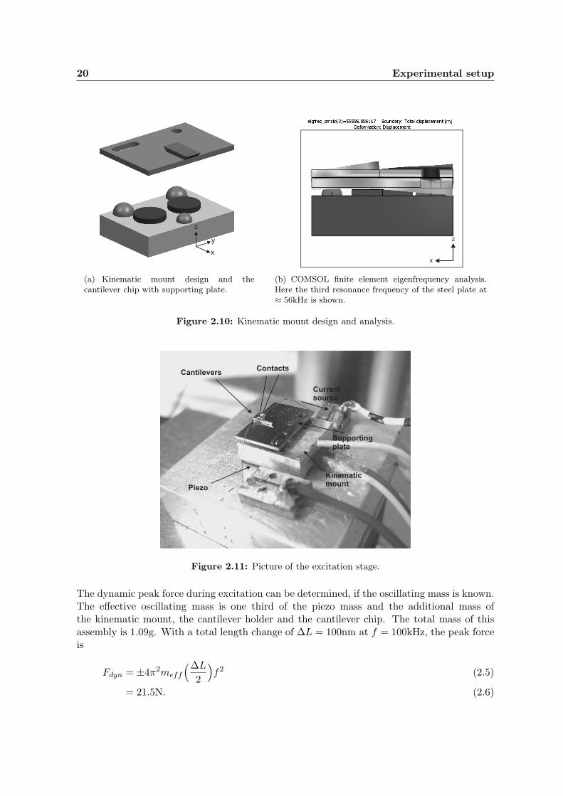
For easy (re)placement and safe storage of the fragile cantilevers, the steel supporting plateis placed on a kinematic mount. The mount consists of an aluminum base, three sapphirespheres and two Neodymium magnets (see Figure 2.10(a)) and it is inspired on mounts,generally used in Atomic Force Microscopes. The supporting plate has a hole and a slot, sothe plate can be positioned statically determined, while kept in place by the two magnets.Removing and replacing the cantilevers is easy, while the position of the chip is maintained.A finite element analysis of the resonance modes of the plate shows that the first two modesat ≈21 kHz and ≈28 kHz are the wobbling of the freestanding corners of the plate. The thirdmode at ≈56 kHz, can be seen as tilting of the plate (see Figure 2.10(b)). In Section 2.3 itis discussed what influence these vibrations have on the frequency response measurements ofthe cantilevers.
The piezoelectric element is glued between the heatsink and kinematic mount using HBMX60 two component adhesive, also used for fixing strain gauges. The connecting wires aresoldered with silver solder and isolated using silicone glue. Figure 2.11 shows a picture ofthe final excitation stage.
20 Experimental setup
z
y
x
(a) Kinematic mount design and thecantilever chip with supporting plate.
x
z
(b) COMSOL finite element eigenfrequency analysis.Here the third resonance frequency of the steel plate at≈ 56kHz is shown.
Figure 2.10: Kinematic mount design and analysis.
CantileversContacts
Supportingplate
Kinematicmount
Piezo
Currentsource
Figure 2.11: Picture of the excitation stage.
The dynamic peak force during excitation can be determined, if the oscillating mass is known.The effective oscillating mass is one third of the piezo mass and the additional mass ofthe kinematic mount, the cantilever holder and the cantilever chip. The total mass of thisassembly is 1.09g. With a total length change of ∆L = 100nm at f = 100kHz, the peak forceis
Fdyn = ±4π2meff
(∆L
2
)
f2 (2.5)
= 21.5N. (2.6)

2.3 Characterization of the experimental setup 21
The required stiffness of the construction then is
kT =Fdyn
∆L/2= 430 · 106 N/m. (2.7)
The stiffness of the piezo in the excitation direction is
k33 =CD
33A
L= 33.2 · 1010 N/m, (2.8)
which is much higher than the required stiffness, so the piezo element does not needprestraining and will hold the dynamic forces for our purposes.
2.3 Characterization of the experimental setup
To isolate the cantilever’s frequency response from the piezo excitation, the influence of theperipheral equipment is investigated.
To investigate the operation of the piezo amplifier, the Frequency Response Function (FRF)of the amplifier output signal is compared to the FRF of the amplifier input signal. The powersupply and piezo amplifier will distort the input signal, generated by the software. In Figure2.12 it can be seen that the amplifier contains a highpass filter. Excitation frequencies in therange of 10 kHz to 100 kHz are amplified best, according to the specifications. A maximumamplification level of ±80 is achieved in this frequency range.
100
101
102
101
102
Frequency [kHz]
Outp
ut/
Input
[-]
Figure 2.12: Frequency Response Function of the amplifier output to the signal generator input.
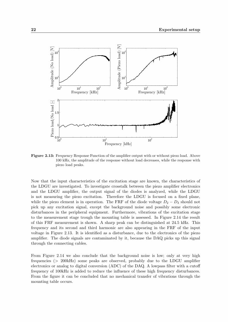
If the piezo element is connected to the amplifier, the capacitive load influences the operationof the amplifier. This is shown in Figure 2.13. The piezo load only affects the FRF of theamplifier output above 100 kHz. This implies that for our purposes, the amplifier is able tohandle the capacitive load of the piezo element.
22 Experimental setup
100
101
102
101
102
100
101
102
101
102
100
101
102
0.5
1
1.5
2
Frequency [kHz]
Frequency [kHz]Frequency [kHz]
Am
plitu
de
(No
load
)[V
]
Am
plitu
de
(Pie
zolo
ad)
[V]
Pie
zolo
ad/N
olo
ad[-]
Figure 2.13: Frequency Response Function of the amplifier output with or without piezo load. Above100 kHz, the amplitude of the response without load decreases, while the response withpiezo load peaks.
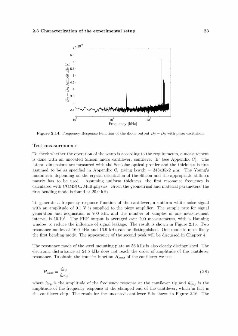
Now that the input characteristics of the excitation stage are known, the characteristics ofthe LDGU are investigated. To investigate crosstalk between the piezo amplifier electronicsand the LDGU amplifier, the output signal of the diodes is analyzed, while the LDGUis not measuring the piezo excitation. Therefore the LDGU is focused on a fixed plane,while the piezo element is in operation. The FRF of the diode voltage D2 − D3 should notpick up any excitation signal, except the background noise and possibly some electronicdisturbances in the peripheral equipment. Furthermore, vibrations of the excitation stageto the measurement stage trough the mounting table is assessed. In Figure 2.14 the resultof this FRF measurement is shown. A sharp peak can be distinguished at 24.5 kHz. Thisfrequency and its second and third harmonic are also appearing in the FRF of the inputvoltage in Figure 2.13. It is identified as a disturbance, due to the electronics of the piezoamplifier. The diode signals are contaminated by it, because the DAQ picks up this signalthrough the connecting cables.
From Figure 2.14 we also conclude that the background noise is low; only at very highfrequencies (> 200kHz) some peaks are observed, probably due to the LDGU amplifierelectronics or analog to digital conversion (ADC) of the DAQ. A lowpass filter with a cutofffrequency of 100kHz is added to reduce the influence of these high frequency disturbances.From the figure it can be concluded that no mechanical transfer of vibrations through themounting table occurs.
2.3 Characterization of the experimental setup 23
100
101
102
2.5
3
3.5
4
4.5
5
5.5
6
6.5
7x 10
−5
Frequency [kHz]
D2−
D3
Am
plitu
de
[-]
Figure 2.14: Frequency Response Function of the diode output D2 − D3 with piezo excitation.
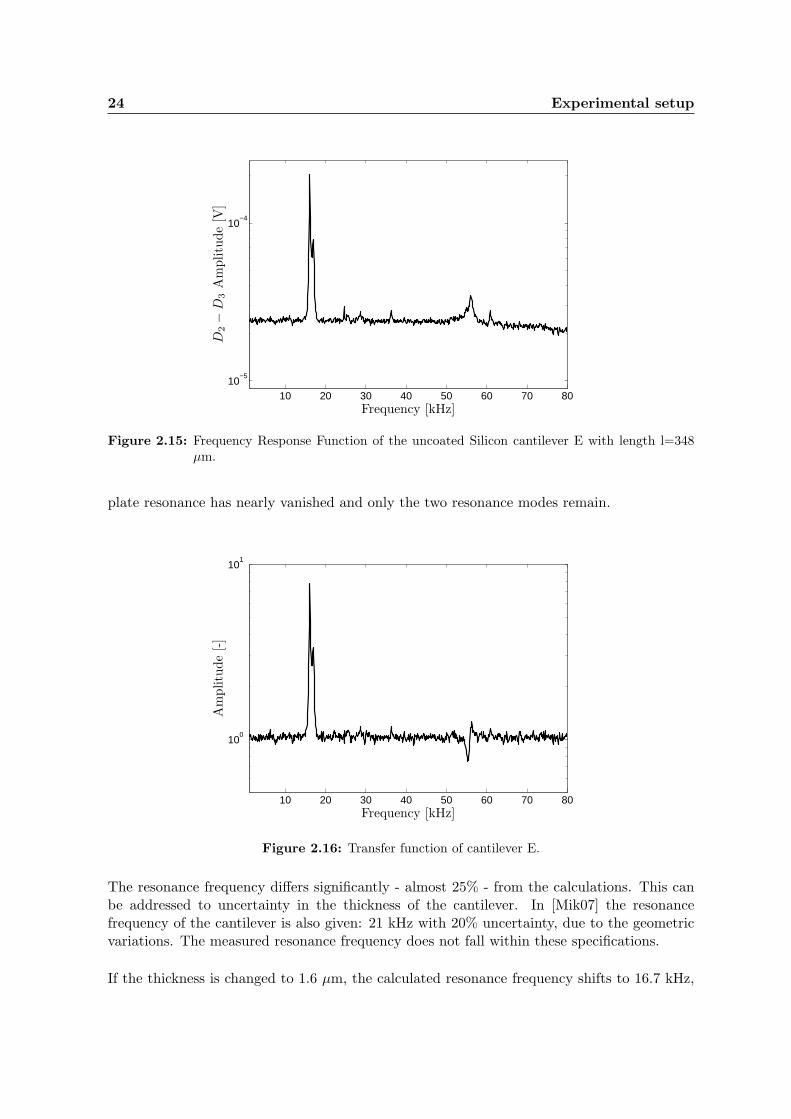
Test measurements
To check whether the operation of the setup is according to the requirements, a measurementis done with an uncoated Silicon micro cantilever, cantilever ’E’ (see Appendix C). Thelateral dimensions are measured with the Sensofar optical profiler and the thickness is firstassumed to be as specified in Appendix C, giving lxwxh = 348x35x2 µm. The Young’smodulus is depending on the crystal orientation of the Silicon and the appropriate stiffnessmatrix has to be used. Assuming uniform thickness, the first resonance frequency iscalculated with COMSOL Multiphysics. Given the geometrical and material parameters, thefirst bending mode is found at 20.9 kHz.
To generate a frequency response function of the cantilever, a uniform white noise signalwith an amplitude of 0.1 V is supplied to the piezo amplifier. The sample rate for signalgeneration and acquisition is 700 kHz and the number of samples in one measurementinterval is 10·103. The FRF output is averaged over 200 measurements, with a Hanningwindow to reduce the influence of signal leakage. The result is shown in Figure 2.15. Tworesonance modes at 16.0 kHz and 16.9 kHz can be distinguished. One mode is most likelythe first bending mode. The appearance of the second peak will be discussed in Chapter 4.
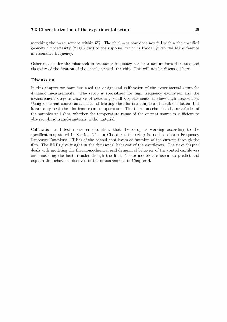
The resonance mode of the steel mounting plate at 56 kHz is also clearly distinguished. Theelectronic disturbance at 24.5 kHz does not reach the order of amplitude of the cantileverresonance. To obtain the transfer function Hcant of the cantilever we use
Hcant =ytip
ychip, (2.9)
where ytip is the amplitude of the frequency response at the cantilever tip and ychip is theamplitude of the frequency response at the clamped end of the cantilever, which in fact isthe cantilever chip. The result for the uncoated cantilever E is shown in Figure 2.16. The
24 Experimental setup
10 20 30 40 50 60 70 8010
−5
10−4
Frequency [kHz]
D2−
D3
Am
plitu
de
[V]
Figure 2.15: Frequency Response Function of the uncoated Silicon cantilever E with length l=348µm.
plate resonance has nearly vanished and only the two resonance modes remain.
10 20 30 40 50 60 70 80
100
101
Frequency [kHz]
Am
plitu
de
[-]
Figure 2.16: Transfer function of cantilever E.
The resonance frequency differs significantly - almost 25% - from the calculations. This canbe addressed to uncertainty in the thickness of the cantilever. In [Mik07] the resonancefrequency of the cantilever is also given: 21 kHz with 20% uncertainty, due to the geometricvariations. The measured resonance frequency does not fall within these specifications.
If the thickness is changed to 1.6 µm, the calculated resonance frequency shifts to 16.7 kHz,
2.3 Characterization of the experimental setup 25
matching the measurement within 5%. The thickness now does not fall within the specifiedgeometric uncertainty (2±0.3 µm) of the supplier, which is logical, given the big differencein resonance frequency.
Other reasons for the mismatch in resonance frequency can be a non-uniform thickness andelasticity of the fixation of the cantilever with the chip. This will not be discussed here.
Discussion
In this chapter we have discussed the design and calibration of the experimental setup fordynamic measurements. The setup is specialized for high frequency excitation and themeasurement stage is capable of detecting small displacements at these high frequencies.Using a current source as a means of heating the film is a simple and flexible solution, butit can only heat the film from room temperature. The thermomechanical characteristics ofthe samples will show whether the temperature range of the current source is sufficient toobserve phase transformations in the material.
Calibration and test measurements show that the setup is working according to thespecifications, stated in Section 2.1. In Chapter 4 the setup is used to obtain FrequencyResponse Functions (FRFs) of the coated cantilevers as function of the current through thefilm. The FRFs give insight in the dynamical behavior of the cantilevers. The next chapterdeals with modeling the thermomechanical and dynamical behavior of the coated cantileversand modeling the heat transfer though the film. These models are useful to predict andexplain the behavior, observed in the measurements in Chapter 4.

Chapter 3
Modeling of the coated cantilever
In Chapter 2, the experimental setup for investigating the thermal-dynamical properties ofthe cantilevers is discussed. Before conducting experiments with the NiTi coated cantileversamples, knowledge about the thermomechanical behavior is desired. This gives insightin the transformation temperatures of the material and stress variations due to the phasetransitions. Using a current source as a means of resistive heating of the NiTi film requiresknowledge about the electrothermal properties of the material, as well as heat transfer to thesurroundings.
The dynamic behavior of the cantilevers is influenced by the thermomechanical behavior. Ananalysis of the resonance frequencies and a way of investigating of the damping properties isexplained in this chapter.
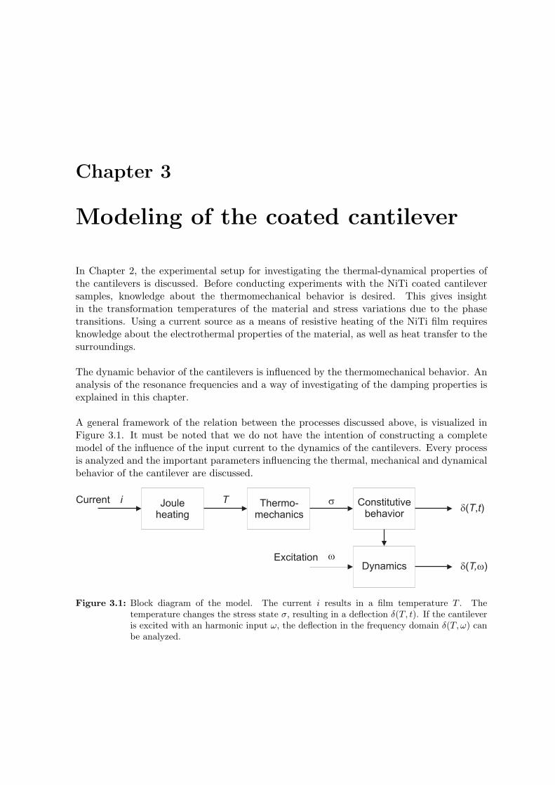
A general framework of the relation between the processes discussed above, is visualized inFigure 3.1. It must be noted that we do not have the intention of constructing a completemodel of the influence of the input current to the dynamics of the cantilevers. Every processis analyzed and the important parameters influencing the thermal, mechanical and dynamicalbehavior of the cantilever are discussed.
d w( )T,
d( , )T t
DynamicsExcitation
Current i T s
w
Figure 3.1: Block diagram of the model. The current i results in a film temperature T . Thetemperature changes the stress state σ, resulting in a deflection δ(T, t). If the cantileveris excited with an harmonic input ω, the deflection in the frequency domain δ(T, ω) canbe analyzed.
28 Modeling of the coated cantilever
3.1 Thermomechanics
An analysis of the thermomechanical behavior of the coated cantilever gives insight inits material properties and transition temperatures. This information is valuable forinvestigating the dynamical properties of the cantilevers and the possibilities of changingthe dynamics by varying the temperature. In the following analysis we assume that thetemperature of the cantilevers is known. In other words, the output of the Joule heatinganalysis is the input for the thermomechanical model. The output of this model part is thestress in the NiTi film and the accompanying deflection profile of the cantilever.
The coated cantilever experiences two mechanisms, related to temperature variations andintroducing stress in the NiTi film and the Silicon substrate. Due to a difference in thermalexpansion coefficients the two materials exert a force upon each other, depending on theirstiffness and geometrical properties. Furthermore, the crystal reorientation during phasetransitions, as discussed in Chapter 1, adds stress variations within the NiTi film. Finally,the crystal structure of the material changes during phase transformations, changing theYoung’s modulus and thermal expansion coefficient of the NiTi film.
To analyze these processes separately, we divide the total stress in the NiTi film in two parts:the stress σb due to a mismatch in thermal expansion coefficients, which from now on wecall the bimorphic stress, and stress variations due to phase transformation σt, called thetransformation stress.
σ = σb + σt (3.1)
Here σb also includes the initial stress σ0 in the film, due to sputter deposition and annealing.
Timoshenko’s equation for bimetallic thermostats
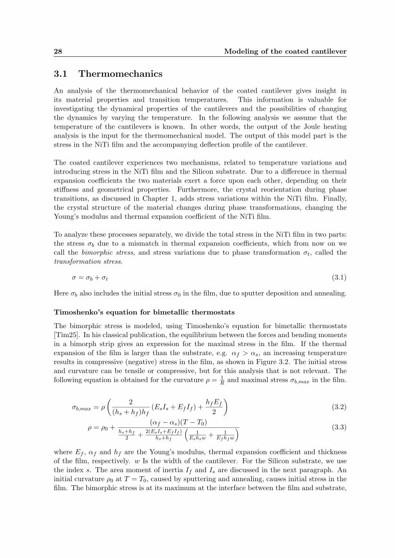
The bimorphic stress is modeled, using Timoshenko’s equation for bimetallic thermostats[Tim25]. In his classical publication, the equilibrium between the forces and bending momentsin a bimorph strip gives an expression for the maximal stress in the film. If the thermalexpansion of the film is larger than the substrate, e.g. αf > αs, an increasing temperatureresults in compressive (negative) stress in the film, as shown in Figure 3.2. The initial stressand curvature can be tensile or compressive, but for this analysis that is not relevant. Thefollowing equation is obtained for the curvature ρ = 1
R and maximal stress σb,max in the film.
σb,max = ρ
(
2
(hs + hf )hf(EsIs + EfIf ) +
hfEf
2
)
(3.2)
ρ = ρ0 +(αf − αs)(T − T0)
hs+hf
2 +2(EsIs+Ef If )
hs+hf
(
1Eshsw + 1
Ef hf w
) (3.3)
where Ef , αf and hf are the Young’s modulus, thermal expansion coefficient and thicknessof the film, respectively. w Is the width of the cantilever. For the Silicon substrate, we usethe index s. The area moment of inertia If and Is are discussed in the next paragraph. Aninitial curvature ρ0 at T = T0, caused by sputtering and annealing, causes initial stress in thefilm. The bimorphic stress is at its maximum at the interface between the film and substrate,
3.1 Thermomechanics 29
R
Pf
Ps
Pf
Ps
NiTi
Si hf
hs
Figure 3.2: Bimorphic bending due to heating along the length of a beam element. R is the radiusof curvature of the cantilever.
where the effect of the thermal mismatch has the largest influence. In further analysis weconsider this interface stress, and replace σb,max by σb.
In Timoshenko’s approach, the assumption is made that the width of the strip is small,compared to its length. Furthermore, it is assumed that the thermal expansion and inertiaremains constant during heating. We extend this analysis to a situation with temperaturedependent stiffness and thermal expansion. As can be seen in (3.3), the stress variesproportional to the temperature. Note that if we assume the film thickness is much lessthan the substrate thickness, (3.3) reduces to Stoney’s equation for the stress in thin films.
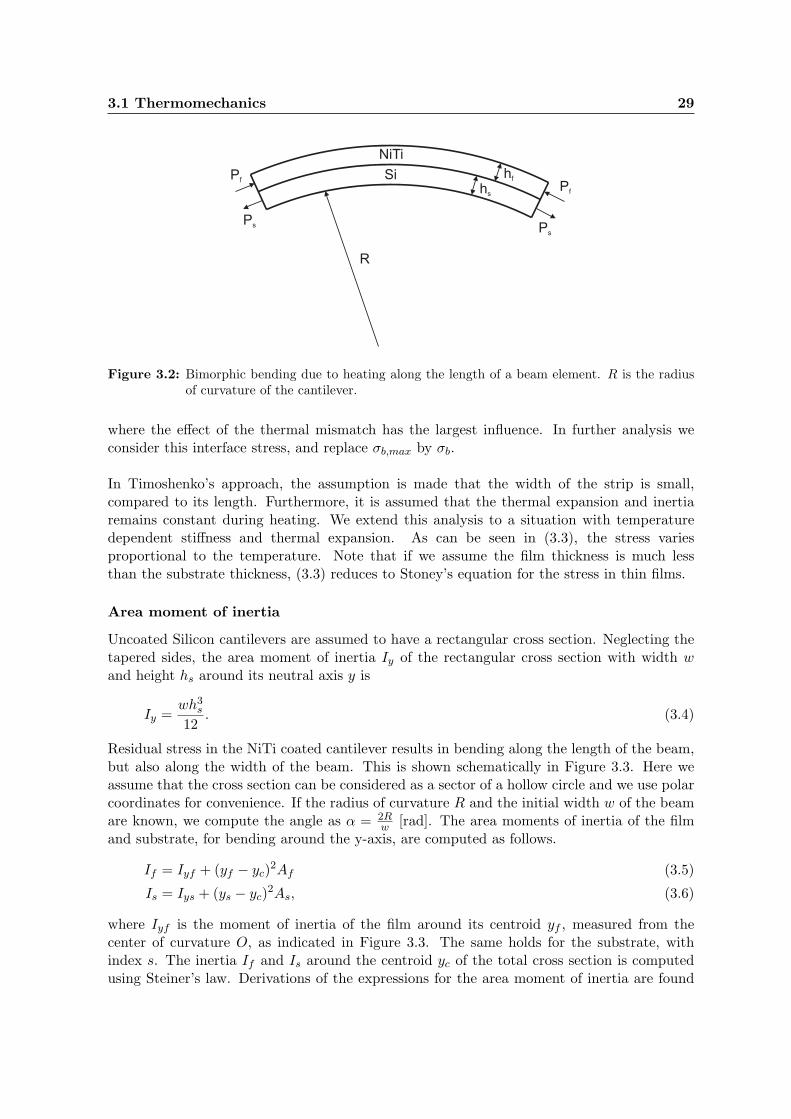
Area moment of inertia
Uncoated Silicon cantilevers are assumed to have a rectangular cross section. Neglecting thetapered sides, the area moment of inertia Iy of the rectangular cross section with width wand height hs around its neutral axis y is
Iy =wh3
s
12. (3.4)
Residual stress in the NiTi coated cantilever results in bending along the length of the beam,but also along the width of the beam. This is shown schematically in Figure 3.3. Here weassume that the cross section can be considered as a sector of a hollow circle and we use polarcoordinates for convenience. If the radius of curvature R and the initial width w of the beamare known, we compute the angle as α = 2R
w [rad]. The area moments of inertia of the filmand substrate, for bending around the y-axis, are computed as follows.
If = Iyf + (yf − yc)2Af (3.5)
Is = Iys + (ys − yc)2As, (3.6)
where Iyf is the moment of inertia of the film around its centroid yf , measured from thecenter of curvature O, as indicated in Figure 3.3. The same holds for the substrate, withindex s. The inertia If and Is around the centroid yc of the total cross section is computedusing Steiner’s law. Derivations of the expressions for the area moment of inertia are found
30 Modeling of the coated cantilever
in Appendix F. The temperature dependence of the moment of inertia lies in a change ofcurvature, due to the thermal mismatch and phase transitions.
R
a
hf
hs
O
yf
yc
ys
Figure 3.3: Dimensions of the NiTi coated cantilever cross section.
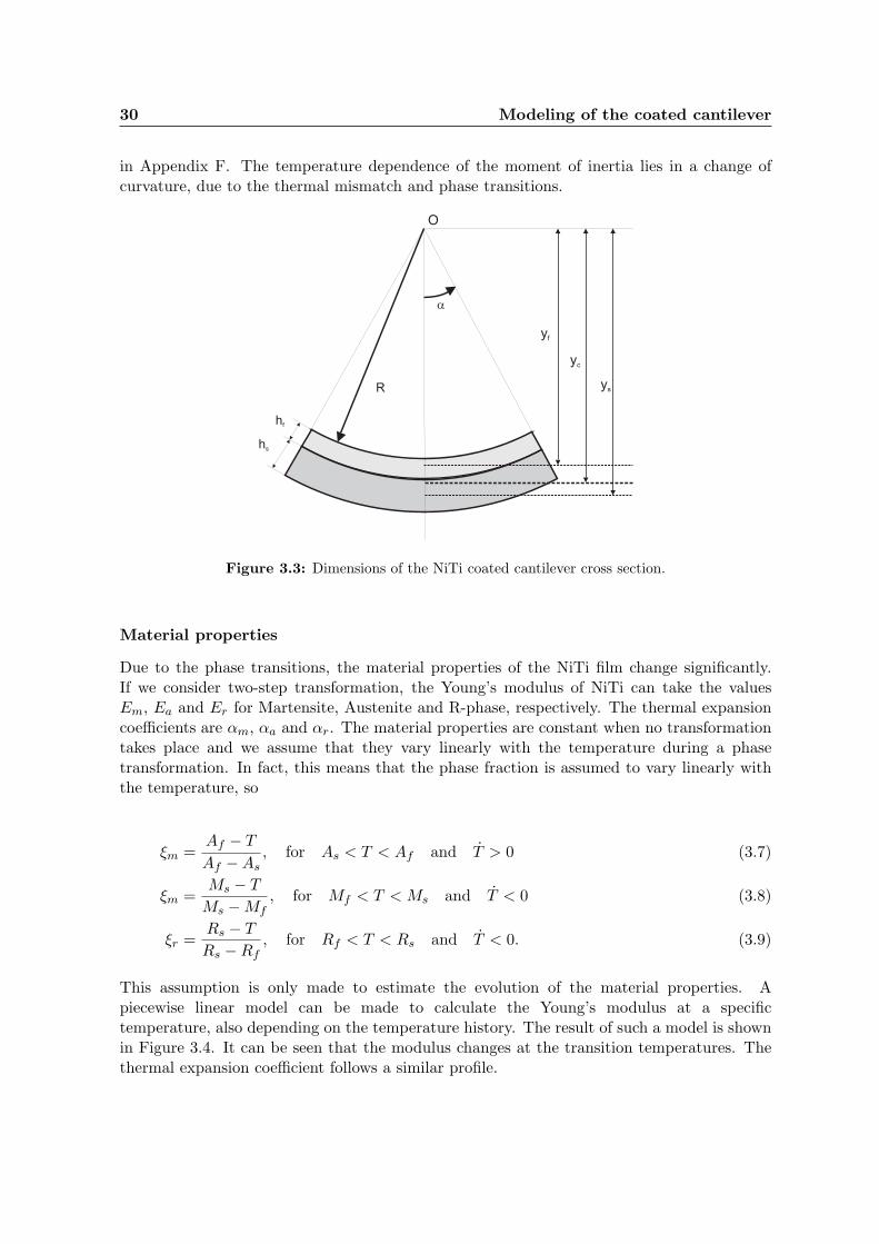
Material properties
Due to the phase transitions, the material properties of the NiTi film change significantly.If we consider two-step transformation, the Young’s modulus of NiTi can take the valuesEm, Ea and Er for Martensite, Austenite and R-phase, respectively. The thermal expansioncoefficients are αm, αa and αr. The material properties are constant when no transformationtakes place and we assume that they vary linearly with the temperature during a phasetransformation. In fact, this means that the phase fraction is assumed to vary linearly withthe temperature, so
ξm =Af − T
Af − As, for As < T < Af and T > 0 (3.7)
ξm =Ms − T
Ms − Mf, for Mf < T < Ms and T < 0 (3.8)
ξr =Rs − T
Rs − Rf, for Rf < T < Rs and T < 0. (3.9)
This assumption is only made to estimate the evolution of the material properties. Apiecewise linear model can be made to calculate the Young’s modulus at a specifictemperature, also depending on the temperature history. The result of such a model is shownin Figure 3.4. It can be seen that the modulus changes at the transition temperatures. Thethermal expansion coefficient follows a similar profile.
3.1 Thermomechanics 31
Temperature [C]
You
ng’
sm
odulu
s[G
Pa]
Ms
Mf As Af
RsRf
Em
Ea
Er
Figure 3.4: Evolution of the Young’s modulus as function of temperature. The solid line indicatesan increasing temperature, the dashed line indicates a decreasing temperature.
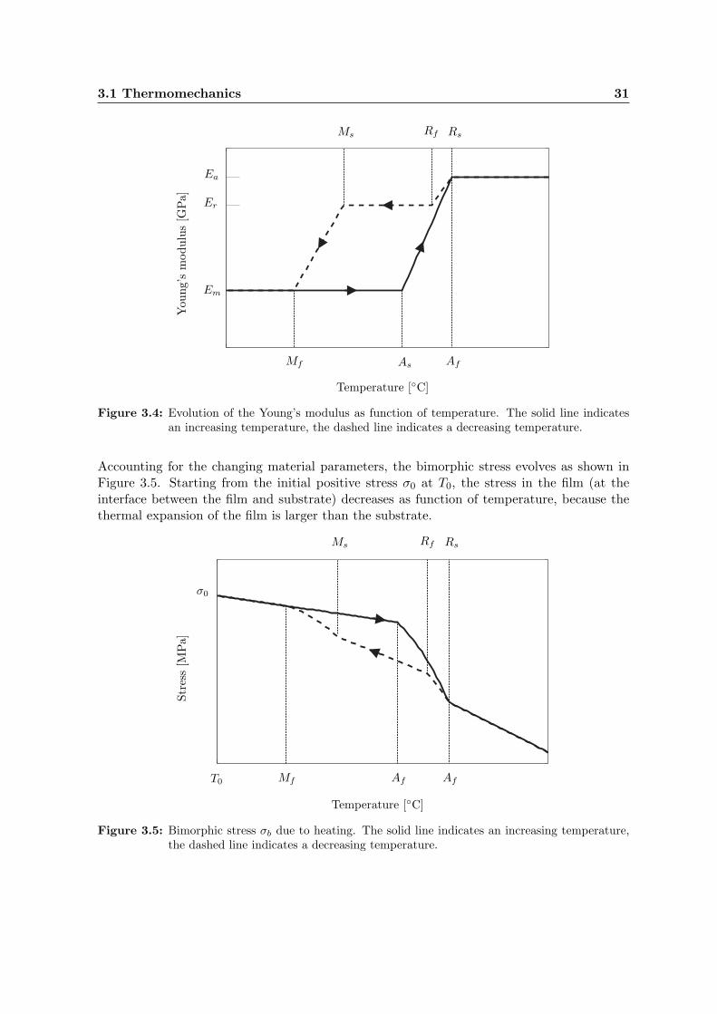
Accounting for the changing material parameters, the bimorphic stress evolves as shown inFigure 3.5. Starting from the initial positive stress σ0 at T0, the stress in the film (at theinterface between the film and substrate) decreases as function of temperature, because thethermal expansion of the film is larger than the substrate.
Temperature [C]
Str
ess
[MPa]
Ms
Mf AfAf
RsRf
σ0
T0
Figure 3.5: Bimorphic stress σb due to heating. The solid line indicates an increasing temperature,the dashed line indicates a decreasing temperature.
32 Modeling of the coated cantilever
3.2 Transformation stress – hysteresis modeling
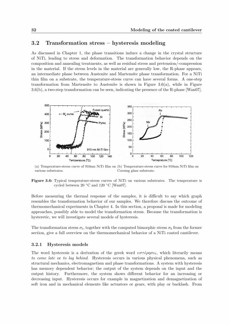
As discussed in Chapter 1, the phase transitions induce a change in the crystal structureof NiTi, leading to stress and deformation. The transformation behavior depends on thecomposition and annealing treatments, as well as residual stress and pretension/-compressionin the material. If the stress levels in the material are generally low, the R-phase appears,an intermediate phase between Austenite and Martensite phase transformation. For a NiTithin film on a substrate, the temperature-stress curve can have several forms. A one-steptransformation from Martensite to Austenite is shown in Figure 3.6(a), while in Figure3.6(b), a two-step transformation can be seen, indicating the presence of the R-phase [Wan07].
(a) Temperature-stress curve of 910nm NiTi film onvarious substrates.
(b) Temperature-stress curve for 910nm NiTi film onCorning glass substrate.
Figure 3.6: Typical temperature-stress curves of NiTi on various substrates. The temperature iscycled between 20 C and 120 C [Wan07].
Before measuring the thermal response of the samples, it is difficult to say which graphresembles the transformation behavior of our samples. We therefore discuss the outcome ofthermomechanical experiments in Chapter 4. In this section, a proposal is made for modelingapproaches, possibly able to model the transformation stress. Because the transformation ishysteretic, we will investigate several models of hysteresis.
The transformation stress σt, together with the computed bimorphic stress σb from the formersection, give a full overview on the thermomechanical behavior of a NiTi coated cantilever.
3.2.1 Hysteresis models
The word hysteresis is a derivation of the greek word υστ ǫρησις, which literarily meansto come late or to lag behind. Hysteresis occurs in various physical phenomena, such asstructural mechanics, electromagnetism and phase transformations. A system with hysteresishas memory dependent behavior; the output of the system depends on the input and theoutput history. Furthermore, the system shows different behavior for an increasing ordecreasing input. Hysteresis occurs for example in magnetization and demagnetization ofsoft iron and in mechanical elements like actuators or gears, with play or backlash. From
3.2 Transformation stress – hysteresis modeling 33
these varying backgrounds in engineering and science, models of hysteresis arised in variousforms.
In general we can subdivide hysteresis models in two classes, physical and geometric models.In physical models, the parameters and their dependence are motivated on the physicalprocesses causing the hysteresis. Geometric models are based on finding equations thatrepresent measured hysteresis curves. The equations have no physical motivation, but simplymap the input on the output as good as possible. In the following paragraphs, existing modelsof hysteresis in shape memory alloys of both classes are reviewed shortly.
Physical models of hysteresis
Ikuta et al. [ITH91] have made a start in modeling the behavior of shape memory alloys,using a variable sublayer approach. The phases of the material are modeled separately andthe total behavior is modeled as a parallel connection of these sublayers of material models.The sublayers consist of basic models of mechanical play in series with a spring. The modelhas some physical motivation, but the actual hysteresis is simply modeled as play. Boydand Lagoudas [BL96] have developed a thermodynamical constitutive model, using the Gibbsfree energy and a dissipation potential. Hardening effects are also incorporated. Bekker andBrinson [BB98] have formulated a model, based on the transformation kinetics of the materialand basic piecewise continuous functions, describing stress and strain relations. The phasefraction in the material is calculated from transformation kinetics. The model is mainlyconcerning about computing the phase fraction as function of temperature.
Mathematical models of hysteresis
Mathematical models of hysteresis exist in various forms. Some are inspired on physicalmodels, but adapted for other applications. We can distinguish models that are a sum ofbasic elements - the hysteresis operators - and differential models. Other geometrical modelsuse the so-called hysteron, a general formulation of hysteresis, applied to some input-ouputbehavior. In all of these three classes models of shape memory alloys are found.
The Preisach model [Pre35] is based on a summation of relay operators with switchingvalues and weight factors. The physical relevance of summing the relay operators is given asbeing the phase transition of separate crystals in an SMA or switching dipoles in magnetichysteresis. Mayergoyz [May91] discusses the model’s properties and limitations extensively.Hughes and Wen [HW97] have worked on Preisach modeling of SMA hysteresis and proposedan identification method.
The Duhem model [MNZ93, OB05] includes a large class of differential models with anextensive amount of properties. The models can be rate-dependent or rate-independent,linear or nonlinear. The motivation for this model is found in electromagnetic charging,where the output changes its behavior when the input changes direction. Derivations ofthe Duhem model are the Bouc-Wen and Madelung model. Dutta et.al. [DGD05, DG05]propose a method to model and control a Shape Memory Alloy wire actuator. The modelis a combination of the Duhem model and Ikuta’s variable sublayer model. It describesJoule heating, phase transformation and stress-strain relations and uses a large amount of
34 Modeling of the coated cantilever
nonlinear curve fits to describe the temperature dependent material parameters.
Macki et.al. [MNZ93] give a general overview of a large amount of mathematical models ofhysteresis. They distinguish between relay hysteresis and active hysteresis. The differencebetween these two is that in the case of active hysteresis, trajectories inside the hysteresisregion (also referred to as the major loop) are possible. The Duhem and Preisach model,as well as some other interesting hysteresis operators are discussed. The ’stop’ operator wasoriginally proposed as a model for plasticity-elasticity. An upper and lower boundary - thestops - are connected by monotone functions. The Krasnosel’skii-Pokrovskii hysteron is ageneralized ’play’ operator. The hysteron can be formulated with any function for the majorloop up and down, and horizontal lines describe the minor loops.
Discussion and model requirements
Constructing a physical model of shape memory alloy hysteresis requires knowledge oftransformation kinetics and energy balance in crystal structures. The parameters describingthese processes are difficult to measure and to interpret. Understanding transformationkinetics and crystal morphology is out the the scope of this project. We therefore focus ongeometrical (or mathematical) models of hysteresis. This conclusion is supported by the workof van der Wijst [Wij98]. He discusses 1D and 3D constitutive models, as proposed in [BL96]and [BB98], as well as geometrical and plasticity based models. The conclusion is thatconstitutive models, based on free energy or transformation kinetics, are very complicated,while still not accurate. Plasticity based models often require measurement of phase fraction,which is difficult and sometimes impossible. He proposes a geometrical model based onconstitutive relations, being a tradeoff between accuracy and simplicity.
Requirements of the model are as follows.
- The phase transformation forms a closed loop, when the material is temperature cycledbetween fully Martensite and fully Austenite phase. This is called the major loop. In fullMartensite or Austenite phase, no transformation takes place anymore. This plateauis called the dead zone. When the major loop is not fully cycled, a so-called minorloop appears. A realistic model has to be able to describe these three mechanisms.Furthermore, the appearance of the R-phase should be modeled if necessary.
- From a control point of view, a simple model would be appealing. A differential model,for example, can easily be included in a control loop and frequency response analysisis relatively easy, making it possible to analyze and control the dynamic behavior ofthe system. A complex model would increase computational effort, possibly addingtime-delay to the system. Other models can eventually be included in a control loopas well, for example as a look-up table or piecewise continuous system. This, however,makes control more complicated.
- The hysteresis in shape memory alloys is rate-independent. This implies that the inputvelocity does not affect the shape or behavior of the output. A physical explanation isfound in the fact that the phase transformation occurs almost instantaneous throughoutthe material and no physical input can reach a higher velocity than the propagation ofthe transformation.
3.2 Transformation stress – hysteresis modeling 35
In the following sections, we will explore the suitability of some mathematical models todescribe the phase transformation hysteresis in SMA. Advantages and disadvantages arediscussed, as well as simulation results. The models are evaluated on the above requirementsand a final decision for modeling the hysteresis in our system is made.
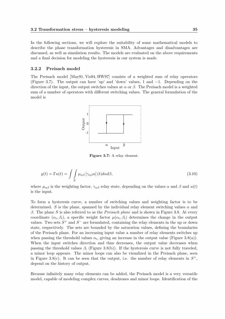
3.2.2 Preisach model
The Preisach model [May91, Vis94, HW97] consists of a weighted sum of relay operators(Figure 3.7). The output can have ’up’ and ’down’ values, 1 and −1. Depending on thedirection of the input, the output switches values at α or β. The Preisach model is a weightedsum of a number of operators with different switching values. The general formulation of themodel is
α β
-1
0
1
Input
Outp
ut
Figure 3.7: A relay element.
y(t) = Γu(t) =
∫ ∫
S
µαβ [γαβu] (t)dαdβ, (3.10)
where µαβ is the weighting factor, γαβ relay state, depending on the values α and β and u(t)is the input.
To form a hysteresis curve, a number of switching values and weighting factor is to bedetermined. S is the plane, spanned by the individual relay element switching values α andβ. The plane S is also referred to as the Preisach plane and is shown in Figure 3.8. At everycoordinate (αi, βi), a specific weight factor µ(αi, βi) determines the change in the outputvalues. Two sets S+ and S− are formulated, containing the relay elements in the up or downstate, respectively. The sets are bounded by the saturation values, defining the boundariesof the Preisach plane. For an increasing input value a number of relay elements switches upwhen passing the threshold values αi, giving an increase in the output value (Figure 3.8(a)).When the input switches direction and thus decreases, the output value decreases whenpassing the threshold values βi (Figure 3.8(b)). If the hysteresis curve is not fully traveled,a minor loop appears. The minor loops can also be visualized in the Preisach plane, seenin Figure 3.8(c). It can be seen that the output, i.e. the number of relay elements in S+,depend on the history of output.
Because infinitely many relay elements can be added, the Preisach model is a very versatilemodel, capable of modeling complex curves, deadzones and minor loops. Identification of the
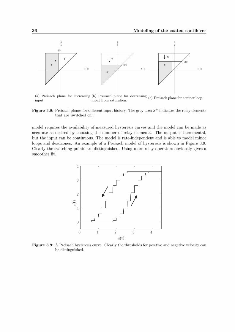
36 Modeling of the coated cantilever
(a) Preisach plane for increasinginput.
(b) Preisach plane for decreasinginput from saturation.
(c) Preisach plane for a minor loop.
Figure 3.8: Preisach planes for different input history. The grey area S+ indicates the relay elementsthat are ’switched on’.
model requires the availability of measured hysteresis curves and the model can be made asaccurate as desired by choosing the number of relay elements. The output is incremental,but the input can be continuous. The model is rate-independent and is able to model minorloops and deadzones. An example of a Preisach model of hysteresis is shown in Figure 3.9.Clearly the switching points are distinguished. Using more relay operators obviously gives asmoother fit.
u(t)
y(t
)
0
0
1
1
2
2
3
3
4
4
Figure 3.9: A Preisach hysteresis curve. Clearly the thresholds for positive and negative velocity canbe distinguished.
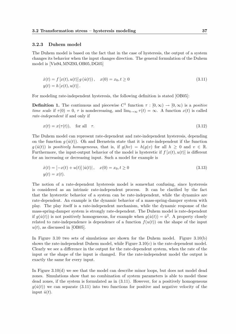
3.2 Transformation stress – hysteresis modeling 37
3.2.3 Duhem model
The Duhem model is based on the fact that in the case of hysteresis, the output of a systemchanges its behavior when the input changes direction. The general formulation of the Duhemmodel is [Vis94,MNZ93,OB05,DG05]
x(t) = f [x(t), u(t)] g (u(t)) , x(0) = x0, t ≥ 0 (3.11)
y(t) = h [x(t), u(t)] .
For modeling rate-independent hysteresis, the following definition is stated [OB05]:
Definition 1. The continuous and piecewise C1 function τ : [0,∞) → [0,∞) is a positivetime scale if τ(0) = 0, τ is nondecreasing, and limt→∞ τ(t) = ∞. A function x(t) is calledrate-independent if and only if
x(t) = x(τ(t)), for all τ. (3.12)
The Duhem model can represent rate-dependent and rate-independent hysteresis, dependingon the function g (u(t)). Oh and Bernstein state that it is rate-independent if the functiong (u(t)) is positively homogeneous, that is, if g(hv) = h(g(v) for all h ≥ 0 and v ∈ R.Furthermore, the input-output behavior of the model is hysteretic if f [x(t), u(t)] is differentfor an increasing or decreasing input. Such a model for example is
x(t) = [−x(t) + u(t)] |u(t)| , x(0) = x0, t ≥ 0 (3.13)
y(t) = x(t).
The notion of a rate-dependent hysteresis model is somewhat confusing, since hysteresisis considered as an intrinsic rate-independent process. It can be clarified by the factthat the hysteretic behavior of a system can be rate-independent, while the dynamics arerate-dependent. An example is the dynamic behavior of a mass-spring-damper system withplay. The play itself is a rate-independent mechanism, while the dynamic response of themass-spring-damper system is strongly rate-dependent. The Duhem model is rate-dependentif g(u(t)) is not positively homogeneous, for example when g(u(t)) = u2. A property closelyrelated to rate-independence is dependence of a function f(u(t)) on the shape of the inputu(t), as discussed in [OB05].
In Figure 3.10 two sets of simulations are shown for the Duhem model. Figure 3.10(b)shows the rate-independent Duhem model, while Figure 3.10(c) is the rate-dependent model.Clearly we see a difference in the output for the rate-dependent system, when the rate of theinput or the shape of the input is changed. For the rate-independent model the output isexactly the same for every input.
In Figure 3.10(d) we see that the model can describe minor loops, but does not model deadzones. Simulations show that no combination of system parameters is able to model thesedead zones, if the system is formulated as in (3.11). However, for a positively homogeneousg(u(t)) we can separate (3.11) into two functions for positive and negative velocity of theinput u(t).
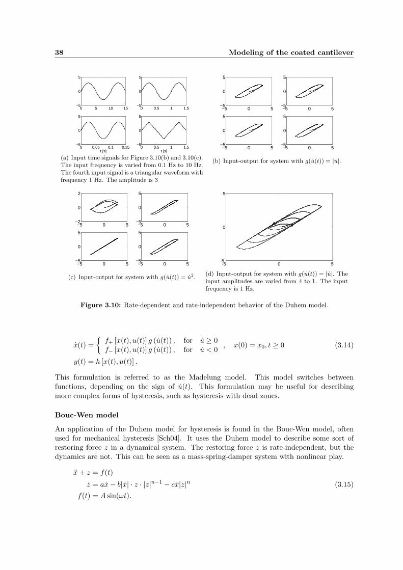
38 Modeling of the coated cantilever
0 5 10 15−5
0
5
0 0.5 1 1.5−5
0
5
0 0.05 0.1 0.15−5
0
5
t [s]0 0.5 1 1.5
−5
0
5
t [s]
(a) Input time signals for Figure 3.10(b) and 3.10(c).The input frequency is varied from 0.1 Hz to 10 Hz.The fourth input signal is a triangular waveform withfrequency 1 Hz. The amplitude is 3
−5 0 5−5
0
5
−5 0 5−5
0
5
−5 0 5−5
0
5
−5 0 5−5
0
5
(b) Input-output for system with g(u(t)) = |u|.
−5 0 5−2
0
2
−5 0 5−5
0
5
−5 0 5−5
0
5
−5 0 5−5
0
5
(c) Input-output for system with g(u(t)) = u2.
-5 0 5-5
0
5
(d) Input-output for system with g(u(t)) = |u|. Theinput amplitudes are varied from 4 to 1. The inputfrequency is 1 Hz.
Figure 3.10: Rate-dependent and rate-independent behavior of the Duhem model.
x(t) =
f+ [x(t), u(t)] g (u(t)) , for u ≥ 0f− [x(t), u(t)] g (u(t)) , for u < 0
, x(0) = x0, t ≥ 0 (3.14)
y(t) = h [x(t), u(t)] .
This formulation is referred to as the Madelung model. This model switches betweenfunctions, depending on the sign of u(t). This formulation may be useful for describingmore complex forms of hysteresis, such as hysteresis with dead zones.
Bouc-Wen model
An application of the Duhem model for hysteresis is found in the Bouc-Wen model, oftenused for mechanical hysteresis [Sch04]. It uses the Duhem model to describe some sort ofrestoring force z in a dynamical system. The restoring force z is rate-independent, but thedynamics are not. This can be seen as a mass-spring-damper system with nonlinear play.
x + z = f(t)
z = ax − b|x| · z · |z|n−1 − cx|z|n (3.15)
f(t) = A sin(ωt).

3.2 Transformation stress – hysteresis modeling 39
The influence of the model’s parameters a, b, c, n and input parameters A and ω on thehysteretic behavior is thoroughly analyzed by Schwanen [Sch04]. Because we are onlyinterested in the hysteretic behavior, only the input-output behavior from x to z is analyzedhere. We thus consider a harmonic input x. The model becomes
z = ax − b|x| · z · |z|n−1 − cx|z|n (3.16)
x(t) = A sin(ωt).
With parameters a = b = c = 1 and n = 2, the hysteresis curve in Figure 3.11 isobtained for varying input amplitude (input frequency is not relevant, since this model israte-independent). We can directly point out big differences with the general Duhem model.First of all, the hysteresis loop is following clockwise. Secondly, the minor loops are different.They don’t increase or decrease along the major loop, but follow a separate trajectory. Thebehavior of the restoring force z differs much from the phase transformation hysteresis curves,seen in Figure 1.5.
x
z
-1
1
0
0-5 5
Figure 3.11: The restoring force z as function of input x with amplitude A = 4, 3, 2, 1.
Identification of the parameters can be a complex procedure. In [Sch04] a two-stepidentification procedure, based on the Levenberg-Marquard algorithm, is used to find theparameters to fit on measurements on a wire rope spring showing mechanical hysteresis.
Another derivation of the Duhem model, directly mapping the input and output on physicalprocesses, describes magnetization in soft iron as a function of a varying magnetic field [OB05,MNZ93].
B(t) = a∣
∣
∣H(t)
∣
∣
∣[bH(t) − B(t)] + cH(t), (3.17)
where the output B(t) is the magnetic flux density as a result of the input magnetic fieldstrength H(t) and a, b and c are positive constants. It can be seen that the model onlyslightly differs from the Bouc-Wen model with n = 1. However, the input-output behaviorchanges significantly, similar to the general Duhem model (3.13).
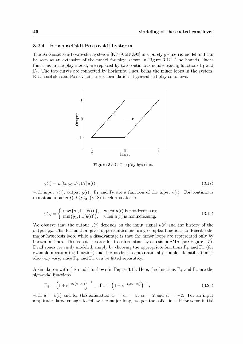
40 Modeling of the coated cantilever
3.2.4 Krasnosel’skii-Pokrovskii hysteron
The Krasnosel’skii-Pokrovskii hysteron [KP89,MNZ93] is a purely geometric model and canbe seen as an extension of the model for play, shown in Figure 3.12. The bounds, linearfunctions in the play model, are replaced by two continuous nondecreasing functions Γ1 andΓ2. The two curves are connected by horizontal lines, being the minor loops in the system.Krasnosel’skii and Pokrovskii state a formulation of generalized play as follows.
Input
Outp
ut
-1
1
0
0-5 5
Figure 3.12: The play hysteron.
y(t) = L [t0, y0; Γ1, Γ2] u(t), (3.18)
with input u(t), output y(t). Γ1 and Γ2 are a function of the input u(t). For continuousmonotone input u(t), t ≥ t0, (3.18) is reformulated to
y(t) =
maxy0, Γ+[u(t)], when u(t) is nondecreasingminy0, Γ−[u(t)], when u(t) is nonincreasing.
(3.19)
We observe that the output y(t) depends on the input signal u(t) and the history of theoutput y0. This formulation gives opportunities for using complex functions to describe themajor hysteresis loop, while a disadvantage is that the minor loops are represented only byhorizontal lines. This is not the case for transformation hysteresis in SMA (see Figure 1.5).Dead zones are easily modeled, simply by choosing the appropriate functions Γ+ and Γ− (forexample a saturating function) and the model is computationally simple. Identification isalso very easy, since Γ+ and Γ− can be fitted separately.
A simulation with this model is shown in Figure 3.13. Here, the functions Γ+ and Γ− are thesigmoidal functions
Γ+ =(
1 + e−a1(u−c1))
−1, Γ− =
(
1 + e−a2(u−c2))
−1, (3.20)
with u = u(t) and for this simulation a1 = a2 = 5, c1 = 2 and c2 = −2. For an inputamplitude, large enough to follow the major loop, we get the solid line. If for some initial
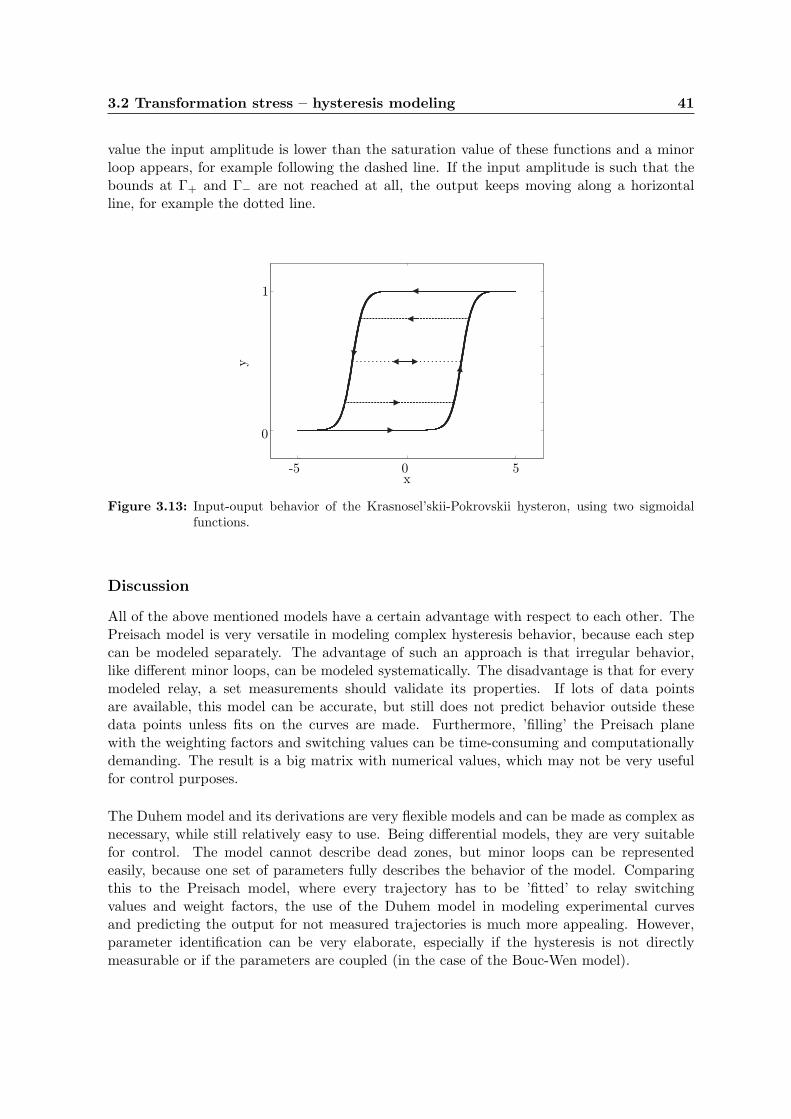
3.2 Transformation stress – hysteresis modeling 41
value the input amplitude is lower than the saturation value of these functions and a minorloop appears, for example following the dashed line. If the input amplitude is such that thebounds at Γ+ and Γ− are not reached at all, the output keeps moving along a horizontalline, for example the dotted line.
x
y
0
0
1
-5 5
Figure 3.13: Input-ouput behavior of the Krasnosel’skii-Pokrovskii hysteron, using two sigmoidalfunctions.
Discussion
All of the above mentioned models have a certain advantage with respect to each other. ThePreisach model is very versatile in modeling complex hysteresis behavior, because each stepcan be modeled separately. The advantage of such an approach is that irregular behavior,like different minor loops, can be modeled systematically. The disadvantage is that for everymodeled relay, a set measurements should validate its properties. If lots of data pointsare available, this model can be accurate, but still does not predict behavior outside thesedata points unless fits on the curves are made. Furthermore, ’filling’ the Preisach planewith the weighting factors and switching values can be time-consuming and computationallydemanding. The result is a big matrix with numerical values, which may not be very usefulfor control purposes.
The Duhem model and its derivations are very flexible models and can be made as complex asnecessary, while still relatively easy to use. Being differential models, they are very suitablefor control. The model cannot describe dead zones, but minor loops can be representedeasily, because one set of parameters fully describes the behavior of the model. Comparingthis to the Preisach model, where every trajectory has to be ’fitted’ to relay switchingvalues and weight factors, the use of the Duhem model in modeling experimental curvesand predicting the output for not measured trajectories is much more appealing. However,parameter identification can be very elaborate, especially if the hysteresis is not directlymeasurable or if the parameters are coupled (in the case of the Bouc-Wen model).

42 Modeling of the coated cantilever
The Krasnosel’skii-Pokrovskii hysteron has an appealing mathematical simplicity and easeof use. It can model the major loop and dead zones without much effort and identificationis straightforward. With well chosen functions Γ1 and Γ2, the model can describe complexbehavior and a least squares fit is sufficient to make an accurate representation of a measuredhysteresis curve. The disadvantage of this model is that the minor loops are representedpoorly. Because the actual measurements determine which model is most suitable to usein our case, we will decide for the best hysteresis model in Chapter 4, where the measuredtemperature-stress curves are presented.
Now that the thermomechanics are discussed, the influence of these processes on the dynamicalbehavior of the system can be analyzed. We therefore present basic equations, describing thedynamics of cantilever beams.
3.3 Dynamics of cantilever beams
If the thermomechanical properties are investigated, we also have access to the rightparameters for investigating the structural dynamics of the system. Having insight in theevolution of the area moment of inertia and the Young’s modulus as function of temperaturegives the opportunity to analyze the vibrations of the cantilevers. The resonance frequenciescan be computed, as well as the damping properties.
Flexural vibrations
The differential equation that describes the free flexural vibrations of a beam is [VZ65]
EIy∂4z(x, t)
∂x4+ ρA
∂2z(x, t)
∂t2= 0, (3.21)
with Young’s modulus E, second moment of area Iy around the y-axis, density ρ and areaA. The vertical displacement z is a function of the position x along the length of the beam,and time t. The solution of this partial differential equation gives the frequency equation andwave equation of the beam. The derivation is found in [VZ65]. The first resonance frequencyof the beam is
ωf =λ2
f
2πL2
√
EI
ρA[Hz], (3.22)
with beam length L and where the wave number λf = 1.87510407 is determined by theboundary conditions.
Because the cantilever in our case is coated with NiTi and the temperature changes both thegeometry and the material properties of the cantilever, (3.22) is of the form
ωf =λ2
f
2πL2
√
E(T )Iy(T )
ρA. (3.23)
The evolution of the Young’s modulus and moment of inertia as function of temperature isfurther discussed in Chapter 4.
3.3 Dynamics of cantilever beams 43
Torsional vibrations
For describing torsional vibrations we find [VZ65]
GK∂2θ(x, t)
∂x2+ ρJp
∂2θ(x, t)
∂t2= 0, (3.24)
with polar moment of inertia Jp, shear modulus G and the torsional stiffness constant K.The resonance frequency is
ωt =λt
2πL
√
GK
ρJp. (3.25)
The polar moment of inertia is the sum of the moment of inertia around the y-axis and z-axis:Jp = Iy + Iz. The wave number for the first torsional resonance is λt = π/2. The torsionalconstant for a sector of a hollow circle is found in [You89]
K =2
3t3Rα, (3.26)
where t is the thickness of the beam, R the radius of curvature of the cross section and αthe angle between the centerline of the curve and the outer point (see Appendix F). Again,temperature dependence lies in the inertial parameters and in the modulus
ωt =λt
2πL
√
G(T )K(T )
ρJp(T ). (3.27)
With these relations as a basis, Finite Element Analysis of the coated cantilever beams canbe done. This is discussed in Chapter 4.
Damping
Structural damping of the cantilever can be investigated both in the time domain and in thefrequency domain. In the time domain, the damping ratio can be deduced from the decay ofamplitude in an impulse time response. This is shown in Figure 3.14(a). If we assume viscousdamping, the amplitude decay Y (t) of the system is exponential:
Y (t) = Y0e−ζωnt, (3.28)
where Y0 is the initial amplitude, ζ is the damping ratio and ωn is the resonance or naturalfrequency. As stated above, the damping can be investigated only if the an impulse responseis available.
In the frequency domain, damping is determined by computing the quality factor Q−1:
Q−1 =f0
f2 − f1, (3.29)
where f0 is the resonance frequency and f2 − f1 is the half power bandwidth. This is thefrequency, at which the power of the oscillation is half the power of the natural frequencyoscillation. In Figure 3.14(b), the frequency response of a single mass-spring-damper system
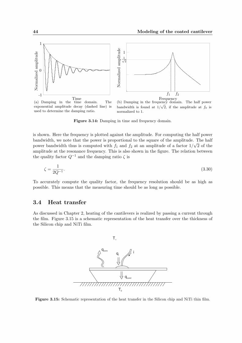
44 Modeling of the coated cantilever
0
1
-1Time
Nor
mal
ized
amplitu
de
(a) Damping in the time domain. Theexponential amplitude decay (dashed line) isused to determine the damping ratio.
Nor
mal
ized
amplitu
de
Frequencyf1 f2
1
1√2
(b) Damping in the frequency domain. The half power
bandwidth is found at 1/√
2, if the amplitude at f0 isnormalized to 1.
Figure 3.14: Damping in time and frequency domain.
is shown. Here the frequency is plotted against the amplitude. For computing the half powerbandwidth, we note that the power is proportional to the square of the amplitude. The halfpower bandwidth thus is computed with f1 and f2 at an amplitude of a factor 1/
√2 of the
amplitude at the resonance frequency. This is also shown in the figure. The relation betweenthe quality factor Q−1 and the damping ratio ζ is
ζ =1
2Q−1. (3.30)
To accurately compute the quality factor, the frequency resolution should be as high aspossible. This means that the measuring time should be as long as possible.
3.4 Heat transfer
As discussed in Chapter 2, heating of the cantilevers is realized by passing a current throughthe film. Figure 3.15 is a schematic representation of the heat transfer over the thickness ofthe Silicon chip and NiTi film.
qconv
qi
qcond
T0
Tµ
i
Figure 3.15: Schematic representation of the heat transfer in the Silicon chip and NiTi thin film.
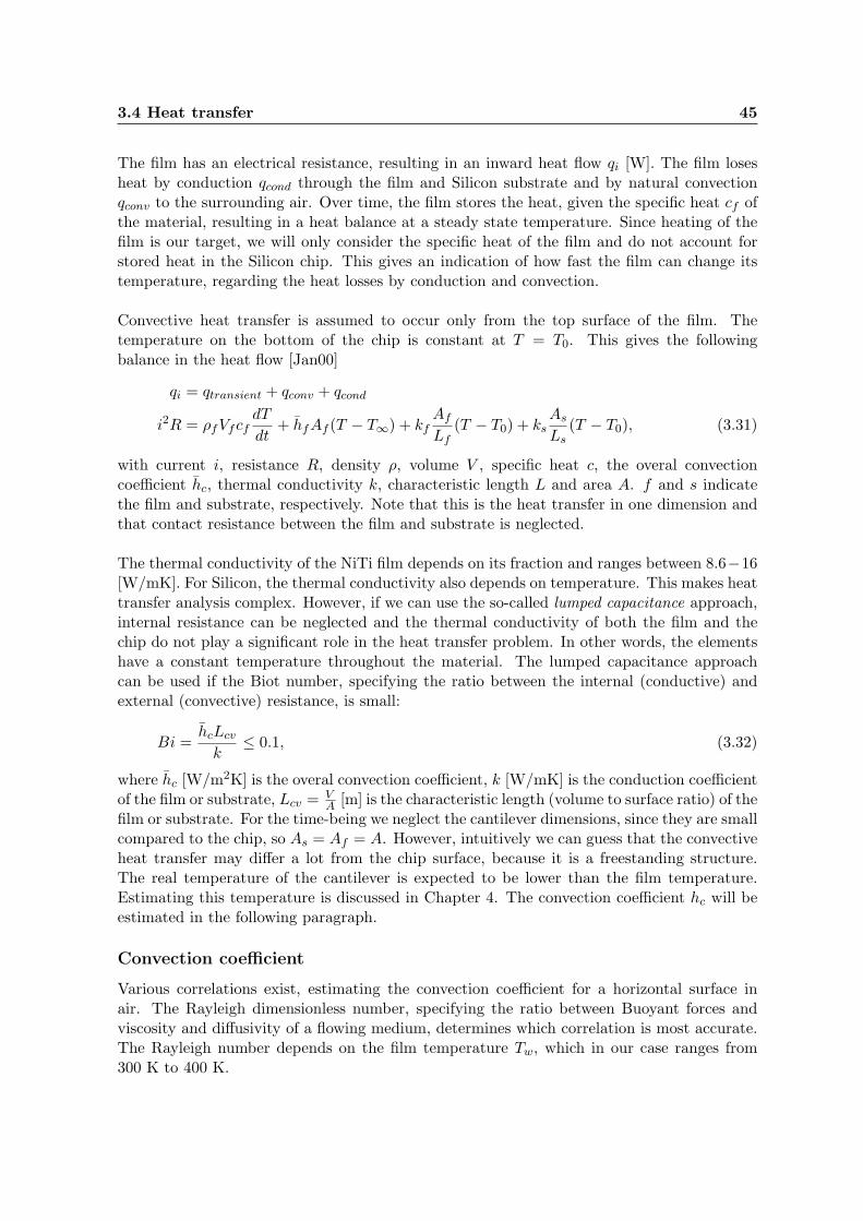
3.4 Heat transfer 45
The film has an electrical resistance, resulting in an inward heat flow qi [W]. The film losesheat by conduction qcond through the film and Silicon substrate and by natural convectionqconv to the surrounding air. Over time, the film stores the heat, given the specific heat cf ofthe material, resulting in a heat balance at a steady state temperature. Since heating of thefilm is our target, we will only consider the specific heat of the film and do not account forstored heat in the Silicon chip. This gives an indication of how fast the film can change itstemperature, regarding the heat losses by conduction and convection.
Convective heat transfer is assumed to occur only from the top surface of the film. Thetemperature on the bottom of the chip is constant at T = T0. This gives the followingbalance in the heat flow [Jan00]
qi = qtransient + qconv + qcond
i2R = ρfVfcfdT
dt+ hfAf (T − T∞) + kf
Af
Lf(T − T0) + ks
As
Ls(T − T0), (3.31)
with current i, resistance R, density ρ, volume V , specific heat c, the overal convectioncoefficient hc, thermal conductivity k, characteristic length L and area A. f and s indicatethe film and substrate, respectively. Note that this is the heat transfer in one dimension andthat contact resistance between the film and substrate is neglected.
The thermal conductivity of the NiTi film depends on its fraction and ranges between 8.6−16[W/mK]. For Silicon, the thermal conductivity also depends on temperature. This makes heattransfer analysis complex. However, if we can use the so-called lumped capacitance approach,internal resistance can be neglected and the thermal conductivity of both the film and thechip do not play a significant role in the heat transfer problem. In other words, the elementshave a constant temperature throughout the material. The lumped capacitance approachcan be used if the Biot number, specifying the ratio between the internal (conductive) andexternal (convective) resistance, is small:
Bi =hcLcv
k≤ 0.1, (3.32)
where hc [W/m2K] is the overal convection coefficient, k [W/mK] is the conduction coefficientof the film or substrate, Lcv = V
A [m] is the characteristic length (volume to surface ratio) of thefilm or substrate. For the time-being we neglect the cantilever dimensions, since they are smallcompared to the chip, so As = Af = A. However, intuitively we can guess that the convectiveheat transfer may differ a lot from the chip surface, because it is a freestanding structure.The real temperature of the cantilever is expected to be lower than the film temperature.Estimating this temperature is discussed in Chapter 4. The convection coefficient hc will beestimated in the following paragraph.
Convection coefficient
Various correlations exist, estimating the convection coefficient for a horizontal surface inair. The Rayleigh dimensionless number, specifying the ratio between Buoyant forces andviscosity and diffusivity of a flowing medium, determines which correlation is most accurate.The Rayleigh number depends on the film temperature Tw, which in our case ranges from300 K to 400 K.
46 Modeling of the coated cantilever
RaLca =gβ
να(Tw − T∞)L3
ca, (3.33)
where Lca is the surface to perimeter ratio, g = 9.81 m/s2 is the gravity constant, β = 1T∞
(for gases), ν is the kinematic viscosity and α is the thermal diffusivity of the surrounding airat Ta = 1
2(T∞ + Tw). The properties of air at specific temperatures are found in [Jan00].Considering the dimensions of the coated Silicon chip and the properties of air at theappropriate temperatures, the Rayleigh dimensionless number varies between 0.003 and 0.06.For these low values, the following correlation is found for the Nusselt number [VDI02], givingthe ratio between convection and conduction in the air.
Nu = 0.766 [Ra · f2(Pr)]1/5 , for Ra · f2(Pr) ≤ 7 · 104, (3.34)
and Pr =ν
α, f2(Pr) =
[
1 +
(
0.322
Pr
)11/20]
−20/11
,
for laminar flow. Here no lower bound is given for the Rayleigh number, so it can be used forany value below 7 · 104. The Nusselt number NuLca is defined as
NuLca =hcLca
kf, (3.35)
where kf is the conductivity of air. It must be equal to (3.34), so the overal convectioncoefficient can be computed from these two equations. This gives h ≈ 10 − 20 W/m2Kfor T = 300 − 400 K. To check if the lumped capacitance approach applies to the problem(3.31), we need and expression for the overal conduction coefficient of the film and substrate.However, if we compute the Biot number both for Silicon and NiTi separately, we can concludethat Bi << 0.01 for both materials and for all relevant temperatures. We can thus neglectthe internal resistance of the film and chip. This reduces (3.31) to a heat balance as functionof time and input current
i2R = ρfVfcfdT
dt+ hcA(T − T∞). (3.36)
This differential equation has a solution of the form
T =B
D+ Ce−Dt, with B =
i2R + hcAT∞
ρfVfcf, D =
hcA
ρfVfcf(3.37)
and integration constant C. Adding a boundary condition T (t = 0) = T0 gives C = T0 − BD .
The thermal time constant τ = 1D =
ρf Vf cf
hcA determines how fast the steady state temperatureis reached, giving an indication of the maximum temperature ’switching’ frequency
fmax =1
2πτ. (3.38)
Assuming constant material properties, as listed in Table 3.1 and a maximum convective heattransfer (so maximum cooling), the upper bound for the switching frequency is 1 Hz. Thisis low, if the cantilever’s temperature is to be actively controlled. However, we must keepin mind that we have now considered heating the complete NiTi film. If the film is heatedlocally, near the cantilever, higher switching rate may be reached.
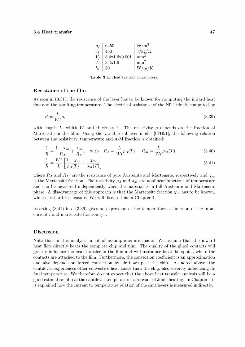
3.4 Heat transfer 47
ρf 6450 kg/m3
cf 460 J/kg/KVf 3.4x1.6x0.001 mm3
A 3.4x1.6 mm2
hc 20 W/m/K
Table 3.1: Heat transfer parameters.
Resistance of the film
As seen in (3.31), the resistance of the layer has to be known for computing the inward heatflux and the resulting temperature. The electrical resistance of the NiTi film is computed by
R =L
Wtρ, (3.39)
with length L, width W and thickness t. The resistivity ρ depends on the fraction ofMartensite in the film. Using the variable sublayer model [ITH91], the following relationbetween the resistivity, temperature and A-M fraction is obtained:
1
R=
1 − χm
RA+
χm
RM, with RA =
L
WtρA(T ), RM =
L
WtρM (T ) (3.40)
1
R=
Wt
L
[
1 − χm
ρA(T )+
χm
ρM (T )
]
, (3.41)
where RA and RM are the resistance of pure Austenite and Martensite, respectively and χm
is the Martensite fraction. The resistivity ρA and ρM are nonlinear functions of temperatureand can be measured independently when the material is in full Austenite and Martensitephase. A disadvantage of this approach is that the Martensite fraction χm has to be known,while it is hard to measure. We will discuss this in Chapter 4.
Inserting (3.41) into (3.36) gives an expression of the temperature as function of the inputcurrent i and martensite fraction χm.
Discussion
Note that in this analysis, a lot of assumptions are made. We assume that the inwardheat flow directly heats the complete chip and film. The quality of the glued contacts willgreatly influence the heat transfer in the film and will introduce local ’hotspots’, where thecontacts are attached to the film. Furthermore, the convection coefficient is an approximationand also depends on forced convection by air flows past the chip. As noted above, thecantilever experiences other convective heat losses than the chip, also severely influencing itsfinal temperature. We therefore do not expect that the above heat transfer analysis will be agood estimation of real the cantilever temperature as a result of Joule heating. In Chapter 4 itis explained how the current to temperature relation of the cantilevers is measured indirectly.

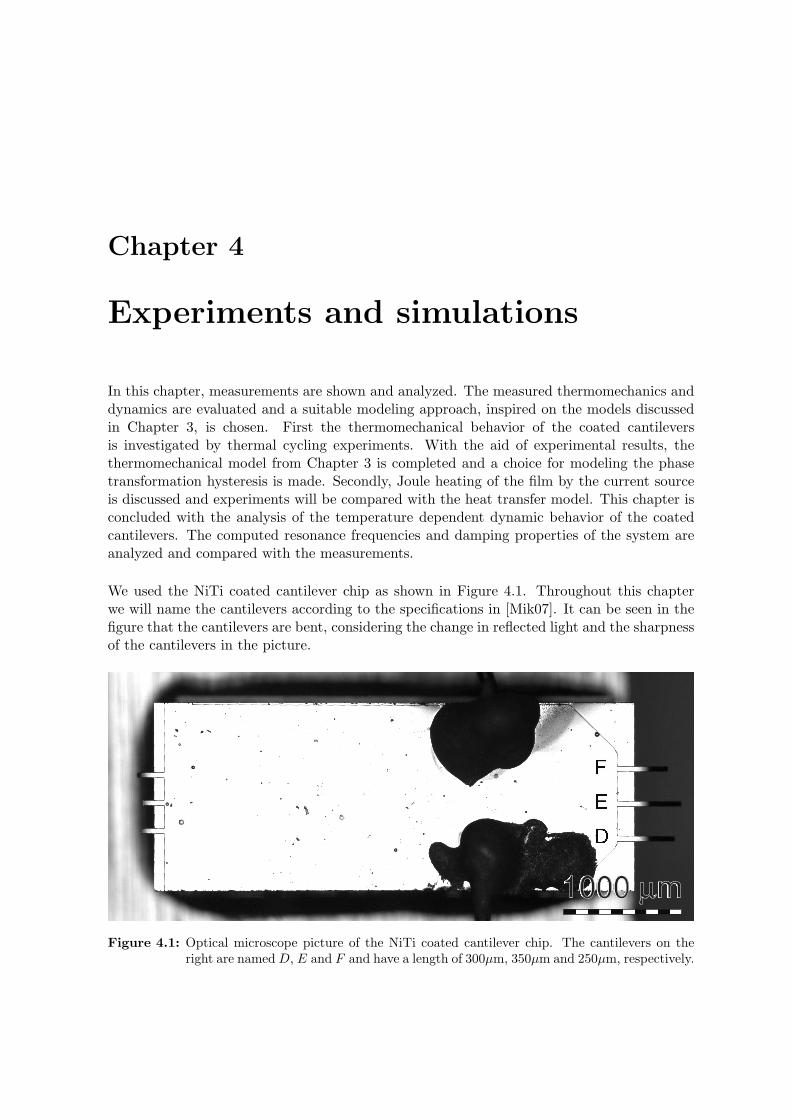
Chapter 4
Experiments and simulations
In this chapter, measurements are shown and analyzed. The measured thermomechanics anddynamics are evaluated and a suitable modeling approach, inspired on the models discussedin Chapter 3, is chosen. First the thermomechanical behavior of the coated cantileversis investigated by thermal cycling experiments. With the aid of experimental results, thethermomechanical model from Chapter 3 is completed and a choice for modeling the phasetransformation hysteresis is made. Secondly, Joule heating of the film by the current sourceis discussed and experiments will be compared with the heat transfer model. This chapter isconcluded with the analysis of the temperature dependent dynamic behavior of the coatedcantilevers. The computed resonance frequencies and damping properties of the system areanalyzed and compared with the measurements.
We used the NiTi coated cantilever chip as shown in Figure 4.1. Throughout this chapterwe will name the cantilevers according to the specifications in [Mik07]. It can be seen in thefigure that the cantilevers are bent, considering the change in reflected light and the sharpnessof the cantilevers in the picture.
1000 mµ
Figure 4.1: Optical microscope picture of the NiTi coated cantilever chip. The cantilevers on theright are named D, E and F and have a length of 300µm, 350µm and 250µm, respectively.
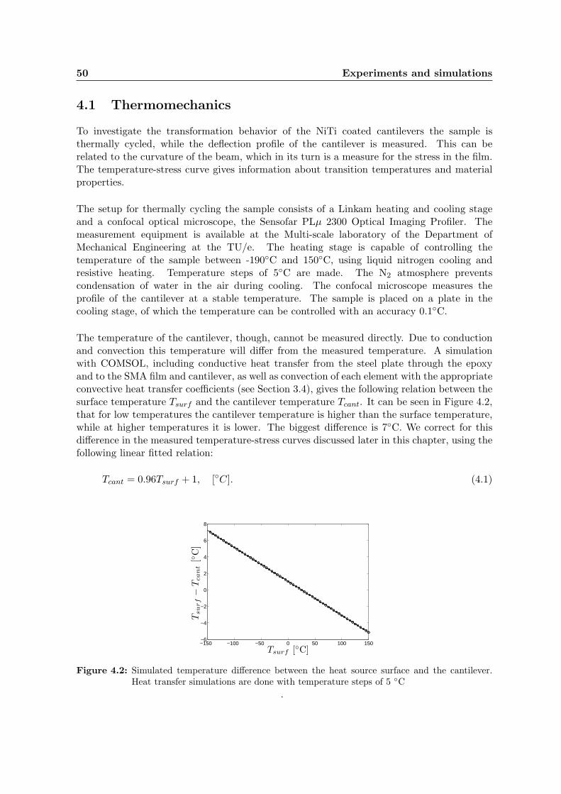
50 Experiments and simulations
4.1 Thermomechanics
To investigate the transformation behavior of the NiTi coated cantilevers the sample isthermally cycled, while the deflection profile of the cantilever is measured. This can berelated to the curvature of the beam, which in its turn is a measure for the stress in the film.The temperature-stress curve gives information about transition temperatures and materialproperties.
The setup for thermally cycling the sample consists of a Linkam heating and cooling stageand a confocal optical microscope, the Sensofar PLµ 2300 Optical Imaging Profiler. Themeasurement equipment is available at the Multi-scale laboratory of the Department ofMechanical Engineering at the TU/e. The heating stage is capable of controlling thetemperature of the sample between -190C and 150C, using liquid nitrogen cooling andresistive heating. Temperature steps of 5C are made. The N2 atmosphere preventscondensation of water in the air during cooling. The confocal microscope measures theprofile of the cantilever at a stable temperature. The sample is placed on a plate in thecooling stage, of which the temperature can be controlled with an accuracy 0.1C.
The temperature of the cantilever, though, cannot be measured directly. Due to conductionand convection this temperature will differ from the measured temperature. A simulationwith COMSOL, including conductive heat transfer from the steel plate through the epoxyand to the SMA film and cantilever, as well as convection of each element with the appropriateconvective heat transfer coefficients (see Section 3.4), gives the following relation between thesurface temperature Tsurf and the cantilever temperature Tcant. It can be seen in Figure 4.2,that for low temperatures the cantilever temperature is higher than the surface temperature,while at higher temperatures it is lower. The biggest difference is 7C. We correct for thisdifference in the measured temperature-stress curves discussed later in this chapter, using thefollowing linear fitted relation:
Tcant = 0.96Tsurf + 1, [C]. (4.1)
−150 −100 −50 0 50 100 150−6
−4
−2
0
2
4
6
8
Tsurf [C]
Tsu
rf−
Tcan
t[
C]
Figure 4.2: Simulated temperature difference between the heat source surface and the cantilever.Heat transfer simulations are done with temperature steps of 5 C
.
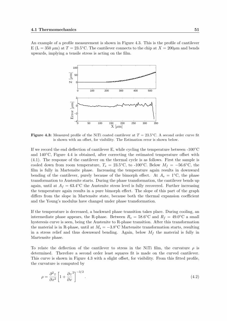
4.1 Thermomechanics 51
An example of a profile measurement is shown in Figure 4.3. This is the profile of cantileverE (L = 350 µm) at T = 23.5C. The cantilever connects to the chip at X = 200µm and bendsupwards, implying a tensile stress is acting on the film.
0 100 200 300 400 500
0
50
100
0 50 100 150 200 250 300 350−4
−2
0
2
X [µm]
Z[µ
m]
Err
or[µ
m]
Figure 4.3: Measured profile of the NiTi coated cantilever at T = 23.5C. A second order curve fitis shown with an offset, for visibility. The Estimation error is shown below.
If we record the end deflection of cantilever E, while cycling the temperature between -100Cand 140C, Figure 4.4 is obtained, after correcting the estimated temperature offset with(4.1). The response of the cantilever on the thermal cycle is as follows. First the sample iscooled down from room temperature, Ts = 23.5C, to -100C. Below Mf = −56.6C, thefilm is fully in Martensite phase. Increasing the temperature again results in downwardbending of the cantilever, purely because of the bimorph effect. At As = 1C, the phasetransformation to Austenite starts. During the phase transformation, the cantilever bends upagain, until at Af = 63.4C the Austenite stress level is fully recovered. Further increasingthe temperature again results in a pure bimorph effect. The slope of this part of the graphdiffers from the slope in Martensite state, because both the thermal expansion coefficientand the Young’s modulus have changed under phase transformation.
If the temperature is decreased, a backward phase transition takes place. During cooling, anintermediate phase appears, the R-phase. Between Rs = 58.6C and Rf = 49.0C a smallhysteresis curve is seen, being the Austenite to R-phase transition. After this transformationthe material is in R-phase, until at Ms = −3.8C Martensite transformation starts, resultingin a stress relief and thus downward bending. Again, below Mf the material is fully inMartensite phase.
To relate the deflection of the cantilever to stress in the NiTi film, the curvature ρ isdetermined. Therefore a second order least squares fit is made on the curved cantilever.This curve is shown in Figure 4.3 with a slight offset, for visibility. From this fitted profile,the curvature is computed by
ρ =∂2z
∂x2
[
1 +∂z
∂x
2]−3/2
. (4.2)
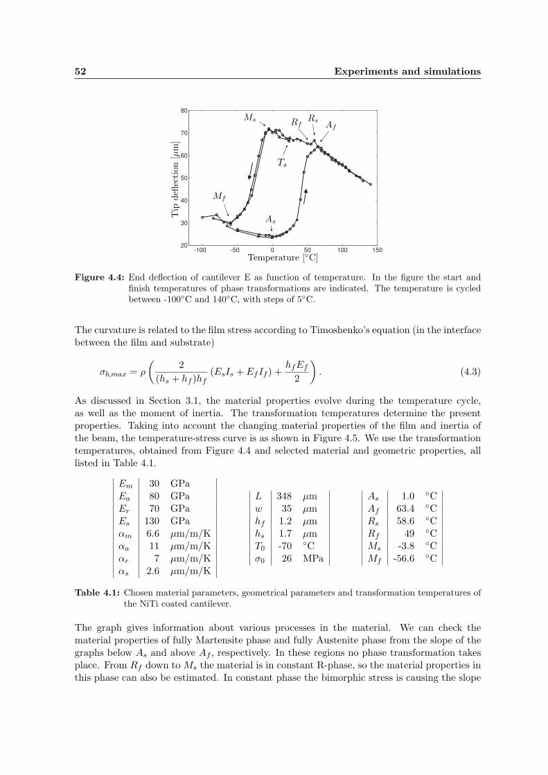
52 Experiments and simulations
-100 -50 0 50 100 15020
30
40
50
60
70
80
Temperature [C]
Tip
defl
ecti
on[µ
m]
Ms
Mf
As
Af
RsRf
Ts
Figure 4.4: End deflection of cantilever E as function of temperature. In the figure the start andfinish temperatures of phase transformations are indicated. The temperature is cycledbetween -100C and 140C, with steps of 5C.
The curvature is related to the film stress according to Timoshenko’s equation (in the interfacebetween the film and substrate)
σb,max = ρ
(
2
(hs + hf )hf(EsIs + EfIf ) +
hfEf
2
)
. (4.3)
As discussed in Section 3.1, the material properties evolve during the temperature cycle,as well as the moment of inertia. The transformation temperatures determine the presentproperties. Taking into account the changing material properties of the film and inertia ofthe beam, the temperature-stress curve is as shown in Figure 4.5. We use the transformationtemperatures, obtained from Figure 4.4 and selected material and geometric properties, alllisted in Table 4.1.
Em 30 GPaEa 80 GPaEr 70 GPaEs 130 GPaαm 6.6 µm/m/Kαa 11 µm/m/Kαr 7 µm/m/Kαs 2.6 µm/m/K
L 348 µmw 35 µmhf 1.2 µmhs 1.7 µmT0 -70 Cσ0 26 MPa
As 1.0 CAf 63.4 CRs 58.6 CRf 49 CMs -3.8 CMf -56.6 C
Table 4.1: Chosen material parameters, geometrical parameters and transformation temperatures ofthe NiTi coated cantilever.
The graph gives information about various processes in the material. We can check thematerial properties of fully Martensite phase and fully Austenite phase from the slope of thegraphs below As and above Af , respectively. In these regions no phase transformation takesplace. From Rf down to Ms the material is in constant R-phase, so the material properties inthis phase can also be estimated. In constant phase the bimorphic stress is causing the slope
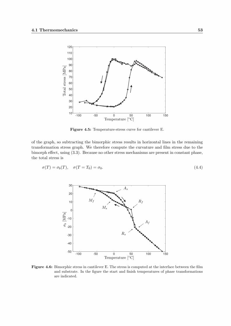
4.1 Thermomechanics 53
-100 -50 0 50 100 15010
20
30
40
50
60
70
80
90
100
110
120
Temperature [C]
Tot
alst
ress
[MPa]
Figure 4.5: Temperature-stress curve for cantilever E.
of the graph, so subtracting the bimorphic stress results in horizontal lines in the remainingtransformation stress graph. We therefore compute the curvature and film stress due to thebimorph effect, using (3.3). Because no other stress mechanisms are present in constant phase,the total stress is
σ(T ) = σb(T ), σ(T = T0) = σ0. (4.4)
-100 -50 0 50 100 150-50
-40
-30
-20
-10
0
10
20
30
Temperature [C]
σb
[MPa]
Ms
Mf
As
Af
Rs
Rf
Figure 4.6: Bimorphic stress in cantilever E. The stress is computed at the interface between the filmand substrate. In the figure the start and finish temperatures of phase transformationsare indicated.
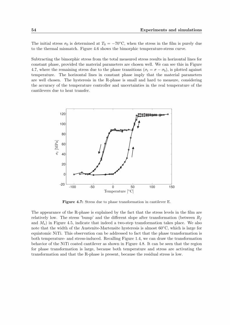
54 Experiments and simulations
The initial stress σ0 is determined at T0 = −70C, when the stress in the film is purely dueto the thermal mismatch. Figure 4.6 shows the bimorphic temperature-stress curve.
Subtracting the bimorphic stress from the total measured stress results in horizontal lines forconstant phase, provided the material parameters are chosen well. We can see this in Figure4.7, where the remaining stress due to the phase transitions (σt = σ − σb), is plotted againsttemperature. The horizontal lines in constant phase imply that the material parametersare well chosen. The hysteresis in the R-phase is small and hard to measure, consideringthe accuracy of the temperature controller and uncertainties in the real temperature of thecantilevers due to heat transfer.
-100 -50 0 50 100 150-20
0
20
40
60
80
100
120
Temperature [C]
σt
[MPa]
Figure 4.7: Stress due to phase transformation in cantilever E.
The appearance of the R-phase is explained by the fact that the stress levels in the film arerelatively low. The stress ’bump’ and the different slope after transformation (between Rf
and Ms) in Figure 4.5, indicate that indeed a two-step transformation takes place. We alsonote that the width of the Austenite-Martensite hysteresis is almost 60C, which is large forequiatomic NiTi. This observation can be addressed to fact that the phase transformation isboth temperature- and stress-induced. Recalling Figure 1.4, we can draw the transformationbehavior of the NiTi coated cantilever as shown in Figure 4.8. It can be seen that the regionfor phase transformation is large, because both temperature and stress are activating thetransformation and that the R-phase is present, because the residual stress is low.
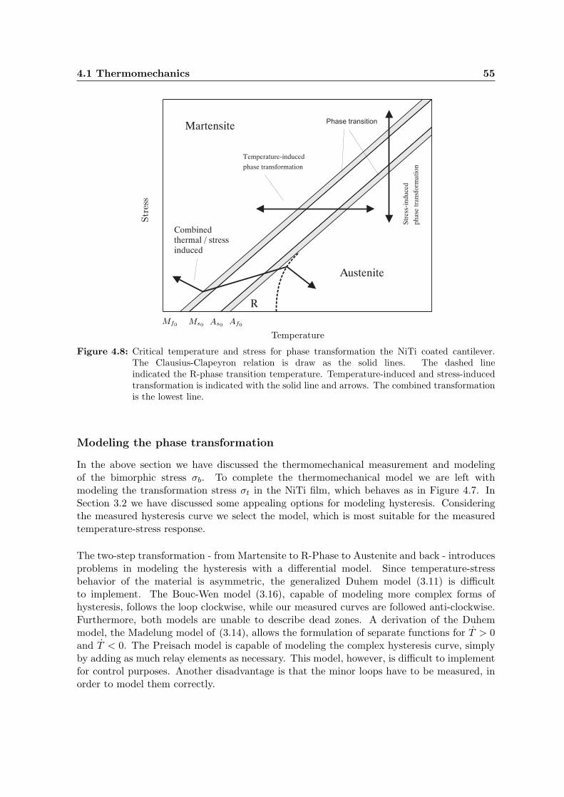
4.1 Thermomechanics 55
Austenite
Martensite
R
Str
ess-
ind
uce
d
ph
ase
tran
sfo
rmat
ion
Temperature-induced
phase transformation
Combinedthermal / stressinduced
Phase transition
Temperature
Str
ess
As0Af0
Ms0Mf0
Figure 4.8: Critical temperature and stress for phase transformation the NiTi coated cantilever.The Clausius-Clapeyron relation is draw as the solid lines. The dashed lineindicated the R-phase transition temperature. Temperature-induced and stress-inducedtransformation is indicated with the solid line and arrows. The combined transformationis the lowest line.
Modeling the phase transformation
In the above section we have discussed the thermomechanical measurement and modelingof the bimorphic stress σb. To complete the thermomechanical model we are left withmodeling the transformation stress σt in the NiTi film, which behaves as in Figure 4.7. InSection 3.2 we have discussed some appealing options for modeling hysteresis. Consideringthe measured hysteresis curve we select the model, which is most suitable for the measuredtemperature-stress response.
The two-step transformation - from Martensite to R-Phase to Austenite and back - introducesproblems in modeling the hysteresis with a differential model. Since temperature-stressbehavior of the material is asymmetric, the generalized Duhem model (3.11) is difficultto implement. The Bouc-Wen model (3.16), capable of modeling more complex forms ofhysteresis, follows the loop clockwise, while our measured curves are followed anti-clockwise.Furthermore, both models are unable to describe dead zones. A derivation of the Duhemmodel, the Madelung model of (3.14), allows the formulation of separate functions for T > 0and T < 0. The Preisach model is capable of modeling the complex hysteresis curve, simplyby adding as much relay elements as necessary. This model, however, is difficult to implementfor control purposes. Another disadvantage is that the minor loops have to be measured, inorder to model them correctly.

56 Experiments and simulations
The Krasnosel’skii-Pokrovskii hysteron is a good choice to model this hysteresis curve. Atfirst sight, this model has some similarities with the Madelung model, though the hysteronis not a differential model. This makes it possible to make a least squares fit simply onthe measured hysteresis loop, while the Madelung model requires more a sophisticatedidentification procedure. Although the minor loops are simply represented by horizontallines, we still approach the behavior of the material well in accordance with the minor loops,as shown qualitatively in Figure 1.5. Only on approaching the major loop, a significantdifference is expected between the measured and modeled curves.
Since the major loop shows saturation behavior in both the A-R transformation and the R-Mtransformation (the dead zones), it is evident that using saturation functions for T ≥ 0 andT ≤ 0 could give good results. Recalling the formulation of the Krasnosel’skii-Pokrovskiihysteron, we define the transformation stress as
σt(T ) =
maxσt,0, Γ+[T ], when T is nondecreasingminσt,0, Γ−[T ], when T is nonincreasing
, (4.5)
where σt,0 is the stress history variable and
Γ+(T ) = S(T, p1) (4.6)
Γ−(T ) = S(T, p2) + S(T, p
3) (4.7)
S(T, pi) = pi1 + pi2
(
1 + epi3(T−pi4))
−1, i = 1, 2, 3. (4.8)
Here we use one sigmoidal function for a nondecreasing input and the sum of two sigmoidalsfor a nonincreasing input. The function S(T, p
i) requires four parameters, so the total model
has 12 parameters, to be fitted on the measured data. We therefore divide the major loopinto three intervals, where the sigmoidal functions are fitted:
S(T, p1), for T > 0 (4.9)
S(T, p2), for T < 0 and T < Rf (4.10)
S(T, p3), for T < 0 and T > Ms. (4.11)
The results of the identification procedure are shown in Figure 4.9. The error stays within 5MPa, except at the R-phase transitions, where the slope of the graph changes abruptly, andthus the function fails to fit well over the data. A simulation with the model for an inputof changing amplitude gives Figure 4.10. Clearly we see the minor loops appear when theamplitude decreases.
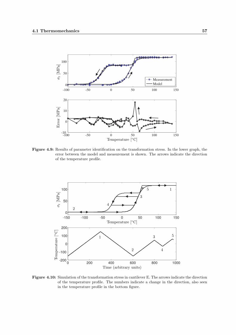
4.1 Thermomechanics 57
-100 -50 0 50 100 150
0
50
100
Measurement
Model
-100 -50 0 50 100 150-10
0
10
20
Temperature [C]
σt
[MPa]
Err
or[M
Pa]
Figure 4.9: Results of parameter identification on the transformation stress. In the lower graph, theerror between the model and measurement is shown. The arrows indicate the directionof the temperature profile.
-150 -100 -50 0 50 100 150
0
50
100
0 200 400 600 800 1000-200
-100
0
100
200
1
1
2
2
3
3
4
4
5
5
Temperature [C]
σt
[MPa]
Time (arbitrary units)
Tem
per
ature
[C
]
Figure 4.10: Simulation of the transformation stress in cantilever E. The arrows indicate the directionof the temperature profile. The numbers indicate a change in the direction, also seenin the temperature profile in the bottom figure.
58 Experiments and simulations
Discussion
We have formulated a thermomechanical model, fully capable of describing thetemperature-stress behavior of the NiTi coated cantilever. The stress is computed atthe interface between the film and substrate, where the bimorphic stress σb is at itsmaximum. The model is based on physical information for the bimorphic stress, while thetransformation stress is a geometrical model.
Now we have fully analyzed the thermomechanical behavior at controlled environment, ananalysis of the influence of the thermomechanics on the dynamics of the system can be done.We therefore heat the cantilever not with the N2 heating and cooling stage, but with thecurrent source. The next section discusses measurements with the current source, to obtainrelation between the induced current and the resulting temperature of the cantilever.
4.2 Joule heating
In Chapter 2 it is explained how Joule heating of the cantilever chip is realized by attachingtwo wires to the chip, using conductive glue. A current source supplies a constant current,while the resistance of the film changes under varying temperature. In Chapter 3, a 1Dmodel of the heat transfer and a model of the resistance of the NiTi film is formulated.The heat transfer coefficient is estimated and the resistivity is computed, using the phasefraction.
As discussed in Chapter 2, the wire bonds are made with conductive glue, which is an epoxywith silver particles. A lot of uncertainties arise when measuring the resistance of the film.If the voltage is measured at a certain current input, the resistance of the glue, as well ascontact resistance between the glue and the NiTi surface, is measured. Furthermore, theepoxy could have some trapped air in between, resulting in a capacitive effect. Resistancemeasurements give rise to problems, severely increasing the complexity of the heat transferproblem. The resistance measurements are not reproducible and even fluctuate severely at aconstant current, due to air flows and unpredictable behavior of the glue.
Because the thermal response of the cantilever to an induced current cannot be measureddirectly, an indirect measurement approach has to be followed. This approach is to measurethe deflection profile of the cantilever when heating and cooling with a calibrated heatingsource and to repeat the measurement with the current source. The temperature-stressresponse for the calibrated heat source is compared with the current source measurement,which should be similar in the same temperature range.
The measured current-stress curves are compared to the temperature-stress curves in Figure4.11. The slope of the current-stress curve is not linear, since Joule heating is not proportionalto the input current. Heating from room temperature, we distinguish the R-phase transitionin both graphs, indicating that at around 250 mA, the cantilevers are at a temperatureof 60 C. However, repeating the measurements did not give reproducible results, becauseof the fluctuating resistance of the system. Where therefore can not accurately estimatethe relation between the induced current and the cantilever temperature. Wirebonding thecontacts would give a better quality bond, but to do so, the surface quality must be better
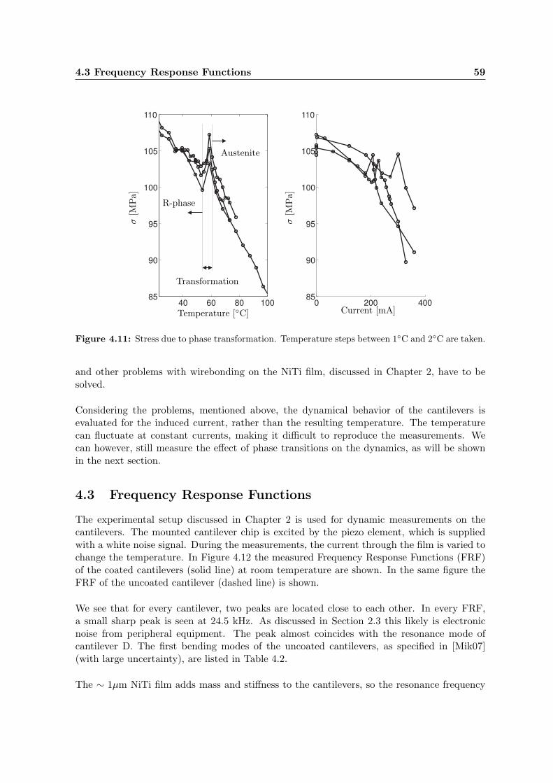
4.3 Frequency Response Functions 59
40 60 80 10085
90
95
100
105
110
0 200 40085
90
95
100
105
110
Temperature [C]
σ[M
Pa]
σ[M
Pa]
Current [mA]
Austenite
R-phase
Transformation
Figure 4.11: Stress due to phase transformation. Temperature steps between 1C and 2C are taken.
and other problems with wirebonding on the NiTi film, discussed in Chapter 2, have to besolved.
Considering the problems, mentioned above, the dynamical behavior of the cantilevers isevaluated for the induced current, rather than the resulting temperature. The temperaturecan fluctuate at constant currents, making it difficult to reproduce the measurements. Wecan however, still measure the effect of phase transitions on the dynamics, as will be shownin the next section.
4.3 Frequency Response Functions
The experimental setup discussed in Chapter 2 is used for dynamic measurements on thecantilevers. The mounted cantilever chip is excited by the piezo element, which is suppliedwith a white noise signal. During the measurements, the current through the film is varied tochange the temperature. In Figure 4.12 the measured Frequency Response Functions (FRF)of the coated cantilevers (solid line) at room temperature are shown. In the same figure theFRF of the uncoated cantilever (dashed line) is shown.
We see that for every cantilever, two peaks are located close to each other. In every FRF,a small sharp peak is seen at 24.5 kHz. As discussed in Section 2.3 this likely is electronicnoise from peripheral equipment. The peak almost coincides with the resonance mode ofcantilever D. The first bending modes of the uncoated cantilevers, as specified in [Mik07](with large uncertainty), are listed in Table 4.2.
The ∼ 1µm NiTi film adds mass and stiffness to the cantilevers, so the resonance frequency
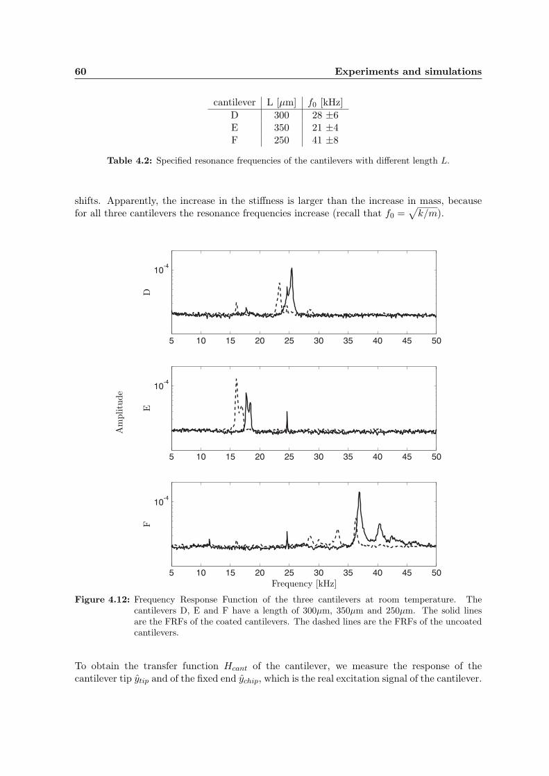
60 Experiments and simulations
cantilever L [µm] f0 [kHz]
D 300 28 ±6E 350 21 ±4F 250 41 ±8
Table 4.2: Specified resonance frequencies of the cantilevers with different length L.
shifts. Apparently, the increase in the stiffness is larger than the increase in mass, becausefor all three cantilevers the resonance frequencies increase (recall that f0 =
√
k/m).
5 10 15 20 25 30 35 40 45 50
10-4
5 10 15 20 25 30 35 40 45 50
10-4
5 10 15 20 25 30 35 40 45 50
10-4
Frequency [kHz]
Am
plitu
de
DE
F
Figure 4.12: Frequency Response Function of the three cantilevers at room temperature. Thecantilevers D, E and F have a length of 300µm, 350µm and 250µm. The solid linesare the FRFs of the coated cantilevers. The dashed lines are the FRFs of the uncoatedcantilevers.
To obtain the transfer function Hcant of the cantilever, we measure the response of thecantilever tip ytip and of the fixed end ychip, which is the real excitation signal of the cantilever.
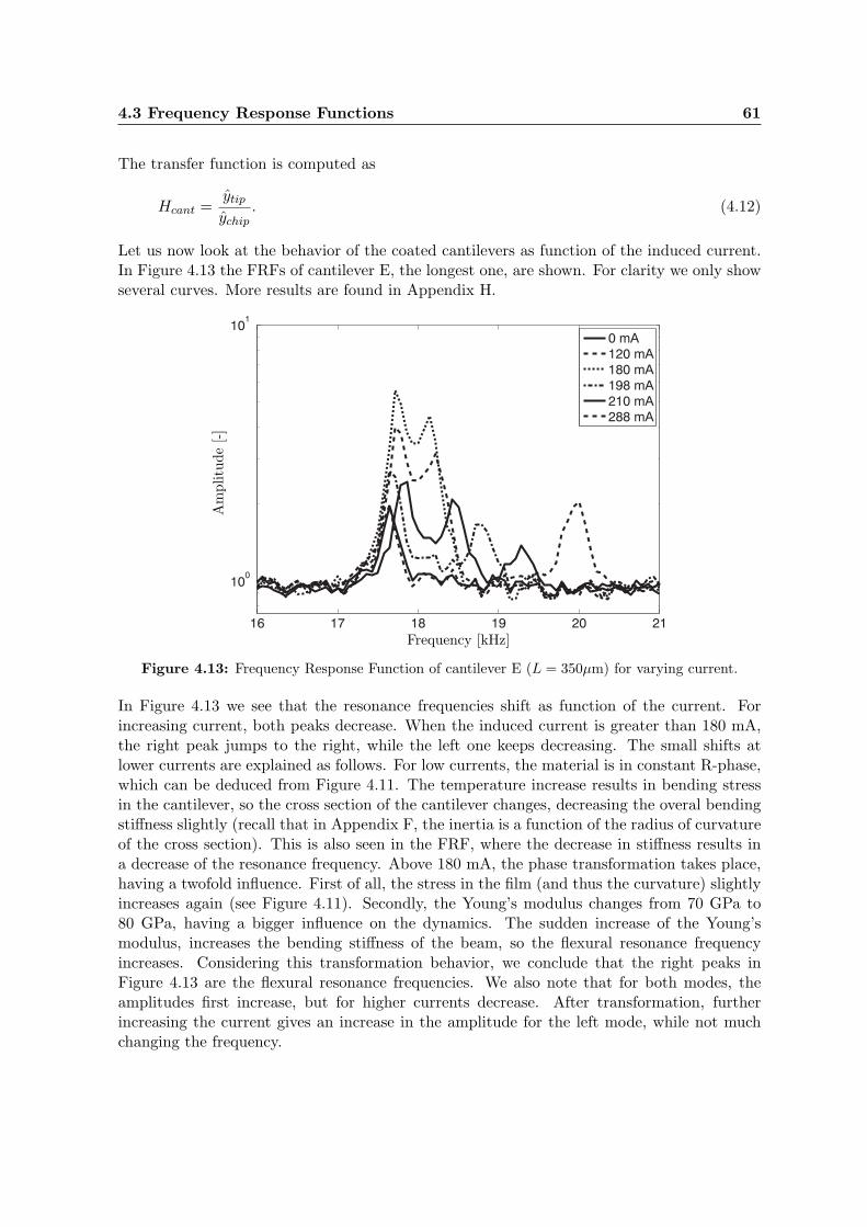
4.3 Frequency Response Functions 61
The transfer function is computed as
Hcant =ytip
ychip. (4.12)
Let us now look at the behavior of the coated cantilevers as function of the induced current.In Figure 4.13 the FRFs of cantilever E, the longest one, are shown. For clarity we only showseveral curves. More results are found in Appendix H.
16 17 18 19 20 21
100
101
0 mA
120 mA
180 mA
198 mA
210 mA
288 mA
Frequency [kHz]
Am
plitu
de
[-]
Figure 4.13: Frequency Response Function of cantilever E (L = 350µm) for varying current.
In Figure 4.13 we see that the resonance frequencies shift as function of the current. Forincreasing current, both peaks decrease. When the induced current is greater than 180 mA,the right peak jumps to the right, while the left one keeps decreasing. The small shifts atlower currents are explained as follows. For low currents, the material is in constant R-phase,which can be deduced from Figure 4.11. The temperature increase results in bending stressin the cantilever, so the cross section of the cantilever changes, decreasing the overal bendingstiffness slightly (recall that in Appendix F, the inertia is a function of the radius of curvatureof the cross section). This is also seen in the FRF, where the decrease in stiffness results ina decrease of the resonance frequency. Above 180 mA, the phase transformation takes place,having a twofold influence. First of all, the stress in the film (and thus the curvature) slightlyincreases again (see Figure 4.11). Secondly, the Young’s modulus changes from 70 GPa to80 GPa, having a bigger influence on the dynamics. The sudden increase of the Young’smodulus, increases the bending stiffness of the beam, so the flexural resonance frequencyincreases. Considering this transformation behavior, we conclude that the right peaks inFigure 4.13 are the flexural resonance frequencies. We also note that for both modes, theamplitudes first increase, but for higher currents decrease. After transformation, furtherincreasing the current gives an increase in the amplitude for the left mode, while not muchchanging the frequency.
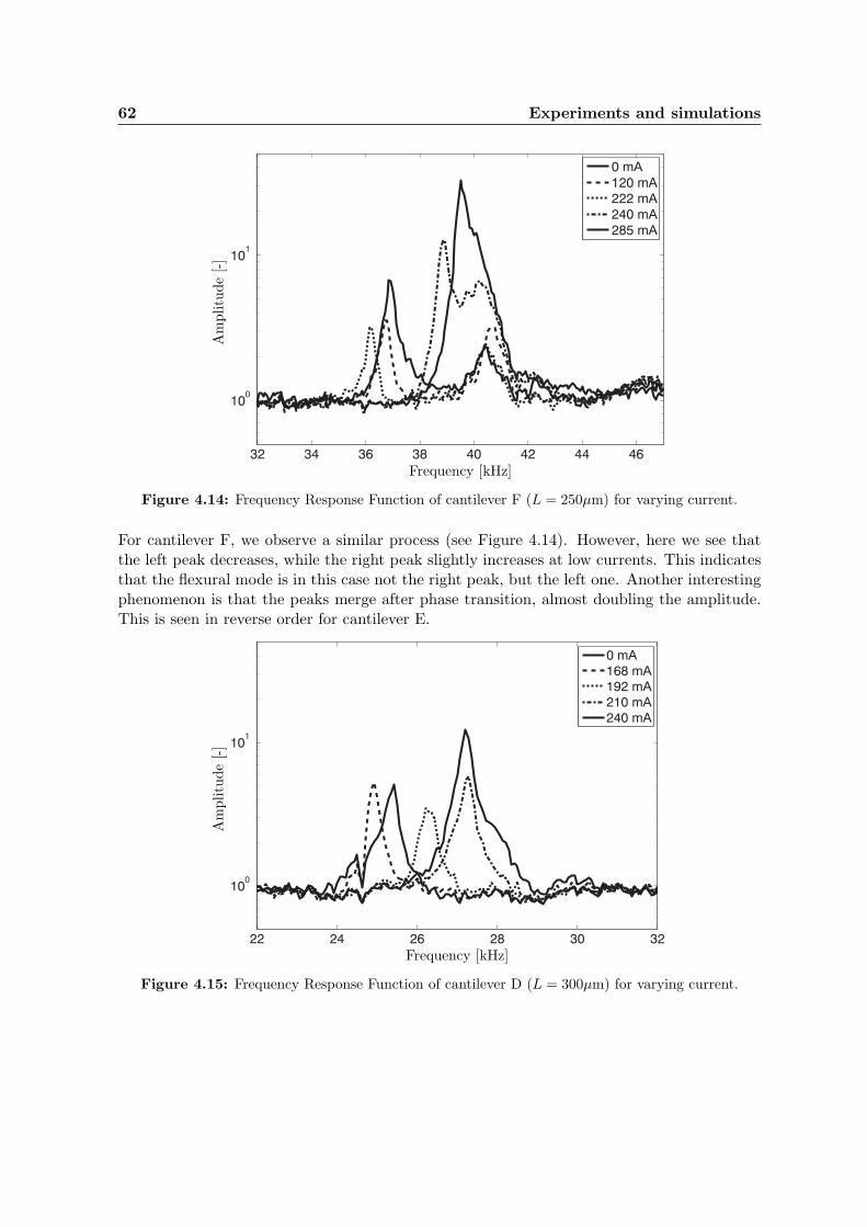
62 Experiments and simulations
32 34 36 38 40 42 44 46
100
101
0 mA
120 mA
222 mA
240 mA
285 mA
Frequency [kHz]
Am
plitu
de
[-]
Figure 4.14: Frequency Response Function of cantilever F (L = 250µm) for varying current.
For cantilever F, we observe a similar process (see Figure 4.14). However, here we see thatthe left peak decreases, while the right peak slightly increases at low currents. This indicatesthat the flexural mode is in this case not the right peak, but the left one. Another interestingphenomenon is that the peaks merge after phase transition, almost doubling the amplitude.This is seen in reverse order for cantilever E.
22 24 26 28 30 32
100
101
0 mA
168 mA
192 mA
210 mA
240 mA
Frequency [kHz]
Am
plitu
de
[-]
Figure 4.15: Frequency Response Function of cantilever D (L = 300µm) for varying current.
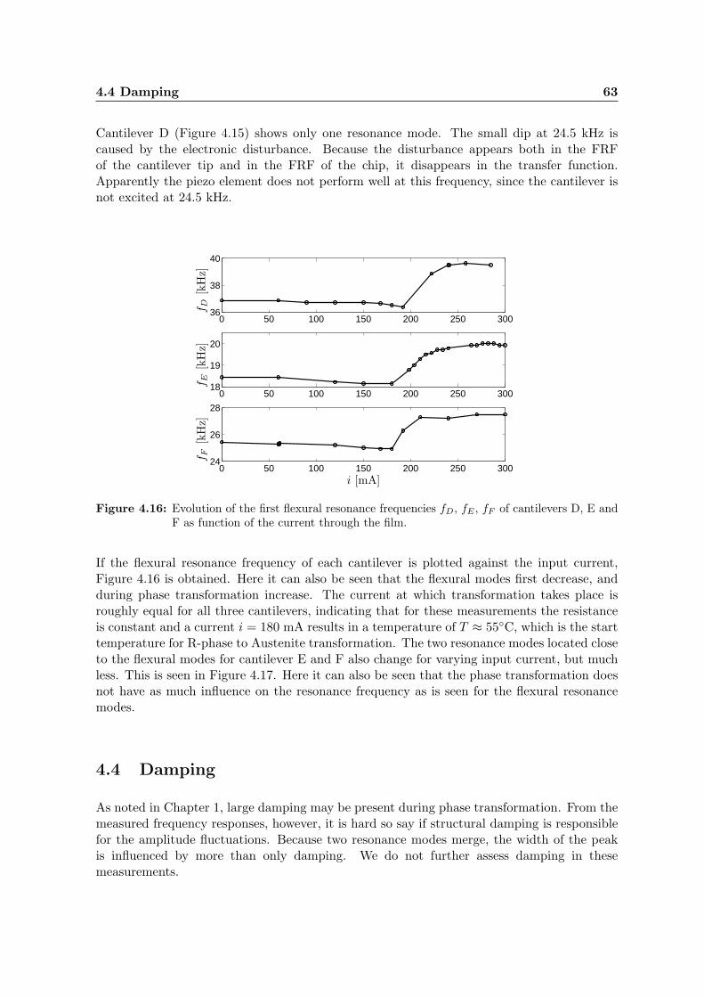
4.4 Damping 63
Cantilever D (Figure 4.15) shows only one resonance mode. The small dip at 24.5 kHz iscaused by the electronic disturbance. Because the disturbance appears both in the FRFof the cantilever tip and in the FRF of the chip, it disappears in the transfer function.Apparently the piezo element does not perform well at this frequency, since the cantilever isnot excited at 24.5 kHz.
0 50 100 150 200 250 30036
38
40
0 50 100 150 200 250 30018
19
20
0 50 100 150 200 250 30024
26
28
f D[k
Hz]
f E[k
Hz]
f F[k
Hz]
i [mA]
Figure 4.16: Evolution of the first flexural resonance frequencies fD, fE , fF of cantilevers D, E andF as function of the current through the film.
If the flexural resonance frequency of each cantilever is plotted against the input current,Figure 4.16 is obtained. Here it can also be seen that the flexural modes first decrease, andduring phase transformation increase. The current at which transformation takes place isroughly equal for all three cantilevers, indicating that for these measurements the resistanceis constant and a current i = 180 mA results in a temperature of T ≈ 55C, which is the starttemperature for R-phase to Austenite transformation. The two resonance modes located closeto the flexural modes for cantilever E and F also change for varying input current, but muchless. This is seen in Figure 4.17. Here it can also be seen that the phase transformation doesnot have as much influence on the resonance frequency as is seen for the flexural resonancemodes.
4.4 Damping
As noted in Chapter 1, large damping may be present during phase transformation. From themeasured frequency responses, however, it is hard so say if structural damping is responsiblefor the amplitude fluctuations. Because two resonance modes merge, the width of the peakis influenced by more than only damping. We do not further assess damping in thesemeasurements.
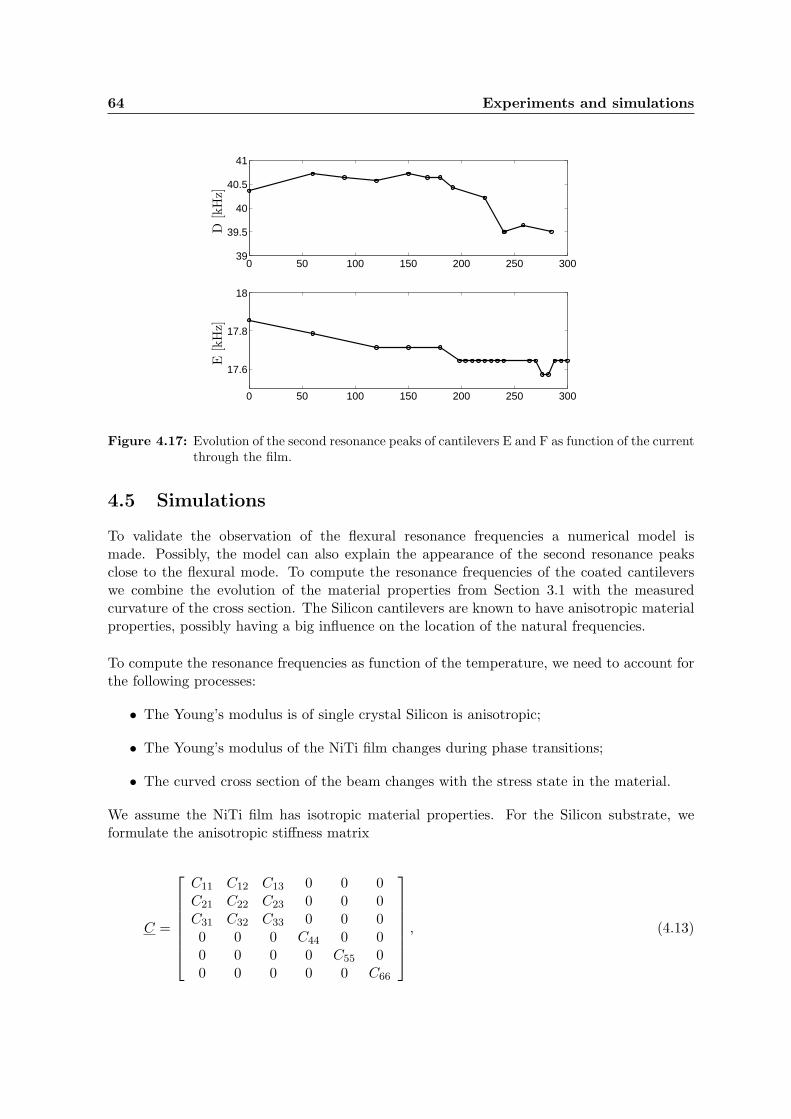
64 Experiments and simulations
0 50 100 150 200 250 30039
39.5
40
40.5
41
0 50 100 150 200 250 300
17.6
17.8
18
D[k
Hz]
E[k
Hz]
Figure 4.17: Evolution of the second resonance peaks of cantilevers E and F as function of the currentthrough the film.
4.5 Simulations
To validate the observation of the flexural resonance frequencies a numerical model ismade. Possibly, the model can also explain the appearance of the second resonance peaksclose to the flexural mode. To compute the resonance frequencies of the coated cantileverswe combine the evolution of the material properties from Section 3.1 with the measuredcurvature of the cross section. The Silicon cantilevers are known to have anisotropic materialproperties, possibly having a big influence on the location of the natural frequencies.
To compute the resonance frequencies as function of the temperature, we need to account forthe following processes:
• The Young’s modulus is of single crystal Silicon is anisotropic;
• The Young’s modulus of the NiTi film changes during phase transitions;
• The curved cross section of the beam changes with the stress state in the material.
We assume the NiTi film has isotropic material properties. For the Silicon substrate, weformulate the anisotropic stiffness matrix
C =
C11 C12 C13 0 0 0C21 C22 C23 0 0 0C31 C32 C33 0 0 00 0 0 C44 0 00 0 0 0 C55 00 0 0 0 0 C66
, (4.13)
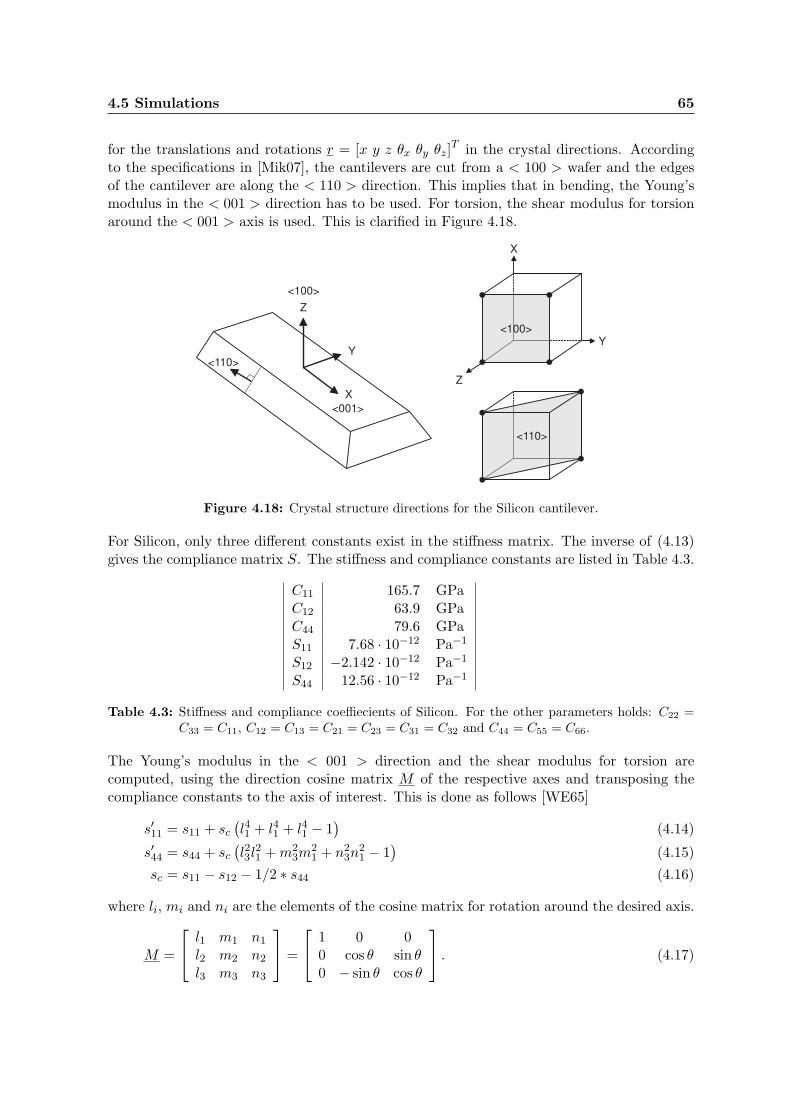
4.5 Simulations 65
for the translations and rotations r = [x y z θx θy θz]T in the crystal directions. According
to the specifications in [Mik07], the cantilevers are cut from a < 100 > wafer and the edgesof the cantilever are along the < 110 > direction. This implies that in bending, the Young’smodulus in the < 001 > direction has to be used. For torsion, the shear modulus for torsionaround the < 001 > axis is used. This is clarified in Figure 4.18.
<100>
<110>
<100>
<110>
<001>
Z
Y
X
X
Z
Y
Figure 4.18: Crystal structure directions for the Silicon cantilever.
For Silicon, only three different constants exist in the stiffness matrix. The inverse of (4.13)gives the compliance matrix S. The stiffness and compliance constants are listed in Table 4.3.
C11 165.7 GPaC12 63.9 GPaC44 79.6 GPaS11 7.68 · 10−12 Pa−1
S12 −2.142 · 10−12 Pa−1
S44 12.56 · 10−12 Pa−1
Table 4.3: Stiffness and compliance coeffiecients of Silicon. For the other parameters holds: C22 =C33 = C11, C12 = C13 = C21 = C23 = C31 = C32 and C44 = C55 = C66.
The Young’s modulus in the < 001 > direction and the shear modulus for torsion arecomputed, using the direction cosine matrix M of the respective axes and transposing thecompliance constants to the axis of interest. This is done as follows [WE65]
s′11 = s11 + sc
(
l41 + l41 + l41 − 1)
(4.14)
s′44 = s44 + sc
(
l23l21 + m2
3m21 + n2
3n21 − 1
)
(4.15)
sc = s11 − s12 − 1/2 ∗ s44 (4.16)
where li, mi and ni are the elements of the cosine matrix for rotation around the desired axis.
M =
l1 m1 n1
l2 m2 n2
l3 m3 n3
=
1 0 00 cos θ sin θ0 − sin θ cos θ
. (4.17)
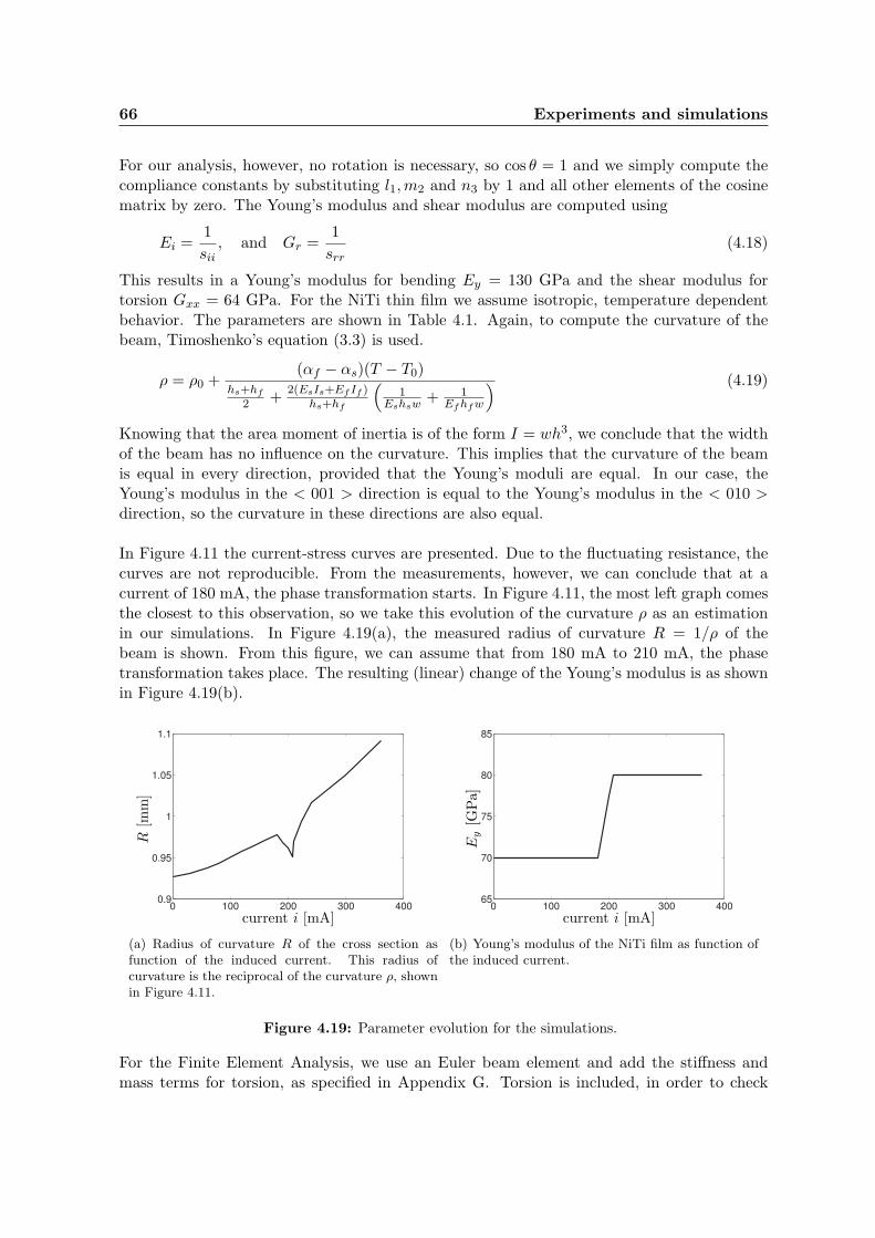
66 Experiments and simulations
For our analysis, however, no rotation is necessary, so cos θ = 1 and we simply compute thecompliance constants by substituting l1, m2 and n3 by 1 and all other elements of the cosinematrix by zero. The Young’s modulus and shear modulus are computed using
Ei =1
sii, and Gr =
1
srr(4.18)
This results in a Young’s modulus for bending Ey = 130 GPa and the shear modulus fortorsion Gxx = 64 GPa. For the NiTi thin film we assume isotropic, temperature dependentbehavior. The parameters are shown in Table 4.1. Again, to compute the curvature of thebeam, Timoshenko’s equation (3.3) is used.
ρ = ρ0 +(αf − αs)(T − T0)
hs+hf
2 +2(EsIs+Ef If )
hs+hf
(
1Eshsw + 1
Ef hf w
) (4.19)
Knowing that the area moment of inertia is of the form I = wh3, we conclude that the widthof the beam has no influence on the curvature. This implies that the curvature of the beamis equal in every direction, provided that the Young’s moduli are equal. In our case, theYoung’s modulus in the < 001 > direction is equal to the Young’s modulus in the < 010 >direction, so the curvature in these directions are also equal.
In Figure 4.11 the current-stress curves are presented. Due to the fluctuating resistance, thecurves are not reproducible. From the measurements, however, we can conclude that at acurrent of 180 mA, the phase transformation starts. In Figure 4.11, the most left graph comesthe closest to this observation, so we take this evolution of the curvature ρ as an estimationin our simulations. In Figure 4.19(a), the measured radius of curvature R = 1/ρ of thebeam is shown. From this figure, we can assume that from 180 mA to 210 mA, the phasetransformation takes place. The resulting (linear) change of the Young’s modulus is as shownin Figure 4.19(b).
0 100 200 300 4000.9
0.95
1
1.05
1.1
current i [mA]
R[m
m]
(a) Radius of curvature R of the cross section asfunction of the induced current. This radius ofcurvature is the reciprocal of the curvature ρ, shownin Figure 4.11.
0 100 200 300 40065
70
75
80
85
current i [mA]
Ey
[GPa]
(b) Young’s modulus of the NiTi film as function ofthe induced current.
Figure 4.19: Parameter evolution for the simulations.
For the Finite Element Analysis, we use an Euler beam element and add the stiffness andmass terms for torsion, as specified in Appendix G. Torsion is included, in order to check
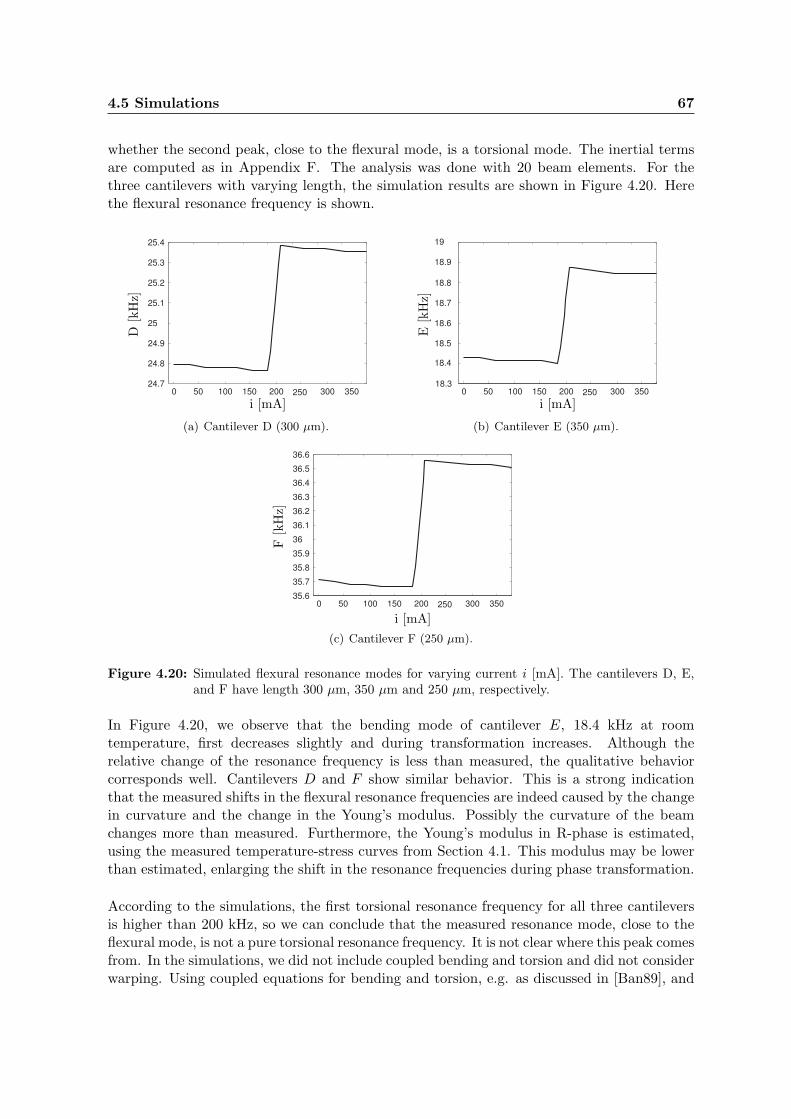
4.5 Simulations 67
whether the second peak, close to the flexural mode, is a torsional mode. The inertial termsare computed as in Appendix F. The analysis was done with 20 beam elements. For thethree cantilevers with varying length, the simulation results are shown in Figure 4.20. Herethe flexural resonance frequency is shown.
24.8
24.9
25
25.1
25.2
25.3
25.4
0 50 100 150 200 250 300 35024.7
D[k
Hz]
i [mA]
(a) Cantilever D (300 µm).
18.4
18.5
18.6
18.7
18.8
18.9
19
0 50 100 150 200 250 300 35018.3
E[k
Hz]
i [mA]
(b) Cantilever E (350 µm).
35.7
35.8
35.9
36
36.1
36.2
36.3
36.4
36.5
0 50 100 150 200 250 300 350
36.6
35.6
F[k
Hz]
i [mA]
(c) Cantilever F (250 µm).
Figure 4.20: Simulated flexural resonance modes for varying current i [mA]. The cantilevers D, E,and F have length 300 µm, 350 µm and 250 µm, respectively.
In Figure 4.20, we observe that the bending mode of cantilever E, 18.4 kHz at roomtemperature, first decreases slightly and during transformation increases. Although therelative change of the resonance frequency is less than measured, the qualitative behaviorcorresponds well. Cantilevers D and F show similar behavior. This is a strong indicationthat the measured shifts in the flexural resonance frequencies are indeed caused by the changein curvature and the change in the Young’s modulus. Possibly the curvature of the beamchanges more than measured. Furthermore, the Young’s modulus in R-phase is estimated,using the measured temperature-stress curves from Section 4.1. This modulus may be lowerthan estimated, enlarging the shift in the resonance frequencies during phase transformation.
According to the simulations, the first torsional resonance frequency for all three cantileversis higher than 200 kHz, so we can conclude that the measured resonance mode, close to theflexural mode, is not a pure torsional resonance frequency. It is not clear where this peak comesfrom. In the simulations, we did not include coupled bending and torsion and did not considerwarping. Using coupled equations for bending and torsion, e.g. as discussed in [Ban89], and
68 Experiments and simulations
including warping may change the location of the resonance frequencies drastically. Especiallywhen the cross section of the cantilever has a large curvature, the influence of warping maybe large. However, it is unlikely that with this analysis the torsional resonance mode of thecantilever shifts with more than a factor 6 down.
Discussion
In this chapter, we have fully characterized and modeled the thermomechanical behavior ofthe NiTi coated cantilever. Thermomechanical measurements provide interesting informationabout the transformation temperatures. The appearance of the R-phase in the workingrange of the current source gives the opportunity to switch between R-phase and Austenitephase during dynamic excitation.
Because the wire contacts on the film are glued, the resistance of the film severely fluctuates.This makes modeling heat transfer by Joule heating problematic. Alternatively, we haveindirectly measured the temperature of the cantilevers during Joule heating and correctedfor the temperature difference between the chip and the freestanding cantilevers.
From the frequency response functions of the cantilevers it can be concluded that thedynamic behavior is significantly influenced by the phase transitions in the material. Thethermal mismatch between the Silicon and NiTi results in a change of curvature of thecross section, subsequently changing the flexural resonance frequency. This change is smallthough, compared to the frequency shift of 10%, caused by the phase transformations.Additionally, these shifts cause separation or merging of the two modes, resulting in adrastic change of their amplitudes. Because of this phenomenon, it is rather difficult tosay anything about damping. If the experiments were conducted with other geometries,e.g. triangular shaped cantilevers, the flexural resonance mode may be more isolatedand it would be less complex to assess the damping behavior of the film. It it not clearwhy two resonance peaks appear close to each other in the measurements. Both peaksshift for varying currents, implying that they are part of the dynamics of the coated cantilever.
Simulations of the flexural resonance frequencies correspond well with the measuredresponses. The small change due to a change of cross section curvature is observed, as well asthe larger frequency shift due to the change of Young’s modulus. The model does not showthe second resonance peak, close to the flexural mode. A dynamical model, capturing moreof the dynamics than only the flexural and torsional modes, could clarify what the origin ofthis resonance peak is.
We conclude that with the SMA coating it is possible to actively influence the dynamics ofthe cantilevers in this setup. Whether this change is significant enough to cancel or dampunwanted vibrations needs to be further investigated. It is interesting to investigate thepossibility to switch between Martensite phase and Austenite phase, instead of the R-phaseand Austenite phase. Because Martensite has a much lower Young’s modulus than Austenite(30 GPa and 80 GPa, respectively), the frequency shifts are larger. Furthermore, investigationof the damping properties is necessary to gain a complete insight in the dynamics and in theapplicability of this design. It can be concluded though, that the coated cantilever gives goodopportunities for vibration control on micro scale and to add functionality in micro devices.
Chapter 5
Conclusions and recommendations
5.1 Conclusions
In this research we have investigated the possibility to actively influence the dynamicalbehavior of micro cantilevers by using a Shape Memory Alloy coating. A equiatomicNickel-Titanium (NiTi) thin film is deposited on commercially available Silicon microcantilevers and consequently annealing the film results in a crystallized NiTi film, showingtemperature- and stress-induced Martensitic transformations. Because NiTi shows largedifferences in its material properties for different phases, the material is useful as a structuralsolution for influencing the dynamics of the cantilever.
Thermomechanics
First the thermomechanical behavior is investigated, using a calibrated heat source andoptical profiler. From temperature-stress curves, the phase transformation temperaturesare determined. The hysteresis curve is large, because the phase transformations are bothtemperature- and stress-induced. Because the stress levels in the material are low, a two-steptransformation takes place when cooling from Austenite phase. This is the R-phase, whichappears at 58.5 C.
Experimental setup
An experimental setup is designed, suitable for investigating the dynamic response of microcantilevers to an excitation, while the temperature of the NiTi film can be varied by anelectrical current. The setup is capable of measuring small displacements (< 100 nm) athigh frequency (up to 100 kHz). In the frequency domain, accurate frequency responsemeasurements are possible.
Modeling
To understand and predict the behavior of the coated cantilevers, a thermomechanical modelis made. This model gives insights in the transformation behavior of the material. Thebimorph effect due to a mismatch in thermal expansion is modeled using Timoshenko’sequation for bimetallic thermostats, extended to include temperature dependent stiffness. Fordescribing the hysteretic transformation behavior several mathematical models of hysteresis
70 Conclusions and recommendations
are proposed. To fit the measurements the Krasnosel’skii-Pokrovskii hysteron is used,because it has an appealing simplicity, while still capable of modeling the complex hysteresisloops. Minor loops are represented by horizontal lines, but still the model represents thephase transformation behavior of the material well.
A 1D heat transfer model is formulated, describing the conduction, convection and Jouleheating of the NiTi film. For estimating the electrothermal interaction, the temperaturedependent resistivity is required. This is hard to measure, because the electrical circuitexperiences resistance fluctuations due to the quality of the glued contacts. Because thetemperature of the cantilever cannot be measured directly, validation of the model is notpossible. Alternatively the thermal response is measured indirectly by measuring the profileof the cantilever for a controlled temperature and comparing this to the thermomechanicalresponse on the electrical current. Because the resistance fluctuates, it still is difficult todetermine the exact temperature of the cantilevers.
Experiments
The measured frequency response functions of the cantilevers show that changing thetemperature of the film significantly influences the dynamics of the cantilevers. Themeasurements show two resonance peaks close to each other, of which one is identified as theflexural resonance mode. The appearance of the second resonance peak in not clear. Due toa change in the profile of the cross section, the flexural stiffness decreases for an increasingcurrent. Phase transition from R-phase to Austenite phase increases the Young’s modulus,resulting in an increase of the flexural resonance frequency of as much as 10%. The secondmode only change slightly. The two resonance peaks merge and separate under varying inputcurrents, resulting in a change of amplitude. Because of this observation it is difficult toassess damping of the system.
The resonance frequencies of the beam are computed, using standard formulations of flexuraland torsional stiffness and a finite element analysis. In these simulations the changing areamoment of inertia and Young’s modulus are taken into account. The simulations showthat the flexural resonance mode indeed is influenced by the changing cross section of thecantilever and by the change in the Young’s modulus. The frequency shifts are smaller thanthe measured ones, probably because the cross section curvature changes more than assumedand because the Young’s modulus in the R-phase is not estimated correctly. The simulationsalso show that the second peak, close to the flexural resonance mode, is not likely to be atorsional resonance frequency.
We can conclude that a NiTi coating on these cantilevers significantly influence its dynamicresponse. The amount of damping that the NiTi film adds is difficult to determine, becausethe modes are close to each other.
5.2 Recommendations 71
5.2 Recommendations
For future work on this topic, recommendations are done in both the experimental and in theanalytical part of the research. We also discuss future work.
Experiments
For more accurate experiments, the setup for dynamic experiments can be improved.Although the LDGU is suitable for qualitatively measuring small displacements at a highfrequency, its performance depends greatly on the reflectivity of the sample and howwell it is aligned. Furthermore, the focusing lens has to be within 3mm of the sample,making access to the sample and shielding from the electromagnetic radiation of the piezoelement problematic. A measurement principle for larger distance, for example a calibratedlaser-diode combination as used in Atomic Force Microscopes, would greatly improve theflexibility of the setup.
Sample preparation was a very elaborate task in this project. Sputtering and annealingof the thin film on the cantilever chip was done very well, but attaching wires to the chipdid not give satisfactory electrical properties. Sputter coating the chip partially with goldor silver can solve these problems, because then ultrasonic wirebonding will have morechance of giving good bonds. Moreover, a reproducible and accurate measurement of thefilm resistance as function of the induced current is useful for understanding both theelectrothermal properties of the film and the phase transformation behavior. A four-pointresistivity measurement is desired and could give good results, provided the wirebonds are ofgood quality. Because the resistance of the film is fluctuating severely, an accurate estimationof the cantilever temperature for varying current is not possible. It is recommended toinvestigate possibilities to directly measure the cantilever temperature. If the film is wellconnected to a current source, an indirect measurements could also give satisfactory results.
It is recommended to repeat the experiments with coated cantilevers with other dimensionsand geometries. This may make interpretation of the frequency response functions lesscomplex, because separate resonance peaks can be analyzed. It may also give the opportunityto investigate the damping properties of the material, which in our case is problematic.
Modeling
For modeling hysteresis in the phase transformations, several modeling approaches arepresented. These are only a few options for mathematical modeling of hysteresis. A thoroughinvestigation on other available models, as well as improvement of the proposed models canlead to a more accurate approximation of the hysteresis curves. Furthermore, a physicalmodel describing the kinematics of transformation can improve the understanding of thethermomechanical behavior of the NiTi coated cantilever.
The measured frequency response functions only partially explain the dynamic behavior of thecoated cantilevers. It is recommended to investigate the dynamical behavior of the coatedcantilevers in more detail. If the model is extended to describe more than flexural andtorsional modes, we may be able to better understand the measured dynamical behavior ofthe cantilevers.
72 Conclusions and recommendations
Future work
In this research we have made choices for the dimensions of the cantilevers, the thickness ofthe deposited SMA film and the way of heating the film. These decisions have determinedthe frequency range of interest, the temperature range of interest and the thermomechanicalcharacteristics of the samples. Concerning the range of applications of the cantileversas a sensor or actuator, other geometries may be more favorable. A study on specificapplications for coated cantilevers will provide requirements for the cantilever dimensionsand may help in choosing the right film composition and thickness. The transformationtemperatures can vary severely for varying film composition and film thickness, so it isimportant to select the right material for the right application. These choices are ofgreat influence on the effect of the phase transformation on the dynamics of the cantileverand thus determine the succes of this solution for structural vibration control of micro systems.
Shape Memory Alloys have several extraordinary properties. In this research we haveinvestigated the influence of a change in the material properties on the dynamics of a microcantilever. We did not consider the Shape Memory Effect or Superelasticity Effect. Thesetwo phenomena - also a result of phase transformations - are very interesting to use foractuating a (micro) device. Numerous publications (e.g. [KLR+96] and [DGD05]) report theuse of these mechanisms in micro and macro applications. It is recommended to investigatewhether a combination of our research with existing knowledge about SMA materials givesmore opportunities for using it to add functionality and efficiency in the design of sensors andactuators.
Bibliography
[Ban89] J.R. Banerjee, Coupled bending-torsional dynamic stiffness matrix for beamelements, International journal for numererical methods in engineering 28 (1989),1283–1298.
[BB98] A Bekker and L.C. Brinson, Phase diagram based description of the hysteresisbehavior of shape memory alloys, Acta Materialia 46 (1998), no. 10, 3649–3665.
[BL96] J.G. Boyd and D.C. Lagoudas, A thermodynamical constitutive model for shapememory materials. part i. the monolithic shape memory alloy, Internation Journalof Plasticity 12 (1996), no. 6, 805–842.
[DG05] S.M. Dutta and F.H. Ghorbel, Differential hysteresis modeling of a shape memoryalloy wire actuator, IEEE/ASME Transactions of Mechatronics 10 (2005), no. 2,189–197.
[DGD05] S.M. Dutta, F.H. Ghorbel, and J.B. Dabney, Modeling and control of a shapememory alloy actuator, Proceedings of the 2005 IEEE International Symposiumon Intelligent Control, Limassol, Cyprus (2005).
[HW97] D. Hughes and J.T. Wen, Preisach modeling of piezoceramic and shape memoryalloy hysteresis, Smart Material Structures 6 (1997), 287–300.
[ITH91] K. Ikuta, T Tsukamoto, and S Hirose, Mathematical model and experiemntalverification of shape memory alloy for designing micro actuator, IEEE Proceedingsof the MEMS’91 (1991), 103–108.
[Jan00] W.S. Janna, Engineering heat transfer, second edition ed., CRC Press LLC, BocaRaton, Florida, USA, 2000.
[KLR+96] P. Krulevitch, A.P. Lee, P.B. Ramsey, J.C. Trevino, J. Hamilton, andM.A. Northrup, Thin film shape memory alloy microactuators, Journal ofMicroelectromechanical Systems 5 (1996), no. 4, 270–282.
[KP89] M.A. Krasnosel’skii and A.V. Pokrovskii, Systems with hysteresis, Springer Verlag,Berlin, Germany, 1989.
[May91] I.D. Mayergoyz, Mathematical models of hysteresis, Springer Verlag, New York,USA, 1991.
[McG07] McGill University, Canada, http://www.mcgill.ca, consulted September 2007.
74 BIBLIOGRAPHY
[MEM07] MEMX, http://www.memx.com, consulted September 2007.
[Mic08] Microfabrication Laboratory at Northeastern University, http://www.ece.neu.edu,consulted June 2008.
[Mik07] MikroMasch, http://www.spmtips.com, consulted April 2007.
[MNZ93] J.W. Macki, P. Nistri, and P. Zecca, Mathematical models for hysteresis, SIAMReview 35 (1993), no. 1, 94–123.
[NYU07] NYU School of Medicine, Microbiology, http://biosingularity.wordpress.com,Biosingularity, consulted September 2007.
[OB05] J. Oh and D.S. Bernstein, Semilinear duhem model for rate-independent andrate-dependent hysteresis, IEEE Transactions on Automatic Control 50 (2005),no. 5, 631–645.
[OR05] K. Otsuka and X. Ren, Physical metallurgy of tini-based shape memory alloys,Progress in Materials Science 50 (2005), 511–678.
[Phi00] Philips Optical Storage, Vam1202/12 cd mechanism for 2x speed, data sheet,September 2000.
[Phi01] Phisik Instrumente, Product Catalogue, Micropositioning, nanopositioning,nanoautomation. solutions for curring edge technologies, 2001.
[Pre35] F. Preisach, Uber die magnetische nachwirkung, Zeitschrift fur Physik 94 (1935),277–302.
[Pri02] W.O Pril, Development of high precision mechanical probes for coordinatemeasuring machines, Ph.D. thesis, Technische Universiteit Eindhoven, 2002.
[San08] Sandia National Laboratories, http://mems.sandia.gov, consulted June 2008.
[Sch04] W. Schwanen, Modeling and identification of the dynamic behavior of a wirerope spring, Master’s thesis, Eindhoven University of Technology, Eindhoven,Netherlands, 2004.
[Sou07] Southwest Research Institute, http://www.swri.org, consulted April 2007.
[Tim25] S. Timoshenko, Analysis of bi-metallic thermostats, Journal of the Optical Societyof America 11 (1925), 233–255.
[VDI02] VDI-Warmeatlas, vol. 9, Springer, Berlin, 2002.
[Vel05] W.P. Vellinga, Lecture notes on the course microscopic measurement techniques,2005.
[Vis94] A. Visintin, Differential models of hysteresis, Springer, Berlin, Germany, 1994.
[VZ65] E Volterra and E.C. Zachmanoglou, Dynamics of vibrations, Charles E. MerrillBooks, Columbus, Ohio, USA, 1965.
BIBLIOGRAPHY 75
[Wan07] X. Wang, Chrystallization and martensitic transformation behavior of nitishape memory alloy thin films, Ph.D. thesis, Harvard University, Cambridge,Massachusetts, USA, 2007.
[WE65] J.J. Wortman and R.A. Evans, Young’s modulus, shear modulus, and poisson’sratio in silicon and germanium, Journal of Applied Physics 36 (1965), no. 1,153–156.
[Wij98] M. van der Wijst, Shape control of structures and materials with shape memoryalloys, Phd thesis, Eindhoven University of Technology, Eindhoven, Netherlands,1998.
[Wut03] M. Wuttig, High damping of inhomogeneous ferroics, Journal of Alloys andCompounds 355 (2003), 108–112.
[You89] W.C. Young, Roark’s formulas for stress and strain, sixth edition, McGraw-Hill,USA, 1989.

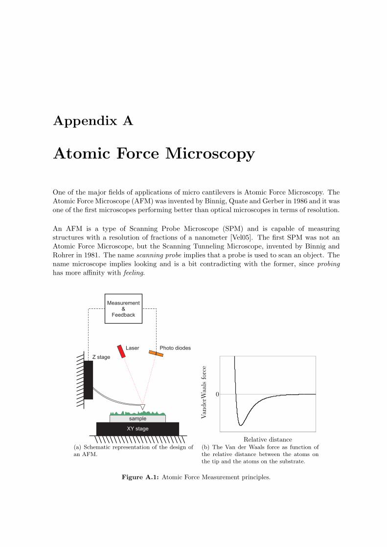
Appendix A
Atomic Force Microscopy
One of the major fields of applications of micro cantilevers is Atomic Force Microscopy. TheAtomic Force Microscope (AFM) was invented by Binnig, Quate and Gerber in 1986 and it wasone of the first microscopes performing better than optical microscopes in terms of resolution.
An AFM is a type of Scanning Probe Microscope (SPM) and is capable of measuringstructures with a resolution of fractions of a nanometer [Vel05]. The first SPM was not anAtomic Force Microscope, but the Scanning Tunneling Microscope, invented by Binnig andRohrer in 1981. The name scanning probe implies that a probe is used to scan an object. Thename microscope implies looking and is a bit contradicting with the former, since probinghas more affinity with feeling.
(a) Schematic representation of the design ofan AFM.
0
Relative distance
Van
der
Waa
lsfo
rce
(b) The Van der Waals force as function ofthe relative distance between the atoms onthe tip and the atoms on the substrate.
Figure A.1: Atomic Force Measurement principles.
78 Atomic Force Microscopy
In Figure A.1(a) the schematic layout of a certain type of AFM is shown. A micro cantileverwith a very sharp tip - at the end only several atoms wide - is brought close to the surfaceof the substrate, in the order of a few nanometers. The interaction between the substratesurface and the cantilever tip results in deflection of the tip. One of the important forces inthis range is the Van der Waals force, shown in Figure A.1(b). When the tip is relativelyfar away from the surface, the forces are small and the tip does not feel the surface.Coming closer, the tip is firstly attracted to the surface due to the attractive Van der Waalsforce. When brought closer, this force will become repulsive. Other interacting forces aremechanical contact forces, capillary forces, chemical bonding, electrostatic and magneticforces. Analysis of these forces gives opportunities to investigate several properties of thesubstrate.
The cantilever is connected to a Z-stage, consisting of a piezo element. The stage has aresolution in the range of 0.1 nm (1 A). The substrate is placed on an XY-stage, that movesthe sample under the tip. This way, the tip probes the surface area of the sample. The tipwill encounter a change in topography when the XY-stage is scanning it. This will bringthe tip closer or further to the surface and consequently the interacting forces result indeflection of the cantilever. This deflection is measured by a laser-diode combination andfed back to the Z-stage, which will correct for the position change. The effort, needed tobring the tip back to its original position, gives information about the surface topographyand other mechanical or physical properties. If the cantilever is charged or heated, electricaland thermal properties can be investigated.
Disturbing vibrations of the cantilever introduce measurement errors and noise. Thesedisturbances can come from the surroundings or from moving parts in the AFM. The setupis therefore isolated from the surroundings as good as possible and sophisticated designprinciples and control algorithms for the piezo stages are used.
Appendix B
PIC181 PZT material properties
The specifications of the used piezo ceramic material are shown in Figure B.1. The piezoelements are fabricated by Physik Instrumente (PI) and distributed by Applied LaserTechnologies in Best, the Netherlands. At PI, two types of piezo ceramics are available:’soft’and ’hard’ ceramics. ’Soft’ refers to piezo’s which require less power to expand, buthave a low quality factor (high damping), so dissipate more energy. ’Hard’ piezo’s need morepower, but dissipate less energy, are very stiff and have a high quality factor. They aresuitable for high power applications and oscillators [Phi01]. PIC181 is a hard ceramic withan extremely high quality factor and a high curie temperature, making it suitable for highfrequency applications.
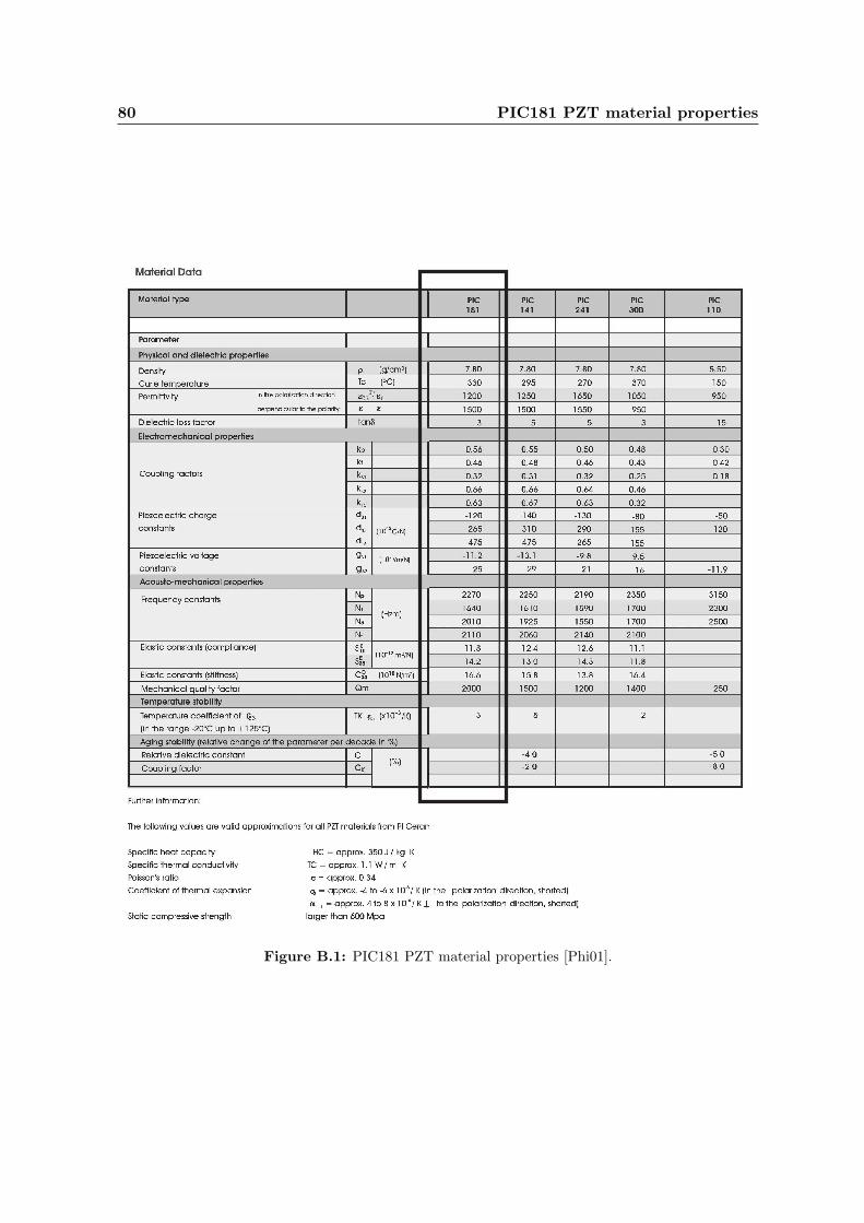
80 PIC181 PZT material properties
Figure B.1: PIC181 PZT material properties [Phi01].
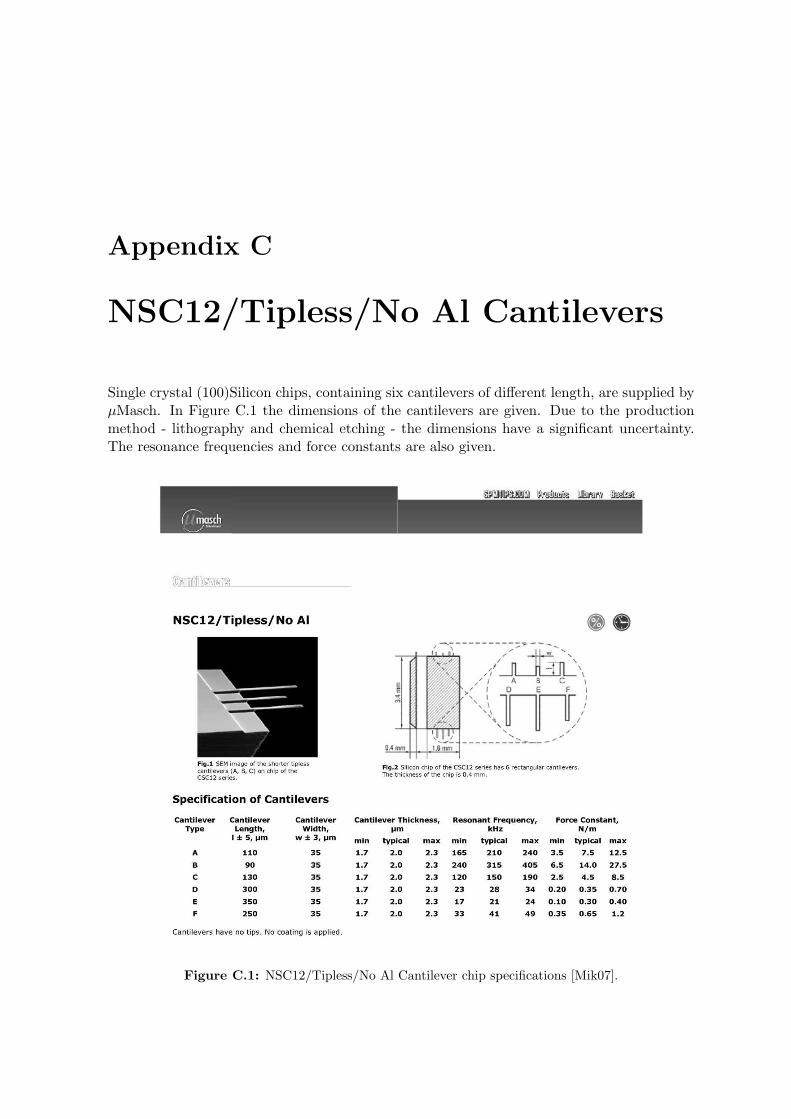
Appendix C
NSC12/Tipless/No Al Cantilevers
Single crystal (100)Silicon chips, containing six cantilevers of different length, are supplied byµMasch. In Figure C.1 the dimensions of the cantilevers are given. Due to the productionmethod - lithography and chemical etching - the dimensions have a significant uncertainty.The resonance frequencies and force constants are also given.
Figure C.1: NSC12/Tipless/No Al Cantilever chip specifications [Mik07].

Appendix D
Piezo amplifier design
The electrical design of the piezo amplifier is shown in Figure D.1. The layout was designedby Michael Hopper. The Central Technical Services (GTD) of the Eindhoven University ofTechnology have made some adjustments and have built the amplifier with additional coolingfacilities. It uses a 400 V, 600 mA power supply and the input is generated using NI Labviewand a 1.25 MHz NI-USB 6251 data acquisition card.
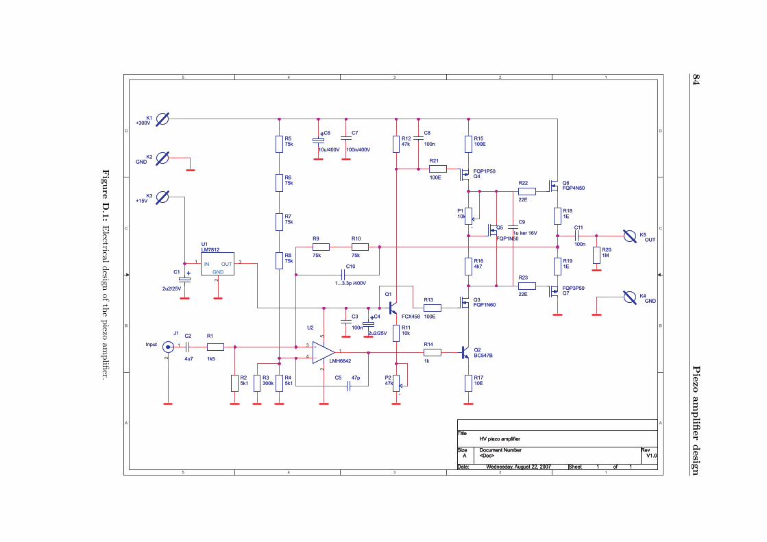
84
Pie
zo
am
plifi
er
desig
n5
5
4
4
3
3
2
2
1
1
D D
C C
B B
A A
Title
Size Document Number Rev
Date: Sheet of
<Doc> V1.0
HV piezo amplifier
A
1 1Wednesday, August 22, 2007
Title
Size Document Number Rev
Date: Sheet of
<Doc> V1.0
HV piezo amplifier
A
1 1Wednesday, August 22, 2007
Title
Size Document Number Rev
Date: Sheet of
<Doc> V1.0
HV piezo amplifier
A
1 1Wednesday, August 22, 2007
C3
100n
C3
100n
+
P247k
+
P247k
C10
1...3.3p /400V
C10
1...3.3p /400V
C7
100n/400V
C7
100n/400V
Q4FQP1P50Q4FQP1P50
R1
1k5
R1
1k5
C8
100n
C8
100nR575kR575k
R875kR875k
R1110kR1110k
Q2BC547BQ2BC547B
R191ER191E
R25k1R25k1
R45k1R45k1
Q7FQP3P50Q7FQP3P50
K4GND
K4GND
U1LM7812U1LM7812
IN1 OUT 3
2
GND
C11
100n
C11
100n
K5OUT
K5OUT
C9
1u ker 16V
C9
1u ker 16V
K1+300V
K1+300V
R1710ER1710E
R10
75k
R10
75k
-
+
U2
LMH6642-
+
U2
LMH6642
3
41
52
C5 47pC5 47p
C2
4u7
C2
4u7
+C1
2u2/25V
+C1
2u2/25V
R201MR201M
R15100ER15100E
+
P110k
+
P110k
R181ER181E
R22
22E
R22
22E
R775kR775k
R9
75k
R9
75k
R3300kR3300k
K2GND
K2GND
Q6FQP4N50Q6FQP4N50
Q1
FCX458
Q1
FCX458
R1247kR1247k
+C4
2u2/25V
+C4
2u2/25V
Q3FQP1N60Q3FQP1N60
K3+15V
K3+15V
+C6
10u/400V
+C6
10u/400V
R21
100E
R21
100E
Q5
FQP1N50
Q5
FQP1N50
R675kR675k
R13
100E
R13
100E
R164k7R164k7
J1
Input
J1
Input 1
2
R23
22E
R23
22E
R14
1k
R14
1k
Fig
ure
D.1
:E
lectricaldesign
ofth
epiezo
amplifi
er.
Appendix E
LDGU amplifier design
The electrical design of the LDGU amplifier is shown in Figure E.1. The Central TechnicalServices (GTD) of the Eindhoven University of Technology has designed and built theamplifier, according to specifications in [Phi00].
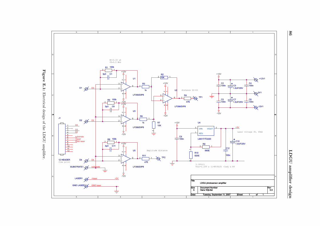
86
LD
GU
am
plifi
er
desig
n5
5
4
4
3
3
2
2
1
1
D D
C C
B B
A A
+3V
D2
D4
+3V+laser
D3
substrate
D4
D2
substrate+laserGND laser
GND laser
D3
+12V
+12V+12V
+12V
+12V
+12V
-12V
-12V
-12V
-12V
-12V
Title
Size Document Number Rev
Date: Sheet of
Hans Wijtvliet 0.0
LDGU photosensor amplifier
A
1 1Tuesday, September 11, 2007
Title
Size Document Number Rev
Date: Sheet of
Hans Wijtvliet 0.0
LDGU photosensor amplifier
A
1 1Tuesday, September 11, 2007
Title
Size Document Number Rev
Date: Sheet of
Hans Wijtvliet 0.0
LDGU photosensor amplifier
A
1 1Tuesday, September 11, 2007
Laser voltage 3V, 40mA
distance D2-D3
Amplitude distance
flex print
RC=0.33 uSf0=0.5 Mhz
3.16VoltVout=1.25V x (1+R9/R10) +Iadj x R9
R8 100kR8 100k
12
C9100nC9100n
TP1TP1C6100nC6100n
R4
47E
R4
47E
12
-
+
U2
LF356/DIP8
-
+
U2
LF356/DIP8
3
26
7 14 5
+C7
1.0UF/25V
+C7
1.0UF/25V
TP2TP2R11
47E
R11
47E
12
+12V1+12V1
R3
1k
R3
1k
12D1D1
C13p3 C13p3
U4
LM317/TO220
U4
LM317/TO220
VIN3
ADJ1
VOUT 2
0V10V1
-
+
U5
LF356/DIP8
-
+
U5
LF356/DIP8
3
26
7 14 5
J1
12 HEADER
J1
12 HEADER
123456789101112
D2D2
R2
10K
R2
10K 12
C83p3 C83p3 -12V1-12V1
C5100nC5100n
-
+
U1
LF356/DIP8
-
+
U1
LF356/DIP8
3
26
7 14 5
D4D4
R9
560E
R9
560E
12
R6
1k
R6
1k
12
R1 100kR1 100k
12
+C10
1.0UF/25V
+C10
1.0UF/25V
SUBSTRATE1SUBSTRATE1
C113p3 C113p3
C2100nC2100n
LASER1LASER1
R7
10K
R7
10K
12
-
+
U3
LF356/DIP8
-
+
U3
LF356/DIP8
3
26
7 14 5
R5 100kR5 100k
12
C12
100n
C12
100nR10
820E
R10
820E
12
C4100nC4100n
GND LASER1GND LASER1
+C3
1.0UF/25V
+C3
1.0UF/25V
Fig
ure
E.1
:E
lectricaldesign
ofth
eLD
GU
amplifi
er.
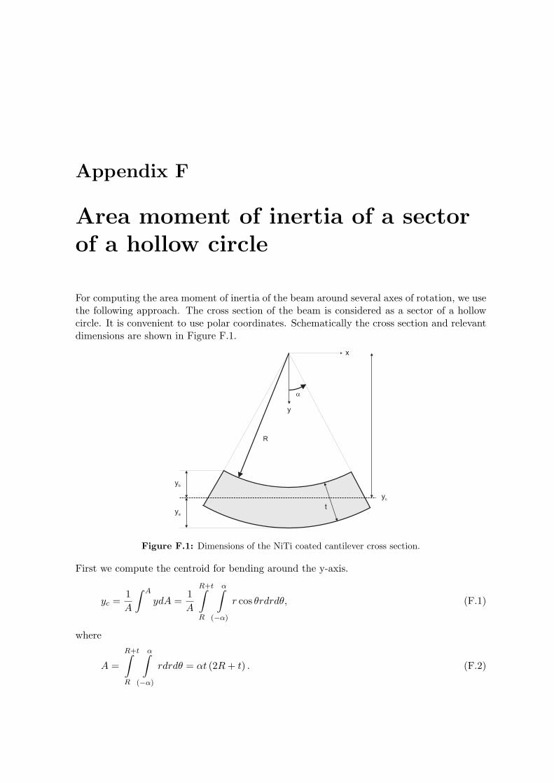
Appendix F
Area moment of inertia of a sectorof a hollow circle
For computing the area moment of inertia of the beam around several axes of rotation, we usethe following approach. The cross section of the beam is considered as a sector of a hollowcircle. It is convenient to use polar coordinates. Schematically the cross section and relevantdimensions are shown in Figure F.1.
R
a
x
y
ya
yb
yc
t
Figure F.1: Dimensions of the NiTi coated cantilever cross section.
First we compute the centroid for bending around the y-axis.
yc =1
A
∫ A
ydA =1
A
R+t∫
R
α∫
(−α)
r cos θrdrdθ, (F.1)
where
A =
R+t∫
R
α∫
(−α)
rdrdθ = αt (2R + t) . (F.2)
88 Area moment of inertia of a sector of a hollow circle
This gives
yc =2 sin α
3α
(
3R2 + 3Rt + t2)
(2R + t)=
2 sinα
3α
(
R + t +R2
2R + t
)
. (F.3)
The inertia around the x-axis is computed through
Iy0 =
∫ A
y2dA =
R+t∫
R
α∫
(−α)
r2 cos2 θrdrdθ, (F.4)
Steiner’s law gives the inertia around the centroid yc
Iy = Iy0 − y2cA (F.5)
=1
4t(2R + t)(2R2 + 2Rt + t2)(cos α sinα + α) − 4 sin2 α
9α
(3R2 + 3Rt + t2)2t
(2R + t). (F.6)
Similarly, for the moment of inertia around the z-axis we write
Iz =1
4t(2R + t)(2R2 + 2Rt + t2)(− cos α sinα + α). (F.7)
For both the film and the cantilever, the inertia with respect to their own centroid is computed,simply by integrating over R+hf and R for the film and over R+hf +hs and R+hf for thecantilever. The centroid of the total cross section is computed by integrating over R+hf +hs
and R. The inertia of the elements with respect to this centroid can be computed usingSteiner’s law.
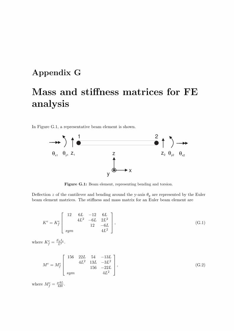
Appendix G
Mass and stiffness matrices for FEanalysis
In Figure G.1, a representative beam element is shown.
z1θy1θx1z2 θy2 θx2z
xy
1 2
Figure G.1: Beam element, representing bending and torsion.
Deflection z of the cantilever and bending around the y-axis θy are represented by the Eulerbeam element matrices. The stiffness and mass matrix for an Euler beam element are
Ke = Kef
12 6L −12 6L4L2 −6L 2L2
12 −6Lsym 4L2
, (G.1)
where Kef =
EyIy
L3 .
M e = M ef
156 22L 54 −13L4L2 13L −3L2
156 −22Lsym 4L2
, (G.2)
where M ef = ρAL
420 .
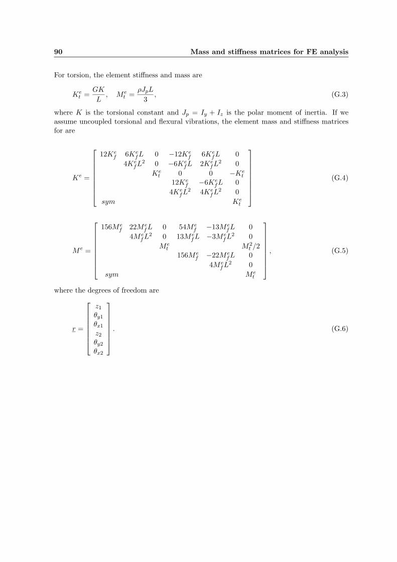
90 Mass and stiffness matrices for FE analysis
For torsion, the element stiffness and mass are
Ket =
GK
L, M e
t =ρJpL
3, (G.3)
where K is the torsional constant and Jp = Iy + Iz is the polar moment of inertia. If weassume uncoupled torsional and flexural vibrations, the element mass and stiffness matricesfor are
Ke =
12Kef 6Ke
fL 0 −12Kef 6Ke
fL 0
4KefL2 0 −6Ke
fL 2KefL2 0
Ket 0 0 −Ke
t
12Kef −6Ke
fL 0
4KefL2 4Ke
fL2 0
sym Ket
(G.4)
M e =
156M ef 22M e
fL 0 54M ef −13M e
fL 0
4M efL2 0 13M e
fL −3M efL2 0
M et M2
t /2156M e
f −22M efL 0
4M efL2 0
sym M et
, (G.5)
where the degrees of freedom are
r =
z1
θy1
θx1
z2
θy2
θx2
. (G.6)
Appendix H
Dynamic measurements
The dynamic measurements were conducted on the three coated cantilevers with theapproximate length of 250 µm (Figure H.1), 300 µm (Figure H.2) and 350 µm (Figure H.3).The cantilevers and chip are excited by a white noise signal with an amplitude of 0.05 V,amplified to ∼5 V by the piezo amplifier. The diode signal D2 − D3 is acquired by the NIUSB-6251 at a rate of 700 kHz, with 10.000 samples per measurement interval. The Nyquistfrequency - the highest reconstructible frequency - thus is 350 kHz. The frequency resolutionis
fr =fm
N= 70 Hz, (H.1)
where fm is the sample rate and N is the number of samples per measurement interval.The measurement time interval is 14.3 ms. The shown responses are an average over 200measurements and a Hanning window is used to reduce signal leaking.
To properly visualize the difference between the responses, they are given a certain offset. Thisgives a clear sight on the evolution of both the location and the amplitude of the resonancefrequencies in the relevant frequency range.

92 Dynamic measurements
Frequency [kHz]
Am
plitu
de
[arb
.u.]
Curr
ent
[mA
]
0
63
86
110
122
151
169
181
192
210
240
269
299
22 25 26 28 30 32
Figure H.1: Frequency response functions of cantilever D, with length L = 300µm.
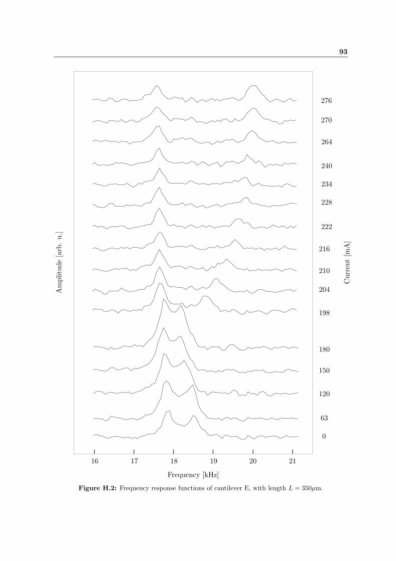
93
Frequency [kHz]
Am
plitu
de
[arb
.u.]
Curr
ent
[mA
]
0
63
120
150
180
198
204
210
216
222
228
234
240
264
270
276
16 17 18 19 20 21
Figure H.2: Frequency response functions of cantilever E, with length L = 350µm.
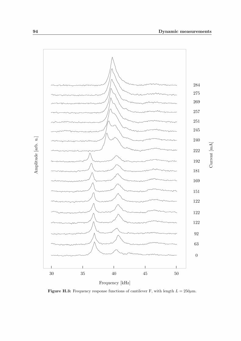
94 Dynamic measurements
Frequency [kHz]
Am
plitu
de
[arb
.u.]
Curr
ent
[mA
]
0
63
92
122
122
122
151
169
181
192
222
240
245
251
257
269
275
284
30 35 40 45 50
Figure H.3: Frequency response functions of cantilever F, with length L = 250µm.