dynamics and control of flexible multibody … · dynamics and control of flexible multibody...
TRANSCRIPT
DYNAMICS AND CONTROL
OF
FLEXIBLE MULTIBODY STRUCTURES
Timothy J. Stemple
Dissertation submitted to the faculty of the Virginia Polytechnic Instituteand State University in partial fullfillment of the requirement for the degree of
Doctor of Philosophyin
Engineering Science and Mechanics
Leonard Meirovitch, ChairmanWilliam T. Baumann
Scott L. HendricksRobert C. RogersMark S. Cramer
March 19, 1998Blacksburg, Virginia
Keywords: multibody dynamics, flexible multibody structures, control
cCopyright ©1998, by Timothy J. Stemple
DYNAMICS AND CONTROL OF FLEXIBLE MULTIBODY STRUCTURES
Timothy J. Stemple
(ASTRACT)
The goal of this study is to present a method for deriving equations of motion capable ofmodeling the controlled motion of an open loop multibody structure comprised of an arbi-trary number of rigid bodies and slender beams. The procedure presented here for derivingequations of motion for flexible multibody systems is carried out by means of the Principleof Virtual Work (often referred to in the dynamics literature as d’Alembert’s Principle).
We first consider the motion of a general flexible body relative to the inertial space, andthen derive specific formulas for both rigid bodies and slender beams. Next, we make a smallmotions assumption, with the end result being equations for a Rayleigh beam, which includeterms which account for the axial motion, due to bending, of points on the beam central axis.This process includes a novel application of the exponential form of an orthogonal matrix,which is ideally suited for truncation. Then, the generalized coordinates and quasi-velocitiesused in the mathematical model, including those needed in the spatial discretization processof the beam equations are discussed. Furthermore, we develop a new set of recursive relationsused to compute the inertial motion of a body in terms of the generalized coordinates andquasi-velocities.
This research was motivated by the desire to model the controlled motion of a flexiblespace robot, and consequently, we use the multibody dynamics equations to simulate themotion of such a structure, providing a demonstration of the computer program. For thisparticular example we make use of a new sequence of shape functions, first used by Meirovitchand Stemple to model a two dimensional building frame subjected to earthquake excitations.

for Monica
ACKNOWLEDGEMENT
First and foremost I would like to thank my advisor, Professor Leonard Meirovitch, for hiscontinued support and guidance of both my research and career.
I also want to express my gratitude to committee members Drs. William T. Baumann,Scott L. Hendricks, Robert C. Rogers and Mark S. Cramer, for reviewing my dissertation,and for the part they played in furthering my education.
And finally, I am grateful to Professor Edmund G. Henneke and the ESM departmentfor affording me the opportunity to study and teach at Virginia Tech.
Contents
1 Introduction 11.1 Overview . . . . . . . . . . . . . . . . . . . . . . . . . . . . . . . . . . . . . . 11.2 Literature Survey . . . . . . . . . . . . . . . . . . . . . . . . . . . . . . . . . 2
2 Flexibility Models 72.1 Principle of Virtual Work . . . . . . . . . . . . . . . . . . . . . . . . . . . . 72.2 Rigid Body Motion . . . . . . . . . . . . . . . . . . . . . . . . . . . . . . . . 102.3 Slender Beams . . . . . . . . . . . . . . . . . . . . . . . . . . . . . . . . . . . 14
3 Spatial Discretization 223.1 Non-Inertial Beam Equations . . . . . . . . . . . . . . . . . . . . . . . . . . 223.2 Second-Order Rayleigh Beam . . . . . . . . . . . . . . . . . . . . . . . . . . 273.3 Shape Functions . . . . . . . . . . . . . . . . . . . . . . . . . . . . . . . . . . 32
4 Equations of Motion 384.1 Generalized Coordinates . . . . . . . . . . . . . . . . . . . . . . . . . . . . . 384.2 Recursive Relations . . . . . . . . . . . . . . . . . . . . . . . . . . . . . . . . 414.3 Discretized Equations of Motion . . . . . . . . . . . . . . . . . . . . . . . . . 44
5 Joint Models 475.1 Body i not connected with body j . . . . . . . . . . . . . . . . . . . . . . . . 485.2 Body i connected to body j by a revolute joint . . . . . . . . . . . . . . . . . 49
5.2.1 Body j rigid . . . . . . . . . . . . . . . . . . . . . . . . . . . . . . . . 505.2.2 Body j a slender beam . . . . . . . . . . . . . . . . . . . . . . . . . . 51
6 Numerical Example 546.1 Shape Functions . . . . . . . . . . . . . . . . . . . . . . . . . . . . . . . . . . 546.2 Control Forces . . . . . . . . . . . . . . . . . . . . . . . . . . . . . . . . . . . 576.3 Simulation Results . . . . . . . . . . . . . . . . . . . . . . . . . . . . . . . . 60
7 Summary and Conclusions 66
A Matrix Operations 68
v
List of Figures
1 Reference and Deformed Configuration of a Body . . . . . . . . . . . . . . . 9
2 A Slender Beam in Deformed Configuration . . . . . . . . . . . . . . . . . . 15
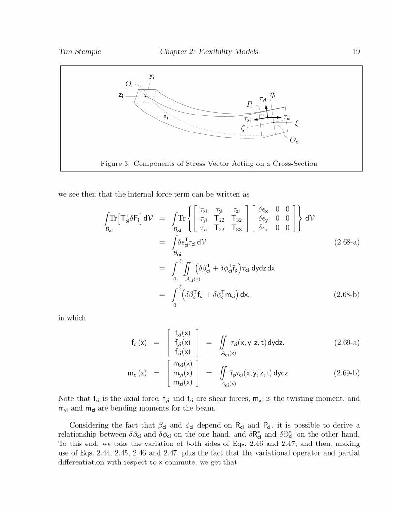
3 Components of Stress Vector Acting on a Cross-Section . . . . . . . . . . . . 19
4 Kinematical Relationship Between Body i and its Inboard Body j . . . . . . 39
5 Model of a Flexible Robot . . . . . . . . . . . . . . . . . . . . . . . . . . . . 55
6 Shape Functions for Bending . . . . . . . . . . . . . . . . . . . . . . . . . . . 56
7 Shape Functions for Torsion . . . . . . . . . . . . . . . . . . . . . . . . . . . 58
8 Actuator Pairs for Controlling Beam Vibrations . . . . . . . . . . . . . . . . 59
9 Time Histories of Robot Joint Angles . . . . . . . . . . . . . . . . . . . . . . 62
10 Time Histories of Beam Elastic Motions . . . . . . . . . . . . . . . . . . . . 63
11 Time Histories of Robot Joint Torques . . . . . . . . . . . . . . . . . . . . . 64
12 Time Histories of Elastic Torques . . . . . . . . . . . . . . . . . . . . . . . . 65
vi
Chapter 1 Introduction
1.1 Overview
The goal of this study is to present a method for deriving equations of motion capableof modeling the controlled motion of an open loop multibody structure comprised of anarbitrary number of rigid bodies and slender beams. The equations of motion for flexiblemultibody structures consist of simultaneous ordinary differential equations for the rigid-body motions and boundary-value problems, composed of partial differential equations andboundary conditions, for the elastic deformations. Such coupled sets of differential equationsare referred to as hybrid [33]. The solution of hybrid sets of equations is difficult, with theproblem further complicated by the fact that the equations are generally nonlinear, evenwhen the elastic deformations are small.
The procedure presented here for deriving equations of motion for flexible multibodysystems is carried out by means of the Principle of Virtual Work [31], often referred to inthe dynamics literature as d’Alembert’s Principle [32]. The Principle of Virtual Work allowsfor a fairly streamlined and systematic approach to the derivation of multibody dynamicsequations of motion. This is particularly true when the ultimate goal is to develop a generalpurpose computer program which can be applied to any number of different structures.
There are five basic steps involved in the derivation. In the first place we consider themotion of a general flexible body relative to the inertial space, and then derive specificformulas for both rigid bodies and slender beams. The slender beam equations, however, arenot in a form suitable for numerical analysis, so that the second step involves making a smallmotions assumption. This process includes a novel application of the exponential form of anorthogonal matrix, which is ideally suited for truncation, with the end result being equationsfor a Rayleigh beam [52]. In fact, the equations include terms which account for the axial
1
Tim Stemple Chapter 1: Introduction 2
motion, due to bending, of points on the beam central axis. The third step is to introducethe generalized coordinates and quasi-velocities used in the mathematical model, includingthose needed in the spatial discretization process of the beam equations. In the fourth stepwe discuss the relative motion of one body with respect to another and develop a new set ofrecursive relations used to compute the inertial motion of a body in terms of the generalizedcoordinates and quasi-velocities. In the fifth and final step, we combine the results of theprevious four steps to derive the system ordinary differential equations of motion used tomodel the multibody structure.
This research was motivated by the desire to model the controlled motion of a flexiblespace robot, such as the one used on the space shuttle. Consequently, we use the multibodydynamics equations to simulate the motion of such a structure, providing a demonstrationof the multibody dynamics code. For this particular example we make use of a sequenceof shape functions first used by Meirovitch and Stemple [46] to model a two dimensionalbuilding frame subjected to earthquake excitations. The results are presented in the formof plots of the various joint displacements, the displacements of points on the beams due tothe elastic motion, as well as the control torques of the various actuators.
1.2 Literature Survey
Many common engineering structures, including various types of spacecraft, land vehicles,industrial machinery and robots, can be modeled as multibody systems. The technicalliterature on the subject is vast, indeed, with publications going back several decades. Weinclude here a literature survey which represents a fair cross-section of all the various aspectsof multibody dynamic analysis.
In some applications multibody structures can be modeled by assuming that all bodiesin the structure are rigid, with the derivation of equations of motion carried out by a varietyof techniques such as Newton-Euler equations, d’Alembert’s principle, Lagrange’s equations,or the method popularized by Kane. The literature devoted to rigid multibody structures iswell established, and here we simply single out the books by Haug [17], Huston [20], Robersonand Schwertassek [51], Shabana [53] and Wittenburg [64], as well as papers by Kane andLevinson [22, 23].
The modeling of flexible multibody systems relies heavily on principles and techniques formodeling single flexible bodies. In an early paper, Meirovitch and Nelson [40] considered theproblem of stability of spinning spacecraft modeled as a rigid core with two flexible beamssimulating antennas. They derived Lagrange’s ordinary differential equations in terms ofquasi-coordinates for the rigid-body rotations of the core coupled with Lagrange’s partialdifferential equations for the elastic deformations relative to a reference frame embeddedin the rigid core. Using the concept of “floating reference frame,” de Veubeke [13] derivedequations of motion for a mean rigid body motion in terms of quasi-coordinates and modal
Tim Stemple Chapter 1: Introduction 3
equations for elastic motions measured relative to the mean rigid-body motion. Cavin andDusto [8] developed a variational formulation yielding finite element equations of motion fora single unconstrained elastic body. Using a Lagrangian approach, Meirovitch and Quinn [41]derived equations of motion for maneuvering flexible spacecraft. Then, they derived a setof perturbation equations with the rigid-body maneuvers as the unperturbed motion. Sha-bana [54] derived generalized Newton-Euler equations for deformable bodies undergoing largetranslational and rotational displacements. The equations were formulated in terms of time-invariant scalars and matrices depending on both spatial coordinates as well as the assumeddisplacement field. General hybrid equations of motion for an arbitrarily shaped body inspace were derived by Meirovitch [33], who extended the concept of quasi-coordinates totranslations in terms of body axes components. An example involving a flexible beam at-tached to a translating and rotating rigid disk was provided. Using Lagrange’s form ofd’Alembert’s principle, Weng and Greenwood [63] derived equations of motion for a bodyundergoing large elastic deformations, and then applied the formulation to a beam attachedto a rotating base. Zhang, Liu and Huston [68] used Kane’s equations to derive equations foroverall large motions of an arbitrarily shaped body. Two examples were provided, a rotatingbeam and a rotating plate.
Mathematical models for flexible multibody systems tend to be considerably more in-volved than those for single flexible bodies, or rigid bodies with flexible parts. Ho [18] usedthe “direct path method” to derive equations of motion for multibody spacecraft with topo-logical tree configuration, with the terminal bodies being flexible and the interconnectingbodies assumed to be rigid. Three methods for deriving the equations were considered,Lagrangian-Newtonian, all Newtonian and all Lagrangian. Vu-Quoc and Simo [61] consid-ered the dynamics of flexible multibody spacecraft by referring the motion to an inertialframe. To this end, they introduced a floating reference frame translating relative to theinertial space. Kim and Haug [25] used a recursive formulation to model the dynamics offlexible multibody systems, whereby the elastic deformation of each body is represented bydeformation modes. Two models for flexible multibody systems were considered by Yamada,Tsuchiya and Ohkami [65], one based on a Newton equation for each body in conjunctionwith constraint equations and one based on Kane’s equations. In the context of flexiblemultibody systems, Geradin, Cardona and Granville [15] discussed a nonlinear beam model,a substructuring technique for incorporating the flexibility of individual members into theoverall equations of motion and the incorporation of kinematic constraints. Chang andShabana [10] addressed the problem of modeling flexible multibody structures subjected tochanges in topology due to changes in the connectivity between bodies. They discretized thesystem by the finite element method. Extending the approach of Ref. [33], Meirovitch andKwak [37] considered the problem of pointing flexible antennas mounted on a spacecraft bystabilizing the spacecraft relative to the inertial space and maneuvering the antennas relativeto the spacecraft at the same time. Keat [24] developed an nth order algorithm capable ofmodeling systems of rigid or flexible bodies. The formulation can accomodate open-chain,tree and closed-loop topologies, and the joints connecting adjacent bodies can have 0 to 6 de-grees of freedom. A formulation of the dynamics of rotorcraft consisting of flexible and rigid
Tim Stemple Chapter 1: Introduction 4
components was presented by Agrawal [1]. The result of using the finite element method inconjunction with a multibody approach is a set of differential-algebraic equations of motion.Avello, de Jalon and Bayo [3] used Lagrange’s equations to derive equations of motion forflexible slender bodies modeled as nonlinear Timoshenko beams. Constraints are introducedwith a penalty formulation and the resulting differential equations were integrated by New-mark’s methods. Cyril, Angeles and Misra [12] developed a model consisting of both rigidand flexible links and used it to simulate a typical maneuver of the Space Shuttle remotemanipulator. Euler-Lagrange equations are derived for each body separately and then as-sembled to obtain the constrained dynamical equations for the multibody system. A newrecursive dynamics analysis of flexible multibody systems was formulated by Lai, Haug, Kimand Bae [28] using a kinematic graph concept and a variational vector calculus approach.Assuming small deformations, the flexibility was modeled by means of modal coordinates.To illustrate the approach, a flexible closed-loop spatial robot was analyzed. Nikravesh andAmbrosio [48] formulated the equations of motion for multibody systems containing bothrigid and flexible bodies. They used joint coordinates to derive the minimum number ofequations for the rigid bodies and the finite element method to discretize the flexible bodies.A systematic method for deriving the minimum number of equations of motion of spatialflexible multibody systems was presented by Pereira and Proenca [49]. Relative kinematicsin terms of relative joint coordinates and velocities was used to formulate the equations ofmotion. Shabana [55] considered issues related to the dynamics modeling of constrained de-formable bodies undergoing large rigid-body displacement. He discretized the bodies by thefinite element method. A formulation capable of treating the problem of maneuvering and vi-bration control of a flexible multibody system was developed by Kwak and Meirovitch [27].Equations of motion in terms of quasi-coordinates were derived for each body separatelyand then combined by means of a consistent kinematical synthesis. Vukasovic, Celiguetaand de Jalon [60] used Cartesian coordinates to model flexible multibody structures, withthe elastic deformations represented by linear combinations of Ritz vectors with respect toa local reference frame. An example involving a satellite deployment was provided. Variousissues in the structural modeling of flexible multibody systems were discussed by Suleman,Modi and Venkayya [57]. Comparative analyses between component and system modal dis-cretization techniques were presented. When the system undergoes large three-dimensionalrigid-body motions, in addition to elastic motions, Lagrange’s equations in terms of quasi-coordinates [32, 40, 50] provide an alternative to ordinary Lagrange’s equations [41]. Hybridequations of motion in terms of quasi-coordinates were derived by Meirovitch [34] directlyfrom Hamilton’s principle and by Meirovitch and Stemple [43] by transforming ordinary La-grange’s equations. The developments of Refs. [34] and [43] are carried out using symbolicvector operations in conjunction with recursive kinematical relations to eliminate redundantcoordinates. The hybrid equations have been discretized by Meirovitch and Stemple [42] bythe approach of Ref. [38] and the resulting ordinary differential equations cast in state formfor control.
The development of multibody dynamics formulations especially for modeling mecha-nisms and land vehicles has been made necessary to a large extent by the fact that the
Tim Stemple Chapter 1: Introduction 5
kinematics for such systems is substantially more complicated than for aerospace structures.In fact, the modeling of mechanisms and land vehicles often requires multibodies formingclosed loops, and in some cases even involves nonholonomic constraints. Because the inter-est in this paper lies mainly in aerospace structures and flexible robots, we concentrate thereview on a few papers in which the flexibility is included in the model.
Yoo and Haug [66, 67] developed a flexible multibody model in which the individual bod-ies can undergo large rigid-body motions but the elastic displacements remain small. Thedeformation modes for flexible bodies are generated by a lumped mass finite element ap-proach and the equations of motion are derived by using a Lagrange multipliers formulation.Koppens et. al. [26] considered the dynamics of a deformable body allowed to undergo largedisplacements, with the deformation modeled independently from the rigid-body motions bymeans of a linear combination of assumed displacement fields. The system equations of mo-tion were derived by d’Alembert’s principle and illustrated by means of a uniform beam anda crank-slider mechanism. Lieh [29] presented a separated-form formulation for the dynamicsand control of multibody systems with elastic members treated as Euler-Bernoulli beams,where “separated” is in the sense that the inertia matrix, nonlinear coupling vector, gener-alized force vector and base motion-induced terms are determined individually. Examplesinclude an elastic vehicle with active suspension and an elastic crank-slider mechanism. Theproblem of including the rotational, or dynamic stiffening, effect in the analysis of flexiblebodies has been considered by Wallrapp and Schwertassek [62].
Industrial robots have been modeled traditionally as chains of rigid bodies moving relativeto an inertial space, with adjacent bodies connected by motors providing internal controltorques. With the advent of lightweight industrial robots and space robots, such as the SpaceShuttle manipulator arm, it has become necessary to include the flexibility in the systemmodel.
Book et. al. [6] considered the control of a flexible robot consisting of two pinned beamsusing two flexibility models. They investigated and compared three types of linear feedbackcontrol. Later, Book [7] developed nonlinear equations of motion for flexible manipulatorarms with adjacent arms connected by rotary joints. Assuming small deformations, the dis-placement of the flexible links was expressed as linear combinations of shape functions. Theefficiency of the formulation was compared to that of a rigid-link model. Hughes [19] usedthe “direct path method” to derive equations of motion for a chain of bodies, with the twoend bodies being rigid and the intermediate bodies capable of small flexible motions. A com-puter program based on these dynamical equations was written and used to model the SpaceShuttle robot arm. Low [30] used Hamilton’s principle to derive hybrid equations of motionfor flexible robots including inertial, Coriolis, centrifugal, gravitational and external forceeffects. Two examples were studied, a three-link flexible manipulator with revolute jointsand a flexible manipulator consisting of a prismatic bar and a discrete mass. Naganathanand Soni [47] used a Newton-Euler formulation in conjunction with Timoshenko beam theorydiscretized by the finite element method to develop a nonlinear model capable of predicting
Tim Stemple Chapter 1: Introduction 6
the response of spatial manipulators with flexible links. From studies of both planar andspatial manipulators, they concluded that nonlinear kinematic coupling has significant effecton the positioning errors of the end-effector. Baruh and Tadikonda [4] used an approachsimilar to substructure synthesis to model a robot with elastic arms. They concluded thatthe centrifugal stiffening effect plays a large role in the overall system behavior. Bayo et.al. [5] considered the inverse dynamics and kinematics of multilink flexible robots, with thelinks modeled by the Timoshenko beam theory discretized by the finite element method.A method was developed for determining the joint torques required to produce a specifiedend-effector motion, with the performance tested both by simulation and experiment. Equa-tions of motion for a planar model of the proposed Space Station-based Mobile ServicingSystem were derived by means of Lagrange’s equations by Chan and Modi [9], who designedcontrols using linear quadratic theory. A parallel processing algorithm to simulate the dy-namical equations for constrained flexible multibody systems undergoing large rotations wasdeveloped by Ider [21], who tested its performance by simulating a spatial robotic manip-ulator. Amirouche and Xie [2] used Kane’s equations to develop a model for the dynamicsimulation of rigid/flexible multibody systems. Using finite element discretization, a recur-sive formulation was developed and applied to a two-link robot manipulator. Meirovitchand Lim [39] considered the controlled response of a flexible space robot. A perturbationapproach applied to the original nonlinear equations of motion permitted the control law tobe divided into two parts, one for rigid-body maneuvering carried out open-loop and anotherfor the elastic motions controlled by a closed-loop discrete-time linear quadratic regulatorwith prescribed degree of stability. Meirovitch and Chen [36] considered the problem ofdesigning controls for a flexible space robot required to ferry a payload in space and to dockwith an orbiting target. The robot trajectory is determined by an optimization procedure,with controls based on a perturbation approach. The rigid-body maneuvering control is de-termined using inverse dynamics and the elastic vibration is controlled by a linear quadraticregulator for time-varying systems. Chen and Meirovitch [11] developed a control schemefor a docking maneuver of a flexible space robot with a moving target. The problem iscomplicated by the assumption that the target’s motion is not known a priori. Lagrange’sequations are used to derive equations of motion, which are separated into two sets suitablefor rigid-body maneuver and vibration suppression control. Van Woerkom and de Boer [59]developed an “order-n” algorithm used to simulate the motion of a flexible space manipula-tor consisting of a base (the spacecraft) and an end-effector connected by a chain of flexiblearms. A discussion of the parametric Lagrange form of d‘Alembert’s principle is included.Van Woerkom [58] discussed the problem of including the axial deformation of beams, asapplied to models of space robots. Four methods of including the axial deformation, i.e.,nonlinear deformation field modeling, perturbed dynamics modeling, fictitious joints model-ing and bracket joints modeling, are discussed. The hybrid equations of Refs. [34] and [43]were first discretized by means of substructure synthesis [38] and then used by Meirovitchand Stemple [42, 44, 45] to carry out rest-to-rest maneuvers of flexible robots. Controls weredesigned by the Liapunov direct method and direct feedback control was used to suppressthe elastic vibration of the links.
Chapter 2 Flexibility Models
In this chapter we develop the equations required to describe the inertial kinematics anddynamics of the bodies making up the structure. Vectors and tensors in three-dimensionalEuclidian space are denoted with bold type (R, u, F, Ω), points are denoted with italic type
−−→(O , P , P ) and, as usual, the notation P P represents a vector with initial point P ando 1 2 1 2 1
terminal point P . Scalars and matrices are denoted by plane type (R, u, F, Ω) with the23 T T Tusual basis in R given by e = [1 0 0] , e = [0 1 0] and e = [0 0 1] . The terminology1 2 3
component matrix refers to either a 3-by-1 matrix, r for example, containing the componentsof a vector r along specified orthogonal axes, or a 3-by-3 matrix, F for example, containingthe components of a tensor F with respect to specified orthogonal axes. Furthermore, we letO; xyz stand for an orthogonal coordinate system with axes xyz and origin O. Some basicmatrix definitions and identities are developed in the Appendix.
2.1 Principle of Virtual Work
The starting point for deriving equations of motion is the Principle of Virtual Work [31],which, for a structure comprised of N bodies labeled i = 1, 2, . . . , N, takes the form
N∑R = 0, (2.1)i
i=1
where a general expression for R valid for any model of a solid body is given byi∫ ∫ [ ]¨R = ρ (r )z · δz (r , t) dV + Tr T (r , t)δF (r , t) dVi oi i i i i oi i i i
B Boi oi∫ ∫− b (r , t) · δz (r , t) dV − τ (r , t) · δz (r , t) dA. (2.2)oi i i i oi i i i
B ∂Boi oi
7
Tim Stemple Chapter 2: Flexibility Models 8
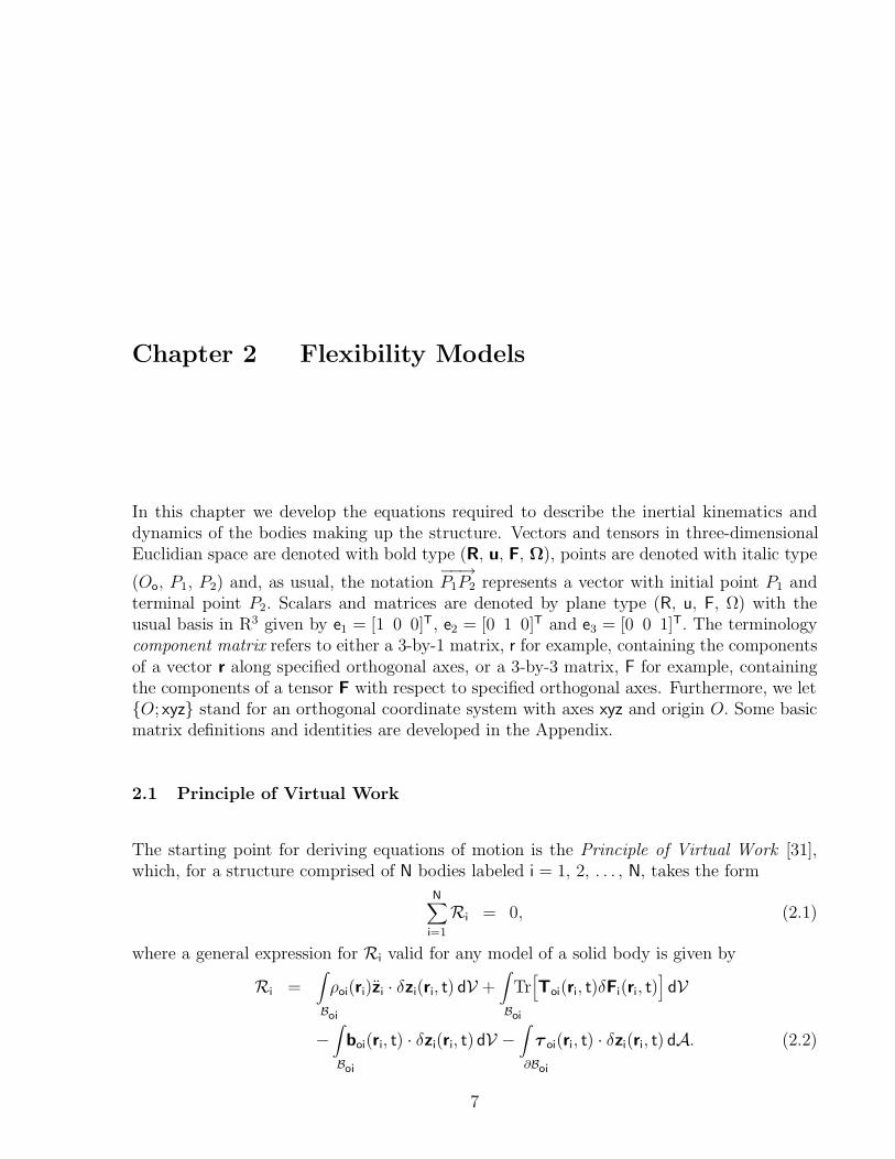
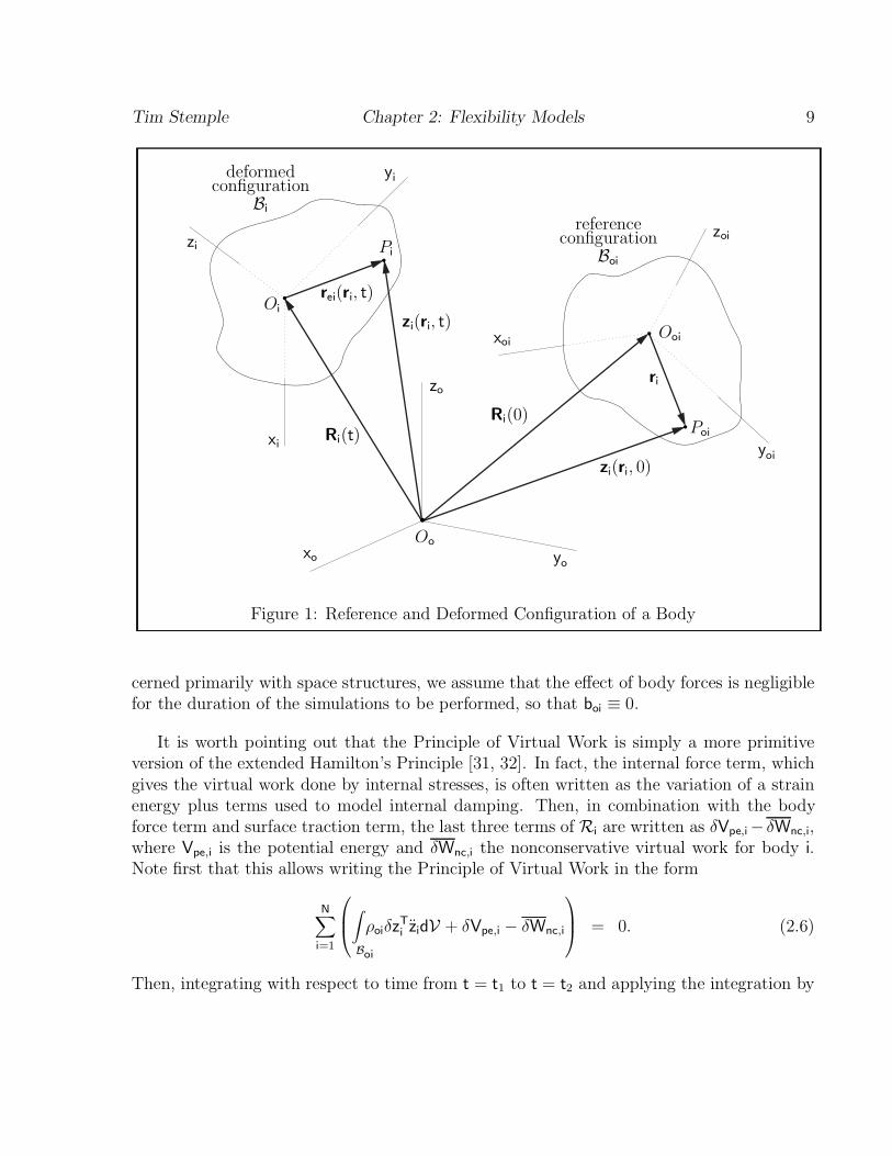
This is where the region B , which serves as a reference configuration for body i, is occupiedoi −−−→by the body at time t = 0, and ∂B is the boundary of B (Fig. 1). Furthermore, r = O Poi oi i oi oi
is the position vector of a typical point P in B , ρ (r ) is the mass density of the body, whenoi oi ci i
in the reference configuration, T (r , t) is the (first) Piola-Kirchoff stress tensor for body i,oi i
and b (r , t) and τ (r , t) are, respectively, the body force density (force per unit referenceoi i oi i
volume) and surface traction (force per unit reference surface area). As the bodies in thestructure translate, rotate and deform, the points O and P of body i will occupy newoi oi
points in space, which we denote by O and P , respectively. To keep track of the position ofi i−−→ −−→points O and P , we let R (t) = O O and z (r , t) = O P , where O is a point fixed in thei i i o i i i o i o
inertial space. The gradient of z (r , t) with respect to r , denoted by F (r , t) = ∇z (r , t), isi i i i i i i
a second order tensor referred to as the deformation gradient [16] of body i.
Although we could proceed with the derivation directly from Eq. 2.2, it is more efficientto first rewrite the formula for R in terms of vector and tensor components. To this end,i
we introduce the inertial coordinate system O ; x y z (Fig. 1) and the moving coordinateoo o o
system O ; x yz , fixed on body i, for i = 1, 2, . . . , N; body axes x y z , for time t = 0, arei ii i i i iTdenoted by x y z . Then, r = [x y z] denotes the component matrix of vector r , alongoioi oi i i
axes x y z , R (t) and z (r , t) = z (x, y, z, t) are component matrices for vectors R (t) andoioi oi i i i i i
z (r , t), respectively, both along inertial axes x y z , and r (r , t) is the component matrix,oi i o o ei i−−→
along body axes x y z , for vector r (r , t) = O P , implying that r (r , 0) = r . Note that theii i ei i i i ei i i
components of r are Lagrangian (or material) coordinates and the components of z arei i
Eulerian (or spatial) coordinates for body i. We also let T , F , b and τ be the componentoi i oi oi
matrices of T , F , b and τ , respectively, all with components along inertial axes x y z .ooi i oi oi o o
The component matrix T of the Piola-Kirchoff stress tensor, which measures force per unitoi
area in the reference configuration, is related to T , the component matrix (also with respectci
to inertial axes x y z ) of the Cauchy stress tensor, by the formula [16]oo o
−TT = (det F )T F . (2.3)oi i ci i
Recall that the conservation of angular momentum principle implies that the Cauchy stresstensor is symmetric, that is,
TT = T . (2.4)cici
Then, since z , T , F , b and τ are all in terms of components along the same set ofi oi i oi oi
axes, we can rewrite Eq. 2.2 in the form∫ ∫ [ ]TT ¨R = ρ (r )δz (r , t)z (r , t) dV + Tr T (r , t)δF (r , t) dVi oi i i i i i i ii oi
B Boi oi∫ ∫T T− δz (r , t)b (r , t) dV − δz (r , t)τ (r , t) dA. (2.5)i oi i i oi ii i
B ∂Boi oi
The four terms making up R will be referred to, in order, as the inertia term, the internali
force term, the body force term and the surface traction term. However, since we are con-
Tim Stemple Chapter 2: Flexibility Models 9
deformed yiconfiguration
Bi
reference zoiconfigurationzi Pi Boi
r (r , t)ei iOi
z (r , t)i i Ooixoi
rizo
R (0)iPoiR (t)ixi yoi
z (r , 0)i i
Ooxo yo
Figure 1: Reference and Deformed Configuration of a Body
cerned primarily with space structures, we assume that the effect of body forces is negligiblefor the duration of the simulations to be performed, so that b ≡ 0.oi
It is worth pointing out that the Principle of Virtual Work is simply a more primitiveversion of the extended Hamilton’s Principle [31, 32]. In fact, the internal force term, whichgives the virtual work done by internal stresses, is often written as the variation of a strainenergy plus terms used to model internal damping. Then, in combination with the bodyforce term and surface traction term, the last three terms of R are written as δV − δW ,i pe,i nc,i
where V is the potential energy and δW the nonconservative virtual work for body i.pe,i nc,i
Note first that this allows writing the Principle of Virtual Work in the form ∫N∑ T¨ρ δz z dV + δV − δW = 0. (2.6) oi i pe,i nc,iii=1 Boi
Then, integrating with respect to time from t = t to t = t and applying the integration by1 2
Tim Stemple Chapter 2: Flexibility Models 10
parts formula yields the extended Hamilton’s Principle,
∫ t2
(δL + δW ) dt = 0, (2.7)nct1
δz (r , t ) = δz (r , t ) = 0, r ∈ B , i = 1, 2, . . . ,N, (2.8)i i 1 i i 2 i oi
whereL = T− V (2.9)
is the system Lagrangian, in which
∫N∑1 T˙ ˙T = ρ r r dV (2.10)oi ii2 Boii=1
is the kinetic energy of the system,
N∑V = V (2.11)pe pe,i
i=1
is the potential energy andN∑
δW = δW (2.12)nc nc,i
i=1
is the system nonconservative virtual work.
2.2 Rigid Body Motion
The motion of coordinate system O ; x y z with respect to coordinate system O ; x y z i oi i i o o o
involves both the translation of point O as well as the rotation of axes x y z . We have earlierii i i
introduced the component matrices R (t) and z (r , t), which involve the position of points Oi i i i
and P , respectively, with respect to the inertial space. We also require the matrix of directioni
cosines of body axes x y z relative to the inertial axes x y z , which is denoted by P (t). Notei oi i o o iTthat since P (t) transforms components of a vector, along axes x yz , to components of theii i i
same vector, but along axes x y z , the matrix form of the vector equation (Fig. 1)oo o
z (r , t) = R (t) + r (r , t) (2.13)i i i ei i
is given byTz (r , t) = R (t) + P r (r , t). (2.14)i i i i ei i
We also make use of the quasi-velocities V (t) and Ω (t), which are, respectively, componenti i˙matrices, along axes x y z , for the velocity vector R (t), and angular velocity vector Ω (t) ofii i i i
Tim Stemple Chapter 2: Flexibility Models 11
axes x yz with respect to axes x y z . Referring to Eqs. A.24 and A.25 in the appendix, thisi oi i o o
implies that
˙V = P R , (2.15)i i i
T˜ ˙Ω = P P . (2.16)i i i
∗∗Analogous to V and Ω , the quasi-virtual displacements δR and δΘ are defined byi i ii
∗δR = P δR , (2.17)i ii
∗ TδΘ = P δP , (2.18)i i i
and, due to the fact that P (t) is an orthogonal matrix, Eqs. 2.16 and 2.18 can be rewritteni
in the forms ˜P = −Ω P , (2.19)i i i
T T˜P = P Ω , (2.20)i i i
∗˜δP = −δΘ P , (2.21)i i i
∗T T ˜δP = P δΘ . (2.22)i i i
At this point we derive a formula for F (r , t), which was introduced earlier as the compo-i i
nent matrix, with respect to inertial axes x y z , of the deformation gradient ∇z of body i.oo o i
Note first that the constant matrix P (0) is the matrix of direction cosines of axes x y zoii oi oiT¯ ¯with respect to axes x y z . Then, by definition [16], F = ∂z /∂r , in which r = P (0)r is theoo o i i i i i i
component matrix, along axes x y z , of position vector r . Referring now to Eq. A.39 andoo o i
the comment immediately preceding it, we see that
∂z (r , t)i iF (r , t) = P (0). (2.23)i i iT∂ri
The equations developed so far in this section are valid for any of the bodies in thestructure. However, for the time being at least, we proceed with the assumption that body iis rigid. This means that the distance between any two points in the body remains constant,which, when applied to points O and P (Fig. 1), implies thati i
r (r , t) = r . (2.24)ei i i
Substituting this into Eq. 2.14, the component matrix, along inertial axes x y z , for theoo o
position vector of an arbitrary point in a rigid body is given by
Tz = R + P r . (2.25)i i i i
Recalling that r is independent of time, so that r = 0, we take time derivatives of Eq. 2.25i i
and make use of Eqs. 2.15 and 2.20 to get that
T˜˙z = R + P Ω ri i i i i
T ˜= P (V − r Ω ), (2.26)i i i i
T T˜˙ ˙z = P (V − r Ω ) + P Ω (V − r Ω )i i i i i i i i i i
T ˜ ˜˙ ˙˜ ˜= P (V − r Ω + Ω V − Ω r Ω ). (2.27)i i i i i i i i i
Tim Stemple Chapter 2: Flexibility Models 12
Then, analogous to Eq. 2.26, we take the variation of Eq. 2.25 and use Eqs. 2.17 and 2.22to get that
∗T˜δz = δR + P δΘ ri i i i i
∗∗T ˜= P (δR − r δΘ ). (2.28)i i ii
Considering now the deformation gradient for the body, Eqs. 2.23, 2.25 and A.5 imply that
T∂z ∂(R + P r )i i i i TF = P (0) = P (0) = P P (0). (2.29)i i i i iT T∂r ∂ri i
Furthermore, we can use Eq. 2.22 to get the variation of the deformation gradient as
∗T˜δF = P δΘ P (0), (2.30)i i i i
and also, since P and P (0) are both proper orthogonal matrices, F is also proper orthogonal,i i i
so thatdet F = 1. (2.31)i
We now have enough information to construct the formula for R . Substituting Eqs. 2.27i
and 2.28 into Eq. 2.5 and making use of Eq. A.11, the inertia term for a rigid body takesthe form ∫ ∫ ( ) ( )
∗T∗TT T ˜ ˜˙ ˙ρ δz z dV = ρ δR + δΘ r P P V − r Ω + Ω V − Ω r Ω dVoi i oi i i i i i i i i i i i ii i
B Boi oi ( )∗T ˜ ˜ ˜ ˜˙ ˙= δR m V − S Ω + Ω V −Ω S Ωi i ei i i i i ei ii ( )∗T ˜ ˜ ˜ ˜˙ ˙+ δΘ S V + J Ω + S Ω V + Ω J Ω , (2.32)i ei i ei i ei i i i ei i
in which ∫m = ρ (r ) dV, (2.33-a)i oi i
Boi∫S = ρ (r )r dV, (2.33-b)ei oi i i
Boi∫T˜˜J = ρ (r )r r dV, (2.33-c)ei oi i i i
Boi
(2.33-d)
are the mass, first moments of inertia, and mass moments of inertia, respectively, for thebody. Next, substituting Eqs. 2.3, 2.29 and 2.30 into Eq. 2.5, and making use of Eqs. A.37,
Tim Stemple Chapter 2: Flexibility Models 13
2.4 and 2.31, the internal force term for a rigid body takes the form∫ ∫[ ] [ ]∗T −1 T˜Tr T δF dV = Tr (det F )F T P δΘ P (0) dVi i ci i i ioi i
B Boi oi∫ [ ]∗T T˜= Tr P (0)P T P δΘ P (0) dVi i ci i i i
Boi∫ [ ]∗ T T˜= Tr δΘ P (0)P (0)(P T P ) dVi i i i ci i
Boi∫ [ ]∗ T˜= Tr δΘ (P T P ) dV = 0, (2.34)i i ci i
Boi
∗˜where the last equality follows from Eq. A.38 and the fact that δΘ is skew-symmetric andiTP T P is symmetric.i ci i
We consider now the surface traction term. In this regard, first note that the surfacetraction τ can be written asoi
∗ Tτ = τ + P τ , (2.35)oi i sioi
∗where τ is nonzero only on that part of the surface of body i which contacts another bodyoi
in the structure, and τ is nonzero only on that part of the surface of body i which doessiTnot contact any other body in the structure. Note that including P in this formula impliesi
that τ is in terms of components along body axes x y z . Then, substituting into Eq. 2.5 andisi i i
making use of Eq. 2.28, we get that∫ ∫ ∫ ( )∗T∗TT T ∗ Tδz τ dA = δz τ dA+ δR + δΘ r P P τ dAoi i i i i sii i oi i
∂B ∂B ∂Boi oi oi∫∗T∗TT ∗= δz τ dA+ δR F + δΘ M , (2.36)si i sii oi i
∂Boi
where ∫F (t) = τ (r , t) dA, (2.37-a)si si i
∂Boi∫M (t) = r τ (r , t) dA, (2.37-b)si i si i
∂Boi
are external force and moment component matrices, both along body axes x y z . Now combineii i

Tim Stemple Chapter 2: Flexibility Models 14
Eqs. 2.32, 2.34 and 2.36, plus the fact that the body force is assumed to be zero, to get that( [ ] ) ∫[ ] Vi∗T∗T T ∗R = M − G − δz τ dA, (2.38)δR δΘi rri rii i oii Ωi∂Boi
where [ ]˜m I −Si eiM = , (2.39-a)rriS Jei ei[ ] [ ] [ ]˜ ˜ ˜−m Ω Ω S V Fi i i ei i siG = + . (2.39-b)ri ˜ ˜ ˜ Ω M−S Ω −Ω J i siei i i ei
2.3 Slender Beams
The reference configuration B for a slender beam can be written in the form [52]oi
B = (x, y, z)|(y, z) ∈ A (x) for 0 ≤ x ≤ ` , (2.40)oi ci i
2where ` is the length of the beam and A (x) ⊆ R defines a cross-section. We make thei ci
common simplifying assumption that cross-sections remain planar, which allows the intro-duction of an orthogonal coordinate system O ; ξ η ζ (Fig. 2) fixed on cross-section A (x).ci i i i ci
We also assume that the ξ -axis coincides with the central axis of the beam in undeformedi
state, and that body axes x y z coincide with cross-section axes ξ η ζ at x = 0.ii i i i i
We start by considering the motion of points in cross-section A (x) relative to the inertialci
space. In fact, due to the assumption that cross-sections remain planar, the analysis isessentially the same as for a rigid body. To this end, R (x, t) denotes the component matrix,ci
−−−→along inertial axes x y z , of position vector R (x, t) = O O (Fig. 2) and P (x, t) is theoo o ci o ci ci
matrix of direction cosines of cross-section axes ξ η ζ with respect to inertial axes x y z .oi i i o o˙Furthermore, V (x, t) is the component matrix of velocity vector R (x, t) and Ω (x, t) isci ci ci
the component matrix of the angular velocity vector, Ω (x, t), of axes ξ η ζ with respect toci i i i
axes x y z , both with components along cross-section axes ξ η ζ . We also make use of quasi-oo o i i i∗∗virtual displacements analogous to V (x, t) and Ω (x, t), denoted by δR (x, t) and δΘ (x, t),ci ci cici
respectively, and letTr = [0 y z] (2.41)p
−−→be the component matrix, along cross-section axes ξ η ζ , of vector O P , where P is a pointi i i ci i i
in the beam with Lagrangian coordinates (x, y, z).
Tim Stemple Chapter 2: Flexibility Models 15
ηi
yi ξir (x, t)ci
ζi
xiOi Oci
zo
zi R (x, t)ci
R (t)i
yoOo
xo
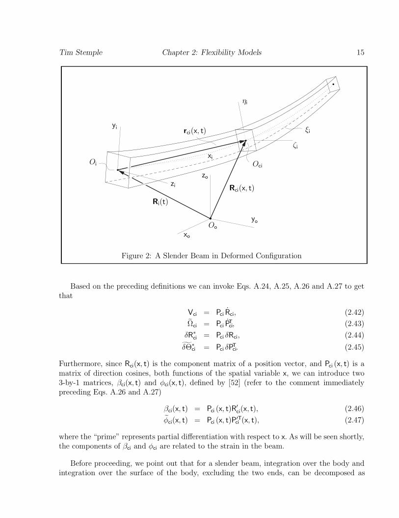
Figure 2: A Slender Beam in Deformed Configuration
Based on the preceding definitions we can invoke Eqs. A.24, A.25, A.26 and A.27 to getthat
˙V = P R , (2.42)ci ci ci
T˜ ˙Ω = P P , (2.43)ci ci ci
∗δR = P δR , (2.44)ci cici
∗ TδΘ = P δP . (2.45)ci ci ci
Furthermore, since R (x, t) is the component matrix of a position vector, and P (x, t) is aci ci
matrix of direction cosines, both functions of the spatial variable x, we can introduce two3-by-1 matrices, β (x, t) and φ (x, t), defined by [52] (refer to the comment immediatelyci ci
preceding Eqs. A.26 and A.27)
′β (x, t) = P (x, t)R (x, t), (2.46)ci ci ci
′Tφ (x, t) = P (x, t)P (x, t), (2.47)ci ci ci
where the “prime” represents partial differentiation with respect to x. As will be seen shortly,the components of β and φ are related to the strain in the beam.ci ci
Before proceeding, we point out that for a slender beam, integration over the body andintegration over the surface of the body, excluding the two ends, can be decomposed as
Tim Stemple Chapter 2: Flexibility Models 16
follows: ∫ ∫ ∫∫`i
dV = dydz dx, (2.48-a)
B 0 A (x)oi ci∫ ∫ ∮`idA = ds dx, (2.48-b)
∂B 0 ∂A (x)oi ci
where s measures arc length around the boundary of cross-section A (x).ci
Because of the assumption that a beam cross-section translates and rotates as a thinrigid plate, we can make use of the rigid body derivations and substitute r and R for r andp ci i
∗∗ ∗R , respectively, in Eq. 2.25, and then substitute V , Ω , δR and δΘ for V , Ω , δR andi ci ci ci i ici i∗δΘ , respectively, in Eqs. 2.25, 2.26, 2.27 and 2.28 to arrive ati
Tz = R + P r , (2.49)i ci ci p( )T˙ ˜z = P V − r Ω , (2.50)i ci ci p ci( )T ˜ ˜˙ ˙¨ ˜ ˜z = P V − r Ω + Ω V − Ω r Ω , (2.51)i ci ci p ci ci ci ci p ci( )
∗∗Tδz = P δR − r δΘ . (2.52)i ci p cici
To derive a formula for the inertia term, combine Eqs. 2.51 and 2.52, and then make use ofEq. 2.48-a to get that ∫ ∫ ∫∫` ( ) ( )i ∗TT ∗T T ˜ ˜˙ ˙¨ ˜ ˜ ˜ρ δz z dV = ρ δR + δΘ r P P V − r Ω + Ω V − Ω r Ω dydz dxoi i oi ci p ci ci ci p ci ci ci ci p cii ci
B 0 A (x)oi ci∫ ∫∫` [ ( )i ∗T ˜ ˜˙ ˙˜ ˜ρ δR V − r Ω + Ω V − Ω r Ωoi ci p ci ci ci ci p cici
0 A (x)ci ( )]∗T 2 2˜ ˜˙ ˙˜ ˜ ˜ ˜+δΘ r V − r Ω + r Ω V − Ω r Ω dydz dxci p ci ci p ci ci ci cip p∫ ` [ ( ) ( )]i ∗∗T ˜ ˜˙ ˆ ˙ ˆ= δR ρ V + ρ Ω V + δΘ J Ω + Ω J Ω dx, (2.53)ci ci ci ci ci ci ci ci ci ci cici
0
where ∫∫ρ (x) = ρ (x, y, z) dydz (2.54)ci oi
A (x)ci
is the mass per unit length, ∫∫Tˆ ˜ ˜J (x) = ρ (x, y, z)r r dydzci oi p p
A (x)ci [ ]ˆ ˆ ˆ= diag J (x), J (x), J (x) (2.55)xxi yyi zzi
Tim Stemple Chapter 2: Flexibility Models 17
is the mass moment of inertia density, with∫∫2J (x) = ρ (x, y, z)z dydz, (2.56-a)yyi oi
A (x)ci∫∫2J (x) = ρ (x, y, z)y dydz, (2.56-b)zzi oi
A (x)ci
ˆ ˆ ˆJ (x) = J (x) + J (x), (2.56-c)xxi yyi zzi
and we have assumed that each cross-section is symmetric, implying that∫∫ρ (x, y, z)r dydz = 0. (2.57)oi p
A (x)ci
For future use, we also define [ ]∗ ˆ ˆJ (x) = diag 0, J (x), J (x) , (2.58)zzi yyici
and note that∗ˆ ˆJ + J = J I, (2.59)ci xxici
in which I is the 3-by-3 identity matrix.
To derive a formula for the deformation gradient we make use of Eqs. 2.23, 2.41, 2.46,2.47 and 2.49 to get that
. .[ ]. . [ . . ]. .∂z ∂z ∂z ∂z . .. .i i i i ′ . .T T T. . ˜ . .. .F = P (0) = P (0) = R + P φ r P e P e P (0)i i i ci ci p ci 2 ci 3 i. .. . ciT . .. .∂r ∂x ∂y ∂z. .i . .[ . . ] [ . . ]. . . .. . . .T T. . . .˜= P β − r φ e e P (0) = P ε + e e e P (0)ci ci p ci 2 3 i ci ci 1 2 3 i. . . .. . . . ε + 1 0 0xi T= P ε 1 0 P (0) (2.60-a) yici i
ε 0 1zi
TT= P (ε e + I)P (0), (2.60-b)ci ci i1
in which the component matrix of a strain vector for the body is defined by ε (r , t)xi i ε (r , t) ˜ε (r , t) = = β (x, t)− e − r φ (x, t). (2.61) ci i yi i ci 1 p ci
ε (r , t)zi i
Now take the variation of Eq. 2.60-b, and then use Eqs. A.29 and 2.45 to get that( ) ( )∗ T TT T˜δF = P δΘ ε e + I P (0) + P δε e P (0)i ci ci ci i ci ci i1 1( ) ( )
∗ TT T= Tilde P δΘ F + P δε e P (0). (2.62)ci ci i ci ci i1
Tim Stemple Chapter 2: Flexibility Models 18
Furthermore, we can use Eq. 2.60-a to arrive at the formulas
det F = ε + 1, (2.63)i xi 1 0 0 −1 T(det F )F = P (0) −ε 1 + ε 0 P . (2.64) yi xii i cii
−ε 0 1 + εzi xi
Consequently, making use of Eqs. A.37, A.38, 2.3, 2.4, 2.62 and 2.64, the internal force termtakes the form∫ ∫ [ ]
T −1Tr[T δF ] dV = Tr (det F )F T δF dVi i ci ioi i
B Boi oi∫ [ ( ) ( ) ]∗−1 TT T= Tr (det F )F T Tilde P δΘ F + P δε e P (0) dVi ci ci ci i ci ci ii 1
Boi∫ [ ( ) ]∗ −1T= Tr (det F )Tilde P δΘ F F T dVi ci ci i cii
Boi 1 0 0∫ ( ) TT T+ Tr P (0) −ε 1 + ε 0 P T P δε e P (0) dV yi xii ci ci ci ci i1 −ε 0 1 + εB zi xioi δε 0 0 1 0 0∫ xi ( ) T Tδε 0 0 −ε 1 + ε 0= Tr P T P P (0)P (0) dV. ci ci ci yi i i yi xi δε 0 0 −ε 0 1 + εB zi zi xioi
(2.65)
TNow take note that P T P is the component matrix, with respect to cross-section axes ξ η ζ ,ci ci ci i i i
of the Cauchy stress tensor, and let τ (r , t)xi i τ (r , t) = τ (r , t) (2.66) ci i yi i
τ (r , t)zi i
be the component matrix, along cross-section axes ξ η ζ , for the stress vector acting on thei i i
cross-section A (x), as shown in Fig. 3. Recall from basic continuum mechanics [16] thatci
since the ξ -axis is perpendicular to the cross-section, τ is both the first row and first columni ciTof component matrix P T P . This allows writingci ci ci
τ τ τxi yi zi TP T P = τ T T , (2.67) yi 22 32ci ci ci
τ T Tzi 32 33
in which T , T and T are stress tensor components which enforce the “cross-sections re-22 32 33
main planar” assumption. Continuing from Eq. 2.65, and making use of Eqs. 2.48-a and 2.61,
Tim Stemple Chapter 2: Flexibility Models 19
yi
Oi
ηz ii τyiPi
x τi xiτzi ξiζi
Oci
Figure 3: Components of Stress Vector Acting on a Cross-Section
we see then that the internal force term can be written as τ τ τ δε 0 0∫ ∫ xi yi zi xi [ ] TTr T δF dV = Tr τ T T δε 0 0 dV yi 22 32 yiioi τ T T δε 0 0B B zi 32 33 zioi oi∫T= δε τ dV (2.68-a)cici
Boi∫ ∫∫` ( )iT T= δβ + δφ r τ dydz dxp cici ci
0 A (x)ci∫ `( )iT T= δβ f + δφ m dx, (2.68-b)ci cici ci
0
in which f (x) ∫∫xi f (x)f (x) = = τ (x, y, z, t) dydz, (2.69-a) ci yi ci
f (x) A (x)zi ci m (x) ∫∫xi ˜m (x) = m (x) = r τ (x, y, z, t) dydz. (2.69-b) ci yi p ci
m (x) A (x)zi ci
Note that f is the axial force, f and f are shear forces, m is the twisting moment, andxi yi zi xi
m and m are bending moments for the beam.yi zi
Considering the fact that β and φ depend on R and P , it is possible to derive aci ci ci ci∗ ∗relationship between δβ and δφ on the one hand, and δR and δΘ on the other hand.ci ci cici
To this end, we take the variation of both sides of Eqs. 2.46 and 2.47, and then, makinguse of Eqs. 2.44, 2.45, 2.46 and 2.47, plus the fact that the variational operator and partialdifferentiation with respect to x commute, we get that
Tim Stemple Chapter 2: Flexibility Models 20
′ ′δβ = (δP )R + P δRci ci cici ci
∗ ′ ′ ′˜= −δΘ P R + (P δR ) − P δRci ci ci ci ci cici
∗ ∗′˜ ˜= −δΘ β + δR + φ P δRci ci ci ci cici∗′ ∗ ∗˜ ˜= δR + φ δR + β δΘ , (2.70)ci ci cici ci
′T ′Tδφ = (δP )P + P δPci ci ci cici′∗ ′T T ′ T˜= −δΘ P P + (P δP ) − P δPci ci ci ci ci ci ci
∗ ∗′ T˜ ˜ ˜ ˜= −δΘ φ + δΘ + φ P δPci ci ci ci ci ci
∗′ ∗ ∗˜ ˜ ˜ ˜ ˜= δΘ + φ δΘ − δΘ φci ci ci ci ci˜∗′ ∗˜ ˜= δΘ + (φ δΘ ), (2.71)ci ci ci
where the last equality follows from Eq. A.10. Equation 2.71 then implies that
∗′ ∗˜δφ = δΘ + φ δΘ . (2.72)ci ci ci ci
We turn now to the surface traction term. As with the rigid body case, we can split τoi
into two parts,∗ Tτ = τ + P τ , (2.73)oi ci sioi
∗where τ is nonzero only on that part of the surface of body i which contacts another bodyoi
in the structure, which in this case means one or both ends of the beam, and τ is nonzerosi
only on that part of the surface of body i which does not contact any other body in theTstructure. Note that including P in this formula implies that τ is in terms of componentsci si
along cross-section axes ξ η ζ . Then, making use of Eqs. 2.48-b and 2.52, we get thati i i∫ ∫ ∫ ∮` ( )i ∗TT T ∗ ∗T T˜δz τ dA = δz τ dA+ δR + δΘ r P P τ ds dxoi ci p ci ci sii i oi ci
∂B ∂B 0 ∂A (x)oi oi ci∫ ∫ `( )i ∗TT ∗ ∗Tˆ ˆ= δz τ dA+ δR f + δΘ m dx, (2.74)si ci sii oi ci
∂B 0oi
where f (x, t) ∮xi ˆ ˆf (x, t) = = τ (x, y, z, t) ds, (2.75-a)f (x, t)si siyi ˆ ∂A (x)f (x, t)zi ci m (x, t) ∮xi ˆ ˆ ˜m (x, t) = m (x, t) = r τ (x, y, z, t) ds, (2.75-b) yisi p si
m (x, t) ∂A (x)zi ci
are surface force and moment component matrices, respectively, which can be used to accountboth for forces acting along the length of the beam, as well as forces and moments externalto the structure as a whole acting at the ends of the beam.
Tim Stemple Chapter 2: Flexibility Models 21
Now combine Eqs. 2.53, 2.68-b, 2.70, 2.72 and 2.74, plus the assumption that body forcesare zero, with Eq. 2.5, to get that
∫ ` [ ( ) ( )i ∗T ∗T˜ ˜˙ ˆ ˆ ˙ ˆ ˆR = δR ρ V + ρ Ω V − f + δΘ J Ω + Ω J Ω −mi ci ci ci ci ci si ci ci ci ci ci ci sici
0 ∫]T T T ∗+δβ f + δφ m dx− δz τ dA (2.76-a)ci cici ci i oi
∂Boi∫ ` [ ( ) ( )i ∗T∗T ˜ ˜˙ ˆ ˆ ˆ˙= δR ρ V + ρ Ω V − f + δΘ J Ω + Ω J Ω − mci ci ci ci ci si ci ci ci ci ci ci sici
0 ∫( ) ( ) ]∗′T ∗T ∗T ∗′T ∗T T ∗˜ ˜ ˜+ δR − δR φ − δΘ β f + δΘ − δΘ φ m dx− δz τ dAci ci ci ci ci ci ci cici ci i oi
∂Boi∫ ` [ ( ) ( )i ∗T ∗T˜ ˜ ˜˜ ˜˙ ˆ ˆ ˙ ˆ ˆ= δR ρ V +ρ Ω V −φ f − f + δΘ J Ω + Ω J Ω − β f −φ m −mci ci ci ci ci ci ci si ci ci ci ci ci ci ci ci ci ci sici
0 ∫]∗′T∗′T T ∗+δR f + δΘ m dx− δz τ dA (2.76-b)ci ci cici i oi
∂Boi∫ ` [ ( ) (i ∗T∗T ′ ′˜ ˜ ˜ ˜˙ ˆ ˆ ˆ˙= δR ρ V + ρ Ω V − f − φ f − f + δΘ J Ω + Ω J Ω −m − β fci ci ci ci ci ci ci si ci ci ci ci ci ci ci cici ci ci
0 ∫∣)] ( ) `i∣∗T∗T T ∗˜ ˆ−φ m −m dx + δR f + δΘ m ∣ − δz τ dA, (2.76-c)ci ci si ci ci cici i oi0∂Boi
where the last equality follows from integration by parts. Note that Eqs. 2.76-a and 2.76-bare in variational form, suitable for producing discretized equations of motion.
Chapter 3 Spatial Discretization
The discretization process involves three steps. To begin with, we introduce local kinematicvariables which describe the motion of points on the beam relative to the moving coordinatesystem O ; x y z . This, in itself, does not introduce any approximations. Next, we specializeii i i
to a Rayleigh beam and make a small motions assumption, and then finally introduce shapefunctions and generalized coordinates to model the elastic displacement of the beam.
3.1 Non-Inertial Beam Equations
The goal of this section is to rewrite Eq. 2.76-a in a form suitable for discretization. Tothis end, we let r (x, t) be the component matrix, along body axes x y z , of the vectorici i i
−−−→r (x, t) = OO (Fig. 2) and E (x, t) the matrix of direction cosines of the cross-section axesci i ci ci
ξ η ζ with respect to body axes x y z . Furthermore,ii i i i i [ ]Tu (x, t) = u (x, t) u (x, t) u (x, t) (3.1)ci xi yi zi
is the component matrix of the displacement vector of point O on the central axis of theci
beam, along axes x y z , andii i [ ]Tψ (x, t) = ψ (x, t) ψ (x, t) ψ (x, t) (3.2)ci xi yi zi
is the component matrix for the vector which defines the axis of rotation of E . That is, theci
magnitude of ψ equals the angle of rotation associated with E , and the direction indicatesci ci
the axis of rotation. As discussed in the Appendix, the formula for E in terms of theci
components of ψ can be written as a power series (Eq. A.30), and consequently is wellci
suited for truncation.
22
Tim Stemple Chapter 3: Spatial Discretization 23
Based on the above statements, we have that
r = xe + u , (3.3)ci 1 ci
∞ k k˜∑ (−1) ψci˜E = exp(−ψ ) = , (3.4)ci cik!
k=0
TR = R + P r , (3.5)ci i i ci
P = E P . (3.6)ci ci i
As discussed in the Appendix, E is, indeed, a proper orthogonal matrix, and furthermore,ci ( ) T˙ ˙Tilde D ψ = E E , (3.7)ci ci ci ci( )′T′Tilde D ψ = E E , (3.8)ci cici ci( )
TTilde D δψ = E δE , (3.9)ci ci ci ci
in which∞ k k˜∑ (−1) ψciD = . (3.10)ci
(k + 1)!k=0
We note, however, that the specific formulas given here for E and D are not used until theci ci
next section. Consequently, the equations developed in this section, particularly Eqs. 3.27,3.28-c, 3.28-d and 3.28-e, are valid for other characterizations of the matrix of directioncosines E .ci
Now substitute Eqs. 3.5 and 3.6 into Eq. 2.42, and use Eqs. 2.15, 2.20 and 3.3 to get that( )T T˜˙ ˙V = P R = E P R + P Ω r + P uci ci ci ci i i i i ci i ci( )
˜ ˙= E V − r Ω + u . (3.11)ci i ci i ci
Furthermore, substitute Eq. 3.6 into Eq. 2.43, and use Eqs. 2.20, 3.6 and 3.7 to get( )TTd P Ei ciT˜ ˙Ω = P P = E Pci ci ci ci i
dt[ ( )]˜T TT T˜ ˙= E P P Ω E + P E D ψci i i i i ci cici ci( )˙= Tilde E Ω + D ψ , (3.12)ci i ci ci
so that˙Ω = E Ω + D ψ . (3.13)ci ci i ci ci
Analogous to Eqs. 3.11 and 3.13, we also have( )∗∗ ∗δR = E δR − r δΘ + δu , (3.14)ci ci i cici i
∗ ∗δΘ = E δΘ + D δψ . (3.15)ci ci i ci ci
Tim Stemple Chapter 3: Spatial Discretization 24
Next, substitute Eqs. 3.5 and 3.6 into Eqs. 2.46 and 2.47 and use Eqs. 3.3 and 3.8 to get( )′ ′ ′Tβ = P R = E P P r = E e + u , (3.16)ci ci ci i i ci 1ci ci ci ( )
′T ′T′T T ˜˜ ′φ = P P = E P P E = E E = D ψ , (3.17)ci ci ci ci i i ci cici ci ci
so that′φ = D ψ . (3.18)ci ci ci
Equations 3.11 and 3.13, together with Eqs. 3.3 and 3.7 imply that( ) ( ) ( )˜ ˜˜˜ ˜˙ ˙ ˙ ˙ ˙˜ ˙ ¨V + Ω V = E V − r Ω − u Ω + u − D ψ V + E Ω + D ψ Vci ci ci ci i ci i ci i ci ci ci ci ci i ci ci ci( ) ( ) ( )˜˜˙ ˙˜ ¨ ˙ ˜ ˙= E V − r Ω + u − u Ω + E Ω E V − r Ω + uci i ci i ci ci i ci i ci i ci i ci( )˜ ˜ ˜˙ ˙= E V − r Ω + u + Ω V − Ω r Ω − 2u Ω , (3.19)ci i ci i ci i i i ci i ci i( )˜˙ ˙ ¨ ˙ ˙ ˙Ω = E Ω + D ψ − D ψ E Ω + D ψ . (3.20)ci ci i ci ci ci ci ci i ci ci
Combining Eqs. 3.11, 3.13, 3.14, 3.15, 3.19 and 3.20, we get that ∫ ` ( ) ( )i ∗T ∗T˜ ˜˙ ˆ ˙ ˆδR ρ V + ρ Ω V + δΘ J Ω + Ω J Ω dxci ci ci ci ci ci ci ci ci ci cici
0 ∫ ` ( )[ ]i ∗T∗T T ˜ ˜ ˜˙ ˙= δR + δΘ r + δu ρ V − ρ r Ω + ρ u + ρ Ω V − ρ Ω r Ω − 2ρ u Ωi ci ci i ci ci i ci ci ci i i ci i ci i ci ci ii ci( )[0 ˜∗T T TT ˆ ˆ ¨ ˆ ˙ ˆ ˙ ˙˙+ δΘ E + δψ D J E Ω + J D ψ − J (D ψ )E Ω + J D ψi ci ci i ci ci ci ci ci ci ci i ci ci cici ci ci ( ) ( )]˜˜ ˙ ˆ ˙+ E Ω + D ψ J E Ω + D ψ dxci i ci ci ci ci i ci ci∫ ` [ ]i ∗T ˜ ˜ ˜˙ ˙˜ ¨ ˜ ˙= δR ρ V − ρ r Ω + ρ u + ρ Ω V − ρ Ω r Ω − 2ρ u Ωci i ci ci i ci ci ci i i ci i ci i ci ci ii [
∗T T0 2 2˜ ˜ ˜˙ ˙ ˆ ˙˜ ˜ ˜ ¨ ˜ ˜ ˜ ˙+δΘ ρ r V − ρ r Ω + ρ r u + ρ r Ω V − ρ Ω r Ω − 2ρ r u Ω + E J E Ωi ci ci i ci i ci ci ci ci ci i i ci i i ci ci ci i ci ci ici ci ci˜T T T T T˜ ˜ˆ ¨ ˆ ˙ ˆ ˙ ˙ ˆ ˆ ˙+E J D ψ − E J (D ψ )E Ω + E J D ψ + Ω E J E Ω + Ω E J D ψci ci ci ci ci ci ci i ci ci ci i ci ci i i ci ci cici ci ci ci ci]˜ ˜T T˙ ˆ ˙ ˆ ˙+E (D ψ )J E Ω + E (D ψ )J D ψci ci ci ci i ci ci ci ci cici ci[ ]T ˜ ˜ ˜˙ ˙˜ ¨ ˜ ˙+δu ρ V − ρ r Ω + ρ u + ρ Ω V − ρ Ω r Ω − 2ρ u Ωci i ci ci i ci ci ci i i ci i ci i ci ci ici [ ˜T T T T TT ˜ˆ ˆ ¨ ˆ ˙ ˆ ˙ ˙ ˆ˙+δψ D J E Ω + D J D ψ − D J (D ψ )E Ω + D J D ψ + D (E Ω )J E Ωci ci i ci ci ci ci ci ci ci i ci ci ci ci i ci ci ici ci ci ci ci ci]˜ ˜T T T˜ ˆ ˙ ˙ ˆ ˙ ˆ ˙+D (E Ω )J D ψ + D (D ψ )J E Ω + D (D ψ )J D ψ dxci i ci ci ci ci ci ci ci i ci ci ci ci cici ci ci∫ ` [ ]i ∗T ˜ ˜ ˜˙ ˙˜ ¨ ˜ ˙= δR ρ V − ρ r Ω + ρ u + ρ Ω V − ρ Ω r Ω − 2ρ u Ωci i ci ci i ci ci ci i i ci i ci i ci ci ii [ ( )∗T0 T 2 T˙ ˆ ˙ ˆ ¨˜ ˜ ˜ ¨+δΘ ρ r V + E J E − ρ r Ω + ρ r u + E J D ψi ci ci i ci ci ci i ci ci ci ci ci cici ci ci( ) ( ) ]˜T 2 T˜ ˜ ˆ ˆ ˙ ˙ ˆ ˙˜ ˜+ρ r Ω V + Ω E J E − ρ r Ω + E J D + (D ψ )J D ψci ci i i i ci ci ci i ci ci ci ci ci ci cici ci ci( ( ))˜ ˜T T T˜ ˆ ˙ ˙ ˆ ˆ ˙˜ ˙+ − 2ρ r u − E J (D ψ )E + E (D ψ )J E −Tilde E J D ψ Ωci ci ci ci ci ci ci ci ci ci ci ci ci ci ici ci ci
Tim Stemple Chapter 3: Spatial Discretization 25[ ]T ˜ ˜ ˜˙ ˙+δu ρ V − ρ r Ω + ρ u + ρ Ω V − ρ Ω r Ω − 2ρ u Ωci i ci ci i ci ci ci i i ci i ci i ci ci ici [ ( )˜T T T TT ˜ˆ ˆ ¨ ˆ ˆ ˙ ˙ ˆ ˙˙+δψ D J E Ω + D J D ψ + D (E Ω )J E Ω + D J D + (D ψ )J D ψci ci i ci ci ci ci i ci ci i ci ci ci ci ci ci cici ci ci ci ci( ) ]˜˜ ˜T ˆ ˙ ˆ ˙ ˙ ˆ+D − J (D ψ )− (J D ψ ) + (D ψ )J E Ω dx. (3.21)ci ci ci ci ci ci ci ci ci ci ici
ˆ ˆBefore proceeding with the derivation, we note that Eq. 2.55 implies that Tr(J ) = 2J ,ci xxi
and then, making use of Eqs. A.9 and 2.59 we see that
˜˜ ˜ ˜ ˜ ˜ˆ ˙ ˆ ˙ ˙ ˆ ˆ ˙ ˆ ˙ ˆ ˙−J (D ψ )− (J D ψ ) + (D ψ )J = −J (D ψ )− Tr(J )(D ψ ) + J (D ψ )ci ci ci ci ci ci ci ci ci ci ci ci ci ci ci ci ci ci[ ]˜ ˜˙ ˆ ˙ ˆ ˆ+2(D ψ )J = (D ψ ) 2J − (TrJ )Ici ci ci ci ci ci ci˜ ∗˙= −2(D ψ )J . (3.22)ci ci ci
TFurthermore, premultiplying by E and post-multiplying by E implies thatcici
˜˜ ˜ ˜T T T T ∗ˆ ˙ ˆ ˙ ˙ ˆ ˙−E J (D ψ )E − (E J D ψ ) + E (D ψ )J E = −2E (D ψ )J E . (3.23)ci ci ci ci ci ci ci ci ci ci ci ci ci cici ci ci ci ci
Substituting Eqs. 3.22 and 3.23 into Eq. 3.21 we have that
∫ ` ( ) ( )i ∗T∗T ˜ ˜˙ ˆ ˆ˙δR ρ V + ρ Ω V + δΘ J Ω + Ω J Ω dxci ci ci ci ci ci ci ci ci ci cici
0 ∫ ` i∗T ˜ ˜ ˜˙ ˙˜ ¨ ˜ ˙= δR ρ V − ρ r Ω + ρ u + ρ Ω V − ρ Ω r Ω − 2ρ u Ωci i ci ci i ci ci ci i i ci i ci i ci ci ii
0∫ ` ( )i∗T T T2˙ ˆ ˆ ¨˙+ δΘ ρ r V + E J E − ρ r Ω + ρ r u + E J D ψi ci ci i ci ci ci i ci ci ci ci ci cici ci ci
0 ( ) ( )˜T T2˜ ˜ ˆ ˆ ˙ ˙ ˆ ˙˜ ˜+ρ r Ω V + Ω E J E − ρ r Ω + E J D + (D ψ )J D ψci ci i i i ci ci ci i ci ci ci ci ci ci cici ci ci( ) ˜T ∗˜ ˙˜ ˙+ − 2ρ r u + E (D ψ )J E Ω dxci ci ci ci ci ci ici ci(∫ ` iT ˜ ˜ ˜˙ ˙˜ ¨ ˜ ˙+ δu ρ V − ρ r Ω + ρ u + ρ Ω V − ρ Ω r Ω − 2ρ u Ωci i ci ci i ci ci ci i i ci i ci i ci ci ici
0 T T TT ˜ˆ ˙ ˆ ¨ ˆ+ δψ D J E Ω + D J D ψ + D (E Ω )J E Ωci ci i ci ci ci ci i ci ci ici ci ci ci )( ) ˜ ˜T T ∗ˆ ˙ ˙ ˆ ˙ ˙+D J D + (D ψ )J D ψ − 2D (D ψ )J E Ω dx. (3.24)ci ci ci ci ci ci ci ci ci ci ici ci ci
To arrive at a formula for the surface traction term, we make use of Eqs. 3.14 and 3.15 toget that
Tim Stemple Chapter 3: Spatial Discretization 26
∫ ∫` `( ) [( ) ( ) ]i i∗T ∗T ∗T∗T ∗T T T TT TδR f + δΘ m dx = δR + δΘ r + δu E f + δΘ E + δψ D m dxsi ci si i ci si i sici i ci ci ci ci ci
0 0∫ ` [ ( ) ( )i ∗T T ∗T T T˜= δR E f + δΘ r E f + E msi i ci si sii ci ci ci
0 ( ) ( )]T TT T+δu E f + δψ D m dxsi sici ci ci ci∫ ` [ ( ) ( )]i∗T ∗T T TT T= δR F + δΘ M + δu E f + δψ D m dx, (3.25)si i si si sii ci ci ci ci
0
where F ∫xi `i TF = F = E f dx, (3.26-a) yisi sici
F 0zi M ∫xi ` ( )i T TM ˜M = = r E f + D m dx. (3.26-b) si yi ci si sici ci
M 0zi
Now combine Eqs. 3.24 and 3.25 with Eq. 2.76-a to get that
∫ ` i ˜∗T ˜ ˜ ˜ ˜˙ ˙˙R = δR m V − S Ω + ρ u dx + m Ω V − Ω S Ω − 2S Ω − Fi i i ei i ci ci i i i i ei i ei i sii
0∫ ` ( )i∗T T˜ ˜ ˜ ˜˙ ˙ ˆ ¨˜ ¨+δΘ S V + J Ω + ρ r u + E J D ψ dx + S Ω V + Ω J Ωi ei i ei i ci ci ci ci ci ci ei i i i ei ici
0 −2Π Ω + σ −Mei i ei si(∫ ` i
TT ˜ ˜ ˜˙ ˙˜ ¨ ˜ ˙+ δu ρ V − ρ r Ω + ρ u + ρ Ω V − ρ Ω r Ω − 2ρ u Ω − E fci i ci ci i ci ci ci i i ci i ci i ci ci i sici ci
0 ( )˜T T T ∗T ˜ˆ ˆ ¨ ˙˙+δψ D J E Ω + D J D ψ − D E Ω + 2D ψ J E Ωci ci i ci ci ci ci i ci ci ci ici ci ci ci ci )[ ] ˜T T T Tˆ ˙ ˙ ˆ ˙+D J D + (D ψ )J D ψ − D m + δβ f + δφ m dxci ci ci ci ci ci ci si ci cici ci ci ci∫T ∗− δz τ dA, (3.27)i oi
∂Boi
in which ∫ `i
m = ρ dx, (3.28-a)i ci
0∫ `i
S = ρ r dx, (3.28-b)ei ci ci
0
Tim Stemple Chapter 3: Spatial Discretization 27
∫ ` ( )iT 2ˆJ = E J E − ρ r dx, (3.28-c)ei ci ci cici ci
0∫ ` [ ]i ˜T ∗˜ ˙˜ ˙Π = ρ r u + E (D ψ )J E dx, (3.28-d)ei ci ci ci ci ci cici ci
0∫ ` [ ]i ˜T ˆ ˙ ˙ ˆ ˙σ = E J D + (D ψ )J D ψ dx. (3.28-e)ei ci ci ci ci ci ci cici
0
3.2 Second-Order Rayleigh Beam
At this point we specialize to a Rayleigh beam, which is simply a beam model which includesrotatory inertia and which satisfies the same kinematical constraints as an Euler-Bernoullibeam. These constraints can be stated as:
1. The distance, along the central axis of the beam, between any two points on the centralaxis remains constant.
2. The tangent line to the central axis remains perpendicular to the central axis.
′In order to derive usable consequences of these two assumptions, note first that R is theci
component matrix, along inertial axes x y z , of the tangent vector to the central axis. Con-oo o′sequently, β (x) = P (x)R (x) is the component matrix of the tangent vector, but this timeci ci ci
along cross-section axes ξ η ζ . Then, since x measures arc length along the central axis wheni i i
the beam is in undeformed state, postulate 1 requires that∫ √a+xTx = β (s, t)β (s, t) ds. (3.29)cici
a
Now set a to zero, take the derivative with respect to x and then square the result to getthat
Tβ (x, t)β (x, t) = 1. (3.30)cici
Postulate 2 requires thatT Tβ (x, t)e = β (x, t)e = 0, (3.31)2 3ci ci
which, taken together with Eq. 3.30, shows that β = ±e . However, it is obvious that βci 1 ci
points away from the same side of the cross-section as e does, so that β = e . Combining1 ci 1
this with Eq. 3.16, we see that
′β = E (e + u ) = e . (3.32)ci ci 1 1ci
Before proceeding, first rewrite this as
′ Tu = (E − I)e , (3.33)1ci ci
Tim Stemple Chapter 3: Spatial Discretization 28
which represents three scalar equations involving the six components of u and ψ . Based onci ci
this equation alone, it would seem reasonable to take the components of ψ as independent;ci
however, the standard approach, and the one we adopt here, is to take ψ , u and u asxi yi zi
independent.
Our interest is in deriving equations of motion which retain only up to second-order terms′′ ′ ′′ ′′ ′˙ ¨ ˙˙ ¨ ˙involving the components of u , ψ , u , ψ , u , ψ , u , ψ , u , ψ , u , ψ , δu , δψ , f andci ci ci ci ci ci ci ci sici ci ci ci ci ci
m . To this end, we retain the first three terms in the power series in Eq. 3.4, and substitutesi
into Eq. 3.33 to arrive at 1 1 12 2′ − (ψ + ψ ) −ψ + ψ ψ ψ + ψ ψzi xi yi yi xi ziu 1yi zi2 2 2xi 1 1 1′ 2 2 u ψ + ψ ψ − (ψ + ψ ) −ψ + ψ ψ= 0 , (3.34) zi xi yi xi yi ziyi xi zi 2 2 2′ 1 1 1 2 2u 0−ψ + ψ ψ ψ + ψ ψ − (ψ + ψ )zi yi xi zi xi yi zi xi yi2 2 2
which then implies that
′ 2 21u = − (ψ + ψ ), (3.35-a)xi yi zi2′ 1u = ψ + ψ ψ , (3.35-b)zi xi yiyi 2′ 1u = −ψ + ψ ψ . (3.35-c)yi xi zizi 2
As can be checked by direct substitution, the second and third of these equations can besolved for ψ and ψ , yieldingyi zi
′ ′ 21 1ψ = (−u + ψ u )/(1 + ψ ), (3.36-a)yi xizi yi xi2 4′ ′ 21 1ψ = ( u + ψ u )/(1 + ψ ). (3.36-b)zi xiyi zi xi2 4
Retaining up to second-order terms only, and then substituting the results into Eq. 3.35-aand integrating yields ∫ x
′ 2 ′ 21u (x) = − [u (s)] + [u (s)] ds, (3.37-a)xi yi zi2
0′ ′1ψ (x) = −u (x) + ψ (x)u (x), (3.37-b)yi xizi yi2′ ′1ψ (x) = u (x) + ψ (x)u (x). (3.37-c)zi xiyi zi2
Referring to Eqs. 3.4 and 3.10, second-order expressions for E and D are given byci ci 1 ′ 2 ′ 2 ′ ′1− (u ) + (u ) u uyi zi yi zi2
1 1′ ′ 2 ′ 2 ′ ′ −u − ψ u 1− ψ + (u ) ψ − u uE = , (3.38-a)ci xi xiyi zi xi yi yi zi 2 21 1′ ′ ′ ′ 2 ′ 2−u + ψ u −ψ − u u 1− ψ + (u ) xi xizi yi yi zi xi zi2 2
1 1 1 1 1′ 2 ′ 2 ′ ′ ′ ′1− (u ) + (u ) u + ψ u u − ψ uxi xiyi zi yi zi zi yi6 2 12 2 12 1 5 1 1 1′ ′ 2 ′ 2 ′ ′ − u − ψ u 1− ψ + (u ) ψ − u uD = . (3.38-b)xi xici yi zi xi yi yi zi 2 12 6 2 61 5 1 1 1′ ′ ′ ′ 2 ′ 2− u + ψ u − ψ − u u 1− ψ + (u ) xi xizi yi yi zi xi zi2 12 2 6 6
Tim Stemple Chapter 3: Spatial Discretization 29
Substituting Eqs. 3.37-b, 3.37-c and 3.38-b in Eq. 3.18 yields, to second-order
′ ′ ′′ ′′ ′1 1φ = ψ − u u + u u , (3.39-a)xi xi yi zi yi zi2 2′′ ′′φ = −u + ψ u , (3.39-b)yi xizi yi′′ ′′φ = u + ψ u . (3.39-c)zi xiyi zi
Recall now that for an Euler-Bernoulli beam the bending moments and twisting moment aregiven by
′ ′ˆ ˙ˆm = k I G (ψ + ζ ψ ), (3.40-a)xi xi xxi i ixi xi′′ ′′ˆ ˙m = −E I (u + ζ u ), (3.40-b)yi i yyi izi zi
′′ ′′ˆ ˙m = E I (u + ζ u ), (3.40-c)zi i zzi iyi yi
ˆin which E is the elastic modulus, G is the shear modulus, ζ is a damping factor, k is ai i i xiˆ ˆ ˆ ˆ ˆfudge factor and I , I and I = I + I are the area moments of inertia for the beam.yyi zzi xxi yyi zzi
Then, since Eq. 3.32 implies that δβ = 0, we have thatci[ ] [ ]T T ′ ′ ′ ′′ ′′ ′′ˆ ˆ ˙ ˆ ˙δβ f + δφ m = δψ k I G (ψ + ζ ψ ) + δu E I (u + ζ u )ci ci xi xxi i i i zzi ici ci xi xi xi yi yi yi[ ]
′′ ′′ ′′ˆ ˙+δu E I (u + ζ u ) . (3.41)i yyi izi zi zi
At this point, the best way to proceed is to use a computer program, such as Mathematica, toperform the algebraic computations required after substituting second-order approximationsinto Eqs. 3.26-a, 3.26-b, 3.28-b, 3.28-c, 3.28-d, 3.28-e and 3.27. Note also that, with referenceto Eq. 3.37-a, a simple change of order of integration allows writing ∫ ∫ ∫` ` ` i i i ′ 2 ′ 21 f(x)u (x) dx = − f(s) ds [u (x)] + [u (x)] dx. (3.42)xi yi zi2
0 0 x
The result of these calculations is: 11 ′ 2 ′ 2m ` − (` − x)(u ) + (u ) ∫ ` ii i yi zi2 2i 0S = + ρ u dx, (3.43-a) ei ci yi
0 u0 zi ′ ′′ ′˙ ˙−(` − x)u u + u u ∫ ` i yi yi zi zii ˙ ˙S = ρ u dx, (3.43-b) ei ci yi
u0 zi J ` 0 0xxi i
1 2 ˆJ = 0 J ` + m ` 0ei yyi i i i 31 2ˆ0 0 J ` + m `zzi i i i3 ..2 2 ′ 2 ′ 2ˆ ˆ .ρ u + ρ u − J (u ) − J (u )ci ci zzi yyi .yi zi yi zi∫ ` .i . .′ ′ˆ ˆ ˆ .+ J u − ρ xu + (J − J )ψ u .zzi ci yi zzi yyi xiyi zi . ..′ ′ .0 ˆ ˆ ˆ .J u − ρ xu + (J − J )ψ uyyi ci zi zzi yyi xi .zi yi ..
Tim Stemple Chapter 3: Spatial Discretization 30
. .. .′ ′ˆ ˆ ˆ. .J u − ρ xu + (J − J )ψ uzzi ci yi zzi yyi xi. .yi zi. .. .. .12 2 2 ′ 2 ′ 2 ′ 2 2ˆ ˆ ˆ. .ρ u − ρ (` − x )(u ) + (u ) + J (u ) + (J − J )ψ. .ci ci zzi zzi yyizi i yi zi yi xi. 2 .. .. .1. ′ ′ .ˆ ˆ ˆ. .(J − J )ψ − ρ u u + J u uyyi zzi xi ci yi zi xxi. .yi zi2. .. ... ′ ′ˆ ˆ ˆ. J u − ρ xu + (J − J )ψ uyyi ci zi zzi yyi xi. zi yi. . . 1 ′ ′ˆ ˆ ˆ. dx,(J − J )ψ − ρ u u + J u u. yyi zzi xi ci yi zi xxi yi zi. 2 .. 12 2 2 ′ 2 ′ 2 ′ 2 2. ˆ ˆ ˆ. ρ u − ρ (` − x )(u ) + (u ) + J (u ) + (J − J )ψci ci yyi yyi zzi. yi i yi zi zi xi2..
(3.43-c)
.′ ′ .′ ′ˆ ˆ .˙ ˙ ˙ ˙−ρ u u − ρ u u + J u u + J u uci yi yi ci zi zi zzi yyi .yi yi zi zi∫ ` .i . .′ˆ ˙ .Π = ˙ρ xu + J u ψ .ei ci yi yyi xizi . ..′ .0 ˆ ˙ .ρ xu − J u ψci zi zzi xi .yi ... .. ′ ′ .′ˆ ˆ ˙ ˆ ˆ. .˙ ˙−J u − J u ψ + (J − J )ψ uzzi zzi xi yyi zzi xi. .yi zi zi. .. .. .′ ′ ′1′ 2 2 ′ ′ˆ ˆ ˙ ˆ. .˙ ˙ ˙ ˙(J − J )ψ ψ − J u u − ρ u u + ρ (` − x )(u u + u u ). .yyi zzi xi xi zzi ci zi zi ciyi yi i yi yi zi zi. 2 .. .. .′ ′1 1′ ′. .ˆ ˙ ˆ ˆ. .˙ ˙ ˙J ψ + ρ u u − J u u − J u uzzi xi ci yi zi zzi zzi. zi yi yi zi .2 2. .. ... ′ ′′ˆ ˙ ˆ ˆ ˆ. J u ψ + (J − J )ψ u − J uyyi xi yyi zzi xi yyi. yi yi zi. .. ′ ′1 1′ ′ˆ ˙ ˆ ˆ. dx.−J ψ + ρ u u − J u u − J u u. yyi xi ci zi yi yyi yyizi yi yi zi. 2 2 .. ′ ′ ′1. ′ 2 2 ′ ′ˆ ˆ ˙ ˆ. ˙ ˙ ˙ ˙(J − J )ψ ψ − ρ u u − J u u + ρ (` − x )(u u + u u )zzi yyi xi xi ci yi yi yyi ci. zi zi i yi yi zi zi2..
(3.43-d)
Furthermore, substituting Eqs. 2.75-a and 2.75-b into Eqs. 3.26-a and 3.26-b, we have that ′ ′ˆ ˆ ˆf − u f − u fxi yi ziyi zi∫ ` i ′ ˆ ˆ ˆF = dx, (3.43-e)u f + f − ψ fsi xi yi xi ziyi
′0 ˆ ˆ ˆu f + ψ f + fxi xi yi zizi 1 1′ ′ˆ ˆ−u f + u f + m − u m − u mzi yi yi zi xi yi ziyi zi2 2∫ ` i 1 1′ ′ˆ ˆ ˆM = dx. (3.43-f)ˆ ˆ ˆ(u − xu )f − xψ f − xf + u m + m − ψ msi zi xi xi yi zi xi yi xi zizi yi2 2 1 1′ ′0 ˆ ˆ ˆ ˆ ˆ ˆ(xu − u )f + xf − xψ f + u m + ψ m + myi xi yi xi zi xi xi yi ziyi zi2 2
Now, making the appropriate substitutions into Eq. 3.27, we have that
Tim Stemple Chapter 3: Spatial Discretization 31
′ ′′ ′ −(` − x)(u u + u u )∫ ` i yi yi zi zii ∗T ˜ ˜˙ ˙R = δR m V − S Ω + ρ u dx + m Ω V i i i ei i ci yi i i ii u0 zi ′ ′2 2 −(` − x)(u ) + (u ) i yi zi∫ ` i ˜˜ ˜ ˙ −Ω S Ω − 2S Ω + ρ 0 dx− Fi ei i ei i ci si 0 0 ′ ′1 ′ ′ˆ ¨ ˆ ˆ ¨ ¨ ¨ ¨J ψ − ρ u u + ρ u u + (J − J )(u u + u u ) ∫ xxi xi ci zi yi ci yi zi yyi zzi` zi yi yi zi 2i ∗T ′ ′˜ ′˙ ˙ ˆ ¨ ˆ ˆ ˆ+δΘ S V + J Ω + dx¨ ¨ ¨J u ψ − ρ xu − J u + (J − J )ψ ui ei i ei i xxi xi ci zi yyi yyi zzi xi yi zi yi ′ ′ ′ˆ ¨ ˆ ˆ ˆ0 ¨ ¨ ¨J u ψ + ρ xu + J u + (J − J )ψ uxxi xi ci yi zzi zzi yyi xizi yi zi
′ ′ˆ ˆ ˙ ˙(J − J )u u yyi zzi yi zi ∫ ` i ′˜ ˜ ˜ ˆ ˙+S Ω V + Ω J Ω − 2Π Ω + dx−M2J ψ uei i i i ei i ei i siyyi xi yi ′ 0 ˆ ˙ ˙2J ψ uzzi xi zi(∫ ` i ′ ′ ′ ′ˆ ˙ ˆ ˙ ˆ ˙ ˆ ¨ ˆ ˆ˙ ˙+ δψ J Ω + J u Ω + J u Ω + J ψ + 2J u Ω + 2J u Ωxi xxi xi xxi yi xxi zi xxi xi zzi yi yyi ziyi zi yi zi
0 [ ] 2 2 ′ ′ˆ ˆ ˆ+(J − J ) ψ (Ω − Ω )− u Ω Ω − u Ω Ω + Ω Ω −mzzi yyi xi xi yi xi zi yi zi xizi yi zi yi
′ ′ ′ˆ ˆ ˙+δψ k I G (ψ + ζ ψ )xi xxi i ixi xi xi˙ ˙ ˙+δu ρ V − ρ u Ω + ρ xΩ + ρ u + ρ (V Ω − V Ω )− 2ρ u Ωyi ci yi ci zi xi ci zi ci yi ci xi zi zi xi ci zi xi
2 2 ˆ−ρ u (Ω + Ω ) + ρ xΩ Ω + ρ u Ω Ω − fci yi ci xi yi ci zi yi zi yixi zi′ ′ ′ ′1˙ ˆ ˆ ˙ ˙ ˆ ˙ ¨+δu − ρ (` − x)u V + (J − J )( u Ω + ψ Ω ) + J (Ω + u )ci i xi yyi zzi xi xi yi zzi ziyi yi zi yi2
′ ′ 2 2ˆ ˙ ˆ ˆ−ρ (` − x)u (V Ω − V Ω )− 2J ψ Ω + J u (Ω − Ω )− J Ω Ωci i zi yi yi zi zzi xi yi zzi zzi xi yiyi yi xi yi 2 2 ′ 2 2 ′1 1ˆ ˆ ˆ+ ρ (` − x )u (Ω + Ω ) + (J − J )ψ Ω Ω − J u Ω Ω − mci yyi zzi xi xi zi xxi yi zi zii yi yi zi zi2 2
′′ ′′ ′′ˆ ˙+δu E I (u + ζ u )i zzi iyi yi yi˙ ˙ ˙ ¨ ˙+δu ρ V + ρ u Ω − ρ xΩ + ρ u + ρ (V Ω − V Ω ) + 2ρ u Ωzi ci zi ci yi xi ci yi ci zi ci yi xi xi yi ci yi xi
2 2 ˆ−ρ u (Ω + Ω ) + ρ xΩ Ω + ρ u Ω Ω − fci zi ci xi zi ci yi yi zi zixi yi′ ′ ′ ′1˙ ˆ ˆ ˙ ˙ ˆ ˙ ¨+δu − ρ (` − x)u V + (J − J )( u Ω − ψ Ω )− J (Ω − u )ci i xi yyi zzi xi xi zi yyi yizi zi yi zi2
′ ′ 2 2ˆ ˙ ˆ ˆ−ρ (` − x)u (V Ω − V Ω )− 2J ψ Ω + J u (Ω − Ω )− J Ω Ωci i zi yi yi zi yyi xi zi yyi yyi xi zizi zi xi zi 2 2 ′ 2 2 ′1 1ˆ ˆ ˆ+ ρ (` −x )u (Ω + Ω ) + (J −J )ψ Ω Ω − J u Ω Ω + mci yyi zzi xi xi yi xxi yi zi yii zi yi zi yi2 2) ∫
′′ ′′ ′′ T ∗ˆ ˙+δu E I (u + ζ u ) dx− δz τ dA. (3.44)i yyi izi zi zi i oi
∂Boi
Tim Stemple Chapter 3: Spatial Discretization 32
3.3 Shape Functions
In order to derive equations of motion which can be integrated numerically, we follow thestandard procedure [35] of approximating the functions ψ (x, t), u (x, t) and u (x, t) as finitexi yi zi
linear combinations of shape functions which depend only on the spatial variable x. That is,we assume
Tψ (x, t) = ϕ (x)q (t), (3.45-a)xi xixiTu (x, t) = ϕ (x)q (t), (3.45-b)yi yi yi
Tu (x, t) = ϕ (x)q (t), (3.45-c)zi zi zi
where [ ]TN1 2 xiϕ (x) = , (3.46-a)ϕ (x) ϕ (x) · · · ϕ (x)xi xixi xi[ ]TNyi1 2ϕ (x) = , (3.46-b)ϕ (x) ϕ (x) · · · ϕ (x)yi yi yi yi[ ]TN1 2 ziϕ (x) = , (3.46-c)ϕ (x) ϕ (x) · · · ϕ (x)zi zi zi zi
are arrays of shape functions, and [ ]TN1 2 xiq (t) = , (3.47-a)q (t) q (t) · · · q (t)xi xi xi xi[ ]TNyi1 2q (t) = , (3.47-b)q (t) q (t) · · · q (t)yi yiyi yi[ ]TN1 2 ziq (t) = , (3.47-c)q (t) q (t) · · · q (t)zi zi zi zi
are arrays of generalized coordinates, and define[ ] [ ]T TNT T T 1 2 eiq (t) q (t) q (t)q (t) = = , (3.48)q (t) q (t) · · · q (t)xi yi ziei ei ei ei
whereN = N + N + N (3.49)ei xi yi zi
is the total number of degrees of freedom used in the discretization of the beam equations.Substituting Eqs. 3.45-a, 3.45-b and 3.45-c into Eqs. 3.43-a, 3.43-b, 3.43-c, 3.43-d, 3.43-e,3.43-f and 3.44, we have that [ ] [ ] Vi∗T ∗T ¨R = M + M q − GδR δΘi rri rei rii eii Ωi [ ] ∫
ViTT T ∗¨+δq M + M q − G − δz τ dA, (3.50)eei eiei rei ei i oiΩi∂Boi
Tim Stemple Chapter 3: Spatial Discretization 33
in which ˜m I −Si ei M = , (3.51-a)rriS Jei ei
T T˜ ˜˙ ˙ ˙ ˙ρ q M q + ρ q M q ci yyi ci zziyi yi zi zi Fxi 0 F yi[ ]˜ ˜ ˜ ˜ ˙ 0 −m Ω Ω S + 2S V Fi i i ei ei i zi G = + + , (3.51-b) ri Tˆ ˆ ¯Ω M′ ′˜ ˙ ˙˜ ˜ (J − J )q M qi xi zzi yyi y z i ziyi−S Ω 2Π − Ω Jei i ei i ei MT yiˆ ¯ ′ ˙ ˙−2J q M qyyi xy ixi yi MziTˆ ¯ ′˙ ˙−2J q M qzzi xz ixi zi 1 1T T˜ ˜1 − ρ q M q − ρ q M qci yyi ci zzim ` yi ziyi zii i 2 22 T 0S = + , (3.51-c) ρ q ϕei ci yi yi T0 ρ q ϕci zizi
J ` 0 0xxi i 1 2 ˆJ = 0 J ` + m ` 0ei yyi i i i3
1 2ˆ0 0 J ` + m `zzi i i i3 .T T .¯ ˆ ¯ ¯ ˆ ¯′ ′ ′ ′q (ρ M − J M )q + q (ρ M − J M )q .ci yyi zzi y y i ci zzi yyi z z iyi yi zi zi . .. .T Tˆ ˆ ˆ ¯ .˜+ ′ ′q (J ϕ − ρ ϕ ) + (J − J )q M qzzi y i ci yi zzi yyi xz i .ziyi xi ...T Tˆ ˆ ˆ ¯ .˜′ ′q (J ϕ − ρ ϕ ) + (J − J )q M q .yyi z i ci zi zzi yyi xy i yizi xi ... .T Tˆ ˆ ˆ ¯. .˜′ ′q (J ϕ − ρ ϕ ) + (J − J )q M q. .zzi y i ci yi zzi yyi xz i ziyi xi. .. .. .˜ ˜. .1 1T T T˜ ˜ˆ ˆ ¯ ˆ ¯ ¯. .′ ′(J − J )q M q + q (J M − ρ M )q + q (ρ M − ρ M )q. .zzi yyi xxi zzi y y i ci yyi ci zzi ci zzixi yi zixi yi zi2 2. .. .. .1T T. .ˆ ˆ ˆ ¯ ¯′ ′q (J − J )ϕ + q ( J M − ρ M )q. .yyi zzi xi xxi y z i ci yzixi yi zi. .2. .. T Tˆ ˆ ˆ ¯. ˜′ ′q (J ϕ − ρ ϕ ) + (J − J )q M q. yyi z i ci zi zzi yyi xy i yizi xi. .. 1T T. ˆ ˆ ˆ ¯ ¯′ ′. q (J − J )ϕ + q ( J M − ρ M )q ,yyi zzi xi xxi y z i ci yzixi yi zi. 2. .. ˜ ˜1 1T T T˜ ˜. ˆ ˆ ¯ ˆ ¯ ¯′ ′(J − J )q M q + q (J M − ρ M )q + q (ρ M − ρ M )q. yyi zzi xxi yyi z z i ci zzi ci yyi ci yyixi xi zi zi yi yi. 2 2.
(3.51-d) T T˜ ˜˙ ˙−ρ q M q − ρ q M qci yyi ci zziyi yi zi zi
T˙ S = , (3.51-e)ρ ϕ qei ci yi yi
T ˙ρ ϕ qci zi zi
Tim Stemple Chapter 3: Spatial Discretization 34
.T Tˆ ¯ ¯ ˆ ¯ ¯ .′ ′ ′ ′q (J M − ρ M )q + q (J M − ρ M )q .zzi y y i ci yyi yyi z z i ci zziyi ziyi zi . .. T .T ˆ ¯ .˜Π = ′˙ ˙ρ ϕ q + J q M qei ci yyi xz i .yi ziyi xi ...TT ˆ ¯ .˜ ′˙ ˙ρ ϕ q − J q M q .ci zzi xy izi zi xi yi ... .TT Tˆ ˆ ¯ ˆ ˆ ¯. .′ ′˙ ˙ ˙−J ϕ q − J q M q + (J − J )q M q′. .zzi zzi xz i yyi zzi xz iyi zi ziy i xi xi. .. .. .˜ ˜. .1 1T T T˜ ˜ˆ ˆ ¯ ˆ ¯ ¯. .′ ′˙ ˙ ˙(J − J )q M q + q ( ρ M − J M )q + q ( ρ M − ρ M )q. .yyi zzi xxi ci yyi zzi y y i ci zzi ci zzixi xi yi yi zi zi2 2. .. .. .T1 1T T. .ˆ ¯ ˆ ¯ ˆ ¯′ ′ ′ ′˙ ˙ ˙J ϕ q + q (ρ M − J M )q − J q M q. .zzi ci yzi zzi y z i zzi y z ixi xi yi zi yi zi. .2 2. .. TT Tˆ ˆ ˆ ¯ ˆ ¯. ′ ′˙ ˙ ˙−J ϕ q + (J − J )q M q + J q M q′. yyi yyi zzi xy i yyi xy iz i zi xi yi xi yi. .. T 1 1T T. ˆ ¯ ˆ ¯ ˆ ¯′ ′ ′ ′. ˙ ˙ ˙−J ϕ q + q (ρ M − J M )q − J q M q ,yyi ci yzi yyi y z i yyi y z ixi xi yi zi yi zi. 2 2. .. ˜ ˜1 1T T T˜ ˜. ˆ ˆ ¯ ¯ ˆ ¯ ′ ′(J − J )q M q + q ( ρ M − ρ M )q + q ( ρ M − J M )q. zzi yyi xxi ci yyi ci yyi ci zzi yyi z z ixi yi zixi yi zi. 2 2.
(3.51-f) . .. .T˜ T˜. .0 · · · 0 −ρ q M −ρ q M. .ci yyi ci zziyi zi. . . .. . T. .0 · · · 0 ρ ϕ. . 0 · · · 0 ci yi. . . .. . T. .0 · · · 0 0 · · · 0. . ρ ϕ ci zi. . . . M = ,. .rei T TT ˆ . . 11 T TT T ˆ ˆ ¯ ¯ˆ ˆ ¯ ¯J ϕ . . ′ ′(J − J )q M + ρ q M xxi (J − J )q M − ρ q M ′ ′xi yyi zzi y z i ci yzi. yyi zzi ci . yi yizi y z i zi yzi 22. . . .T . .T T TTˆ ¯ ˆˆ ˆ ¯. . ˜J q M ′′ −ρ ϕ − J ϕ(J − J )q M ′. .xxi ci yyiyi xy i yyi zzi xy i zi z ixi. . . .. .T TT . T T . ˆ ˆ ¯ˆ ¯ ˆ. ˜ . ′(J − J )q MJ q M ρ ϕ + J ϕ′ ′xxi zzi yyi xz ici zzizi xz i . . xiyi y i. .
(3.51-g) ˆ ¯J M 0 0xxi xxi ¯ ˆ ¯M = ′ ′ , (3.51-h)0 ρ M + J M 0eei ci yyi zzi y y i
¯ ˆ ¯ ′ ′0 0 ρ M + J Mci zzi yyi z z i
˙G = −D q − K q + d , (3.51-i)ei eei eei eiei ei . .. .. .2 2ˆ ˆ ¯ ˆ ˆ ¯. .′(J − J )M (Ω − Ω ) (J − J )M Ω Ωzzi yyi xxi yyi zzi xy i xi zi. .zi yi . .. . . . . . . . . . . . . . . . . . . . . . . . . . . . . . . . . . . . . . . . . . . . . . . . . . . . . . . . . . . . . . . . . . . .. . . . . .2 2 ˜¯. . −ρ M (Ω + Ω ) + ρ M (V Ω − V Ω ).T .ci yyi ci yyi yi zi zi yixi zi∗ .ˆ ˆ ¯ . (J − J )M Ω Ω . .K = K + ′yyi zzi xi zieei xy ieei ˜. .12 2 2 2˜ˆ ¯. .′ ′ +J M (Ω − Ω ) + ρ M (Ω + Ω ). .zzi y y i ci yyixi yi yi zi2. . . .. . . . . . . . . . . . . . . . . . . . . . . . . . . . . . . . . . . . . . . . . . . . . . . . . . . . . . . . . . . . . . . . . . . .. . .T T T .1.ˆ ˆ ¯ ¯ ˆ ¯ .(J − J )M Ω Ω (ρ M − J M )Ω Ω. .′ ′ ′yyi zzi xi yi ci xxi yi zixz i yzi y z i. .2. .. ...... ˆ ˆ ¯ ′. (J − J )M Ω Ωyyi zzi xz i xi yi .. . . . . . . . . . . . . . . . . . . . . . . . . . . . . . . . . . . . . . . . . . . .. 1. ¯ ˆ ¯. ′ ′ (ρ M − J M )Ω Ωci yzi xxi y z i yi zi. 2 . , (3.51-j). . . . . . . . . . . . . . . . . . . . . . . . . . . . . . . . . . . . . . . . . .. .. 2 2 ˜ ¯. −ρ M (Ω + Ω ) + ρ M (V Ω − V Ω )ci zzi ci zzi yi zi zi yi . xi yi. . ˜1. 2 2 2 2˜ˆ ¯ . ′ ′+J M (Ω − Ω ) + ρ M (Ω + Ω )yyi z z i ci zzi. xi zi yi zi2....
Tim Stemple Chapter 3: Spatial Discretization 35
ˆ ¯ ˆ ¯′ ′0 2Ω J M 2Ω J Myi zzi xy i zi yyi xz i
T ∗ ˆ ¯ ¯D = D + , (3.51-k)−2Ω J M 0 −2Ω ρ M′eei yi zzi xi ci yzieei xy i T Tˆ ¯ ¯−2Ω J M 2Ω ρ M 0′zi yyi xi cixz i yzi
ˆ ˆ ¯k I G K 0 0xi xxi i xxi ∗ ˆ ¯K = , (3.51-l)0 E I K 0i zzi yyieei ¯ˆ0 0 E I Ki yyi zzi
∗ ∗D = ζ K . (3.51-m)ieei eei ˆ ˆ(J − J )ϕ Ω Ωyyi zzi xi yi zi ˆ ˜d = + F , (3.51-n)′ρ ϕ (V Ω − V Ω ) + (J ϕ − ρ ϕ )Ω Ωei cici yi zi xi xi zi zzi y i ci yi xi yi
ˆ ˜′ρ ϕ (V Ω − V Ω ) + (J ϕ − ρ ϕ )Ω Ωci zi xi yi yi xi yyi z i ci zi xi zi ϕ (x)m (x)∫ xi xi`i ′ˆ ˆϕ (x)f (x) + ϕ (x)m (x)F = dx, (3.51-o) ci yi yi ziyi
′ˆ0 ˆϕ (x)f (x)− ϕ (x)m (x)zi zi yizi
Furthermore,
∫ `i
ϕ = ϕ (x) dx, (3.52-a)xi xi
0∫ `i
ϕ = ϕ (x) dx, (3.52-b)yi yi
0∫ `i
ϕ = ϕ (x) dx, (3.52-c)zi zi
0∫ `i
ϕ = xϕ (x) dx, (3.52-d)yi yi
0∫ `i
ϕ = xϕ (x) dx, (3.52-e)zi zi
0∫ `i ′′ϕ = ϕ (x) dx, (3.52-f)y i yi
0∫ `i ′′ϕ = ϕ (x) dx, (3.52-g)z i zi
0∫ `iTM = ϕ (x)ϕ (x)dx, (3.52-h)xxi xi xi
0∫ `iTM = ϕ (x)ϕ (x)dx, (3.52-i)yyi yi yi
0
Tim Stemple Chapter 3: Spatial Discretization 36
∫ `iTM = ϕ (x)ϕ (x)dx, (3.52-j)zzi zi zi
0∫ `iTM = ϕ (x)ϕ (x)dx, (3.52-k)yzi yi zi
0∫ `i ′T¯ ′M = ϕ (x)ϕ (x)dx, (3.52-l)xy i xi yi
0∫ `i ′T¯ ′M = ϕ (x)ϕ (x)dx, (3.52-m)xz i xi zi
0∫ `i ′ ′T¯ ′ ′M = ϕ (x)ϕ (x)dx, (3.52-n)y y i yi yi
0∫ `i ′ ′T¯ ′ ′M = ϕ (x)ϕ (x)dx, (3.52-o)z z i zi zi
0∫ `i ′ ′T¯ ′ ′M = ϕ (x)ϕ (x)dx, (3.52-p)y z i yi zi
0∫ `i ′ ′TM = (` − x)ϕ (x)ϕ (x)dx, (3.52-q)yyi i yi yi
0∫ `i ′ ′TM = (` − x)ϕ (x)ϕ (x)dx, (3.52-r)zzi i zi zi
0∫ `i˜ 2 2 ′ ′TM = (` − x )ϕ (x)ϕ (x)dx, (3.52-s)yyi i yi yi
0∫ `i˜ 2 2 ′ ′TM = (` − x )ϕ (x)ϕ (x)dx. (3.52-t)zzi i zi zi
0
In addition,
∫ `i ′ ′TK = ϕ (x)ϕ (x) dx, (3.53-a)xxi xi xi
0∫ `i ′′ ′′TK = ϕ (x)ϕ (x) dx, (3.53-b)yyi yi yi
0∫ `i ′′ ′′TK = ϕ (x)ϕ (x) dx. (3.53-c)zzi zi zi
0
Finally, referring to Eqs. 3.43-e and 3.43-f, we also have that
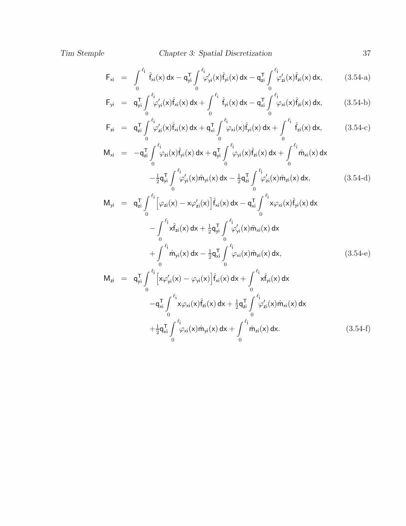
Tim Stemple Chapter 3: Spatial Discretization 37
∫ ∫ ∫` ` `i i iT ′ T ′ˆ ˆ ˆF = f (x) dx− q ϕ (x)f (x) dx− q ϕ (x)f (x) dx, (3.54-a)xi xi yi ziyi yi zi zi
0 0 0∫ ∫ ∫` ` `i i iT ′ Tˆ ˆ ˆF = q ϕ (x)f (x) dx + f (x) dx− q ϕ (x)f (x) dx, (3.54-b)yi xi yi xi ziyi yi xi
0 0 0∫ ∫ ∫` ` `i i iT ′ Tˆ ˆ ˆF = q ϕ (x)f (x) dx + q ϕ (x)f (x) dx + f (x) dx, (3.54-c)zi xi xi yi zizi zi xi
0 0 0∫ ∫ ∫` ` `i i iT Tˆ ˆ ˆM = −q ϕ (x)f (x) dx + q ϕ (x)f (x) dx + m (x) dxxi zi yi yi zi xizi yi
0 0 0∫ ∫` `i iT ′ T ′1 1ˆ ˆ− q ϕ (x)m (x) dx− q ϕ (x)m (x) dx, (3.54-d)yi ziyi yi zi zi2 2
0 0∫ ∫` `[ ]i iT ′ Tˆ ˆM = q ϕ (x)− xϕ (x) f (x) dx− q xϕ (x)f (x) dxyi zi xi xi yizi zi xi
0 0∫ ∫` `i iT ′1ˆ ˆ− xf (x) dx + q ϕ (x)m (x) dxzi xiyi yi2
0 0∫ ∫` `i iT1ˆ ˆ+ m (x) dx− q ϕ (x)m (x) dx, (3.54-e)yi xi zixi2
0 0∫ ∫` `[ ]i iT ′ ˆ ˆM = q xϕ (x)− ϕ (x) f (x) dx + xf (x) dxzi yi xi yiyi yi
0 0∫ ∫` `i iT T ′1ˆ ˆ−q xϕ (x)f (x) dx + q ϕ (x)m (x) dxxi zi xixi zi zi2
0 0∫ ∫` `i iT1+ q ϕ (x)m (x) dx + m (x) dx. (3.54-f)xi yi zixi2
0 0
Chapter 4 Equations of Motion
To each body i in the multibody system we associate another body j (Fig. 4), referred toas the body inboard to body i [20], and chosen so that the rigid body motion of body irelative to body j can be analyzed in an efficient manner. The inertial motion of each bodyin the structure can be determined recursively, by working backwards from the body, to itsinboard body, and then finally to the base body, referred to as body 1. Furthermore, thebody inboard to body 1 is taken to be the inertial space, referred to as body 0 (zero).
4.1 Generalized Coordinates
′ ′ ′ ′We introduce a coordinate system O ; x y z , which is fixed on body j (Fig. 4), and assumeii i i′ ′ ′ ′that the motion of coordinate system O ; x y z relative to coordinate system O ; x y z i ii i i i i i
depends just on generalized coordinates[ ]TNqri1 2q = , (4.1)q q · · · qri ri ri ri
and quasi-velocities [ ]TN1 2 wriw = , (4.2)w w · · · wri ri ri ri
in which N ≤ N . Recall from the meaning of quasi-velocity [32] that this implies thewri qri
existence of two N -by-N matrices A and B , both functions of q , which satisfy theqri wri ri ri ri
relations
q = B w , (4.3)ri ririTw = A q . (4.4)ri riri
38
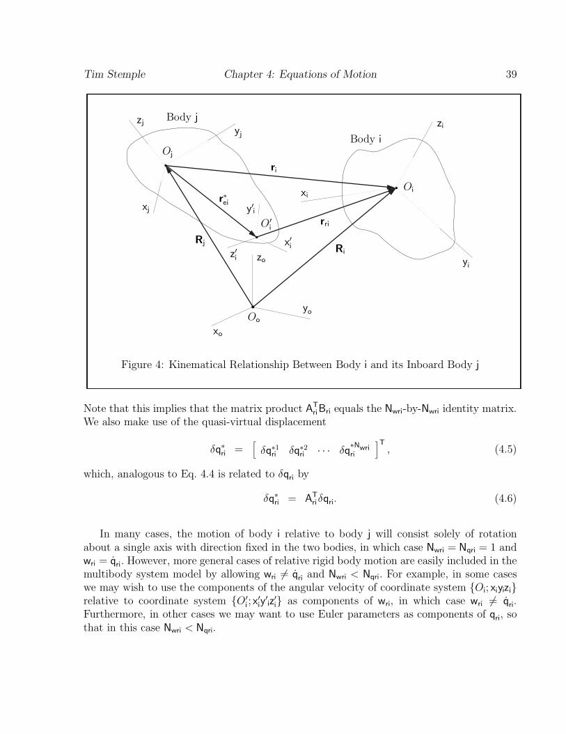
Tim Stemple Chapter 4: Equations of Motion 39
Body jzj ziyj
Body iOj
ri
Oixi∗rei ′xj y i
′ rriOi
′Rj xi R′ izi zo yi
yoOo
xo
Figure 4: Kinematical Relationship Between Body i and its Inboard Body j
TNote that this implies that the matrix product A B equals the N -by-N identity matrix.ri wri wriri
We also make use of the quasi-virtual displacement[ ]T∗N∗ ∗1 ∗2 wriδq = , (4.5)δq δq · · · δqri ri ri ri
which, analogous to Eq. 4.4 is related to δq byri
T∗δq = A δq . (4.6)riri ri
In many cases, the motion of body i relative to body j will consist solely of rotationabout a single axis with direction fixed in the two bodies, in which case N = N = 1 andwri qri
˙w = q . However, more general cases of relative rigid body motion are easily included in theri ri
˙multibody system model by allowing w 6= q and N < N . For example, in some casesri wri qriri
we may wish to use the components of the angular velocity of coordinate system O ; x yz ii i i′ ′ ′ ′relative to coordinate system O ; x y z as components of w , in which case w 6= q .i ri ri rii i i
Furthermore, in other cases we may want to use Euler parameters as components of q , sori
that in this case N < N .wri qri
Tim Stemple Chapter 4: Equations of Motion 40
We turn now to a consideration of the structure as a whole, and let[ ] [ ]T TNqr T T T1 2 q q · · · qq = = , (4.7)q q · · · qrr r1 r2 rNr r[ ] [ ]T T1 2 N T T Teq = q q · · · q = q q · · · q , (4.8)e e e e e1 e2 eN[ ] [ ]T T1 2 Nq T Tq = q q · · · q = q q , (4.9)r e[ ] [ ]T T1 2 N T T Twrw = w w · · · w = w w · · · w , (4.10)r r r r r1 r2 rN[ ] [ ]T TT1 2 N Twrw w · · · w ˙w = = w q , (4.11)r e[ ] [ ]T T∗ ∗1 ∗2 ∗N ∗T ∗T ∗Twrδq = δq δq · · · δq = δq δq · · · δq , (4.12)r r r r r1 r2 rN[ ] [ ]T T∗ ∗1 ∗2 ∗N ∗T Twδq = δq δq · · · δq = δq δq , (4.13)r e
j j j j j ∗j ∗jin which q , q , q , w , w , δq and δq are scalars, andr e r r
N = N + N + · · ·+ N , (4.14)qr qr1 qr2 qrN
N = N + N + · · ·+ N , (4.15)wr wr1 wr2 wrN
N = N + N + · · ·+ N , (4.16)e e1 e2 eN
N = N + N , (4.17)q qr e
N = N + N . (4.18)w wr e
Furthermore, we define the N -by-N matrixq w [ ]B = block-diag B , B , . . . , B , I , (4.19)r1 r2 rN
where in this case I equals the N -by-N identity matrix, and point out that Eq. 4.3 and thee e
definitions of q and w imply thatq = Bw. (4.20)
Finally, we let [ ]T∗N∗ ∗1 ∗2 wriT = (4.21)T T · · · Tri ri ri ri
∗jbe the generalized force associated with the quasi-velocity w , in which T is a scalar, andri ri
define [ ] [ ]T T∗ ∗1 ∗2 ∗N ∗T ∗T ∗TwrT = = , (4.22)T T · · · T T T · · · Tr r r r r1 r2 rN[ ] [ ]T T∗ ∗1 ∗2 ∗N ∗TwT = = , (4.23)T T · · · T T 0r
∗j ∗jin which 0 represents the N -by-1 zero matrix, and T and T are both scalars. Consequently,e r∗the virtual work performed by the generalized force T is given byri
∗∗TδW = δq T . (4.24)ri ri ri
Tim Stemple Chapter 4: Equations of Motion 41
4.2 Recursive Relations
˙ ˙˙In this section we develop the transformation from q, w and w to R , P , V , Ω , V and Ω ,i i i i i i
required in formulating the equations of motion. To begin with, r is the component matrixi−−→
of position vector r = O O (Fig. 4), C denotes the matrix of direction cosines of axes x yzii j i i i i
with respect to x y z and quasi-velocities v and ω are defined by the relationsjj j i i
˙v = C r , (4.25)i i i
T˙ω = C C , (4.26)i i i
with associated quasi-virtual displacements given by
∗δr = C δr , (4.27)i ii
∗ Tδθ = C δC . (4.28)i i i
(No confusion should arise from the fact that the symbols r and r used here have a differenti i
meaning than in Chapters 2 and 3.)
Based on the discussion of the preceding section, r and C depend only on q , q , andi i ej ri
possibly t. An application of the chain rule implies that
˙v = C r ,i i i( )∂r ∂r ∂ri i i˙ ˙= C q + q +i ri ejT∂q ∂q ∂tri ej( ) ( )∂r ∂r ∂ri i i
˙= C B w + C q + C , (4.29)i ri ri i iejT∂q ∂q ∂tri ej
where the last equality follows from Eq. 4.3; note, too, that a similar expression holds for˙ω . Next, if we were to continue in this manner and calculate v and ω , we would find thati i i
T T T˙the 6-by-1 matrix [v ω ] can be written in the formi i [ ]vi ˙ ¨= h w + h q − d , (4.30)ri r ei ieωi
with local quasi-virtual displacements satisfying the relation[ ]∗δr ∗i = h δq + h δq , (4.31)∗ ri eir eδθi
with h a 6-by-N matrix and h a 6-by-N matrix, with both dependent only on q andri wr ei e ri
t, and d is a 6-by-1 matrix which depends only on q , w and t. The derivation of specifici riri
formulas for h , h and d must be carried out case by case, depending on the type of jointri ei i
Tim Stemple Chapter 4: Equations of Motion 42
model involved, and is postponed to a later chapter. In a similar manner, since R and Pi i
are functions of q , q and t, we conclude thatr e [ ]Vi = H w + H q − D , (4.32)ri r ei ieΩi[ ]∗δR ∗i = H δq + H δq , (4.33)∗ ri ei erδΘi
where H is a 6-by-N matrix and H is 6-by-N , with both dependent only on q , q and t,ri wr ei e r e
˙and D is a 6-by-1 matrix which depends only on q , w , q , q and t.i rr e e
Recall now that the body inboard to body 1 is the inertial space (body 0), which impliesthat
R = r , (4.34)1 1
P = C , (4.35)1 1[ ] [ ]V v1 1= , (4.36)Ω ω1 1
H = h , (4.37)r1 r1
H = h , (4.38)e1 e1
D = d . (4.39)1 1
These equations initiate the recursion process described next.
With reference to Fig. 4, we see that the vector equation
R = R + r , (4.40)i j i
written in terms of component matrices, takes the form
TR = R + P r . (4.41)i j j i
Furthermore, based on the definitions of the matrices of direction cosines, P , P and C , wei j i
also have thatP = C P . (4.42)i i j
Now take derivatives with respect to time, yielding
˙V = P Ri i i( )T T˜˙ ˙= C P R + P Ω r + P ri j j j j i j i( )
˜= C V − r Ω + v , (4.43)i j i j i
T˜ ˙Ω = P Pi i i ( )T TT T˜ ˜= C P P Ω C + P C ωi j j j i j i i
T˜ ˜= C Ω C + ωi j i i( )˜ ˜= C Ω + ω ,i j i
Tim Stemple Chapter 4: Equations of Motion 43
which implies thatΩ = C Ω + ω . (4.44)i i j i
Combining Eqs. 4.43 and 4.44, we can write[ ] [ ] [ ]V V v∗i j i= B + , (4.45)iΩ Ω ωi j i
where [ ]˜C −C r∗ i i iB = . (4.46)i 0 Ci
Analogous to Eq 4.45 we also have that[ ] [ ] [ ]∗ ∗ ∗δRδR δr∗i j i= B + . (4.47)∗ i ∗ ∗δΘ δΘ δθi ij
Now take the time derivative of Eq. 4.45, to get that[ ] [ ] [ ] [ ]˙ ˙ ˙V V v V∗ ∗i j i j˙= B + + B , (4.48)i i˙ ˙ ω ΩΩ Ω i ji j
where, making use of Eqs. 4.43 and 4.44, we see that[ ] [ ] [ ]˜˜ ˜V V−ω C ω C r − C r∗ j ji i i i i i iB =i ˜Ω Ω0 −ω Cj ji i[ ]
˜˜−ω C V + ω C r Ω − C r Ωi i j i i i j i i j= ˜−ω C Ωi i j[ ]˜˜ ˜ ˜−ω (V + C r Ω − v ) + ω C r Ω − v C Ωi i i i j i i i i j i i j= ˜−ω (Ω − ω )i i i[ ]˜ ˜ ˜−ω V + ω v − v (Ω − ω )i i i i i i i= ˜−ωΩi i[ ] [ ]ω v Vi i i= − , (4.49)˜0 ω Ωi i
so that [ ] [ ] [ ] [ ]˙ ˙ ˙V V v V∗i j i i∗= B + − X , (4.50)i i˙ ˙ ω ΩΩ Ω i ii j
in which [ ]ω vi i∗X = . (4.51)i ˜0 ωi
Next, we develop recursive relations which can be used to compute H , H and D . Tori ei i
this end, combine Eqs. 4.30, 4.32 and 4.50 to get that
Tim Stemple Chapter 4: Equations of Motion 44[ ]Vi˙ ¨H w + H q − D =ri r ei ie Ωi[ ] [ ] [ ]
˙ ˙V v V∗ j i i∗= B + − Xi i˙ ω ΩΩ i ij [ ]V∗ i∗= B (H w + H q − D ) + (h w + h q − d )− Xi rj r ej j ri r ei ie e i Ωi( [ ])
V∗ ∗ ∗ i∗˙ ¨= (B H + h )w + (B H + h )q − B D + d + X . (4.52)i rj ri r i ej ei i j ie i Ωi
The obvious solution, and the one we use, is to take
∗H = B H + h , (4.53)ri i rj ri
∗H = B H + h , (4.54)ei i ej ei [ ]
V∗ i∗D = B D + d + X . (4.55)i i j i i Ωi
The recursive process is easily carried out by first requiring j < i (this places absolutely norestrictions on the structure). Then, use Eqs. 4.34, 4.35, 4.36, 4.37, 4.38 and 4.39 to computethe motion of body 1, and subsequently use Eqs. 4.41, 4.42, 4.45, 4.53, 4.54 and 4.55 tocompute the motion of bodies 2, 3, . . . , N, in that order.
4.3 Discretized Equations of Motion
At this point we have enough information to develop the final form of the discretized equa-tions of motion. To begin with, we note that the formula for R given in Eq. 2.38 for a rigidi
body has precisely the same form as the formula for R given in Eq. 3.50 for a second-orderi
Rayleigh beam, provided that for the rigid body case we set N = 0. In fact, this form of Rei i
is quite general, in that any other discretized beam model, or for that matter, any discretizedplate or shell model, would also result in the same form for R . Consequently, we can proceedi
by substituting Eq. 3.50 into Eq. 2.1, to get that ( [ ] )N [ ] ˙∑ Vi∗T∗T0 = M + M q − GδR δΘ rri rei rii eii Ωii=1 ( [ ] ) ∫N˙ ∑ViTT T ∗¨+ δq M + M q − G − δz τ dA. (4.56)eei eieiei rei i oiΩi i=1 ∂Boi
∗Recall that τ , which is the component matrix, along inertial axes x y z , of part of theoo ooi
surface traction, is nonzero only on that part of body i which contacts another body in thestructure. However, we include here the forces acting between the base (body 1) and the
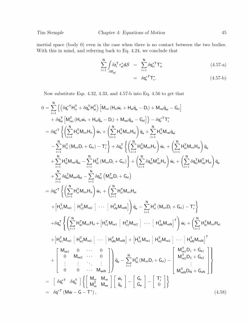
Tim Stemple Chapter 4: Equations of Motion 45
inertial space (body 0) even in the case when there is no contact between the two bodies.With this in mind, and referring back to Eq. 4.24, we conclude that
∫N N∑ ∑ ∗T ∗ ∗Tδz τ dS = δq T (4.57-a)i oi ri rii=1 i=1∂Boi
∗∗T= δq T . (4.57-b)r r
Now substitute Eqs. 4.32, 4.33, and 4.57-b into Eq. 4.56 to get that
N ( ) [ ]∑T T∗T T ˙ ¨ ¨0 = δq H + δq H M (H w + H q − D ) + M q − Grri ri r ei i rei rir ri e ei e ei
i=1 [ ]T ∗T ∗T˙ ¨ ¨+ δq M (H w + H q − D ) + M q − G − δq Tri r ei i eei eiei rei e ei r r( ) ( )
N N N∑ ∑ ∑T T T∗T ˙ ¨ ¨= δq H M H w + H M H q + H M qrri ri r rri ei reie eir ri ri ri
i=1 i=1 i=1 ( ) ( )N N N∑ ∑ ∑
T ∗ T T T˙ ¨− H (M D + G )− T + δq H M H w + H M H qrri i ri rri ri r rri eiri r e ei ei ei=1 i=1 i=1 ( ) ( )N N N N∑ ∑ ∑ ∑
T T T TT T+ H M q − H (M D + G ) + δq M H w + δq M H qrei rri i ri ri r eiei eei ei ei rei ei reii=1 i=1 i=1 i=1
N N ( )∑ ∑TT T¨+ δq M q − δq M D + Geei i eieiei ei rei
i=1 i=1( ) (N N∑ ∑∗T T T˙= δq H M H w + H M Hrri ri r rri eir ri ri
i=1 i=1 N[ . . . ] ∑. . .T T T T ∗. . . . . . ¨+ H M H M · · · H M q − H (M D + G )− Tre1 re2 reN rri i ri. . .r1 r2 rN e ri r. . .
i=1 (N N [ ]. . .∑ ∑T. . .T T T T TT . . . . . .+δq H M H + H M H M · · · H M w + H M Hrri ri re1 re2 reN r rri ei. . .e ei r1 r2 rN ei . . .
i=1 i=1[ . . . ] [ . . . ]T. . . . . .T T T T T T. . . . . .. . . . . .+ H M H M · · · H M + H M H M · · · H Mre1 re2 reN re1 re2 reN. . . . . .e1 e2 eN e1 e2 eN. . . . . . T M D + GM 0 · · · 0 1 e1re1ee1 TN ∑0 M · · · 0 M D + Gee2 2 e2 re2T ¨+ q − H (M D + G )− . . . rri i ri. e ei .. . . . .. . . . . i=1 T 0 0 · · · MeeN M D + GN eNreN[ ] [ ] [ ] [ ]∗[ ] M M w G Trr re r r∗T T r= δq δq − −Tr e q G 0M M eee ere
∗T ∗˙= δq (Mw− G− T ) , (4.58)
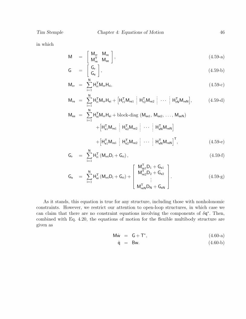
Tim Stemple Chapter 4: Equations of Motion 46
in which [ ]M Mrr reM = , (4.59-a)TM Meere[ ]GrG = , (4.59-b)Ge
N∑TM = H M H , (4.59-c)rr rr riri
i=1
N [ ]. . .∑ . . .T T T T. . .. . .M = H M H + H M H M · · · H M , (4.59-d)re rr ei re1 re2 reN. . .ri r1 r2 rN. . .i=1
N∑TM = H M H + block-diag (M , M , . . . , M )ee rr ei ee1 ee2 eeNei
i=1 [ ]. . .. . .T T T. . .. . .+ H M H M · · · H Mre1 re2 reN. . .e1 e2 eN. . .[ . . . ]T. . .T T T. . .. . .+ H M H M · · · H M , (4.59-e)re1 re2 reN. . .e1 e2 eN. . .N∑
TG = H (M D + G ) , (4.59-f)r rri i ririi=1 TM D + G1 e1re1 TN∑ M D + G 2 e2re2T G = H (M D + G ) + . (4.59-g)e rri i ri .ei . .i=1
TM D + GN eNreN
As it stands, this equation is true for any structure, including those with nonholonomicconstraints. However, we restrict our attention to open-loop structures, in which case we
∗can claim that there are no constraint equations involving the components of δq . Then,combined with Eq. 4.20, the equations of motion for the flexible multibody structure aregiven as
∗˙Mw = G + T , (4.60-a)
q = Bw. (4.60-b)
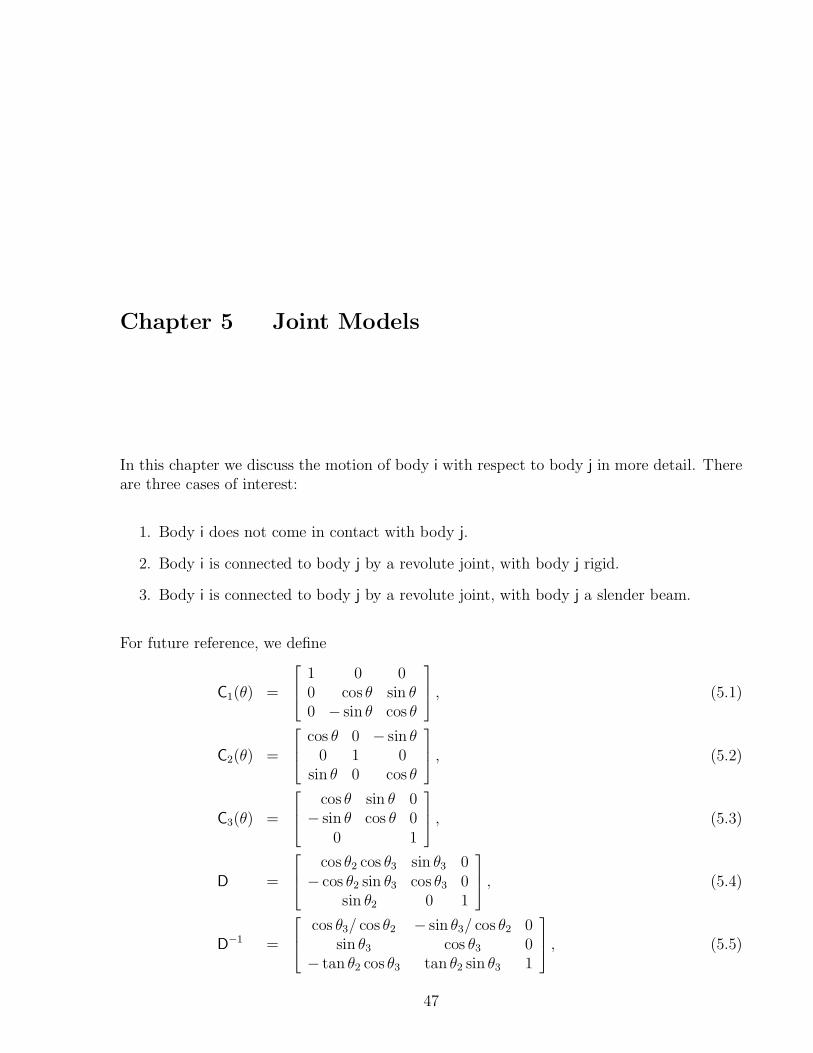
Chapter 5 Joint Models
In this chapter we discuss the motion of body i with respect to body j in more detail. Thereare three cases of interest:
1. Body i does not come in contact with body j.
2. Body i is connected to body j by a revolute joint, with body j rigid.
3. Body i is connected to body j by a revolute joint, with body j a slender beam.
For future reference, we define 1 0 0 C (θ) = 0 cos θ sin θ , (5.1) 1
0 − sin θ cos θ cos θ 0 − sin θ 0 1 0C (θ) = , (5.2) 2
sin θ 0 cos θ cos θ sin θ 0 − sin θ cos θ 0C (θ) = , (5.3) 3
0 1 cos θ cos θ sin θ 02 3 3 D = − cos θ sin θ cos θ 0 , (5.4) 2 3 3
sin θ 0 12 cos θ / cos θ − sin θ / cos θ 03 2 3 2 −1D = sin θ cos θ 0 , (5.5) 3 3
− tan θ cos θ tan θ sin θ 12 3 2 3
47
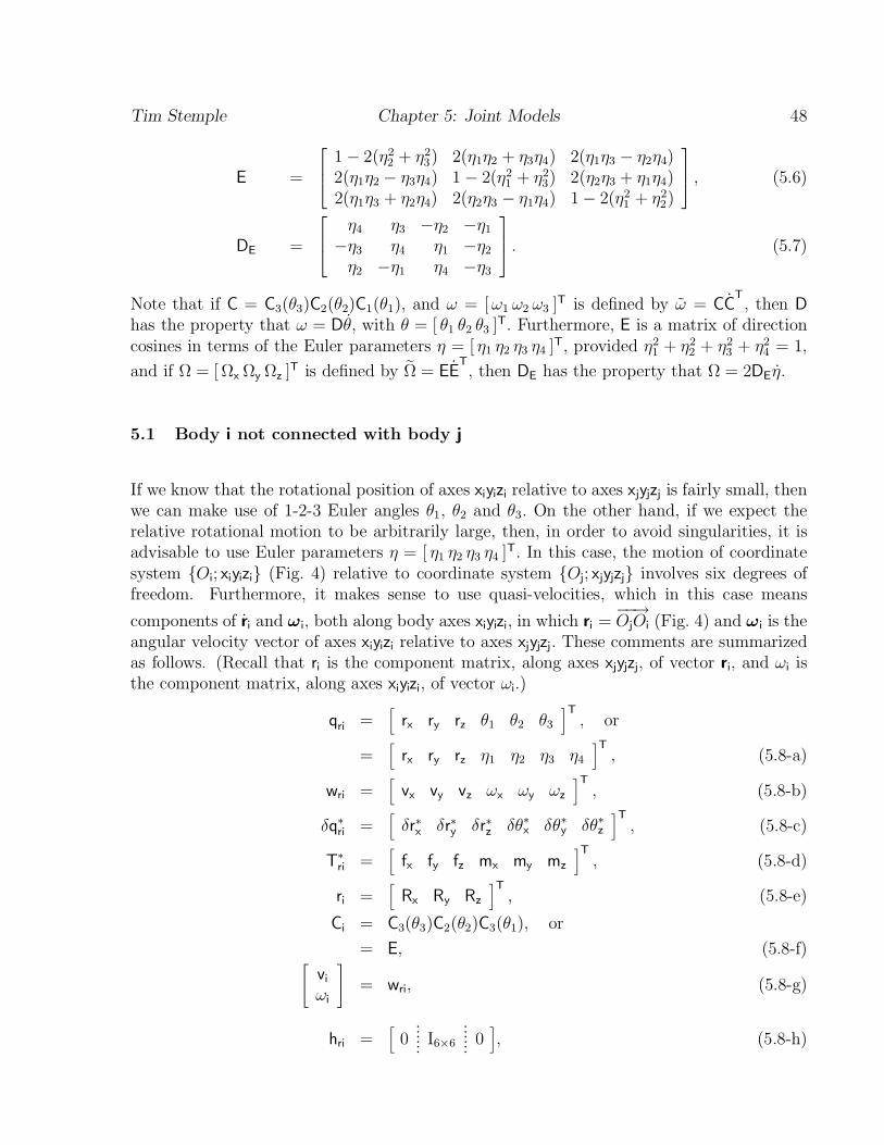
Tim Stemple Chapter 5: Joint Models 48
2 21− 2(η + η ) 2(η η + η η ) 2(η η − η η )1 2 3 4 1 3 2 42 3 2 2E = 2(η η − η η ) 1− 2(η + η ) 2(η η + η η ) , (5.6) 1 2 3 4 2 3 1 41 3
2 22(η η + η η ) 2(η η − η η ) 1− 2(η + η )1 3 2 4 2 3 1 4 1 2 η η −η −η4 3 2 1 D = −η η η −η . (5.7) E 3 4 1 2
η −η η −η2 1 4 3
TT ˙Note that if C = C (θ )C (θ )C (θ ), and ω = [ω ω ω ] is defined by ω = CC , then D3 3 2 2 1 1 1 2 3T˙has the property that ω = Dθ, with θ = [ θ θ θ ] . Furthermore, E is a matrix of direction1 2 3
T 2 2 2 2cosines in terms of the Euler parameters η = [ η η η η ] , provided η + η + η + η = 1,1 2 3 4 1 2 3 4TT ˜ ˙and if Ω = [ Ω Ω Ω ] is defined by Ω = EE , then D has the property that Ω = 2D η.x y z E E
5.1 Body i not connected with body j
If we know that the rotational position of axes x y z relative to axes x y z is fairly small, theni ji i j j
we can make use of 1-2-3 Euler angles θ , θ and θ . On the other hand, if we expect the1 2 3
relative rotational motion to be arbitrarily large, then, in order to avoid singularities, it isTadvisable to use Euler parameters η = [ η η η η ] . In this case, the motion of coordinate1 2 3 4
system O ; x y z (Fig. 4) relative to coordinate system O ; x y z involves six degrees ofi ji i i j j j
freedom. Furthermore, it makes sense to use quasi-velocities, which in this case means−−→
˙components of r and ω , both along body axes x y z , in which r = O O (Fig. 4) and ω is theii i i i i j i i
angular velocity vector of axes x y z relative to axes x y z . These comments are summarizedi ji i j j
as follows. (Recall that r is the component matrix, along axes x y z , of vector r , and ω isji j j i i
the component matrix, along axes x yz , of vector ω .)ii i i[ ]Tq = r r r θ θ θ , orx y z 1 2 3ri [ ]T
= r r r η η η η , (5.8-a)x y z 1 2 3 4[ ]Tv v v ω ω ωw = , (5.8-b)ri x y z x y z[ ]T∗ ∗ ∗∗ ∗ ∗ ∗δr δr δr δθ δθ δθδq = , (5.8-c)x y zx y zri [ ]T∗T = f f f m m m , (5.8-d)x y z x y zri [ ]T
r = R R R , (5.8-e)x y zi
C = C (θ )C (θ )C (θ ), ori 3 3 2 2 3 1
= E, (5.8-f)[ ]vi = w , (5.8-g)riωi [ . . ]. .. .. .h = 0 I 0 , (5.8-h)ri 6×6. .. .
Tim Stemple Chapter 5: Joint Models 49
h = 0, (5.8-i)ei
d = 0, (5.8-j)i [ ]TC 0iB = , orri −10 D[ ]TC 0i= . (5.8-k)T10 DE2
5.2 Body i connected to body j by a revolute joint
In this case, the motion of body i with respect to body j involves both the elastic motion ofbody j, as well as the rigid body motion of one body with respect to the other. We let rri−−→′′ ′ ′be the component matrix, along axes x y z of position vector r = O O and C the matrixi ri i rii i i
′ ′ ′ ∗of direction cosines of axes x y z with respect to axes x y z (Fig. 4). Likewise, r is thei ii i i i ei−−→ ∗′∗component matrix, along axes x y z of vector r = OO , and C is the matrix of directionjj j jei i ei′ ′ ′cosines of axes x y z with respect to axes x y z . These definitions imply thati jj ji i
∗T∗r = r + C r , (5.9)i riei ei∗C = C C . (5.10)i ri ei
We also let ω be the component matrix, along axes x yz , of the angular velocity vector ofiri i i∗′ ′ ′axes x yz with respect to axes x y z and δθ the associated quasi-virtual displacement, soi ii i rii i
that
T˙ω = C C , (5.11)ri ri ri
∗ TδΘ = C δC , (5.12)ri ri ri
and let the 3-by-N matrix h and 3-by-1 matrix d satisfy the relationswr ωri ωri
˙ω = h w − d , (5.13)ri ωri r ωri
∗ ∗δθ = h δq . (5.14)ri ωri r
′For revolute joints, point O on body j, and point O on body i occupy the same location inii∗space, and consequently, r = 0 and r = r .ri i ei
There are several choices available for q and w , depending on the number of rotationalriri
degrees of freedom at the joint. We display next those cases of immediate interest. Theparticular example we consider in the next chapter has joints with one, two or three rotationaldegrees of freedom. Furthermore, each degree of freedom is directly controlled by a separate
∗actuator, in the sense that if θ is the rotational degree of freedom and T is the torque effected∗by the actuator, then T δθ is the associated virtual work. We can actually cover all pertinent
cases simultaneously by considereing a joint with three degrees of rotational freedom. To be
Tim Stemple Chapter 5: Joint Models 50
precise, there are three rotations in series, with the first a 1-rotation, the second a 2-rotationand the third a 3-rotation. Equations which correspond to joints with one or two degrees offreedom can be obtained by setting two, or one, of the angles to zero. Letting θ , θ and θ1 2 3
be the rotational degrees of freedom and M , M and M the corresponding control torques,1 2 3
the pertinent equations take the form
[ ]Tθ θ θq = , (5.15-a)1 2 3ri [ ]T˙ ˙ ˙ ˙w = = q , (5.15-b)θ θ θri 1 2 3 ri[ ]T∗δq = δθ δθ δθ = δq , (5.15-c)1 2 2 riri [ ]T∗T = M M M , (5.15-d)1 2 3ri
C = C (θ )C (θ )C (θ ), (5.15-e)ri 3 3 2 2 1 1
ω = Dw , (5.15-f)ri ri[ ]. .. .. .. .h = 0 D 0 , (5.15-g)ωri . .. . sin θ cos θ cos θ sin θ − cos θ2 3 2 3 3 ˙ ˙ ˙ ˙ ˙ ˙d = θ θ − sin θ sin θ + θ θ cos θ cos θ + θ θ sin θ , (5.15-h) 2 3 2 3 3ωri 1 2 1 3 2 3
− cos θ 0 02
A = I , (5.15-i)ri 3×3
B = I . (5.15-j)ri 3×3
5.2.1 Body j rigid
∗ T∗ ˙˜In this case, since body j is rigid, r and C are both constant, so that ω = C C =i i iei ei∗ ∗T T˜ ˜C C (C C ω ) = ω . Consequently,ri ri ri riei ei
∗ ∗r = r , (r a constant) (5.16)i ei ei∗ ∗C = C C , (C a constant) (5.17)i ri ei ei[ ] [ ]
v 0i = , (5.18)ω ωi ri[ ]
0h = , (5.19)ri hωri
h = 0, (5.20)ei [ ]0
d = . (5.21)i dωri
Tim Stemple Chapter 5: Joint Models 51
5.2.2 Body j a slender beam
′ ∗In this case, points O , O and O | (Figs. 2 and 4) coincide, so that r = r (` ) andi cj cj ji eix=`j∗C = E (` ). Referring to Eqs. 3.3, 5.9 and 5.10, we see thatcj jei
r = r (` ) = ` e + u (` ), (5.22)i cj j j 1 cj j
C = C E (` ). (5.23)i ri cj j
(To simplify matters, we drop the “(` )” for most of the following derivations.) Consequently,j
˙v = C ri i i
= C E u , (5.24)ri cj cj
T˙ω = C Ci i i [ ]˜T TT T˙ ˜= C E E (D ψ )C + E C ωri cj cj cj ri ri ricj cj( )˙= Tilde C D ψ + ω , (5.25)ri cj cj ri
where we have used Eqs. 3.7 and 5.23, so that
˙ω = C D ψ + ω . (5.26)i ri cj cj ri
Next, computing time derivatives of Eqs. 5.24 and 5.26 results in
˜˜v = C E u − ω v − C (D ψ )E ui ri cj cj ri i ri cj cj cj cj( )˙˜¨ ˙= C E u − ω v − Tilde C D ψ C E uri cj cj ri i ri cj cj ri cj cj˜ ˜ ˜= C E u − ω v − (ω − ω )vri cj cj ri i i ri i˜¨= C E u − ω v , (5.27)ri cj cj i i
¨ ˙ ˙˜ω = C D ψ + ω − ω (ω − ω ) + C D ψi ri cj cj ri ri i ri ri cj cj
¨ ˙ ˙˜= C D ψ + h w − (d + ω ω − C D ψ ). (5.28)ri cj cj ωri r ωri ri i ri cj cj
Combining Eqs. 5.24 and 5.26, and then Eqs. 5.27 and 5.28, we can write[ ] [ ] [ ] [ ]˙E uv C 0 0cj cji ri= + , (5.29)˙ω 0 C ωD ψi ri ricj cj[ ] [ ] [ ] [ ] [ ]˜¨E u ω vv C 0 0cj cj i ii ri= + w − . (5.30)r¨ ˙ ˙˜ω 0 C hD ψ d + ω ω − C D ψi ri ωricj cj ωri ri i ri cj cj
∗Regardless of the discretization method in use, we can identify a 6-by-N matrix Φ and ae j∗6-by-1 matrix d , so thatej [ ]
E ucj cj ∗ ˙= Φ q , (5.31)j e˙D ψcj cj[ ]¨E ucj cj ∗∗¨= Φ q − d . (5.32)j e ej¨D ψcj cj
Tim Stemple Chapter 5: Joint Models 52
Combining the previous four equations, and comparing the result with Eq. 4.30, we concludethat [ ] [ ] [ ]
v C 0 0i ri ∗ ˙= Φ q + , (5.33)j ejω 0 C ωi ri ri[ ]0
h = , (5.34)ri hωri[ ]C 0ri ∗h = Φ , (5.35)ei j0 Cri[ ] [ ]
ω v C 0i i ri ∗d = + d . (5.36)i ej˙ ˙˜ 0 Cd + ω ω − C D ψ riωri ri i ri cj cj
∗∗At this point we derive specific formulas for u (` ), E (` ), Φ and d , for the dis-cj j cj j j ej
cretized, second-order Rayleigh beam. Making use of Eqs. 3.37-a, 3.45-a, 3.45-b, 3.45-c,3.52-n and 3.52-o we see that ∫ ` [ ]j
T ′ ′T T ′ ′T1u (` ) = − q ϕ (s)ϕ (s)q + q ϕ (s)ϕ (s)q dsxj j yj zjyj yj yj zj zj zj2
0( )T T1 ¯ ¯′ ′ ′ ′= − q M q + q M q , (5.37)y y j z z jyj zjyj zj2
so that 1 T T¯ ¯′ ′ ′ ′− (q M q + q M q )y y j z z jyj yj zj zj2 T u (` ) = ϕ (` )q , (5.38)jcj j yjyj Tϕ (` )qj zjzj T T¯ ¯′ ′ ′ ′˙ ˙−q M q − q M qy y j z z jyj yj zj zj
T ˙u (` ) = ϕ (` )q , (5.39)jcj j yjyj Tϕ (` )qj zjzj TT T T¯ ¯ ¯ ¯′ ′ ′ ′ ′ ′ ′ ′¨ ¨ ˙ ˙ ˙−q M q − q M q − q M q − q M qy y j z z j y y j z z jyj zj yj zjyj zj yj zj
T u (` ) = ϕ (` )q . (5.40)cj j j yjyj T ¨ϕ (` )qjzj zj
Likewise, referring to Eqs. 3.37-b and 3.37-c, we see that Tϕ (` )qj xjxj 1′T T ′T −ϕ (` )q + q ϕ (` )ϕ (` )qψ (` ) = , (5.41)j xj j jcj j zj yjzj xj yj 21′T T ′Tϕ (` )q + q ϕ (` )ϕ (` )qj xj j jyj yj xj zj zj2 T ˙ϕ (` )qj xjxj 1 1′T T ′T T ′ T˙ −ϕ (` )q + q ϕ (` )ϕ (` )q + q ϕ (` )ϕ (` )qψ (` ) = , (5.42)j xj j j j jcj j zj yj xjzj xj yj yj yj xj 2 21 1′T T ′T T ′ T˙ ˙ ˙ϕ (` )q + q ϕ (` )ϕ (` )q + q ϕ (` )ϕ (` )qj xj j j j jyj yj xj zj zj zj zj xj xj2 2
Tim Stemple Chapter 5: Joint Models 53
T ¨ϕ (` )qj xjxj T1 1 1′T T ′T T ′ T ′¨ ¨ ¨ ¨ ˙ ˙−ϕ (` )q + q ϕ (` )ϕ (` )q + q ϕ (` )ϕ (` )q + q ϕ (` )ϕ (` )qψ (` ) = .j xj j j j j xj j jcj j zj zj xj yj yj yj yj xj xj xj yj yj 2 2 2T1 1 1′T T ′T T ′ T ′ϕ (` )q + q ϕ (` )ϕ (` )q + q ϕ (` )ϕ (` )q + q ϕ (` )ϕ (` )qj xj j j j j xj j jyj zj xj zjyj xj zj zj zj xj xj zj2 2 2
(5.43)
˙ ˙˙ ¨Now, referring to Eqs. 3.38-a and 3.38-b, we compute E u , E u , D ψ and E ψ , andcj cj cj cj cj cj cj cj
then compare the results with Eqs. 5.31 and 5.32 to obtain T ′ T T ′ T¯ ¯′ ′ ′ ′0 · · · 0 q (ϕ ϕ −M ) q (ϕ ϕ −M )y y j z z jyj yj yj zj zj zj T T T0 · · · 0 ϕ q ϕ ϕ xjyj xj zj T T T0 · · · 0 −q ϕ ϕ ϕ xjxj yj zj∗ Φ = , (5.44-a)j 1 1T T ′ ′T T ′ ′T ϕ q ϕ ϕ − q ϕ ϕ xj zj zj yj yj yj zj2 2 T ′T ′T 0 · · · 0 q ϕ ϕ −ϕxjxj yj zj
′T T ′T0 · · · 0 ϕ q ϕ ϕxjyj xj zj TT ¯ ¯′ ′ ′ ′q M q + q M qy y j z z jyj zjyj zj 0 0 ∗ d = . (5.44-b)ej 0 T ′T ˙ ˙q ϕ ϕ qxjxj yj yj
T ′Tq ϕ ϕ qxj zjxj zj
Finally, we note that the required formula for E is obtained by substituting Eqs. 3.45-a,cj
3.45-b and 3.45-c into Eq. 3.38-a.
Chapter 6 Numerical Example
The equations developed in this paper were used to create a general purpose computerprogram which was applied to a robot consisting of two flexible links — bodies 1 and 2 —with a rigid end effector — body 3 — as shown in Fig. 5. To simplify the mathematicalmodel somewhat, we assume that the joints have no mass and are dimensionless, whichimplies that the three axes of joint 1 intersect in a common point and that the three axes ofjoint 3 intersect in a common point. We have also assumed that the robot base is fixed inthe inertial space. Although this is certainly not the case for a space-based robot, keep inmind that for the space shuttle for example, the ratio of robot arm mass to shuttle mass isapproximately .0035, so that for the duration of the maneuvers we consider here (30 s), themotion of the base should have a minimal effect.
6.1 Shape Functions
In order to determine an appropriate choice of shape functions we first note that, relativeto coordinate system O ; x yz (Fig. 2), beam i should behave similar to a cantilever beamii i i
with a mass attached at the far end, where x = ` , i = 1, 2. This dictates that the geometrici
boundary conditions are given by
′ ′u (0) = u (0) = ψ (0) = u (0) = u (0) = 0. (6.1)yi zi xi yi zi
The dynamic boundary conditions are not time-invariant, as would be the case if coordinatesystem O ; x yz was fixed in the inertial space and there was simply a rigid-body fixed onii i i
the far end of the beam. Specific, albeit extremely complicated, expressions for the dynamicboundary conditions could be obtained from substituting Eq. 3.44, for i = 1, 2, and Eq. 2.38,
∗T ∗T Tfor i = 3, into Eq. 2.1. The equations are complicated by the fact that [δR δΘ ] involves22∗T∗T′ ′ Tδu (` ), δu (` ), δψ (` ), δu (` ) and δu (` ), and [δR δΘ ] involves δu (` ), δu (` ),y1 1 z1 1 x1 1 1 1 3 yi i zi iy1 z1 3
54
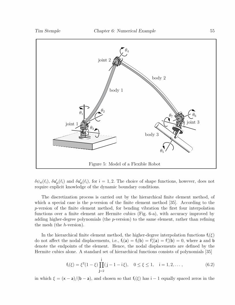
Tim Stemple Chapter 6: Numerical Example 55
θ4
joint 2
body 2
body 1
θ2θ1 θ6θ7
joint 3joint 1θ3
body 3
θ5
Figure 5: Model of a Flexible Robot
′ ′δψ (` ), δu (` ) and δu (` ), for i = 1, 2. The choice of shape functions, however, does notxi i i iyi zi
require explicit knowledge of the dynamic boundary conditions.
The discretization process is carried out by the hierarchical finite element method, ofwhich a special case is the p-version of the finite element method [35]. According to thep-version of the finite element method, for bending vibration the first four interpolationfunctions over a finite element are Hermite cubics (Fig. 6-a), with accuracy improved byadding higher-degree polynomials (the p-version) to the same element, rather than refiningthe mesh (the h-version).
In the hierarchical finite element method, the higher-degree interpolation functions f (ξ)i′ ′do not affect the nodal displacements, i.e., f (a) = f (b) = f (a) = f (b) = 0, where a and bi i i i
denote the endpoints of the element. Hence, the nodal displacements are defined by theHermite cubics alone. A standard set of hierarchical functions consists of polynomials [35]
i∏2f (ξ) = ξ (1− ξ) ( j− 1− i ξ), 0 ≤ ξ ≤ 1, i = 1, 2, . . . , (6.2)i
j=2
in which ξ = (x − a)/(b − a), and chosen so that f (ξ) has i− 1 equally spaced zeros in thei
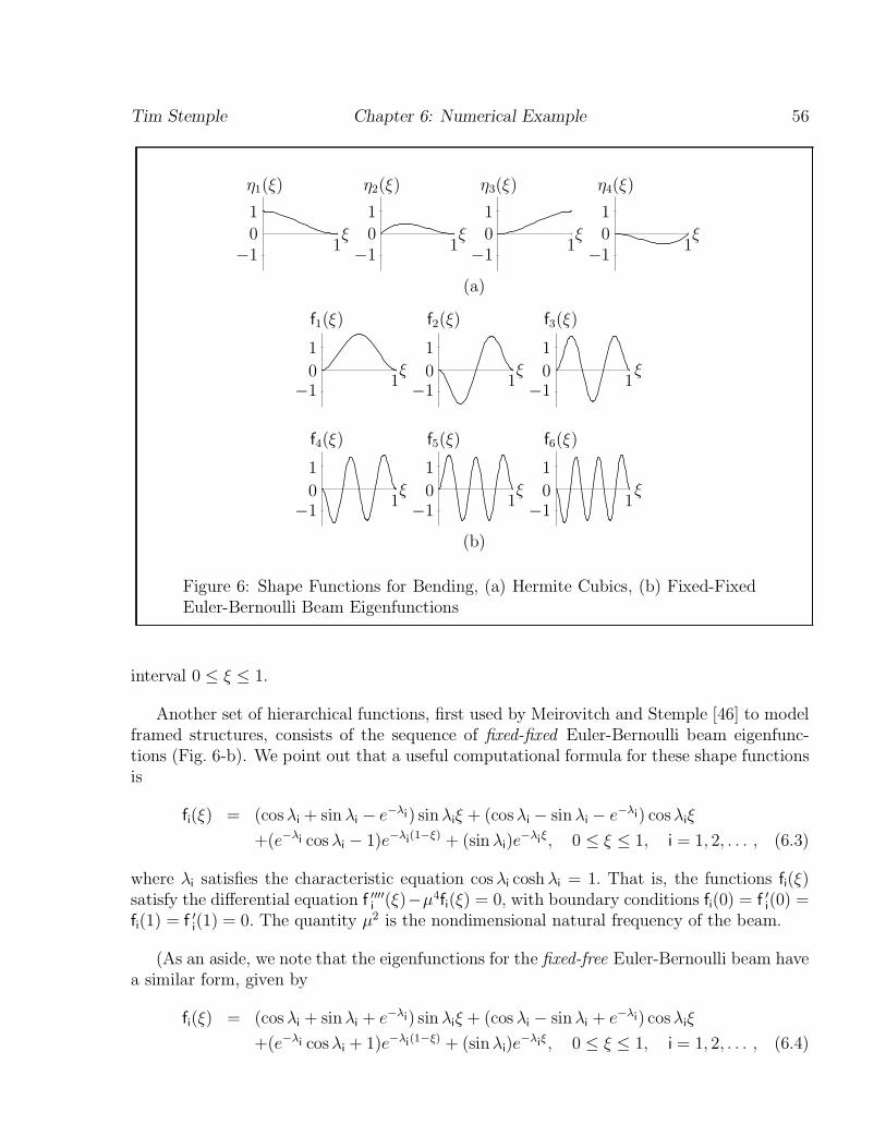
Tim Stemple Chapter 6: Numerical Example 56
η (ξ) η (ξ) η (ξ) η (ξ)1 2 3 4
1 1 1 1
0 ξ 0 ξ 0 ξ 0 ξ1 1 1 1−1 −1 −1 −1
(a)
f (ξ) f (ξ) f (ξ)1 2 3
1 1 1ξ ξ ξ0 0 0
1 1 1−1 −1 −1
f (ξ) f (ξ) f (ξ)4 5 6
1 1 1
ξ ξ ξ0 0 01 1 1−1 −1 −1
(b)
Figure 6: Shape Functions for Bending, (a) Hermite Cubics, (b) Fixed-FixedEuler-Bernoulli Beam Eigenfunctions
interval 0 ≤ ξ ≤ 1.
Another set of hierarchical functions, first used by Meirovitch and Stemple [46] to modelframed structures, consists of the sequence of fixed-fixed Euler-Bernoulli beam eigenfunc-tions (Fig. 6-b). We point out that a useful computational formula for these shape functionsis
−λ −λi if (ξ) = (cosλ + sin λ − e ) sinλ ξ + (cosλ − sinλ − e ) cosλ ξi i i i i i i
−λ −λ (1−ξ) −λ ξi i i+(e cos λ − 1)e + (sin λ )e , 0 ≤ ξ ≤ 1, i = 1, 2, . . . , (6.3)i i
where λ satisfies the characteristic equation cosλ cosh λ = 1. That is, the functions f (ξ)i i i i′′′′ 4 ′satisfy the differential equation f (ξ)−µ f (ξ) = 0, with boundary conditions f (0) = f (0) =i ii i
′ 2f (1) = f (1) = 0. The quantity µ is the nondimensional natural frequency of the beam.i i
(As an aside, we note that the eigenfunctions for the fixed-free Euler-Bernoulli beam havea similar form, given by
−λ −λi if (ξ) = (cos λ + sinλ + e ) sin λ ξ + (cos λ − sinλ + e ) cosλ ξi i i i i i i
−λ −λ (1−ξ) −λ ξi i i+(e cosλ + 1)e + (sinλ )e , 0 ≤ ξ ≤ 1, i = 1, 2, . . . , (6.4)i i
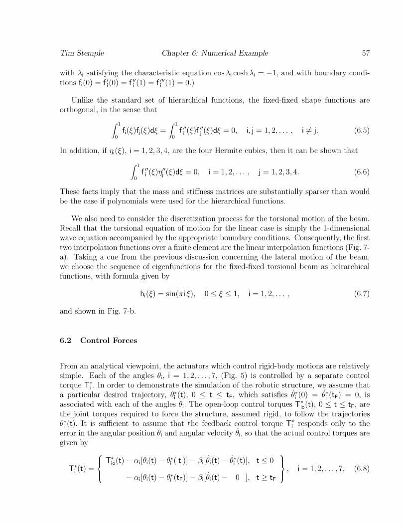
Tim Stemple Chapter 6: Numerical Example 57
with λ satisfying the characteristic equation cosλ coshλ = −1, and with boundary condi-i i i′ ′′ ′′′tions f (0) = f (0) = f (1) = f (1) = 0.)i i i i
Unlike the standard set of hierarchical functions, the fixed-fixed shape functions areorthogonal, in the sense that∫ ∫1 1
′′ ′′f (ξ)f (ξ)dξ = f (ξ)f (ξ)dξ = 0, i, j = 1, 2, . . . , i 6= j. (6.5)i j i j0 0
In addition, if η (ξ), i = 1, 2, 3, 4, are the four Hermite cubics, then it can be shown thati ∫ 1′′ ′′f (ξ)η (ξ)dξ = 0, i = 1, 2, . . . , j = 1, 2, 3, 4. (6.6)i j
0
These facts imply that the mass and stiffness matrices are substantially sparser than wouldbe the case if polynomials were used for the hierarchical functions.
We also need to consider the discretization process for the torsional motion of the beam.Recall that the torsional equation of motion for the linear case is simply the 1-dimensionalwave equation accompanied by the appropriate boundary conditions. Consequently, the firsttwo interpolation functions over a finite element are the linear interpolation functions (Fig. 7-a). Taking a cue from the previous discussion concerning the lateral motion of the beam,we choose the sequence of eigenfunctions for the fixed-fixed torsional beam as heirarchicalfunctions, with formula given by
h (ξ) = sin(πi ξ), 0 ≤ ξ ≤ 1, i = 1, 2, . . . , (6.7)i
and shown in Fig. 7-b.
6.2 Control Forces
From an analytical viewpoint, the actuators which control rigid-body motions are relativelysimple. Each of the angles θ , i = 1, 2, . . . , 7, (Fig. 5) is controlled by a separate controli
∗torque T . In order to demonstrate the simulation of the robotic structure, we assume thati∗ ∗ ∗˙ ˙a particular desired trajectory, θ (t), 0 ≤ t ≤ t , which satisfies θ (0) = θ (t ) = 0, isF Fi i i
∗associated with each of the angles θ . The open-loop control torques T (t), 0 ≤ t ≤ t , arei Fio
the joint torques required to force the structure, assumed rigid, to follow the trajectories∗∗θ (t). It is sufficient to assume that the feedback control torque T responds only to thei i
˙error in the angular position θ and angular velocity θ , so that the actual control torques arei i
given by ∗ ∗ ∗˙ ˙ T (t)− α [θ (t)− θ ( t )]− β [θ (t)− θ (t)], t ≤ 0 i i i iio i i∗T (t) = , i = 1, 2, . . . , 7, (6.8)i ∗ ˙− α [θ (t)− θ (t )]− β [θ (t)− 0 ], t ≥ ti i F i i Fi
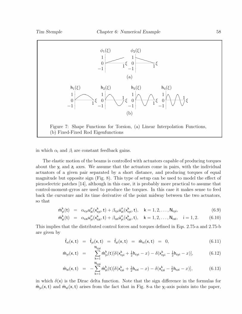
Tim Stemple Chapter 6: Numerical Example 58
φ (ξ) φ (ξ)1 2
1 1ξ ξ0 0
1 1−1 −1
(a)
h (ξ) h (ξ) h (ξ) h (ξ)1 2 3 4
1 1 1 11 1
ξ ξ ξ ξ0 0 0 01 1−1 −1 −1 −1
(b)
Figure 7: Shape Functions for Torsion, (a) Linear Interpolation Functions,(b) Fixed-Fixed Rod Eigenfunctions
in which α and β are constant feedback gains.i i
The elastic motion of the beams is controlled with actuators capable of producing torquesabout the y and z axes. We assume that the actuators come in pairs, with the individualii
actuators of a given pair separated by a short distance, and producing torques of equalmagnitude but opposite sign (Fig. 8). This type of setup can be used to model the effect ofpiezoelectric patches [14], although in this case, it is probably more practical to assume thatcontrol-moment-gyros are used to produce the torques. In this case it makes sense to feedback the curvature and its time derivative of the point midway between the two actuators,so that
k ′′ k ′′ kˆ ˙m (t) = α u (x , t) + β u (x , t), k = 1, 2, . . . ,N , (6.9)cyi cyi cyiyi zi cyi zi cyi
k ′′ k ′′ km (t) = α u (x , t) + β u (x , t), k = 1, 2, . . . ,N , i = 1, 2. (6.10)czi czi czizi yi czi yi czi
This implies that the distributed control forces and torques defined in Eqs. 2.75-a and 2.75-bare given by
ˆ ˆ ˆ ˆf (x, t) = f (x, t) = f (x, t) = m (x, t) = 0, (6.11)xi yi zi xi
Ncyi∑k k k1 1m (x, t) = m (t)[δ(x + h − x)− δ(x − h − x)], (6.12)yi cyi cyiyi cyi cyi2 2
k=1
Nczi∑k k k1 1ˆ ˆm (x, t) = − m (t)[δ(x + h − x)− δ(x − h − x)], (6.13)zi czi czizi czi czi2 2
k=1
in which δ(x) is the Dirac delta function. Note that the sign difference in the formulas forˆ ˆm (x, t) and m (x, t) arises from the fact that in Fig. 8-a the y -axis points into the paper,yi zi i
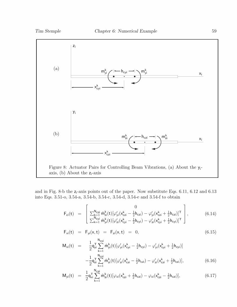
Tim Stemple Chapter 6: Numerical Example 59
zi
(a) k khm mcyiyi yi xi
kxcyi
yi
(b) k khm mczizi zi xi
kxczi
Figure 8: Actuator Pairs for Controlling Beam Vibrations, (a) About the y -iaxis, (b) About the z -axisi
and in Fig. 8-b the z -axis points out of the paper. Now substitute Eqs. 6.11, 6.12 and 6.13i
into Eqs. 3.51-o, 3.54-a, 3.54-b, 3.54-c, 3.54-d, 3.54-e and 3.54-f to obtain 0 ∑ N k 1 1′ k ′ k Tczi m (t)[ϕ (x − h )− ϕ (x + h )]F (t) = , (6.14)czi czici zi yi czi yi czik=1 2 2
N∑ cyi k 1 1′ k ′ k Tm (t)[ϕ (x − h )− ϕ (x + h )]cyi cyik=1 yi zi cyi zi cyi2 2
F (t) = F (x, t) = F (x, t) = 0, (6.15)xi yi zi
Ncyi∑1 kT ′ k ′ k1 1ˆM (t) = q m (t)[ϕ (x − h )− ϕ (x + h )]xi cyi cyiyi yi yi cyi yi cyi2 22k=1
Nczi∑1 kT ′ k ′ k1 1− q m (t)[ϕ (x − h )− ϕ (x + h )], (6.16)czi czizi zi zi czi zi czi2 22 k=1
Nczi∑1 kT k k1 1ˆM (t) = q m (t)[ϕ (x + h )− ϕ (x − h )], (6.17)yi xi czi xi czixi zi czi czi2 22 k=1
Tim Stemple Chapter 6: Numerical Example 60
Ncyi∑1 kT k k1 1ˆM (t) = q m (t)[ϕ (x + h )− ϕ (x − h )]. (6.18)zi xi cyi xi cyixi yi cyi cyi2 22k=1
6.3 Simulation Results
As mentioned earlier, we consider a flexible space robot comprised of two slender beams anda rigid end-effector (Fig. 5). Furthermore, the first and third joints have three degrees offreedom, with the motion described by a 1-rotation, 2-rotation, and 3-rotation, in series,and the second joint, which has one degree of freedom, is described by a 2-rotation, so thatN = N = 7. The system parameters for the structure are given as follows:qr wr
` = 4 m, ρ = 21.6 kg/m, i = 1, 2,i ci
−6 4 −6 4ˆ ˆ ˆI = 9.84× 10 m , I = I = 4.92× 10 m , i = 1, 2,xxi yyi zzi
2m = 62.1 kg, J = diag[ 35.6, 85.4, 115.0 ] kg-m .3 e3
For the particular numerical example under consideration, we use only one finite elementper beam, with six hierarchical functions for lateral motion, and four hierarchical functionsfor torsional motion. Due to the nature of the the geometric boundary conditions, Eq. 6.1,the first two Hermite cubics η (ξ) and η (ξ) (Fig. 6-a), and the first linear interpolation1 2
function φ (ξ) (Fig. 7-a), are not required. Consequently, N = 5 and N = N = 8, for1 xi yi zi
i = 1, 2. Considering also that the first and third joints have three degrees of freedom, and thesecond joint one degree of freedom, we conclude that the structural model has N = N = 49q w
degrees of freedom.
The feedback gains for joint control were chosen to be
α = 1000, β = 2000, i = 1, 2, . . . , 7, (6.19)i i
with four actuator pairs on each of the two beams to control the elastic motion. That is,1 1 2 2N = N = 2, with locations x = x = .15 m, x = x = 3.75 m, separation distancescyi czi cyi czi cyi czi
h = h = .1 m, i = 1, 2 and feedback gains given bycyi czi
k k k kα = α = 15, 000, β = β = 22, 500, k = 1, 2, 3, 4, i = 1, 2. (6.20)cyi czi cyi czi
The desired joint angle trajectories were chosen to be[ ( )]θ 2πt 2πtFi∗θ (t) = − sin , 0 ≤ t ≤ t , (6.21)Fi 2π t tF F
∗ ∗ ∗in which θ = θ (t ). Note that this function satisfies the conditions θ (0) = 0, θ (t ) = θ ,Fi F F Fii i i∗ ∗ ∗ ∗˙ ¨ ˙ ¨and is rather smooth, in the sense that θ (0) = θ (0) = θ (t ) = θ (t ) = 0. The totalF Fi i i i
simulation time was 30 s, with t = 20 s andF
θ = −1 rad, θ = −.5 rad, θ = .5 rad, θ = 1.5 rad,F1 F2 F3 F4 (6.22)θ = 1.25 rad, θ = .5 rad, θ = −.75 rad.F5 F6 F7
Tim Stemple Chapter 6: Numerical Example 61
∗Plots of the functions θ (t) are shown with open circles in Fig. 9.i
The system of ordinary differential equations, Eqs. 4.60-a and 4.60-b, were integratedusing the IMSL subroutine DIVPAG, which uses the BDF method, also known as Gear’sstiff method, with the results plotted in Figs. 9, 10, 11 and 12. Three different simulationswere performed. In the first case, the structure is assumed to be rigid, with all feedbackgains set to zero. The resulting angular and flexible displacements are simply the desiredtrajectories, and are shown with open circles. In the second case, the flexibility of the beamsis included, but with all of the feedback gains still equal to zero. These results are shownwith a dotted line. And finally, in the third case, the feedback gains are as indicated earlier,with the results shown with a solid line. Figure 9 shows time histories of the joint angles,Fig. 10 shows time histories of the beam tip angular, axial and lateral displacements, ψ (` ),xi i
u (` ), u (` ) and u (` ), i = 1, 2, the joint control torques are shown in Fig. 11, and thexi i yi i zi i
actuator pair control torque time histories are shown in Fig. 12.
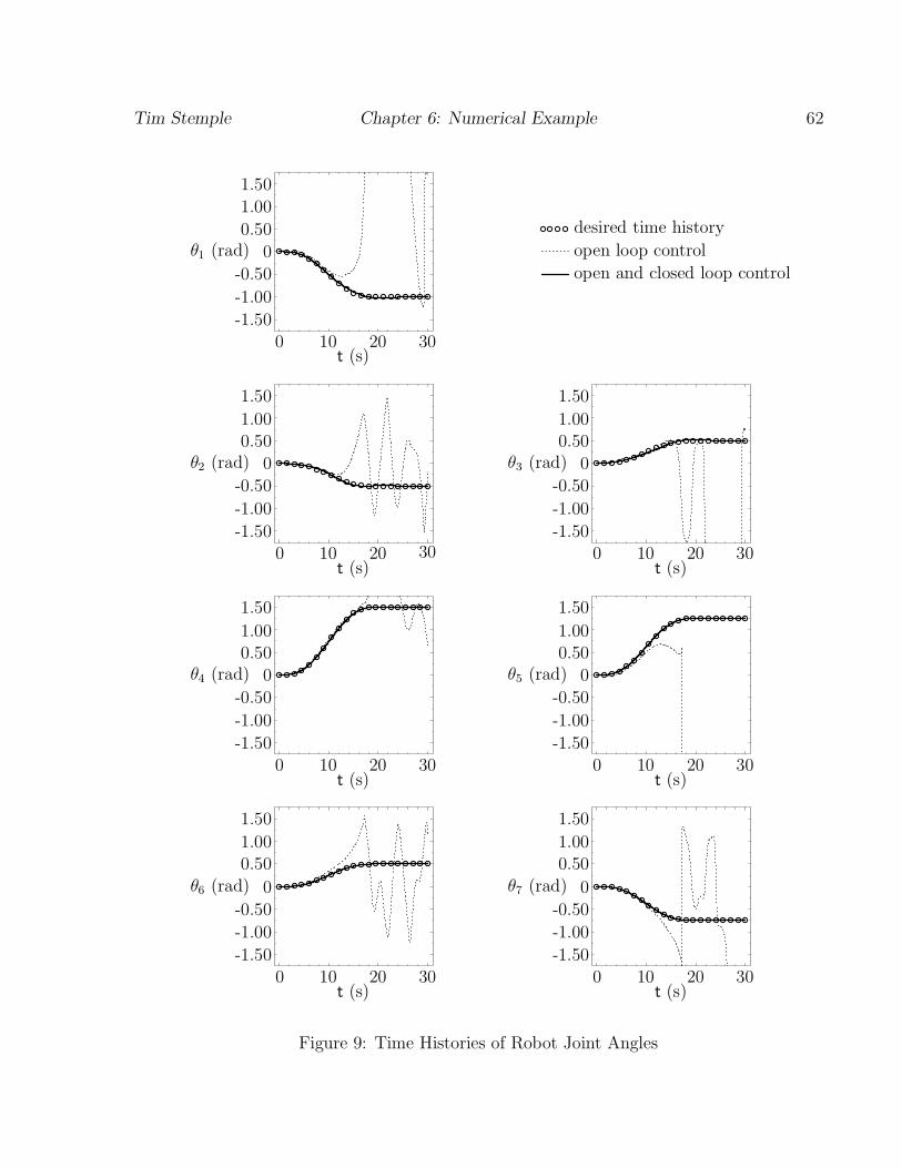
Tim Stemple Chapter 6: Numerical Example 62
1.50
1.00desired time history0.50open loop controlθ (rad) 01
open and closed loop control-0.50
-1.00
-1.500 10 20 30
t (s)
1.50 1.50
1.00 1.000.50 0.50
θ (rad) θ (rad)0 02 3
-0.50 -0.50
-1.00 -1.00
-1.50 -1.50300 10 20 0 10 20 30
t (s) t (s)
1.50 1.50
1.00 1.000.50 0.50
θ (rad) θ (rad)0 04 5
-0.50 -0.50
-1.00 -1.00
-1.50 -1.500 10 20 30 0 10 20 30
t (s) t (s)
1.501.50
1.001.000.500.50
θ (rad)θ (rad) 00 76
-0.50-0.50
-1.00-1.00
-1.50-1.500 10 20 300 10 20 30
t (s)t (s)
Figure 9: Time Histories of Robot Joint Angles
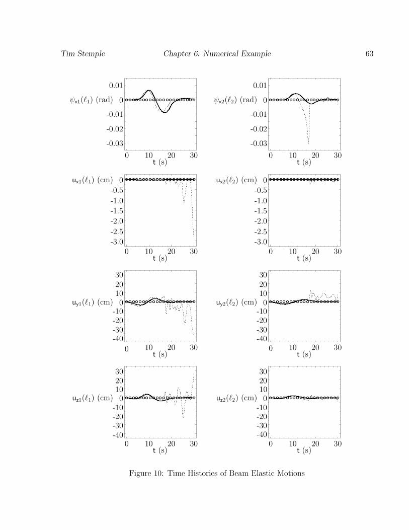
Tim Stemple Chapter 6: Numerical Example 63
0.01 0.01
ψ (` ) (rad) ψ (` ) (rad)0 0x1 1 x2 2
-0.01 -0.01
-0.02 -0.02
-0.03 -0.03
0 10 20 30 0 10 20 30t (s) t (s)
u (` ) (cm) u (` ) (cm)0 0x1 1 x2 2
-0.5 -0.5
-1.0 -1.0
-1.5 -1.5
-2.0 -2.0
-2.5 -2.5
-3.0 -3.00 10 20 30 0 10 20 30
t (s) t (s)
30 3020 2010 10
u (` ) (cm) u (` ) (cm)0 0y1 1 y2 2
-10 -10-20 -20-30 -30-40 -40
10 20 30 10 20 3000t (s) t (s)
30 3020 2010 10
u (` ) (cm) u (` ) (cm)0 0z1 1 z2 2
-10 -10-20 -20-30 -30
-40-400 10 20 30 0 10 20 30
t (s) t (s)
Figure 10: Time Histories of Beam Elastic Motions
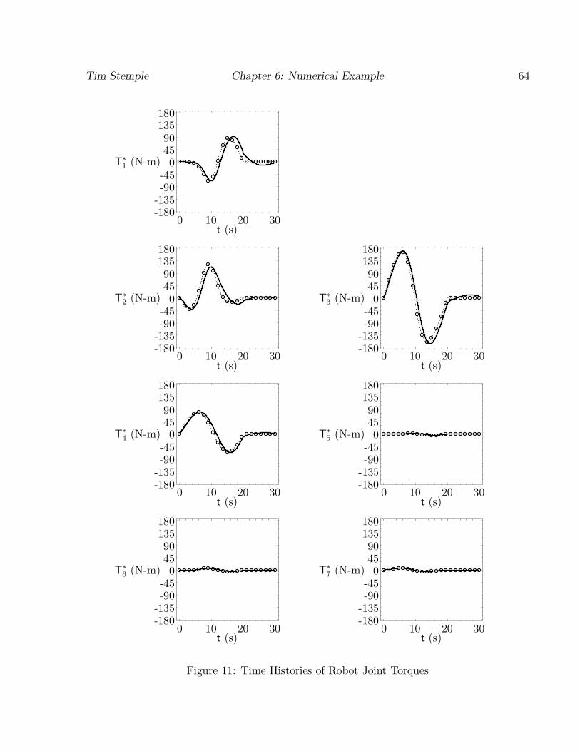
Tim Stemple Chapter 6: Numerical Example 64
1801359045
∗T (N-m) 01
-45-90
-135-180
0 10 20 30t (s)
180 180135 13590 9045 45
∗ ∗T (N-m) T (N-m)0 02 3
-45 -45-90 -90
-135 -135-180 -180
0 10 20 30 0 10 20 30t (s) t (s)
180 180135 13590 9045 45
∗ ∗T (N-m) T (N-m)0 04 5
-45 -45-90 -90
-135 -135-180 -180
0 10 20 30 0 10 20 30t (s) t (s)
180 180135 13590 9045 45
∗ ∗T (N-m) T (N-m)0 06 7
-45 -45-90 -90
-135 -135-180 -180
0 10 20 30 0 10 20 30t (s) t (s)
Figure 11: Time Histories of Robot Joint Torques
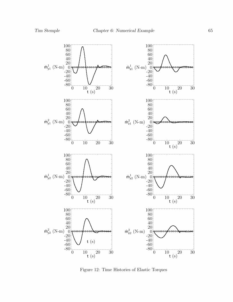
Tim Stemple Chapter 6: Numerical Example 65
100 10080 8060 6040 4020 20
1 1m (N-m) ˆ0 m (N-m) 0y1 z1-20 -20-40 -40-60 -60-80 -80
0 10 20 30 0 10 20 30t (s) t (s)
100 10080 8060 6040 4020 20
2 2m (N-m) ˆ0 m (N-m) 0y1 z1-20 -20-40 -40-60 -60-80 -80
0 10 20 30 0 10 20 30t (s)
100 10080 8060 6040 4020 20
1 1m (N-m) m (N-m)0 0y2 z2-20 -20-40 -40-60 -60-80 -80
0 10 20 30 0 10 20 30t (s) t (s)
100 10080 8060 6040 4020 20
2 2m (N-m) m (N-m)0 0y2 z2-20 -20-40 -40t (s)-60 -60-80 -80
0 10 20 30 0 10 20 30t (s) t (s)
Figure 12: Time Histories of Elastic Torques
Chapter 7 Summary and Conclusions
An efficient technique for generating equations of motion for flexible multibody structures,carried out by means of the Principle of Virtual Work, has been presented. The resultingformulation is quite general, and can be used to model the dynamics of a large class ofmultibody structures. In particular, open-loop structures comprised of rigid bodies andslender beams connected by any type of revolute joint can be modeled. The structure canhave one body fixed in the inertial space, or be freely floating. Furthermore, the joints canbe actively controlled, governed by the action of torsional springs and dampers, or torquefree. The model also allows for any type of control force or torque to be acting on the surfaceof the bodies.
Due to the modular nature of the computer program, it would be a simple exercise toextend the setup to include structures with prismatic joints, as well as structures moving ina gravitational field. As far as flexibiltiy models are concerned, the beams are modeled assecond-order Rayleigh beams. Not much work would be required, however, to extend theprogram to include second-order Timoshenko beam models in the class of structures whichcan be modeled.
The equations of motion are initially presented in hybrid variational form. That is,they include both generalized coordinates and quasi-velocities, which involve the rigid bodymotions, as well as functions of time and space which model the elastic motions of the flexiblebodies in the structure. A form of the hierarchical finite element method, which, for bending,uses the sequence of fixed-fixed Euler-Bernoulli eigenfunctions instead of polynomials for thehierarchical functions, was used to carry out the discretization process. In general, thehierarchical finite element method requires substantially fewer degrees of freedom than theusual, or h-version, of the finite element method. Furthermore, there are also advantagesto using eigenfunctions, as opposed to polynomials, as hierarchical functions. For one, theeigenfunctions by themselves are orthogonal, but also, when combined with the Hermite
66
Tim Stemple Chapter 7: Summary and Conclusions 67
cubics they enjoy a certain amount of additional orthogonality. The end result, of course, isthat the mass and stiffness matrices are substantially sparser. Another advantage to usingeigenfunctions, as opposed to polynomials, arises from what happens when the number ofhierarchical functions is increased. When using polynomials, there is a limit to the numberof hierarchical functions which can be used, since increasing this number causes the massmatrix to become more singular, causing the system to become numerically unstable. Thisphenomenon is postponed consideraby when using eigenfunctions as hierarchical functions.To be more precise, the hierarchical finite element method was applied to a four storyframed structure comprised of Euler-Bernoulli beams [46]. Using more than six polynomialsas hierarchical functions resulted in numerical instability, whereas when using eigenfunctions,there was no practical limit to the number of hierarchical functions which could be used.
We have also introduced a practical application of the exponential form of a properorthogonal matrix, which was used in converting general nonlinear slender beam equationsto a form involving up through second-order terms in the functions used to measure thedisplacement of a cross-section relative to body axes. The exponential form of the orthogonalmatrix is ideally suited to this operation, since the Taylor series of the exponential functionis straightforward and easily truncated.
A numerical example, which involves the motion of a flexible robot arm, was includedto demonstrate the effectiveness of the computer program. The structure consists of a rigidbase with two flexible arms and a rigid end-effector. However, since the main interest was inthe maneuvering of a payload from one location to another, the base was assumed fixed inthe inertial space. The joint control torques consist of an open loop plus closed loop torque.The open loop control torques were determined by requiring the structure, assumed rigid,to move in such a way that the joint angles follow specified trajectories. The closed loopportion of the control torque was determined locally. That is, for each of the joint angles,the closed loop control torque associated with that joint angle responded to the error in thedesired angular position and angular velocity.
The elastic motion of the beams was controlled with actuators capable of producingtorques about the y and z axes. The actuators are arranged in pairs, with the individualii
actuators of a given pair separated by a short distance, and producing torques of equalmagnitude but opposite sign. The control again is local, with the magnitude of the torqueof a given actuator pair responding to the curvature and time rate of change of curvature ofthe point midway between the two actuators. Four actuator pairs were located on each ofthe two beams, all situated at the ends of the beams, with two pairs exerting torques aboutthe y axis, and two pairs exerting torques about the z axis. An examination of the plotsii
of joint angle time histories and elastic displacement time histories shows that the controlstrategy certainly had the desired effect.
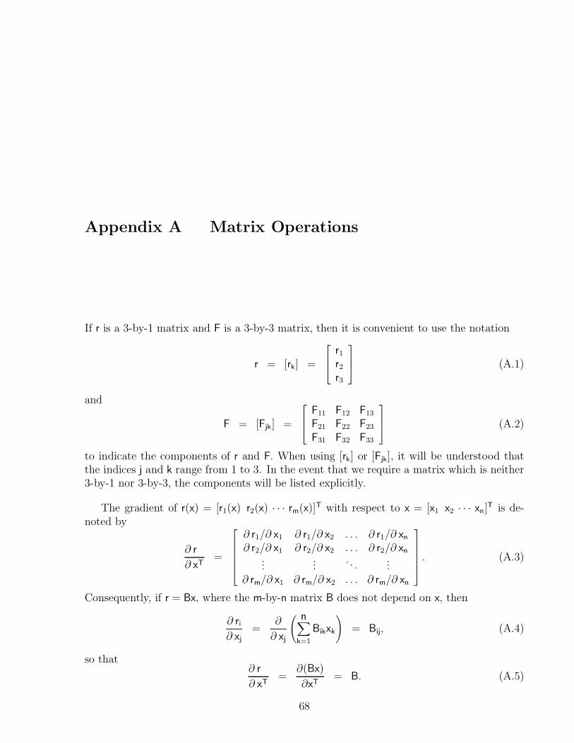
Appendix A Matrix Operations
If r is a 3-by-1 matrix and F is a 3-by-3 matrix, then it is convenient to use the notation r1 rr = [r ] = (A.1) k 2
r3
and F F F11 12 13 F F FF = [F ] = (A.2) jk 21 22 23
F F F31 32 33
to indicate the components of r and F. When using [r ] or [F ], it will be understood thatk jk
the indices j and k range from 1 to 3. In the event that we require a matrix which is neither3-by-1 nor 3-by-3, the components will be listed explicitly.
T TThe gradient of r(x) = [r (x) r (x) · · · r (x)] with respect to x = [x x · · · x ] is de-1 2 m 1 2 n
noted by ∂ r /∂ x ∂ r /∂ x . . . ∂ r /∂ x1 1 1 2 1 n ∂ r /∂ x ∂ r /∂ x . . . ∂ r /∂ x ∂ r 2 1 2 2 2 n = . (A.3). . .. T . . . .∂ x . . . .∂ r /∂ x ∂ r /∂ x . . . ∂ r /∂ xm 1 m 2 m n
Consequently, if r = Bx, where the m-by-n matrix B does not depend on x, then( )n∑∂ r ∂i= B x = B , (A.4)ik k ij
∂ x ∂ xj j k=1
so that∂ r ∂(Bx)
= = B. (A.5)T T∂ x ∂x
68
Tim Stemple Appendix A: Matrix Operations 69
Furthermore, if r depends on x (but not necessarily linearly, as above), and x depends onTy = [y y . . . y ] , then1 2 s
n∑∂ r ∂ r ∂ xi i k= , (A.6)
∂ y ∂ x ∂ ykj jk=1
so that the chain rule takes the form
∂ r ∂ r ∂ x= . (A.7)
T T T∂ y ∂ x ∂ y
˜If a = [a ], then the 3-by-3 skew-symmetric matrix Tilde(a) = a is defined byk 0 −a a3 2 Tilde(a) = a = a 0 −a (A.8-a) 3 1
−a a 02 1
˜= [(a) ] = −ε a , (A.8-b)jk jkm m
where ε is the permutation symbol, i.e., ε = ε = ε = 1, ε = ε = ε = −1,jkm 123 312 231 321 132 213
ε = 0 if i ∗ j ∗ k 6= 6, and we have made use of the Einstein summation convention. If B isijk
any 3-by-3 matrix, then it is a simple exercise to show that
T˜ ˜ ˜ ˜(Ba) = (TrB)a− B a− aB, (A.9)
where Tr stands for trace. Furthermore, if c is another 3-by-1 matrix, then letting B = c inEq. A.9 implies that ˜ ˜˜ ˜˜(ca) = ca− ac. (A.10)
˜Multiplying on the right by ca results in the left side equaling the 3-by-3 zero matrix, so that
2˜˜˜ ˜˜caca = ac a. (A.11)
Another easily verified fact isT˜˜˜ ˜aca = −(a c)a, (A.12)
which can then be used to prove that
2n+1 n T n˜ ˜a = (−1) (a a) a, (A.13-a)2n+2 n T n 2˜ ˜a = (−1) (a a) a , n = 0, 1, 2, . . . . (A.13-b)
The description of the motion of one coordinate system with respect to another is ofcentral importance in the dynamics of multibody systems. To begin with, let orthonormalbasis e , e , e be associated with a coordinate system with axes x x x and origin A, and1 2 3 1 2 3
orthonormal basis b ,b ,b be associated with a coordinate system with axes y y y and1 2 3 1 2 3
origin B. Next, define the time derivative of vector r with respect to axes x x x by1 2 3
d d dr = (r · e )e + (r · e )e + (r · e )e . (A.14)1 1 2 2 3 3
dt dt dt
Tim Stemple Appendix A: Matrix Operations 70
−→And then, let R = AB be the position vector of point B with respect to point A and Ω theangular velocity of axes y y y with respect to axes x x x .1 2 31 2 3
Note that Ω is given by
Ω = (b · b )b + (b · b )b + (b · b )b (A.15-a)2 3 1 3 1 2 1 2 3
1= ε (b · b )b , (A.15-b)ijk j k i2
which endows it with the usual property,
b = Ω× b , k = 1, 2, 3. (A.16)k k
We also introduce the four component matrices
R = [ R ] = [ R · e ], (A.17)k k
P = [P ] = [b · e ], (A.18)jk j k
V = [ V ] = [R · b ], (A.19)k k
Ω = [Ω ] = [Ω · b ], (A.20)k k
where we recognize that R contains the components of position vector R, along axes x x x ,1 2 3
P is the matrix of direction cosines of axes y y y with respect to axes x x x , and V and1 2 31 2 3 Ω contain, respectively, the components of velocity vector R and angular velocity vector Ω,both along axes y y y . Note that this definition of P implies that the 3-by-1 matrix PR1 2 3
contains the components of vector R, along axes y y y , and furthermore that1 2 3
e = (e · b )b = P b . (A.21)k k j j jk j
Then, making use of the easily verified fact that for any two vectors a and b, d(a · b)/dt =
a · b + a · b, we see that
˙ ˙R = [R ] = [d(R · e )/dt] = [R · e ] = [R · (P b )] = [P V ]k k k jk j jk j
T= P V, (A.22)
˙ ˙P = [P ] = [d(b · e )/dt] = [b · e ] = [(Ω× b ) · e ]jk j k j k j k
= [(b × e ) ·Ω] = [(b × P b ) ·Ω] = [P ε b ·Ω]j k j nk n nk jnm m˜= [P ε Ω ] = −[(−ε Ω )P ] = −[(Ω) P ]nk jnm m jnm m nk jn nk˜= −ΩP. (A.23)
Multiply Eq. A.22 on the left by P, and then rearrange Eq. A.23 by taking the transpose ofboth sides, and then multiplying on the left by P, to get that
˙V = PR, (A.24)T˜ ˙Ω = PP . (A.25)
Tim Stemple Appendix A: Matrix Operations 71
Two comments are in order. First, if we are given the matrices R and P, we can useEqs. A.24 and A.25 to define V and Ω, without regard to the physical meaning as components
of R and Ω. Secondly, we can replace the “dot” in Eqs. A.24 and A.25 with another operator.∗∗For example, we can define the quasi-virtual displacements δR and δΘ by
∗δR = PδR, (A.26)∗ TδΘ = PδP . (A.27)
We will have occasion to use some facts related specifically to matrices of directioncosines. Recall that the matrix of direction cosines P is a proper orthogonal matrix, i.e.,
T TP P = PP = I and det P = 1. Furthermore, it is well known that
2˜ ˜P = I− (sin φ)ξ + (1− cosφ)ξ , (A.28)
T 2 2 2in which φ is a scalar and ξ = [ ξ ξ ξ ] satisfies ξ + ξ + ξ = 1. In fact, φ is the angle of1 2 3 1 2 3Trotation about the axis defined by unit vector ξ = ξ e = ξ b . If a = [ a a a ] is any 3-by-1i i i i 1 2 3
matrix, then Eqs. A.12 and A.28 can be used to verify the identity
T˜ ˜(Pa) = PaP . (A.29)
Introducing the Taylor series for sin φ and 1− cosφ into Eq. A.28, we get that
∞ k k∑ (−1) θ ˜P = = exp(−θ), (A.30)k!
k=0
Tin which the 3-by-1 matrix θ = φξ = [φξ φξ φξ ] .1 2 3
TNext we assume that the orthogonal matrix P is a function of θ = [ θ θ θ ] . Then,1 2 3T T Tsince PP = I, we have that P(∂P /∂θ ) + (∂P/∂θ )P = 0, k = 1, 2, 3. This implies thatk k
TP(∂P /∂θ ) is a 3-by-3 skew-symmetric matrix, which allows the introduction of a 3-by-1kTmatrix β = [ β β β ] defined byk 1k 2k 3k
T∂Pβ = P , k = 1, 2, 3. (A.31)k
∂θk
Furthermore, the chain rule implies that ( )3 3 3T∑ ∑ ∑∂PT ˜˙ ˙ ˙ ˙PP = P θ = β θ = Tilde β θk k k k k
∂θkk=1 k=1 k=1˜= (Dθ), (A.32)
in which β β β11 12 13[ ]. .. . . .. .D = β β β = β β β . (A.33) 21 22 231 2 3. .. .β β β31 32 33
Tim Stemple Appendix A: Matrix Operations 72
Applying this procedure to the characterization of P given in Eq. A.28 and taking into√T 2 2 3account that ξ = [ θ /φ θ /φ θ /φ ] where φ = θ + θ + θ , it can be shown that1 2 3 1 2 3
sin φ φ− sinφ 1− cosφ˜β = e + θ θ + e θ, (A.34)k k k k3 2φ φ φ
which, when substituted into Eq. A.33 can be shown to yield the formula
1− cosφ φ− sinφ 2˜ ˜D = I− θ + θ . (A.35)2 3φ φ
This closed-form expression for D is akin to that given for P in Eq. A.28. Introducing Taylor2 3series expansions for (1− cosφ)/φ and (φ− sin φ)/φ into Eq. A.35 and making use also of
Eqs. A.13-a and A.13-b, we get that the Taylor series expansion for D is given by
∞ k k∑ (−1) θD = , (A.36)
(k + 1)!k=0
which, except for the k+1 in the denominator, is identical to the Taylor series formula for P.It is also possible to verify the identity of Eq. A.32 directly from the Taylor series formulasfor P (Eq. A.30) and D (Eq. A.36), although the proof is not particularly straightforward.
There are two facts concerning the trace of a square matrix which will be required. If Aand B are both n-by-n matrices, then it is easy to verify that
Tr[AB] = Tr[BA], (A.37)
and if S and W are n-by-n matrices, with S symmetric and W skew-symmetric, then
Tr[SW] = 0. (A.38)
Finally, we will also need a simple formula related to the component matrix of the gradientof a vector valued function z(r). Let z = [z ] be the component matrix of z, along axesk
x x x , and r = [r ] the component matrix of r, along axes y y y . Suppose we are given1 2 3 k 1 2 3Tz = [z ] as a function of r = [r ], so that it is straightforward to compute ∂z/∂r , but requirek k
the component matrix F of the gradient ∇z with respect to axes x x x . Recall that by1 2 3T Tdefinition [16], F = ∂z/∂ r , in which r = P r is the component matrix of r, along axes x x x1 2 3
and P is the matrix of direction cosines of axes y y y with respect to axes x x x . This1 2 31 2 3
¯implies that r = Pr, and consequently,
¯∂z ∂z ∂r ∂z ∂(Pr) ∂zF = = = = P, (A.39)
T T TT T T¯ ¯ ¯∂r ∂r ∂r ∂r ∂r ∂r
which is the desired formula.
Bibliography
[1] Agrawal, O. P., “General Approach to Dynamic Analysis of Rotorcraft,” Journal ofAerospace Engineering , Vol. 4, No. 1, 1991, pp. 99-107.
[2] Amirouche, F. M. L. and Xie, M., “Explicit Matrix Formulation of the DynamicalEquations for Multibody Systems: A Recursive Approach,” Computers and Structures,Vol. 46, No. 2, 1993, pp. 311-321.
[3] Avello, A., De Jalon, J. G. and Bayo, E., “Dynamics of Flexible Multibody SystemsUsing Cartesian Co-ordinates and Large Displacement Theory,” International Journalfor Numerical Methods in Engineering , Vol. 32, No. 8, 1991, pp. 1543-1563.
[4] Baruh, H. and Tadikonda, S. S. K., “Issues in the Dynamics and Control of FlexibleRobot Manipulators,” Journal of Guidance, Control, and Dynamics , Vol. 12, No. 5,1989, pp. 659-671.
[5] Bayo, E., Papadopoulos, P., Stubbe, J. and Serna, M. A., “Inverse Dynmaics andKinematics of Multi-Link Elastic Robots: An Iterative Frequency Domain Approach,”The International Journal of Robotics Research, Vol. 8, No. 6, 1989, pp. 49-62.
[6] Book, W. J., Maizza-Neto, O. and Whitney,“Feedback Control of Two Beam, TwoJoint Systems with Distributed Blexibility,” Journal of Dynamic Systems, Measure-ment, and Control , 1975, pp. 424-431.
[7] Book, W. J., “Recursive Lagrangian Dynamics of Flexible Manipulator Arms,” TheInternational Journal of Robotics Research, Vol. 3, No. 3, 1984, pp. 87-101.
[8] Cavin, R. K., III and Dusto, A. R., “Hamilton’s Principle: Finite-Element Methods andFlexible Body Dynamics,” AIAA Journal , Vol. 15, No. 12, December 1977, pp. 1684-1690.
[9] Chan, J. K. and Modi, V. J., “Dynamics and Control of an Orbiting Flexible MobileManipulator,” Acta Astronautica, Vol. 21, No. 11-12, 1990, pp. 759-769.
73
Tim Stemple Bibliography 74
[10] Chang, C. W. and Shabana, A. A., “Spatial Dynamics of Deformable Multibody Sys-tems with Variable Kinematic Strucure, Part 1. Dynamic Model & Part 2. VelocityTransformation” Journal of Mechanisms, Transmissions, and Automation in Design,Vol. 112, No. 2, 1990, pp. 153-167.
[11] Chen, Y. and Meirovitch, L., “Control of a Flexible Space Robot During a DockingManeuver,” Journal of Applied Mechanics , Vol. 55, 1988, pp. 687-693.
[12] Cyril, X., Angeles J. and Misra, A., “Dynamics of Flexible Multibody MechanicalSystems,” Transaction of the Canadian Society for Mechanical Engineers , Vol. 15,No. 3, 1991, pp. 235-256.
[13] de Veubeke, B. F., “The Dynamics of Flexible Bodies,” International Journal of En-gineering Science, Vol. 14, 1976, pp. 895-913.
[14] Garcia, E. and Inman, D. J., “Advantages of Slewing an Active Structure,” Journal ofIntelligent Material Systems and Structures , Vol. 1, July, 1990, pp. 261-272.
[15] Geradin, M., Cardona, A. and Granville, D., “Finite Element Modeling of FlexibleMultibody Systems,” The International Symposium on Advanced Computers for Dy-namics and Design, ACD & D ’89-B08, 1989, pp. 219-224.
[16] Gurtin, M. E., An Introduction to Continuum Mechanics, Academic Press, 1981.
[17] Haug, E. J., Computer Aided Kinematics and Dynamics of Mechanical Systems , Allynand Bacon, Boston, 1989.
[18] Ho, J. Y. L., “Direct Path Method for Flexible Multibody Spacecraft Dynamics,”Journal of Spacecraft and Rockets, Vol. 14, No. 2, 1977, pp. 102-110.
[19] Hughes, P. C., “Dynamics of a Chain of Flexible Bodies,” The Journal of the Astro-nautical Sciences , Vol. XXVII, No. 4, 1979, pp. 359-380.
[20] Huston, R. L., Multibody Dynamics, Butterworth-Heinemann, Boston, 1990.
[21] Ider, S. K., “Finite-Element Based Recursive Formulation for Real Time DynamicSimulation of Flexible Multibody Systems,” Computers and Structures, Vol. 40, No. 4,1991, pp. 939-945.
[22] Kane, T. R. and Levinson, D. A., “Formulation of Equations of Motion for ComplexSpacecraft,” Journal of Guidance and Control , Vol. 3, No. 2, 1980, pp. 99-112.
[23] Kane, T. R. and Levinson, D. A., “The Use of Kane’s Dynamical Equations inRobotics,” The International Journal of Robotics Research, Vol. 2, No. 3, 1983, pp. 3-21.
Tim Stemple Bibliography 75
[24] Keat, J. E., “Multibody System Order n Dynamics Formulation Based on VelocityTransform Method,” Journal of Guidance, Control, and Dynamics , Vol. 13, No. 2,1990, pp. 207-212.
[25] Kim, S. S. and Haug, E. J., “Recursive Formulation for Flexible Multibody Dynamics,Part I: Open-Loop Systems”, Computer Methods in Applied Mechanics and Engineer-ing , Vol. 71, No. 3, 1988, pp. 293-314.
[26] Koppens, W. P., Sauren, A. A. H. J., Veldpaus, F. E. and VanCampen, D. H., “Dy-namics of a Deformable Body Experiencing Large Displacements”, Journal of AppliedMechanics, Vol. 55, No. 3, 1988, pp. 676-680.
[27] Kwak, M. K. and Meirovitch, L., “New Approach to the Maneuvering and Control ofFlexible Multibody Systems,” Journal of Guidance, Control, and Dynamics, Vol. 15,No. 6, 1992, pp. 1342-1353.
[28] Lai, H.-J., Haug, E., Kim, S.-S. and Bae, D. S., “Decoupled Flexible-Relative Coor-dinate Recursive Approach for Flexible Multibody Dynamics,” International Journalfor Numerical Methods in Engineering/, Vol. 32, No. 8, 1991, pp. 1669-1689.
[29] Lieh, J., “Separated-Form Equations of Motion of Controlled Flexible Multibody Sys-tems,” Journal of Dynamic Systems, Measurement and Control , Vol. 116, No. 4, 1994,pp. 702-712.
[30] Low, K. H.,“A Systematic Formulation of Dynamic Equations for Robot Manipulatorswith Elastic Links,” Journal of Robotic Systems , Vol. 4, No. 3, 1987, pp. 435-456.
[31] Marsden, J. E. and Hughes, T. R., Mathematical Foundations of Elasticity, Prentice--Hall, INC., Englewood Cliffs, NJ, 1983.
[32] Meirovitch, L., Methods of Analytical Dynamics, McGraw-Hill Book Co., New York,1970.
[33] Meirovitch, L., “Hybrid State Equations of Motion for Flexible Bodies in Terms ofQuasi-Coordinates,” Journal of Guidance, Control, and Dynamics, Vol. 14, No. 5,1991, pp. 1008-1013.
[34] Meirovitch, L., “Derivation of Equations for Flexible Multibody Systems in Termsof Quasi-Coordinates from the Extended Hamilton’s Principle,” Shock and Vibration,Vol. 1, No. 2, 1993, pp. 107-119.
[35] Meirovitch, L., Principles and Techniques of Vibrations, Prentice Hall, EnglewoodCliffs, NJ, 1996.
[36] Meirovitch, L. and Chen, Y., “Trajectory and Control Optimization for Flexible SpaceRobots,” Journal of Guidance, Control, and Dynamics, Vol. 18, No. 3, 1995, pp. 493-502.
Tim Stemple Bibliography 76
[37] Meirovitch, L. and Kwak, M. K., “Control of Spacecraft with Multi-Targeted FlexibleAntennas,” Journal of the Astronautical Sciences, Vol. 38, No. 2, 1990, pp. 187-199.
[38] Meirovitch, L. and Kwak, M. K., “Rayleigh-Ritz Based Substructure Synthesis forFlexible Multibody Systems,” AIAA Journal, Vol. 29, No. 10, 1991, pp. 1709-1719.
[39] Meirovitch, L. and Lim, S., “Maneuvering and Control of Flexible Space Robots,”Journal of Guidance, Control, and Dynamics, Vol. 17, No. 3, 1994, pp. 520-528.
[40] Meirovitch, L. and Nelson, H. D., “On the High-Spin Motion of a Satellite ContainingElastic Parts,” Journal of Spacecraft and Rockets, Vol. 3, No. 11, 1966, pp. 1597-1602.
[41] Meirovitch, L. and Quinn, R. D., “Equations of Motion for Maneuvering FlexibleSpacecraft,” Journal of Guidance, Control, and Dynamics, Vol. 10, No. 5, 1987,pp. 453-465.
[42] Meirovitch, L. and Stemple, T. J., “Dynamics and Control of Flexible Multibody Sys-tems,” Proceedings of the First Joint Conference of International Simulation Societies,August 1994, Zurich, Switzerland, pp. 268-272.
[43] Meirovitch, L. and Stemple, T., “Hybrid Equations of Motion for Flexible Multi-body Systems Using Quasi-Coordinates,” Journal of Guidance, Control and Dynamics ,Vol. 18, No. 4, 1995, pp. 678-688.
[44] Meirovitch, L. and Stemple, T. J., “Maneuvering and Control of Flexible Robots,”Proceedings of the 5th International Conference on Advances in Communication andControl , June 1995, Crete, Greece.
[45] Meirovitch, L. and Stemple, T. J., “Simulation of Three-Dimensional Maneuver andControl of Flexible Multibody Systems,” June 1996, Budapest, Hungary.
[46] Meirovitch, L. and Stemple, T. J., “Nonlinear Control of Structures in Earthquakes,”Structural Dynamics and Control, Proceedings of the 11th VPI&SU Symposium,May 1997, Blacksburg, VA.
[47] Naganathan, G. and Soni, A. H., “Nonlinear Modeling of Kinematic and Flexibility Ef-fects in Manipulator Design,” Journal of Mechanisms, Transmissions, and Automationin Design, Vol. 110, No. 3, 1988, pp. 243-254.
[48] Nikravesh, P. E. and Ambrosio, J. A. C., “Systematic Construction of Equations ofMotion for Rigid-Flexible Multibody Systems Containing Open and Closed KinematicLoops,” International Journal for Numerical Methods in Engineering , Vol. 32, No. 8,1991, pp. 1749-1766.
[49] Pereira, M. S. and Proenca, P. I., “Dynamics Analysis of Spatial Flexible MultibodySystems Using Joint Co-ordinates,” International Journal for Numerical Methods inEngineering , Vol. 32, No. 8, 1991, pp. 1799-1812. Vol. 15, No. 2, 1992, pp. 390-395.
Tim Stemple Bibliography 77
[50] Quinn, R. D., “Equations of Motion for Structures in Terms of Quasi-Coordinates,”Journal of Applied Mechanics, Vol. 57, 1990, pp. 745-749.
[51] Roberson, R. E. and Schwertassek, R., Dynamics of Multibody Systems, Springer-Ver-lag, Berlin, 1988.
[52] Rogers, Robert C., “Derivation of Linear Beam Equations Using Non-Linear Contin-uum Mechanics,” Journal of Applied Mathematics and Physics (a.k.a. ZAMP), Vol. 44,No. 4, July 1993, pp. 732-754.
[53] Shabana, A. A., Dynamics of Multibody Systems , Wiley, New York, 1989.
[54] Shabana, A. A., “Dynamics of Flexible Bodies Using Generalized Newton-Euler Equa-tions,” Journal of Dynamic Systems, Measurement and Control , Vol. 112, No. 3, 1990,pp. 496-503.
[55] Shabana, A. A., “Constrained Motion of Deformable Bodies,” International Journalfor Numerical Methods in Engineering , Vol. 32, No. 8, 1991, pp. 1813-1831.
[56] Simo, J. C. and Vu-Quoc, L., “A Three-Dimensional Finite-Strain Rod Model. Part II:Computational Aspects,” Computer Methods in Applied Mechanics and Engineering,Vol. 58, 1986, pp. 79-116.
[57] Suleman, A., Modi, V. J. and Venkayya, V. B., “Structural Modeling Issues in FlexibleSystems,” AIAA Journal , Vol. 33, No. 5, 1995, pp. 919-923.
[58] VanWoerkom, P. T. L. M., “Modified Dynamics for Maneuvering Flexible Space Ma-nipulators,” Journal of Sound and Vibration, Vol. 179, No. 5, 1995, pp. 777-792.
[59] VanWoerkom, P. T. L. M. and de Boer, A., “Development and Validation of a Lin-ear Recursive ‘Order-N ’ Algorithm for the Simulation of Flexible Space ManipulatorDynamics,” Acta Astronautica, Vol. 35, No. 2/3, 1995, pp. 175-185.
[60] Vukasovic, N., Celigueta, J. T. and de Jalon, J. G., “Flexible Multibody DynamicsBased on a Fully Cartesian System of Support Coordinates,” Journal of MechanicalDesign, Vol. 115, No. 2, 1993, pp. 294-299.
[61] Vu-Quoc, L. and Simo, J. C., “Dynamics of Earth-Orbiting Flexible Satellites withMultibody Components,” Journal of Guidance, Control, and Dynamics , Vol. 10, No. 6,1987, pp. 549-558.
[62] Wallrapp, O. and Schwertassek, R., “Representation of Geometric Stiffening Effectin Multibody System Simulation,” International Journal for Numerical Methods inEngineering , Vol. 32, No. 8, 1991, pp. 1833-1850.
[63] Weng, S.-L. and Greenwood, D. T., “General Dynamical Equations of Motion forElastic Body Systems,” Journal of Guidance, Control, and Dynamics , Vol. 15, No. 6,1992, pp. 1434-1442.
Tim Stemple Bibliography 78
[64] Wittenburg, J., Dynamics of Systems of Rigid Bodies, B. G. Teubner, Stuttgart, 1977.
[65] Yamada, K., Tsuchiya, K. and Ohkami, Y., “Dynamical Models for a Flexible Multi-body System,” Control - Theory and Advanced Technology , Vol. 4, No. 1, 1988, pp. 37-51.
[66] Yoo, W. S. and Haug, E. J., “Dynamics of Articulated Structures. Part I. Theory,”Journal of Structural Mechanics, Vol. 14, No. 1, 1986, pp. 105-126.
[67] Yoo, W. S. and Haug, E. J., “Dynamics of Articulated Structures. Part II. ComputerImplementation and Applications,” Journal of Structural Mechanics , Vol. 14, No. 2,1986, pp. 177-189.
[68] Zhang, D. J., Liu, C. Q. and Huston, R. L., “On the Dynamics of an Arbitrary FlexibleBody with Large Overall Motion: An Integrated Approach,” Mechanics of Structuresand Machines, Vol. 23, No. 3, 1995, pp. 419-438.
VITA
Timothy J. Stemple was born at the Nouasseur Air Force base hospital near Casablanca, Mo-rocco. He received a B.S. and M.S. in mathematics from the University of Illinois (Urbana)and an M.S. from the Civil Engineering and Mechanics department at Southern Illinois Uni-versity (Carbondale). Subsequently, he enrolled in the ESM department at Virginia Tech,and has since been working to satisfy the requirements for the Ph.D. degree. He has also hadthe opportunity to teach: mathematics at the University of Illinois, dynamics at SouthernIllinois University, and both mathematics and statics at Virginia Tech.