Dynamic Effects of Price Promotions: A Large-ScaleField Experiment∗

Andrés Elberg† Pedro M. Gardete‡ Rosario Macera§ Carlos Noton¶

January 2016

Abstract

We investigate whether promotion depth has dynamic effects on subsequent pro-

motion sensitivity. In a large-scale field experiment we vary the promotion depth of

top sale products across 17 categories in 12 supermarket stores. During the first half

of the experiment we manipulate promotion depth by assigning staggered promotions

with 30% and 10% discounts to treated and control stores, respectively. In the second

half the staggering scheme assigns an even 10% to all stores. We find that treated

customers are 14% more likely to buy promoted items during the second half of the

experiment, and that the basket proportion of promoted items bought increases in

approximately 21%. This purchase behaviour is consistent with a model of sequential

search in which higher discounts alter the beliefs of rational consumers, who favours

search over promoted items during the second half. The heightened promotion sensi-

tivity leaves retailers facing a sort of prisoners dilemma: every retailer would be better

off in the absence of promotions, deviations, however, are profitable.

∗We thank Claudio Palominos for outstanding research assistance, as well as the participants in theRady Field Experimentation Conference, the Workshop in Consumer Analytics and Bryan Bollinger, WesleyHartmann, James Lattin, Harikesh Nair and Stephan Seiler for useful comments.†Universidad Diego Portales, Economics Department; andres.elberg@udp.cl‡Stanford University, Graduate School of Business; gardete@stanford.edu§Pontificia Universidad Católica, School of Business; rosario.macera@uc.cl¶University of Chile, Dept of Industrial Engineering, Center for Applied Economics; cnoton@dii.uchile.cl

1

1 Introduction

Consider the case of a hypothetical pair of customers, Mr. A and Mr. B, who are in allidentical, except they face different promotional discounts. Suppose Mr. A is offered adeep discount, while Mr. B finds only a shallow one. In most cases we would expect Mr.A to be more likely to buy than Mr. B, according for example with the standard law ofdemand. What happens however, when Mr. A and Mr. B face subsequent promotions? Inparticular, could differences in past promotion discounts affect how these customers perceiveand respond to future ones?

The effect of the exposure to promotions on consumers’ sensitivity to future promotionsis an open question. On the one hand, some managers believe that having become accus-tomed to deep promotions, the consumer will become less sensitive to subsequent promotionsrefraining thus from buying until he faces an attractive promotion again. In this case thefirm is required to offer greater promotional incentives over time to induce the same initialbuying behavior from the customer. Managers often refer to this habituation as deal addic-tion, because incentives need to be ratcheted up to maintain buying behavior. On the otherhand, and just as intuitively, it is also possible that deep promotions induce the costumer tobecome more sensitive to subsequent promotions, and in this case he would require smallerpromotional incentives after having received a large one to maintain his purchasing behavior.In this case, costumers are said to display inertia.

While deal addiction is certainly bad for business, it is not entirely clear that inertiais good for business. This is because managers are concerned that offering deep discountsmay “train” consumers to become deal seekers in the future, thus potentially hurting profits.Moreover, deal seekers may disregard other differentiating characteristics, and thus aggre-gate demand could become less heterogeneous, affecting different equilibrium outcomes inthe market. The implications of this claim are extremely broad, as they affect firms’ deci-sions about pricing (Anderson and Simester, 2004, 2010), about promotions and advertising(Erdem, Keane, and Sun, 2008), and may also affect firms’ understanding of heterogeneityof consumer responses to several marketing mix decisions (Chan, Narasimhan, and Zhang,2008). Even if the promotions train deal seekers, it remains relevant to investigate theunderlying mechanisms as well as the profitability implications for firms.

This paper investigates the phenomenon of heightened promotion sensitivity by imple-

2

menting a large field experiment in the retail sector. In conjunction with one of the majorretail chains in Chile, we exogenously vary the prices of 170 products across 17 top categoriesacross 12 stores to study how the depth of price discounts affects subsequent promotion sen-sitivity. Moreover, we take advantage of the individual level data available from the retailer’sloyalty card program to ensure comparing similar individuals in treated and control stores.

Our experiment is organized into two halves. In the first half, products in 6 treated storesreceived a “deep” 30% discount while the same products received a “shallow” 10% discountin the similar 6 control stores. All the remaining prices were identical across treated andcontrol stores. In the second half all stores were attributed an identical 10% discount. Giventhe design, we look for systematic consumer behavior differences during the second half ofthe experiment. We find that customers exposed to 30% discount promotions during thefirst half of the experiment became more willing to buy promoted items during the secondhalf than their control counterparts, despite the fact that during the second half promotiondepths were held constant across all stores. In particular, treated customers were 14% morelikely to buy promoted items during the second half of the experiment than their controlcounterparts. Moreover, the increase affects the basket composition of promoted vs. non-promoted items: Exposure to deep promotions increased the proportion of promoted goodsin consumers’ baskets by 20.5%.

Previous studies of the relationship between promotion activity and subsequent consumerbehavior include, among others, Mela, Gupta, and Lehmann (1997) and Jedidi, Mela, andGupta (1999).1 Mela, Gupta, and Lehmann (1997) use a discrete choice model with time-varying parameters and document that in the long-run price promotions are associated withheightened price sensitivity of both loyal and non-loyal customers. Jedidi, Mela, and Gupta(1999) take advantage of the same long series analyzed in Mela, Gupta, and Lehmann (1997)and show that promotions are associated with negative brand equity. A feature of thesestudies that makes causal inference difficult is that they rely on naturally generated scannerdata to identify the effect of promotion activity on future consumer behavior.

In contrast to this literature, and to the best of our knowledge, this paper is the first oneto provide experimental evidence of the link between promotional activity and promotionsensitivity in a physical retail setting where the prices of a large set of products is exogenouslymanipulated over time. This allow us to provide an unbiased estimate of the causal effect

1See Neslin and Van Heerde (2008) for an extensive review on promotion dynamics.

3

of promotional depth on subsequent purchase behavior of customers, addressing the naturalendogeneity issue present in transactional data.

The closest work to ours is Anderson and Simester (2004) who randomize prices in mailorder catalogs selling durable goods to study the long-run effects of the depth of pricediscounts over subsequent customer orders. They find that new customers who are offereddeeper discounts exhibit larger orders in subsequent purchases relative to the control group.In contrast, established customers react in the opposite way by reducing their subsequentpurchases.

Our results complement those in Anderson and Simester (2004) as both our context andexperimental design display important differences. First, we analyze frequently purchasedpackaged goods in a supermarket environment, rather than durable goods in a mail or-der catalog context. This is important as some of the mechanisms explaining consumers’responses to promotion activity (e.g., learning) are likely to depend on the nature of thegoods whose prices are being discounted. Second, and more importantly, our focus is onhow promotion sensitivity is affected by the depth of past promotions, rather than on howoverall purchase levels or subsequent regular price elasticities are affected by the depth ofpast promotions. In contrast, Anderson and Simester’s main focus is on subsequent reactionsto price rather than to promotions.2 Finally, Anderson and Simester (2004) focus on longrun effects (approximately two years), whereas ours are short run (over one month).

Our paper presents other unique features vis-à-vis the current literature. Because of thespecificities of our retail setting, we are able to rule out additional competing explanationssuch as state dependence and stockpiling behavior, and present robustness checks. Second,we propose our findings can be explained by a consumer search process, through which con-sumers optimally allocate their resources (i.e., time and effort) using their past beliefs toevaluate alternatives. We find that the beliefs implied by the past promotional activitiesare consistent with the search explanation, and derive the implications for competing man-ufacturers. The findings suggest that heightened promotion sensitivity fall into the class

2Even though Anderson and Simester (2004) also investigate deal sensitivity, they openly acknowledgethat their design is not particularly well suited for this purpose, as they did not explicitly manipulate thetiming of subsequent promotions. This implies that their measured treatment effect in this regard can becontaminated by endogenous forces (e.g., manufacturers/retailer may be responding to demand shocks duringthe second half of the experiment), unlike in our case. In effect, Anderson and Simester (2004) suggest ourfocus as a possible avenue for future research: “We cannot say how customers would have responded to [..]a subsequent discount. Investigating these issues would require different studies in which the experimentalmanipulations were [..] repeated in a subsequent catalog”.

4

of Bertrand supertraps explained by Cabral and Villas-Boas (2005), in which an apparentadvantage (such as scope economies) for one firm can lead to lower profits (through fiercercompetition) to competing firms.

2 Experimental Design

2.1 Intervention

We partnered with a large chain of supermarkets to conduct this field experiment. The retailfirm is one of the two largest supermarkets chains in Chile commanding a market share onthe order of 30 percent nationwide. Its retail stores are organized into two retail sub-chains,which make use of different branding and perform separate marketing activities. Moreover,these retail chains encompass stores of different sizes with different marketing positions.Retail chain 1 includes large standalone supermarkets whereas retail chain 2’s supermarketsare smaller and are often located well within densely populated neighborhoods. We ran theexperiment simultaneously in both chains. However, as we discuss below, the interventionfailed to produce statistically significant results for stores of sub-retail chain 2. Given thatall results are directionally consistent across experiments, we believe that the smaller sizesof stores of chain 2 are at least partially responsible for failing to the produce statisticallysignificant effects. Hence, we focus most of the analysis on sub-chain 1. We report the maineffects for both sub-chains, and proceed with the analysis by focusing on sub-chain 1.3

The experimental intervention involved manipulating prices across stores of the twochains.4 In particular, the intervention involved assigning timing and depth of promotionsto 170 top-sale products belonging to 17 categories.5 Within each category, and in order tomaximize the “visibility” of the intervention, we randomly selected 10 products (or SKU’s)from the subset of 15 products exhibiting the largest market shares in each category.

In order to analyze the intertemporal response to varying promotion depth, we dividedthe total experimental period of 10 weeks into two sub-periods of equal length and randomlyassigned stores to two alternative conditions: (i) a high-discount condition in which the

3The remaining results for chain 2 are available from the authors.4See Table 5 for store identifiers and the corresponding chains.5The categories included in the study are the following: soft drinks, coldcuts, bottled water, pasta,

cookies, juice, yogurt, cooking oil, meat, breakfast cereal, milk UHT, packaged bread, cheese, snacks, beer,chocolates and tea.

5

participating products featured a 30 percent discount from their regular price over the firstfive weeks of the experimental period and a 10 percent discount from their regular priceover the last five weeks of the experiment; and (ii) a low-discount condition, in which theparticipating products featured 10 percent discounts from their regular price for the whole 10weeks of the experimental period.6 In what follows we refer to stores assigned to the high-discount condition as treated stores and to stores assigned to the low-discount conditionas the control stores. This design allows us to study how consumers who faced differentdiscounts in the past (first half of the experiment) respond to subsequent promotion stimuliof the same magnitude (second half). In particular, because promotion timing and depthare held constant across stores during the second half of the experiment, our focus is toidentify whether treated customers are more sensitive to the same promotions than theircontrol counterparts.

The discounts of 30 percent and 10 percent are near the upper and lower bounds of therange of discounts typically applied by the retailer in the past. We wanted the discounts to beas close as possible to these bounds in order to maximize the visibility of the intervention.In addition, we wanted the low discount to be different from zero in order to be able toseparate the pure promotion effect from a price effect.

Following the retailer’s typical practice, each product remained in the promotion condi-tion for one week. Products were placed on promotion on a Tuesday and remained in thatcondition until Monday of the following week. Since it was impractical to set all 10 prod-ucts in a category on promotion simultaneously, and because we wanted the high-discountcondition to remain in place for the full first-half of the experiment, we rotated the productsto be promoted within each category. This process is illustrated in Figure 1. Each color inFigure 1 represents a different pair of SKU’s within a given category. In each of the first fiveweeks of the experiment the price of two different SKU’s were marked down (30 percent inthe store assigned to the high-discount condition and 10 percent in the store assigned to thelow-discount condition). By the end of week five, the prices of all participating SKU’s hadbeen intervened with. This process was repeated in the second half of the experiment, thistime with equal mark downs of 10 percent in both types of stores, and (mostly) preservingthe same order in which the SKU’s were promoted in the first half of the intervention.

6Notice that regular prices at the treated and control stores are the same as the retailer set regular pricesbased on “pricing zones”, and both stores within a matched store-pair belong to the same pricing zone.

6

The setup relied on a laborious physical change of prices in stores, according to a givenschedule. The company’s management involved the store managers in the experiment. Man-agers were asked to write back to headquarters and also submit photos of updated pricepromotions on a weekly basis, as depicted in Figure 2. Given that managers are oftenlimited to the extent of the promotions they can offer, the experiment was generally wellreceived even by managers of control stores who were allowed to discount products by only10%. Managers receiving the 30% discount were explicitly told to avoid any additional actionto take advantage of the advantageous promotion.

2.2 Analysis

To increase the precision of our estimates we relied on a pairwise randomized design (seefor example Imbens, 2011) over similar stores along three dimensions: (i) similar consumerdemographics (age, gender, socioeconomic group); (ii) similar competition intensity; (iii)comparative geographic location. We used historical data from the retailer’s loyalty cardprogram to classify stores according to demographic similarity. Information on the level ofcompetition facing each store was provided and discussed with the retailer. The firm itselfclassifies each store into one of three levels of competition depending on the number and typeof rival stores located within a certain radius of its store. After concluding the matchingprocess one of the stores in each pair was randomly assigned into one of the two conditionsdescribed above by coin flip.7

The experiment is enriched by the availability of individual-level data, enabled by thewidespread use of loyalty cards. Consumers enrolled in the brand loyalty card purchaseabout 80% of the supermarket sales. These data improve the analysis at two levels. First,they allow us to reduce experimental noise by including pre-experimental behavior-basedmeasures in the analysis. These types of measures are well known to outperform othercontext-independent measures such as demographic characteristics. Second, they allow us toinvestigate heterogeneity by analyzing the distribution of treatment effects across individuals.

7Conversations with managers prior to the experiment revealed that logistical reasons made the promotionschedule of a few products in the experimental set challenging during the second half of the experiment, andso these products were promoted outside the promotion schedule in Figure 1. While these products didnot follow the original promotion schedule, we still correctly incorporate their promotions into the analysisbecause the promotion impediments were unrelated to consumer demand. Moreover, the promotion timingwas kept constant between the control and treated stores, and so these changes do not affect the validity ofthe experiment nor the interpretation of the main results.

7

2.3 Category Selection

We selected categories with the goal of providing the maximum amount of useful variation.First, we wanted to limit the influence of stockpiling behavior on the response to the pro-motion stimulus. If consumers respond to the promotion by anticipating purchases thenpost promotion dips can affect our estimates.8 On this basis, we excluded a few categoriesfor which households’ inventory costs were deemed to be very low (e.g., soups) and othersfor which consumers could keep the product in inventory for a period of time extendingbeyond the post-promotion period (e.g., coffee). A second related consideration for includ-ing a category was the length of the typical interpurchase time observed in the category.In particular we excluded those categories for which typical interpurchase times exceeded 5weeks on average. Third, we only included categories that had already been promoted on aregular basis. Since our focus is on the effects of changes in promotion depth, we wanted tokeep the frequency with which products were placed on promotion as constant as possible.This led us to exclude categories such as “baked goods” which were rarely, if ever, placed onpromotion. Fourth, we included categories that were purchased across different demographicsegments (i.e., heterogeneous in terms of socioeconomic groups and ages). By imposing thisrequirement we wanted to ensure that the same categories would be relevant across all storesincluded in the experimental design. Fifth, we chose categories in which consumers wereunlikely to use the presence of a promotion as an input in their assessment of a product’squality. It is possible that the presence of a promotion in certain categories (e.g., fresh pro-duce) can be interpreted as a negative quality signal, e.g., the product is about to expire ordoes not sell well, and the promotion is seen as an attempt to sell it rapidly. Sixth, we chosecategories with different degrees of brand loyalty, e.g., soft drinks are well-known for havingsome few star brands with very loyal consumers, whereas Milk UHT exhibits more genericproducts likely to be considered close substitutes by most consumers. Other considerationsthat played a role in our choice of categories were avoiding categories in which stockouts wereknown to occur more frequently and avoiding categories with a small number of brands.

8See Section 8.3 for a detailed discussion.

8

3 Dataset and Manipulation Checks

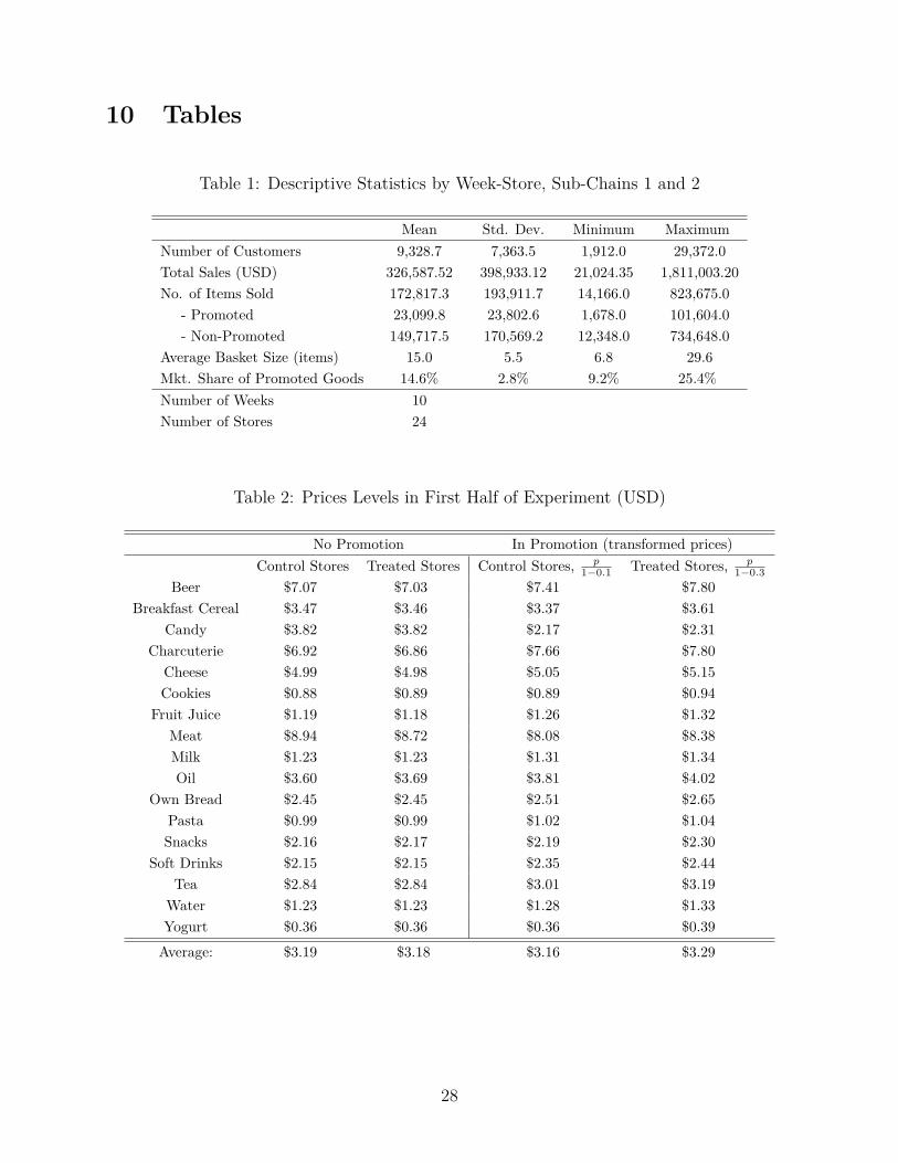
The experimental period occurred from July until September 2013. Table 1 shows thedescriptive statistics of the collected dataset per store-week pair. On average each storeserved about 3,700 customers per week and sold approximately 42,000 items.9

We inspect price levels to verify whether the experimental manipulation was correctlyimplemented. Table 2 shows the average price levels of products in the experimental set percategory, during the first half of the experiment. The first two columns show that the averagecategory prices are very similar when items are not being promoted, in accordance with theschedule in Figure 1. The third and fourth columns analyze price levels when products werebeing promoted: In order to make comparisons easier we “undo” price promotions by 10% inthe case of control stores and by 30% in the case of treated stores. If the experimental setupwas well implemented then these prices should be comparable. Indeed, we observe thatprices are relatively similar across conditions. Treated stores show slightly higher prices,which means that products may not have always been promoted at 30% levels. In this casethe experimental manipulation will be weaker, and our results will become conservative.

Table 3 shows the average category prices during the second half of the experiment, inwhich our experimental products were promoted at the 10% discount level. Both beforeand after the experiment price levels are very similar across stores for promotion and non-promotion regimes, which provides ex-post validity to the manipulation.

4 Preliminary Analysis and Matching

It is worth considering sales over time, which we plot for a few categories in Figure 3. On they axis we introduce the number of items sold per week. The x axis captures time, normalizedat the first promotion week for the good, i.e., week 0 is the week in which an item was firstpromoted. Finally, we plot sales across control and treated stores.

Treated stores show higher unit sales in week 0 than their control counterparts acrossall categories. In particular the Cheese and Milk categories show large sales increases at-tributable to the 30% discount vs. the 10% in control stores, whereas the Fruit Juice and

9An item is a physical unit of a stock keeping unit or SKU. For “bulk” purchases such as meat, forexample, items are counted according to the number of packages bought rather than to the total quantitybought, often measured in weight.

9

Water categories show relatively small effects. Given that products were promoted five weeksafter their initial promotion in most cases, the heightened promotion sensitivity hypothesiswould predict that treated stores sell more than control stores in week 5, when products arepromoted again but at the 10% level across stores. This effect may explain the difference insales across treatment and control stores in categories like Milk and Cheese in week 5. Asan example, the Fruit Juice category on the other hand shows only a very small differencebetween the sales of treated and control stores in week 5, and in the water category treatedstores sell less than their control counterparts.10 Finally, differences in sales over time andacross store groups also reveal that the environment is relatively noisy. We analyze the sam-ple data by comparing purchase-related behavior of treated and control customers during thesecond half of the experiment. During that period customers face the same promoted andnon-promoted prices. Mean differences in behavior across the control and treatment groupsare attributed to the experimental manipulation. The main regression for the analysis isgiven by

yi = α + β1Ti + β2Xi + εi (1)

where yi is the variable of interest for consumer i and Ti is an indicator function that equalsone for customers of treated stores. Variable Ti captures the event that a customer wasexposed to promotions with 30% (instead of 10%) discounts during the first half of theexperiment. The regression focuses only on the second half of the experiment to ensurethat only dynamic promotion effects are captured. We include controls Xi for precisionand robustness purposes, namely store-pair fixed effects and individual-level controls suchas customer gender, age and income levels, all in the form of indicator variables.11

Table 4 summarizes the results of regressing two of the variables of interest on the treat-ment condition, namely, the number of and the expenditure on items during their promotionweek for sub-chain 1.12 Heightened promotion sensitivity suggests that promotions shouldbe more effective in treated than in control stores in which case promoted items should sellmore in the first group of stores. The point estimate of the treatment effect in the firstcolumn of Table 4 suggests that each treated customer is on average likely to buy approx-

10The last result is likely to be due to the fact that some products were not promoted 5 weeks after theirinitial promotion, but in neighboring weeks. In particular note that treated stores sell more water in weeks4 through 8. We are currently investigating this possible cause.

11The age indicator variable is defined in spans of 20 years, and income levels represent socioeconomicgroups as coded by the retail chain.

12Similar results are observed for stores of retail chain 2.

10

imately 0.16 more promoted items during the second half of the experiment than his/hercontrol counterpart. Similarly, column 4 suggests that treatment induces a $0.24 additionalexpenditure on subsequently promoted items.13 Although the point estimates suggest thatdeep promotions may indeed increase future promotion sensitivity, hypothesis testing failsto support this claim at conventional statistical levels. To see this, consider the results incolumns 2 and 4, where standard errors are clustered at the store level. These columnsaccount for within-store error correlation across individuals. Because it is likely that cus-tomers who visit the same store have correlated observable and unobservable characteristics,our data is heteroscedastic at the observation level and ordinary least squares standard errorestimates are likely to be downward biased (see Bertrand, Duflo, and Mullainathan (2004)for an in-depth discussion). Columns 3 and 6 introduce controls Xi for precision and ro-bustness purposes. As expected, the inclusion of controls increases efficiency but statisticalsignificance is not attained.

Given that the validity of the p-values above relies on asymptotic results, it is possiblethat the lack of significance is due to the small store sample size rather than to a lack ofunderlying true experimental effects. Given this, we modify the statistical analysis in thefollowing ways: First, taking advantage of individual-level data, we perform a matching pro-cedure at the customer level. The goal of the matching procedure is to reduce the noisein the analysis by comparing individuals who are most similar in observable characteristics.The procedure is based not only on demographic variables but, importantly, also on behav-ioral data. The particular matching method is described in the next section, and has threeeffects on our working sample. First, it reduces the variance of the error term by approxi-mating the distribution of observable and unobservable factors across the two experimentalconditions. To the extent that unobservable factors are correlated with observable ones, thematching procedure reduces unobservable noise, making the analysis more efficient. Second,as described in the next section, the matching procedure focuses the analysis on a subset ofindividuals who are most “likely to find a match” in the opposite experimental condition.This phenomenon has one of two implications. If the “match likelihood” is uncorrelated withthe individual treatment effect, our results are representative and unbiased with regards tothe true “population treatment effect.” Alternatively, it is also possible that individuals who

13The symbol ‘$’ denotes the US Dollar currency, which was converted from Chilean Pe-sos according to the relation 1 Chilean Peso = 0.0016 USD as of April 30th, 2015. Source:www.bloomberg.com/markets/currencies/currency-converter.

11

are more likely to find a match in the opposite experimental condition also exhibit differenttreatment effects than the population ones. In this case the results of the analysis are validonly for a sub-sample of the data, and cannot be generalized to the overall population. It isimportant to note that although this changes the interpretation of our results, it does notaffect the validity of the inference.

It is important to note that independently of the matching procedure, standard errorsclustering is still required to take into account the fact that customers of the same storemay share individual characteristics and may be exposed to correlated unobservable shocks.Error clustering requires further attention because the validity of error clustering relies onan asymptotic result at the cluster rather than at the individual level. In order to take thefact that our sample is “small” at the cluster (store) level, we introduce a finite correction tothe standard error of the treatment effect. We implement the “cluster residual bootstrap-t”procedure as proposed by Cameron, Gelbach, and Miller (2008) to correct for downwardbias related to small samples.14 The “p-values” of the treatment effects in the subsequentanalysis are calculated through this procedure.

4.1 Matching

While in our supermarket setting performing customer-level price randomization is unfeasi-ble, it is possible to reduce the variance of the unobservable term by implementing a matchingprocedure. The goal of the matching procedure is to reduce experimental noise by matchingcustomers on observable factors. To the extent that observable factors are correlated withunobservable ones, the matching procedure can decrease the variance of the error term andprovide a more precise estimate of the treatment effect.

4.1.1 Methodology

The matching approach has a long tradition in the literature of treatment evaluation sinceRubin (1979). In our case, the main goal of the matching algorithm is to find “statisticaltwins” by use of pre-treatment data.

Finding a good set of observational pairs to balance the empirical distributions of observedcovariates in the treated and matched control groups can be very challenging in practice: The

14See Cameron and Miller (2015) and Imbens and Kolesar (2015) for relevant discussions and practicalguidance.

12

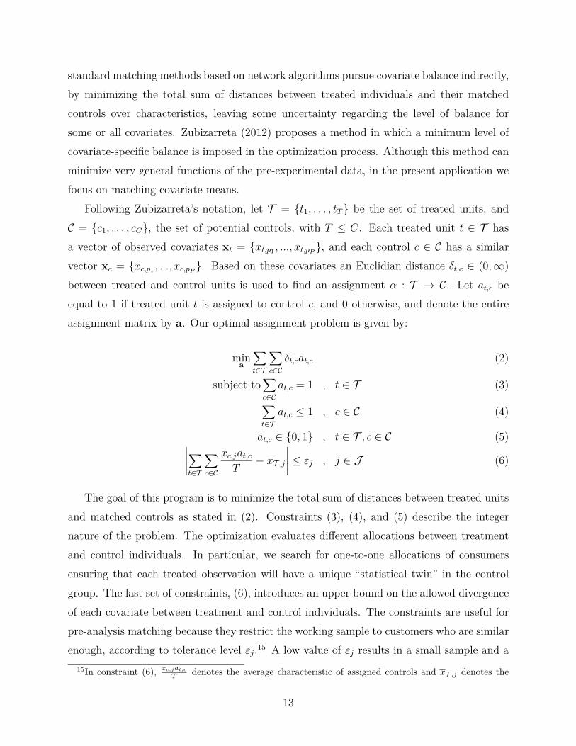
standard matching methods based on network algorithms pursue covariate balance indirectly,by minimizing the total sum of distances between treated individuals and their matchedcontrols over characteristics, leaving some uncertainty regarding the level of balance forsome or all covariates. Zubizarreta (2012) proposes a method in which a minimum level ofcovariate-specific balance is imposed in the optimization process. Although this method canminimize very general functions of the pre-experimental data, in the present application wefocus on matching covariate means.

Following Zubizarreta’s notation, let T = {t1, . . . , tT} be the set of treated units, andC = {c1, . . . , cC}, the set of potential controls, with T ≤ C. Each treated unit t ∈ T hasa vector of observed covariates xt = {xt,p1 , ..., xt,pP

}, and each control c ∈ C has a similarvector xc = {xc,p1 , ..., xc,pP

}. Based on these covariates an Euclidian distance δt,c ∈ (0,∞)between treated and control units is used to find an assignment α : T → C. Let at,c beequal to 1 if treated unit t is assigned to control c, and 0 otherwise, and denote the entireassignment matrix by a. Our optimal assignment problem is given by:

mina

∑t∈T

∑c∈C

δt,cat,c (2)

subject to∑c∈C

at,c = 1 , t ∈ T (3)∑t∈T

at,c ≤ 1 , c ∈ C (4)

at,c ∈ {0, 1} , t ∈ T , c ∈ C (5)∣∣∣∣∣∑t∈T

∑c∈C

xc,jat,c

T− xT ,j

∣∣∣∣∣ ≤ εj , j ∈ J (6)

The goal of this program is to minimize the total sum of distances between treated unitsand matched controls as stated in (2). Constraints (3), (4), and (5) describe the integernature of the problem. The optimization evaluates different allocations between treatmentand control individuals. In particular, we search for one-to-one allocations of consumersensuring that each treated observation will have a unique “statistical twin” in the controlgroup. The last set of constraints, (6), introduces an upper bound on the allowed divergenceof each covariate between treatment and control individuals. The constraints are useful forpre-analysis matching because they restrict the working sample to customers who are similarenough, according to tolerance level εj.15 A low value of εj results in a small sample and a

15In constraint (6), xc,jat,c

T denotes the average characteristic of assigned controls and xT ,j denotes the

13

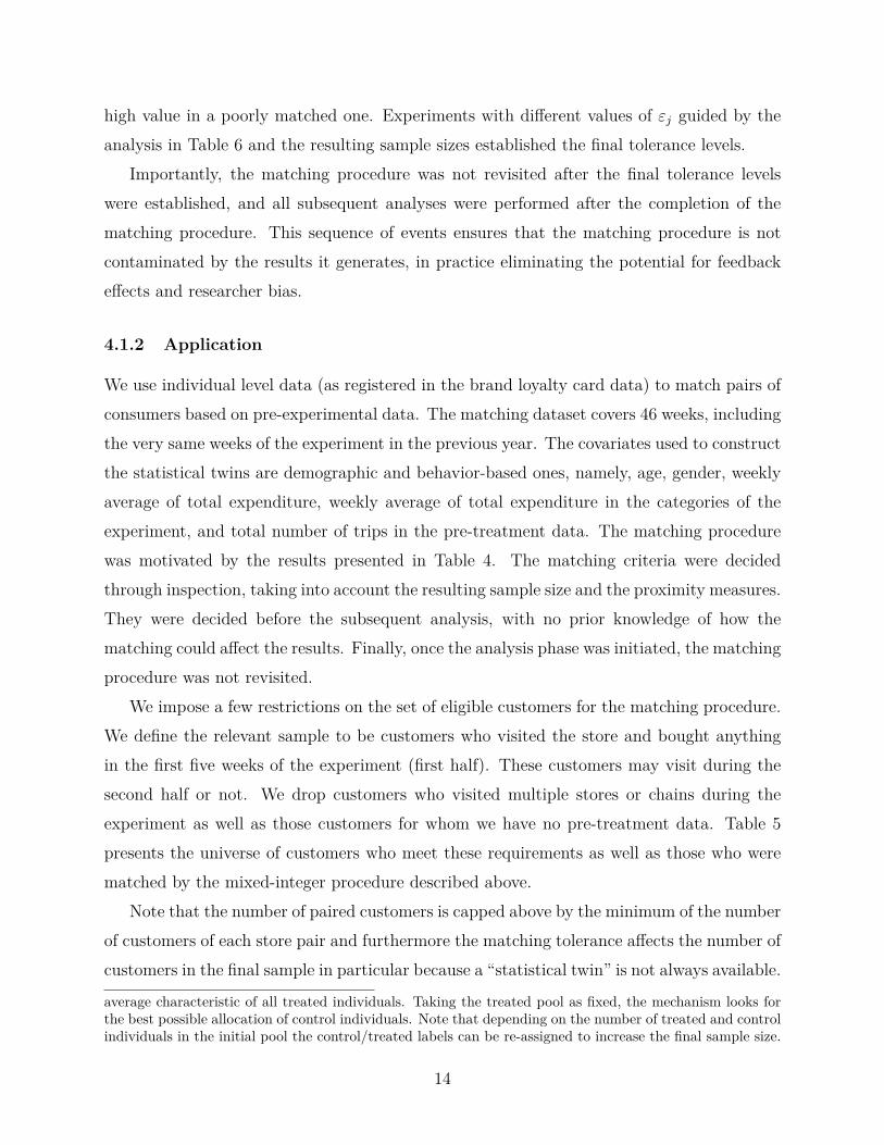
high value in a poorly matched one. Experiments with different values of εj guided by theanalysis in Table 6 and the resulting sample sizes established the final tolerance levels.

Importantly, the matching procedure was not revisited after the final tolerance levelswere established, and all subsequent analyses were performed after the completion of thematching procedure. This sequence of events ensures that the matching procedure is notcontaminated by the results it generates, in practice eliminating the potential for feedbackeffects and researcher bias.

4.1.2 Application

We use individual level data (as registered in the brand loyalty card data) to match pairs ofconsumers based on pre-experimental data. The matching dataset covers 46 weeks, includingthe very same weeks of the experiment in the previous year. The covariates used to constructthe statistical twins are demographic and behavior-based ones, namely, age, gender, weeklyaverage of total expenditure, weekly average of total expenditure in the categories of theexperiment, and total number of trips in the pre-treatment data. The matching procedurewas motivated by the results presented in Table 4. The matching criteria were decidedthrough inspection, taking into account the resulting sample size and the proximity measures.They were decided before the subsequent analysis, with no prior knowledge of how thematching could affect the results. Finally, once the analysis phase was initiated, the matchingprocedure was not revisited.

We impose a few restrictions on the set of eligible customers for the matching procedure.We define the relevant sample to be customers who visited the store and bought anythingin the first five weeks of the experiment (first half). These customers may visit during thesecond half or not. We drop customers who visited multiple stores or chains during theexperiment as well as those customers for whom we have no pre-treatment data. Table 5presents the universe of customers who meet these requirements as well as those who werematched by the mixed-integer procedure described above.

Note that the number of paired customers is capped above by the minimum of the numberof customers of each store pair and furthermore the matching tolerance affects the number ofcustomers in the final sample in particular because a “statistical twin” is not always available.

average characteristic of all treated individuals. Taking the treated pool as fixed, the mechanism looks forthe best possible allocation of control individuals. Note that depending on the number of treated and controlindividuals in the initial pool the control/treated labels can be re-assigned to increase the final sample size.

14

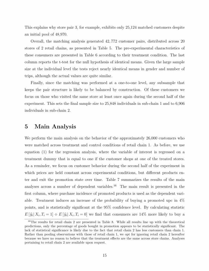
This explains why store pair 3, for example, exhibits only 25,124 matched customers despitean initial pool of 48,970.

Overall, the matching analysis generated 42, 772 customer pairs, distributed across 20stores of 2 retail chains, as presented in Table 5. The pre-experimental characteristics ofthese consumers are presented in Table 6 according to their treatment condition. The lastcolumn reports the t-test for the null hypothesis of identical means. Given the large samplesize at the individual level the tests reject nearly identical means in gender and number oftrips, although the actual values are quite similar.

Finally, since the matching was performed at a one-to-one level, any subsample thatkeeps the pair structure is likely to be balanced by construction. Of these customers wefocus on those who visited the same store at least once again during the second half of theexperiment. This sets the final sample size to 25,848 individuals in sub-chain 1 and to 6,906individuals in sub-chain 2.

5 Main Analysis

We perform the main analysis on the behavior of the approximately 26,000 customers whowere matched across treatment and control conditions of retail chain 1. As before, we useequation (1) for the regression analysis, where the variable of interest is regressed on atreatment dummy that is equal to one if the customer shops at one of the treated stores.As a reminder, we focus on customer behavior during the second half of the experiment inwhich prices are held constant across experimental conditions, but different products en-ter and exit the promotion state over time. Table 7 summarizes the results of the mainanalyses across a number of dependent variables.16 The main result is presented in thefirst column, where purchase incidence of promoted products is used as the dependent vari-able. Treatment induces an increase of the probability of buying a promoted upc in 4%points, and is statistically significant at the 95% confidence level. By calculating statisticE [ yi|Xi, Ti = 1] ÷ E [ yi|Xi, Ti = 0] we find that consumers are 14% more likely to buy a

16The results for retail chain 2 are presented in Table 8. While all results line up with the theoreticalpredictions, only the percentage of goods bought in promotion appears to be statistically significant. Thelack of statistical significance is likely due to the fact that retail chain 2 has less customers than chain 1.Rather than pooling observations with those of retail chain 1, we opt for ignoring retail chain 2 hereafterbecause we have no reason to believe that the treatment effects are the same across store chains. Analysespertaining to retail chain 2 are available upon request.

15

promoted item than their control counterparts, despite the fact that both observe the samepromotional discount.

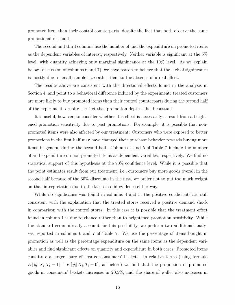
The second and third columns use the number of and the expenditure on promoted itemsas the dependent variables of interest, respectively. Neither variable is significant at the 5%level, with quantity achieving only marginal significance at the 10% level. As we explainbelow (discussion of columns 6 and 7), we have reason to believe that the lack of significanceis mostly due to small sample size rather than to the absence of a real effect.

The results above are consistent with the directional effects found in the analysis inSection 4, and point to a behavioral difference induced by the experiment: treated customersare more likely to buy promoted items than their control counterparts during the second halfof the experiment, despite the fact that promotion depth is held constant.

It is useful, however, to consider whether this effect is necessarily a result from a height-ened promotion sensitivity due to past promotions. For example, it is possible that non-promoted items were also affected by our treatment: Customers who were exposed to betterpromotions in the first half may have changed their purchase behavior towards buying moreitems in general during the second half. Columns 4 and 5 of Table 7 include the numberof and expenditure on non-promoted items as dependent variables, respectively. We find nostatistical support of this hypothesis at the 90% confidence level. While it is possible thatthe point estimates result from our treatment, i.e., customers buy more goods overall in thesecond half because of the 30% discounts in the first, we prefer not to put too much weighton that interpretation due to the lack of solid evidence either way.

While no significance was found in columns 4 and 5, the positive coefficients are stillconsistent with the explanation that the treated stores received a positive demand shockin comparison with the control stores. In this case it is possible that the treatment effectfound in column 1 is due to chance rather than to heightened promotion sensitivity. Whilethe standard errors already account for this possibility, we perform two additional analy-ses, reported in columns 6 and 7 of Table 7. We use the percentage of items bought inpromotion as well as the percentage expenditure on the same items as the dependent vari-ables and find significant effects on quantity and expenditure in both cases. Promoted itemsconstitute a larger share of treated consumers’ baskets. In relative terms (using formulaE [ yi|Xi, Ti = 1] ÷ E [ yi|Xi, Ti = 0], as before) we find that the proportion of promotedgoods in consumers’ baskets increases in 20.5%, and the share of wallet also increases in

16

16.6%. These figures suggest that the heightened promotion sensitivity caused by deeperpromotions is economically significant, and we discuss this point further in Section 7.

Taken together, the analyses above indicate that deeper promotions increase sensitivity tofuture promotions. Although both treated and control consumers face the same promotionsduring the second half of the experiment, the treated customers are most likely to buypromoted goods than their control counterparts. Moreover, they devote a significantly highershare of wallet to promoted products as well. The finding lends support to the notionthat customers become more promotion sensitive after receiving more attractive promotions.Various mechanisms, such as search behavior, stockpiling behavior and state dependence arelikely to occur in our context, and have different implications on our results. We discussmechanisms in the next Sections.

5.1 Who is Affected by Deep Discounts?

The results from the previous section suggest that deep discounts today lead to higher cus-tomers’ sensitivity to future discounts on average. An average effect, however, provides onlya summary of the effect of the treatment on different shoppers. In this section we investi-gate whether there exist individual characteristics that systematically predict how customersreact to the treatment. This analysis has a dual purpose. First, understanding which indi-vidual characteristics moderate the response to treatment is not only useful for academicsbut for practitioners as well. For example, while trying to understand consumer behaviorfirms find it useful to identify which consumer segment(s) become more promotion sensi-tive after a period of deep discounts. In this case knowledge about treatment heterogeneitymay inform the firm about the geographical locations in which to provide deep discounts,or about which subsequent marketing mixes to target different sets of consumers after pe-riods of deep discounts have occurred. Second, understanding treatment moderators alsosheds light on the mechanism underlying our treatment effect. Given the recent findingsthat behavior-based characteristics have in terms of predictive power, over and above othersrelated to demographics, we introduce two behavioral moderators, namely, the historicalaverage basket size and the propensity to buy promoted items in the past. The results ofthe treatment interactions are summarized in Table 10. The analysis includes the relevantmain effects for the interactions but we omit them in our reporting.

We find that the higher the number of items bought in promotion in the past, controlling

17

for average basket size, the more a consumer is likely to buy more promoted goods in lightof past deep promotions. These consumers are likely to buy more promoted goods duringthe second half than their control counterparts, and spend more on those items as well. Wealso find weak statistical evidence towards these consumers also buying more non-promotedgoods as well, which suggests a complementary effect of promotions on other non-promotedproducts. However, in terms of basket composition, columns 6 and 7 show that consumerswith higher propensity to buy promoted items react disproportionately towards promoteditems during the second half of the experiment. Hence, our experiment seems to “activate”deal seekers in the first place. We revisit this finding when we consider search behavior.

Basket size has no bearing on treatment effects except for the expenditure allocationacross goods. While we do not have a theory related to household size to explain this, me-chanically speaking the result shows that consumers with larger baskets shift their purchasesto cheaper promoted goods and more expensive non-promoted goods. Stockpiling behavior,in particular, may explain the result. For example, these consumers may have stocked up onpromoted goods during the first half of the experiment to a higher extent, and during thesecond half their focus is on more expensive non-promoted goods a whole.

5.2 Category-Level Effects

We first analyze the treatment effect at the category level, by regressing incidence andquantity of promoted items bought on treatment and additional controls, using the sameanalysis as before. Panel a) of Figure 4 presents the results.

We find heterogeneity in treatment effects across multiple categories. Milk, water andfruit juices show the largest effects, whereas beer, store-brand bread and cookies show nosignificant effects, although all results are directionally positive.

We use the existence of multiple categories to explore the nature of the reaction totreatment further. In particular, we ask whether a purchase in a category during the firsthalf of the experiment is necessary for deep promotions to have an effect on promotionsensitivity. Panel b) of Figure 4 shows within-category treatment effects conditional on nocategory purchases in the first half by a given individual. As in Panel a) of Figure 4, wesort categories by the magnitude of the treatment effect. Visual inspection reveals thatthe ranking does not change much once the analysis focus is only on customers who didnot purchase from a given category during the first half of the experiment. Moreover, all

18

effects are lower than the original treatment effects, and only two categories show significanttreatment results. Our explanation is that it is likely that customers who did not buy from agiven category during the first half of the experiment were still exposed to promotions acrossmultiple categories as they walked through the shopping aisles, and a higher promotionsensitivity resulted during the second half of the experiment. Based on these figures, itseems that purchasing from a particular category is not a necessary condition for heightenedpromotion sensitivity to arise from deep promotions in that particular category. The claimis that promotion depth affects future promotion sensitivity in other ways than only throughpurchase behavior. In other words, purchase behavior is not a full mediator. (See Figure 5for details.)

6 Searching for Deals

In this section we show that changes in consumer search can rationalize our experimentalfindings of treated consumers increasing the share of promoted items in their baskets. Intu-itively, deep discounts can change beliefs of the promoted price distribution increasing theexpected gains of searching promoted goods. Hence, deeper discounts in the first half caninduce more search within promoted products thus increasing the fraction of promoted itemsbought relative to no promoted ones.

6.1 Model

In order to identify a mechanism that rationalize our experimental findings, we built on thesequential search model of Weitzman (1979).

Suppose there are n items of uncertain reward or net utility. Each good i at time thas a potential reward or net utility xj

it that depends on three terms: i) a time-invariantproduct-specific utility, ui ; ii) a mean zero stochastic utility shock, εit ; and iii) the price ofthe product i at time t in status j, pj

it. The price status can be at the regular price level,denoted by pr

it; or at a lower promoted/discounted price level denoted by pdit. Consumers can

freely observe price status j = {r, d} through noticeable price tags, but they need to engagein costly search to observe price pj

it and the other components εit and ui.

19

The net utility is given by:

xjit = ui + εit − pj

it j = {r, d} (7)

The uncertain net utility of products has a probability distribution function F j, that dependson whether the product is discounted or not (j = {r, d}).

The distribution function, F j, captures the consumer beliefs regarding the distributionof net utilities of unsearched products in the store. Given the nature of frequently-purchasedproducts, we assume that consumer’s current beliefs on the gains of products in status j area function of the average of prices in status j in the last period. Formally :

F j(xjit|pj

t−1) j = {r, d} (8)

where pjt−1 is the average price in status j = {r, d} at time (t− 1) in a given store.

Consider the case in which an individual endowed with a certain value z0 is consideringwhether to inspect the value of an unsearched item, with inspection cost c > 0. Assume nodiscounting. In this case the expected value of searching the new alternative is given by:

−c+ Pr(xj

it ≥ z0|pjt−1

)E[xj

it

∣∣∣xjit ≥ z0, pj

t−1

]+ Pr

(xj

it < z0|pjt−1

)z0 (9)

It is clear that the consumer should search if the expected gains (equation 9) are larger thanz0 that is the current value of not searching.

Define the reservation value or reservation price zjit as the certain net utility that makes

the consumer indifferent between searching and not searching. The following condition forthe reservation value zj

it must hold

c =ˆ +∞

zjit

(xj

it − zjit

)dF (xj

it|pjt−1) (10)

Clearly, if z0 > zjit the individual prefers to search whereas if z0 ≤ zj

it the individual prefersto stop searching.

As an algorithmic solution to the problem with multiple different options, Weitzmanshowed the optimality of “Pandora’s rule”:

1. Selection rule: If a product is to be inspected, it should be the remaining product with

20

highest reservation price.

2. Stopping rule: Terminate search whenever the maximum sampled reward exceeds thereservation price of every non-inspected items.

Hence, the optimal search procedure implies, at each decision point, to calculate thereservation value of each unsearched option, and compare it with the value of the highestoption found until that moment. If the maximum of the reservation values of the unsearchedoptions is higher than the maximum of the utilities of searched options then the consumershould go ahead and search the most promising alternative. Otherwise, it is best to stopsearching.

A direct implication of equation (10) is that as rewards become more dispersed at theupper end of the distribution, the reservation price increases and so does the net benefit ofsearch. In Weitzman’s words:

“Other things being equal, it is optimal to sample first from distributions whichare more spread out or riskier in hopes of striking it rich early and ending thesearch. Low-probability high-payoff situations should be prime candidates forearly investigation even though they may have a smaller chance of ending up asthe source ultimately yielding the maximum reward when search ends.”

In our particular case, if the exposure to deeper promotions shifted the probability massof rewards of promoted items to the right, then the reservation price of promoted itemsare larger and thus consumers start searching over promoted items first. Our experimentdesign ensures that the average regular price is identical but promoted items exhibit a largerdiscount at treated store than control stores.

It is an empirical question whether deep discounts in past lead to more optimistic expec-tations about future prices of promoted items.

6.2 Empirical Evidence

To asses whether the search model can predict a consumer basket biased towards promoteditems, we study the transition matrix of prices using our pre-treatment data. We discretizethe space of prices into three states: regular prices (no discount), low-discount promotion

21

(discounts between 0 and 20 percent), and high-discount promotion (discounts above 20percent).

Table 11 presents the transition matrix of prices conditional on prices being in low dis-count promotions in the last period (discounts of 20 percent or less). For instance, if Oilprices exhibited a 10 percent discount in the last period, the probability of the oil prices to beat their regular price is 64 percent, whereas the probability of remaining at the low-discountlevel is 36 percent. Importantly, the probability of oil price changing to a deeper level ofdiscount is zero.

Similarly, Table 12 presents the transition matrix of prices conditional on prices in thehigh-discount state last period. The results are similar in the sense that the probabilities ofreturning to regular prices are high (75 percent) on average, and that the probabilities ofprices remaining in the same level of discount are 25 percent on average. Importantly, con-ditional on prices being in the high-discount state last period, the probabilities of observingthe low-discount prices are zero.

Therefore, the general finding is that prices at a given level of discount tend to returnto regular prices or to stay in their current level of discounts. The probabilities of switchingbetween the high-discount level and the low-discount level are zero for every single categoryof our experiment.

Based on tables 11 and 12, the consumers in the control stores were expecting low-discount prices or regular prices. Instead , the consumers in the treated stores were expectinghigh-discount promotions or regular prices. That is exactly the scenario were the exposureto deeper promotions shifted the probability mass of rewards of promoted items to the right,and therefore the reservation price of promoted items are larger in treated stores and thustreated consumers are more likely to start searching over promoted items first. Hence, wefind empirical support to the hypothesis that a search model can rationalize the expenditurebeing biased towards promoted items after the high-discount period.

7 Effects for Competing Firms (Work in Progress)

We now investigate the economic significance of the results above in terms of their effectson brands. Because manufacturers engage in competition, a change in promotion sensitivityyields both direct and strategic effects. In order to capture both we introduce a demand

22

and supply model to leverage the experimental variation and assess the short run influenceof heightened promotion sensitivity.

Let customer i derive utility from purchasing good j on week t according to

uijt = αj + β1dijt−1 + β2ipijt + εijt (11)

= vijt + εijt (12)

where αj is a common utility value of product j across consumers, dijt−1 denotes statedependence, which is equal to one if customer i bought product j in the previous categorypurchase, and pijt is the price of product j customer i faces at time t.17 In addition, customeri receives utility from an outside option according to ui0t = εi0t if she visits the store butdoes not buy from the focal category. Hence, we analyze behavior conditional on a storevisit.

It is important to stress that pijt is the level of the discounted price rather than of theregular price, because by construction we observe no regular price variation in the data, andso the influence of the regular price is captured by term αj. We allow β2i to vary acrossconsumers according to

β2i = γ0 + γ1Xi + γ2Ti (13)

such that the sensitivity to the promoted price is influenced through the previous pastpromotion depth through Ti.18 Moreover, we introduce the same controls as in the mainanalysis in order to add further explanation power to reactions to promotional pricing.

By assuming εijt to be extreme value type 1 distributed, it follows that firm j’s expectedmarket share at time t is equal to

Sjt (pijt) = M−1∑i

sijt (pijt) = M−1∑i

exp (vijt)1 + exp (vijt)

(14)

where M is the number of customers in the experimental sample, equal to 25,848. Weestimate the choice model above for the second half of the experiment in the milk category.The results of interest are shown in Table 13. We find that being exposed to 30% promotions

17Subscript (t-1) in dijt−1 is imprecise in that it relates to the previous purchase in the category ratherthan to the week previous to week t.

18The existing data variation allows us to identify unobserved heterogeneity in term β2i. This expansionis currently being implemented.

23

during the first half reduces parameter β2i by 0.001 units. In order to understand the impactof this change in customers’ utilities on firm profits we solve the supply-side competitionstage where firms are allowed to set a promotional price pj to all consumers. Although ineffect promotions are managed by the retailer, they are often initiated by the brands andpassed through to the end consumers.

The supply-side model considers the optimal promotional price for each firm in twoscenarios. In the first case we set Ti = 0 to capture consumer behavior after exposure to10% promotions in the previous 5 weeks. We then set Ti = 1 to capture consumer behaviorafter exposure to 30% promotions. We optimize firms’ promotional prices in both scenariosand assess the profit impact of offering deep promotions during the previous 5 weeks.

The supply-side model captures the fact that firms’ promotion depth decisions are likelyto be interdependent, and in particular assesses the extent to which heightened sensitivityto price promotions leads to fiercer competition. While price promotions can be explainedby a series of models of competition, we opt for a simple static promotional pricing game toget a parsimonious calculation.19 Firm j’s profit is given by

πj = (pj − cj) .M.Sj (pj, p−j) (15)

and the resulting first-order conditions are given by

(pj − cj)∂Sj (pj, p−j)

∂pj

+ Sj (pj, p−j) = 0, ∀j (16)

We are interested in the difference between statistics π∗j∣∣∣T = 1 and π∗j

∣∣∣T = 0 where π∗j∣∣∣T

represents firm j’s equilibrium profit conditional on the promotion price sensitivity of itscustomers being heightened (T = 1) or not (T = 0). We assume a 30% margin based on theregular price from the data to calculate firms’ costs cj.

Table 14 shows the optimal prices for different firms in both scenarios as well as the re-sulting profits. It is clear that heightened promotion sensitivity leads to fiercer competition.While the promotional price decrease is affected by only $.01 on average, profits decrease

19See Rao (2009) for reasons behind price promotions and the corresponding models. While intuitive, theBertrand pricing game does not capture the dynamics of all explanations put forth by the price promotionliterature. Instead, it is intended as a “back of the envelope” calculation of what the average short-run effectof heightened sensitivity to price promotions may entail. Finally, the model is currently being adapted toincorporate multiple upc ownership by the parent brands.

24

approximately 6% due to increased competition. 20 As a result of facing more promotionsensitive customers firms compete more fiercely and profits decrease. A 6% reduction inprofits is a sizable effect considering that it originates from differences in customer behaviordue to past promotions. Our model suggests that more attractive promotions today heightenconsumers’ promotion sensitivity. Because of this, the model also predicts that past promo-tion activity impacts present promotion activity as well: After deep promotions firms haveto promote their products further in order to compete, in face of more promotion-sensitiveconsumers. As a result promotional prices and profits decrease.

8 Robustness

8.1 Placebo Test

In this section we introduce a falsification test designed to help assess whether our exper-imental intervention is responsible for the differences in consumer behavior across treatedand control pools. We focus the analysis on customers who did not visit the supermarketduring the first half of the experiment. Since these customers were not exposed to the dif-ferential treatment conditions, finding significant effects in this pool would call into questionthe interpretation of our findings. In order to give the best possible change of falsificationwe matched these consumers as well to decrease noise.

The results of the analysis are presented in Table 15. No significant treatment effectsare found across measures. Moreover, compared to the results of the main analysis thetreatment effects are significantly closer to zero, which further suggests that our experimentplayed little if any role on the behavior of these customers. More importantly, we do not findsupport for the idea that our treatment effects were generated by non-experimental factors,like differential demand shocks across stores, for example.

8.2 State Dependence

Because our interest lies in understanding identifying heightened promotion sensitivity, it isessential that we account for other concurrent dynamic explanations of our results. One of

20The fact that firms have an operating margin (rather than receiving their selling price as profit) dictatesthat the percent change in price does not match the percentage change in profits. We are currently in touchwith managers to assess the most appropriate margin level for several categories.

25

the most significant factors is likely to be state dependence, as operationalized by Guadagniand Little (1983) and further analyzed by Dube, Hitsch, and Rossi (2010). State dependencecan potentially explain our results, as we now illustrate. Consider a pair of similar customerswho only differ on the experimental condition they were exposed to in the first half. Assumethat the treated customer bought a promoted product because of the 30% discount, whereasthe control customer decided not to purchase it, given its lower promotional discount (10%).It is possible that during the second half of the experiment both customers visit the storeon the week that the same product is on promotion again (at the 10% level). In this casethe treated customer may be more likely to buy the product in the second half not becauseof heightened promotion sensitivity but because of state dependence triggered by the 30%discount in the first half.

We repeat the main analysis but now eliminate purchases of goods that were also boughtduring the first half of the experiment. Table 10 presents the differential effects of deep pricepromotions on subsequent sensitivity to promotions of products that were not previouslybought.

The results reveal that exposure to 30% discounts on some goods make customers morelikely to buy items on promotion later on, even if they did not buy them during the firsthalf. The absence of sign and magnitude differences with the results of Table 10 suggest thatstate dependence is not responsible for the estimated treatment effects.

8.3 Stockpiling Behavior

Our experimental design may incentivize sophisticated inventory management by customers(see Blattberg and Neslin (1993) and Mela, Jedidi, and Bowman (1998) for insightful discus-sion and analyses). For example, treated customers may take advantage of 30% discounts tostockpile on some products to a higher extent than their control counterparts. Stockpilingbehavior works counter our promotional effect since we would expect treated customers toreact less to a 10% discount during the second half of the experiment because of their largerinventories held at home. Hence, although stockpiling behavior is likely to influence ourresults, it makes the analysis conservative.

26

9 Conclusion

By use of a large scale experiment this article has shown that managers have reasons tobe worried when offering promotions. We found that deep promotions heighten customers’future promotion sensitivities. In particular, customers are 14% more likely to buy promotedgoods after being exposed to 30% promotion discounts rather than 10%. Along the samelines, we find that the proportion of promoted goods in consumers’ baskets increases in20.5%, and the share of wallet also increases in 16.6% for treated consumers relative to theircontrol group. The effect varies significantly across product categories, and does not seemto require a previous purchase to take place. Moreover, the point estimates are robust tostate dependence and are made conservative by the existence of stockpiling behavior.

We show that a model of sequential search can rationalize our findings. The underlyingmechanism is that our treatment changes the conditional price distribution of consumers,inducing treated costumers to search primarily among promoted items. Given that thepromotion depth was historically persistent over time in our retailer, it seems likely thattreated consumers were expecting better deals among promoted items in the second halfrelative to their control group, explaining our main findings.

The competition model further revealed that subsequent competition becomes more fierceafter a period of deep promotions suggesting that heightened promotion sensitivity fall intothe class of Bertrand supertraps explained by Cabral and Villas-Boas (2005), in which anapparent advantage for one firm can lead to lower profits (through fiercer competition) tocompeting firms.

27

10 Tables

Table 1: Descriptive Statistics by Week-Store, Sub-Chains 1 and 2

Mean Std. Dev. Minimum MaximumNumber of Customers 9,328.7 7,363.5 1,912.0 29,372.0Total Sales (USD) 326,587.52 398,933.12 21,024.35 1,811,003.20No. of Items Sold 172,817.3 193,911.7 14,166.0 823,675.0

- Promoted 23,099.8 23,802.6 1,678.0 101,604.0- Non-Promoted 149,717.5 170,569.2 12,348.0 734,648.0

Average Basket Size (items) 15.0 5.5 6.8 29.6Mkt. Share of Promoted Goods 14.6% 2.8% 9.2% 25.4%Number of Weeks 10Number of Stores 24

Table 2: Prices Levels in First Half of Experiment (USD)

No Promotion In Promotion (transformed prices)Control Stores Treated Stores Control Stores, p

1−0.1 Treated Stores, p1−0.3

Beer $7.07 $7.03 $7.41 $7.80Breakfast Cereal $3.47 $3.46 $3.37 $3.61

Candy $3.82 $3.82 $2.17 $2.31Charcuterie $6.92 $6.86 $7.66 $7.80

Cheese $4.99 $4.98 $5.05 $5.15Cookies $0.88 $0.89 $0.89 $0.94

Fruit Juice $1.19 $1.18 $1.26 $1.32Meat $8.94 $8.72 $8.08 $8.38Milk $1.23 $1.23 $1.31 $1.34Oil $3.60 $3.69 $3.81 $4.02

Own Bread $2.45 $2.45 $2.51 $2.65Pasta $0.99 $0.99 $1.02 $1.04Snacks $2.16 $2.17 $2.19 $2.30

Soft Drinks $2.15 $2.15 $2.35 $2.44Tea $2.84 $2.84 $3.01 $3.19

Water $1.23 $1.23 $1.28 $1.33Yogurt $0.36 $0.36 $0.36 $0.39

Average: $3.19 $3.18 $3.16 $3.29

28

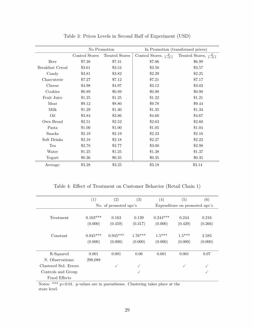
Table 3: Prices Levels in Second Half of Experiment (USD)

No Promotion In Promotion (transformed prices)Control Stores Treated Stores Control Stores, p

1−0.1 Treated Stores, p1−0.1

Beer $7.38 $7.41 $7.06 $6.99Breakfast Cereal $3.61 $3.54 $3.50 $3.57

Candy $3.81 $3.82 $2.29 $2.25Charcuterie $7.27 $7.12 $7.21 $7.17

Cheese $4.98 $4.97 $3.12 $3.02Cookies $0.89 $0.89 $0.98 $0.98

Fruit Juice $1.25 $1.25 $1.22 $1.21Meat $9.12 $8.80 $9.78 $9.44Milk $1.29 $1.30 $1.35 $1.34Oil $3.84 $3.86 $4.60 $4.67

Own Bread $2.51 $2.52 $2.63 $2.60Pasta $1.00 $1.00 $1.05 $1.04Snacks $2.19 $2.19 $2.23 $2.16

Soft Drinks $2.18 $2.18 $2.27 $2.22Tea $2.78 $2.77 $3.00 $2.98

Water $1.25 $1.25 $1.38 $1.37Yogurt $0.36 $0.35 $0.35 $0.35

Average: $3.28 $3.25 $3.18 $3.14

Table 4: Effect of Treatment on Customer Behavior (Retail Chain 1)

(1) (2) (3) (4) (5) (6)No. of promoted upc’s Expenditure on promoted upc’s

Treatment 0.163*** 0.163 0.139 0.244*** 0.244 0.216(0.000) (0.459) (0.317) (0.000) (0.429) (0.266)

Constant 0.945*** 0.945*** 1.76*** 1.5*** 1.5*** 2.583(0.000) (0.000) (0.000) (0.000) (0.000) (0.000)

R-Squared 0.001 0.001 0.06 0.001 0.001 0.07N. Observations: 298,088

Clustered Std. Errors � � � �Controls and Group

Fixed Effects� �

Notes: *** p<0.01. p-values are in parentheses. Clustering takes place at thestore level.

29

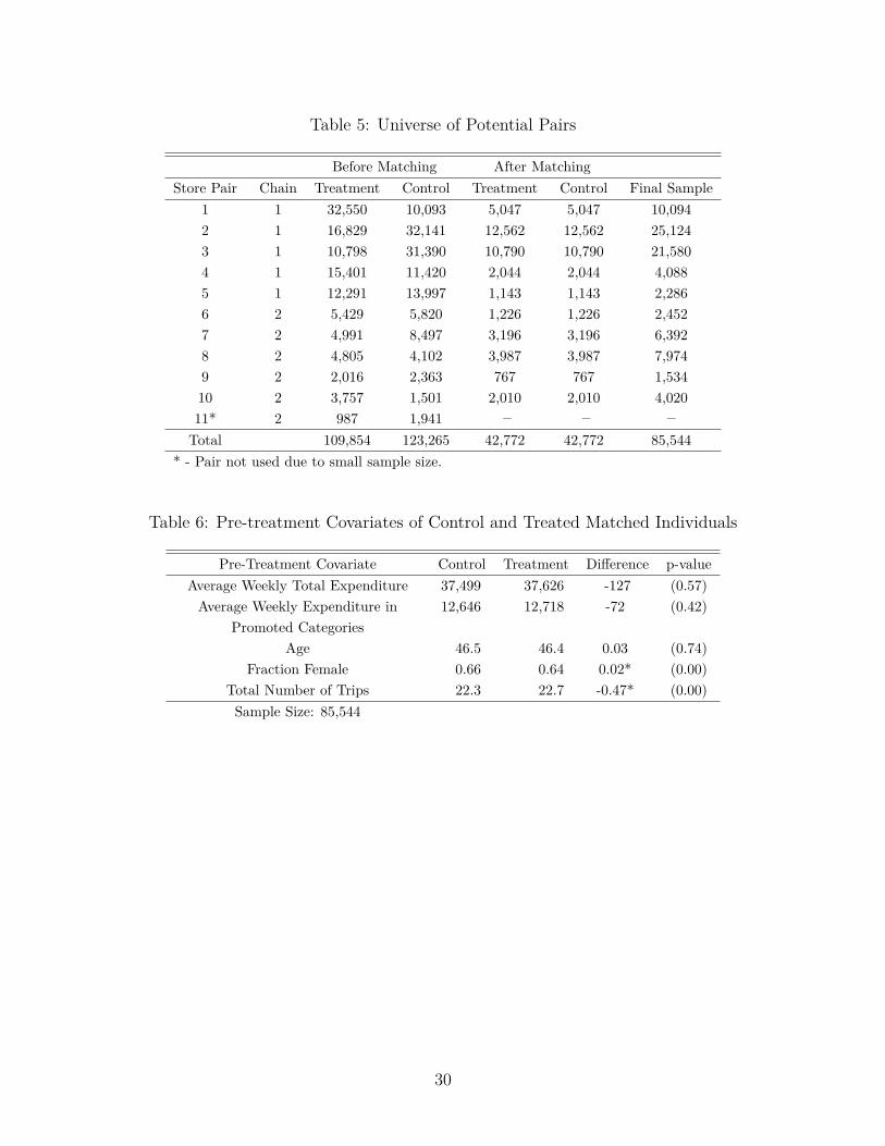
Table 5: Universe of Potential Pairs

Before Matching After MatchingStore Pair Chain Treatment Control Treatment Control Final Sample

1 1 32,550 10,093 5,047 5,047 10,0942 1 16,829 32,141 12,562 12,562 25,1243 1 10,798 31,390 10,790 10,790 21,5804 1 15,401 11,420 2,044 2,044 4,0885 1 12,291 13,997 1,143 1,143 2,2866 2 5,429 5,820 1,226 1,226 2,4527 2 4,991 8,497 3,196 3,196 6,3928 2 4,805 4,102 3,987 3,987 7,9749 2 2,016 2,363 767 767 1,53410 2 3,757 1,501 2,010 2,010 4,02011* 2 987 1,941 – – –Total 109,854 123,265 42,772 42,772 85,544

* - Pair not used due to small sample size.

Table 6: Pre-treatment Covariates of Control and Treated Matched Individuals

Pre-Treatment Covariate Control Treatment Difference p-valueAverage Weekly Total Expenditure 37,499 37,626 -127 (0.57)Average Weekly Expenditure in

Promoted Categories12,646 12,718 -72 (0.42)

Age 46.5 46.4 0.03 (0.74)Fraction Female 0.66 0.64 0.02* (0.00)

Total Number of Trips 22.3 22.7 -0.47* (0.00)Sample Size: 85,544

30

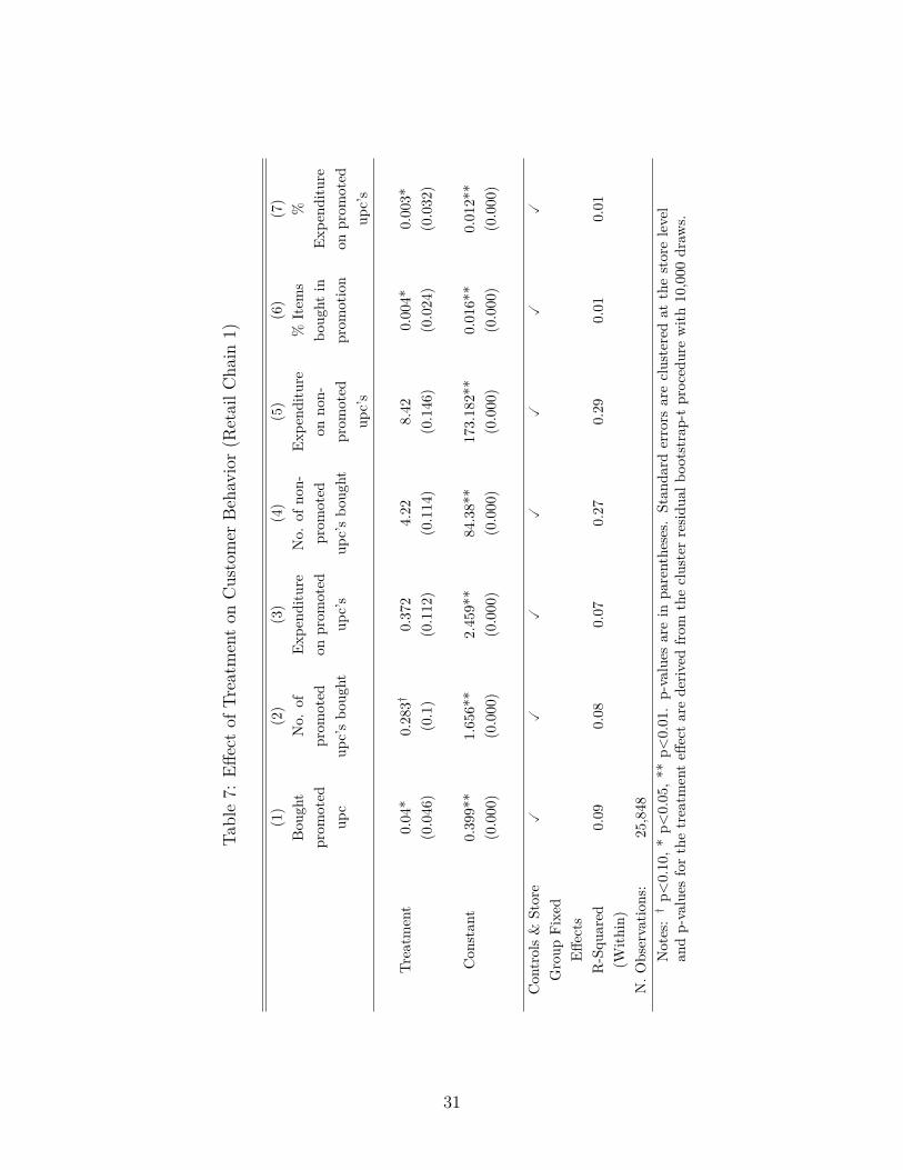
Table7:

Effectof

Treatm

enton

Customer

Beha

vior

(RetailC

hain

1)

(1)

(2)

(3)

(4)

(5)

(6)

(7)

Bou

ght

prom

oted

upc

No.

ofprom

oted

upc’sbo

ught

Expe

nditu

reon

prom

oted

upc’s

No.

ofno

n-prom

oted

upc’sbo

ught

Expe

nditu

reon

non-

prom

oted

upc’s

%Item

sbo

ught

inprom

otion

%Ex

pend

iture

onprom

oted

upc’s

Treatm

ent

0.04*

0.283†

0.372

4.22

8.42

0.004*

0.003*

(0.046)

(0.1)

(0.112)

(0.114)

(0.146)

(0.024)

(0.032)

Con

stan

t0.399**

1.656**

2.459**

84.38**

173.182**

0.016**

0.012**

(0.000)

(0.000)

(0.000)

(0.000)

(0.000)

(0.000)

(0.000)

Con

trols&

Store

Group

Fixed

Effects

��

��

��

�

R-Squ

ared

(With

in)

0.09

0.08

0.07

0.27

0.29

0.01

0.01

N.O

bservatio

ns:

25,848

Notes:†p<

0.10,*

p<0.05,*

*p<

0.01.p-values

arein

parentheses.

Stan

dard

errors

areclusteredat

thestorelevel

andp-values

forthetreatm

enteff

ectarederiv

edfrom

theclusterresid

ualb

ootstrap

-tprocedurewith

10,000

draw

s.

31

Table8:

Effectof

Treatm

enton

Customer

Beha

vior

(RetailC

hain

2)

(1)

(2)

(3)

(4)

(5)

(6)

(7)

Bou

ght

prom

oted

upc

No.

ofprom

oted

upc’sbo

ught

Expe

nditu

reon

prom

oted

upc’s

No.

ofno

n-prom

oted

upc’sbo

ught

Expe

nditu

reon

non-

prom

oted

upc’s

%Item

sbo

ught

inprom

otion

%Ex

pend

iture

onprom

oted

upc’s

Treatm

ent

0.021

0.221

0.105

1.884

3.726

0.004*

0.001

(0.243)

(0.194)

(0.401)

(0.417)

(0.315)

(0.024)

(0.563)

Con

stan

t0.42**

1.775**

1.846**

60.48**

91.73**

0.023**

0.017**

(0.000)

(0.000)

(0.000)

(0.000)

(0.000)

(0.000)

(0.000)

Con

trols&

Store

Group

Fixed

Effects

��

��

��

�

R-Squ

ared

(With

in)

0.05

0.05

0.06

0.24

0.29

0.01

0.00

N.O

bservatio

ns:

6,906

Notes:†p<

0.10,*

p<0.05,*

*p<

0.01.p-values

arein

parentheses.

Stan

dard

errors

areclusteredat

thestorelevel

andp-values

forthetreatm

enteff

ectarederiv

edfrom

theclusterresid

ualb

ootstrap

-tprocedurewith

10,000

draw

s.

32

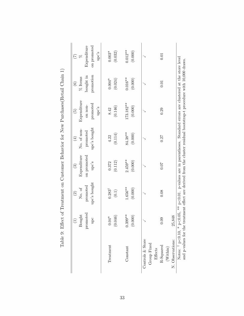
Table9:

Effectof

Treatm

enton

Customer

Beha

vior

forNew

Purcha

ses(RetailC

hain

1)

(1)

(2)

(3)

(4)

(5)

(6)

(7)

Bou

ght

prom

oted

upc

No.

ofprom

oted

upc’sbo

ught

Expe

nditu

reon

prom

oted

upc’s

No.

ofno

n-prom

oted

upc’sbo

ught

Expe

nditu

reon

non-

prom

oted

upc’s

%Item

sbo

ught

inprom

otion

%Ex

pend

iture

onprom

oted

upc’s

Treatm

ent

0.04*

0.283†

0.372

4.22

8.42

0.004*

0.003*

(0.046)

(0.1)

(0.112)

(0.114)

(0.146)

(0.024)

(0.032)

Con

stan

t0.399**

1.656**

2.459**

84.38**

173.182**

0.016**

0.012**

(0.000)

(0.000)

(0.000)

(0.000)

(0.000)

(0.000)

(0.000)

Con

trols&

Store

Group

Fixed

Effects

��

��

��

�

R-Squ

ared

(With

in)

0.09

0.08

0.07

0.27

0.29

0.01

0.01

N.O

bservatio

ns:

25,848

Notes:†p<

0.10,*

p<0.05,*

*p<

0.01.p-values

arein

parentheses.

Stan

dard

errors

areclusteredat

thestorelevel

andp-values

forthetreatm

enteff

ectarederiv

edfrom

theclusterresid

ualb

ootstrap

-tprocedurewith

10,000

draw

s.

33

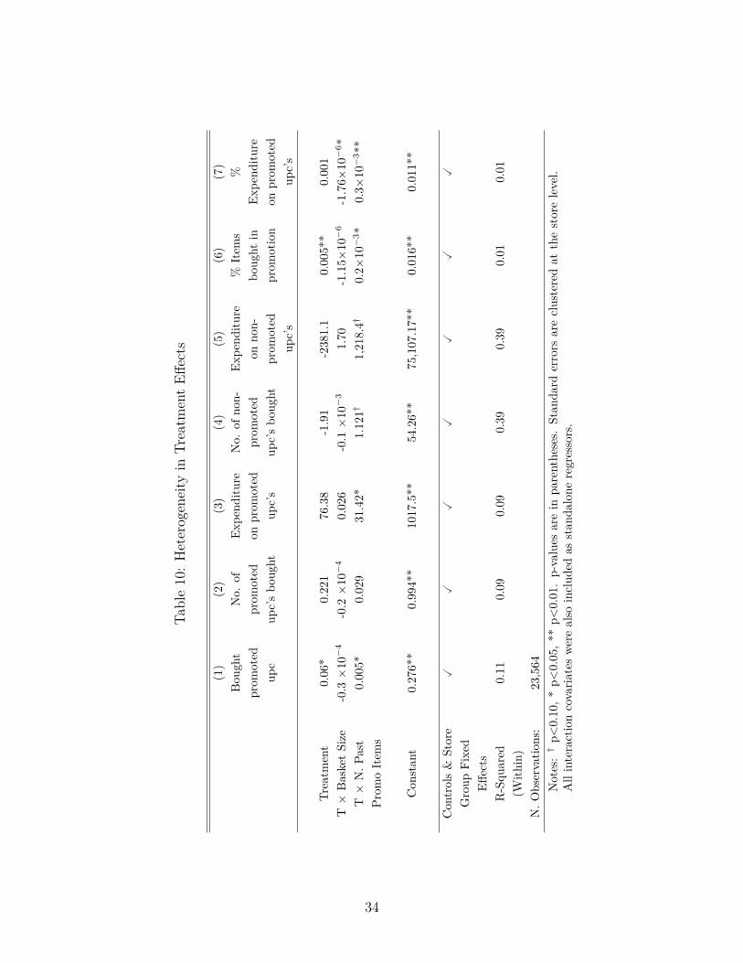
Table10:Heterogeneity

inTr

eatm

entEff

ects

(1)

(2)

(3)

(4)

(5)

(6)

(7)

Bou

ght

prom

oted

upc

No.

ofprom

oted

upc’sbo

ught

Expe

nditu

reon

prom

oted

upc’s

No.

ofno

n-prom

oted

upc’sbo

ught

Expe

nditu

reon

non-

prom

oted

upc’s

%Item

sbo

ught

inprom

otion

%Ex

pend

iture

onprom

oted

upc’s

Treatm

ent

0.06*

0.221

76.38

-1.91

-2381.1

0.005**

0.001

T×

BasketSize

-0.3×

10−

4-0.2×

10−

40.026

-0.1×

10−

31.70

-1.15×

10−

6-1.76×

10−

6 *T×

N.P

ast

Prom

oItem

s0.005*

0.029

31.42*

1.121†

1,218.4†

0.2×

10−

3 *0.3×

10−

3 **

Con

stan

t0.276**

0.994**

1017.5**

54.26**

75,107.17**

0.016**

0.011**

Con

trols&

Store

Group

Fixed

Effects

��

��

��

�

R-Squ

ared

(With

in)

0.11

0.09

0.09

0.39

0.39

0.01

0.01

N.O

bservatio

ns:

23,564

Notes:†p<

0.10,*

p<0.05,*

*p<

0.01.p-values

arein

parentheses.

Stan

dard

errors

areclusteredat

thestorelevel.

Allinteractioncovaria

teswerealso

includ

edas

stan

dalone

regressors.

34

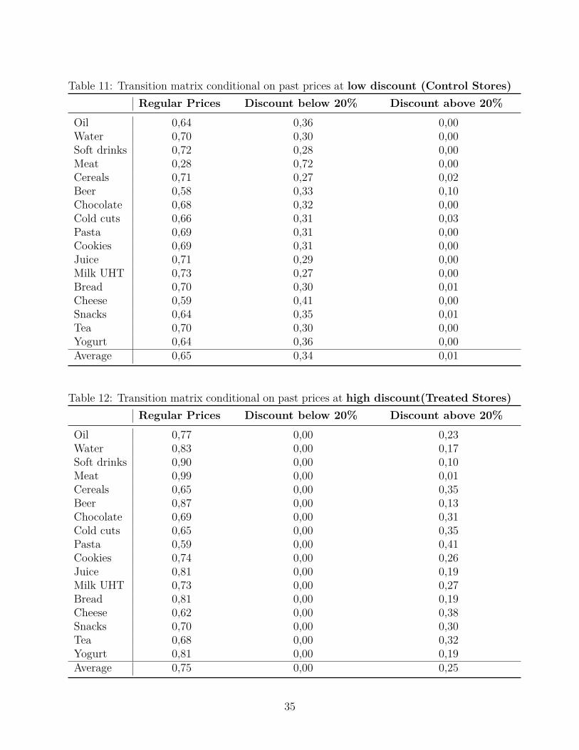
Table 11: Transition matrix conditional on past prices at low discount (Control Stores)Regular Prices Discount below 20% Discount above 20%

Oil 0,64 0,36 0,00Water 0,70 0,30 0,00Soft drinks 0,72 0,28 0,00Meat 0,28 0,72 0,00Cereals 0,71 0,27 0,02Beer 0,58 0,33 0,10Chocolate 0,68 0,32 0,00Cold cuts 0,66 0,31 0,03Pasta 0,69 0,31 0,00Cookies 0,69 0,31 0,00Juice 0,71 0,29 0,00Milk UHT 0,73 0,27 0,00Bread 0,70 0,30 0,01Cheese 0,59 0,41 0,00Snacks 0,64 0,35 0,01Tea 0,70 0,30 0,00Yogurt 0,64 0,36 0,00Average 0,65 0,34 0,01

Table 12: Transition matrix conditional on past prices at high discount(Treated Stores)Regular Prices Discount below 20% Discount above 20%

Oil 0,77 0,00 0,23Water 0,83 0,00 0,17Soft drinks 0,90 0,00 0,10Meat 0,99 0,00 0,01Cereals 0,65 0,00 0,35Beer 0,87 0,00 0,13Chocolate 0,69 0,00 0,31Cold cuts 0,65 0,00 0,35Pasta 0,59 0,00 0,41Cookies 0,74 0,00 0,26Juice 0,81 0,00 0,19Milk UHT 0,73 0,00 0,27Bread 0,81 0,00 0,19Cheese 0,62 0,00 0,38Snacks 0,70 0,00 0,30Tea 0,68 0,00 0,32Yogurt 0,81 0,00 0,19Average 0,75 0,00 0,25

35

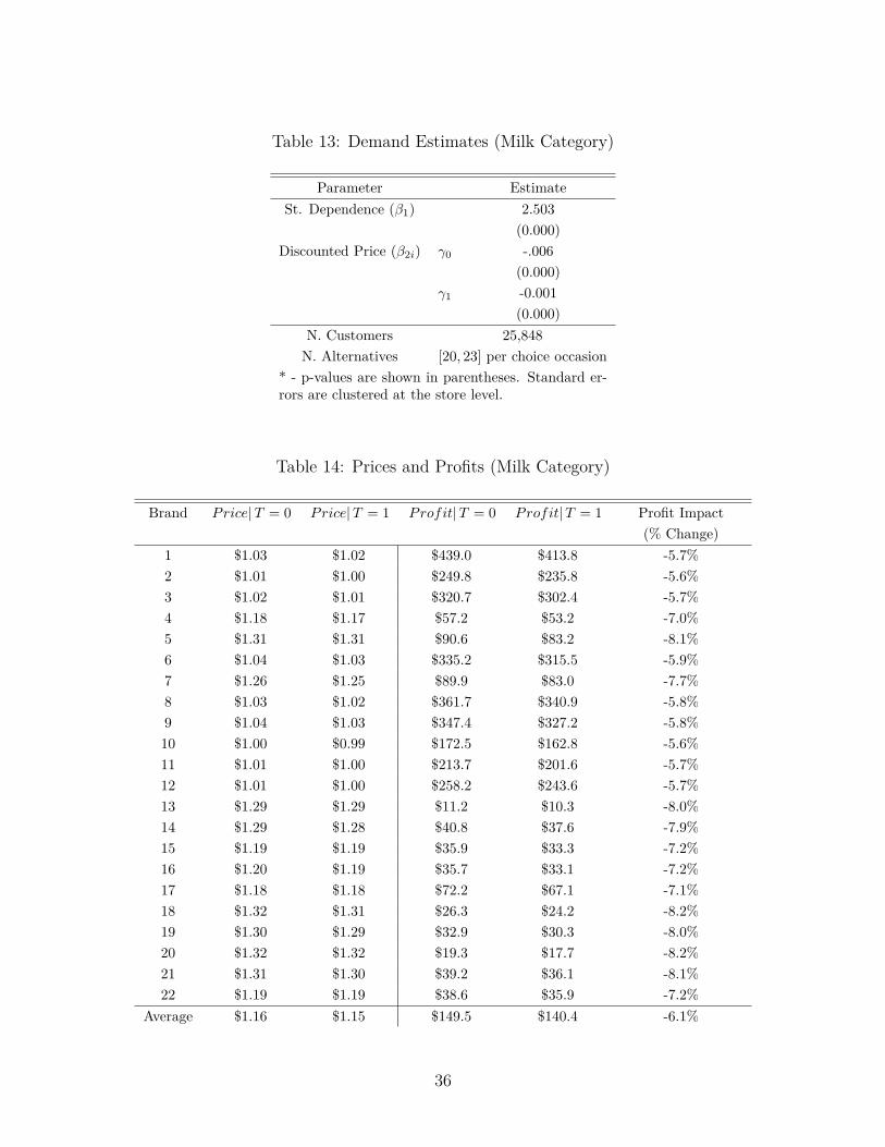
Table 13: Demand Estimates (Milk Category)

Parameter EstimateSt. Dependence (β1) 2.503

(0.000)Discounted Price (β2i) γ0 -.006

(0.000)γ1 -0.001

(0.000)N. Customers 25,848N. Alternatives [20, 23] per choice occasion

* - p-values are shown in parentheses. Standard er-rors are clustered at the store level.

Table 14: Prices and Profits (Milk Category)

Brand Price|T = 0 Price|T = 1 Profit|T = 0 Profit|T = 1 Profit Impact(% Change)

1 $1.03 $1.02 $439.0 $413.8 -5.7%2 $1.01 $1.00 $249.8 $235.8 -5.6%3 $1.02 $1.01 $320.7 $302.4 -5.7%4 $1.18 $1.17 $57.2 $53.2 -7.0%5 $1.31 $1.31 $90.6 $83.2 -8.1%6 $1.04 $1.03 $335.2 $315.5 -5.9%7 $1.26 $1.25 $89.9 $83.0 -7.7%8 $1.03 $1.02 $361.7 $340.9 -5.8%9 $1.04 $1.03 $347.4 $327.2 -5.8%10 $1.00 $0.99 $172.5 $162.8 -5.6%11 $1.01 $1.00 $213.7 $201.6 -5.7%12 $1.01 $1.00 $258.2 $243.6 -5.7%13 $1.29 $1.29 $11.2 $10.3 -8.0%14 $1.29 $1.28 $40.8 $37.6 -7.9%15 $1.19 $1.19 $35.9 $33.3 -7.2%16 $1.20 $1.19 $35.7 $33.1 -7.2%17 $1.18 $1.18 $72.2 $67.1 -7.1%18 $1.32 $1.31 $26.3 $24.2 -8.2%19 $1.30 $1.29 $32.9 $30.3 -8.0%20 $1.32 $1.32 $19.3 $17.7 -8.2%21 $1.31 $1.30 $39.2 $36.1 -8.1%22 $1.19 $1.19 $38.6 $35.9 -7.2%

Average $1.16 $1.15 $149.5 $140.4 -6.1%

36

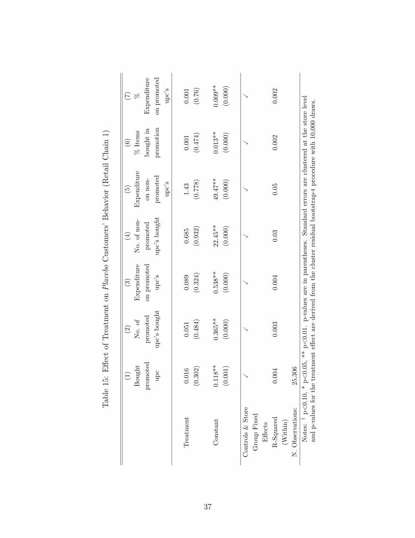
Table15:Eff

ectof

Treatm

enton

Plac

eboCustomers’

Beha

vior

(RetailC

hain

1)

(1)

(2)

(3)

(4)

(5)

(6)

(7)

Bou

ght

prom

oted

upc

No.

ofprom

oted

upc’sbo

ught

Expe

nditu

reon

prom

oted

upc’s

No.

ofno

n-prom

oted

upc’sbo

ught

Expe

nditu

reon

non-

prom

oted

upc’s

%Item

sbo

ught

inprom

otion

%Ex

pend

iture

onprom

oted

upc’s

Treatm

ent

0.016

0.051

0.089

0.685

1.43

0.001

0.001

(0.302)

(0.484)

(0.324)

(0.932)

(0.778)

(0.474)

(0.76)

Con

stan

t0.118**

0.365**

0.538**

22.45**

49.47**

0.013**

0.009**

(0.001)

(0.000)

(0.000)

(0.000)

(0.000)

(0.000)

(0.000)

Con

trols&

Store

Group

Fixed

Effects

��

��

��

�

R-Squ

ared

(With

in)

0.004

0.003

0.00

40.03

0.05

0.002

0.002

N.O

bservatio

ns:

25,306

Notes:†p<

0.10,*

p<0.05,*

*p<

0.01.p-values

arein

parentheses.

Stan

dard

errors

areclusteredat

thestorelevel

andp-values

forthetreatm

enteff

ectarederiv

edfrom

theclusterresid

ualb

ootstrap

-tprocedurewith

10,000

draw

s.

37

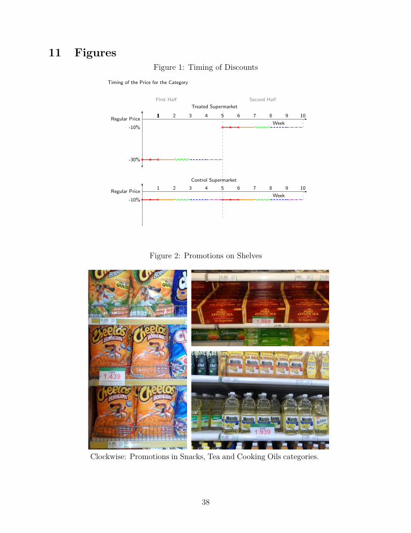
11 FiguresFigure 1: Timing of Discounts

Timing of the Price for the Category

111111 2 3 4 5 6 7 8 9 10Regular Price

-10%

-30%

Treated Supermarket

Week

1 2 3 4 5 6 7 8 9 10Regular Price

-10%

-50%

Control Supermarket

Week

First Half Second Half

Figure 2: Promotions on Shelves

Clockwise: Promotions in Snacks, Tea and Cooking Oils categories.

38

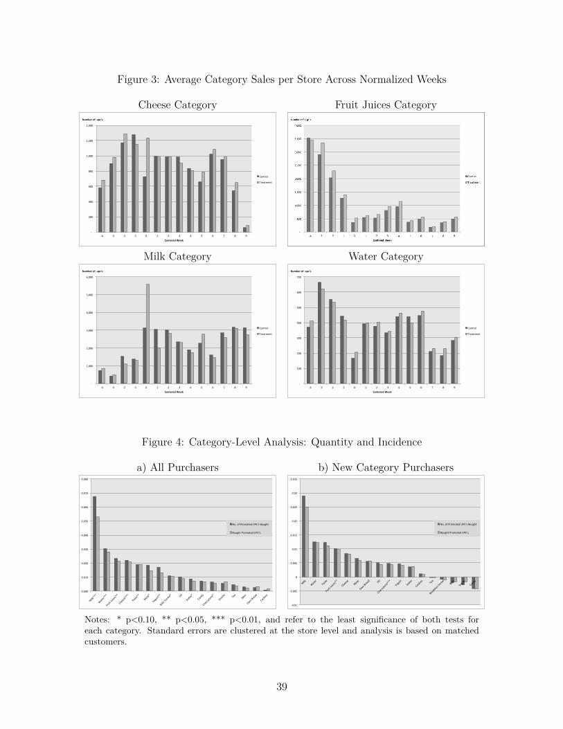
Figure 3: Average Category Sales per Store Across Normalized Weeks

Cheese Category Fruit Juices Category

 -­‐        

 200    

 400    

 600    

 800    

 1,000    

 1,200    

 1,400    

-­‐4   -­‐3   -­‐2   -­‐1   0   1   2   3   4   5   6   7   8   9  

Number  of    upc's  

Centered  Week  

Control  

Treatment  

Milk Category Water Category

 -­‐        

 1,000    

 2,000    

 3,000    

 4,000    

 5,000    

 6,000    

-­‐4   -­‐3   -­‐2   -­‐1   0   1   2   3   4   5   6   7   8   9  

Number  of    upc's  

Centered  Week  

Control  

Treatment  

 -­‐        

 100    

 200    

 300    

 400    

 500    

 600    

 700    

-­‐4   -­‐3   -­‐2   -­‐1   0   1   2   3   4   5   6   7   8   9  

Number  of    upc's  

Centered  Week  

Control  

Treatment  

Figure 4: Category-Level Analysis: Quantity and Incidence

a) All Purchasers b) New Category Purchasers

0.000  

0.010  

0.020  

0.030  

0.040  

0.050  

0.060  

0.070  

0.080  

Milk***  

Water***  

Fruit  Juices**  

Cheese***  

Pasta**  

Meat*  

Yogurt**  

Brkf.  Cereal*  

Oil  

Sodas*  

Candy  

Charcuterie*  

Snacks   Te

a  Beer  

Own  Bread  

Cookies  

No.  of  Promoted  UPC's  Bought  

Bought  Promoted  UPC's  

-­‐0.01  

-­‐0.005  

0  

0.005  

0.01  

0.015  

0.02  

0.025  

0.03  

0.035  

Milk  

Water  

Pasta  

Fruit  Juices**  

Cheese  

Meat  

Own  Bread   Oil

 

Charcuterie***  

Yogurt  

Sodas  

Cookies  

Tea  

Breakfast  Cereal  

Beer  

Snacks  

Candy  

No.  of  Promoted  UPC's  Bought  

Bought  Promoted  UPC's  

Notes: * p<0.10, ** p<0.05, *** p<0.01, and refer to the least significance of both tests foreach category. Standard errors are clustered at the store level and analysis is based on matchedcustomers.

39

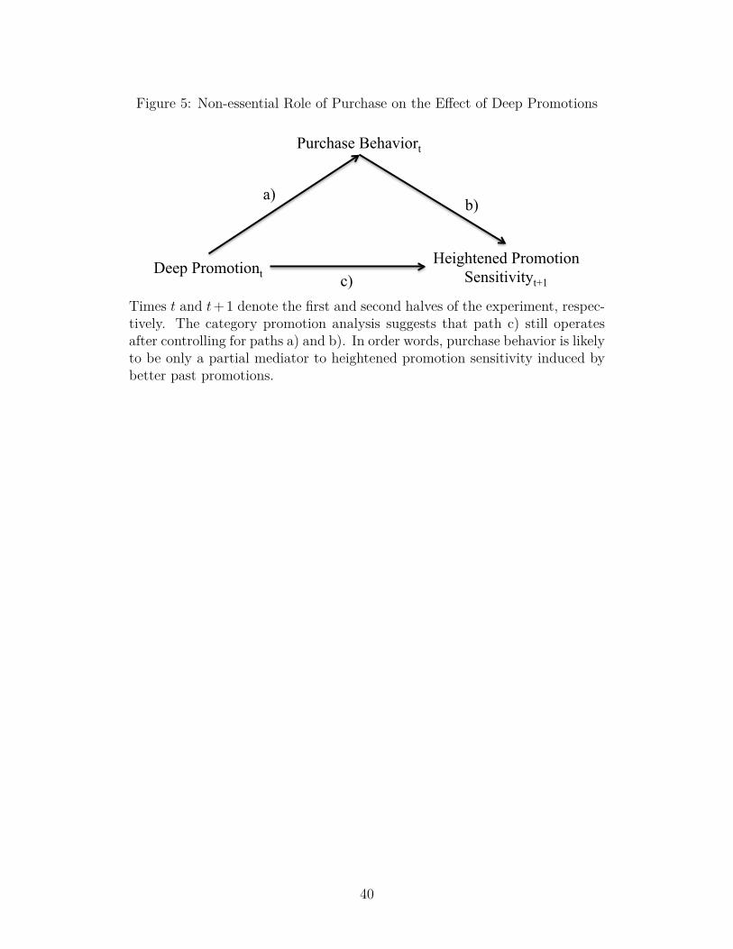
Figure 5: Non-essential Role of Purchase on the Effect of Deep Promotions

Deep Promotiont

Purchase Behaviort

Heightened Promotion Sensitivityt+1

a) b)

c) Times t and t+ 1 denote the first and second halves of the experiment, respec-tively. The category promotion analysis suggests that path c) still operatesafter controlling for paths a) and b). In order words, purchase behavior is likelyto be only a partial mediator to heightened promotion sensitivity induced bybetter past promotions.

40

ReferencesAnderson, E. T., and D. I. Simester (2004): “Long-Run Effects of Promotion Depth on New Versus

Established Customers: Three Field Studies,” Marketing Science, 23(1), 4–20.

(2010): “Price Stickiness and Customer Antagonism,” The Quarterly Journal of Economics, 125(2),729–765.

Bertrand, M., E. Duflo, and S. Mullainathan (2004): “How Much Should We Trust Differences-In-Differences Estimates?,” The Quarterly Journal of Economics, 119(1), 249–275.

Blattberg, R. C., and S. A. Neslin (1993): “Sales promotion models,” Handbooks in Operations Re-search and Management Science, 5, 553–609.

Cabral, L. M., and M. Villas-Boas (2005): “Bertrand supertraps,” Management Science, 51(4), 599–613.

Cameron, A. C., J. B. Gelbach, and D. L. Miller (2008): “Bootstrap-based improvements forinference with clustered errors,” Review of Economics and Statistics, 90(3), 414–427.

Cameron, A. C., and D. L. Miller (2015): “A practitioner’s guide to cluster-robust inference,” Journalof Human Resources, 50, 317–372.

Chan, T., C. Narasimhan, and Q. Zhang (2008): “Decomposing promotional effects with a dynamicstructural model of flexible consumption,” Journal of Marketing Research, 45(4), 487–498.

Dube, J.-P., G. J. Hitsch, and P. E. Rossi (2010): “State dependence and alternative explanations forconsumer inertia,” The RAND Journal of Economics, 41(3), 417–445.

Erdem, T., M. P. Keane, and B. Sun (2008): “A dynamic model of brand choice when price andadvertising signal product quality,” Marketing Science, 27(6), 1111–1125.

Guadagni, P. M., and J. D. Little (1983): “A logit model of brand choice calibrated on scanner data,”Marketing science, 2(3), 203–238.

Imbens, G. (2011): “Experimental Design for Unit and Cluster Randomized Trials,” 3ie, InternationalInitiative for Impact Evaluation.

Imbens, G., and M. Kolesar (2015): “Robust Standard Errors in Small Samples: Some Practical Advice,”Working Paper.

Jedidi, K., C. F. Mela, and S. Gupta (1999): “Managing advertising and promotion for long-runprofitability,” Marketing science, 18(1), 1–22.

41

Mela, C. F., S. Gupta, and D. R. Lehmann (1997): “The long-term impact of promotion and advertisingon consumer brand choice,” Journal of Marketing research, pp. 248–261.

Mela, C. F., K. Jedidi, and D. Bowman (1998): “The long-term impact of promotions on consumerstockpiling behavior,” Journal of Marketing Research, pp. 250–262.

Neslin, S. A., and H. J. Van Heerde (2008): “Promotion Dynamics,” Foundations and Trends inMarketing, 3(4).

Rao, V. R. (2009): Handbook of pricing research in marketing. Edward Elgar Publishing.

Rubin, D. B. (1979): “Using multivariate matched sampling and regression adjustment to control bias inobservational studies,” Journal of the American Statistical Association, 74(366a), 318–328.

Weitzman, M. L. (1979): “Optimal search for the best alternative,” Econometrica: Journal of the Econo-metric Society, pp. 641–654.

Zubizarreta, J. R. (2012): “Using mixed integer programming for matching in an observational study ofkidney failure after surgery,” Journal of the American Statistical Association, 107(500), 1360–1371.

42

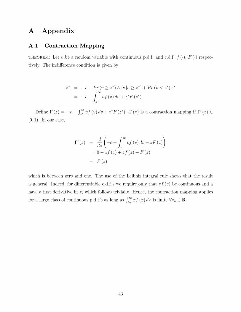
A Appendix

A.1 Contraction Mapping

theorem: Let v be a random variable with continuous p.d.f. and c.d.f. f (·), F (·) respec-tively. The indifference condition is given by

z∗ = −c+ Pr (v ≥ z∗)E [v |v ≥ z∗ ] + Pr (v < z∗) z∗

= −c+ˆ ∞

z∗vf (v) dv + z∗F (z∗)

Define Γ (z) = −c +´∞

z∗ vf (v) dv + z∗F (z∗). Γ (z) is a contraction mapping if Γ′ (z) ∈[0, 1). In our case,

Γ′ (z) = d

dz

(−c+

ˆ ∞z

vf (v) dv + zF (z))

= 0− zf (z) + zf (z) + F (z)

= F (z)

which is between zero and one. The use of the Leibniz integral rule shows that the resultis general. Indeed, for differentiable c.d.f.’s we require only that zf (v) be continuous and ahave a first derivative in z, which follows trivially. Hence, the contraction mapping appliesfor a large class of continuous p.d.f.’s as long as

´∞znxf (x) dx is finite ∀zn ∈ R.

43