Dynamic Variable Selection

with Spike-and-Slab Process Priors

Veronika Rocková & Kenichiro McAlinn

Booth School of Business, University of Chicago

January 15, 2018

Abstract

The spike-and-slab methodology for variable selection has been widely used in statisticaldata analysis since its inception more than two decades ago. However, developments for vary-ing coefficient models have not yet received much attention. Here, we address the problem ofdynamic variable selection in time series regression, where the set of active predictors is allowedto evolve over time. To capture time-varying variable selection uncertainty, we introduce newdynamic shrinkage priors for the time series of regression coefficients. These priors are char-acterized by two main ingredients: smooth parameter evolutions and intermittent zeroes formodeling predictive breaks. More formally, our proposed Dynamic Spike-and-Slab (DSS) priorsare constructed as mixtures of two processes: a spike process for the irrelevant coefficients and aslab autoregressive process for the active coefficients. The mixing weights are themselves time-varying and depend on a lagged value of the series. One distinguishing feature of DSS priors isthat their stationary distribution is fully known and characterized by spike-and-slab marginals.This property guarantees marginal stability and probabilistic coherence. We characterize dy-namic selection thresholds for MAP smoothing and implement a one-step-late EM algorithm forfast calculations. We demonstrate, through simulation and a topical high-dimensional macroe-conomic dataset, that DSS priors are far more effective at finding signal and improving forecastscompared to other existing strategies.

Keywords: Autoregressive mixture processes, Dynamic sparsity, MAP smoothing, Spike and Slab,Stationarity

1 Dynamic Sparsity

For dynamic linear modeling with many potential predictors, the assumption of a static generativemodel with a fixed subset of regressors (albeit with time-varying regressor effects) may be mis-leadingly restrictive. By obscuring variable selection uncertainty over time, confinement to a singleinferential model may lead to poorer predictive performance, especially when the actual effectivesubset at each time is sparse. The potential for dynamic model selection techniques in time seriesmodeling has been recognized (Frühwirth-Schnatter and Wagner 2010; Groen et al. 2013; Naka-jima and West 2013a; Kalli and Griffin 2014; Chan et al. 2012). One prominent practical exampleis inflation forecasting, where large sets of predictors are available and it is expected that differentsets of predictors will predict well under different economic regimes/situations (Banbura et al.2010; Nakajima and West 2013a; Koop and Korobilis 2012; Groen et al. 2013; Koop 2013; Koro-bilis 2013; Giannone et al. 2014; Kalli and Griffin 2014; Gefang 2014; Pettenuzzo et al. 2018).For example, in recessions we might see distress related factors be effective, while having no pre-dictive power in expansions. Motivated by such contexts, we develop a new dynamic shrinkageapproach for time series models that exploits time-varying predictive subset sparsity, when it infact exists.

We present our approach in the context of dynamic linear models (West and Harrison 1997)(or varying coefficient models with a time effect modifier (Hastie and Tibshirani 1993)) that link ascalar response yt at time t to a set of p known regressors xt = (xt1, . . . , xtp)

′ through the relation

yt = x′tβ0t + εt, t = 1, . . . , T, (1.1)

where β0t = (β0

t1, . . . , β0tp)′ is a time-varying vector of regression coefficients and where the inno-

vations εt come from N (0, 1). The challenge of estimating the T × p coefficients in (1.1), withmerely T observations, is typically made feasible with a smoothness inducing state-space modelthat treats {β0

t}Tt=1 as realizations from a (vector autoregressive) stochastic process

β0t = f(β0

t−1) + et, et ∼ N (0,Λt) (1.2)

for some Λt and f(·). Nevertheless, any regression model with a large number of potential pre-dictors will still be vulnerable to overfitting. This phenomenon is perhaps even more pronouncedhere, where the regression coefficients are forced to be dynamically intertwined. The major con-cern is that overfitted coefficient evolutions disguise true underlying dynamics and provide mis-leading representations with poor out-of-sample predictive performance. For long term forecasts,this concern is exacerbated by the proliferation of the state space in (1.2). As the model propagatesforward, the non-sparse state innovation accumulates noise, further hindering the out-of-sampleforecast ability. With many potentially irrelevant predictors, seeking sparsity is a natural remedyagainst the loss of statistical efficiency and forecast ability.

We shall assume that p is potentially very large, where possibly only a small portion of predic-tors is relevant for the outcome at any given time. Besides time-varying regressor effects, we adoptthe point of view that the regressors are allowed to enter and leave the model as time progresses,rendering the subset selection problem ultimately dynamic. This anticipation can be reflected bythe following sparsity manifestations in the matrix of regression coefficientsB0

p×T = [β01, . . . ,β

0T ]:

(a) horizontal sparsity, where each individual time series {β0tj}Tt=1 (for j = 1, . . . , p) allows for

1

intermittent zeroes for when jth predictor is not a persisting predictor at all times, (b) verticalsparsity, where only a subset of coefficients β0

t = (β0t1, . . . , β

0tp)′ (for t = 1, . . . , T ) will be active at

the tth snapshot in time.This problem has been addressed in the literature by multiple authors including, for example,

Groen et al. (2013); Belmonte et al. (2014); Koop and Korobilis (2012); Kalli and Griffin (2014);Nakajima and West (2013a). We should like to draw particular attention to the latent thresholdprocess of Nakajima and West (2013a,b); Zhou et al. (2014); Nakajima and West (2015, 2017),a related regime switching scheme for either shrinking coefficients exactly to zero or for leavingthem alone on their autoregressive path:

βtj = btjγtj , where γtj = I(|btj | > dj), (1.3)

btj = φ0j + φ1j(bt−1j − φ0j) + et, |φ1j | < 1, etiid∼ N (0, λ1). (1.4)

The model assumes a latent autoregressive process {btj}Tt=1, giving rise to the actual coefficients{βtj}Tt=1 only when it meanders away from a latent basin around zero [−dj , dj ]. This process isreminiscent of a dynamic extension of point-mass mixture priors that exhibit exact zeros (Mitchelland Beauchamp 1988). Other related works include shrinkage approaches towards static co-efficients in time-varying models (Frühwirth-Schnatter and Wagner 2010; Bitto and Frühwirth-Schnatter 2016; Lopes et al. 2016). We approach the dynamic sparsity problem through the lensof Bayesian variable selection and develop it further for varying coefficient models. Namely, weassume the traditional spike-and-slab setup by assigning each regression coefficient βtj a mix-ture prior underpinned by a binary latent indicator γtj , which flags the coefficient as being eitheractive or inert. While static variable selection with spike-and-slab priors has received a lot of at-tention (Carlin and Chib 1995; Clyde et al. 1996; George and McCulloch 1993, 1997; Mitchelland Beauchamp 1988; Rockova and George 2014), the literature on dynamic variants is far moresparse (George et al. 2008; Frühwirth-Schnatter and Wagner 2010; Nakajima and West 2013a;Groen et al. 2013). Narrowing this gap, this work proposes several new dynamic extensions ofpopular spike-and-slab priors.

The main thrust of this work is to introduce Dynamic Spike-and-Slab (DSS) priors, a newclass of time series priors, which induce either smoothness or shrinkage towards zero. Theseprocesses are formed as mixtures of two stationary time series: one for the active and anotherfor the negligible coefficients. The DSS priors pertain closely to the broader framework of mix-ture autoregressive (MAR) processes with a given lag, where the mixing weights are allowed todepend on time. Despite the reported success of MAR processes (and variants thereof) for mod-eling non-linear time series (Wong and Li 2000, 2001; Kalliovirta et al. 2015; Wood et al. 2011),their potential as dynamic sparsity inducing priors has been unexplored. Here, we harvest thispotential within a dynamic variable selection framework. One feature of DSS priors, that sets itapart from the latent threshold model, is that it yields benchmark continuous spike-and-slab pri-ors (such as the Spike-and-Slab LASSO of Rockova (2017)) as its marginal stationary distribution.This property guarantees marginal stability in the selection/shrinkage dynamics and probabilisticcoherence.

By turning our time-domain priors into penalty constructs, we formalize the notion of prospec-tive and retrospective shrinkage through doubly adaptive shrinkage terms that pull together past,current, and future information. We introduce asymmetric dynamic thresholding rules –extensionsof existing rules for static symmetric regularizers (Fan and Li 2001; Antoniadis and Fan 2001)–

2

to characterize the behavior of joint posterior modes for MAP smoothing. For calculation, we im-plement a one-step-late EM algorithm of (Green 1990), that capitalizes on fast closed-form one-site updates. Our dynamic penalties can be regarded as natural extensions of the spike-and-slabpenalty functions introduced by Rockova (2017) and further developed by Rockova and George(2016). The DSS priors here are deployed as a fast MAP smoothing catalyst rather than a vehiclefor a full-blown MCMC analysis (as in Nakajima and West (2013a)). The key distinguishing fea-ture of this deployment is that DSS priors attain sparsity through sparse posterior modes ratherthan auxiliary thresholding. In addition, we derive MCMC algorithms forDSS priors that leverageconditional conjugacy for forward filtering and backward sampling (Appendix).

We demonstrate the effectiveness of our introduced DSS priors with a thorough simulationstudy and a topical macroeconomic application. Both studies highlight the comparative improve-ments –in terms of inference, forecasting, and computational time– of DSS priors over conven-tional and recent methods in the literature. In particular, the macroeconomic application, using alarge number of economic indicators to forecast inflation and infer on underlying economic struc-tures, serves as a motivating example as to why dynamic sparsity is effective, and even necessary,in these contexts.

The paper is structured as follows: Section 2 and Section 2.1 introduce the DSS processes andtheir variants. Section 3 develops the penalized likelihood perspective, introducing the prospec-tive and retrospective shrinkage terms. Section 4 provides useful characterizations of the globalposterior mode. Section 5 develops the one-step-late EM algorithm for MAP smoothing. Section6 illustrates the MAP smoothing deployment of DSS on simulated examples and Section 7 on amacroeconomic dataset. Section 8 concludes with a discussion.

2 Dynamic Spike-and-Slab Priors

In this section, we introduce the class of Dynamic Spike-and-Slab (DSS) priors that constitute acoherent extension of benchmark spike-and-slab priors for dynamic selection/shrinkage. We willassume that the p time series {βtj}Tt=1 (for j = 1, . . . , p) in (1.1) follow independent and identicalDSS priors and thereby we suppress the subscript j (for notational simplicity).

We start with a conditional specification of the DSS prior. Given a binary indicator γt ∈ {0, 1},which encodes the spike/slab membership at time t, and a lagged value βt−1, we assume that βtarises from a mixture of the form

π(βt | γt, βt−1) = (1− γt)ψ0(βt | λ0) + γtψ1 (βt |µt, λ1) , (2.5)

whereµt = φ0 + φ1(βt−1 − φ0) with |φ1| < 1 (2.6)

andP(γt = 1 | βt−1) = θt. (2.7)

For Bayesian variable selection, it has been customary to specify a zero-mean spike density ψ0(β |λ0),such that it concentrates at (or in a narrow vicinity of) zero. Regarding the slab distributionψ1(βt | µt, λ1), we require that it be moderately peaked around its mean µt, where the amountof spread is regulated by a concentration parameter λ1 > 0. The conditional DSS prior formu-lation (2.5) generalizes existing continuous spike-and-slab priors (George and McCulloch 1993;

3

Ishwaran and Rao 2005; Rockova 2017) in two important ways. First, rather than centering theslab around zero, the DSS prior anchors it around an actual model for the time-varying meanµt. The non-central mean is defined as an autoregressive lag polynomial of the first order withhyper-parameters (φ0, φ1). While our framework can be extended to higher-order autoregressivepolynomials where µt may also depend on values older than βt−1, we outline our method for thefirst-order autoregression due to its relative simplicity and ubiquity in practice (Tibshirani et al.2005; West and Harrison 1997; Prado and West 2010). Throughout the manuscript, however, weremark on how to suitably modify our framework for higher orders. Although estimable (subjectto stationary restrictions), (φ0, φ1) will be treated as fixed. Assuming a fixed φ1 is not too far fromthe common practice in the Bayesian literature (Omori et al. 2007; Nakajima and West 2013a, toname a few) which consists of imposing a tight prior around, but below, 1 for φ1, to ensure stable,stationary estimation. We discuss extensions of our framework for random (φ0, φ1) in Section 8.

It is illuminating to view the conditional prior (2.5) as a “multiple shrinkage" prior (George1986b,a) with two shrinkage targets: (1) zero (for the gravitational pull of the spike), and (2) µt(for the gravitational pull of the slab). It is also worthwhile to emphasize that the spike distributionψ0(βt | λ0) does not depend on βt−1, only the slab does. The DSS formulation thus inducesseparation of regression coefficients into two groups, where only the active ones are assumed towalk on an autoregressive path.

The second important generalization is implicitly hidden in the hierarchical formulation of themixing weights θt in (2.7), which casts them as a smoothly evolving process (as will be seen inSection 2.2 below). Before turning to this formulation, we discuss several special cases of DSSpriors.

2.1 Spike and Slab Pairings

Our recommended choice of the spike distribution is the Laplace density ψ0(β | λ0) = λ0

2 e−|β|λ0

(with a relatively large penalty parameter λ0 > 0) due to its ability to threshold via sparse posteriormodes, as will be elaborated on in Section 4. Under the Laplace spike distribution, the series{βt}Tt=1 is thereby stationary, iid with a marginal density ψ0(β | λ0). Another natural choice, aGaussian spike, would impose no new computational challenges due to its conditional conjugacy.However, additional thresholding would be required to obtain a sparse representation.

Regarding the slab distribution, we will focus primarily on the Gaussian slab ψ1(βt | µt, λ1)

(with mean µt and variance λ1) due to its ability to smooth over past/future values. Under theGaussian slab distribution, {βt}Tt=1 follow a stationary Gaussian AR(1) process

βt = φ0 + φ1(βt−1 − φ0) + et, |φ1| < 1, etiid∼ N (0, λ1) , (2.8)

whose stationary distribution is characterized by univariate marginals

ψST1 (βt | λ1, φ0, φ1) ≡ ψ1

(βt

∣∣∣φ0, λ11− φ21

); (2.9)

a Gaussian density with mean φ0 and variance λ1

1−φ21. The availability of this tractable stationary

distribution (2.9) is another appeal of the conditional Gaussian slab distribution.Rather than shrinking to the vicinity of the past value, one might like to entertain the possibility

of shrinking exactly to the past value (Tibshirani et al. 2005). Such a property would be appre-

4

ciated, for instance, in dynamic sparse portfolio allocation models to mitigate transaction costsassociated with negligible shifts in the portfolio weights (Irie and West 2016; Brodie et al. 2009;Jagannathan and Ma 2003; Puelz et al. 2016). One way of attaining the desired effect would bereplacing the Gaussian slab ψ1(·) in (2.5) with a Laplace distribution centered at µt. This condi-tional construction, however, does not imply the Laplace distribution marginally. The univariatemarginals are defined through the characteristic function given in (2.7) of Andel (1983). Thelack of availability of the marginal density in a simple form thwarts the specification of transitionweights needed for the implementation of our DSS framework. There are, however, avenues forconstructing an autoregressive process with Laplace marginals, e.g., through the normal-gamma-autoregressive (NGAR) process by Kalli and Griffin (2014). We define the following Laplaceautoregressive (LAR) process as a special case.

Definition 1. We define the Laplace autoregressive (LAR) process by

βt =

√ψtψt−1

φ1βt−1 + ηt, ηt ∼ N(0, (1− φ21)ψt

),

where {ψt}Tt=1 follow an exponential autoregressive process specified through ψt |κt−1 ∼ Gamma(1+

κt−1, λ21/[2(1−ρ)]) and κt−1 |ψt−1 ∼ Poisson

(ρ

2(1−ρ)λ21ψt−1

)with a marginal distributionExp(λ21/2).

The LAR process exploits the scale-normal-mixture representation of the Laplace distribution,yielding Laplace marginals βt ∼ ψST (βt | λ1) ≡ Laplace(λ1). This coherence property can beleveraged within our DSS framework as follows. If we replace the slab Gaussian AR(1) processin (2.5) with the LAR process and deploy ψST (βt |λ1) instead of ψST (βt |λ1) in (2.11), we obtaina Laplace DSS variant with the Spike-and-Slab LASSO prior of Rockova (2017) as its marginaldistribution (according to Theorem 1).

It is worth pointing out an alternative autoregressive construction with Laplace marginals pro-posed by Andel (1983), where the following AR(1) scheme is considered.

βt =

φ1βt−1 with probability φ21,

φ1βt−1 + ηt with probability 1− φ21, where ηt ∼ Laplace(λ1).(2.10)

The innovations in (2.10) come from a mixture of a point mass at zero, providing an opportunityto settle at the previous value, and a Laplace distribution. Again, by deploying this process in theslab, we obtain the Spike-and-Slab LASSO marginal distribution. While MCMC implementationscan be obtained for the dynamic Spike-and-Slab LASSO method (e.g. embedding the sampler ofKalli and Griffin (2014) within our MCMC approach outlined in the Appendix), the Laplace slabextensions are ultimately more challenging for optimization. Throughout the rest of the paper, wethereby focus on the Gaussian AR(1) slab process.

2.2 Evolving Inclusion Probabilities

A very appealing feature of DSS priors that makes them suitable for dynamic subset selection isthe opportunity they afford for obtaining “smooth" spike/slab memberships. Recall that the binaryindicators in (2.7) determine which of the spike or slab regimes is switched on at time t, whereP(γt = 1 |βt−1) = θt. It is desirable that the sequence of slab probabilities {θt}Tt=1 evolves smoothlyover time, allowing for changes in variable importance as time progresses and, at the same time,

5

avoiding erratic regime switching. Because the series {θt}Tt=1 is a key driver of the sparsity pattern,it is important that it be (marginally) stable and that it reflects all relevant information, includingnot only the previous value θt−1, but also the previous value βt−1. Many possible constructions ofθt could be considered. We turn to the implied stationary distribution as a guide for a principledconstruction of θt.

For our formulation, we introduce a marginal importance weight 0 < Θ < 1, a scalar pa-rameter which controls the overall balance between the spike and the slab distributions. Given(Θ, λ0, λ1, φ0, φ1), the conditional inclusion probability θt (or a transition function θ(βt−1)) is de-fined as

θt ≡ θ(βt−1) =ΘψST1 (βt−1|λ1, φ0, φ1)

ΘψST1 (βt−1|λ1, φ0, φ1) + (1−Θ)ψ0 (βt−1|λ0). (2.11)

The conditional mixing weight θt can be interpreted as the posterior probability of classifyingthe past coefficient βt−1 as arriving from the stationary slab distribution as opposed to the (station-ary) spike distribution. This interpretation reveals how the weights {θt}Tt=1 proliferate parsimonythroughout the process {βt}Tt=1. Suppose that the past value |βt−1| was large, then θ(βt−1) willbe close to one, signaling that the current observation βt is more likely to be in the slab. Thecontrary occurs when |βt−1| is small, where βt will be discouraged from the slab because the in-clusion weight θ(βt−1) will be small (close to zero). Let us also note that the weights in (2.11)are different from the conditional probabilities for classifying βt−1 as arising from the conditionalslab in (2.5). These weights will be introduced later in Section 3.

It is tempting to regard Θ as the marginal proportion of nonzero coefficients. However, such aninterpretation is misleading because, sparsity levels are ultimately determined by the θt sequence,which is influenced by the component stationary distributions ψ0(·) and ψST1 (·), in particular bythe amount of their overlap around zero. Such an interpretation is thus inapplicable for thecontinuous spike-and-slab mixtures considered here, where more caution is needed for calibration(Rockova 2017). This issue will be revisited in Section 3.

Now that we have elaborated on all the layers of the hierarchical model, we are ready toformally define the Dynamic Spike-and-Slab Process.

Definition 2. Equations (2.5), (2.6), (2.7) and (2.11) define a Dynamic Spike-and-Slab Process(DSS) with parameters (Θ, λ0, λ1, φ0, φ1). We will write

{βt}Tt=1 ∼ DSS(Θ, λ0, λ1, φ0, φ1).

TheDSS process relates to the Gaussian mixture of autoregressive (GMAR) process of Kalliovirtaet al. (2015), which was conceived as a model for time series data with regime switches. Here, wedeploy it as a prior on time-varying regression coefficients within the spike-and-slab framework,allowing for distributions other than Gaussian. The DSS, being an instance/elaboration of theGMAR process, inherits elegant marginal characterizations (as will be seen below)

The DSS construction has a strong conceptual appeal in the sense that its marginal proba-bilistic structure is fully known. This property is rarely available with conditionally defined non-Gaussian time series models, where not much is known about the stationary distribution beyondjust the mere fact that it exists. The DSS process, on the other hand, guarantees well behavedstable marginals that can be described through benchmark spike-and-slab priors. The marginaldistribution can be used as a prior for the initial vector at time t = 0, which is typically esti-mated with the remaining coefficients. The following theorem is an elaboration of Theorem 1 of

6

Kalliovirta et al. (2015).

Theorem 1. Assume {βt}Tt=1 ∼ DSS(Θ, λ0, λ1, φ0, φ1) with |φ1| < 1. Then {βt}Tt=1 has a stationarydistribution characterized by the following univariate marginal distributions:

πST (β|Θ, λ0, λ1, φ0, φ1) = ΘψST1 (β | λ1, φ0, φ1) + (1−Θ)ψ0 (β | λ0) , (2.12)

where ψST1 (β | λ1, φ0, φ1) is the stationary slab distribution (2.9).

Proof. We assume an initial condition βt=0 ∼ πST (β0|Θ, λ0, λ1, φ0, φ1). Recall that the conditionaldensity of β1 given β0 can be written as

π(β1 | β0) = (1− θ1)ψ0(β1 | λ0) + θ1ψ1(β1 | µ1, λ1). (2.13)

From the definition of θ1 in (2.11), we can write the joint distribution as

π(β1, β0) = ΘψST1 (β0 | λ1, φ0, φ1)ψ1(β1 | µ1, λ1) + (1−Θ)ψ0 (β0 | λ0)ψ0(β1 | λ0).

Integrating π(β1, β0) with respect to β0, we obtain

π(β1) =

∫π(β1, β0)dβ0 =Θ

[∫β0

ψ1 (β1 | µ1, λ1)ψ1

(β0

∣∣∣φ0, λ11− φ21

)dβ0

]+ (1−Θ)ψ0(β1 | λ0)

=ΘψST1 (β1 | λ1, φ0, φ1) + (1−Θ)ψ0(β1 | λ0).

Theorem 1 describes the very elegant property of DSS that the univariate marginals of thismixture process are Θ-weighted mixtures of marginals. It also suggests a more general recipe formixing multiple stationary processes through the construction of mixing weights (2.11).

Remark 1. For autoregressive polynomials of a higher order h > 1, the transition weights θt could bedefined in terms of a multivariate stationary distribution evaluated at the last h values of the process,not only the last one. The marginals of such process could be then characterized in terms of a mixtureof multivariate Gaussian distributions (Theorem 1 of Kalliovirta et al. (2015)).

3 Dynamic Spike-and-Slab Penalty

Spike-and-slab priors give rise to self-adaptive penalty functions for MAP estimation, as detailedin Rockova (2017) and Rockova and George (2016). Here, we introduce elaborations for dynamicshrinkage implied by the DSS priors.

Definition 3. For a given set of parameters (Θ, λ0, λ1, φ0, φ1), we define a prospective penalty func-tion implied by (2.5) and (2.11) as follows:

pen(β | βt−1) = log [(1− θt)ψ0(β | λ0) + θt ψ1(β | µt, λ1)] . (3.14)

Similarly, we define a retrospective penalty pen(βt+1 | β) as a function of the second argument β in(3.14). The Dynamic Spike-and-Slab (DSS) penalty is then defined as

Pen(β | βt−1, βt+1) = pen(β | βt−1) + pen(βt+1 | β) + C, (3.15)

7

−0.5 0.0 0.5 1.0 1.5 2.0 2.5

−2.

0−

1.5

−1.

0−

0.5

0.0

β

Pro

spec

tive

pena

ltyProspective penalty

µt = φ1βt−1

βt−1 = 1.5λ0 = 1φ1 = 0.9λ1 = (1 − φ1

2)Θ = 0.2

(a) pen(β|βt−1 = 1.5)

0 1 2 3

−1.

0−

0.8

−0.

6−

0.4

−0.

20.

00.

2

β

Pro

spec

tive

pena

lty

Prospective penalty

µt = φ1βt−1

βt−1 = 1.5λ0 = 1φ1 = 0.9λ1 = 10(1 − φ1

2)Θ = 0.9

(b) pen(β|βt−1 = 1.5)

−0.5 0.0 0.5 1.0 1.5 2.0 2.5

−1.

2−

1.0

−0.

8−

0.6

−0.

4−

0.2

0.0

β

Pro

spec

tive

pena

lty

Prospective penalty

µt = φ1βt−1

βt−1 = 0.5λ0 = 1φ1 = 0.9λ1 = 10(1 − φ1

2)Θ = 0.9

(c) pen(β|βt−1 = 0.5)

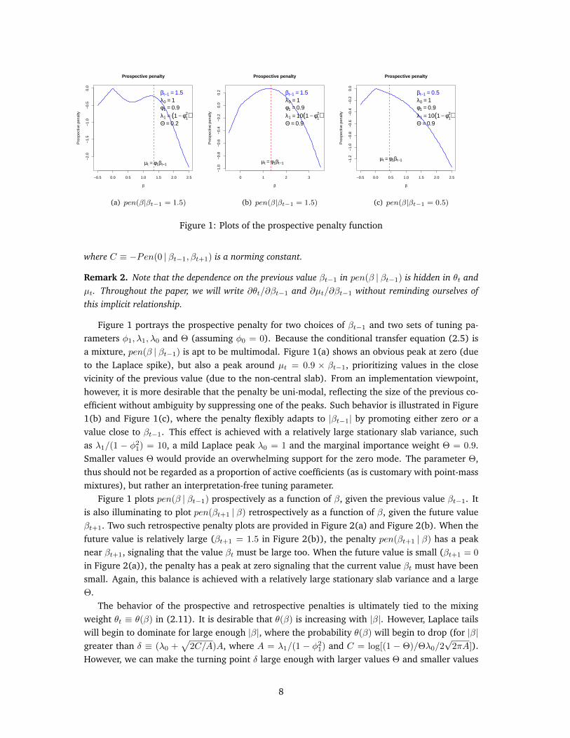
Figure 1: Plots of the prospective penalty function

where C ≡ −Pen(0 | βt−1, βt+1) is a norming constant.

Remark 2. Note that the dependence on the previous value βt−1 in pen(β | βt−1) is hidden in θt andµt. Throughout the paper, we will write ∂θt/∂βt−1 and ∂µt/∂βt−1 without reminding ourselves ofthis implicit relationship.

Figure 1 portrays the prospective penalty for two choices of βt−1 and two sets of tuning pa-rameters φ1, λ1, λ0 and Θ (assuming φ0 = 0). Because the conditional transfer equation (2.5) isa mixture, pen(β | βt−1) is apt to be multimodal. Figure 1(a) shows an obvious peak at zero (dueto the Laplace spike), but also a peak around µt = 0.9 × βt−1, prioritizing values in the closevicinity of the previous value (due to the non-central slab). From an implementation viewpoint,however, it is more desirable that the penalty be uni-modal, reflecting the size of the previous co-efficient without ambiguity by suppressing one of the peaks. Such behavior is illustrated in Figure1(b) and Figure 1(c), where the penalty flexibly adapts to |βt−1| by promoting either zero or avalue close to βt−1. This effect is achieved with a relatively large stationary slab variance, suchas λ1/(1 − φ21) = 10, a mild Laplace peak λ0 = 1 and the marginal importance weight Θ = 0.9.Smaller values Θ would provide an overwhelming support for the zero mode. The parameter Θ,thus should not be regarded as a proportion of active coefficients (as is customary with point-massmixtures), but rather an interpretation-free tuning parameter.

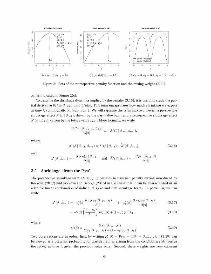
Figure 1 plots pen(β | βt−1) prospectively as a function of β, given the previous value βt−1. Itis also illuminating to plot pen(βt+1 | β) retrospectively as a function of β, given the future valueβt+1. Two such retrospective penalty plots are provided in Figure 2(a) and Figure 2(b). When thefuture value is relatively large (βt+1 = 1.5 in Figure 2(b)), the penalty pen(βt+1 | β) has a peaknear βt+1, signaling that the value βt must be large too. When the future value is small (βt+1 = 0

in Figure 2(a)), the penalty has a peak at zero signaling that the current value βt must have beensmall. Again, this balance is achieved with a relatively large stationary slab variance and a largeΘ.

The behavior of the prospective and retrospective penalties is ultimately tied to the mixingweight θt ≡ θ(β) in (2.11). It is desirable that θ(β) is increasing with |β|. However, Laplace tailswill begin to dominate for large enough |β|, where the probability θ(β) will begin to drop (for |β|greater than δ ≡ (λ0 +

√2C/A)A, where A = λ1/(1 − φ21) and C = log[(1 − Θ)/Θλ0/2

√2πA]).

However, we can make the turning point δ large enough with larger values Θ and smaller values

8

−2 −1 0 1 2 3

−2.

5−

2.0

−1.

5−

1.0

β

Ret

rosp

ectiv

e P

enal

tyRetrospective penalty

βt+1 = 0λ0 = 1φ1 = 0.9λ1 = 10(1 − φ1

2)Θ = 0.9

βt+1

(a) pen(β|βt+1 = 0)

−2 −1 0 1 2 3

−3.

5−

3.0

−2.

5−

2.0

−1.

5

β

Ret

rosp

ectiv

e P

enal

ty

Retrospective penalty

βt+1 = 1.5λ0 = 1φ1 = 0.9λ1 = 10(1 − φ1

2)Θ = 0.9

βt+1

(b) pen(β|βt+1 = 1.5)

−20 −10 0 10 20

0.0

0.2

0.4

0.6

0.8

1.0

β

θ(β)

Theta=0.1,lambda0=1Theta=0.9,lambda0=1Theta=0.9,lambda0=2

Transition weight (2.9)

(c) φ0 = 0, φ1 = 0.9, λ1 = 10(1− φ21)

Figure 2: Plots of the retrospective penalty function and the mixing weight (2.11)

λ0, as indicated in Figure 2(c).To describe the shrinkage dynamics implied by the penalty (3.15), it is useful to study the par-

tial derivative ∂Pen(β | βt−1, βt+1)/∂|β|. This term encapsulates how much shrinkage we expectat time t, conditionally on (βt−1, βt+1). We will separate the term into two pieces: a prospectiveshrinkage effect λ?(β | βt−1), driven by the past value βt−1, and a retrospective shrinkage effectλ?(β | βt+1), driven by the future value βt+1. More formally, we write

∂ Pen(β | βt−1, βt+1)

∂|β|≡ −Λ?(β | βt−1, βt+1),

whereΛ?(β | βt−1, βt+1) = λ?(β | βt−1) + λ?(β | βt+1), (3.16)

and

λ?(β | βt−1) = −∂ pen(β | βt−1)

∂|β|and λ?(β | βt+1) = −∂ pen(βt+1|β)

∂|β|.

3.1 Shrinkage “from the Past"

The prospective shrinkage term λ?(β | βt−1) pertains to Bayesian penalty mixing introduced byRockova (2017) and Rockova and George (2016) in the sense that it can be characterized as anadaptive linear combination of individual spike and slab shrinkage terms. In particular, we canwrite

λ?(β | βt−1) = −p?t (β)∂ logψ1(β | µt, λ1)

∂|β|− [1− p?t (β)]

∂ logψ0(β | λ0)

∂|β|, (3.17)

= p?t (β)

(β − µtλ1

)sign(β) + [1− p?t (β)]λ0 (3.18)

where

p?t (β) ≡ θtψ1(β | µt, λ1)

θtψ1(β | µt, λ1) + (1− θt)ψ0(β | λ0). (3.19)

Two observations are in order: first, by writing p?t (β) = P(γt = 1|βt = β, βt−1, θt), (3.19) canbe viewed as a posterior probability for classifying β as arising from the conditional slab (versusthe spike) at time t, given the previous value βt−1. Second, these weights are very different

9

from θt in (2.11), which are classifying β as arising from the marginal slab (versus the spike).From (3.19), we can see how p?t (β) hierarchically transmits information about the past value βt−1(via θt) to determine the right shrinkage for βt. This is achieved with a doubly-adaptive chainreaction. Namely, if the previous value βt−1 was large, θt will be close to one signaling that thenext coefficient βt is prone to be in the slab. Next, if βt is in fact large, p?t (βt) will be close toone, where the first summand in (3.17) becomes the leading term and shrinks βt towards µt. Ifβt is small, however, p?t (βt) will be small as well, where the second term in (3.17) takes over toshrink βt towards zero. This gravitational pull is accelerated when the previous value βt−1 wasnegligible (zero), in which case θt will be even smaller, making it even more difficult for the nextcoefficient βt to escape the spike. This mechanism explains how the prospective penalty adapts toboth (βt−1, βt), promoting smooth forward proliferation of spike/slab allocations and coefficients.

3.2 Shrinkage “from the Future"

While the prospective shrinkage term promotes smooth forward proliferation, the retrospectiveshrinkage term λ?(β | βt+1) operates backwards. We can write

λ?(β | βt+1) =− ∂θt+1

∂|β|

[p?t+1(βt+1)

θt+1−

1− p?t+1(βt+1)

1− θt+1

]− p?t+1(βt+1)φ1sign(β)

[βt+1 − µt+1

λ1

], (3.20)

where∂θt+1

∂|β|= θt+1(1− θt+1)

[λ0 − sign(β)

(β − φ0

λ1/(1− φ21)

)]. (3.21)

For simplicity, we will write p?t+1 = p?t+1(βt+1). Then we have

λ?(β | βt+1) =[λ0 − sign(β)

(β − φ0

λ1/(1− φ21)

)] [(1− p?t+1)θt+1 − p?t+1(1− θt+1)

](3.22)

− p?t+1φ1sign(β)

(βt+1 − µt+1

λ1

). (3.23)

The retrospective term synthesizes information from both (βt+1, βt) to contribute to shrinkage attime t. When (βt+1, βt) are both large, we obtain p?t (βt+1) and θt+1 that are both close to one. Theshrinkage is then driven by the second summand in (3.23), forcing βt to be shrunk towards thefuture value βt+1 (through µt+1 = φ0 + φ1(βt − φ0)). When either βt+1 or βt are small, shrinkageis targeted towards the stationary mean through the dominant term (3.22).

4 Characterization of the Joint Posterior Mode

Unlike previous developments (Nakajima and West 2013a; Kalli and Griffin 2014), this paperviews Bayesian dynamic shrinkage through the lens of optimization. Rather than distilling pos-terior samples to learn about B = [β1, . . . ,βT ], we focus on finding the MAP trajectory B =

arg maxπ(B |y). MAP sequence estimation problems (for non-linear non-Gaussian dynamic mod-els) were addressed previously with, e.g., Viterbi-style algorithms (Godsill et al. 2001). Our op-timization strategy is conceptually very different. The key to our approach will be drawing upon

10

the penalized likelihood perspective developed in Section 3. Namely, we develop a new dynamiccoordinate-wise strategy, building on existing developments for static high-dimensional variableselection.

4.1 The One-dimensional Case

To illustrate the functionality of the dynamic penalty from Section 3, we start by assuming p = 1

and xt = 1 in (1.1). This simple case corresponds to a sparse normal-means model, where themeans are dynamically intertwined. We begin by characterizing some basic properties of theposterior mode

β = arg maxβ

π(β|y),

where y = (y1, . . . , yT )′ arises from (1.1) and β = (β1, . . . , βT )′ is assigned the DSS prior.One of the attractive features of the Laplace spike in (2.5) is that β has a thresholding property.

This property is revealed from necessary characterizations for each βt (for t = 1, . . . , T ), once wecondition on the rest of the directions through (βt−1, βt+1). The conditional thresholding rule canbe characterized using standard arguments, as with similar existing regularizers (Zhang 2010; Fanand Li 2001; Antoniadis and Fan 2001; Zhang and Zhang 2012; Rockova and George 2016). Whilethe typical sparsity-inducing penalty functions are symmetric, the penalty (3.15) is not, due to itsdependence on the previous and future values (βt−1, βt+1). Thereby, instead of a single selectionthreshold, we have two:

∆−(x, βt−1, βt+1) = supβ<0

{βx2

2+Pen(β | βt−1, βt+1)

β

}(4.24)

∆+(x, βt−1, βt+1) = infβ>0

{βx2

2+Pen(β | βt−1, βt+1)

β

}. (4.25)

The following necessary characterization links the behavior of β to the shrinkage terms char-acterized in Section 3.1 and Section 3.2.

Lemma 1. Denote by β = (β1, . . . , βT )′ the global mode of π(β|y) and by ∆−t and ∆−t the selectionthresholds (4.24) and (4.25) with x = 1, βt−1 = βt−1 and βt+1 = βt+1. Then, conditionally on(βt−1, βt+1), we have for 1 < t < T

βt =

0 if ∆−t < yt < ∆+t

[|yt| − Λ?(βt | βt−1, βt+1)]+ sign(yt) otherwise,(4.26)

where Λ?(βt | βt−1, βt+1) was defined in (3.16).

Proof. We begin by noting that βt is a maximizer in tth direction while keeping (βt−1, βt+1) fixed,i.e.

βt = arg maxβ

{−1

2(yt − β)2 + Pen(β | βt−1, βt+1)

}. (4.27)

It turns out that βt = 0 iff β(β2 + Pen(β | βt−1,βt+1)

β − yt)< 0, ∀β ∈ R\{0} (Zhang and Zhang

2012). The rest of the proof follows from the definition of ∆+t and ∆−t in (4.24) and (4.25).

Conditionally on (βt−1, βt+1), the global mode βt, once nonzero, has to satisfy (4.26) from thefirst-order necessary condition.

11

Lemma 1 formally certifies that the mode exhibits both (a) sparsity and (b) smoothness (throughthe prospective/retrospective shrinkage terms).

Remark 3. While Lemma 1 assumes 1 < t < T , the characterization applies also for t = 1, oncewe specify the initial condition βt=0. The value βt=0 is not assumed known and will be estimatedtogether with all the remaining parameters (Section 5). For t = T , an analogous characterizationexists, where the shrinkage term and the selection threshold only contain the prospective portion ofthe penalty.

4.2 General Regression

When p > 1, there is a delicate interplay between the multiple series, where overfitting in onedirection may impair recovery in other directions. As will be seen in Section 6, anchoring onsparsity is a viable remedy to these issues. We obtain analogous characterizations of the globalmode. We will denote with ∆−tj and ∆−tj the selection thresholds (4.24) and (4.25) with x =

xtj , βt−1 = βt−1j , and βt+1 = βt+1j .

Lemma 2. Denote by B = {βtj}T,pt,j=1 the global mode of π(B|Y ), by B tj all but the (t, j)th entryin B and by ztj = yt −

∑i 6=j xtiβti. Let Ztj = xtjztj . Then βtj satisfies the following necessary

condition

βtj =

1x2tj

[Ztj − Λ?(βtj | βt−1j , βt−1j)]+ sign(Ztj) if ∆−tj < Ztj < ∆+tj

0 otherwise.

Proof. Follows from Lemma 1, noting that βtj is a maximizer in (t, j)th direction while keepingB tj fixed, i.e.

βtj = arg maxβ

{−1

2(ztj − xtjβ)2 + Pen(β | βt−1j , βt+1j)

}. (4.28)

Lemma 2 evokes coordinate-wise optimization for obtaining the posterior mode. However, thecomputation of selection thresholds (∆−tj ,∆

+tj) (as well as the one-site maximizers (4.27)) requires

numerical optimization. The lack of availability of closed-form thresholding hampers practicalitywhen T and p are even moderately large. In the next section, we propose an alternative strategywhich capitalizes on closed-form thresholding rules.

5 One-step-late EM Algorithm

A (local) posterior mode B can be obtained either directly, by cycling over one-site updates (4.28),or indirectly through an EM algorithm, a strategy pursued here. The direct algorithm consists ofintegrating out G = [γ1, . . . ,γT ]′ and solving a sequence of non-standard optimization problems(4.28), which necessitate numerical optimization. The EM algorithm, on the other hand, treatsG as missing data, obviating the need for numerical optimization by offering closed form one-siteupdates. We now describe this dynamic EM approach for MAP estimation under DSS priors.

The initial vector βt=0 = (β01, . . . , β0p)′ at time t = 0 will be estimated together with all the

remaining coefficients B. We assume that β0 comes from the stationary distribution described in

12

Theorem 1

π(β0|γ0) =

p∏j=1

[γ0jψ

ST1 (β0j | λ1, φ0, φ1) + (1− γ0j)ψ0(β0j | λ0)

], (5.29)

where γ0 = (γ01, . . . , γ0p)′ are independent binary indicators with P[γ0j = 1 |Θ] = Θ for 1 ≤ j ≤ p.

Knowing the stationary distribution, thus, has advantages for specifying the initial conditions. Thegoal is obtaining the joint mode [B, β0] of the functional π(B,β0|Y ). To this end, we proceediteratively by augmenting this objective function with the missing data [G,γ0], as prescribed byRockova and George (2014), and then maximizing w.r.t. [B,β0]. An important observation, thatfacilitates the derivation of the algorithm, is that the prior distribution π(β0,B,γ0,G) can befactorized into the following products

π(β0,B,γ0,G) = π(β0|γ0)

p∏j=1

T∏t=1

π(βtj |γtj , βt−1j)π(γtj |βt−1j),

where π(βtj |γtj , βt−1j) and π(γtj |βt−1j) are defined in (2.5) and (2.7), respectively. For simplicity(and without loss of generality), we will assume φ0 = 0 and thereby µtj = φ1βt−1j . Then, we canwrite

log π(β0,B,γ0,G|Y ) = C +

T∑t=1

p∑j=1

[γtj log θtj + (1− γtj) log(1− θtj)] (5.30)

−T∑t=1

(yt − x′tβt)2

2+

p∑j=1

[γtj

(βtj − φ1βt−1j)2

2λ1+ (1− γtj)λ0|βtj |

]−

p∑j=1

[γ0j

β20j(1− φ21)

2λ1+ (1− γ0j)λ0|β0j | − γ0j log Θ− (1− γ0j) log(1−Θ)

].

We will endow the parameters [β0,B] with a superscript m to designate their most recent valuesat the mth iteration. In the E-step, we compute the expectation E γ0,G|·

log π(β0,B,γ0,G|Y )

with respect to the conditional distribution of [G,γ0], given [B(m),β(m)0 ] and Y . All we have to

really do is obtain p?tj = P(γtj = 1|β(m)tj , β

(m)t−1j , θtj) from (3.19), when t > 0, and p?0j ≡ θ1j ≡

θ(β0j) from (2.11), and replace all the γtj ’s in (5.30) with p?tj ’s. In the M-step, we set out tomaximize E γ0,G|·

log π(β0,B,γ0,G|Y ) w.r.t. [β0,B]. We proceed coordinate-wise, iterating overthe following single-site updates while keeping all the remaining parameters fixed. For 1 < t < T ,we have

β(m+1)tj = arg max

βQtj(β),

where

Qtj(β) =− 1

2(ztj − xtjβ)2 −

p?tj2λ1

(β − φ1β(m)t−1j)

2 −p?t+1j

2λ1(β

(m)t+1j − φ1β)2

− (1− p?tj)λ0|β|+ p?t+1j log θt+1j + (1− p?t+1j) log(1− θt+1j), (5.31)

and where ztj = yt −∑i 6=j xtiβ

(m)ti . From the first-order condition, the solution β

(m+1)tj , if

nonzero, needs to satisfy ∂Qtj(β)/∂β∣∣β=β

(m+1)tj

= 0. To write the derivative slightly more con-

cisely, we introduce the following notation: Ztj = xtjztj +p?tjφ1

λ1β(m+1)t−1j +

p?t+1jφ1

λ1β(m+1)t+1j and

13

Wtj =(x2tj +

p?tjλ1

+p?t+1jφ

21

λ1

). Then we can write for β 6= 0

∂Qtj(β)

∂β=Ztj −Wtjβ − (1− p?tj)λ0 sign(β) +

∂θt+1j

∂β

[p?t+1j

θt+1j−

1− p?t+1j

1− θt+1j

], (5.32)

where∂θt+1j

∂β= θt+1j(1− θt+1j)

[λ0 sign(β)− β(1− φ21)

λ1

]is obtained from (3.21). Recall that θt+1j , defined in (2.11), depends on βtj (denoted by β above).This complicates the tractability of the M-step. If θt+1j was fixed, we could obtain a simple closed-form solution β

(m+1)tj through an elastic-net-like update (Zou and Hastie 2005). We can take

advantage of this fact with a one-step-late (OSL) adaptation of the EM algorithm (Green 1990).The OSL EM algorithm bypasses intricate M-steps by evaluating the intractable portions of thepenalty derivative at the most recent value, rather than the new value. We apply this trick to thelast summand in (5.32). Instead of treating θt+1j as a function of β in (5.32), we fix it at the mostrecent value β(m)

tj . The solution for β, implied by (5.32), is then

β(m+1)tj =

1

Wtj + (1− φ21)/λ1Mtj[Ztj − Λtj ]+ sign(Ztj), for 1 < t < T, (5.33)

where Mtj = p?t+1j(1 − θt+1j) − θt+1j(1 − p?t+1j) and Λtj = λ0[(1 − p?tj) − Mtj ]. The update

(5.33) is a thresholding rule, with a shrinkage term that reflects the size of (β(m)t−1j , β

(m)tj , β

(m)t+1j).

The exact thresholding property is obtained from sub-differential calculus, because Qtj(·) is notdifferentiable at zero (due to the Laplace spike). A very similar update is obtained also for t = T ,where all the terms involving p?t+1j and θt+1j in Λtj ,Wtj and Ztj disappear. For t = 0, we have

β(m+1)0j =

1

p?1jφ21 + p?0j(1− φ21)

[p?0jβ1jφ1 − (1− p?0j)λ0λ1

]+

sign(β1j). (5.34)

The updates (5.33) and (5.34) can be either cycled-over at each M-step, or performed just oncefor each M-step.

Remark 4. For autoregression with a higher order h > 1, the retrospective penalty would be similarwhere µt would depend on h lagged values. The prospective penalty would consist of not just one, buth terms. For the EM implementation, one would proceed analogously by evaluating the derivatives ofθt+1, . . . , θt+h w.r.t. β at the most recent update of the process from the previous iteration and keepthem fixed for each one-site update.

To illustrate the ability of theDSS priors to suppress noise and recover true signal, we considera high-dimensional synthetic dataset and a topical macroeconomic dataset.

6 Synthetic High-Dimensional Data

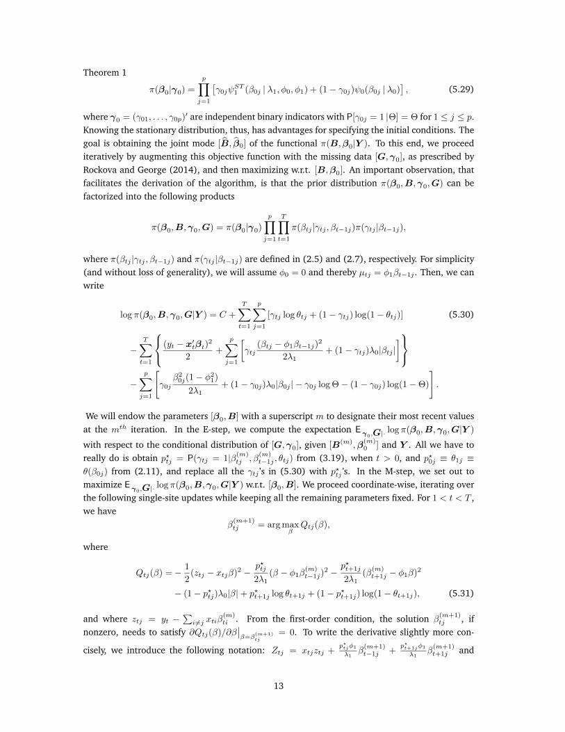
We first illustrate our dynamic variable selection procedure on a simulated example with T = 100

observations generated from the model (1.1) with p = 50 predictors. The predictor values xtjare obtained independently from a standard normal distribution. Out of the 50 predictors, 46

never contribute to the model (predictors xt5 through xt50), where β0t5 = β0

t6 = ... = β0t50 = 0

at all times. The predictor xt1 is a persisting predictor, where {βt1}Tt=1 is generated according

14

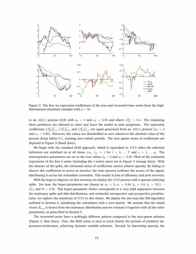
Figure 3: The first six regression coefficients of the true and recovered time series from the high-dimensional simulated example with p = 50.

to an AR(1) process (2.8) with φ0 = 0 and φ1 = 0.98 and where |β0t1| > 0.5. The remaining

three predictors are allowed to enter and leave the model as time progresses. The regressioncoefficients {β0

t2}Tt=1, {β0t3}Tt=1 and {β0

t4}Tt=1 are again generated from an AR(1) process (φ0 = 0

and φ1 = 0.98). However, the values are thresholded to zero whenever the absolute value of theprocess drops below 0.5, creating zero-valued periods. The true sparse series of coefficients aredepicted in Figure 3 (black lines).

We begin with the standard DLM approach, which is equivalent to DSS when the selectionindicators are switched on at all times, i.e., γtj = 1 for t = 0, . . . , T and j = 1, . . . , p. Theautoregressive parameters are set to the true values φ0 = 0 and φ1 = 0.98. Plots of the estimatedtrajectories of the first 6 series (including the 4 active ones) are in Figure 3 (orange lines). Withthe absence of the spike, the estimated series of coefficients cannot achieve sparsity. By failing todiscern the coefficients as active or inactive, the state process confuses the source of the signal,distributing it across the redundant covariates. This results in loss of efficiency and poor recovery.

With the hope to improve on this recovery, we deploy the DSS process with a sparsity inducingspike. For now, the hyper-parameters are chosen as φ0 = 0, φ1 = 0.98, λ0 = 0.9, λ1 = 25(1 −φ21), and Θ = 0.98. This hyper-parameter choice corresponds to a very mild separation betweenthe stationary spike and slab distributions, and unimodal retrospective and prospective penalties.Later, we explore the sensitivity of DSS to this choice. We deploy the one-step-late EM algorithmoutlined in Section 5, initializing the calculation with a zero matrix. We assume that the initialvector βt=0 is drawn from the stationary distribution and we estimate it together with all the otherparameters, as prescribed in Section 5.

The recovered series have a strikingly different pattern compared to the non-sparse solution(Figure 3, blue lines). First, the MAP series is seen to track closely the periods of predictor im-portance/irrelevance, achieving dynamic variable selection. Second, by harvesting sparsity, the

15

Figure 4: Mixing weights θtj , defined in (2.11), for the simulated examples in Section 6 for thefirst six series.

DSS priors alleviate bias in the nonzero directions, outputting a cleaner representation of thetrue underlying signal.

We also compare the performance to the NGAR process of Kalli and Griffin (2014) and theLASSO method. The latter does not take into account the temporal nature of the problem. ForNGAR, we use the default settings, b∗ = s∗ = 0.1, with 1,000 burn-in and 1,000 MCMC iterations.For LASSO, we sequentially run a static regression in an extending window fashion, where theLASSO regression is refit using 1 : t for each t = 1 : T to produce a series of quasi-dynamiccoefficients; a common practice for using static shrinkage methods for time series data (Bai andNg 2008; De Mol et al. 2008; Stock and Watson 2012; Li and Chen 2014), choosing λ via 10-foldcross-validation.

For the first series, the only persistent series, we see that both NGAR and DSS succeed wellin tracing the true signal. This is especially true in contrast to DLM and LASSO, which bothsignificantly under-valuate the signal. The estimated coefficient evolutions for DLM and LASSObecome inconclusive for assessing variable importance, where the coefficient estimates for therelevant variables have been reduced by the increased estimates for the irrelevant variables. Forthe second to fourth series with intermittent zeros, we see that DSS is the only method ableto separate the true zero/nonzero signal (noted by the flat coefficient estimates during inactiveperiods). On the other hand, NGAR seems to be not shrinking enough, instead smoothing theseries as if curve-fitting. The LASSO method produces sparse estimates, however the variableselection is not linked over time and thereby erratic. For the two zero series (series five andsix), it is clear that DSS is the only method that truly shrinks noise to zero. The DSS priorsmitigate overfitting by eliminating noisy coefficients and thereby leaving enough room for thetrue predictors to capture the trend. As a revealing byproduct, we also obtain the evolving mixingweights determining the relevance of each coefficient at each time. The evolutions of rescaled

16

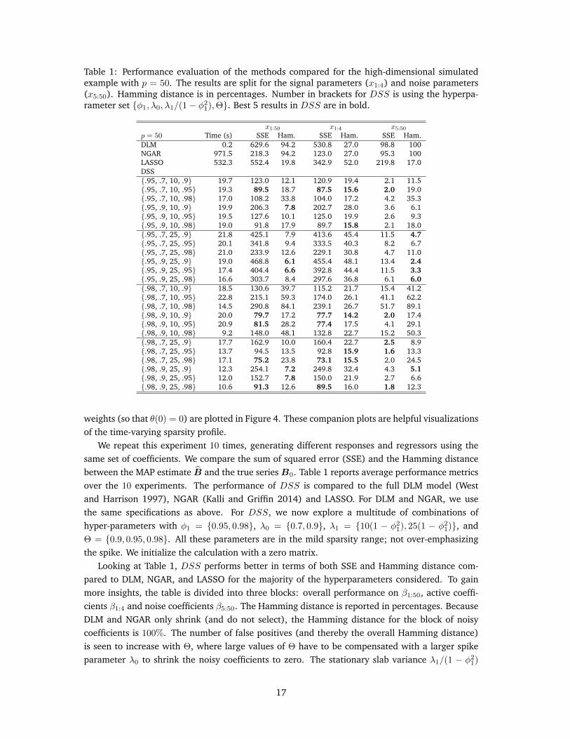
Table 1: Performance evaluation of the methods compared for the high-dimensional simulatedexample with p = 50. The results are split for the signal parameters (x1:4) and noise parameters(x5:50). Hamming distance is in percentages. Number in brackets for DSS is using the hyperpa-rameter set {φ1, λ0, λ1/(1− φ21),Θ}. Best 5 results in DSS are in bold.

x1:50 x1:4 x5:50p = 50 Time (s) SSE Ham. SSE Ham. SSE Ham.DLM 0.2 629.6 94.2 530.8 27.0 98.8 100NGAR 971.5 218.3 94.2 123.0 27.0 95.3 100LASSO 532.3 552.4 19.8 342.9 52.0 219.8 17.0DSS{.95, .7, 10, .9} 19.7 123.0 12.1 120.9 19.4 2.1 11.5{.95, .7, 10, .95} 19.3 89.5 18.7 87.5 15.6 2.0 19.0{.95, .7, 10, .98} 17.0 108.2 33.8 104.0 17.2 4.2 35.3{.95, .9, 10, .9} 19.9 206.3 7.8 202.7 28.0 3.6 6.1{.95, .9, 10, .95} 19.5 127.6 10.1 125.0 19.9 2.6 9.3{.95, .9, 10, .98} 19.0 91.8 17.9 89.7 15.8 2.1 18.0{.95, .7, 25, .9} 21.8 425.1 7.9 413.6 45.4 11.5 4.7{.95, .7, 25, .95} 20.1 341.8 9.4 333.5 40.3 8.2 6.7{.95, .7, 25, .98} 21.0 233.9 12.6 229.1 30.8 4.7 11.0{.95, .9, 25, .9} 19.0 468.8 6.1 455.4 48.1 13.4 2.4{.95, .9, 25, .95} 17.4 404.4 6.6 392.8 44.4 11.5 3.3{.95, .9, 25, .98} 16.6 303.7 8.4 297.6 36.8 6.1 6.0{.98, .7, 10, .9} 18.5 130.6 39.7 115.2 21.7 15.4 41.2{.98, .7, 10, .95} 22.8 215.1 59.3 174.0 26.1 41.1 62.2{.98, .7, 10, .98} 14.5 290.8 84.1 239.1 26.7 51.7 89.1{.98, .9, 10, .9} 20.0 79.7 17.2 77.7 14.2 2.0 17.4{.98, .9, 10, .95} 20.9 81.5 28.2 77.4 17.5 4.1 29.1{.98, .9, 10, .98} 9.2 148.0 48.1 132.8 22.7 15.2 50.3{.98, .7, 25, .9} 17.7 162.9 10.0 160.4 22.7 2.5 8.9{.98, .7, 25, .95} 13.7 94.5 13.5 92.8 15.9 1.6 13.3{.98, .7, 25, .98} 17.1 75.2 23.8 73.1 15.5 2.0 24.5{.98, .9, 25, .9} 12.3 254.1 7.2 249.8 32.4 4.3 5.1{.98, .9, 25, .95} 12.0 152.7 7.8 150.0 21.9 2.7 6.6{.98, .9, 25, .98} 10.6 91.3 12.6 89.5 16.0 1.8 12.3

weights (so that θ(0) = 0) are plotted in Figure 4. These companion plots are helpful visualizationsof the time-varying sparsity profile.

We repeat this experiment 10 times, generating different responses and regressors using thesame set of coefficients. We compare the sum of squared error (SSE) and the Hamming distancebetween the MAP estimate B and the true seriesB0. Table 1 reports average performance metricsover the 10 experiments. The performance of DSS is compared to the full DLM model (Westand Harrison 1997), NGAR (Kalli and Griffin 2014) and LASSO. For DLM and NGAR, we usethe same specifications as above. For DSS, we now explore a multitude of combinations ofhyper-parameters with φ1 = {0.95, 0.98}, λ0 = {0.7, 0.9}, λ1 = {10(1 − φ21), 25(1 − φ21)}, andΘ = {0.9, 0.95, 0.98}. All these parameters are in the mild sparsity range; not over-emphasizingthe spike. We initialize the calculation with a zero matrix.

Looking at Table 1, DSS performs better in terms of both SSE and Hamming distance com-pared to DLM, NGAR, and LASSO for the majority of the hyperparameters considered. To gainmore insights, the table is divided into three blocks: overall performance on β1:50, active coeffi-cients β1:4 and noise coefficients β5:50. The Hamming distance is reported in percentages. BecauseDLM and NGAR only shrink (and do not select), the Hamming distance for the block of noisycoefficients is 100%. The number of false positives (and thereby the overall Hamming distance)is seen to increase with Θ, where large values of Θ have to be compensated with a larger spikeparameter λ0 to shrink the noisy coefficients to zero. The stationary slab variance λ1/(1 − φ21)

17

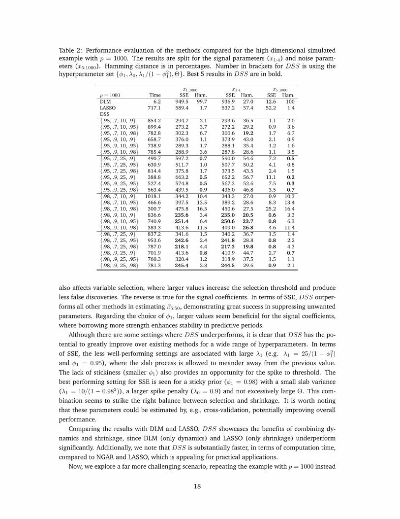
Table 2: Performance evaluation of the methods compared for the high-dimensional simulatedexample with p = 1000. The results are split for the signal parameters (x1:4) and noise param-eters (x5:1000). Hamming distance is in percentages. Number in brackets for DSS is using thehyperparameter set {φ1, λ0, λ1/(1− φ21),Θ}. Best 5 results in DSS are in bold.

x1:1000 x1:4 x5:1000p = 1000 Time SSE Ham. SSE Ham. SSE Ham.DLM 6.2 949.5 99.7 936.9 27.0 12.6 100LASSO 717.1 589.4 1.7 537.2 57.4 52.2 1.4DSS{.95, .7, 10, .9} 854.2 294.7 2.1 293.6 36.5 1.1 2.0{.95, .7, 10, .95} 899.4 273.2 3.7 272.2 29.2 0.9 3.6{.95, .7, 10, .98} 782.8 302.3 6.7 300.6 19.2 1.7 6.7{.95, .9, 10, .9} 658.7 376.0 1.1 373.9 43.0 2.1 0.9{.95, .9, 10, .95} 738.9 289.3 1.7 288.1 35.4 1.2 1.6{.95, .9, 10, .98} 785.4 288.9 3.6 287.8 28.6 1.1 3.5{.95, .7, 25, .9} 490.7 597.2 0.7 590.0 54.6 7.2 0.5{.95, .7, 25, .95} 630.9 511.7 1.0 507.7 50.2 4.1 0.8{.95, .7, 25, .98} 814.4 375.8 1.7 373.5 43.5 2.4 1.5{.95, .9, 25, .9} 388.8 663.2 0.5 652.2 56.7 11.1 0.2{.95, .9, 25, .95} 527.4 574.8 0.5 567.3 52.6 7.5 0.3{.95, .9, 25, .98} 563.4 439.5 0.9 436.0 46.8 3.5 0.7{.98, .7, 10, .9} 1018.1 344.2 10.4 343.3 27.0 0.9 10.3{.98, .7, 10, .95} 466.6 397.5 13.5 389.2 28.6 8.3 13.4{.98, .7, 10, .98} 300.7 475.8 16.5 450.6 27.5 25.2 16.4{.98, .9, 10, .9} 836.6 235.6 3.4 235.0 20.5 0.6 3.3{.98, .9, 10, .95} 740.9 251.4 6.4 250.6 23.7 0.8 6.3{.98, .9, 10, .98} 383.3 413.6 11.5 409.0 26.8 4.6 11.4{.98, .7, 25, .9} 837.2 341.6 1.5 340.2 36.7 1.5 1.4{.98, .7, 25, .95} 953.6 242.6 2.4 241.8 28.8 0.8 2.2{.98, .7, 25, .98} 787.0 218.1 4.4 217.3 19.8 0.8 4.3{.98, .9, 25, .9} 701.9 413.6 0.8 410.9 44.7 2.7 0.7{.98, .9, 25, .95} 760.3 320.4 1.2 318.9 37.5 1.5 1.1{.98, .9, 25, .98} 781.3 245.4 2.3 244.5 29.6 0.9 2.1

also affects variable selection, where larger values increase the selection threshold and produceless false discoveries. The reverse is true for the signal coefficients. In terms of SSE, DSS outper-forms all other methods in estimating β5:50, demonstrating great success in suppressing unwantedparameters. Regarding the choice of φ1, larger values seem beneficial for the signal coefficients,where borrowing more strength enhances stability in predictive periods.

Although there are some settings where DSS underperforms, it is clear that DSS has the po-tential to greatly improve over existing methods for a wide range of hyperparameters. In termsof SSE, the less well-performing settings are associated with large λ1 (e.g. λ1 = 25/(1 − φ21)

and φ1 = 0.95), where the slab process is allowed to meander away from the previous value.The lack of stickiness (smaller φ1) also provides an opportunity for the spike to threshold. Thebest performing setting for SSE is seen for a sticky prior (φ1 = 0.98) with a small slab variance(λ1 = 10/(1 − 0.982)), a larger spike penalty (λ0 = 0.9) and not excessively large Θ. This com-bination seems to strike the right balance between selection and shrinkage. It is worth notingthat these parameters could be estimated by, e.g., cross-validation, potentially improving overallperformance.

Comparing the results with DLM and LASSO, DSS showcases the benefits of combining dy-namics and shrinkage, since DLM (only dynamics) and LASSO (only shrinkage) underperformsignificantly. Additionally, we note that DSS is substantially faster, in terms of computation time,compared to NGAR and LASSO, which is appealing for practical applications.

Now, we explore a far more challenging scenario, repeating the example with p = 1000 instead

18

of 50. The coefficients and data generating process are the same with p = 50, but now insteadof 46 noise regressors, we have 996. This high regressor redundancy rate is representative of the“p >> n" paradigm (“p >> T " for time series data) and can test the limits of any sparsity inducingprocedure. Under this setting, we will be able to truly evaluate the efficacy of DSS and compareit to other methods when there is a large number of predictors with sparse signals.

The results are collated in Table 2. The same set of hyperparameters that performed best forp = 50 also does extremely well for p = 1000, dramatically reducing SSE over DLM and LASSO.We have not reported comparisons to NGAR, because it did not seem to produce reliable/sensibleresults in this high-dimensional scenario. Due to a long running time, we had to consider onlyshort MCMC chains which produced unstable and un-reportable results. In addition, we did notattempt to tune the hyper-parameters and used the default options in the matlab program providedby the authors. On the other hand, DSS produces reasonable estimates, improving upon DLM andLASSO (for the majority of settings). We also note that, while LASSO does perform well in termsof the Hamming distance, it does not do so well in terms of SSE. Because LASSO lacks dynamics,the pattern of sparsity is not smooth over time, leading to erratic coefficient evolutions. Becauseof the smooth nature of its sparsity, DSS harnesses the dynamics to discern signal from noise,improving in both SSE and Hamming distance.

7 High-Dimensional Macroeconomic Data

We further illustrate the effectiveness of DSS through a topical macroeconomic dataset from Mc-Cracken and Ng (2016), which consists of 119 monthly macroeconomic variables over the spanof 1986/1 to 2015/12. There are eight primary groups that comprise this dataset: Output and In-come, Labor Market, Consumption and Orders, Orders and Inventories, Money and Credit, InterestRate and Exchange Rates, Prices, and Stock Market. Details of the descriptions and transforma-tions of the predictors can be found in the Appendix of McCracken and Ng (2016).

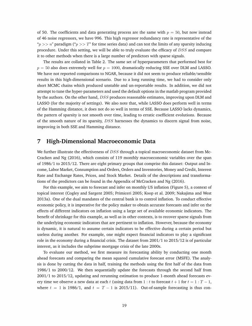
For this example, we aim to forecast and infer on monthly US inflation (Figure 5), a context oftopical interest (Cogley and Sargent 2005; Primiceri 2005; Koop et al. 2009; Nakajima and West2013a). One of the dual mandates of the central bank is to control inflation. To conduct effectiveeconomic policy, it is imperative for the policy maker to obtain accurate forecasts and infer on theeffects of different indicators on inflation using a large set of available economic indicators. Thebenefit of shrinkage for this example, as well as in other contexts, is to recover sparse signals fromthe underlying economic indicators that are pertinent to inflation. However, because the economyis dynamic, it is natural to assume certain indicators to be effective during a certain period butuseless during another. For example, one might expect financial indicators to play a significantrole in the economy during a financial crisis. The dataset from 2001/1 to 2015/12 is of particularinterest, as it includes the subprime mortgage crisis of the late 2000s.

To evaluate our method, we first measure its forecasting ability by conducting one monthahead forecasts and comparing the mean squared cumulative forecast error (MSFE). The analy-sis is done by cutting the data in half, training the methods using the first half of the data from1986/1 to 2000/12. We then sequentially update the forecasts through the second half from2001/1 to 2015/12, updating and rerunning estimation to produce 1-month ahead forecasts ev-ery time we observe a new data at each t (using data from 1 : t to forecast t+ 1 for t = 1 : T − 1,where t = 1 is 1986/1, and t = T − 1 is 2015/11). Out-of-sample forecasting is thus con-

19

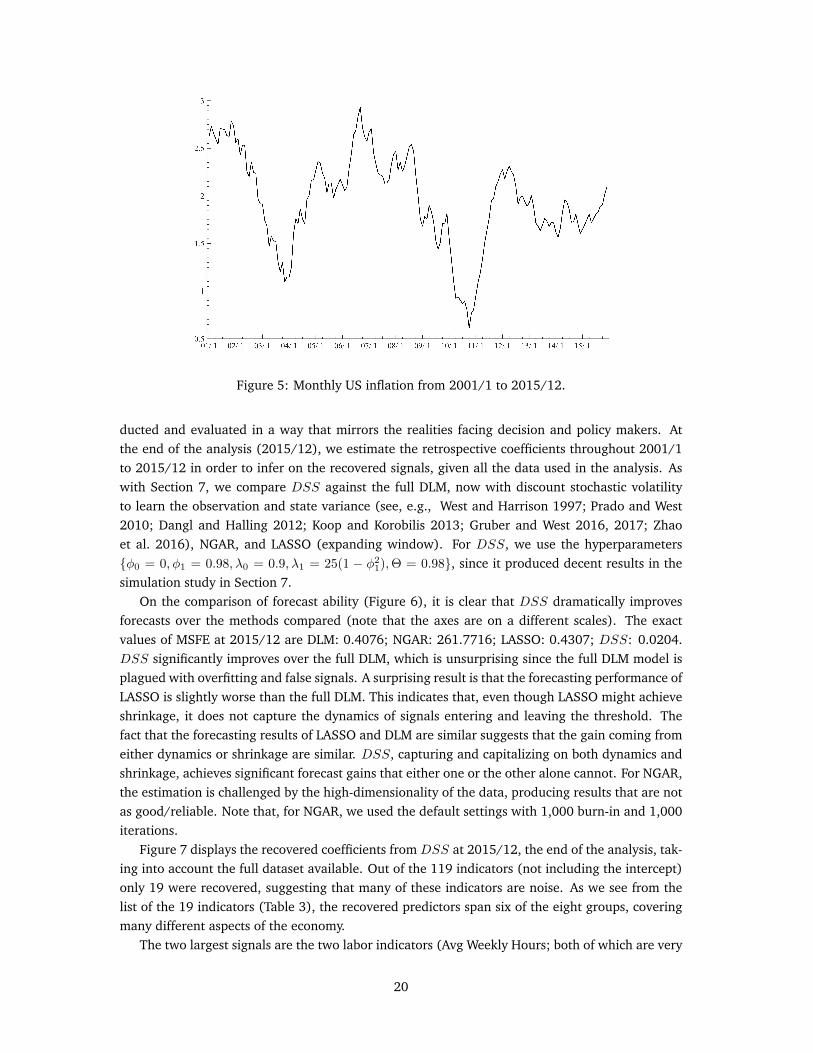
Figure 5: Monthly US inflation from 2001/1 to 2015/12.

ducted and evaluated in a way that mirrors the realities facing decision and policy makers. Atthe end of the analysis (2015/12), we estimate the retrospective coefficients throughout 2001/1to 2015/12 in order to infer on the recovered signals, given all the data used in the analysis. Aswith Section 7, we compare DSS against the full DLM, now with discount stochastic volatilityto learn the observation and state variance (see, e.g., West and Harrison 1997; Prado and West2010; Dangl and Halling 2012; Koop and Korobilis 2013; Gruber and West 2016, 2017; Zhaoet al. 2016), NGAR, and LASSO (expanding window). For DSS, we use the hyperparameters{φ0 = 0, φ1 = 0.98, λ0 = 0.9, λ1 = 25(1 − φ21),Θ = 0.98}, since it produced decent results in thesimulation study in Section 7.

On the comparison of forecast ability (Figure 6), it is clear that DSS dramatically improvesforecasts over the methods compared (note that the axes are on a different scales). The exactvalues of MSFE at 2015/12 are DLM: 0.4076; NGAR: 261.7716; LASSO: 0.4307; DSS: 0.0204.DSS significantly improves over the full DLM, which is unsurprising since the full DLM model isplagued with overfitting and false signals. A surprising result is that the forecasting performance ofLASSO is slightly worse than the full DLM. This indicates that, even though LASSO might achieveshrinkage, it does not capture the dynamics of signals entering and leaving the threshold. Thefact that the forecasting results of LASSO and DLM are similar suggests that the gain coming fromeither dynamics or shrinkage are similar. DSS, capturing and capitalizing on both dynamics andshrinkage, achieves significant forecast gains that either one or the other alone cannot. For NGAR,the estimation is challenged by the high-dimensionality of the data, producing results that are notas good/reliable. Note that, for NGAR, we used the default settings with 1,000 burn-in and 1,000iterations.

Figure 7 displays the recovered coefficients from DSS at 2015/12, the end of the analysis, tak-ing into account the full dataset available. Out of the 119 indicators (not including the intercept)only 19 were recovered, suggesting that many of these indicators are noise. As we see from thelist of the 19 indicators (Table 3), the recovered predictors span six of the eight groups, coveringmany different aspects of the economy.

The two largest signals are the two labor indicators (Avg Weekly Hours; both of which are very

20

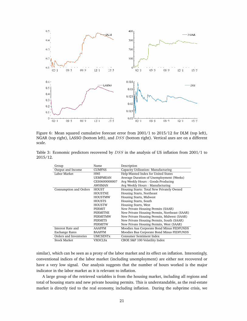
Figure 6: Mean squared cumulative forecast error from 2001/1 to 2015/12 for DLM (top left),NGAR (top right), LASSO (bottom left), and DSS (bottom right). Vertical axes are on a differentscale.

Table 3: Economic predictors recovered by DSS in the analysis of US inflation from 2001/1 to2015/12.

Group Name DescriptionOutput and Income CUMFNS Capacity Utilization: ManufacturingLabor Market HWI Help-Wanted Index for United States

UEMPMEAN Average Duration of Unemployment (Weeks)CES0600000007 Avg Weekly Hours : Goods-ProducingAWHMAN Avg Weekly Hours : Manufacturing

Consumption and Orders HOUST Housing Starts: Total New Privately OwnedHOUSTNE Housing Starts, NortheastHOUSTMW Housing Starts, MidwestHOUSTS Housing Starts, SouthHOUSTW Housing Starts, WestPERMIT New Private Housing Permits (SAAR)PERMITNE New Private Housing Permits, Northeast (SAAR)PERMITMW New Private Housing Permits, Midwest (SAAR)PERMITS New Private Housing Permits, South (SAAR)PERMITW New Private Housing Permits, West (SAAR)

Interest Rate and AAAFFM Moodies Aaa Corporate Bond Minus FEDFUNDSExchange Rates BAAFFM Moodies Baa Corporate Bond Minus FEDFUNDSOrders and Inventories UMCSENTx Consumer Sentiment IndexStock Market VXOCLSx CBOE S&P 100 Volatility Index

similar), which can be seen as a proxy of the labor market and its effect on inflation. Interestingly,conventional indices of the labor market (including unemployment) are either not recovered orhave a very low signal. Our analysis suggests that the number of hours worked is the majorindicator in the labor market as it is relevant to inflation.

A large group of the retrieved variables is from the housing market, including all regions andtotal of housing starts and new private housing permits. This is understandable, as the real-estatemarket is directly tied to the real economy, including inflation. During the subprime crisis, we

21

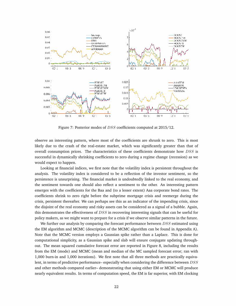
Figure 7: Posterior modes of DSS coefficients computed at 2015/12.

observe an interesting pattern, where most of the coefficients are shrunk to zero. This is mostlikely due to the crash of the real-estate market, which was significantly greater than that ofoverall consumption prices. The characteristics of these coefficients demonstrate how DSS issuccessful in dynamically shrinking coefficients to zero during a regime change (recession) as wewould expect to happen.

Looking at financial indices, we first note that the volatility index is persistent throughout theanalysis. The volatility index is considered to be a reflection of the investor sentiment, so thepersistence is unsurprising. The financial market is undoubtedly linked to the real economy, andthe sentiment towards one should also reflect a sentiment to the other. An interesting patternemerges with the coefficients for the Baa and (to a lesser extent) Aaa corporate bond rates. Thecoefficients shrink to zero right before the subprime mortgage crisis and reemerge during thecrisis, persistent thereafter. We can perhaps see this as an indicator of the impending crisis, sincethe disjoint of the real economy and risky assets can be considered as a signal of a bubble. Again,this demonstrates the effectiveness of DSS in recovering interesting signals that can be useful forpolicy makers, as we might want to prepare for a crisis if we observe similar patterns in the future.

We further our analysis by comparing the forecast performance between DSS estimated usingthe EM algorithm and MCMC (description of the MCMC algorithm can be found in Appendix A).Note that the MCMC version employs a Gaussian spike rather than a Laplace. This is done forcomputational simplicity, as a Gaussian spike and slab will ensure conjugate updating through-out. The mean squared cumulative forecast error are reported in Figure 8, including the resultsfrom the EM (mode) and MCMC (mean and median of the MC sampled forecast error; ran with1,000 burn-in and 1,000 iterations). We first note that all three methods are practically equiva-lent, in terms of predictive performance– especially when considering the difference betweenDSSand other methods compared earlier– demonstrating that using either EM or MCMC will producenearly equivalent results. In terms of computation speed, the EM is far superior, with EM clocking

22

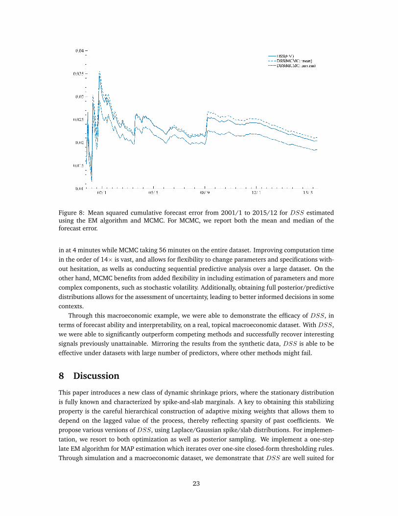
Figure 8: Mean squared cumulative forecast error from 2001/1 to 2015/12 for DSS estimatedusing the EM algorithm and MCMC. For MCMC, we report both the mean and median of theforecast error.

in at 4 minutes while MCMC taking 56 minutes on the entire dataset. Improving computation timein the order of 14× is vast, and allows for flexibility to change parameters and specifications with-out hesitation, as wells as conducting sequential predictive analysis over a large dataset. On theother hand, MCMC benefits from added flexibility in including estimation of parameters and morecomplex components, such as stochastic volatility. Additionally, obtaining full posterior/predictivedistributions allows for the assessment of uncertainty, leading to better informed decisions in somecontexts.

Through this macroeconomic example, we were able to demonstrate the efficacy of DSS, interms of forecast ability and interpretability, on a real, topical macroeconomic dataset. With DSS,we were able to significantly outperform competing methods and successfully recover interestingsignals previously unattainable. Mirroring the results from the synthetic data, DSS is able to beeffective under datasets with large number of predictors, where other methods might fail.

8 Discussion

This paper introduces a new class of dynamic shrinkage priors, where the stationary distributionis fully known and characterized by spike-and-slab marginals. A key to obtaining this stabilizingproperty is the careful hierarchical construction of adaptive mixing weights that allows them todepend on the lagged value of the process, thereby reflecting sparsity of past coefficients. Wepropose various versions of DSS, using Laplace/Gaussian spike/slab distributions. For implemen-tation, we resort to both optimization as well as posterior sampling. We implement a one-steplate EM algorithm for MAP estimation which iterates over one-site closed-form thresholding rules.Through simulation and a macroeconomic dataset, we demonstrate that DSS are well suited for

23

the dual purpose of dynamic variable selection (through thresholding to exact zero) and smooth-ing (through an autoregressive slab process) for forecasting and inferential goals.

Many variants and improvements are possible on the DSS prototype constructions. Whilethese go beyond the scope of the present paper, we would like to make the reader aware ofgeneralizations that might be important for future deployment of these priors. The first will belinking the time series priors across the different coordinates. This can be achieved by endowingthe importance weight Θ with a prior distribution, thereby allowing to adapt to the overall sparsitypattern. The second very important extension will be treating the residual variances σ2 as randomand possibly time-varying. In this paper, we focused primarily on the priors on the regressioncoefficients. However, the DSS priors can be deployed in tandem with a stochastic process prioron {σ2

t }Tt=1 (as e.g. in Kalli and Griffin (2014)). We have noted one possible variant in our MCMCalgorithm in the Appendix.

Third, the autoregressive parameters (φ0, φ1) have been assumed fixed and shared across coor-dinates. It is a standard practice to assign a strongly informative prior for φ1 that sharply concen-trates around one (Prado and West 2010, Chapter 5), which is not too far from setting φ1 equal toa constant. Lopes, McCulloch and Tsay (2016) consider a grid of possible values for φ1 througha discretized Gaussian distribution centered at one with a small variance. We could incorporatea similar discrete prior within our EM and MCMC schemes. For the EM algorithm, we would adda conditional maximization step in the M-step, updating the states, given φ1, and updating φ1,given the states. For the update of φ1, one would pick the point on the grid that maximizes theexpected complete data log-likelihood, given βtj ’s. One might also consider a continuous prior onφ1, such as a Gaussian truncated on the unit (Prado and West 2010, Chapter 7) or a Beta distri-bution centered near one (Omori et al. 2007; Nakajima and West 2013a), and perform univariateoptimization in the M-step, conditionally on βtj . Regarding φ0, we set it equal to 0 by default in allour examples. However, one could apply, e.g., the approach of Lopes, McCulloch and Tsay (2016)and assign a conditionally conjugate prior. Regarding φ1 and (λ1, λ0), we performed an extensivesensitivity analysis showing that the procedure is fairly robust as long as the parameters are in theright range.

A matlab code is available from the authors upon request.

References

Andel, J., 1983. Marginal distributions of autoregressive processes. In: Transactions of the NinthPrague Conference. Springer, pp. 127–135.

Antoniadis, A., Fan, J., 2001. Regularization of wavelet approximations. Journal of the AmericanStatistical Association 96 (455), 939–967.

Bai, J., Ng, S., 2008. Forecasting economic time series using targeted predictors. Journal of Econo-metrics 146 (2), 304–317.

Banbura, M., Giannone, D., Reichlin, L., 2010. Large bayesian vector auto regressions. Journal ofApplied Econometrics 25 (1), 71–92.

Belmonte, M. A. G., Koop, G., Korobilis, D., 2014. Hierarchical shrinkage in time-varying parame-ter models. Journal of Forecasting 33 (1), 80–94.

24

Bitto, A., Frühwirth-Schnatter, S., 2016. Achieving shrinkage in a time-varying parameter modelframework. arXiv preprint arXiv:1611.01310.

Brodie, J., Daubechies, I., De Mol, C., Giannone, D., Loris, I., 2009. Sparse and stable markowitzportfolios. Proceedings of the National Academy of Sciences 106 (30), 12267–12272.

Carlin, B. P., Chib, S., 1995. Bayesian model choice via markov chain monte carlo methods. Jour-nal of the Royal Statistical Society. Series B (Methodological), 473–484.

Chan, J. C. C., Koop, G., Leon-Gonzalez, R., Strachan, R. W., 2012. Time varying dimensionmodels. Journal of Business & Economic Statistics 30 (3), 358–367.

Clyde, M., Desimone, H., Parmigiani, G., 1996. Prediction via orthogonalized model mixing. Jour-nal of the American Statistical Association 91 (435), 1197–1208.

Cogley, T., Sargent, T. J., 2005. Drifts and volatilities: Monetary policies and outcomes in the postWWII U.S. Review of Economic Dynamics 8, 262–302.

Dangl, T., Halling, M., 2012. Predictive regressions with time-varying coefficients. Journal of Fi-nancial Economics 106, 157–181.

De Mol, C., Giannone, D., Reichlin, L., 2008. Forecasting using a large number of predictors:Is bayesian shrinkage a valid alternative to principal components? Journal of Econometrics146 (2), 318–328.

Fan, J., Li, R., 2001. Variable selection via nonconcave penalized likelihood and its oracle proper-ties. Journal of the American statistical Association 96 (456), 1348–1360.

Frühwirth-Schnatter, S., 1994. Data augmentation and dynamic linear models. Journal of TimeSeries Analysis 15, 183–202.

Frühwirth-Schnatter, S., Wagner, H., 2010. Stochastic model specification search for gaussian andpartial non-gaussian state space models. Journal of Econometrics 154 (1), 85–100.

Gefang, D., 2014. Bayesian doubly adaptive elastic-net lasso for var shrinkage. International Jour-nal of Forecasting 30 (1), 1–11.

George, E. I., 1986a. Combining minimax shrinkage estimators. Journal of the American StatisticalAssociation 81 (394), 437–445.

George, E. I., 1986b. Minimax multiple shrinkage estimation. The Annals of Statistics 14 (1),188–205.

George, E. I., McCulloch, R. E., 1993. Variable selection via gibbs sampling. Journal of the Ameri-can Statistical Association 88 (423), 881–889.

George, E. I., McCulloch, R. E., 1997. Approaches for bayesian variable selection. Statistica sinica,339–373.

George, E. I., Sun, D., Ni, S., 2008. Bayesian stochastic search for var model restrictions. Journalof Econometrics 142 (1), 553–580.

25

Giannone, D., Lenza, M., Momferatou, D., Onorante, L., 2014. Short-term inflation projections: abayesian vector autoregressive approach. International journal of forecasting 30 (3), 635–644.

Godsill, S., Doucet, A., West, M., 2001. Maximum a posteriori sequence estimation using montecarlo particle filters. Annals of the Institute of Statistical Mathematics 53 (1), 82–96.

Green, P. J., 1990. On use of the em for penalized likelihood estimation. Journal of the RoyalStatistical Society. Series B (Methodological), 443–452.

Groen, J. J. J., Paap, R., Ravazzolo, F., 2013. Real-time inflation forecasting in a changing world.Journal of Business & Economic Statistics 31 (1), 29–44.

Gruber, L. F., West, M., 2016. GPU-accelerated Bayesian learning in simultaneous graphical dy-namic linear models. Bayesian Analysis 11, 125–149.

Gruber, L. F., West, M., 2017. Bayesian forecasting and scalable multivariate volatilityanalysis using simultaneous graphical dynamic linear models. Econometrics and Statistic-sArXiv:1606.08291.

Hastie, T., Tibshirani, R., 1993. Varying-coefficient models. Journal of the Royal Statistical Society.Series B (Methodological) 55, 757–796.

Irie, K., West, M., 2016. Bayesian emulation for optimization in multi-step portfolio decisions.Submitted manuscript.

Ishwaran, H., Rao, J. S., 2005. Spike and slab variable selection: frequentist and Bayesian strate-gies. The Annals of Statistics 33, 730–773.

Jagannathan, R., Ma, T., 2003. Risk reduction in large portfolios: Why imposing the wrong con-straints helps. The Journal of Finance 58, 1651–1684.

Kalli, M., Griffin, J. E., 2014. Time-varying sparsity in dynamic regression models. Journal ofEconometrics 178, 779–793.

Kalliovirta, L., Meitz, M., Saikkonen, P., 2015. A gaussian mixture autoregressive model for uni-variate time series. Journal of Time Series Analysis 36 (2), 247–266.

Koop, G., Korobilis, D., 2012. Forecasting inflation using dynamic model averaging. InternationalEconometrics Reviews 30, 867–886.

Koop, G., Korobilis, D., 2013. Large time-varying parameter VARs. Journal of Econometrics177 (2), 185–198.

Koop, G., Leon-Gonzalez, R., Strachan, R. W., 2009. On the evolution of the monetary policytransmission mechanism. Journal of Economic Dynamics and Control 33, 997–1017.

Koop, G. M., 2013. Forecasting with medium and large bayesian vars. Journal of Applied Econo-metrics 28 (2), 177–203.

Korobilis, D., 2013. VAR forecasting using Bayesian variable selection. Journal of Applied Econo-metrics 28 (2), 204–230.

26

Li, J., Chen, W., 2014. Forecasting macroeconomic time series: Lasso-based approaches and theirforecast combinations with dynamic factor models. International Journal of Forecasting 30 (4),996–1015.

Lopes, H., McCulloch, R., Tsay, R., 2016. Parsimony inducing priors for large scale state-spacemodels. Submitted.

McCracken, M. W., Ng, S., 2016. Fred-md: A monthly database for macroeconomic research.Journal of Business & Economic Statistics 34 (4), 574–589.

Mitchell, T. J., Beauchamp, J. J., 1988. Bayesian variable selection in linear regression. Journal ofthe American Statistical Association 83, 1023–1032.

Nakajima, J., West, M., 2013a. Bayesian analysis of latent threshold dynamic models. Journal ofBusiness & Economic Statistics 31, 151–164.

Nakajima, J., West, M., 2013b. Bayesian dynamic factor models: Latent threshold approach. Jour-nal of Financial Econometrics 11, 116–153.

Nakajima, J., West, M., 2015. Dynamic network signal processing using latent threshold models.Digital Signal Processing 47, 6–15.

Nakajima, J., West, M., 2017. Dynamics and sparsity in latent threshold factor models: Astudy in multivariate EEG signal processing. Brazilian Journal of Probability and Statistic-sArXiv:1606.08292.URL http://imstat.org/bjps/papers/BJPS364.pdf

Omori, Y., Chib, S., Shephard, N., Nakajima, J., 2007. Stochastic volatility with leverage: Fast andefficient likelihood inference. Journal of Econometrics 140 (2), 425–449.

Pettenuzzo, D., Koop, G., Korobilis, D., et al., 2018. Bayesian compressed vector autoregressions.Journal of Econometrics Forthcoming.

Prado, R., West, M., 2010. Time Series: Modelling, Computation & Inference. Chapman &Hall/CRC Press.

Primiceri, G. E., 2005. Time varying structural vector autoregressions and monetary policy. Reviewof Economic Studies 72, 821–852.

Puelz, D., Hahn, P. R., Carvalho, C., 2016. Sparse mean-variance portfolios: A penalized utilityapproach. Submitted manuscript.

Rockova, V., 2017. Bayesian estimation of sparse signals with a continuous spike-and-slab prior.The Annals of Statistics (to appear).

Rockova, V., George, E. I., 2014. EMVS: The EM approach to Bayesian variable selection. Journalof the American Statistical Association 109, 828–846.

Rockova, V., George, E. I., 2016. The Spike-and-Slab LASSO. Journal of the American StatisticalAssociation (to appear).

Stock, J. H., Watson, M. W., 2012. Generalized shrinkage methods for forecasting using manypredictors. Journal of Business & Economic Statistics 30 (4), 481–493.

27

Tibshirani, R., Saunders, M., Rosset, S., Zhu, J., Knight, K., 2005. Sparsity and smoothness via thefused LASSO. Journal of the Royal Statistical Society. Series B 67 (1), 91–108.

West, M., Harrison, J., 1997. Bayesian Forecasting & Dynamic Models, 2nd Edition. SpringerVerlag.

Wong, C. S., Li, W. K., 2000. On a mixture autoregressive model. Journal of the Royal StatisticalSociety: Series B 62 (1), 95–115.

Wong, C. S., Li, W. K., 2001. On a logistic mixture autoregressive model. Biometrika 88 (1), 833–846.

Wood, S., Rosen, O., Kohn, R., 2011. Bayesian mixtures of autoregressive models. Journal ofComputational and Graphical Statistics 20 (2), 174–195.

Zhang, C.-H., 2010. Nearly unbiased variable selection under minimax concave penalty. The An-nals of Statistics 38, 894–942.

Zhang, C.-H., Zhang, T., 2012. A general theory of concave regularization for high-dimensionalsparse estimation problems. Statistical Science 27, 576–593.

Zhao, Z. Y., Xie, M., West, M., 2016. Dynamic dependence networks: Financial time series forecast-ing & portfolio decisions (with discussion). Applied Stochastic Models in Business and Industry32, 311–339, arXiv:1606.08339.

Zhou, X., Nakajima, J., West, M., 2014. Bayesian forecasting and portfolio decisions using dynamicdependent sparse factor models. International Journal of Forecasting 30, 963–980.

Zou, H., Hastie, T., 2005. Regularization and variable selection via the elastic net. Journal of theRoyal Statistical Society. Series B 67, 301–320.

28

Dynamic Variable Selectionwith Spike-and-Slab Process Priors

Veronika Rockova & Kenichiro McAlinn

Supplementary Material

A Appendix: Summary of MCMC for Dynamic Spike-and-Slab

process

A.1 Overview and Initialization

This appendix summarizes algorithmic details of the MCMC computations for dynamic spike-and-slab process priors. The prior specification of the DSS process outlined here departs slightly fromour previous setup. In the paper, the spike is a Laplace, in order to achieve sparsity in posteriormodes. Here, the spike is assumed to be Gaussian in order to enjoy simple conjugacy for posteriorupdating. We remark on how to extend the sampling routine for the Laplace spike at the end ofthis section. This leads to the spike density defined as

ψ0(βt | 0, λ0) ≡ N(βt | 0, λ0). (A.35)

The MCMC example has a fixed observation variance, which can be easily modified to be learntwith, e.g., discount stochastic volatility (as remarked at the end of this section).

The MCMC algorithm consists of a block Gibbs sampler, where one block entails updating thetime-varying slab locations, and another one the inclusion probabilities. The former involves theFFBS algorithm central to MCMC in all conditionally normal DLMs (Frühwirth-Schnatter 1994;West and Harrison 1997, Sect 15.2; Prado and West 2010, Sect 4.5). The MCMC is run iterativelyas follows.

Initialization: To begin, we set the initial values for the inclusion indicators γtj for 0 ≤ t ≤ T .Anticipating sparsity, one could sample a binary matrix with a small success probability or use theEM output for initialization. Setting sensible γtj can improve speed of convergence. We note thatthe initial vector at time zero β0 is subject to estimation as well. As its prior, we use the stationarydistribution (5.29) characterized by the spike-and-slab marginals, i.e.

β0 |γ0 ∼ N(m0,C0),

where m0 and C0 are obtained from (5.29) with a Gaussian spike.

1

A.1.1 Per MCMC Iterate Step 1: Sampling DLM parameters

Conditional on the inclusion indicators γtj for t = 1:T and j = 1:p, we are in the setting of aconditionally normal DLM. The conjugate DLM form has

yt = x′tβt + εt, εt ∼ N(0, v),

βt = Ht +Gt(βt−1 −Ht) + et, et ∼ N(0,W t),

with known elements xt = (xt1, xt2, ..., xtp)′ and known variance v = 1, for t ≥ 1, and

W t = diag {γtjλ1 + (1− γtj)λ0}pj=1

Gt = diag {γtjφ1}pj=1

Ht = diag {γtjφ0}pj=1

The implied conditional posterior π(β1:T |x1:T , y1:T ,γ1:T ) is simulated from using the standardFFBS algorithm. In detail, this proceeds as follows.

Forward filtering: Starting from t = 1, we move to t = T , performing the filtering up-dates to compute and save the sequence of sufficient statistics for the on-line posteriorsπ(βt|y1:t,x1:t,γt)at each t.

1. Time t− 1 posterior:

βt−1|x1:t−1, y1:t−1,γ1:t−1 ∼ N(mt−1,Ct−1),

with a mean vector mt−1.

2. Update to time t prior:

βt|x1:t−1, y1:t−1,γt ∼ N(at,Rt),

with at = Ht +Gt(mt−1 −Ht) and Rt = W t.

3. 1-step predictive distribution: yt|x1:t, y1:t−1 ∼ N(ft, qt) where

ft = x′tat and qt = x′tRtxt + v.

4. Filtering update to time t posterior:

βt|x1:t, y1:t,γ1:t ∼ N(mt,Ct),

with defining parameters mt = at + Atet and Ct = Rt, based on et = yt − ft andAt = Rtxt/qt.

Backward sampling: Having run the forward filtering analysis up to time T, the backwardsampling proceeds as follows.

a. At time T : Simulate βT from the normal posterior: N(mT ,CT ).

2

b. Recursively sample backwards in time t = T − 1, T − 2, . . . , 1 : At time t ≥ 1 sampleβt from the conditional normal posterior π(βt|βt+1,x1:T , y1:T ,γ1:T ) with mean vectormt +Bt(βt+1 −mt) and variance matrix Ct, where Bt = CtG

′tR−1t+1.

c. Update prior β0: Given the sample of β1 from step b., compute the conditional normalposterior π(β0|β1,x1:T , y1:T ,γ1:T ) with mean vector m0 +B0(β1 −m0) and variancematrix C0. Here, m0j = γ0jφ0 and C0 = diag(γ0jλ1 + (1− γ0j)λ0).

A.1.2 Per MCMC Iterate Step 2: Sampling the inclusion indicator γ0:T,1:p

Conditionally on most recently sampled values of the DLM parameters β0:T,1:p, the MCMC itera-tion completes with sampling the inclusion indicators γ0:T,1:p from their full conditional posteriorπ(γ0:T,1:p|β0:T,1:p). The sampling of each entry γtj is independent of the other entries, making itvery easy to distribute the calculations, if needed. For each 1 ≤ t ≤ T and 1 ≤ j ≤ p we have:

1. Compute inclusion probability θtj: We first compute the p.d.f. for both the spike and station-ary slab distributions, with,

ψ0(βt−1,j | 0, λ0) ≡ N(βt−1,j | 0, λ0),

ψST1 (βt−1,j | λ1, φ0, φ1) ≡ N(βt−1,j

∣∣∣φ0, λ11− φ21

).

From this, and given Θ, we can compute the inclusion probability θtj for each j = 1:p as,

θtj ≡ θ(βt−1,j) =ΘψST1 (βt−1,j |λ1, φ0, φ1)

ΘψST1 (βt−1,j |λ1, φ0, φ1) + (1−Θ)ψ0 (βt−1,j |0, λ0). (A.36)

2. Update µtj and p?tj(βtj): Update µtj ,

µtj = φ0 + φ1(βt−1,j − φ0),

then compute the spike and slab p.d.f. as

ψ0(βtj | 0, λ0) ≡ N(βtj | 0, λ0),

ψ1(βtj | λ1, φ0, φ1) ≡ N(βtj

∣∣∣φ0, λ1) .From this, we can compute p?tj(βtj) for each j = 1:p as

p?tj(βtj) ≡θtjψ1(βtj | µtj , λ1)

θtjψ1(βtj | µtj , λ1) + (1− θtj)ψ0(βtj | λ0).

3. Compute and sample from posterior γtj for each j = 1:p : Given p?tj(βtj), we can sample fromthe posterior of γtj from

γtj ∼ Bin(p?tj(βtj)).

For t = 0 and given β0j , we sample γ0j from γ0j ∼ Bin(θ1j), where θ1j was defined in (A.36) as

θ1j ≡ θ(β0,j) =ΘψST1 (β0,j |λ1, φ0, φ1)

ΘψST1 (β0,j |λ1, φ0, φ1) + (1−Θ)ψ0 (β0,j |0, λ0).

3

A.2 Additional comments

A.2.1 Other spike/slab densities

We note that the above framework can be easily modified to include other densities, in particularwhen that density is a mixture of normal(s). For example, as with the paper, In the case of aLaplace spike, the following modification to the MCMC

ψ0(βt | 0, λ∗0) ≡ N(βt | 0, λ∗0),

λ∗0 ∼ Exp(λ02

)will lead to the Laplace/Gaussian spike/slab, by first sampling from the exponential and using thatsample as the variance of the spike distribution.

A.2.2 Learning the observation variance via stochastic volatility

Learning the observation variance can be done relatively easily using discount stochastic volatility(West and Harrison 1997; Prado and West 2010). With the following observation equation,

yt = x′tβt + εt, εt ∼ N(0, vt),

and denoting st as the point estimate of vt and δ as the discount (or ”forgetting") factor, we addthe following additional steps. In step 4. of the forward filtering step, we recursively update thepoint estimate of the variance by st = rtst−1, where rt = (δnt−1+e2t/qt)/nt and nt is the degree offreedom. Then, in the backwards step, prior to sampling βT :1, draw v−1T from G(nT /2, nT sT /2),

and recursively draw vT−1:1 via v−1t = δv−1t+1+ηt where ηt is an independent draw from ηt ∼ G((1−δ)nt/2, ntst/2). Note that this leads to a predictive distribution yt|x1:t, y1:t−1 ∼ Tδnt−1

(ft, qt).

4