Contents lists available at ScienceDirect

Journal of the Mechanics and Physics of Solids

Journal of the Mechanics and Physics of Solids 89 (2016) 149–173

http://d0022-50

n CorrE-m

journal homepage: www.elsevier.com/locate/jmps

Dynamic instabilities of frictional slidingat a bimaterial interface

Efim A. Brener a, Marc Weikamp b, Robert Spatschek b,c, Yohai Bar-Sinai d,Eran Bouchbinder d,n

a Peter Grünberg Institut, Forschungszentrum Jülich, D-52425 Jülich, Germanyb Max-Planck-Institut für Eisenforschung GmbH, D-40237 Düsseldorf, Germanyc Institute for Energy and Climate Research, Forschungszentrum Jülich GmbH, D-52425 Jülich, Germanyd Chemical Physics Department, Weizmann Institute of Science, Rehovot 7610001, Israel

a r t i c l e i n f o

Article history:Received 1 July 2015Received in revised form11 January 2016Accepted 19 January 2016Available online 12 February 2016

Keywords:FrictionBi-material interfacesDynamics instabilitiesRuptureElastodynamics

x.doi.org/10.1016/j.jmps.2016.01.00996/& 2016 Elsevier Ltd. All rights reserved.

esponding author.ail address: Eran.Bouchbinder@weizmann.ac

a b s t r a c t

Understanding the dynamic stability of bodies in frictional contact steadily sliding oneover the other is of basic interest in various disciplines such as physics, solid mechanics,materials science and geophysics. Here we report on a two-dimensional linear stabilityanalysis of a deformable solid of a finite height H, steadily sliding on top of a rigid solidwithin a generic rate-and-state friction type constitutive framework, fully accounting forelastodynamic effects. We derive the linear stability spectrum, quantifying the interplaybetween stabilization related to the frictional constitutive law and destabilization relatedboth to the elastodynamic bi-material coupling between normal stress variations andinterfacial slip, and to finite size effects. The stabilizing effects related to the frictionalconstitutive law include velocity-strengthening friction (i.e. an increase in frictional re-sistance with increasing slip velocity, both instantaneous and under steady-state condi-tions) and a regularized response to normal stress variations. We first consider the smallwave-number k limit and demonstrate that homogeneous sliding in this case is uni-versally unstable, independent of the details of the friction law. This universal instability ismediated by propagating waveguide-like modes, whose fastest growing mode is char-acterized by a wave-number satisfying ∼ ( )kH 1 and by a growth rate that scales withH�1. We then consider the limit → ∞kH and derive the stability phase diagram in thiscase. We show that the dominant instability mode travels at nearly the dilatational wave-speed in the opposite direction to the sliding direction. In a certain parameter range thisinstability is manifested through unstable modes at all wave-numbers, yet the frictionalresponse is shown to be mathematically well-posed. Instability modes which travel atnearly the shear wave-speed in the sliding direction also exist in some range of physicalparameters. Previous results obtained in the quasi-static regime appear relevant onlywithin a narrow region of the parameter space. Finally, we show that a finite-time reg-ularized response to normal stress variations, within the framework of generalized rate-and-state friction models, tends to promote stability. The relevance of our results to therupture of bi-material interfaces is briefly discussed.

& 2016 Elsevier Ltd. All rights reserved.

.il (E. Bouchbinder).

E.A. Brener et al. / J. Mech. Phys. Solids 89 (2016) 149–173150

1. Background and motivation

The dynamic stability of steady-state homogeneous sliding between two macroscopic bodies in frictional contact is abasic problem of interest in various scientific disciplines such as physics, solid mechanics, materials science and geophysics.The emergence of instabilities may give rise to rich dynamics and play a dominant role in a broad range of frictionalphenomena (Ruina, 1983; Ben-Zion, 2001; Scholz, 2002; Ben-Zion, 2008; Gerde and Marder, 2001; Ibrahim, 1994a,b;DiBartolomeo et al., 2010; Tonazzi et al., 2013; Baillet et al., 2005; Behrendt et al., 2011; Meziane et al., 2007). The response of africtional system to spatiotemporal perturbations, and the accompanying instabilities, are governed by several physicalproperties and processes. Generally speaking, one can roughly distinguish between bulk effects (i.e. the constitutive be-havior and properties of the bodies of interest, their geometry and the external loadings applied to them) and interfacialeffects related to the frictional constitutive behavior. The ultimate goal of a theory in this respect is to identify the relevantphysical processes at play, to quantify the interplay between them through properly defined dimensionless parameters andto derive the stability phase diagram in terms of these parameters, together with the growth rate of various unstable modes.

As a background and motivation for what will follow, we would like first to briefly discuss the various players affectingthe stability of frictional sliding, along with stating some relevant results available in the literature. Focusing first on bulkeffects, it has been recognized that when considering isotropic linear elastic bodies, there is a qualitative difference betweensliding along interfaces separating bodies made of identical materials and interfaces separating dissimilar materials. In theformer case, there is no coupling between interfacial slip and normal stress variations, while in the latter case — due tobroken symmetry — such coupling exists (Comninou, 1977a,b; Comninou and Schmueser, 1979; Weertman, 1980; Andrewsand Ben-Zion, 1997; Ben-Zion and Andrews, 1998; Adams, 2000; Cochard and Rice, 2000; Rice et al., 2001; Ranjith and Rice,2001; Gerde and Marder, 2001; Adda-Bedia and Ben Amar, 2003; Ampuero and Ben-Zion, 2008). This coupling may lead to areduction in the normal stress at the interface and consequently to a reduction in the frictional resistance. Hence, bulkmaterial contrast (i.e. the existence of a bi-material interface) potentially plays an important destabilizing role in the sta-bility of frictional sliding. Another class of bulk effects is related to the finite geometry of any realistic sliding bodies and thetype of loading applied to them (e.g. velocity or stress boundary conditions). To the best of our knowledge, the latter effectsare significantly less explored in the literature (but see Rice and Ruina, 1983; Ranjith, 2009, 2014).

In relation to interfacial effects, it has been established that sliding along a bi-material interface described by the classicalCoulomb friction law, τ σ= f (τ is the local friction stress, s is the local compressive normal stress and f is a constant frictioncoefficient), is unstable against perturbations at all wavelengths and irrespective of the value of the friction coefficient,when the bi-material contrast is such that the generalized Rayleigh wave exists (Ranjith and Rice, 2001). The latter is aninterfacial wave that propagates along frictionless bi-material interfaces, constrained not to feature opening (Weertman,1963; Achenbach and Epstein, 1967; Adams, 1998; Ranjith and Rice, 2001). It is termed the generalized Rayleigh wavebecause it coincides with the ordinary Rayleigh wave when the materials are identical and it exists when the bi-materialcontrast is not too large. In fact, the response to perturbations in this case is mathematically ill-posed (Renardy, 1992;Adams, 1995; Martins and Simões, 1995; Martins et al., 1995; Simões and Martins, 1998; Ranjith and Rice, 2001). Ill-po-sedness, which is a stronger condition than instability (i.e. all perturbation modes can be unstable, yet a problem can bemathematically well-posed), will be discussed later. It has been then shown that replacing Coulomb friction by a friction lawin which the friction stress τ does not respond instantaneously to variations in the normal stress s, but rather approachesτ σ= f over a finite time scale, can regularize the problem, making it mathematically well-posed (Ranjith and Rice, 2001).

Subsequently, the problem has been addressed within the constitutive framework of rate-and-state friction models,where the friction stress depends both on the slip velocity and the structural state of the interface. Within this framework(Dieterich, 1978, 1979; Ruina, 1983; Rice and Ruina, 1983; Heslot et al., 1994; Marone, 1998; Berthoud et al., 1999; Baum-berger and Berthoud, 1999; Baumberger and Caroli, 2006), the simplest version of the friction stress takes the formτ σ ϕ= ( )f v, , where v is the difference between the local interfacial slip velocities of the two sliding bodies and ϕ is a dynamiccoarse-grained state variable.1 Under steady-state sliding conditions the state variable ϕ attains a steady-state value de-termined by v, ϕ ( )v0 . Within such a constitutive framework, the most relevant physical quantities for the question of sta-bility, which will be extensively discussed below, are the instantaneous response to variations in the slip velocity, ϕ∂ ( )f v,v

(the so-called “direct effect”), and the variation of the steady-state frictional strength with the slip velocity, ϕ( ( ) )d f v v,v 0 (Riceet al., 2001). Note that here and below we use the following shorthand notation: ≡d d dv/v and ∂ ≡ ∂ ∂v/v .

Previous studies have argued that an instantaneous strengthening response, i.e. the experimentally well-establishedpositive direct effect ϕ∂ ( ) >f v, 0v (which is associated with thermally activated rheology (Baumberger and Caroli, 2006)), issufficient to give rise to the existence of a quasi-static range of response to perturbations at sufficiently small slip velocities(Rice et al., 2001). The existence of such a quasi-static regime is non-trivial (e.g. it does not exist for Coulomb friction); itimplies that when very small slip velocities are of interest, one can reliably address the stability problem in the frameworkof quasi-static elasticity (i.e. omitting inertial terms to begin with), rather than considering the full — and more difficult —elastodynamic problem and then take the quasi-static limit. Within such a quasi-static framework, it has been shown that

ϕ∂ ( ) >f v, 0v can lead to stable response against sufficiently short wavelength perturbations, even if the interface is velocity-weakening in steady-state, ϕ( ( ) ) <d f v v, 0v 0 (Rice et al., 2001). Furthermore, it has been shown that sufficiently strong

1 In principle there can be more than one internal state variables, but we do not consider this possibility here.

E.A. Brener et al. / J. Mech. Phys. Solids 89 (2016) 149–173 151

velocity-strengthening, ϕ( ( ) ) >d f v v, 0v 0 , can overcome the destabilizing bi-material effect, leading to the stability of per-turbations at all wavelengths in the quasi-static limit (Rice et al., 2001).

Despite this progress, several important questions remain open. First, to the best of our knowledge the fully elastody-namic stability analysis of bi-material interfaces in the framework of rate-and-state friction models has not been performed.This is important since the quasi-static regime — when it exists — is expected to be valid only for very small slip velocities(as was argued in Rice et al., 2001 and will be explicitly shown below). Second, a very recent compilation of a large set ofexperimental data for a broad range of materials (Bar-Sinai et al., 2014) has revealed that dry frictional interfaces genericallybecome velocity-strengthening over some range of slip velocities (Weeks, 1993; Marone and Scholz, 1988; Marone et al.,1991; Kato, 2003; Shibazaki and Iio, 2003; Bar Sinai et al., 2012; Hawthorne and Rubin, 2013; Bar-Sinai et al., 2013, 2015). Inother cases, frictional interfaces are intrinsically velocity-strengthening (Perfettini and Ampuero, 2008; Noda and Shima-moto, 2009; Ikari et al., 2009, 2013). As velocity-strengthening friction is expected to play a stabilizing role in the stability offrictional sliding, there emerges a basic question about the interplay between the stabilizing velocity-strengthening frictioneffect and the destabilizing bi-material effect, when elastodynamics is fully taken into account. Finally, in almost all of theprevious studies we are aware of, the sliding bodies were assumed to be infinite (but see Rice and Ruina, 1983; Ranjith,2009, 2014). Yet, realistic sliding bodies are of finite extent and the interaction with the boundaries may be of importance.

To address these issues we analyze in this paper the linear stability of a deformable solid of height H steadily sliding ontop of a rigid solid within a generic rate-and-state friction constitutive framework, fully taking into account elastodynamiceffects. The rate-and-state friction constitutive framework includes a single state variable ϕ, but is otherwise general in thesense that no special properties of ϕ( )f v, are being specified and rather generic dynamics of ϕ are considered. Nevertheless,we will be mostly interested in the physically relevant case in which the interface exhibits a positive instantaneous responseto velocity changes, ϕ∂ ( ) >f v, 0v (positive direct effect) (Marone, 1998; Baumberger and Caroli, 2006), and is steady-statevelocity-strengthening, ϕ( ( ) ) >d f v v, 0v 0 , over some range of slip velocities (Bar-Sinai et al., 2014). In addition, we willconsider two variants of the constitutive model, each of which incorporates a regularized response to normal stress var-iations (Linker and Dieterich, 1992; Dieterich and Linker, 1992; Prakash and Clifton, 1992, 1993; Prakash, 1998; Richardsonand Marone, 1999; Bureau et al., 2000).

While our analysis remains rather general, the main simplification we adopt is that we consider the limit of strongmaterial contrast, i.e. we take one of the solids to be non-deformable. We believe that this simplification does not implyqualitative differences as compared to the finite contrast case, except possibly for small contrasts (a quantitative account ofthe finite contrast case will be provided in a separate report). More importantly, the strong dissimilar materials limit reducesthe mathematical complexity involved and makes the problem more amenable to analytic progress, as will be shown below.

The structure of this paper is as follows; in Section 2 the main results of the paper are listed. In Section 3 the basicequations and the constitutive framework are introduced. In Section 4 the linear stability spectrum for finite height Hsystems is derived, with a focus on standard rate-and-state friction. In Section 5 the linear stability spectrum is analyzed inthe small wave-number k limit, demonstrating the existence of a universal instability (independent of the details of thefriction law) with a fastest growing mode characterized by a wave-number satisfying ∼ ( )kH 1 and a growth rate that scaleswith H�1. In Section 6 the linear stability spectrum is analyzed in the large systems limit, → ∞kH . We derive the stabilityphase diagram in terms of a relevant set of dimensionless parameters that quantify the competing physical effects involved.We show that the dominant instability mode travels at nearly the dilatational wave-speed (super-shear) in the oppositedirection to the sliding motion. In a certain parameter range this instability is manifested through unstable modes at allwave-numbers, yet the frictional response is shown to be mathematically well-posed. Instability modes which travel atnearly the shear wave-speed in the sliding direction are shown to exist in a relatively small region of the parameter space.Finally, previous results obtained in the quasi-static regime (Rice et al., 2001) are shown to be relevant within a narrowregion of the parameter space. In Section 7 a finite-time regularized response to normal stress variations, within the fra-mework of generalized rate-and-state friction models, is studied. We show that this regularized response tends to promotestability. Section 8 offers a brief discussion and some concluding remarks.

2. The main results of the paper

The analysis to be presented below is rather extensive and somewhat mathematically involved. Yet, we believe that itgives rise to a number of physically significant and non-trivial results. In order to highlight the logical structure of theanalysis and its major outcomes, we list here the main results to be derived in detail later on:

� The stability of a deformable body of finite height H steadily sliding on top of a rigid solid is studied. The linear stabilityspectrum is derived in the constitutive framework of velocity-strengthening rate-and-state friction models and an in-stantaneous response to normal stress variations.

� The spectrum takes the form of a complex-variable equation implicitly relating the real wave-number k and the complexgrowth rate Λ of interfacial perturbations. Physically, it represents the balance between the perturbation of the elasto-dynamic shear stress at the interface and the perturbation of the friction stress (the latter includes the elastodynamic bi-material effect and constitutive effects). The spectrum can feature several distinct classes of solutions.

� The linear stability spectrum is first analyzed in the small kH limit and the existence a universal instability (independent

E.A. Brener et al. / J. Mech. Phys. Solids 89 (2016) 149–173152

of the details of the friction law) is analytically demonstrated. The instability is shown to be related to waveguide pro-pagating modes, which are strongly coupled to the height H. They are characterized by a wave-number satisfying

∼ ( )kH 1 and a growth rate that scales with H�1.� As the growth rate of the waveguide-like instability vanishes in the → ∞H limit, the linear stability spectrum is analyzed

also in the large kH limit, where additional instabilities are sought for. Two classes of new instabilities, qualitativelydifferent from the waveguide-like instability, are found: (i) A dynamic instability which is mediated by modes propa-gating at nearly the dilatational wave-speed (super-shear) in the opposite direction to the sliding motion and features avanishingly small wave-number at threshold. (ii) A dynamic instability which is mediated by modes propagating at nearlythe shear wave-speed in the direction of sliding motion and features a finite wave-number at threshold.

� In addition, a third type of instability — which was previously discussed in the literature — exists in the quasi-staticregime.

� In all cases, even when all wave-numbers become unstable in a certain parameter range, the frictional response is shownto be mathematically well-posed.

� A comprehensive stability phase diagram in the large kH limit is derived, presented and physically rationalized. Thestability phase diagram is expressed in terms of relevant set of dimensionless parameters that quantify the competingphysical effects involved.

� A regularized, finite-time, response of the friction stress to normal stress variations is analyzed in detail and is shown topromote stability. That is, the instabilities mentioned above still exist, but their appearance is delayed and the range ofunstable wave-numbers is reduced as compared to the case of an instantaneous response to normal stress variations.

� The results may have implications for understanding the failure/rupture dynamics of a large class of bi-material frictionalinterfaces.

3. Basic equations and constitutive relations

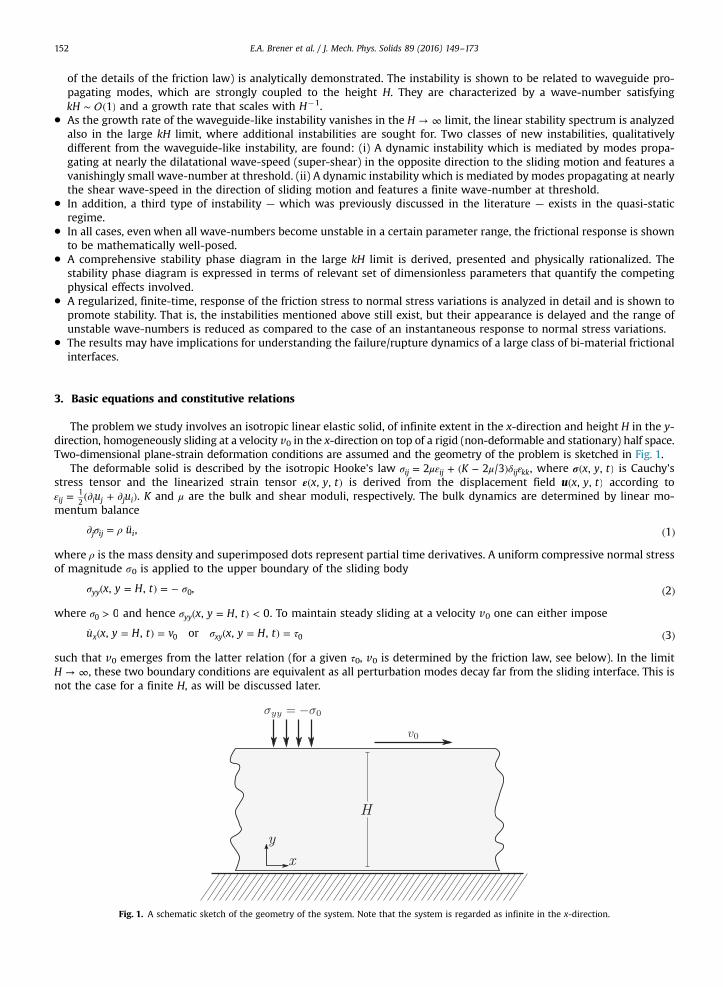
The problem we study involves an isotropic linear elastic solid, of infinite extent in the x-direction and height H in the y-direction, homogeneously sliding at a velocity v0 in the x-direction on top of a rigid (non-deformable and stationary) half space.Two-dimensional plane-strain deformation conditions are assumed and the geometry of the problem is sketched in Fig. 1.

The deformable solid is described by the isotropic Hooke's law σ με μ δ ε= + ( − )K2 2 /3ij ij ij kk, where σ( )x y t, , is Cauchy'sstress tensor and the linearized strain tensor ε( )x y t, , is derived from the displacement field ( )u x y t, , according toε = (∂ + ∂ )u uij i j j i

12

. K and μ are the bulk and shear moduli, respectively. The bulk dynamics are determined by linear mo-mentum balance

σ ρ∂ = ¨ ( )u , 1j ij i

where ρ is the mass density and superimposed dots represent partial time derivatives. A uniform compressive normal stressof magnitude s0 is applied to the upper boundary of the sliding body

σ σ( = ) = − ( )x y H t, , , 2yy 0

where σ > 00 and hence σ ( = ) <x y H t, , 0yy . To maintain steady sliding at a velocity v0 one can either impose

σ τ ( = ) = ( = ) = ( )u x y H t v x y H t, , or , , 3x xy0 0

such that v0 emerges from the latter relation (for a given τ0, v0 is determined by the friction law, see below). In the limit→ ∞H , these two boundary conditions are equivalent as all perturbation modes decay far from the sliding interface. This is

not the case for a finite H, as will be discussed later.

Fig. 1. A schematic sketch of the geometry of the system. Note that the system is regarded as infinite in the x-direction.

E.A. Brener et al. / J. Mech. Phys. Solids 89 (2016) 149–173 153

To complete the formulation of the problem, we need to specify the boundary conditions on the sliding interface at y¼0.First, as the lower body is assumed to be infinitely rigid, we have

( = ) = ( )u x y t, 0, 0. 4y

Note that interfacial opening displacement, ( = ) >u x y t, 0, 0y , is excluded, which is fully justified in the context of thelinearized analysis to be performed below. Eq. (4) is obtained in the limit of large material contrast. In the opposite limit, i.e.for interfaces separating identical materials, the boundary condition reads σ σ( = ) = −x y, 0yy 0 (assuming also symmetricgeometry and anti-symmetric loading). This difference in the interfacial boundary condition is responsible for all of the bi-material effects to be discussed below. The identical materials problem is qualitatively different from the bi-material pro-blem and most of the instabilities we discuss below for the latter problem are expected not to exist for the former.

Next, we should specify a friction law which takes the form of a relation between three interfacial quantities

σ σ τ σ( ) ≡ − ( = ) ( ) ≡ ( = ) ( ) ≡ ( = ) ( )x t x y t x t x y t v x t u x y t, , 0, , , , 0, , , , 0, , 5yy xy x

and possibly a small set of internal state variables (note that in the general case we have( ) ≡ ( = ) − ( = )+ −v x t u x y t u x y t, , 0 , , 0 ,x x . Here ( = ) =−u x y t, 0 , 0x due to the rigid substrate and only ≥y 0 is of interest). Aswas mentioned in Section 1, the class of rate-and-state friction models we consider involves a single internal state variable,which we denote by ϕ( )x t, (the physical meaning of ϕ will be discussed later). Within this constitutive framework, the twodynamical interfacial fields, the friction stress τ( )x t, and ϕ( )x t, , satisfy a coupled set of ordinary differential equations intime (no spatial derivatives are involved) of the form

τ τ σ ϕ ϕ τ σ ϕ = ( ) ⋅ = ( ) ( )F v G v, , , and , , , . 6

Various explicit forms of the functions τ σ ϕ( )F v, , , and τ σ ϕ( )G v, , , will be discussed later (some were already alluded to inSection 1).

Under homogeneous steady-state conditions, when s0 and v0 are controlled at the upper boundary of the sliding body, τ0and ϕ0 are determined from Eq. (6) according to

τ σ ϕ τ σ ϕ( ) = ( ) = ( )F v G v, , , 0 and , , , 0, 70 0 0 0 0 0 0 0

and the steady-state displacement vector field ( )( )u x y t, ,0 satisfies

τμ

σμ

( ) = + ( ) = −+ ( )

( ) ( )u x y t v t y u x y tK

y, , and , ,43

.

8

x y0

00 0 0

We assume >v 00 hereafter. Our goal in the rest of this paper would be to study the linear stability of this solution, forvarious constitutive relations.

4. Linear stability spectrum for standard rate-and-state friction

We consider first the standard rate-and-state friction model in which the friction stress τ depends on the slip velocity v

and a state variable ϕ (Marone, 1998; Baumberger and Caroli, 2006). The latter is of time dimensions and represents the age(or maturity) of contact asperities (Dieterich, 1978; Ruina, 1983; Baumberger and Caroli, 2006). It is directly related to theamount of real contact area at the interface (the “older” the contact, the larger the real contact area is) and hence to thestrength of the interface (Dieterich and Kilgore, 1994; Nakatani, 2001; Nagata et al., 2008; Ben-David et al., 2010). In staticsituations, when v¼0, the age of a contact formed at time t0 is simply ϕ = −t t0. In steady sliding at a velocity v0, thelifetime of a contact of linear size D is ϕ = D v/0 0 (Dieterich, 1978; Teufel and Logan, 1978; Rice and Ruina, 1983; Marone,1998; Nakatani, 2001; Baumberger and Caroli, 2006). D is a memory length scale which plays a central role in this class ofmodels. These two limiting cases are smoothly connected by choosing the function (·)G in Eq. (6) such that (Ruina, 1983; Riceand Ruina, 1983; Marone, 1998; Baumberger and Caroli, 2006)

⎜ ⎟⎛⎝

⎞⎠ϕ τ σ ϕ ϕ˙ = ( ) =

( )G v g

vD

, , , ,9

with ( ) =g 1 0 and ( ) =g 0 1. Furthermore, as sliding reduces the age of the contacts, we typically expect ′( ) <g 1 0.The evolution of τ is assumed to take the form

τ τ σ ϕ τ σ ϕ = ( ) = − ( − ( )) ( )F vT

f v, , ,1

, , 10

where T is a relaxation time scale. For →T 0, which is assumed here (in Section 7 we will consider a finite T), we obtain

τ σ ϕ= ( ) ( )f v, , 11

which completes the definition of the standard rate-and-state friction model.

E.A. Brener et al. / J. Mech. Phys. Solids 89 (2016) 149–173154

Within a linear perturbation approach, the steady-state elastic fields in Eq. (8) and the steady-state of the state variable,ϕ = D v/0 0, are introduced with interfacial (i.e. at y¼0) perturbations proportional to Λ[ − ]t ikxexp , where k is a real wave-number and Λ is a complex growth rate. The ultimate goal then is to find the linear stability spectrum, Λ( )k , and in particularto understand under which conditions R Λ( ) changes sign. R Λ( ) < 0 corresponds to stability as perturbations decay ex-ponentially in time, while R Λ( ) > 0 corresponds to instability as perturbations grow exponentially.

Before we perform this analysis, we would like to gain some physical insight into the structure of the problem. For thataim, we consider Eqs. (5) and (11), and calculate the variation of the latter in the form

δσ δτ σ δ δσ= = − ( )f f , 12xy yy0

where all quantities are evaluated at the interface, y¼0, and the variation is taken relative to the same interfacial field (e.g.the perturbation in the slip δux or slip velocity δv). When all of the terms are evaluated, the above expression becomes animplicit equation for the linear stability spectrum Λ( )k . It is obtained through a balance of three contributions. One con-tribution is δsxy, which is determined from the elastodynamic perturbation problem and is not directly coupled to thefriction coefficient f. Another contribution is proportional to δsyy, which is also determined from the elastodynamic per-turbation problem, but which is multiplied by the friction coefficient f. As this is the only place in the perturbation analysiswhere f appears explicitly, every term that is proportional to f in the expressions to follow, can be physically identified withthe variation of the normal stress syy (and hence with the bi-material effect). Finally, the remaining contribution is de-termined by the variation of the friction coefficient δ ϕ( )f v, , which is affected both by the variation of the slip velocity v andof the state variable ϕ, and is multiplied by the applied normal stress s0. Next, we aim at calculating each of these con-tributions, which are being intentionally presented in some detail.

4.1. Perturbation of the elastodynamic fields

We seek a solution of the linear momentum balance equations (1), coupled to Hooke's law, which is proportional toΛ[ − ]t ikxexp . Consequently, we derive the general solution δ ( )u x y t, , of the problem as a superposition of shear-like and

dilatational-like modes (which lead to an interfacial perturbation proportional to Λ[ − ]t ikxexp ) in the form

⎛⎝⎜

⎞⎠⎟

⎛⎝⎜⎜

⎞⎠⎟⎟

⎛

⎝

⎜⎜⎜⎜⎜

⎞

⎠

⎟⎟⎟⎟⎟

δδ Λ

( )( ) =

−−

[ − ][ − ]

[ ][ ]

[ − ]

( )

u x y tu x y t

k k k k

ik ik ik ik

A k y

A k y

A k y

A k y

t ikx, ,, ,

exp

exp

exp

exp

exp ,

13

x

y

s s

d d

s

d

s

d

1

2

3

4

where{ } = −Ai i 1 4 are yet undetermined amplitudes and we defined Λ Λ( ) ≡ +k k c k, /s s2 2 2 and Λ Λ( ) ≡ +k k c k, /d d

2 2 2 . The shear

and dilatational wave-speeds are μ ρ=c /s and μ ρ= ( + )c K3 4 /3d , respectively. Note that ks d, are in general complex (sinceΛ is complex) and that since we adopt the convention that the branch-cut of the complex square root function lies along thenegative real axis, we have R( ) ≥k 0s d, .

To proceed, we need to impose physically relevant boundary conditions. Recall that at y¼0 we have δ ( = ) =u x y t, 0, 0y

due to the presence of an infinitely rigid substrate. We then focus on the case in which the velocity is controlled at y¼H, i.e. ( = ) =u x y H t v, ,x 0, cf. Eq. (3). Consequently, as both the normal stress syy and tangential displacement ux are controlled at

y¼H, the perturbation satisfies δσ δ( = ) = ( = ) =x y H t u x y H t, , , , 0yy x . Imposing these three boundary conditions on thegeneral solution in Eq. (13) allows us to eliminate the four amplitudes { } = −Ai i 1 4 in favor of a single undetermined amplitude,and express δsxy and δsyy at y¼0 in terms of δux. Using Hooke's law to transform the displacement field into the interfacialstress components, we obtain

δσ μ Λ Λ δ δσ μ Λ δ= − ( ) ( ) = ( ) ( )k k G k H u i kG k H u, , , and , , , 14xy d x yy x1 2

with

ΛΛ

ΛΛ

( ) ≡( )

( ) ( ) −( ) ≡ −

( )( ) ( )

G k HHk c

k k Hk Hk kG k H

G k HHk

, ,coth /

coth tanhand , , 2

, ,coth

,15

d s

d s d s d1

2 2

2 21

and recall that ks d, are both functions of Λ and k. This completes the elastodynamic calculation of δsxy and δsyy at theinterface.

4.2. Perturbation of the friction law

In the next step, we consider the perturbation of the friction law. The calculation is straightforward, yet for completenessand full transparency we explicitly present it here. The variation of ϕ( )f v, with respect to slip velocity perturbations takesthe form

E.A. Brener et al. / J. Mech. Phys. Solids 89 (2016) 149–173 155

⎜ ⎟⎛⎝

⎞⎠δ δϕ

δδ= ∂ + ∂

( )ϕf f fv

v,16v

where all of the derivatives are evaluated at the steady-state values corresponding to v0. As the perturbation in ϕ takes theform δϕ Λ∼ [ − ]t ikxexp , we can use Eq. (9) to obtain

⎜ ⎟ ⎜ ⎟⎛⎝

⎞⎠

⎛⎝

⎞⎠

δϕδ Λ Λ

=′( )

− ′( )= − | ′( )|

+ | ′( )|( )

vg

v gvD

g

v gvD

1

1

1

1,

1700

00

where in the latter we used ′( ) = − | ′( )|g g1 1 because ′( ) <g 1 0. Finally, since ϕ = −d D v/v 0 02, we can relate ∂ϕf to dvf according to

= ∂ − ∂( )

ϕd f fDv

f .18

v v02

Substituting Eqs. (17) and (18) into Eq. (16) and using δ Λδ=v ux, we obtain the final expression for the perturbation of ϕ( )f v,

⎛⎝⎜

⎞⎠⎟δ Λ

ΛΛ δ=

+| ′( )| ∂ +

| ′( )|

( )

fg v

D

fg v

Dd f u

11

.

19

v v x0

0

4.3. The linear stability spectrum and dimensionless parameters

Now that we have calculated the perturbations of δsxy, δsyy and δf in terms of δux, we are ready to derive the linearstability spectrum. For that aim, we substitute Eqs. (14) and (19) into Eq. (12) and eliminate δux to obtain

( )Λ μ Λ Λ μ Λσ Λ

ΛΛ( ) ≡ ( ) ( ) − ( ) +

+| ′( )| ∂ +

| ′( )|=

( )

S k H k k G k H i kf G k Hg v

D

fg v

Dd f, , , , , , ,

11

0.

20

d v v1 20

0

0

This is an implicit expression for Λ( )k , which is in general a multi-valued function with various branches. Analyzing Eq. (20)is the major goal of this paper.

As a first step, we briefly discuss the symmetry properties of Eq. (20). The latter satisfies Λ Λ( − ) = ( )S k H S k H, , , , , where abar denotes complex conjugation. This implies that for each mode with <k 0, there exists another mode with >k 0, whichhas the same growth rate R Λ( ) and an opposite sign frequency I Λ− ( ). Consequently, we have Λ Λ( − ) = ( )k k . These twomodes have the same phase velocity I Λ( ) k/ (because both the numerator and the denominator change sign when → −k k)and they propagate in the same direction. These symmetry properties allow us to assume hereafter >k 0 without loss ofgenerality.

We would now like to discuss the set of dimensionless parameters that control the linear stability problem. In addition tof itself, which is obviously a relevant dimensionless quantity, we define the following three quantities

Δ β γ μσ

≡∂

≡ ≡∂ ( )

d ff

cc c f

, , ,21

v

v

s

d s v0

which involve material/interfacial parameters, interfacial constitutive functions that may depend on the sliding velocity (i.e.dvf and ∂ fv ), and the applied normal stress s0. The first quantity, Δ, is the ratio between the steady-state and the in-stantaneous variation of fwith v (“instantaneous” here means that the slip velocity variation takes place on a time scale overwhich the state variable ϕ does not change appreciably). As such, Δ is a property of the frictional interface. As mentionedabove, frictional interfaces generally exhibit a positive instantaneous response to slip velocity changes (a positive “directeffect”), ∂ >f 0v , which is assumed here. Consequently, the sign of Δ is determined by the sign of dvf, that is, by whetherfriction is steady-state velocity-weakening or velocity-strengthening in a certain range of sliding velocities. While steady-state velocity-weakening is prevalent at small sliding velocities and is very important for rapid slip nucleation (Rice andRuina, 1983; Dieterich, 1992; Ben-Zion, 2008), some frictional interfaces are intrinsically steady-state velocity-strengthening(Noda and Shimamoto, 2009; Ikari et al., 2009, 2013). Moreover, it has been recently argued (Bar-Sinai et al., 2014) that dryfrictional interfaces generically exhibit a crossover from steady-state velocity-weakening, <d f 0v , to velocity-strengthening,

>d f 0v , with increasing v beyond a local minimum. This claim has been supported by a rather extensive set of experimentaldata for a range of materials (Bar-Sinai et al., 2014).

From this perspective, it would be instructive to write Δ using Eq. (18) as

Δ = −∂

∂= −

∂∂ ( )

ϕ ϕD f

v f

f

f1 1 ,

22v v02

log

log

where generically ∂ >ϕf 0 (i.e. frictional interfaces are stronger the older – the more mature – the contact is) and recall thatall derivatives are evaluated at steady-state corresponding to a sliding velocity v0 (i.e. =v v0 and ϕ = D v/0 0). Hence, a

E.A. Brener et al. / J. Mech. Phys. Solids 89 (2016) 149–173156

crossover from Δ < 0 at relatively small v0's to Δ > 0 at higher v0's implies a crossover from ∂ > ∂ϕ f fvlog log to ∂ < ∂ϕ f fvlog log

with increasing v0. While our analysis can be in principle applied to any Δ, the most interesting physical regime correspondsto Δ > 0, i.e. to sliding on a steady-state velocity-strengthening friction branch, where friction appears to be stabilizing andthe destabilization emerges from elastodynamic bi-material and finite size effects (see below). For steady-state velocity-weakening friction, which has been studied quite extensively in the past (Dieterich, 1978; Rice and Ruina, 1983; Marone,1998), we have Δ < 0 and some unstable modes always exist. This instability is of a different physical origin compared to theinstabilities to be discussed below. Physical considerations (Bar-Sinai et al., 2014) indicate that increasing the steady-statesliding velocity v0 along the velocity-strengthening branch is accompanied by either a decrease in ∂ ϕ flog or an increase in∂ fvlog , or both. In the limiting case, ∂ ⪡∂ϕ f fvlog log , we have Δ → 1. Consequently, on the steady-state velocity-strengtheningbranch we have Δ≤ ≤0 1.

The second quantity, β, is the ratio between the shear wave-speed cs and the dilatational wave-speed cd and hence is apurely linear elastic (bulk) quantity. β is only a function of Poisson's ratio ν (in terms of the shear and bulk moduli, we haveν μ μ= ( − ) ( + )K K3 2 / 6 2 ), which for plane-strain conditions takes the form

β νν

= −( − ) ( )

1 22 1

.23

For ordinary materials we have ν≤ ≤0 12(recall that thermodynamics imposes a broader constraint, ν− ≤ ≤1 1

2, but ne-

gative Poisson's ratio materials are excluded from the discussion here), which translates into β≤ ≤0 12.

The third quantity, γ, is the ratio between the elastodynamic quantity μ c/ s — proportional to the so-called radiationdamping factor for sliding (Rice, 1993; Rice et al., 2001; Crupi and Bizzarri, 2013) — and the instantaneous response of thefrictional stress to variations in the sliding velocity, τ σ∂ = ∂ fv v0 . The latter is a product of the externally applied normal stresss0 and ∂ fv . As such, γ quantifies the relative importance of elastodynamics, the applied normal stress and the direct effect(an intrinsic interfacial property). It has been shown that many frictional interfaces are characterized by an instantaneouslinear dependence of f on vlog over some range of slip velocities due to thermally-activated rheology. In this case, ∂ fvlog is apositive constant and ∂ = ∂f f v/v vlog 0 is a decreasing function of v0. Therefore, as v0 increases (for a fixed s0), elastodynamicsbecomes more important and γ increases. Finally, note that as σ > 00 and ∂ >f 0v , we have γ > 0.

In terms of the four independent dimensionless parameters Δ, β, γ and f, the linear stability spectrum in Eq. (20) can berewritten as

Λ μ Λ Λ μ Λ μ Λ λ Λ Δγ λ Λ

( ) = ( ) ( ) − ( ) + ( ) +( ( ) + )

=( )

S k H k k G k H i kf G k Hc

, , , , , , ,1

0,24d

s1 2

where λ Λ Λ( ) ≡ | ′( )|D g v/ 1 0. The shear modulus μ clearly drops as a common factor and then the only dimensional quantitiesleft are k and Λ c/ s, which obviously form a dimensionless combination.

The main goal of most of the remaining parts of this paper is to find the solutions (i.e. roots) of Eq. (24), especially thosewith R Λ( ) > 0. Eq. (24) is a complex equation (both in the complex-variable sense and in the literal sense) which includesbranch-cuts in the complex-plane and is expected to have several solutions Λ( )k . In looking for these solutions, one canfollow various strategies. One strategy would be to numerically search for these solutions. We do not adopt this strategy inthis paper. Rather, we will show that solutions of Eq. (24) are physically related to various elastodynamic solutions and thatthis insight can be used to obtain a variety of analytic results (which are then supported numerically). Below we treatseparately the small and large kH limits of Eq. (24).

5. Analysis of the spectrum in the small kH limit

Our first goal is to analyze the linear stability spectrum in Eq. (24) in the small kH limit, where ∼ ( )kH 1 or smaller. Inthis range of wave-numbers k, perturbations are strongly coupled to the finite boundary at y¼H. The most notable physicalimplication of this is that the elastodynamic solutions in the bulk are non-decaying in the y-direction. Consequently, we willlook for solutions that are related to waveguide-like solutions featuring a propagative wave nature in the x-direction and astanding wave nature in the y-direction.

In general, a 2D wave equation would give rise to a dispersion relation of the form Λ = − ( + )c k kx y2 2 2 2 (c is some wave-

speed). In the presence of a finite boundary at y¼H, some quantization of the wavenumber emerges. In particular, thisquantization implies that in the long wavelength limit ≡ →k k 0x , the dispersion relation results in a cutoff frequencyΛ π= ± icm H/ , with m being a set of numbers (typically integers/half-integers) which are determined by the boundaryconditions. This property will be shown below to have significant implications on the stability problem.

Based on the idea that waveguide-like solutions might be important for the stability problem, we seek now solutions toEq. (24) in the limit →k 0. For that aim, we look first for solutions corresponding to δσ Λ( ) =k, 0xy , which defines the relevantwaveguide dispersion relation Λ ( )kwg . Following Eqs. (14) and (15), solutions of interest correspond to ( ) =Hkcoth 0d , i.e.

E.A. Brener et al. / J. Mech. Phys. Solids 89 (2016) 149–173 157

ΛΛ π Λ Λ

π( ) = + = ± ( + ) ⟹ ≡ ( → ) = ±

( + )

( )Hk k H

ck

i nk

i n cH

,2 1

20

2 12

,25

d wgwg

dwg

d2

22

0

where Λ0 is the waveguide cutoff frequency.Our strategy will be to expand Λ( )S k H, , of Eq. (24), as a function of the two variables k and Λ, to leading order around

Λ Λ( = = )k, 00 . That is, we expand Λ( )S k H, , to linear order in k and in δΛ, Λ Λ δΛ δΛ≃ + + ( )02 , and then set Λ( ) =S k H, , 0 to

obtain δΛ( )k . This procedure is expected to yield a solution that satisfies δΛ( ) ∼k k. In principle, if indeed a solution thatsatisfies R δΛ[ ( )] ∼k k exists (i.e. k¼0 is a regular point where a linear expansion exists), then irrespective of the sign of theproportionality coefficient we have R δΛ[ ( )] >k 0 for either >k 0 or <k 0, implying an instability. In fact, a similar conclusioncan be reached even if the discussion is restricted to >k 0. In this case, if Λ Λ δΛ( ) ≃ + ( )k k0 —with a pure imaginary Λ0 and acomplex δΛ( ) ∼k k — is a solution of Λ( ( ) ) =S k k H, , 0 then the symmetry property Λ Λ( − ) = ( )S k H S k H, , , , implies that

R IΛ δΛ δΛ( ¯ + [ ( )] − [ ( )] − ) =S k i k k H, , 00 . Therefore,

R I R IΛ Λ δΛ δΛ Λ δΛ δΛ( ) ≃ ¯ + [ ( − )] − [ ( − )] = ¯ − [ ( )] + [ ( )] ( )k k i k k i k 260 0

is also a solution of Λ( ( ) ) =S k k H, , 0.We thus conclude, based on the last argument, that if a solution with a complex δΛ( ) ∼k k near Λ0 (purely imaginary)

exists, then actually there exist two solutions with the same I δΛ[ ( )]k and R δΛ[ ( )]k of opposite signs. Both solutions propagatewith the same group velocity I δΛ[ ]d dk/ , but one is stable (R δΛ[ ( )] <k 0) and the other is unstable (R δΛ[ ( )] >k 0). This leads tothe quite remarkable conclusion that steady-state sliding along (strongly) bi-material frictional interfaces in this broad classof constitutive models is universally unstable.

To fully establish this important result, we derive it by an explicit calculation. To that aim, as explained above, we need toexpand Λ( )S k H, , of Eq. (24) to leading order around Λ Λ( = = )k, 00 . This is done in detail in Appendix A, but the essence isgiven here. The contribution related to δsyy in Eq. (24) is proportional to both Λ( )G k H, ,2 and k; the former diverges in thelimit Λ Λ( ) → ( )k, , 00 , while the latter clearly vanishes. In total, the term proportional to δsyy approaches the finite limit

Λβ Λ δΛ

( ) ≃ ±( | | ) ( )

ikfG k Hfc k

H H c, ,

tan /,

27s

s2 2

0

where the 7 corresponds to Λ Λ= ± | |i0 0 . This leads to the non-trivial situation in which the leading order contributioninvolves the ratio of δΛ and k.

Consequently, the contributions related to δsxy and δf can be taken, albeit with some care, to zeroth order, yielding (seeAppendix A for details)

Λ ΛΛ

Λ( ) ( ) ≃

| |( | | ) ( )

k k G k Hc H c

, , ,tan /

,28d

s s1

0

0

⎛⎝⎜⎜

⎞⎠⎟⎟σ δ

Λ λ Δγ λ

Λγ

λ Δ Δ λλ

≃+

( + )=

| | −| |( − ) ± ( + | | )+ | | ( )

fc c

i1

11

,29s s

00 0

0

0 0 02

02

-0.1

0

0.1

0.2

0 1 2 3

Re(Λ

) H/c

s

H k

n=0

n=1

n=2

γf=0.9γf=0.6γf=0.3

0

0.05

0.1

0.15

0.2

0 0.5 1 1.5 2

Re(Λ

) H/c

s

H k

H~=0.5H~=5

H~=50H~=500

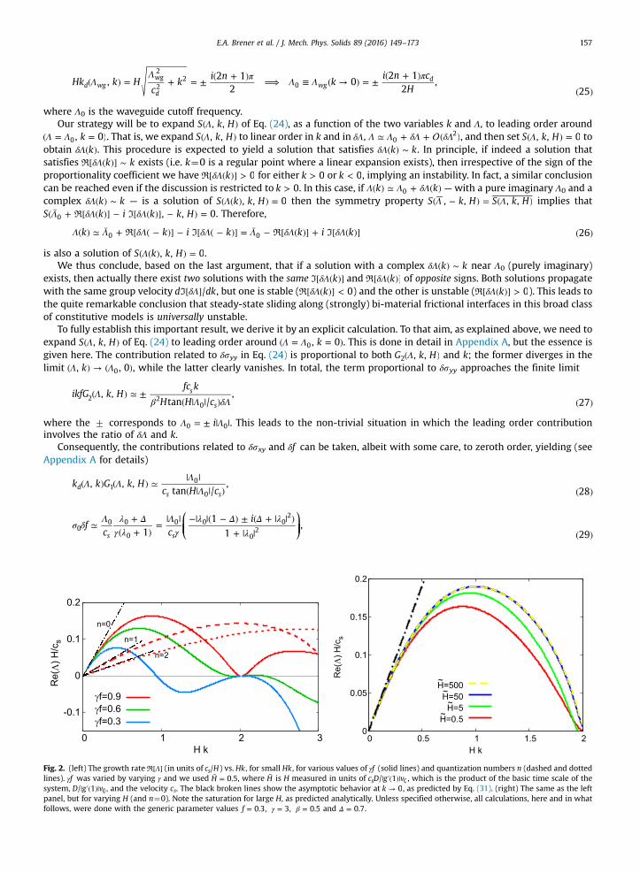
Fig. 2. (left) The growth rateR Λ[ ] (in units of c H/s ) vs. Hk, for small Hk , for various values of γf (solid lines) and quantization numbers n (dashed and dottedlines). γf was varied by varying γ and we used ˜ =H 0.5, where H is H measured in units of | ′( )|c D g v/ 1s 0, which is the product of the basic time scale of thesystem, | ′( )|D g v/ 1 0, and the velocity cs. The black broken lines show the asymptotic behavior at →k 0, as predicted by Eq. (31). (right) The same as the leftpanel, but for varying H (and n¼0). Note the saturation for large H, as predicted analytically. Unless specified otherwise, all calculations, here and in whatfollows, were done with the generic parameter values γ β= = =f 0.3, 3, 0.5 and Δ = 0.7.

E.A. Brener et al. / J. Mech. Phys. Solids 89 (2016) 149–173158

where λ Λ≡ | ′( )|D g v/ 10 0 0. Collecting all three contributions we end up with

ΛΛ

Λ β Λ δΛΛ λ Δ

γ λ( ) ≃

| |( | | )

±( | | )

++

( + )=

( )S k H

c H c

fc k

H H c c, ,

tan / tan / 10.

30s s

s

s s

0

02

0

0 0

0

Eq. (30) clearly establishes a linear relation between δΛ and k. Extracting Λ Λ δΛ( ) = + ( )k k0 by solving Eq. (30), we obtain

R

⎡⎣⎢

⎤⎦⎥

⎛⎝⎜⎜

⎞⎠⎟⎟

⎛⎝⎜⎜

⎞⎠⎟⎟

Λβ Λ

ΛΛ

Λγ

λ Δλ

ΛΛ

Λγ

λ Δλ

Λγ

Δ λλ

( ) ≃ ∓( | | )

| |( | | )

−| | | |( − )

+ | |

| |( | | )

−| | | |( − )

+ | |+

| | + | |+ | |

+ ( )

( )

fc k

H H c c H c c

c H c c c

ktan / tan /

11

tan /1

1 1

,

31

s

s s s s

s s s s

20

0

0

0 0

02

0

0

0 0

02

20 0

2

02

22

where I δΛ[ ] can be easily obtained as well and is independent of the sign of I Λ[ ]0 . Eq. (31) has precisely the predictedstructure, i.e. there are two solutions for Λ in the small >k 0 limit, whose real parts have opposite signs. Consequently, asolution with R Λ[ ] > 0 always exists, i.e. the system is universally unstable.

While Eq. (31) can be somewhat simplified, it is retained in this form so that the physical origin of the various terms willremain transparent. Note that in the particular case of β = 1/2 (which will be used in some of the numerical calculationsbelow), a significant simplification is obtained, leading to an unstable branch R Λ π( ) ≃ [( + ) ] + ( )fkc n k4 / 2 1s

2 (some careshould be taken when obtaining this result as a naive substitution of β = 1/2 in Eq. (31) results in some apparently divergentcontributions). The analytic result for the small k behavior of the growth rate R Λ[ ] presented in Eq. (31), which is one of themain results of this paper, is verified in Fig. 2 for the few first n's by a direct numerical solution of the linear stabilityspectrum in Eq. (24). The numerical solution of the spectrum shows that the most unstable mode satisfies ∼ ( )kH 1 , whereR Λ[ ] attains its first maximum (corresponding to the n¼0 solution). This can be analytically obtained by calculating the

( )k2 correction to Eq. (31), though the calculation is lengthy.We thus conclude that the finite size H of the sliding system has significant implications for its stability, in particular it

implies the existence of an instability with a wavelength determined by H. This instability should be relevant to a broadrange of systems, for example an elastic brake pad sliding over a much stiffer substrate, for which recent numerical resultsdemonstrated dominant instability modes directly related to the intrinsic vibrational modes of the pad (Behrendt et al.,2011; Meziane et al., 2007). The universal existence of this finite H instability does not immediately mean that it will beindeed observed since other instabilities, which do not necessarily satisfy ∼ ( )kH 1 , might exist and feature a larger growthrate (when several instabilities coexist, the one with the largest growth rate will be the dominant one).

To further clarify this point, we consider large, but finite, H in Eq. (31). In this limit, by counting powers of H andsubstituting k∼H�1 for the fastest growing mode, we obtain for the latter R Λ[ ] ∝ fc H/s . This scaling is verified numerically inFig. 2 (right panel). This result shows that this instability depends on the presence of friction, but not very much on thedetails of the friction law (e.g. the length scale D does not play a dominant role), and that the growth rate of the instabilitydecreases with increasing H. This raises the question of whether in the large H limit there exist other instabilities with alarger growth rates, which will be addressed in the rest of the paper.

It is important to note that while we highlight the role of the finite size H in relation to the universal instability en-capsulated in the growth rate in Eq. (31), we should stress that the bi-material effect remains an essential physical in-gredient driving this instability. This is evident from the observation that R Λ[ ] is proportional to f in Eq. (31), where — asexplained in Section 4— the latter is a clear signature of the variation of the normal stress with slip, which is associated withthe bi-material effect. We thus expect that this universal instability does not exist for frictional interfaces separatingidentical materials. The effect of finite material contrast will be addressed in a separate report.

Before we discuss the large H limit, → ∞kH , we would like to note another interesting implication of the finite systemsize H. For infinite systems, → ∞H , there is an equivalence between velocity-controlled and stress-controlled externalboundary conditions (cf. Eq. (3)) because perturbations decay exponentially away from the interface in the y-direction. Thisequivalence breaks down for a finite H. The analysis above focussed on velocity-controlled boundary conditions. In Ap-pendix B, we consider also stress-controlled boundary conditions and explicitly demonstrate the inequivalence of the twotypes of boundary conditions for finite size systems. The differences, though, are quantitative in nature and the genericinstabilities discussed above remain qualitatively unchanged.

Finally, we would like to note that there can be solutions to Eq. (24) in the small kH limit other than Eq. (31). We are notlooking for them here because the result in Eq. (31) already shows that the system is always unstable. In addition, we expectthe decay of the growth rate R Λ[ ] with H to be a generic property of unstable solutions of Eq. (24) in the small kH limit.Consequently, we focus next on the large kH limit, looking for qualitatively different unstable solutions.

6. Analysis of the spectrum in the → ∞kH limit

After analyzing the linear stability spectrum of Eq. (24) in the small kH limit, our goal now is to provide a thoroughanalysis of the opposite limit, → ∞kH . The length H enters the problem through the elasticity relations in Eq. (14) and moreprecisely through the functions G1,2 in Eq. (15). Taking the → ∞kH limit in Eq. (15), which amounts to taking the arguments

E.A. Brener et al. / J. Mech. Phys. Solids 89 (2016) 149–173 159

of (·)coth and (·)tanh to be arbitrarily large, we obtain

Λ Λ ΛΛ Λ

Λ Λ Λ

( → ∞) → ( ) =[ ( ) ( ) − ]

( → ∞) → ( ) = − ( ) ( )

G k H g kc k k k k k

G k H g k g k

, , ,, ,

,

, , , 2 , , 32

s s d1 1

2

2 2

2 2 1

which should be used in Eq. (24). The friction part is of course independent of H.To further simplify the analysis of the spectrum in this limit, we define an auxiliary (and dimensionless) complex variable

z that relates the spatial and temporal properties of perturbations according to

Λ≡ −( )

zikc

.33s

Defining the dimensionless wave-number as ≡ | ′( )|q c Dk g v/ 1s 0, and recalling that we already defined above the di-mensionless (complex) growth rate as λ Λ≡ | ′( )|D g v/ 1 0, Eq. (33) can be cast as λ = − iqz . With these definitions, Eq. (24) canbe rewritten as

⎡⎣⎢

⎤⎦⎥γ β β β Δ( ) ≡ ( − ) − ( ) − ( ) − ( − ) = ( )s z q iqz z g z ifg z iz iqz, 1 1 , , 0, 34

2 21 2

where

ββ

β β( ) =− − −

( ) = − ( )( )

g zz

z zg z g z,

1 1 1and , 2 , .

351

2

2 2 2 2 1

As before, Eq. (34) is an implicit expression for the explicit spectrum z(q), which depends on the four dimensionlessparameters Δ, β, γ and f. Note also that due to algebraic manipulations, Eq. (34) no more follows the structure of Eq. (12)(which is preserved in Eqs. (20) and (24)), rather the terms are mixed to some extent. Later on, when discussing some of thephysics behind our results, we will reinterpret them in terms of Eq. (12). Due to the appearance of the complex square rootfunction in the above expressions, Eq. (34) is understood as having a branch-cut on the real axis along | | >z 1 (there is also a

branch-cut on the real axis along β| | >z 1/ associated with β− z1 2 2 . Combinations of − z1 2 and β− z1 2 2 , as in Eq. (34),may have more complicated branch-cut structures). The existence of these branch-cuts has implications that will be dis-cussed later. Finally, in analyzing Eq. (34) we assume that the dimensionless wave-number q — and hence the dimensionalwave-number k — spans the whole interval < < ∞q0 . The small wave-numbers limit, →q 0, is understood to imply

⪡| ′( )|Dk g v c1 / s0 while maintaining ⪢kH 1. This can always be guaranteed by having a sufficiently large H.In the next parts of this section we present an extensive analysis of the linear stability spectrum in Eq. (34). As in Section

5, we will establish relations between the unstable solutions of Eq. (34) and various elastodynamic solutions and use thisinsight to derive analytic results that will shed light on the underlying physics. In Section 6.1 we show that there existunstable solutions related to dilatational waves propagating in the direction opposite to the sliding motion. In Section 6.2we show that there exist another class of unstable solutions which are related to shear waves propagating in the directionsliding motion. In Section 6.3 we briefly review a qualitatively different class of solutions, which are not elastodynamic innature, but rather quasi-static (Rice et al., 2001). In Section 6.4 we present a comprehensive stability phase diagram, whichputs together all three classes of solutions of the linear stability spectrum in Eq. (34). While we do not provide a mathe-matical proof that other classes of solutions do not exist, we suspect that our analysis is exhaustive.

6.1. Dilatational wave dominated instability

In the spirit of Section 5, we will look for solutions of Eq. (34) that are related to propagating wave solutions. In particular,we note that the linear stability spectrum of Eq. (34) significantly simplifies when β=z 1/ , for which β− z1 2 2 vanishes.Physically, the latter corresponds to δσ = 0xy , where Λ( ) =k k, 0d and Λ( )g k,1 is finite (cf. Eq. (14) with g1 replacing G1), i.e. tofrictionless boundary conditions. Substituting β=z 1/ in Eq. (34) and taking the limit →q 0, we immediately observe that itis a solution if γ β Δ β( − ) =f 1/ 2 /2 . As will be shown soon, the latter is an exact stability condition for the emergence ofunstable solutions located near β=z 1/ in the complex z-plane. Recall that a real z is equivalent to R Λ( ) = 0, which isprecisely where solutions change from growing (R Λ( ) > 0) to decaying (R Λ( ) < 0) in time.

β=z 1/ corresponds to the dispersion relation for dilatational waves, Λ = − ic kd (i.e. frictionless boundary conditions,δσ = 0xy ), which means that instability modes located near β=z 1/ in the complex-plane travel at nearly the dilatationalwave-speed in the direction opposite to the sliding direction. The direction of propagation is a result of the minus sign in theabove dispersion relation. It is important to stress in this context that while β→ −z 1/ also corresponds to a dilatationalwave (δσ = 0xy ), it is not a solution of Eq. (34). That is, friction in the presence of homogeneous sliding breaks the directionalsymmetry of dilatational waves. The fact that Λ vanishes in the limit →k 0 marks a crucial difference between the analysis tobe performed here and the one in Section 5, where the finite system size H implied a finite cutoff frequency Λ Λ→ 0 in thelimit →k 0.

Following this simplified analysis, which indicates that some unstable solutions might be located near β=z 1/ in the

E.A. Brener et al. / J. Mech. Phys. Solids 89 (2016) 149–173160

complex z-plane, we aim at obtaining analytic results for the spectrum by a systematic expansion around this point. That is,we are interested in obtaining a systematic expansion of the form β δ= +z z1/ , where δz is a small complex number (i.e.δ| |⪡z 1) whose imaginary part determines the stability of sliding (I δ( ) >z 0 implies instability and I δ( ) <z 0 implies stability).This should be done carefully, though, since β=z 1/ is a branch-point, where a Laurent expansion does not exist.

To address this issue, let us briefly discuss one of the physical implications of being close to β=z 1/ . First, note that thereal part of kd in the elastodynamic solution in Eqs. (13) controls the decay length in the y-direction (ks plays a similar role,but is not discussed here. Note also that →A 03,4 in the → ∞H limit considered here, which ensures the proper decay ofsolutions sufficiently away from the interface.). Then, expressing kd in terms of z, β= −k k z1d

2 2 , we observe that kdvanishes as β→z 1/ , i.e. there is no decay in the y-direction in this case, and the proximity to β=z 1/ actually controls thesmallness of kd (for a given wave-number k). Therefore, we define a complex number κ β≡ − z1d

2 2 such that κ=k kd d,where κ| |⪡1d .

With this definition of smallness, we go back to our original motivation to derive a systematic expansion around β=z 1/and express z in terms of κd as

κβ

βκ

βκ=

−≃ − + ( )

( )z

11/

2.

36d d

d

2 24

The latter expression has the desired form β δ= +z z1/ and our next goal is to estimate κd itself from the linear stabilityspectrum in Eq. (34). To do this, we need to rewrite the spectrum in terms of the new independent variable κd. In theproximity of β=z 1/ , the functions ( )g z1 and ( )g z2 in Eq. (35) can be written in terms of κd as follows

κ β

κ βκ κ^ ( ) ≃

∓ −^ ( ) ≃ − ^ ( )

( )∓ ∓ ∓g

ig g

1/

1 1/ 1and 2 ,

37d

d

d d1

2

2 2 1

where the minus sign corresponds to the stable branch (I( ) <z 0) and the plus sign to the unstable branch (I( ) >z 0). This

emerges from the limit β− − → ∓ −z i1 1/ 12 2 as β→z 1/ , where the different signs correspond to taking the limit from

the two sides of the branch-cut (I δ( ) → ∓z 0 ). The main advantage of Eqs. (37) is that κ^ ( )∓

g d1 and κ^ ( )∓

g d2 are analytic such that a

Laurent expansion around κ = 0d exists.2

Using Eqs. (37), we can rewrite the linear stability spectrum in Eq. (34) in terms of κd as

⎡⎣ ⎤⎦κ γ β κ κ κ β Δ β( ) ≃ ( − ) ^ ( ) − ^ ( ) − ( − ) = ( )∓ ∓s q iq g if g i iq, 1 / / / 0, 38d d d d1 2

where we set β=z 1/ . We then linearize the following κd-dependent quantities

κ κ β κ κ β κ β κ^ ( ) ≃ + ( ) ^ ( ) ≃ − ( ± − ) + ( ) ( )∓ ∓k g g i/ , 2 1/ 1 1/ 1 , 39d d d d d d d1

2 22

2 2 2

substitute them into Eq. (38) and solve the resulting linear equation for κd, obtaining

( ( )( )( ) ( )

κγ β β Δ β β

γ β β β≃

− − + −

− ) ∓ − ( )

if iq i iq

iq f

1 / 2 1/ / /

1 / 1 1/ 1 /.

40d

2

2 2

Substituting the latter in Eq. (36), we can calculate the dimensionless growth rate R Iλ( ) = ( )q z in the form

R

⎛

⎝

⎜⎜⎜⎜

⎡⎣ ⎤⎦⎞

⎠

⎟⎟⎟⎟( )( )

( )λ Δ

γ β β β γ β β Δ

γ β β( ) ≃ ( − )

− − + ( − ) −

+ ∓ − ( )

qf q f

q f1

1/ 2 1 / 1/ 2

/ 1 1 1/ 1,

41

22 2 2 2

2 2 2 2 22

where, as before, the stable solution corresponds to the minus sign and unstable one to the plus sign. This analytic pre-diction is one of the major results of this paper. It is important to stress that unlike the growth rate in Eq. (31), which wasobtained by a small wave-numbers expansion, the growth rate in Eq. (41) was obtained by an expansion in the complexplane near β=z 1/ . Consequently, it is valid — as will be explicitly demonstrated below — for any wave-number q.

A lot of analytic insight can be gained from Eq. (41). First, note that the growth rateR λ( ) in Eq. (41) is continuous, but notdifferentiable at the transition from the stable to unstable branches as a function of q (i.e. it has a kink due to the existence ofa branch-cut in the equation for the spectrum). Then, we see that unstable modes appear in the long wavelength regime,

< < ( )q q0 cd , where the critical wave-number ( )qc

d is simply obtained from the condition R λ( ) = 0.

2 We note in passing that we could do the whole analysis with δz instead of κd, invoking the leading term δ∼ z in a fractional power series. The tworoutes are equivalent when identifying κ β δ≃ − z2d , which is precisely what Eq. (36) states.

E.A. Brener et al. / J. Mech. Phys. Solids 89 (2016) 149–173 161

β γ β β Δγ β β

≃ ( − ) −− ( − ) ( )

( )qf

f1/ 2

1 1/ 2.

42cd

2

2

The instability threshold is obtained by taking the limit →( )q 0cd (i.e. the instability does not occur at a finite wavelength)

γ Δβ β

=( − ) ( )

f1/ 2

,432

which is identical to the one derived at the beginning of this section. When the left-hand-side is smaller than the right-hand-side, there exist no unstable modes, i.e. the regime < < ( )q q0 c

d shrinks to zero and R λ( ) is always negative. In theopposite case, when the left-hand-side is larger than the right-hand-side, a finite range of unstable modes emerges. Asimple calculation shows that the threshold condition actually emerges from the numerator of I κ( )d in Eq. (40), and inparticular from its q-independent part (since the threshold condition corresponds to the limit of vanishing wave-number q).

Let us discuss the physics embodied in Eq. (43). For that aim, recall the definitions of γ and Δ in Eq. (21) and substitutethem in Eq. (43) to obtain

μ β β σ( − ) =( )

fc

d f1/ 2 .44s

v2

0

A first observation is that this instability threshold is independent of ∂ fv . Put differently, as far as the threshold is concerned,the distinction between dv f and ∂ fv is irrelevant as if the friction law is only rate-dependent, f(v). This can be understood asfollows; the right-hand-side of Eq. (44) corresponds to the σ δf0 term (variation of the friction law) in Eq. (12). Near thresholdwe have Λ ∼ − →ik 0, which can be substituted in the expression for δf in Eq. (19). We observe that the term proportional to∂ fv scales as k2, while the one proportional to dv f scales as k and hence the latter dominates the former. Consequently, wehave δ ∼f d fv , independent of ∂ fv .

Another aspect of Eq. (44) which is worth noting concerns the left-hand-side, which is proportional to f and hencecorresponds to the fδsyy term in Eq. (12). Indeed, δsyy in Eq. (14) scales as k, while δsxy is higher order in k and hencenegligible. Moreover, we observe that δsyy is proportional to the so-called radiation damping factor for sliding (Rice, 1993;Rice et al., 2001; Crupi and Bizzarri, 2013), μ c/ s, which essentially follows from dimensional considerations in the elasto-dynamic regime. To conclude, the present discussion shows that Eq. (43) is actually of the form σ δσ∼d f fv yy0 , i.e. the onset ofinstability is controlled by a balance between the stabilizing steady-state velocity-strengthening friction, dvf, and the de-stabilizing elastodynamic bi-material effect, δsyy.

Next, we consider the analytic prediction for R Λ( ) in the limit → ∞k (or in dimensionless units, R λ( ) in the limit → ∞q ).By counting powers in Eq. (41) we observe that in the limit → ∞q , R λ( ) approaches a constant whose sign is determined bythe sign of γ β β( − ) −f 1/ 2 12 . If γ β β( − ) <f 1/ 2 12 , then the constant is negative. This does not immediately imply stabilitybecause, following the discussion above, a finite range of unstable modes emerges if Δ γ β β< ( − ) <f 1/ 2 12 . If, on the otherhand, we have

γ β β( − ) > ( )f 1/ 2 1, 452

then the constant is positive, which implies that all wave-numbers are unstable. Indeed, Eq. (42) shows that the criticalwave-number ( )qc

d diverges in the limit γ β β( − ) →f 1/ 2 12 .We have thus seen that when elastodynamic effects become sufficiently strong, i.e. when the combination γf becomes

sufficiently large, all wave-numbers are unstable. This observation raises the issue of ill-posedness, which has been quiteextensively discussed in the literature recently (Renardy, 1992; Adams, 1995; Martins and Simões, 1995; Martins et al., 1995;Simões and Martins, 1998; Ranjith and Rice, 2001). Ill-posedness is a stronger condition than instability for all

-2x10-4

0

2x10-4

4x10-4

0 0.5 1 1.5 2 2.5 3

Re(λ)

q

γf=0.6γf=0.9γf=0.96γf=1.2

1.998

1.999

2

2.001

2.002

2.003

0 0.5 1 1.5 2 2.5 3

Re(

z)

q

γf=0.6γf=0.9γf=0.96γf=1.2

Fig. 3. (left) The dimensionless growth rate R Iλ( ) = ( )q z vs. the dimensionless wave-number q for various γf 's (γf was changed by changing γ). The solidlines show the numerical solution of the linear stability spectrum in Eq. (34) for both the stable (R λ( ) < 0) and unstable (R λ( ) > 0, when it exists) branches.The dotted lines correspond to the analytical prediction of Eq. (41). A very good quantitative agreement between the analytic prediction and the directnumerical solution is demonstrated (see text for more details). The discontinuities (gaps) observed in the full numerical solution are discussed in AppendixC. (right) R( )z vs. the wave-number q. The parameters used are β= =f 0.3, 0.5 and Δ = 0.7.

E.A. Brener et al. / J. Mech. Phys. Solids 89 (2016) 149–173162

wave-numbers, i.e. a problem can feature unstable modes at all wave-numbers but still be mathematically well-posed, andis defined as follows; consider the perturbation of any relevant interfacial field in the linear stability problem, e.g. the slipvelocity field δv, and express it as an integral over all wave-numbers

∫δ Λ( ) ∼ ( ) [ − ] [ ( ) ] ( )−∞

∞v x t a k ikx k t dk, exp exp , 46

where a(k) is the amplitude of the kth mode. If this integral fails to converge, the problem is regarded as mathematically ill-posed.

An important example in this context (Renardy, 1992; Adams, 1995; Martins and Simões, 1995; Martins et al., 1995;Simões and Martins, 1998; Ranjith and Rice, 2001) is sliding along a bi-material interface described by Coulomb friction,τ σ= f (where f is a constant). In this case,R Λ( ( )) ∼ | |k k (with a positive prefactor) and the integral in Eq. (46) fails to convergefor any ≠x 0 at any finite time, unless a(k) decays exponentially or stronger with | |k . The problem can be made well-posed ifin response to normal stress variations, τ σ= f is approached over a finite time scale (Ranjith and Rice, 2001). In our problem,within the standard rate-and-state friction framework, we saw above that there exists a range of parameters in which allwave-numbers are unstable. Yet, in this case R Λ( ( ))k approaches a constant as → ∞k , in which case the integral in Eq. (46)converges. Therefore, we conclude that the response of infinite-contrast bi-material interfaces described by standard rate-and-state friction laws is mathematically well-posed.

We are now in a position to quantitatively compare the analytic predictions derived from Eq. (41) to a direct numericalsolution of the linear stability spectrum in Eq. (34). The results are shown in Fig. 3. On the left panel,R Iλ( ) = ( )q z is shown asa function of q for various γf 's and fixed representative values of Δ, f and β.

All in all, Fig. 3 demonstrates a good quantitative agreement between the analytic prediction and the full numericalsolution over a significant range of parameters and wave-numbers. In particular, Eq. (43) predicts (for the chosen β) that theonset of instability takes place at γ =f 0.7, which is precisely what is observed. Furthermore, the onset of instability appearsat →k 0, as predicted. The critical wave-number ( )qc

d , predicted in Eq. (42), is quantitatively verified for several sets ofparameters above threshold. Finally, the shape of the unstable spectrum, including the constant asymptote as → ∞q , isquantitatively verified.

The only interesting deviation of the analytic prediction of Eq. (41) from the full numerical solution in the left panel ofFig. 3 is that the latter exhibits a discontinuity (a gap) at the transition from the unstable to the stable part of the solution,while the former is continuous but rather exhibits a discontinuous derivative. This results in a shift of the stable part of thespectrumwhen an unstable range of wave-numbers exists. The origin of the gap in the spectrum is explained in Appendix C.On the right panel of Fig. 3,R( )z is shown as a function of q for both the numerical solution of Eq. (34) and the real part of Eq.(36) (together with Eq. (40)). The figure demonstrates, again, a good quantitative agreement between the analytic predictionand the exact numerical solution. Furthermore, the two panels of Fig. 3 show that indeed I R Rλ β( ) = ( ) ⪡ ( ) ≃z q z/ 1/ , asexpected for solutions located near β=z 1/ . In particular, note that solutions remain close to β=z 1/ in the complex-planefor every wave-number in this class of solutions.

With this we complete the discussion of the dilatational wave dominated instability, which corresponds to unstablemodes of predominantly dilatational wave nature propagating in the direction opposite to the sliding direction (corre-sponding to solutions near β=z 1/ ). In the next subsection we discuss a distinct class of unstable solutions of the linearstability spectrum in Eq. (34).

0

2x10-4

4x10-4

6x10-4

0 0.05 0.1 0.15 0.2 0.25

Re(λ)

q

dilatationalwave

instabilityshearwave

instability

Δ=0.05Δ=0.02Δ=0.01

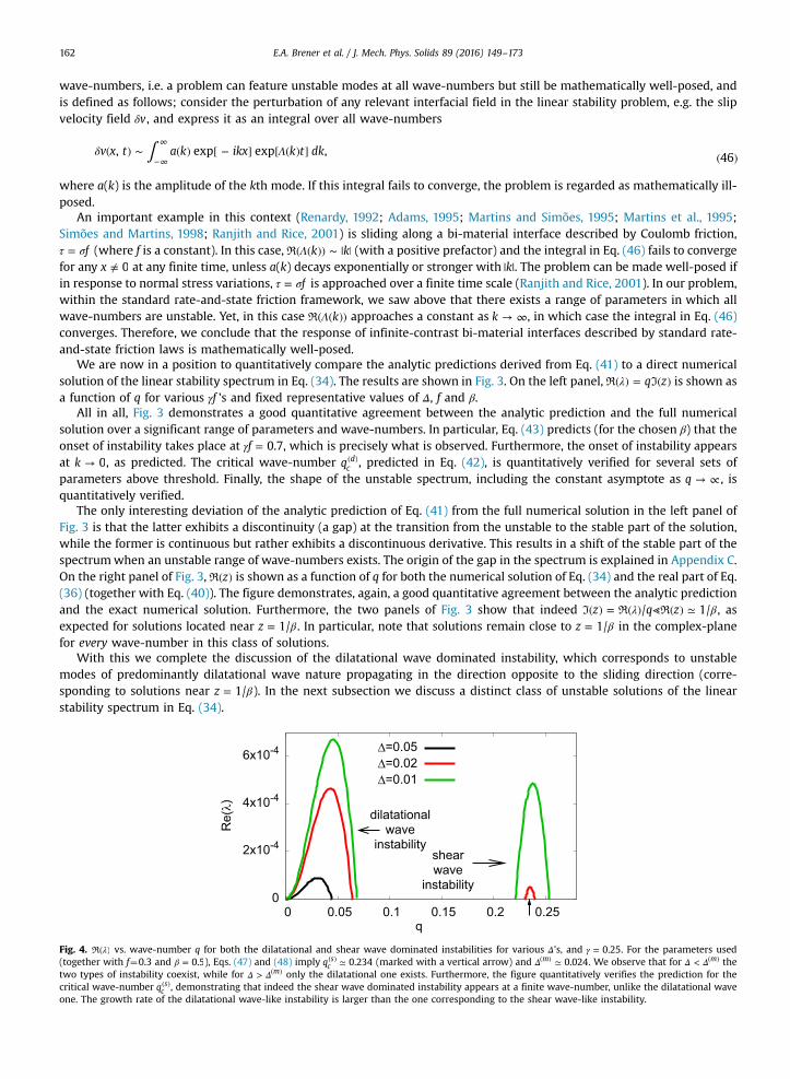
Fig. 4. R λ( ) vs. wave-number q for both the dilatational and shear wave dominated instabilities for various Δ's, and γ = 0.25. For the parameters used(together with f¼0.3 and β = 0.5), Eqs. (47) and (48) imply ≃( )q 0.234c

s (marked with a vertical arrow) and Δ ≃( ) 0.024m . We observe that for Δ Δ< ( )m thetwo types of instability coexist, while for Δ Δ> ( )m only the dilatational one exists. Furthermore, the figure quantitatively verifies the prediction for thecritical wave-number ( )qc

s , demonstrating that indeed the shear wave dominated instability appears at a finite wave-number, unlike the dilatational waveone. The growth rate of the dilatational wave-like instability is larger than the one corresponding to the shear wave-like instability.

E.A. Brener et al. / J. Mech. Phys. Solids 89 (2016) 149–173 163

6.2. Shear wave dominated instability

Inspired by the discussion in the previous subsection, we look here for another class of unstable solutions. This time wefocus on the zeros of − z1 2 , in particular on solutions located near = −z 1 in the complex-plane. As will be shown below,these instability modes are of shear wave-like nature, propagating with a phase velocity close to cs in the sliding direction.

To see how this rigorously emerges, we set = −z 1 in Eq. (34) (which corresponds to R Λ( ) = 0, i.e. to the threshold ofinstability) and separate the real and imaginary parts to obtain

γ βγ

Δ γ γ βγ

=−

−= − ( ) ( − )

( − ) ( )( )q

ff

ff f

11

and1

1,

47cs

2 2 2

2

where ( )qcs is the critical (dimensionless) wave-number at threshold and the second relation is the onset of instability

condition (an instability occurs when the left-hand-side is smaller than the right-hand-side). This is an exact result. Unlikethe dilatational wave dominated instability, which featured a vanishing critical wave-number at threshold, →( )q 0c

d , theshear wave dominated instability takes place at a finite wave-number (above threshold, a finite range of unstable q'semerges around ( )qc

s , cf. Fig. 4). = −z 1 corresponds to the dispersion relation for shear waves, Λ = ic ks , which means that thisinstability is mediated by modes propagating at nearly the shear wave-speed in the direction of sliding. The propagationdirection is determined by the positive sign in the last expression. It is important to stress in this context that z¼1 is not asolution of Eq. (34), again demonstrating the symmetry breaking induced by frictional sliding.

The dilatational wave dominated instability exists for all physically relevant values of Δ, i.e. for Δ≤ ≤0 1. Is it true also forthe shear wave dominated instability? To address this question, we interpret Δ in Eq. (47) as a function of Γ γ≡ f , para-meterized by β and f. Δ Γ( ) is a non-monotonic function which attains a maximum at

Δβ β β

=( − ) + − ( − )( − + )

( )( ) f f

f

2 1 2 1 1.

48m

2 2 2 2 2

2

For realistic values of the friction coefficient f (i.e. ∼ −f 0.2 0.75), we have Δ ⪡( ) 1m , which shows that the shear wavedominated instability is characterized by a small Δ. Furthermore, Δ Γ( ) in Eq. (47) vanishes at Γ β= ( − + )f f/ 12 2 2 , which isalso typically small due to the smallness of f2. In fact, if we assume a small Γ and invoke a parabolic approximation for Δ Γ( )in Eq. (47), we obtain for the maximum Δ β≃ [ ( − )]( ) f / 4 1m 2 2 , which is just the leading contribution in the expansion of Eq.(48) in terms of f2. We thus conclude that the shear wave dominated instability is localized in a relatively small region nearthe origin in the Δ Γ– plane.

One implication of the above discussion is that since in the stability boundary of the dilatational wave dominated in-stability Δ increases linearly with Γ γ= f , cf. Eq. (43), the shear and dilatational waves instabilities coexist only in a relativelysmall range of Δ's, Δ Δ< < ( )0 m . To explicitly demonstrate this, R λ( ) is plotted vs. q in Fig. 4 for the two types of instabilitiesand various small Δ's. We observe that indeed the two instabilities coexist for Δ Δ< < ( )0 m , but only the dilatational oneexists for Δ Δ> ( )m (see figure caption for details), and that the growth rate of the dilatational instability is larger than that ofthe shear one. Furthermore, we see that indeed the dilatational wave dominated instability appears at a vanishing wave-number, while the shear wave dominated instability appears at a finite wave-number. The results for the shear wavedominated instability presented in Fig. 4 were obtained numerically. We could have followed a similar procedure to the onetaken in great detail in Section 6.1 and derive analytic results by systematically expanding around = −z 1 in the complex-plane. In order not to further complicate the presentation, we do not present this analysis here, but rather present numericaldemonstrations of the main physical points.

The analysis of the spectrum in the large kH limit presented so far has revealed two classes of elastodynamic-controlledunstable modes, one mediated by dilatational wave-like modes propagating in the direction opposite to the sliding motion(corresponding to solutions near β=z 1/ ) and one mediated by shear wave-like modes propagating in the direction ofsliding (corresponding to solutions near = −z 1). Related observations on the directionality of unstable modes and rupturealong bi-material frictional interfaces have been previously made, see for example Ranjith and Rice (2001), Cochard and Rice(2000), Adams (2000), Weertman (1980), Andrews and Ben-Zion (1997), Ben-Zion and Huang (2002), Adams (1995), Adams(1998), Harris and Day (1997), Xia et al. (2004), and Ampuero and Ben-Zion (2008).

Finally, we emphasize that one cannot naturally superimpose the results of Eq. (31) and Fig. 2 on those appearing in Fig. 4in a generic manner because the former results depend on H, while the latter do not (i.e. they are valid for ⪢ −k H 1). Inparticular, the growth rate in Fig. 2 decays as H�1 and its relative magnitude compared to the growth rates in Fig. 4 dependson the value of H. It is important to note, though, that for a real system with a given H our results allow one to calculate thegrowth rate of all of the instabilities discussed above and determine which is the largest.

6.3. The quasi-static limit

Up to now we have found two classes of elastodynamic-controlled instabilities, one related to dilatational waves and one toshear waves. In addition to these, there exists also a quasi-static class of unstable modes at extremely small Δ's, which is quali-tatively different as it is not elastodynamic in nature. This quasi-static instability has been discussed quite extensively in Rice et al.

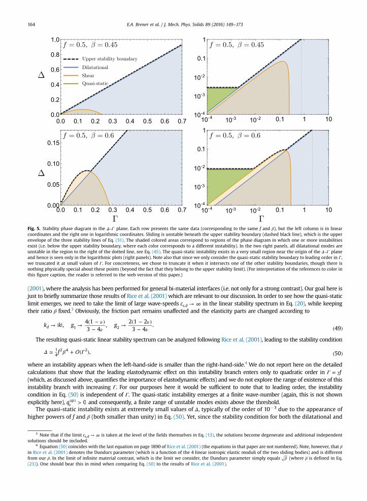
Fig. 5. Stability phase diagram in the Δ Γ– plane. Each row presents the same data (corresponding to the same f and β), but the left column is in linearcoordinates and the right one in logarithmic coordinates. Sliding is unstable beneath the upper stability boundary (dashed black line), which is the upperenvelope of the three stability lines of Eq. (51). The shaded colored areas correspond to regions of the phase diagram in which one or more instabilitiesexist (i.e. below the upper stability boundary, where each color corresponds to a different instability). In the two right panels, all dilatational modes areunstable in the region to the right of the dotted line, see Eq. (45). The quasi-static instability exists in a very small region near the origin of the Δ Γ– planeand hence is seen only in the logarithmic plots (right panels). Note also that since we only consider the quasi-static stability boundary to leading order in Γ,we truncated it at small values of Γ. For concreteness, we chose to truncate it when it intersects one of the other stability boundaries, though there isnothing physically special about these points (beyond the fact that they belong to the upper stability limit). (For interpretation of the references to color inthis figure caption, the reader is referred to the web version of this paper.)

E.A. Brener et al. / J. Mech. Phys. Solids 89 (2016) 149–173164

(2001), where the analysis has been performed for general bi-material interfaces (i.e. not only for a strong contrast). Our goal here isjust to briefly summarize those results of Rice et al. (2001) which are relevant to our discussion. In order to see how the quasi-staticlimit emerges, we need to take the limit of large wave-speeds → ∞cs d, in the linear stability spectrum in Eq. (20), while keepingtheir ratio β fixed.3 Obviously, the friction part remains unaffected and the elasticity parts are changed according to

νν

νν

→ | | → ( − )−

→ ( − )− ( )k k g g,

4 13 4

,2 1 2

3 4. 49d 1 2

The resulting quasi-static linear stability spectrum can be analyzed following Rice et al. (2001), leading to the stability condition

Δ β Γ≃ + ( ) ( )f , 5014

2 4 2

where an instability appears when the left-hand-side is smaller than the right-hand-side.4 We do not report here on the detailedcalculations that show that the leading elastodynamic effect on this instability branch enters only to quadratic order in Γ γ= f(which, as discussed above, quantifies the importance of elastodynamic effects) and we do not explore the range of existence of thisinstability branch with increasing Γ. For our purposes here it would be sufficient to note that to leading order, the instabilitycondition in Eq. (50) is independent of Γ. The quasi-static instability emerges at a finite wave-number (again, this is not shownexplicitly here), >( )q 0c

qs and consequently, a finite range of unstable modes exists above the threshold.The quasi-static instability exists at extremely small values of Δ, typically of the order of 10�3 due to the appearance of

higher powers of f and β (both smaller than unity) in Eq. (50). Yet, since the stability condition for both the dilatational and

3 Note that if the limit → ∞cs d, is taken at the level of the fields themselves in Eq. (13), the solutions become degenerate and additional independentsolutions should be included.

4 Equation (50) coincides with the last equation on page 1890 of Rice et al. (2001) (the equations in that paper are not numbered). Note, however, that βin Rice et al. (2001) denotes the Dundurs parameter (which is a function of the 4 linear isotropic elastic moduli of the two sliding bodies) and is differentfrom our β. In the limit of infinite material contrast, which is the limit we consider, the Dundurs parameter simply equals β (where β is defined in Eq.(23)). One should bear this in mind when comparing Eq. (50) to the results of Rice et al. (2001).

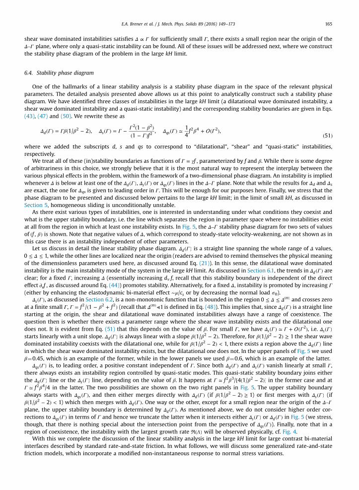
E.A. Brener et al. / J. Mech. Phys. Solids 89 (2016) 149–173 165

shear wave dominated instabilities satisfies Δ Γ∝ for sufficiently small Γ, there exists a small region near the origin of theΔ Γ– plane, where only a quasi-static instability can be found. All of these issues will be addressed next, where we constructthe stability phase diagram of the problem in the large kH limit.

6.4. Stability phase diagram

One of the hallmarks of a linear stability analysis is a stability phase diagram in the space of the relevant physicalparameters. The detailed analysis presented above allows us at this point to analytically construct such a stability phasediagram. We have identified three classes of instabilities in the large kH limit (a dilatational wave dominated instability, ashear wave dominated instability and a quasi-static instability) and the corresponding stability boundaries are given in Eqs.(43), (47) and (50). We rewrite these as

Δ Γ Γβ β Δ Γ Γ Γ βΓ

Δ Γ β Γ( ) = ( − ) ( ) = − ( − )( − )

( ) ≃ + ( )( )f

f1/ 2 ,1

1,

14

,51

d s qs2

2 2

22 4 2

where we added the subscripts d, s and qs to correspond to “dilatational”, “shear” and “quasi-static” instabilities,respectively.

We treat all of these (in)stability boundaries as functions of Γ γ= f , parameterized by f and β. While there is some degreeof arbitrariness in this choice, we strongly believe that it is the most natural way to represent the interplay between thevarious physical effects in the problem, within the framework of a two-dimensional phase diagram. An instability is impliedwhenever Δ is below at least one of the Δ Γ( )d , Δ Γ( )s or Δ Γ( )qs lines in the Δ Γ– plane. Note that while the results for Δd and Δs

are exact, the one for Δqs is given to leading order in Γ. This will be enough for our purposes here. Finally, we stress that thephase diagram to be presented and discussed below pertains to the large kH limit; in the limit of small kH, as discussed inSection 5, homogeneous sliding is unconditionally unstable.

As there exist various types of instabilities, one is interested in understanding under what conditions they coexist andwhat is the upper stability boundary, i.e. the line which separates the region in parameter space where no instabilities existat all from the region in which at least one instability exists. In Fig. 5, the Δ Γ– stability phase diagram for two sets of valuesof β( )f , is shown. Note that negative values of Δ, which correspond to steady-state velocity-weakening, are not shown as inthis case there is an instability independent of other parameters.

Let us discuss in detail the linear stability phase diagram. Δ Γ( )d is a straight line spanning the whole range of Δ values,Δ≤ ≤0 1, while the other lines are localized near the origin (readers are advised to remind themselves the physical meaning

of the dimensionless parameters used here, as discussed around Eq. (21)). In this sense, the dilatational wave dominatedinstability is the main instability mode of the system in the large kH limit. As discussed in Section 6.1, the trends in Δ Γ( )d areclear; for a fixed Γ, increasing Δ (essentially increasing dv f, recall that this stability boundary is independent of the directeffect ∂ fv , as discussed around Eq. (44)) promotes stability. Alternatively, for a fixed Δ, instability is promoted by increasing Γ

(either by enhancing the elastodynamic bi-material effect μ∼ c/ s or by decreasing the normal load s0).Δ Γ( )s , as discussed in Section 6.2, is a non-monotonic function that is bounded in the region Δ Δ≤ ≤ ( )0 m and crosses zero

at a finite small Γ, Γ β= ( − + )f f/ 12 2 2 (recall that Δ ⪡( ) 1m is defined in Eq. (48)). This implies that, since Δ Γ( )d is a straight linestarting at the origin, the shear and dilatational wave dominated instabilities always have a range of coexistence. Thequestion then is whether there exists a parameter range where the shear wave instability exists and the dilatational onedoes not. It is evident from Eq. (51) that this depends on the value of β. For small Γ, we have Δ Γ Γ Γ( ) ≃ + ( )s

2 , i.e. Δ Γ( )s

starts linearly with a unit slope. Δ Γ( )d is always linear with a slope β β( − )1/ 22 . Therefore, for β β( − ) ≥1/ 2 12 the shear wavedominated instability coexists with the dilatational one, while for β β( − ) <1/ 2 12 , there exists a region above the Δ Γ( )d linein which the shear wave dominated instability exists, but the dilatational one does not. In the upper panels of Fig. 5 we usedβ¼0.45, which is an example of the former, while in the lower panels we used β¼0.6, which is an example of the latter.

Δ Γ( )qs is, to leading order, a positive constant independent of Γ. Since both Δ Γ( )d and Δ Γ( )s vanish linearly at small Γ,there always exists an instability region controlled by quasi-static modes. This quasi-static stability boundary joins eitherthe Δ Γ( )d line or the Δ Γ( )s line, depending on the value of β. It happens at Γ β β≃ [ ( − )]f / 4 1/ 22 3 2 in the former case and atΓ β≃ f /42 4 in the latter. The two possibilities are shown on the two right panels in Fig. 5. The upper stability boundaryalways starts with Δ Γ( )qs , and then either merges directly with Δ Γ( )d (if β β( − ) ≥1/ 2 12 ) or first merges with Δ Γ( )s (ifβ β( − ) <1/ 2 12 ) which then merges with Δ Γ( )d . One way or the other, except for a small region near the origin of the Δ Γ–plane, the upper stability boundary is determined by Δ Γ( )d . As mentioned above, we do not consider higher order cor-rections to Δ Γ( )qs in terms of Γ and hence we truncate the latter when it intersects either Δ Γ( )s or Δ Γ( )d in Fig. 5 (we stress,though, that there is nothing special about the intersection point from the perspective of Δ Γ( )qs ). Finally, note that in aregion of coexistence, the instability with the largest growth rate R Λ( ) will be observed physically, cf. Fig. 4.

With this we complete the discussion of the linear stability analysis in the large kH limit for large contrast bi-materialinterfaces described by standard rate-and-state friction. In what follows, we will discuss some generalized rate-and-statefriction models, which incorporate a modified non-instantaneous response to normal stress variations.

E.A. Brener et al. / J. Mech. Phys. Solids 89 (2016) 149–173166

7. Generalized friction models: modified response to normal stress variations

Up to now we considered the standard rate-and-state friction model in which the frictional resistance does not exhibit a finitetime response to variations in the local normal stress. That is, the friction stress τ( )x t, was affected by the local interfacial normalstress σ( )x t, only through Eq. (11), and the response was instantaneous. Nevertheless, some experimental work (Linker and Diet-erich, 1992; Dieterich and Linker, 1992; Prakash and Clifton, 1992, 1993; Prakash, 1998; Richardson and Marone, 1999; Bureau et al.,2000) indicated that the frictional resistance may exhibit a finite time response to normal stress variations. To take this possibilityinto account we adopt here two experimentally-based modifications of the constitutive relation and incorporate them into ageneralized analysis. The goal is to understand the physical effects of the modified constitutive relations on the stability analysis.

The first modification we consider is due to Prakash and Clifton (1992, 1993), and Prakash (1998) and amounts to takingthe time scale T in Eq. (10) to be finite. A finite T means that when the interfacial normal stress σ( )x t, varies, the frictionstress τ( )x t, does not immediately follow it as in Eq. (11). T is commonly expressed as α=T D v/PC , where αPC is a di-mensionless and a positive parameter which measures T in units of the already existing time scale in the model, D v/ .Consequently, τ σ ϕ( )F v, , , in Eq. (6) takes the form

τ τ σ ϕα

τ σ ϕ = ( ) = − ( − ( ))( )

F vv

Df v, , , , .

52PC

The instantaneous response in Eq. (11) is recovered in the limit α → 0PC . For any α > 0PC , the response is gradual such thatthe larger αPC the slower the response. As the variation of the interfacial normal stress σ( )x t, with slip (the elastodynamic bi-material effect) is the major destabilizing effect in the analysis presented up to now and since α > 0PC delays the destabi-lizing effect on the friction stress τ( )x t, , we expect α > 0PC to promote stability. The finite-time response to normal stressvariations in Eq. (52) has been invoked by several authors in relation to the regularization of the Coulomb friction law, forexample in the context of the stability of steady frictional sliding (Ranjith and Rice, 2001), which was already mentionedabove, and dynamic rupture propagation (Cochard and Rice, 2000; Ben-Zion and Huang, 2002) along bi-material interfaces.

The second modification we consider is due to Linker and Dieterich (Linker and Dieterich, 1992; Dieterich and Linker,1992), who interpreted their experiments as suggesting that the state variable ϕ is directly affected by variations in thenormal stress. In particular, they proposed that τ σ ϕ( )G v, , , in Eq. (6) takes the form

ϕ τ σ ϕ ϕ α σσ

= ( ) = − − ∂ ( )ϕ

G vvD f

, , , 1 ,53

LD

where αLD is a positive dimensionless parameter. When α = 0LD , Eq. (9) is recovered with ( ) = −g x x1 (note that ′( ) = −g 1 1).To qualitatively understand the effect of α > 0LD on the frictional stability, we consider a fast variation in the normal stress(i.e. a large σ| |) such that the last term on the right-hand-side of Eq. (53) dominates the other two terms. In this case, we caneliminate the time derivative to obtain

δϕα δσσ

σ δ α δσ≃ −∂

⟹ ≃ −( )ϕ f

f ,54

LDLD

00

where we set σ σ= 0.The last result may appear somewhat counterintuitive. To better understand it, note that for α = 0PC (which is assumed

here to simplify things), σ δf0 contributes to the variation of the friction stress δτ as in Eq. (12). According to Eq. (54), whenthe normal stress reduces, σ < 0, we have σ δ >f 00 which means the latter makes a positive contribution to the friction stress(for α > 0LD ). This appears to suggest that the bi-material effect in this case is stabilizing. This is not quite the case, becausethe effect of δσ on δτ contains in fact also the last term on the right-hand-side of Eq. (12). Together, we obtain δτ α δσ≃ ( − )f LD

(recall that δσ δσ= −yy ), which shows that as long as α>f LD, a reduction in the normal stress still leads to a reduction in δτ ,i.e. it remains a destabilizing effect (later on we will see that this is not a strict stability condition). Yet the magnitude of thedestabilizing effect is reduced when α > 0LD (i.e. it is determined by α−f LD instead of f alone), which indicates that themodification in Eq. (53), with α > 0LD , promotes stability. Consequently, the simple considerations discussed here suggestthat replacing Eqs. (9) and (11) with Eqs. (52) and (53), for α α >, 0LD PC , will facilitate stability.

Next, we aim at rigorously studying the generalized model, which incorporates the modified response to normal stressvariations in Eqs. (52) and (53), in the large kH limit. For that aim, we first derive the linear stability spectrum for this case.Contrary to the analysis in Section 6, we should explicitly include now perturbations of the friction stressτ τ Λ( ) = + [ − ]τx t A t ikx, exp0 since τ( )x t, satisfies a dynamical equation of its own. The linear stability spectrum reads

⎜ ⎟⎛⎝⎜

⎞⎠⎟

⎛⎝

⎞⎠μ α Λ μ

μα Λ

Λ

σ Λ

ΛΛ+ − +

++

+∂ + =

( )

kDv

g i kf gik g

vD

vD

fvD

d f1 0,

55d PC

LDv v

01 2

2

0

0

0

0

which reduces to Eq. (20) for α α= = 0LD PC , | ′( )| =g 1 1 and →g G1,2 1,2. The non-dimensional spectrum takes the form

⎡⎣⎢

⎤⎦⎥( )γ β β α β γ α β Δ( − ) − ( ) − − ( ) + ( ) − ( − ) = ( )iqz z g z i qz ifg z q g z z iz iqz1 1 , 1 , , 0,

56PC LD2 2

1 2 2

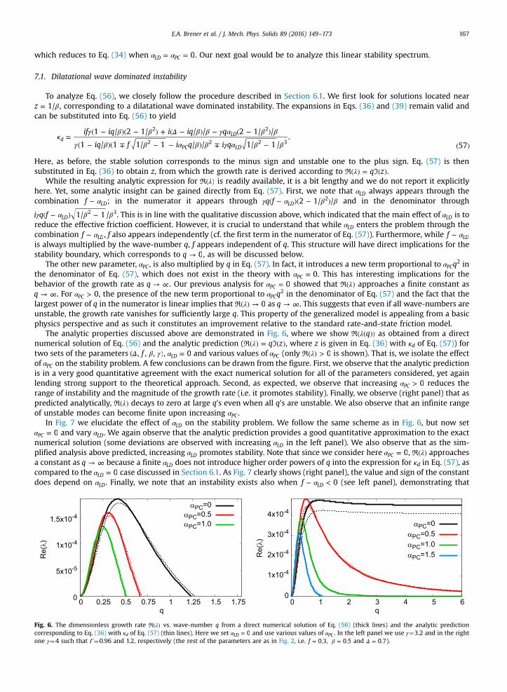
E.A. Brener et al. / J. Mech. Phys. Solids 89 (2016) 149–173 167

which reduces to Eq. (34) when α α= = 0LD PC . Our next goal would be to analyze this linear stability spectrum.

7.1. Dilatational wave dominated instability

To analyze Eq. (56), we closely follow the procedure described in Section 6.1. We first look for solutions located nearβ=z 1/ , corresponding to a dilatational wave dominated instability. The expansions in Eqs. (36) and (39) remain valid and

can be substituted into Eq. (56) to yield

κγ β β Δ β β γ α β β

γ β β α β β γ α β β≃

( − )( − ) + ( − ) − ( − )

( − )( ∓ − − ) ∓ − ( )

if iq i iq q

iq f i q i q

1 / 2 1/ / / 2 1/ /

1 / 1 1/ 1 / / 1/ 1 /.

57d

LD

PC LD

2 2

2 2 2 3

Here, as before, the stable solution corresponds to the minus sign and unstable one to the plus sign. Eq. (57) is thensubstituted in Eq. (36) to obtain z, from which the growth rate is derived according to R Iλ( ) = ( )q z .

While the resulting analytic expression for R λ( ) is readily available, it is a bit lengthy and we do not report it explicitlyhere. Yet, some analytic insight can be gained directly from Eq. (57). First, we note that αLD always appears through thecombination α−f LD; in the numerator it appears through γ α β β( − )( − )q f 2 1/ /LD

2 and in the denominator through

γ α β β( − ) −i q f 1/ 1 /LD2 3. This is in line with the qualitative discussion above, which indicated that the main effect of αLD is to

reduce the effective friction coefficient. However, it is crucial to understand that while αLD enters the problem through thecombination α−f LD, f also appears independently (cf. the first term in the numerator of Eq. (57)). Furthermore, while α−f LD

is always multiplied by the wave-number q, f appears independent of q. This structure will have direct implications for thestability boundary, which corresponds to →q 0, as will be discussed below.

The other new parameter, αPC , is also multiplied by q in Eq. (57). In fact, it introduces a new term proportional to α qPC2 in

the denominator of Eq. (57), which does not exist in the theory with α = 0PC . This has interesting implications for thebehavior of the growth rate as → ∞q . Our previous analysis for α = 0PC showed that R λ( ) approaches a finite constant as

→ ∞q . For α > 0PC , the presence of the new term proportional to α qPC2 in the denominator of Eq. (57) and the fact that the

largest power of q in the numerator is linear implies thatR λ( ) → 0 as → ∞q . This suggests that even if all wave-numbers areunstable, the growth rate vanishes for sufficiently large q. This property of the generalized model is appealing from a basicphysics perspective and as such it constitutes an improvement relative to the standard rate-and-state friction model.

The analytic properties discussed above are demonstrated in Fig. 6, where we show R λ( ( ))q as obtained from a directnumerical solution of Eq. (56) and the analytic prediction (R Iλ( ) = ( )q z , where z is given in Eq. (36) with κd of Eq. (57)) fortwo sets of the parameters Δ β γ( )f, , , , α = 0LD and various values of αPC (only R λ( ) > 0 is shown). That is, we isolate the effectof αPC on the stability problem. A few conclusions can be drawn from the figure. First, we observe that the analytic predictionis in a very good quantitative agreement with the exact numerical solution for all of the parameters considered, yet againlending strong support to the theoretical approach. Second, as expected, we observe that increasing α > 0PC reduces therange of instability and the magnitude of the growth rate (i.e. it promotes stability). Finally, we observe (right panel) that aspredicted analytically, R λ( ) decays to zero at large q's even when all q's are unstable. We also observe that an infinite rangeof unstable modes can become finite upon increasing αPC .

In Fig. 7 we elucidate the effect of αLD on the stability problem. We follow the same scheme as in Fig. 6, but now setα = 0PC and vary αLD. We again observe that the analytic prediction provides a good quantitative approximation to the exactnumerical solution (some deviations are observed with increasing αLD in the left panel). We also observe that as the sim-plified analysis above predicted, increasing αLD promotes stability. Note that since we consider here α = 0PC , R λ( ) approachesa constant as → ∞q because a finite αLD does not introduce higher order powers of q into the expression for κd in Eq. (57), ascompared to the α = 0LD case discussed in Section 6.1. As Fig. 7 clearly shows (right panel), the value and sign of the constantdoes depend on αLD. Finally, we note that an instability exists also when α− <f 0LD (see left panel), demonstrating that

0

5x10-5

1x10-4

1.5x10-4

0 0.25 0.5 0.75 1 1.25 1.5 1.75

Re(λ)

q

αPC=0αPC=0.5αPC=1.0

0

1x10-4

2x10-4

3x10-4

4x10-4

0 1 2 3 4 5 6

Re(λ)

q

αPC=0αPC=0.5αPC=1.0αPC=1.5

Fig. 6. The dimensionless growth rate R λ( ) vs. wave-number q from a direct numerical solution of Eq. (56) (thick lines) and the analytic predictioncorresponding to Eq. (36) with κd of Eq. (57) (thin lines). Here we set α = 0LD and use various values of αPC . In the left panel we use γ¼3.2 and in the rightone γ¼4 such that Γ¼0.96 and 1.2, respectively (the rest of the parameters are as in Fig. 2, i.e. β= =f 0.3, 0.5 and Δ = 0.7).

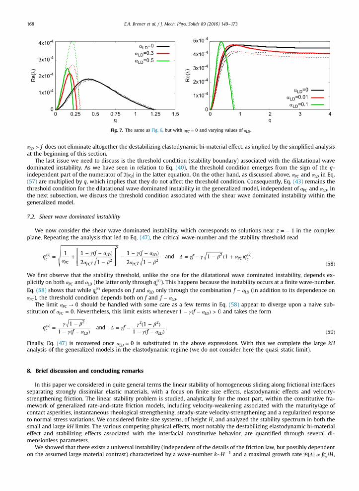
0

1x10-4

2x10-4

3x10-4

4x10-4

0 0.25 0.5 0.75 1 1.25 1.5

Re(λ)

q

αLD=0αLD=0.3αLD=0.5

0

1x10-4

2x10-4

3x10-4

4x10-4

5x10-4

0 1 2 3 4

Re(λ)

q

αLD=0αLD=0.01αLD=0.1

Fig. 7. The same as Fig. 6, but with α = 0PC and varying values of αLD.

E.A. Brener et al. / J. Mech. Phys. Solids 89 (2016) 149–173168

α > fLD does not eliminate altogether the destabilizing elastodynamic bi-material effect, as implied by the simplified analysisat the beginning of this section.

The last issue we need to discuss is the threshold condition (stability boundary) associated with the dilatational wavedominated instability. As we have seen in relation to Eq. (40), the threshold condition emerges from the sign of the q-independent part of the numerator of I κ[ ]d in the latter equation. On the other hand, as discussed above, αPC and αLD in Eq.(57) are multiplied by q, which implies that they do not affect the threshold condition. Consequently, Eq. (43) remains thethreshold condition for the dilatational wave dominated instability in the generalized model, independent of αPC and αLD. Inthe next subsection, we discuss the threshold condition associated with the shear wave dominated instability within thegeneralized model.

7.2. Shear wave dominated instability

We now consider the shear wave dominated instability, which corresponds to solutions near = −z 1 in the complexplane. Repeating the analysis that led to Eq. (47), the critical wave-number and the stability threshold read

⎡

⎣⎢⎢

⎤

⎦⎥⎥α

γ α

α γ β

γ α

α γ βΔ γ γ β α= +

− ( − )

−−

− ( − )

−= − − ( + )

( )

( ) ( )qf f

f q1 1

2 1

1

2 1and 1 1 .

58cs

PC

LD

PC

LD

PC

PC cs

2

2

22

We first observe that the stability threshold, unlike the one for the dilatational wave dominated instability, depends ex-plicitly on both αPC and αLD (the latter only through ( )qc

s ). This happens because the instability occurs at a finite wave-number.Eq. (58) shows that while ( )qc

s depends on f and αLD only through the combination α−f LD (in addition to its dependence onαPC), the threshold condition depends both on f and α−f LD.

The limit α → 0PC should be handled with some care as a few terms in Eq. (58) appear to diverge upon a naive sub-stitution of α = 0PC . Nevertheless, this limit exists whenever γ α− ( − ) >f1 0LD and takes the form

γ βγ α

Δ γ γ βγ α

=−

− ( − )= − ( − )

− ( − ) ( )( )q

ff

f1

1and

11

.59c

s

LD LD

2 2 2

Finally, Eq. (47) is recovered once α = 0LD is substituted in the above expressions. With this we complete the large kHanalysis of the generalized models in the elastodynamic regime (we do not consider here the quasi-static limit).

8. Brief discussion and concluding remarks

In this paper we considered in quite general terms the linear stability of homogeneous sliding along frictional interfacesseparating strongly dissimilar elastic materials, with a focus on finite size effects, elastodynamic effects and velocity-strengthening friction. The linear stability problem is studied, analytically for the most part, within the constitutive fra-mework of generalized rate-and-state friction models, including velocity-weakening associated with the maturity/age ofcontact asperities, instantaneous rheological strengthening, steady-state velocity-strengthening and a regularized responseto normal stress variations. We considered finite size systems, of height H, and analyzed the stability spectrum in both thesmall and large kH limits. The various competing physical effects, most notably the destabilizing elastodynamic bi-materialeffect and stabilizing effects associated with the interfacial constitutive behavior, are quantified through several di-mensionless parameters.

We showed that there exists a universal instability (independent of the details of the friction law, but possibly dependenton the assumed large material contrast) characterized by a wave-number k∼H�1 and a maximal growth rate R Λ[ ] ∝ fc H/s ,

E.A. Brener et al. / J. Mech. Phys. Solids 89 (2016) 149–173 169

mediated by waveguide-like modes. The role of boundary conditions for finite size systems has been also highlighted. Forlarge systems, → ∞H , we provided a comprehensive quantitative picture of the stability phase diagram. We showed that inaddition to the previously derived quasi-static instability modes (Rice et al., 2001), which exist at sufficiently small slidingvelocities, there exist also dilatational wave dominated instability modes propagating in the opposite direction to the slidingdirection and shear wave dominated instability modes propagating in the sliding direction. The former appear to be thedominant instability modes over a broad range of physical parameters. Our results allow us to determine, for every set ofphysical parameters relevant to a specific frictional system, which of the discussed instabilities features the largest growthrate. In a certain parameter range the instability is manifested through unstable modes at all wave-numbers, yet the fric-tional response is shown to be mathematically well-posed. The stabilizing roles played by a regularized response to normalstress variations are quantitatively accounted for.

All in all, our analysis shows that steady sliding along strong bi-material frictional interfaces is quite generically unstable,even in the presence of steady-state velocity-strengthening friction of a general form. The corresponding problem forsteady-state velocity-weakening friction is known to be generically unstable, but this instability is of different origincompared to the instabilities discussed in this paper. The discussed instabilities depend crucially on the destabilizing bi-material effect and consequently these generic instabilities are not expected to persist in frictional interfaces separatingidentical materials. Our results should be relevant to any frictional system exhibiting strong material contrast along thefrictional interface (and possibly also to finite contrast interfaces) and steady-state velocity-strengthening, for examplegeophysical systems such as mature earthquake faults (Ben-Zion, 2001, 2008) and engineering/tribological systems such asan elastic brake pad sliding on a rigid substrate (Behrendt et al., 2011).

The results of the linear stability analysis are possibly related to rupture dynamics along bi-material interfaces (Ben-Zion,2001, 2008). While the exact relations can be elucidated by following the instabilities into the nonlinear regime, mostprobably only numerically, one can speculate about these relations. For example, the dilatational wave dominated instability,which propagates in the direction opposite to the sliding motion and emerges at →k 0 (i.e. large wavelength), may cor-respond to crack-like (non-localized) super-shear rupture fronts propagating in the so-called “un-preferred direction” (i.e.opposite to the slip direction of the more compliant material, for any material contrast). Likewise, the shear wave dominatedinstability, which propagates in the direction of sliding motion and emerges at a finite k, may correspond to pulse-like(localized) shear rupture fronts propagating in the so-called “preferred direction” (i.e. the slip direction of the more com-pliant material, for any material contrast). These possible relations can be tested experimentally.

It would be interesting to quantify how the existence of a finite bi-material contrast affects the stability analysis pre-sented here for the large contrast limit, where the destabilizing elastodynamic bi-material effect is the largest. We hope toreport on this analysis in the near future. Furthermore, other theoretical issues should be considered; for example, as thedilatational and shear wave dominated instabilities propagate with high velocities in the lab frame of reference, issues ofabsolute vs. convective instabilities (Lifshitz and Pitaevskii, 1981; Huerre and Monkewitz, 1990) may become important.Moreover, in the presence of lateral boundaries (i.e. for realistic systems of finite size L in the x-direction) the so-calledglobal instability (Lifshitz and Pitaevskii, 1981; Huerre and Monkewitz, 1990) may be relevant due to the lateral boundaryconditions which induce a coupling between different linear propagating modes. Finally, the finite size L naturally implies amodification of some of the small wave-number instabilities discussed above.

Acknowledgements

E.B. acknowledges support of the James S. McDonnell Foundation, the Minerva Foundation with funding from the FederalGerman Ministry for Education, Research, the William Z. and Eda Bess Novick Young Scientist Fund and COST ActionMP1303. This research is made possible in part by the historic generosity of the Harold Perlman Family. R.S. acknowledgessupport by the DFG priority program 1713.

Appendix A. Derivation of Eq. (30)

We start by expanding first the basic functions appearing in Eq. (24) (see also Eq. (15)) as

ΛΛ

ΛΛ

δΛ Λ

( ) ≃ ± ( ) ≃ ±

( ) ≃ ± ( ) ≃ ± ( )( )

k kc

k kc

HkHc

Hk H c

, , , ,

coth , tanh tanh / ,A.1

dd

ss

dd

s s

0 0

0

where the 7 correspond to the stable/unstable branches, respectively. As will be seen right away, the distinction betweenthe two branches disappears in the final expression. Using these expansions, we obtain the following relevant combinations

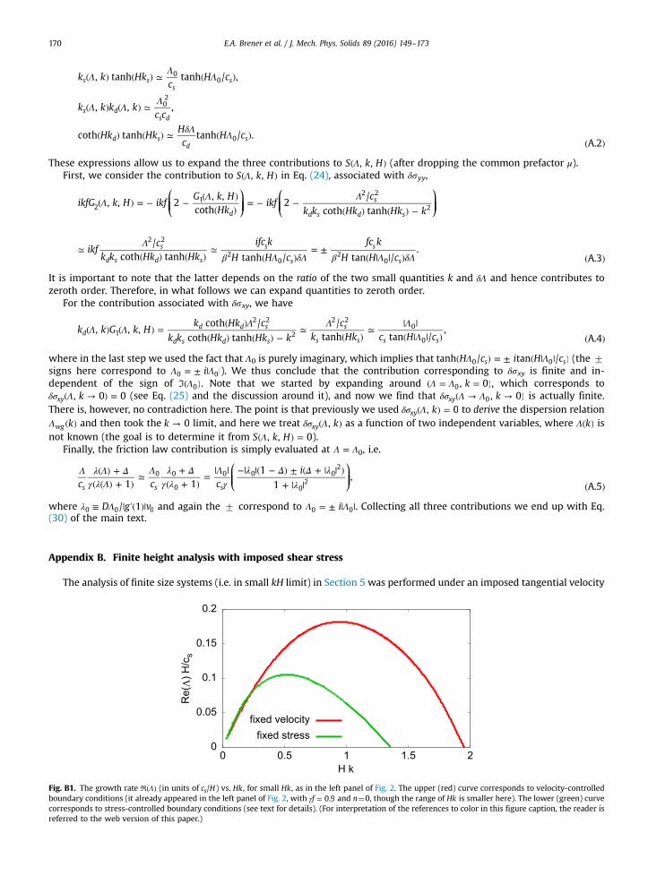
E.A. Brener et al. / J. Mech. Phys. Solids 89 (2016) 149–173170

ΛΛ

Λ

Λ ΛΛ

δΛ Λ

( ) ( ) ≃ ( )

( ) ( ) ≃

( ) ( ) ≃ ( )( )

k k Hkc

H c

k k k kc c

Hk HkHc

H c

, tanh tanh / ,

, , ,

coth tanh tanh / .A.2

s ss

s

s ds d

d sd

s

00

02

0

These expressions allow us to expand the three contributions to Λ( )S k H, , (after dropping the common prefactor μ).First, we consider the contribution to Λ( )S k H, , in Eq. (24), associated with δsyy,

⎛⎝⎜⎜

⎞⎠⎟⎟

⎛⎝⎜⎜

⎞⎠⎟⎟Λ

Λ Λ

Λβ Λ δΛ β Λ δΛ

( ) = − −( )

( )= − −

( ) ( ) −

≃( ) ( )

≃( )

= ±( | | ) ( )

ikfG k H ikfG k H

Hkikf

c

k k Hk Hk k

ikfc

k k Hk Hk

ifc k

H H c

fc k

H H c

, , 2, ,

coth2

/coth tanh

/coth tanh tanh / tan /

.A.3

d

s

d s d s

s

d s d s

s

s

s

s

21

2 2

2

2 2

20

20

It is important to note that the latter depends on the ratio of the two small quantities k and δΛ and hence contributes tozeroth order. Therefore, in what follows we can expand quantities to zeroth order.

For the contribution associated with δsxy, we have

Λ ΛΛ Λ Λ

Λ( ) ( ) =

( )( ) ( ) −

≃( )

≃| |( | | ) ( )

k k G k Hk Hk c

k k Hk Hk k

ck Hk c H c

, , ,coth /

coth tanh/

tanh tan /,

A.4d

d d s

d s d s

s

s s s s1

2 2

2

2 20

0

where in the last step we used the fact that Λ0 is purely imaginary, which implies that Λ Λ( ) = ± ( | | )H c i H ctanh / tan /s s0 0 (the 7signs here correspond to Λ Λ= ± | |i0 0 ). We thus conclude that the contribution corresponding to δsxy is finite and in-dependent of the sign of I Λ( )0 . Note that we started by expanding around Λ Λ( = = )k, 00 , which corresponds toδσ Λ( → ) =k, 0 0xy (see Eq. (25) and the discussion around it), and now we find that δσ Λ Λ( → → )k, 0xy 0 is actually finite.There is, however, no contradiction here. The point is that previously we used δσ Λ( ) =k, 0xy to derive the dispersion relationΛ ( )kwg and then took the →k 0 limit, and here we treat δσ Λ( )k,xy as a function of two independent variables, where Λ( )k isnot known (the goal is to determine it from Λ( ) =S k H, , 0).

Finally, the friction law contribution is simply evaluated at Λ Λ= 0, i.e.

⎛⎝⎜⎜

⎞⎠⎟⎟Λ λ Λ Δ

γ λ ΛΛ λ Δ

γ λΛ

γλ Δ Δ λ

λ( ) +

( ( ) + )≃

+( + )

=| | −| |( − ) ± ( + | | )

+ | | ( )c c ci

1 11

1,

A.5s s s

0 0

0

0 0 02

02

where λ Λ≡ | ′( )|D g v/ 10 0 0 and again the 7 correspond to Λ Λ= ± | |i0 0 . Collecting all three contributions we end up with Eq.(30) of the main text.

Appendix B. Finite height analysis with imposed shear stress

The analysis of finite size systems (i.e. in small kH limit) in Section 5 was performed under an imposed tangential velocity

0

0.05

0.1

0.15

0.2

0 0.5 1 1.5 2

Re(Λ

) H/c

s

H k

fixed velocityfixed stress

Fig. B1. The growth rate R Λ( ) (in units of c H/s ) vs. Hk, for small Hk, as in the left panel of Fig. 2. The upper (red) curve corresponds to velocity-controlledboundary conditions (it already appeared in the left panel of Fig. 2, with γ =f 0.9 and n¼0, though the range of Hk is smaller here). The lower (green) curvecorresponds to stress-controlled boundary conditions (see text for details). (For interpretation of the references to color in this figure caption, the reader isreferred to the web version of this paper.)

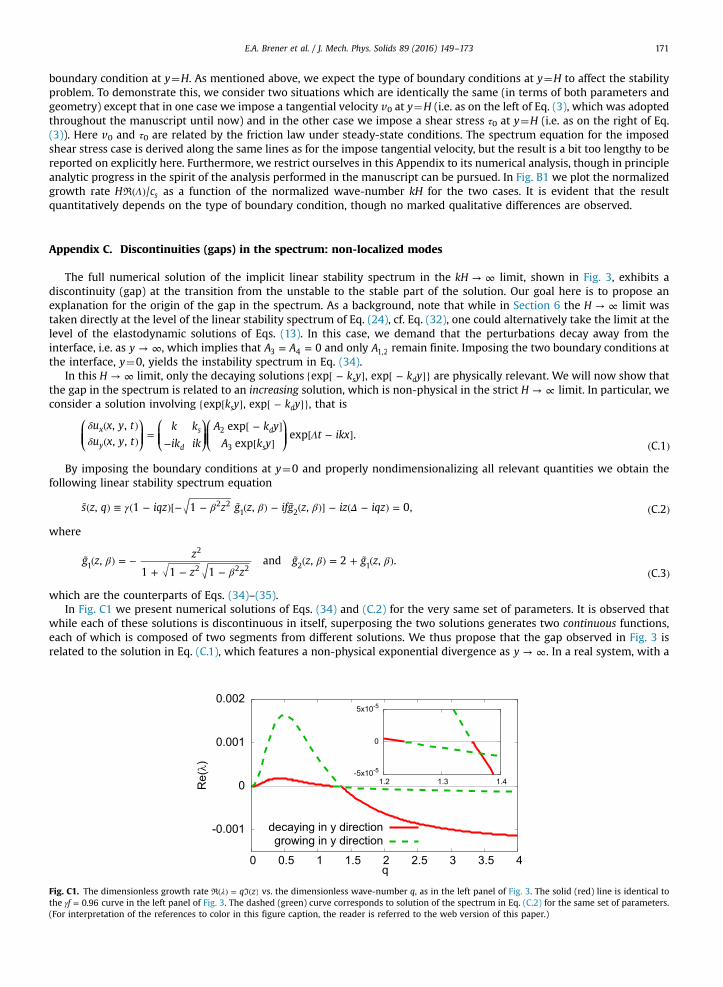
E.A. Brener et al. / J. Mech. Phys. Solids 89 (2016) 149–173 171

boundary condition at y¼H. As mentioned above, we expect the type of boundary conditions at y¼H to affect the stabilityproblem. To demonstrate this, we consider two situations which are identically the same (in terms of both parameters andgeometry) except that in one case we impose a tangential velocity v0 at y¼H (i.e. as on the left of Eq. (3), which was adoptedthroughout the manuscript until now) and in the other case we impose a shear stress τ0 at y¼H (i.e. as on the right of Eq.(3)). Here v0 and τ0 are related by the friction law under steady-state conditions. The spectrum equation for the imposedshear stress case is derived along the same lines as for the impose tangential velocity, but the result is a bit too lengthy to bereported on explicitly here. Furthermore, we restrict ourselves in this Appendix to its numerical analysis, though in principleanalytic progress in the spirit of the analysis performed in the manuscript can be pursued. In Fig. B1 we plot the normalizedgrowth rate R Λ( )H c/ s as a function of the normalized wave-number kH for the two cases. It is evident that the resultquantitatively depends on the type of boundary condition, though no marked qualitative differences are observed.

Appendix C. Discontinuities (gaps) in the spectrum: non-localized modes

The full numerical solution of the implicit linear stability spectrum in the → ∞kH limit, shown in Fig. 3, exhibits adiscontinuity (gap) at the transition from the unstable to the stable part of the solution. Our goal here is to propose anexplanation for the origin of the gap in the spectrum. As a background, note that while in Section 6 the → ∞H limit wastaken directly at the level of the linear stability spectrum of Eq. (24), cf. Eq. (32), one could alternatively take the limit at thelevel of the elastodynamic solutions of Eqs. (13). In this case, we demand that the perturbations decay away from theinterface, i.e. as → ∞y , which implies that = =A A 03 4 and only A1,2 remain finite. Imposing the two boundary conditions atthe interface, y¼0, yields the instability spectrum in Eq. (34).

In this → ∞H limit, only the decaying solutions { [ − ] [ − ]}k y k yexp , exps d are physically relevant. We will now show thatthe gap in the spectrum is related to an increasing solution, which is non-physical in the strict → ∞H limit. In particular, weconsider a solution involving { [ ] [ − ]}k y k yexp , exps d , that is

⎛⎝⎜⎜

⎞⎠⎟⎟

⎛⎝⎜⎜

⎞⎠⎟⎟⎛⎝⎜⎜

⎞⎠⎟⎟

δδ Λ

( )( ) =

−[ − ]

[ ][ − ]

( )

u x y tu x y t

k k

ik ik

A k y

A k yt ikx

, ,, ,

exp

expexp .

C.1

x

y

s

d

d

s

2

3

By imposing the boundary conditions at y¼0 and properly nondimensionalizing all relevant quantities we obtain thefollowing linear stability spectrum equation

γ β β β Δ˜( ) ≡ ( − )[− − ˜ ( ) − ˜ ( )] − ( − ) = ( )s z q iqz z g z ifg z iz iqz, 1 1 , , 0, C.22 2

1 2

where

ββ

β β˜ ( ) = −+ − −

˜ ( ) = + ˜ ( )( )

g zz

z zg z g z,

1 1 1and , 2 , .

C.31

2

2 2 2 2 1

which are the counterparts of Eqs. (34)–(35).In Fig. C1 we present numerical solutions of Eqs. (34) and (C.2) for the very same set of parameters. It is observed that

while each of these solutions is discontinuous in itself, superposing the two solutions generates two continuous functions,each of which is composed of two segments from different solutions. We thus propose that the gap observed in Fig. 3 isrelated to the solution in Eq. (C.1), which features a non-physical exponential divergence as → ∞y . In a real system, with a

-0.001

0

0.001

0.002

0 0.5 1 1.5 2 2.5 3 3.5 4

Re(λ)

q

decaying in y directiongrowing in y direction

-5x10-5

0

5x10-5

1.2 1.3 1.4

Fig. C1. The dimensionless growth rate R Iλ( ) = ( )q z vs. the dimensionless wave-number q, as in the left panel of Fig. 3. The solid (red) line is identical tothe γ =f 0.96 curve in the left panel of Fig. 3. The dashed (green) curve corresponds to solution of the spectrum in Eq. (C.2) for the same set of parameters.(For interpretation of the references to color in this figure caption, the reader is referred to the web version of this paper.)

E.A. Brener et al. / J. Mech. Phys. Solids 89 (2016) 149–173172

finite height H (however large), increasing solutions always exist and will naturally lead to the regularization of the dis-continuities that emerge in the strict → ∞H limit.

References

Achenbach, J., Epstein, H., 1967. Dynamic interaction of a layer and a half-space. J. Eng. Mech. Div. 93, 27–42.Adams, G.G., 1995. Self-excited oscillations of two elastic half-spaces sliding with a constant coefficient of friction. J. Appl. Mech. 62 (4), 867.Adams, G.G., 1998. Steady sliding of two elastic half-spaces with friction reduction due to interface stick-slip. J. Appl. Mech. 65 (2), 470.Adams, G.G., 2000. An intersonic slip pulse at a frictional interface between dissimilar materials. J. Appl. Mech. 68 (1), 81.Adda-Bedia, M., Ben Amar, M., 2003. Self-sustained slip pulses of finite size between dissimilar materials. J. Mech. Phys. Solids 51 (10), 1849–1861.Ampuero, J.-P., Ben-Zion, Y., 2008. Cracks, pulses and macroscopic asymmetry of dynamic rupture on a bimaterial interface with velocity-weakening

friction. Geophys. J. Int. 173 (2), 674–692.Andrews, D., Ben-Zion, Y., 1997. Wrinkle-like slip pulse on a fault between different materials. J. Geophys. Res. 102 (B1), 553.Baillet, L., Linck, V., D'Errico, S., Laulagnet, B., Berthier, Y., 2005. Finite element simulation of dynamic instabilities in frictional sliding contact. J. Tribol. 127

(3), 652.Bar Sinai, Y., Brener, E.A., Bouchbinder, E., 2012. Slow rupture of frictional interfaces. Geophys. Res. Lett. 39 (3), L03308.Bar-Sinai, Y., Spatschek, R., Brener, E.A., Bouchbinder, E., 2013. Instabilities at frictional interfaces: creep patches, nucleation, and rupture fronts. Phys. Rev. E

88 (6), 060403R.Bar-Sinai, Y., Spatschek, R., Brener, E.A., Bouchbinder, E., 2014. On the velocity-strengthening behavior of dry friction. J. Geophys. Res.: Solid Earth 119 (3),

1738–1748.Bar-Sinai, Y., Spatschek, R., Brener, E. A., Bouchbinder, E., 2015. Velocity-strengthening friction significantly affects interfacial dynamics, strength and

dissipation. Sci. Rep. 5, 7841. http://www.nature.com/articles/srep07841.Baumberger, T., Berthoud, P., 1999. Physical analysis of the state- and rate-dependent friction law. II. Dynamic friction. Phys. Rev. B 60 (6), 3928–3939.Baumberger, T., Caroli, C., 2006. Solid friction from stick-slip down to pinning and aging. Adv. Phys. 55 (3–4), 279–348.Behrendt, J., Weiss, C., Hoffmann, N.P., 2011. A numerical study on stick-slip motion of a brake pad in steady sliding. J. Sound Vib. 330 (4), 636–651.Ben-David, O., Rubinstein, S.M., Fineberg, J., 2010. Slip-stick and the evolution of frictional strength. Nature 463 (7277), 76–79.Ben-Zion, Y., 2001. Dynamic ruptures in recent models of earthquake faults. J. Mech. Phys. Solids 49 (9), 2209–2244.Ben-Zion, Y., 2008. Collective behavior of earthquakes and faults: continuum-discrete transitions, progressive evolutionary changes, and different dynamic

regimes. Rev. Geophys. 46 (4), RG4006.Ben-Zion, Y., Andrews, D., 1998. Properties and implications of dynamic rupture along a material interface. Bull. Seismol. Soc. Am. 88 (4), 1085–1094.Ben-Zion, Y., Huang, Y., 2002. Dynamic rupture on an interface between a compliant fault zone layer and a stiffer surrounding solid. J. Geophys. Res. 107

(B2), 2042.Berthoud, P., Baumberger, T., GSell, C., Hiver, J.-M., 1999. Physical analysis of the state- and rate-dependent friction law: static friction. Phys. Rev. B 59 (22),

14313–14327.Bureau, L., Baumberger, T., Caroli, C., 2000. Shear response of a frictional interface to a normal load modulation. Phys. Rev. E 62 (5), 6810–6820.Cochard, A., Rice, J.R., 2000. Fault rupture between dissimilar materials: Ill-posedness, regularization, and slip-pulse response. J. Geophys. Res. 105 (B11),

25891.Comninou, M., 1977a. Interface crack with friction in the contact zone. J. Appl. Mech. 44 (4), 780.Comninou, M., 1977b. The interface crack. J. Appl. Mech. 44 (4), 631.Comninou, M., Schmueser, D., 1979. The interface crack in a combined tension-compression and shear field. J.Appl. Mech. 46 (2), 345.Crupi, P., Bizzarri, A., 2013. The role of radiation damping in the modeling of repeated earthquake events. Ann. Geophys. 56 (1), R0111.Di Bartolomeo, M., Meziane, A., Massi, F., Baillet, L., Fregolent, A., 2010. Dynamic rupture at a frictional interface between dissimilar materials with as-

perities. Tribol. Int. 43 (9), 1620–1630.Dieterich, J.H., 1978. Time-dependent friction and the mechanics of stick-slip. Pure Appl. Geophys. 116 (4–5), 790–806.Dieterich, J.H., 1979. Modeling of rock Friction 1. experimental results and constitutive equations. J. Geophys. Res. 84 (B5), 2161–2168.Dieterich, J.H., 1992. Earthquake nucleation on faults with rate-and state-dependent strength. Tectonophysics 211 (1–4), 115–134.Dieterich, J.H., Kilgore, B.D., 1994. Direct observation of frictional contacts: new insights for state-dependent properties. Pure Appl. Geophys. 143 (1–3),

283–302.Dieterich, J.H., Linker, M.F., 1992. Fault stability under conditions of variable normal stress. Geophys. Res. Lett. 19 (16), 1691–1694.Gerde, E., Marder, M., 2001. Friction and fracture. Nature 413 (6853), 285–288.Harris, R.A., Day, S.M., 1997. Effects of a low-velocity zone on a dynamic rupture. Bull. Seismol. Soc. Am. 87 (5), 1267–1280.Hawthorne, J.C., Rubin, A.M., 2013. Tidal modulation and back-propagating fronts in slow slip events simulated with a velocity-weakening to velocity-

strengthening friction law. J. Geophys. Res.: Solid Earth 118 (3), 1216–1239.Heslot, F., Baumberger, T., Perrin, B., Caroli, B., Caroli, C., 1994. Creep, stick-slip, and dry-friction dynamics: experiments and a heuristic model. Phys. Rev. E

49 (6), 4973–4988.Huerre, P., Monkewitz, P.A., 1990. Local and global instability in spatially developing flows. Annu. Rev. Fluid Mech. 22, 473–537.Ibrahim, R.A., 1994a. Friction-induced vibration, chatter, squeal, and chaos. Part I: mechanics of contact and friction. Appl. Mech. Rev. 47 (7), 209–226.Ibrahim, R.A., 1994b. Friction-induced vibration, chatter, squeal, and chaos. Part II: dynamics and modeling. Appl. Mech. Rev. 47 (7), 227.Ikari, M.J., Marone, C.J., Saffer, D.M., Kopf, A.J., 2013. Slip weakening as a mechanism for slow earthquakes. Nat. Geosci. 6 (7), 468–472.Ikari, M.J., Saffer, D.M., Marone, C.J., 2009. Frictional and hydrologic properties of clay-rich fault gouge. J. Geophys. Res. 114 (B5), B05409.Kato, N., 2003. A possible model for large preseismic slip on a deeper extension of a seismic rupture plane. Earth Planet. Sci. Lett. 216 (1–2), 17–25.Lifshitz, E.M., Pitaevskii, L.P., 1981. Physical Kinetics. Pergamon, London.Linker, M.F., Dieterich, J.H., 1992. Effects of variable normal stress on rock friction: observations and constitutive equations. J. Geophys. Res. 97 (B4), 4923.Marone, C.J., 1998. Laboratory-derived friction laws and their application to seismic faulting. Annu. Rev. Earth Planet. Sci. 26 (1), 643–696.Marone, C.J., Scholz, C.H., 1988. The depth of seismic faulting and the upper transition from stable to unstable slip regimes. Geophys. Res. Lett. 15 (6),

621–624.Marone, C.J., Scholz, C.H., Bilham, R., 1991. On the mechanics of earthquake afterslip. J. Geophys. Res. 96 (B5), 8441.Martins, J., Guimaraes, J., Faria, L.O., 1995. Dynamic surface solutions in linear elasticity and viscoelasticity with frictional boundary conditions. J. Vib.

Acoust. 117 (4), 445–451.Martins, J., Simões, F.M.F., 1995. On some sources of instability/ill-posedness in elasticity problems with Coulomb's friction. In: Raous, M., Jean, M., Moreau,

J. (Eds.), Contact Mechanics. Springer, US, pp. 95–106.Meziane, A., D'Errico, S., Baillet, L., Laulagnet, B., 2007. Instabilities generated by friction in a pad-disc system during the braking process. Tribol. Int. 40 (7),

1127–1136.Nagata, K., Nakatani, M., Yoshida, S., 2008. Monitoring frictional strength with acoustic wave transmission. Geophys. Res. Lett. 35 (6), L06310.Nakatani, M., 2001. Conceptual and physical clarification of rate and state friction: frictional sliding as a thermally activated rheology. J. Geophys. Res. 106

(B7), 13347–13380.

E.A. Brener et al. / J. Mech. Phys. Solids 89 (2016) 149–173 173

Noda, H., Shimamoto, T., 2009. Constitutive properties of clayey fault gouge from the Hanaore fault zone, southwest Japan. J. Geophys. Res. 114 (B4), B04409.Perfettini, H., Ampuero, J.-P., 2008. Dynamics of a velocity strengthening fault region: implications for slow earthquakes and postseismic slip. J. Geophys.

Res. 113 (B9), B09411.Prakash, V., 1998. Frictional response of sliding interfaces subjected to time varying normal pressures. J. Tribol. 120 (1), 97.Prakash, V., Clifton, R.J., 1993. Time-resolved dynamic friction measurements in pressure-shear. In: Experimental Techniques in the Dynamics of De-

formable Solids, Applied Mechanics Division vol. 165 (AMD-vol. 165). American Society of Mechanical Engineers, New York, pp. 33–48.Prakash, V., Clifton, R. J., 1992. Pressure-shear plate impact measurement of dynamic friction for high speed machining applications. In: Proceedings of the

7th International Congress on Experimental Mechanics, pp. 8–11.Ranjith, K., 2009. Destabilization of long-wavelength Love and Stoneley waves in slow sliding. Int. J. Solids Struct. 46 (16), 3086–3092.Ranjith, K., 2014. Instabilities in dynamic anti-plane sliding of an elastic layer on a dissimilar elastic half-space. J. Elast. 115 (1), 47–59.Ranjith, K., Rice, J.R., 2001. Slip dynamics at an interface between dissimilar materials. J. Mech. Phys. Solids 49 (2), 341–361.Renardy, M., 1992. Ill-posedness at the boundary for elastic solids sliding under Coulomb friction. J. Elast. 27 (3), 281–287.Rice, J.R., 1993. Spatio-temporal complexity of slip on a fault. J. Geophys. Res. 98 (B6), 9885.Rice, J.R., Lapusta, N., Ranjith, K., 2001. Rate and state dependent friction and the stability of sliding between elastically deformable solids. J. Mech. Phys.

Solids 49 (9), 1865–1898.Rice, J.R., Ruina, A., 1983. Stability of steady frictional slipping. J. Appl. Mech. 50, 343.Richardson, E., Marone, C., 1999. Effects of normal stress vibrations on frictional healing. J. Geophys. Res. 104 (B12), 28859.Ruina, A., 1983. Slip instability and state variable friction laws. J. Geophys. Res. 88 (B12), 10359–10370.Scholz, C.H., 2002. The Mechanics of Earthquakes and Faulting. Cambridge University Press, Cambridge, UK.Shibazaki, B., Iio, Y., 2003. On the physical mechanism of silent slip events along the deeper part of the seismogenic zone. Geophys. Res. Lett. 30 (9), 1489.Simões, F.M.F., Martins, J., 1998. Instability and ill-posedness in some friction problems. Int. J. Eng. Sci. 36 (11), 1265–1293.Teufel, L.W., Logan, J.M., 1978. Effect of displacement rate on the real area of contact and temperatures generated during frictional sliding of Tennessee

sandstone. Pure Appl. Geophys. 116 (4–5), 840–865.Tonazzi, D., Massi, F., Culla, A., Baillet, L., Fregolent, A., Berthier, Y., 2013. Instability scenarios between elastic media under frictional contact. Mech. Syst.

Signal Process. 40 (2), 754–766.Weeks, J.D., 1993. Constitutive laws for high-velocity frictional sliding and their influence on stress drop during unstable slip. J. Geophys. Res. 98 (B10),

17637.Weertman, J., 1963. Dislocations moving uniformly on the interface between isotropic media of different elastic properties. J. Mech. Phys. Solids 11 (3),

197–204.Weertman, J., 1980. Unstable slippage across a fault that separates elastic media of different elastic constants. J. Geophys. Res. 85 (B3), 1455.Xia, K., Rosakis, A.J., Kanamori, H., 2004. Laboratory earthquakes: the sub-Rayleigh-to-supershear rupture transition. Science 303 (5665), 1859–1861.