dynamic behavior of measurement systems - … · 2009-09-01 · 3 dynamic behavior of measurement...

MAE 334 - INTRODUCTION TO COMPUTERS AND INSTRUMENTATION

MeasurementSystemBehaviorNotes.docx 1 of 12 9/11/2009 Scott H Woodward

3 Dynamic Behavior of Measurement Systems

Order of a Dynamic Measurement System

Every measurement system responds to inputs in a unique way. For

example, your ability to hear high frequency sounds will probably degrade

as you age and will never be as keen as most dogs hearing. Sound

pressure waves are a dynamic signal and the sensing of these pressure

waves by a flexible membrane (like your ear drum) can be mathematically

modeled and therefore simulated.

Our goal in this section is to apply our understanding of the physics

involved in sensing a signal and build a mathematical model that could be

used to describe the response of the measurement system to a dynamic

signal. In prior sections we described the response of a measurement

system to a static signal and built a mathematical model which described

that response. The process of characterizing that response is referred to

as a static calibration and the resulting mathematical model is called the

static calibration curve.

In the first lab you will perform both a static and dynamic calibration of a

temperature sensor and determine the corresponding static and dynamic

models which describe the sensor response. In the case of a signal that is

changing with time (dynamic) a sensor that can keep up, or is fast

enough, is needed to accurately detect the change. In the case of the

temperature sensors used in the first lab both the sensor and the

environment being sensed must be at the same temperature to make an

accurate measurement. If the sensor is initially at a different temperature

then some amount of time is required for the sensor and the environment

to become the same temperature. There has been a dynamic change in

the sensor temperature in response to a dynamic change in the input

temperature signal.

In this example we understand that heat must be transferred from the

environment to the sensor. The physics of that heat transfer might be

modeled based on our understanding of conduction, convection, radiation

or possibly some combination thereof. In general we could reason that

the temperature sensor performs some mathematical operation on the

input signal and outputs the result.

In fact most measurement systems can be modeled using a differential

equation that describes the relationship between the input signal and the

output signal. In the first lab you will find the linear equation that describes

the response to a static input (a static calibration) and the first order

differential equation that describes the conductive heat transfer to and

from the sensor (a dynamic calibration).



Figure 3.2 Measurement system operation on an input signal, F(t), provides the

output signal, y(t).

Measurement System Model

If the measurement system operation performed on the input signal, F(t),

in figure 3.2 is an nth-order linear differential equation then the output

signal, y(t), can be represented with the equation:

1

1 1 01( )

n n

n nn n

d y d y dya a a a y F t

dt dt dt (3.1)

where the coefficients, a0, a1, a2, …, an represent the physical system

parameters whose properties and values will depend on the

measurement system itself. The forcing function, F(t), can also be

generalized into an mth-order equation of the form:

1

1 1 01( )

m m

m mm m

d x d x dxF t b b b b x m n

dt dt dt

where b0, b1,…, bm also represent physical system parameters. The

nature of these equations should reflect the governing equations of the

pertinent fundamental physical laws of nature that are relevant to the

measurement system.

Zero-Order System

If all the derivatives in Equation 3.1 are zero then the most basic model of

a measurement system is obtained, the zero-order differential equation:

0 ( )a y F t

From this equation it is easy to see that any input, F(t), is instantly

reflected in the output y with only a factor, a0, modification. If the input is a

dynamically varying signal b0x then y = b0/a0x or y = Kx. The factor K is



often times referred to as the static sensitivity found during a static

calibration.

First-Order System

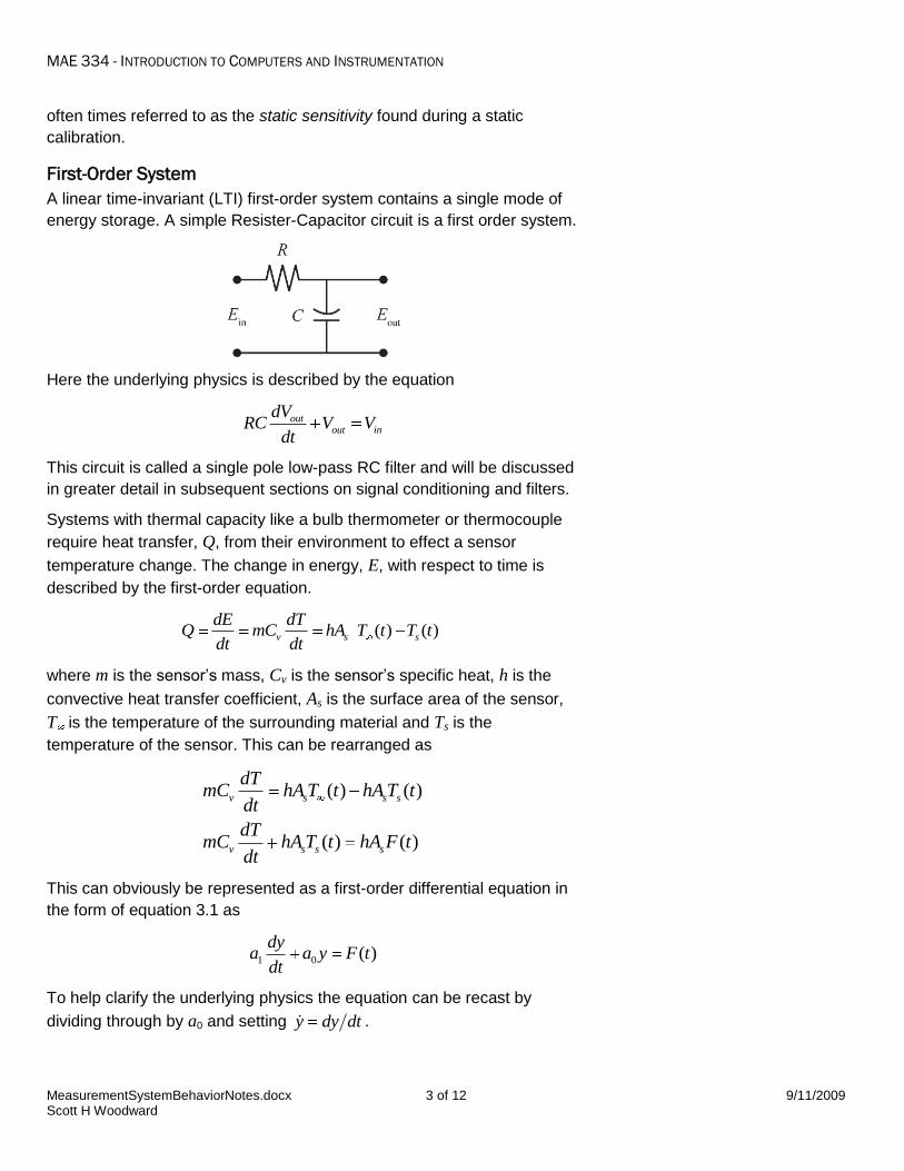
A linear time-invariant (LTI) first-order system contains a single mode of

energy storage. A simple Resister-Capacitor circuit is a first order system.

Here the underlying physics is described by the equation

outout in

dVRC V V

dt

This circuit is called a single pole low-pass RC filter and will be discussed

in greater detail in subsequent sections on signal conditioning and filters.

Systems with thermal capacity like a bulb thermometer or thermocouple

require heat transfer, Q, from their environment to effect a sensor

temperature change. The change in energy, E, with respect to time is

described by the first-order equation.

( ) ( )v s s

dE dTQ mC hA T t T t

dt dt

where m is the sensor’s mass, Cv is the sensor’s specific heat, h is the

convective heat transfer coefficient, As is the surface area of the sensor,

T is the temperature of the surrounding material and Ts is the

temperature of the sensor. This can be rearranged as

( ) ( )

( ) ( )

v s s s

v s s s

dTmC hA T t hA T t

dt

dTmC hA T t hA F t

dt

This can obviously be represented as a first-order differential equation in

the form of equation 3.1 as

1 0 ( )

dya a y F t

dt

To help clarify the underlying physics the equation can be recast by

dividing through by a0 and setting y dy dt .



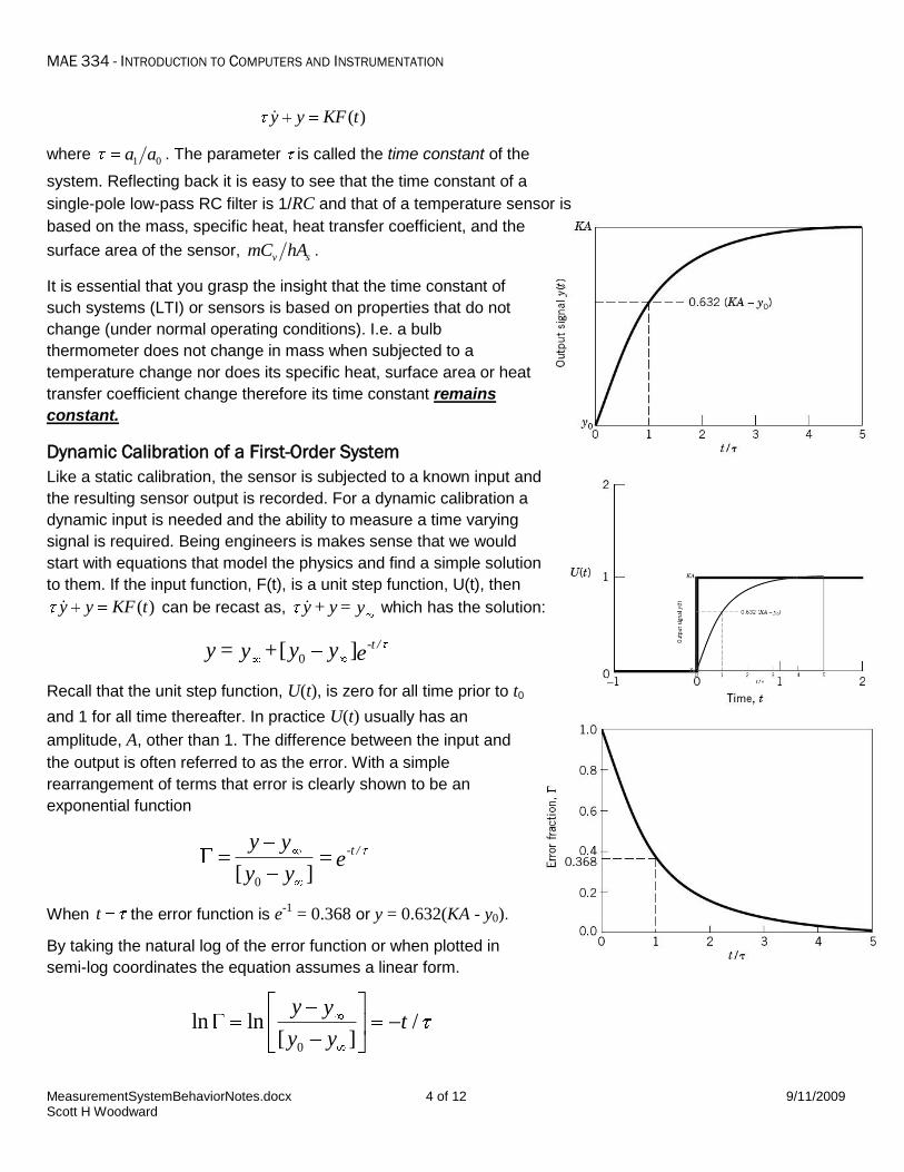
( )y y KF t

where 1 0a a . The parameter is called the time constant of the

system. Reflecting back it is easy to see that the time constant of a

single-pole low-pass RC filter is 1/RC and that of a temperature sensor is

based on the mass, specific heat, heat transfer coefficient, and the

surface area of the sensor, v smC hA .

It is essential that you grasp the insight that the time constant of

such systems (LTI) or sensors is based on properties that do not

change (under normal operating conditions). I.e. a bulb

thermometer does not change in mass when subjected to a

temperature change nor does its specific heat, surface area or heat

transfer coefficient change therefore its time constant remains

constant.

Dynamic Calibration of a First-Order System

Like a static calibration, the sensor is subjected to a known input and

the resulting sensor output is recorded. For a dynamic calibration a

dynamic input is needed and the ability to measure a time varying

signal is required. Being engineers is makes sense that we would

start with equations that model the physics and find a simple solution

to them. If the input function, F(t), is a unit step function, U(t), then

( )y y KF t can be recast as, y + y = y which has the solution:

0[ ] -t /y = + y yy e

Recall that the unit step function, U(t), is zero for all time prior to t0

and 1 for all time thereafter. In practice U(t) usually has an

amplitude, A, other than 1. The difference between the input and

the output is often referred to as the error. With a simple

rearrangement of terms that error is clearly shown to be an

exponential function

0[ ]

-t /y y

ey y

When t the error function is e-1

= 0.368 or y = 0.632(KA - y0).

By taking the natural log of the error function or when plotted in

semi-log coordinates the equation assumes a linear form.

0

ln ln /[ ]

y yt

y y



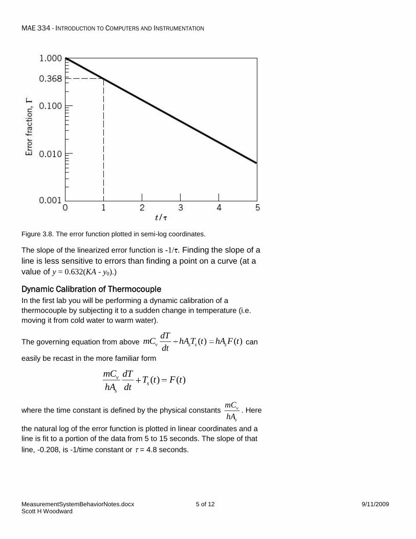
Figure 3.8. The error function plotted in semi-log coordinates.

The slope of the linearized error function is -1/ . Finding the slope of a

line is less sensitive to errors than finding a point on a curve (at a

value of y = 0.632(KA - y0).)

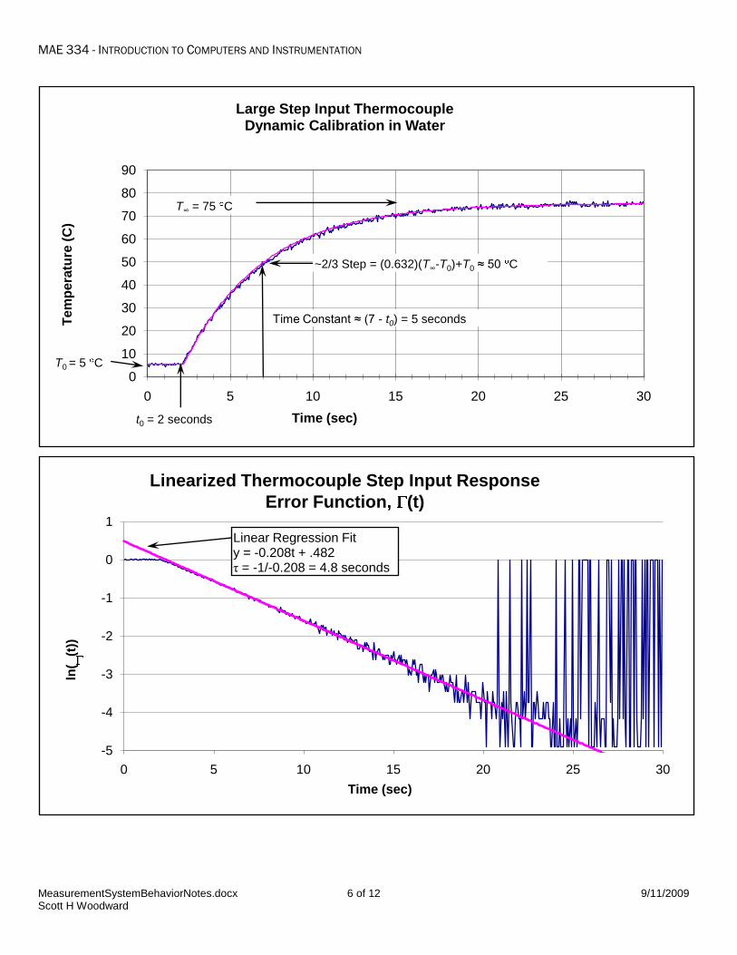
Dynamic Calibration of Thermocouple

In the first lab you will be performing a dynamic calibration of a

thermocouple by subjecting it to a sudden change in temperature (i.e.

moving it from cold water to warm water).

The governing equation from above ( ) ( )v s s s

dTmC hA T t hA F t

dt can

easily be recast in the more familiar form

( ) ( )vs

s

mC dTT t F t

hA dt

where the time constant is defined by the physical constants v

s

mC

hA. Here

the natural log of the error function is plotted in linear coordinates and a

line is fit to a portion of the data from 5 to 15 seconds. The slope of that

line, -0.208, is -1/time constant or = 4.8 seconds.



0

10

20

30

40

50

60

70

80

90

0 5 10 15 20 25 30

Te

mp

era

ture

(C

)

Time (sec)

Large Step Input Thermocouple Dynamic Calibration in Water

t0 = 2 seconds

T0 = 5 C

T∞ = 75 C

~2/3 Step = (0.632)(T∞-T0)+T0 ≈ 50 C

Time Constant ≈ (7 - t0) = 5 seconds

-5

-4

-3

-2

-1

0

1

0 5 10 15 20 25 30

ln(

(t))

Time (sec)

Linearized Thermocouple Step Input Response

Error Function, (t)

Linear Regression Fity = -0.208t + .482τ = -1/-0.208 = 4.8 seconds



An example data set using the same thermocouple containing

considerable noise and quantization error is plotted below. Of note is the

difficulty with which ~2/3 of the step response could be determined. In

contrast the time constant determined from the linearized error function is

relatively insensitive to the noise and quantization errors.

The line above is fit to only the first 2 seconds (~3 to 5 seconds) of the

linearized error function of the step input response and yields a = 4.8 s.

4

5

6

7

8

9

10

11

12

0 5 10 15 20 25 30

Te

mp

era

ture

(C

)

Time (sec)

Small Step Input Thermocouple Dynamic Calibration in Water

-3

-2.5

-2

-1.5

-1

-0.5

0

0.5

1

0 5 10 15 20 25 30

ln(

(t))

Time (sec)

Linearized Thermocouple Step Input Response

Error Function, (t)



Frequency Response of a First-Order System

The determination of the static sensitivity and time constant of a first-

order system transforms the black box “Measurement system operation”

in figure 3.2 into a known function. That implies that for any given output

which is correctly recorded the input that produced it could be

ascertained. This is possible because the differential equation describing

the physics of the measurement system is known and is solvable with

relative ease.

An intuitive description of the relationship between a system input and

output requires an understanding of the user, their intent as well as the

measurement system. Most users of thermometers are not interested in

dynamic temperature measurement. It is fair to say that few have the

training needed to relate the math to the physics and then apply this

knowledge to understand a dynamic phenomenon or solve a problem.

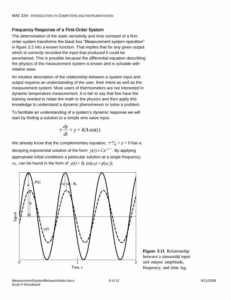
To facilitate an understanding of a system’s dynamic response we will

start by finding a solution to a simple sine wave input.

sin( )dy

+ y = KA tdt

We already know that the complementary equation, 0dydt + y = has a

decaying exponential solution of the form /( ) ty t Ce . By applying

appropriate initial conditions a particular solution at a single frequency,

1, can be found in the form of 1 1 1sin[ ( )]y(t)= B t+ .



For an input A1 sin( 1t) the output 1 1 1sin[ ( )]B t+ is produced. There

is an amplitude reduction from A1 to B1 and a delay in time, 1, reflected

in the phase shift of 1( ) .

The complete solution is

/( ) ( )sin[ ( )] ty t = B t+ +Ce

where

122( ) / 1 ( )B KA and 1( ) tan ( ) . This solution

depends only on the static sensitivity, K, and the time constant, . The

time constant is the only system characteristic that affects the frequency

response. This solution provides a relationship between the input and

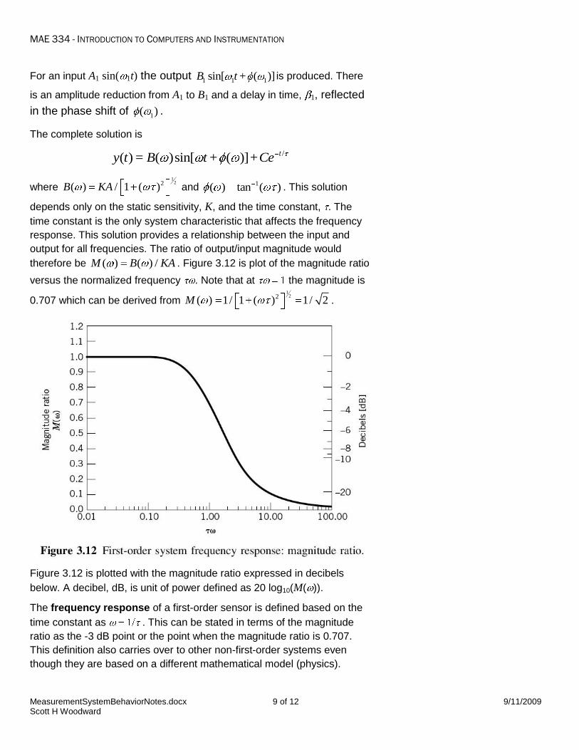
output for all frequencies. The ratio of output/input magnitude would

therefore be ( ( /) )M B KA . Figure 3.12 is plot of the magnitude ratio

versus the normalized frequency . Note that at the magnitude is

0.707 which can be derived from 1

22)( ) 1/ 1 ( 1/ 2M .

Figure 3.12 is plotted with the magnitude ratio expressed in decibels

below. A decibel, dB, is unit of power defined as 20 log10(M( )).

The frequency response of a first-order sensor is defined based on the

time constant as . This can be stated in terms of the magnitude

ratio as the -3 dB point or the point when the magnitude ratio is 0.707.

This definition also carries over to other non-first-order systems even

though they are based on a different mathematical model (physics).



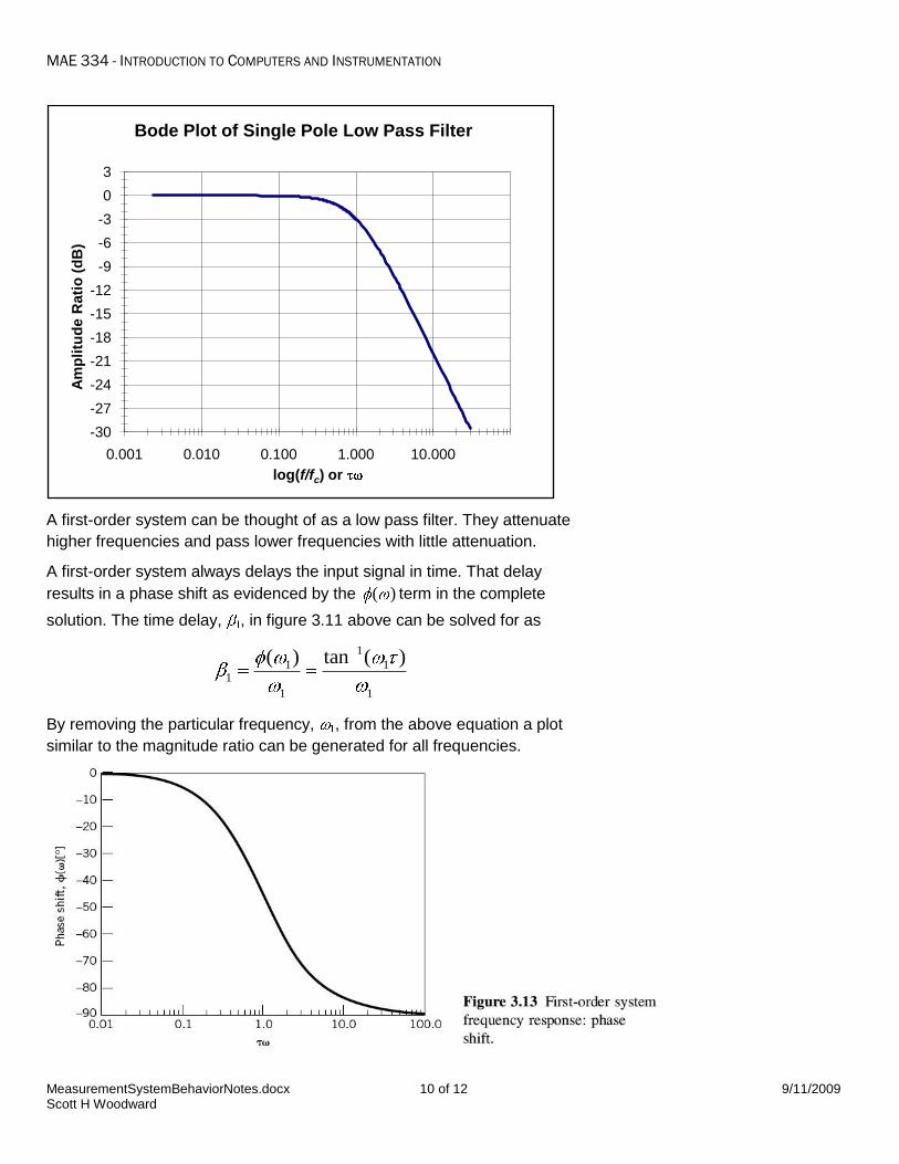
A first-order system can be thought of as a low pass filter. They attenuate

higher frequencies and pass lower frequencies with little attenuation.

A first-order system always delays the input signal in time. That delay

results in a phase shift as evidenced by the ( ) term in the complete

solution. The time delay, , in figure 3.11 above can be solved for as

11

1

1

1

1

t( ) an ( )

By removing the particular frequency, , from the above equation a plot

similar to the magnitude ratio can be generated for all frequencies.

-30

-27

-24

-21

-18

-15

-12

-9

-6

-3

0

3

0.001 0.010 0.100 1.000 10.000

Am

pli

tud

e R

ati

o (

dB

)

log(f/fc) or

Bode Plot of Single Pole Low Pass Filter



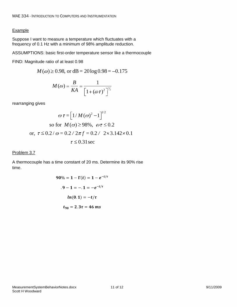
Example

Suppose I want to measure a temperature which fluctuates with a frequency of 0.1 Hz with a minimum of 98% amplitude reduction.

ASSUMPTIONS: basic first-order temperature sensor like a thermocouple

FIND: Magnitude ratio of at least 0.98

( 0.98, or dB 20log 0.98 0.175)M = =

122

1( )

1 ( )

BM

KA

rearranging gives

1/221/ ( ) 1

so for ( 98%, 0.2

or, 0.2 / 0.2 2 0.2 2 3.142 0

)

.1

0.31sec

= M

M

= / f = /

Problem 3.7

A thermocouple has a time constant of 20 ms. Determine its 90% rise

time.



Example 3.3

Suppose a bulb thermometer originally

indicating 20ºC is suddenly exposed to

a fluid temperature of 37 ºC. Develop

a simple model to simulate the

thermometer output response.

KNOWN:

T0 = 20ºC

T∞ = 37ºC

F(t) = [T∞ - T0]U(t)

ASSUMPTIONS:

Normal first-order response

FIND: T(t)

SOLUTION:

The rate at which energy is exchanged

between the sensor and the environment through convection, , must be

balanced by the storage of energy within the thermometer, dE/dt.

For a constant mass temperature sensor,

This can be written in the form

dividing by hAs

Therefore:

,

The thermometer response is therefore:

[ºC]

dynamic behavior of measurement systems - … · 2009-09-01 · 3 dynamic behavior of measurement...

Documents