duration models: parametric models - loginpsfaculty.ucdavis.edu/bsjjones/slide3_parm.pdf ·...

Bradford S. Jones, UC-Davis, Dept. of Political Science

Duration Models: Parametric Models

Brad Jones1

1Department of Political ScienceUniversity of California, Davis

January 28, 2011

Jones POL 290G

Bradford S. Jones, UC-Davis, Dept. of Political Science Parametric Survival Models

Parametric Survival Models

Jones POL 290G


Parametric Models

I Some Motivation for Parametrics

I Consider the hazard rate:

dh(t)

dt> 0,

Hazard increasing wrt time.

dh(t)

dt< 0,

Hazard decreasing wrt time.

dh(t)

dt= 0,

Hazard “flat” wrt time.

Jones POL 290G


Parametric Models

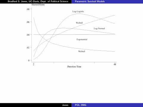
I Parametric models give structure (shape) to the hazardfunction.

I N.B.: the structure is a function of the c.d.f., not necessarilyof the “real world.”

I . . . though some c.d.f.s do a good job of approximating somefailure-time processes.

I Any c.d.f. with positive support on the real number line willwork.

I Lots of choices: exponential, Weibull, gamma, Gompertz,log-normal, log-logistic . . . etc.

Jones POL 290G


Jones POL 290G


Parametric Models

I For parametrics, we work with standard likelihood methods.

I Specify a distribution function and write out the log-likelihoodfor the data.

I The question is, which distribution function?

I In all software programs/computing environments, youre givena menu.

I Stata:streg, R:survreg, eha

Jones POL 290G


Parametric Models

I “Advantages” of parametric models?

I If S(t) is known to follow, or closely approximate a knowndistribution, then estimates will be consistent the thetheoretical survivor function.

I Unlike K-M or Cox (discussed later), the hazard may be usedfor forecasting (under KM or Cox, the hazard is only definedup until the last observed failure).

I Will return smooth functions of h(t) or S(t).

Jones POL 290G


Parametric Models

I As noted, there are a wide variety of choices.

I I sometimes refer to these choices as “plug and play”estimators.

I Why? Consider the survivor function:

S(t) = Pr(T > t) =

∫ ∞t

f (u)d(u) = 1−∫ t

0f (u)d(u) = 1−F (t)

(1)

I If we know this function follows some distribution, then wewrite a likelihood function in terms of this distribution . . .

I If it follows a different distribution, just replace the previouslikelihood with another pdf.

Jones POL 290G


Parametric Models

I Most texts, including ours, typically begin with theexponential distribution.

I The reason is easy: it’s an easy distribution to work with andvisualize.

I It also may be unrealistic in many settings.

I The basic feature: the hazard rate is flat wrt time.

I That is:h(t) = λ (2)

Jones POL 290G


Parametric Models

I Recall from the first week:

S(t) = exp{−H(t)} (3)

where

H(t) =

∫ t

0h(u)du

I Substituting λ into (3) ,

S(t) = exp{−∫ t

0λdu}

and soS(t) = exp(−λt)

I This is the survivor function for the exponential distribution.

Jones POL 290G


Parametric Models

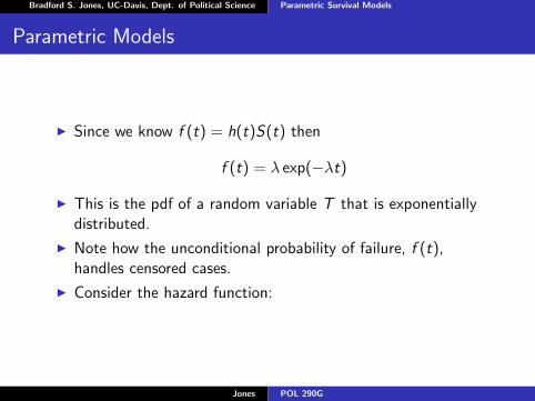
I Since we know f (t) = h(t)S(t) then

f (t) = λ exp(−λt)

I This is the pdf of a random variable T that is exponentiallydistributed.

I Note how the unconditional probability of failure, f (t),handles censored cases.

I Consider the hazard function:

Jones POL 290G


Jones POL 290G


Parametric Models

I What is λ?

I Or put differently, where are the predictor variables?

I Typically λ will be parameterized in terms of regressioncoefficients and covariates, X .

I A model:h(t) = λ = exp(β0 + β1T )

I Suppose T is a treatment indicator and we’re interested in thehazard of failure for the treated and untreated.

Jones POL 290G


Parametric Models

I Two hazards:

h(tT=1) = exp(β0 + β1)

h(tT=0) = exp(β0)

I If we plotted the hazards, we would have two parallel linesseparated by exp(β1).

I Or analogously, if we want to compare hazards:

h(tT=1)

h(tT=0)=

exp(β0 + β1)

exp(β0)

item¡4-¿ This expression must simplify to exp(β1).

Jones POL 290G


Parametric Models

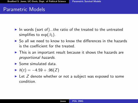
I In words (sort of)...the ratio of the treated to the untreatedsimplifies to exp(β1).

I So all we need to know to know the differences in the hazardsis the coefficient for the treated.

I This is an important result because it shows the hazards areproportional hazards.

I Some simulated data.

I h(t) = −4.59 + .96(Z )

I Let Z denote whether or not a subject was exposed to somecondition.

Jones POL 290G


Parametric Models

I Since β1 is positive, this implies exposure increases the risk.

I The hazard is higher for the exposed than for the unexposed.

I Treatment estimate is .96 implies difference in hazard isexp(.96) ≈ 2.6

I Risk for exposed is about 2.6 times greater than for theunexposed.

I Consider the hazards:

Jones POL 290G


Jones POL 290G


Parametric Models

I PH property is important to understand.

I By way of analogy, think about what odds ratios are in alogit-type setting or recall the ordered logit model: the OR areinvariant to the scale scores.

I The proportional difference in hazards is invariant to time.

I So under the exponential we are making two assumptions:1. The hazards are flat wrt time.2. The difference in hazards across levels of a covariate is afixed proportion.

I Which is the stronger assumption?

Jones POL 290G


Parametric Models

I Note that even with the PH assumption, we are not saying (ingeneral) the hazards are invariant to time (though in theexponential case, we are).

I The hazards may change but the proportional differencebetween (say) two groups, does not change.

I That’s the basic result of proportionality.

I Suppose it does not hold. Then what?

I Consider another model that relaxes the assumption of flathazards (but not the PH assumption).

Jones POL 290G


Parametric Models: Weibull

I A more flexible distribution function is given by the Weibull.

I Named for Waloddi Weibull, who derived it (1939, 1951)

I Why more general than the exponential?

I It is a two-parameter distribution:

h(t) = λptp−1 (4)

where λ is a positive scale parameter and p is a shapeparameter.

I Note:p > 1, the hazard rate is monotonically increasing with time.p < 1, the hazard rate is monotonically decreasing with time.p = 1, the hazard is flat.

Jones POL 290G



I Thus if p = 1 then

h(t) = λ1t1−1 = λ. (5)

I Thus demonstrating that the exponential model is nestedwithin the Weibull.

I For this reason (and for many other reasons), the Weibull isthe most commonly applied parametric model in survivalanalysis.

I As with the exponential, the scale parameter λ is usuallyexpressed in terms of covariates, exp(βkxi ).

I Hazard functions plotted for different p:

Jones POL 290G


Jones POL 290G



I Using the connection between S(t) and the cumulative hazard(see eq. [3]), the Weibull survivor function is given by

S(t) = exp{−∫ t

0λpup−1du} = exp(−λtp).

I And since the pdf is h(t)S(t), the density for a randomvariable T distributed as a Weibull is

f (t) = λptp−1 exp(−λtp).

I Suppose we estimate a Weibull hazard using the data frombefore.

Jones POL 290G


Jones POL 290G



I Note:h(tE )

h(tNE )=

exp(β0 + β1)ptp−1

exp(β0)ptp−1= exp(β1)

I In other words, the Weibull model is a proportional hazardsmodel.

I So unlike the exponential, the hazards can change wrt timebut like the exponential, the ratio of the hazards is a constant.

I They are offset by a proportionality factor of exp(β).

Jones POL 290G



I The Weibull (and therefore) the exponential are interestingmodels.

I They are both proportional hazards models as well asaccelerated failure time models.

I In other words, one can estimate the model in terms of thehazards or in terms of the survival times and reproduceequivalent results from different parameterizations.

I Under the PH model, the covariates are a multiplicative effectwith respect to the baseline hazard function (see previousslide).

I Under the AFT, the covariates are multiplicative wrt thesurvival time.

Jones POL 290G



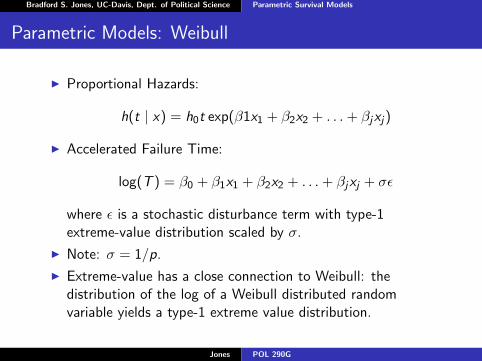
I Proportional Hazards:

h(t | x) = h0t exp(β1x1 + β2x2 + . . .+ βjxj)

I Accelerated Failure Time:

log(T ) = β0 + β1x1 + β2x2 + . . .+ βjxj + σε

where ε is a stochastic disturbance term with type-1extreme-value distribution scaled by σ.

I Note: σ = 1/p.

I Extreme-value has a close connection to Weibull: thedistribution of the log of a Weibull distributed randomvariable yields a type-1 extreme value distribution.

Jones POL 290G



I In the AFT formulation, the coefficients are sometimesreferred to as “acceleration” factors.

I They give information about how the survival times aredifferentially accelerated for different levels of a covariate.

I Suppose we estimate a treatment effect for two groups: Dand H.

I Imagine the estimated treatment effect yields a coefficient of“7.”

I That is, group H is estimated to survive 7 times longer thangroup D.

I SD(t) = SH(7t)

I If D are dogs and H are humans, the acceleration factorsuggests human lifespans are “stretched out” 7 times longerthan dogs. (Example from K and K, p. 266.)

Jones POL 290G



I Important to be aware of what your software is doing!

I The PH coefficients inform us about the hazard (i.e. risk).

I The AFT coefficients inform us about survival.

I Therefore, the coefficients will be signed differently.

Jones POL 290G



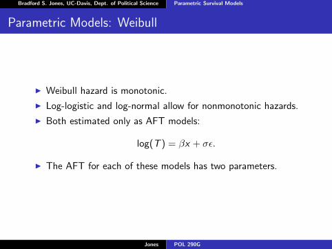
I Weibull hazard is monotonic.

I Log-logistic and log-normal allow for nonmonotonic hazards.

I Both estimated only as AFT models:

log(T ) = βx + σε.

I The AFT for each of these models has two parameters.

Jones POL 290G


Parametric Models: Log-Logistic

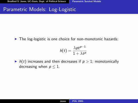
I The log-logistic is one choice for non-monotonic hazards:

h(t) =λptp−1

1 + λtp

I h(t) increases and then decreases if p > 1; monotonicallydecreasing when p ≤ 1.

Jones POL 290G


Jones POL 290G



I Again, λ gives information on the covariates (i.e. here iswhere the regression coefficients are.

I While the log-logistic is not a PH model, it is a proportionalodds model.

I Recall what this is from your previous course on MLE.

I Survivor function:

S(t) =1

1 + λtp=

λtp

1 + λtp

I Substitute exp(β) in for λ and you can see the connectionback to the logistic cdf.

Jones POL 290G



I The odds of failure:

1− S(t)

S(t)=

λtp

1+λtp

11+λtp

= λtp

I In terms of parameters, exponentiating β will give theacceleration factor.

I Interpretation is really quite similar to a logit model (but it isnot exactly the same!).

I Other models?

Jones POL 290G


Parametric Models: Estimation

I Previous can be estimated through MLE

I Imagine n observations upon which t1, t2, . . . tn duration timesare measured.

I Assume conditional independence of ti (may be herculeanassumption; more later)

I Specify a PDF (or CDF); if f (t) is derived, S(t) easily follows

I Write out likelihood function and maximize (standardalgorithm is Newton-Raphson)

Jones POL 290G


Parametric Models: Estimation

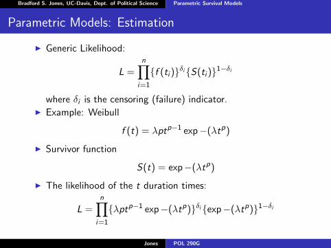
I Generic Likelihood:

L =n∏

i=1

{f (ti )}δi{S(ti )}1−δi

where δi is the censoring (failure) indicator.I Example: Weibull

f (t) = λptp−1 exp−(λtp)

I Survivor function

S(t) = exp−(λtp)

I The likelihood of the t duration times:

L =n∏

i=1

{λptp−1 exp−(λtp)}δi{exp−(λtp)}1−δi

Jones POL 290G


Getting Our Hands Dirty

I The only way to learn is to do.

I Useful to consider estimation and interpretation of someparametric models.

I Examples are based on cabinet duration data and most of thecode is in Stata.

I Stata do file is accessible on SmartSite and website.

Jones POL 290G


Exponential

I Cabinet duration as a function of post-election negotiationsindicator and formation attempts.

Table: Estimation results : PH Exponential

I

Variable Coefficient (Std. Err.)format 0.146 (0.039)postelec -1.036 (0.124)Intercept -2.762 (0.106)

Jones POL 290G


Exponential

I Coefficients are in PH scale so a positively signed coefficientimplies the hazard is increasing as a function of x .

I Post-election negotiations lowers the hazard; increasednumber of formation attempts increase the hazard.

I Graphical display of two covariate profiles.

Jones POL 290G


Jones POL 290G


Exponential

I Turn attention to the Stata examples (we will do this inclass).

I Consider the AFT model.

I Recall the AFT model:

log(T ) = βkxi + σε

I If ε is type-1 extreme value (aka Gumbel) then the Weibull isobtained. If σ = p = 1 then the exponential is obtained.

I The coefficients are multiples of the survivor function.

Jones POL 290G


Exponential

Table: Estimation results : AFT Exponential

Variable Coefficient (Std. Err.)format -0.146 (0.039)postelec 1.036 (0.124)Intercept 2.762 (0.106)

Jones POL 290G


Exponential

I Contrast the PH and AFT models.

I Under the exponential, the signs shift but the coefficients areunchanged in value.

I Sign shift makes sense: AFT formulation tells us aboutsurvivorship.

I AFT Hazard: −ho(t) exp−(xβ) = exp−(β0 + xβk)

I Solving for t: t = [− log(S(t)]× exp(β0 + β1 × postelec)

I If t = .5, we solve for the median survival time.

I Turn back to the Stata examples.

Jones POL 290G


Exponential

I From the application, note the equivalency of the two models.

I Note also that the ratio of two survival times for two covariateprofiles (i.e. X = 1 vs. X = 0) will be constant andproportional wrt S(t).

I Hence either parameterization exhibits proportionality.

I Weibull example.

Jones POL 290G


Weibull

I Under the exponential the hazard is flat..

I Under the Weibull:h(t) = λptp−1 (6)

λ is positive scale parameter; p is the shape parameter.

I p > 1, the hazard rate is monotonically increasing with time.

I p < 1, the hazard rate is monotonically decreasing with time.

I p = 1, the hazard is flat, i.e. exponential.

I Note that λ corresponds to covariates: exp(βkxi )

Jones POL 290G


Weibull hazards

I Consider application again.

Table: Estimation results : PH Weibull

I

Variable Coefficient (Std. Err.)

Equation 1 : t

format 0.156 (0.039)postelec -1.109 (0.129)Intercept -3.094 (0.199)

Equation 2 : ln p

Intercept 0.106 (0.050)

Jones POL 290G


Weibull

I Coefficients are interpreted as before though now we have anadditional parameter.

I p > 1 implying rising hazards for this model.

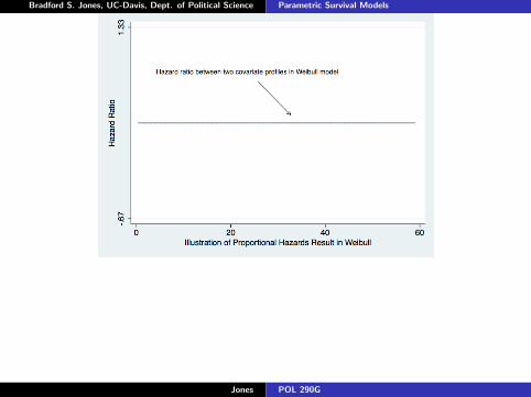
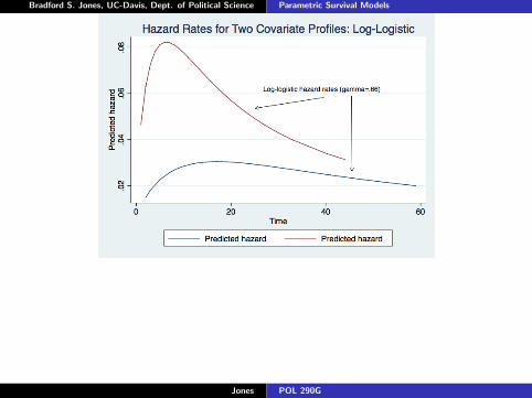
I Consider the hazard rates for two covariate profiles.

Jones POL 290G


Jones POL 290G


Weibull

I Observations?

I Note the shape is governed by p . . .

I But the difference in the two hazards are proportional.

I Looks may be deceiving; perhaps you think the lines shownonproportionality.

I Back to the application.

Jones POL 290G


Jones POL 290G


Weibull

I Consider the AFT formulation

Table: Estimation results : weibull

I


Equation 1 : t

format -0.140 (0.035)postelec 0.998 (0.113)Intercept 2.784 (0.096)

Equation 2 : ln p

Intercept 0.106 (0.050)

Jones POL 290G


Weibull

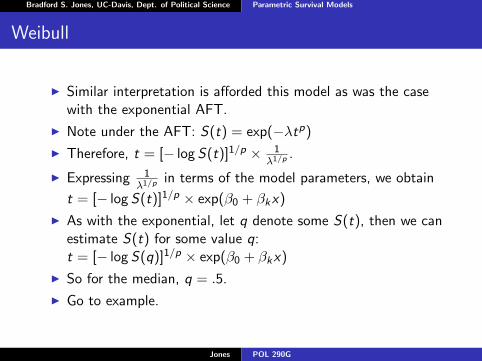
I Similar interpretation is afforded this model as was the casewith the exponential AFT.

I Note under the AFT: S(t) = exp(−λtp)

I Therefore, t = [− log S(t)]1/p × 1λ1/p .

I Expressing 1λ1/p in terms of the model parameters, we obtain

t = [− log S(t)]1/p × exp(β0 + βkx)

I As with the exponential, let q denote some S(t), then we canestimate S(t) for some value q:t = [− log S(q)]1/p × exp(β0 + βkx)

I So for the median, q = .5.

I Go to example.

Jones POL 290G


Log-Logistic

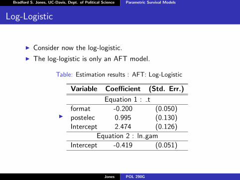
I Consider now the log-logistic.

I The log-logistic is only an AFT model.

Table: Estimation results : AFT: Log-Logistic

I


Equation 1 : t

format -0.200 (0.050)postelec 0.995 (0.130)Intercept 2.474 (0.126)

Equation 2 : ln gam

Intercept -0.419 (0.051)

Jones POL 290G


Jones POL 290G


Log-Logistic

I Consider now the log-logistic.

I The log-logistic is only an AFT model.

I Note that Stata reports γ as the shape parameter.

I This is the inverse of p.

I Consider the survivor function: S(t) = 11+λtp = 1

1+(λ1/pt)p

I Suppose we solve for t: t = [ 1S(t) − 1]1/p × 1

λ1/p

I Express the second term in terms of covariates, we obtain:t = [ 1

S(t) − 1]1/p × exp(β0 + βkx)

I To the example.

Jones POL 290G


Log-Logistic

I Because the log-logistic is AFT and proportional odds, thisratio should be equivalent to the acceleration factor (i.e. theodds ratio exp(β1)).

I So this too is a proportional model . . . in the odds ratios.

I This assumption may not hold.

Jones POL 290G


Many Applications

I These are “plug and play” estimators.

I They are easy to do.

I Let’s run through some illustrations, first in Stata and thenin R

I I use the cabinet duration data.

Jones POL 290G


Weibull

. streg invest polar numst format postelec caretakr, dist(weib) time nolog

failure _d: censor

analysis time _t: durat

Weibull regression -- accelerated failure-time form

No. of subjects = 314 Number of obs = 314

No. of failures = 271

Time at risk = 5789.5

LR chi2(6) = 171.94

Log likelihood = -414.07496 Prob > chi2 = 0.0000

------------------------------------------------------------------------------

_t | Coef. Std. Err. z P>|z| [95% Conf. Interval]

-------------+----------------------------------------------------------------

invest | -.2958188 .1059024 -2.79 0.005 -.5033838 -.0882538

polar | -.017943 .0042784 -4.19 0.000 -.0263285 -.0095575

numst | .4648894 .1005815 4.62 0.000 .2677533 .6620255

format | -.1023747 .0335853 -3.05 0.002 -.1682006 -.0365487

postelec | .6796125 .104382 6.51 0.000 .4750276 .8841974

caretakr | -1.33401 .2017528 -6.61 0.000 -1.729438 -.9385818

_cons | 2.985428 .1281146 23.30 0.000 2.734328 3.236528

-------------+----------------------------------------------------------------

/ln_p | .257624 .0500578 5.15 0.000 .1595126 .3557353

-------------+----------------------------------------------------------------

p | 1.293852 .0647673 1.172939 1.42723

1/p | .7728858 .0386889 .700658 .8525593

Jones POL 290G


Exponential

. streg invest polar numst format postelec caretakr, dist(exp) time nolog

failure _d: censor


Exponential regression -- accelerated failure-time form




LR chi2(6) = 148.53


------------------------------------------------------------------------------


-------------+----------------------------------------------------------------

invest | -.3322088 .1376729 -2.41 0.016 -.6020426 -.0623749

polar | -.0193017 .0055465 -3.48 0.001 -.0301725 -.0084308

numst | .515435 .1291486 3.99 0.000 .2623084 .7685616

format | -.1079432 .0435233 -2.48 0.013 -.1932474 -.022639

postelec | .7403427 .134558 5.50 0.000 .4766138 1.004072

caretakr | -1.319272 .2595422 -5.08 0.000 -1.827965 -.8105783

_cons | 2.944518 .1663401 17.70 0.000 2.618498 3.270539

------------------------------------------------------------------------------

Jones POL 290G


Log-logistic

. streg invest polar numst format postelec caretakr, dist(loglog) time nolog

failure _d: censor


Log-logistic regression -- accelerated failure-time form




LR chi2(6) = 148.72


------------------------------------------------------------------------------


-------------+----------------------------------------------------------------

invest | -.3367541 .1278083 -2.63 0.008 -.5872538 -.0862544

polar | -.0221958 .0052638 -4.22 0.000 -.0325127 -.0118789

numst | .4830709 .1212506 3.98 0.000 .2454241 .7207177

format | -.1093453 .0419715 -2.61 0.009 -.1916078 -.0270827

postelec | .6408808 .1240329 5.17 0.000 .3977807 .8839808

caretakr | -1.26921 .2310272 -5.49 0.000 -1.722015 -.8164046

_cons | 2.728818 .1595866 17.10 0.000 2.416034 3.041602

-------------+----------------------------------------------------------------

/ln_gam | -.5657686 .0511353 -11.06 0.000 -.665992 -.4655451

-------------+----------------------------------------------------------------

gamma | .5679235 .029041 .5137636 .6277928

------------------------------------------------------------------------------

Jones POL 290G


Log-normal

. streg invest polar numst format postelec caretakr, dist(lognorm) time nolog

failure _d: censor


Log-normal regression -- accelerated failure-time form




LR chi2(6) = 150.66


------------------------------------------------------------------------------


-------------+----------------------------------------------------------------

invest | -.3738013 .1327055 -2.82 0.005 -.6338993 -.1137032

polar | -.021988 .0054825 -4.01 0.000 -.0327336 -.0112424

numst | .5717579 .1232281 4.64 0.000 .3302353 .8132805

format | -.1194982 .0432516 -2.76 0.006 -.2042698 -.0347266

postelec | .6668079 .1292366 5.16 0.000 .4135088 .920107

caretakr | -1.126047 .2576962 -4.37 0.000 -1.631122 -.6209713

_cons | 2.632497 .164494 16.00 0.000 2.310095 2.954899

-------------+----------------------------------------------------------------

/ln_sig | .0078719 .0439881 0.18 0.858 -.0783432 .0940871

-------------+----------------------------------------------------------------

sigma | 1.007903 .0443358 .924647 1.098655

Jones POL 290G


Weibull

> cab.weib<-survreg(Surv(durat,censor)~invest + polar + numst +

+ format + postelec + caretakr,data=cabinet,

+ dist=’weibull’)

>

> summary(cab.weib)

Call:

survreg(formula = Surv(durat, censor) ~ invest + polar + numst +

format + postelec + caretakr, data = cabinet, dist = "weibull")

Value Std. Error z p

(Intercept) 2.9854 0.12811 23.30 4.15e-120

invest -0.2958 0.10590 -2.79 5.22e-03

polar -0.0179 0.00428 -4.19 2.74e-05

numst 0.4649 0.10058 4.62 3.80e-06

format -0.1024 0.03359 -3.05 2.30e-03

postelec 0.6796 0.10438 6.51 7.47e-11

caretakr -1.3340 0.20175 -6.61 3.79e-11

Log(scale) -0.2576 0.05006 -5.15 2.65e-07

Scale= 0.773

Weibull distribution

Loglik(model)= -1014.6 Loglik(intercept only)= -1100.6

Chisq= 171.94 on 6 degrees of freedom, p= 0

Number of Newton-Raphson Iterations: 5

n= 314

Jones POL 290G


Log-Logistic

> cab.ll<-survreg(Surv(durat,censor)~invest + polar + numst +


+ dist=’loglogistic’)

>

> summary(cab.ll)

Call:


format + postelec + caretakr, data = cabinet, dist = "loglogistic")


(Intercept) 2.7288 0.15959 17.10 1.50e-65

invest -0.3368 0.12781 -2.63 8.42e-03

polar -0.0222 0.00526 -4.22 2.48e-05

numst 0.4831 0.12125 3.98 6.77e-05

format -0.1093 0.04197 -2.61 9.18e-03

postelec 0.6409 0.12403 5.17 2.38e-07

caretakr -1.2692 0.23103 -5.49 3.93e-08

Log(scale) -0.5658 0.05114 -11.06 1.87e-28

Scale= 0.568

Log logistic distribution

Loglik(model)= -1024.7 Loglik(intercept only)= -1099



n= 314

Jones POL 290G


> ##Log-Normal can be fit using survreg:

>

> cab.ln<-survreg(Surv(durat,censor)~invest + polar + numst +


+ dist=’lognormal’)

>

> summary(cab.ln)

Call:


format + postelec + caretakr, data = cabinet, dist = "lognormal")


(Intercept) 2.63250 0.16449 16.004 1.21e-57

invest -0.37380 0.13271 -2.817 4.85e-03

polar -0.02199 0.00548 -4.011 6.06e-05

numst 0.57176 0.12323 4.640 3.49e-06

format -0.11950 0.04325 -2.763 5.73e-03

postelec 0.66681 0.12924 5.160 2.47e-07

caretakr -1.12605 0.25770 -4.370 1.24e-05

Log(scale) 0.00787 0.04399 0.179 8.58e-01

Scale= 1.01

Log Normal distribution

Loglik(model)= -1025.9 Loglik(intercept only)= -1101.2



n= 314

Jones POL 290G


Comparing Log-Likelihoods (note: non-nested models). I did this in R:

anova(cab.weib, cab.ln, cab.ll)

1 invest + polar + numst + format + postelec + caretakr



Resid. Df -2*LL Test Df Deviance P(>|Chi|)

1 306 2029.238 NA NA NA

2 306 2051.701 = 0 -22.462507 NA

3 306 2049.307 = 0 2.394004 NA

Jones POL 290G


Back to Stata: Generalized Gamma

. streg invest polar numst format postelec caretakr, dist(gamma) nolog

failure _d: censor


Gamma regression -- accelerated failure-time form




LR chi2(6) = 165.78


------------------------------------------------------------------------------


-------------+----------------------------------------------------------------

invest | -.3005269 .108745 -2.76 0.006 -.5136633 -.0873906

polar | -.0182998 .0044674 -4.10 0.000 -.0270559 -.0095438

numst | .4692142 .1030895 4.55 0.000 .2671626 .6712659

format | -.1031368 .0342637 -3.01 0.003 -.1702925 -.0359811

postelec | .6807161 .1061356 6.41 0.000 .4726942 .888738

caretakr | -1.328476 .2066422 -6.43 0.000 -1.733487 -.9234647

_cons | 2.963114 .1447075 20.48 0.000 2.679492 3.246735

-------------+----------------------------------------------------------------

/ln_sig | -.234325 .0802121 -2.92 0.003 -.3915378 -.0771122

/kappa | .9241712 .2065399 4.47 0.000 .5193605 1.328982

-------------+----------------------------------------------------------------

sigma | .7911047 .0634561 .6760165 .9257859

------------------------------------------------------------------------------

Jones POL 290G


Adjudication

I Lots of ChoicesI Selection can be arbitraryI If parametrically nested, standard LR tests apply.I Encompassing Distribution: generalized gamma:

f (t) =λp(λt)pκ−1 exp[−(λt)p]

Γ(κ)(7)

I When κ = 1, the Weibull is implied; when κ = p = 1, theexponential distribution is implied; when κ = 0, thelog-normal distribution is implied; and when p = 1, thegamma distribution is implied.

I In illustrations above, verify that Weibull would be preferredmodel among the choices.

I AIC (−2(log L) + 2(c + p + 1)) also confirms Weibull ispreferred model among choices.

Jones POL 290G


Survivor Functions

Cabinet Duration

0 20 40 60

0

.5

1

Figure: The figure graphs the generalized gamma and Weibull survivorfunctions for the cabinet duration data. The Weibull estimates aredenoted by the “O” symbol and the generalized gamma estimates are

Jones POL 290G


denoted by the line.

Jones POL 290G


Table: AIC and Log-Likelihoods for Cabinet Models

Model Log-Likelihood AICExponential −425.91 865.82Weibull −414.07 844.14Log-Logistic −424.11 864.22Log-Normal −425.31 866.62Gompertz −418.98 853.96Generalized Gamma −414.01 846.02

Jones POL 290G

duration models: parametric models - loginpsfaculty.ucdavis.edu/bsjjones/slide3_parm.pdf ·...

Documents