RESEARCH ARTICLE10.1002/2015WR017752

Dry season streamflow persistence in seasonal climates

David N. Dralle1, Nathaniel J. Karst2, and Sally E. Thompson1

1Department of Civil and Environmental Engineering, University of California, Berkeley, California, USA, 2Division ofMathematics and Science Division, Babson College, Wellesley, Massachusetts, USA

Abstract Seasonally dry ecosystems exhibit periods of high water availability followed by extendedintervals during which rainfall is negligible and streamflows decline. Eventually, such declining flows will fallbelow the minimum values required to support ecosystem functions or services. The time at which dry sea-son flows drop below these minimum values (Q*), relative to the start of the dry season, is termed the‘‘persistence time’’ (TQ� ). The persistence time determines how long seasonal streams can support varioushuman or ecological functions during the dry season. In this study, we extended recent work in the stochas-tic hydrology of seasonally dry climates to develop an analytical model for the probability distributionfunction (PDF) of the persistence time. The proposed model accurately captures the mean of the persist-ence time distribution, but underestimates its variance. We demonstrate that this underestimation arises inpart due to correlation between the parameters used to describe the dry season recession, but that thiscorrelation can be removed by rescaling the flow variables. The mean persistence time predictions formone example of the broader class of streamflow statistics known as crossing properties, which could feasiblybe combined with simple ecological models to form a basis for rapid risk assessment under different climateor management scenarios.

1. Introduction

Pronounced variability in precipitation is the defining characteristic of seasonally dry ecosystems (SDE) [Fati-chi et al., 2012; Vico et al., 2014], which cover nearly 30% of the planet and contain about 30% of the Earth’spopulation [Peel and Finlayson, 2007; CIESIN, 2012]. In these regions, a distinct rainy season is followed by apronounced dry season during which rainfall makes a small or negligible contribution to the water balance.As a consequence, the availability of dry season surface water resources depends strongly on streamflow,which is generated primarily from the storage and subsequent discharge of antecedent wet season rainfallin the subsurface [Brahmananda Rao et al., 1993; Samuel et al., 2008; Andermann et al., 2012]. Because thesetransient stores are strongly influenced by the characteristics of the wet season climate, dry-season wateravailability can be highly variable from year to year in many SDE’s [Samuel et al., 2008; Andermann et al.,2012]. This hydroclimatic variability leaves SDE’s, considered important ‘‘hot spots’’ of biodiversity [Mileset al., 2006; Klausmeyer and Shaw, 2009], and the human populations that depend upon them susceptible tothreats, such as soil erosion, deforestation, and water diversions [Miles et al., 2006; Underwood et al., 2009].Future climate scenarios are projected to further intensify wet season rainfall variability in many SDEs [e.g.,Gao and Giorgi, 2008; Garc�ıa-Ruiz et al., 2011; Dominguez et al., 2012], necessitating models which can pre-dict the response of water resources to climatic change in order to measure the corresponding risk to localecosystems and human populations [Vico et al., 2014; M€uller et al., 2014].

Stochastic methods have a 30 year history of use in deriving simple, process-based models for the probabil-ity distributions of hydrologic variables, such as soil moisture, streamflow, and associated ecologicalresponses [Milly, 1993; Szilagyi et al., 1998; Rodriguez-Iturbe et al., 1999; Laio, 2002; Botter et al., 2007; Thomp-son et al., 2013, 2014]. To date, the majority of stochastic analytical models for hydrology have been devel-oped under conditions where the climatic forcing does not exhibit strong seasonality [Rodriguez-Iturbeet al., 1999; Porporato et al., 2004; Botter et al., 2007]. Those studies that have considered the effects of sea-sonality in rainfall or evaporative demand have either focused on the mean dynamics of the variable ofinterest [Laio, 2002; Feng et al., 2012, 2015] or excluded a treatment of the transient dynamics between thewet and dry seasons [D’odorico et al., 2000; Miller et al., 2007; Kumagai et al., 2009]. This is problematic in

Key Points:� Derived probabilistic model for the

persistence time of dry season highflow conditions� Successfully predicts mean, but not

variance; attributed to inter-annualrecession model variation� Proposed framework for using

crossing statistics (e.g., persistencetime) to forecast ecologic risk

Supporting Information:� Supporting Information S1� Figure S1� Figure S2

Correspondence to:D. N. Dralle,dralle@berkeley.edu

Citation:Dralle, D. N., N. J. Karst, andS. E. Thompson (2015), Dry seasonstreamflow persistence in seasonalclimates, Water Resour. Res., 51,doi:10.1002/2015WR017752.

Received 26 JUN 2015

Accepted 8 DEC 2015

Accepted article online 13 DEC 2015

VC 2015. American Geophysical Union.

All Rights Reserved.

DRALLE ET AL. DRY SEASON STREAMFLOW PERSISTENCE IN SEASONAL CLIMATES 1

Water Resources Research

PUBLICATIONS

situations when such transient hydrologic dynamics have a large impact on the availability of water—i.e., inSDEs [Viola et al., 2008; M€uller et al., 2014; Feng et al., 2015]. Recently, stochastic analytical models forstreamflow and soil moisture have been extended to include seasonal transitions in SDEs [Viola et al., 2008;Feng et al., 2012; M€uller et al., 2014; Feng et al., 2015]. In the case of streamflow models, this is accomplishedby explicitly accounting for the dynamics of the seasonal streamflow recession during the dry season [M€ulleret al., 2014].

In SDE’s, the question, ‘‘how long do dry season streamflows persist above a given level?’’ is highly pertinentto the habitat quality and ecological functions sustained by streams, and to the legal and managementframeworks applied to support those functions. For example, ecosystem managers often assume a corre-spondence between habitat availability and the stream wetted perimeter in order to determine critical min-imum flow values (below which in-stream conditions become suboptimal for habitat protection), [e.g.,Nelson, 1980; Annear and Conder, 1984; Parker and Armstrong, 2001]. These minimum flows are frequentlyadopted as regulatory measures, and thus set conditions beyond which in-stream water abstractions areprohibited. Other ecological transitions are also flow-dependent; for instance, lower bed-shear stresses asso-ciated with low flows are suspected to promote blooms of toxic cyanobacteria in some northern Californiawatersheds [Power et al., 2015] (K. Bouma-Gregson, personal communication, 2015). The flow regime alsoappears to be the primary determinant for temperature-driven stratification of deep river pools, with impli-cations for organisms that depend on these pools for summer survival [Nielsen et al., 1994; Turner andErskine, 2005].

A number of statistical and deterministic modeling methods have been developed to characterize low flowconditions in both gauged and ungauged basins [Nathan and McMahon, 1992; Skøien et al., 2006; M€ullerand Thompson, 2015; Ganora et al., 2009; Castellarin et al., 2007; Laaha and Bl€oschl, 2007; Arnold et al., 1998,among others]. Regression-based and geostatistical techniques employ the concept of hydrologic similar-ity—the idea that catchments with similar geomorphologic and hydroclimatic features should also exhibitsimilar low flow features [Bl€oschl et al., 2013]. Deterministic rainfall-runoff models [e.g., Arnold et al., 1998]can be used for low flow estimation, though such models cannot provide a probabilistic characterizationwithout computationally intensive Monte Carlo techniques.

Compared to their statistical and deterministic counterparts, process-oriented stochastic methods possess anumber of advantages. Their simplicity facilitates applications even when data are sparse, and their mecha-nistic underpinnings overcome the limitations of statistical models which cannot, for example, distinguishbetween the effects of a nonstationary climate and shifts due to land use change. It is also notable thatthese stochastic models typically yield analytic PDF outputs with physically interpretable parameters. Suchexpressions conveniently lend themselves to applications in risk-oriented frameworks. For example, arelated stochastic hydrologic model for soil moisture has been applied to assess plant pathogen risk at theregional scale [Thompson et al., 2013, 2014]. Analogous streamflow methods to estimate ecological risksbased on climate and stream characteristics could provide a toolkit for assessing the condition of existingriverine ecosystems, as well as their vulnerability under alternative climatic, land use, or managementscenarios.

This study aims to develop a model that would support such risk assessment by predicting the probabilisticcharacter of the persistence time. The persistence time, denoted TQ� , is the length of the period that the dryseason streamflow remains above a given flow threshold (Q*). The distribution of TQ� links wet season cli-matic variation and land use (via vegetation water demand) to dry season recession characteristics.

Using the frameworks derived by Botter et al. [2007] and M€uller et al. [2014] to characterize the wet seasonflow dynamics and the transition to the dry season, respectively, we derived analytical expressions for theprobability distribution function (PDF) of TQ� and its expectation. The model is defined for rivers in seasonallydry climates; for this definition to be met, there must be a significant reduction in flow between mean wetseason conditions and the dry season behavior. This condition may be violated in managed rivers (e.g., whendam releases elevate dry season flows) or in watersheds with significant groundwater contributions,which may be sufficient to smooth out flow variations even on seasonal scales. The model was validatedusing a multiyear streamflow data set from the United States Geological Survey’s network of stream gages.

Applying stochastic methods to predict empirical discharge signatures, such as the persistence time, alignswith a recent review of prediction in ungauged basins, which explicitly notes the utility of probabilistic

Water Resources Research 10.1002/2015WR017752

DRALLE ET AL. DRY SEASON STREAMFLOW PERSISTENCE IN SEASONAL CLIMATES 2

streamflow models and calls for more research efforts to characterize their merits and limitations [Bl€oschlet al., 2013]. With this in mind, our model validation demonstrates two important results concerning sto-chastic methods, one ‘‘positive’’ and one ‘‘negative’’:

1. The positive result that the mean persistence time can be identified well as a function of wet season rain-fall statistics and seasonality statistics; allowing the use of analytical models to predict the expected dryseason flow persistence.

2. The negative result that the variance of the persistence time PDF is underestimated, highlighting the sig-nificance of variations in the parameters defining the recession.

We demonstrate that the underestimation of the persistence time variability arises due to fluctuations andcorrelation between the parameters of the power law model used here (and in many other studies, e.g.,Tague and Grant [2004]; Kirchner [2009]; Botter et al. [2009]) to characterize the dry season recession. Thiscorrelation is not physical, but is an inevitable artifact arising from the properties of power laws. Using anexisting power law parameter de-correlation technique [Bergner and Zouhar, 2000; Mather and Johnson,2014], we quantified the effect of this correlation on our predictions, and demonstrated substantialimprovement in the model predictions once it was removed. These simulations motivate further investiga-tion into recession parameter variability; a more thorough understanding of the origins of this behavior iscrucial for the continued development of minimal, process-oriented stochastic models.

2. Methods

2.1. Definition of Symbols and TermsThroughout this section, C �ð Þ represents the gamma function and C �; �ð Þ represents the upper incompletegamma function. The probability density function (PDF) is represented by p and the cumulative densityfunction (CDF) by P. Subscripts, in upper case, denote the random variable being described by the PDF orCDF, and the corresponding lower case characters denote the observed value of the random variable. Forexample, the PDF and the CDF of stream discharge Q at value q are written pQ(q) and PQ(q), respectively.

2.2. Modeling ApproachThe process by which we derive expressions for the mean persistence time and the persistence time proba-bility distribution is illustrated in Figure 1. First, the year is partitioned into a wet and dry season, shown inFigure 1a. The steady state wet season flow PDF (Figure 1b) is obtained from the work of Botter et al. [2007],which is used to derive the probability distribution function describing the streamflow at the start of thedry season/end of the wet season (Figure 1c). This streamflow provides the initial condition for a determinis-tic recession during the dry season, allowing the probability distribution for the initial condition to be trans-formed into a probability distribution for the recession persistence time (Figure 1d). These steps areoutlined in the next sections.2.2.1. Steady State Wet Season Streamflow DistributionThe steady state, wet season streamflow PDF derived by Botter et al. [2007] forms the point of departure forthis analysis. Assuming that recharge events can be described by a marked Poisson process with frequency(k [1/T]) and mean depth (1/cQ, where cQ has units of [T/L3]), and that the catchment residence time distri-bution is also exponential, with mean 1/k [T], the PDF for wet season streamflow (Qw) follows a gammadistribution:

pQw ðqwÞ5cm

Q

CðmÞ qm21w exp 2cQqw

� �: (1)

For an exponential catchment residence time distribution, the streamflow recession is appropriately mod-eled using a linear recession model, dQ/dt 5 –kQ, where k is the inverse of the mean residence time, alsoknown as the streamflow recession constant. Here, the dimensionless parameter m [ ] is the ratio betweenthe mean catchment residence time (1/k [T]) and the mean interarrival time (1/k [T]) of the recharge events.The distribution of recharge depths (exponential with rate parameter cQ) can also be computed from catch-ment soil, vegetation, and hydroclimatic parameters, assumed to be homogeneous across the catchment[Botter et al., 2007; M€uller et al., 2014].

Water Resources Research 10.1002/2015WR017752

DRALLE ET AL. DRY SEASON STREAMFLOW PERSISTENCE IN SEASONAL CLIMATES 3

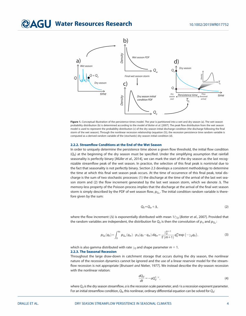
2.2.2. Streamflow Conditions at the End of the Wet SeasonIn order to uniquely determine the persistence time above a given flow threshold, the initial flow condition(Q0) at the beginning of the dry season must be specified. Under the simplifying assumption that rainfallseasonality is perfectly binary [M€uller et al., 2014], we can mark the start of the dry season as the last recog-nizable streamflow peak of the wet season. In practice, the selection of this final peak is nontrivial due tothe fact that seasonality is not perfectly binary. Section 2.3 develops a consistent methodology to determinethe time at which this final wet season peak occurs. At the time of occurrence of this final peak, total dis-charge is the sum of two stochastic processes: (1) the discharge at the time of the arrival of the last wet sea-son storm and (2) the flow increment generated by the last wet season storm, which we denote D. Thememory-less property of the Poisson process implies that the discharge at the arrival of the final wet seasonstorm is simply described by the PDF of wet season flow, pQw . The initial condition random variable is there-fore given by the sum:

Q05Qw1D; (2)

where the flow increment (D) is exponentially distributed with mean 1/cQ [Botter et al., 2007]. Provided thatthe random variables are independent, the distribution for Q0 is then the convolution of pD and pQw :

pQ0ðq0Þ5Z q0

0pQw ðqwÞ � pDðq02qwÞ dqw5

cm11Q

Cðm11Þ qm0 exp 2cQq0

� �; (3)

which is also gamma distributed with rate cQ and shape parameter m 1 1.2.2.3. The Seasonal RecessionThroughout the large draw-down in catchment storage that occurs during the dry season, the nonlinearnature of the recession dynamics cannot be ignored and the use of a linear reservoir model for the stream-flow recession is not appropriate [Brutsaert and Nieber, 1977]. We instead describe the dry-season recessionwith the nonlinear relation:

dQd

dt52aQ12r

d ; (4)

where Qd is the dry season streamflow, a is the recession scale parameter, and r is a recession exponent parameter.For an initial streamflow condition, Q0, this nonlinear, ordinary differential equation can be solved for Qd:

Figure 1. Conceptual illustration of the persistence times model. The year is partitioned into a wet and dry season (a). The wet seasonprobability distribution (b) is determined according to the model of Botter et al. [2007]. The peak flow distribution from the wet seasonmodel is used to represent the probability distribution (c) of the dry season initial discharge condition (the discharge following the finalstorm of the wet season). Through the nonlinear recession relationship (equation (5)), the recession persistence time random variable iscomputed as a derived random variable of the (stochastic) dry season initial condition (d).

Water Resources Research 10.1002/2015WR017752

DRALLE ET AL. DRY SEASON STREAMFLOW PERSISTENCE IN SEASONAL CLIMATES 4

QdðtÞ5ðQr02artÞ

1r : (5)

This form typically well-approximates flow recessions and is supported by multiple theories, which pre-dict that the first-order dynamics of the streamflow recession take a power law form [Brutsaert andNieber, 1977; Harman et al., 2009; Biswal and Marani, 2010]. For most practical cases, the recession expo-nent (1–r) is greater than or equal to one (r � 0) and the units of the recession coefficient (a) depend onthe value of the fitted exponent, which can be determined through empirical fitting procedures or cho-sen from theoretical considerations. These parameters are also known to vary seasonally, interannually,and across individual recession events [Kirchner, 2009; Biswal and Marani, 2010; Botter et al., 2013; Bartand Hope, 2014; Basso et al., 2015]. Section 2.5 examines the potential impact of this form of variabilityon persistence times calculations.2.2.4. The Persistence Time PDF, pTQ� ðtQ� ÞDue to the fact that Q0 can be expressed as a single variable function of tQ� :

Q0ðtQ� Þ5 Qr�1artQ�

� �1r ; (6)

the persistence time PDF (pTQ� ðtQ� Þ) can be obtained as a derived distribution of the dry season initial condi-tion distribution (pQ0ðQ0Þ). Figure 1 illustrates the relationship between Q0 and the persistence time via therecession relationship. By the properties of derived distributions, we find pTQ� ðtQ� Þ as:

pTQ� tQ�ð Þ5pQ0 Q0 tQ�ð Þð ÞdQ0

dt

����tQ�5acm11

Q

C m11ð Þ exp 2cQ Qr�1artQ�

� �1r

h iartQ�1Qr

�� �m2r11

r ; (7)

where 0 < tQ� < 2Qr�=ðarÞ. This positive upper bound on the domain of pTQ� stems from the fact that Q0

!1 as tQ� ! 2Qr�=ðarÞ > 0. In other words, the streamflow recession relationship will always reach the

chosen flow threshold in finite time, even in the limit of an infinitely high initial condition. Since the initialcondition could be less than the chosen flow threshold (Q0 < Q�), the persistence time distribution is alsodefined for all negative real numbers. Nevertheless, as long as the chosen flow threshold value is not unrea-sonably large (less than 50% of the mean annual flow, for example), the proportion of the mass of the per-sistence time PDF associated with negative values for TQ� is negligible. To be precise, the truncation of pTQ�

removes all probability mass for TQ� < 0, which is equal to the probability that the dry season initial condi-tion is less than the chosen flow threshold, Pr TQ� < 0½ �5Pr Q0 < Q�½ �5PQ0 Q�ð Þ. In all subsequent analyses,we truncate pTQ� for TQ� < 0, renormalize the persistence time distribution as 1

12PQ0 Q�ð Þ pTQ� for TQ� > 0, anddo not consider persistence time data for years when Q0 < Q�. In Appendix A, we demonstrate that evenfor relatively high flow thresholds, this condition occurs fewer than 10% of cases.2.2.5. The Mean Persistence Time, E TQ�½ �The direct integration of equation (7) to obtain an expression for the mean persistence time presents ana-lytical difficulties. However, assuming that the peak flow at the end of the wet season exceeds the dry sea-son flow threshold (Q*), equation (6) can be inverted to obtain an expression for tQ� in terms of Q0 and Q*:

Q�5ðQr02artQ� Þ

1r ) tQ�5

Qr02Qr

�ar

: (8)

The expression for tQ� is a function of the random variable, Q0. We can then derive all the moments of thisfunction using the distribution pQ0 . For instance, the mean is given by:

E TQ�½ �5Z 1

Q�

tQ� � pQ0ðQ0Þ dQ0

5

Z 1Q�

Qr02Qr

�a r

�cm11

Q

C m11ð Þ Qm0 exp ð2cQQ0Þ dQ0

5Cðr1m11; cQQ�Þ2ðcQQ�ÞrCðm11; cQQ�Þ

arcrQCðm11Þ :

(9)

While higher order moments, such as the variance, can be obtained, the expressions are unwieldy and arenot presented here.

Water Resources Research 10.1002/2015WR017752

DRALLE ET AL. DRY SEASON STREAMFLOW PERSISTENCE IN SEASONAL CLIMATES 5

2.3. Model Parameter EstimationWe tested the persistence time derivations using U.S. Geological Survey daily discharge data for sixteencatchments in Northern California and Southern Oregon, as detailed in Table 1. These catchments are char-acterized by seasonally dry Mediterranean climates, in which the wet season and the ‘‘growing season’’ (i.e.,summer, with highest insolation and temperature) are out of phase. These catchments exhibit a clear anddramatic separation between flow regimes, and strong seasonal recessions, making them a suitable set ofcatchments on which to test the model. Figure 2 shows the location of the test catchments, along with sitephotos and representative climate data.

Although it is possible to estimate k and cQ from catchment vegetation, soil, and rainfall data, and to inter-polate estimates of the linear recession constant k from neighboring gauges [M€uller and Thompson, 2015],we did not test the persistence time model in ungauged basins. The difference in the quality of parameterestimates for the streamflow model when forced by stream data versus reliable rainfall data were exploredin a previous study, and shown to be minimal [M€uller et al., 2014]. We therefore use gauged streamflowdata to parameterize and to test the model.

To determine the parameters k and cQ, we first identify all well-defined peaks from the wet season hydro-graph (as defined below). k is computed as the reciprocal of the mean of the interarrival periods betweenthese peaks. Next, we extract the magnitude of the increasing segment of the hydrograph preceding eachpeak and compute cQ as the reciprocal of the mean of these positive discharge increments.

The remaining parameters to be estimated are the recession parameters, k for the wet season, and a and r forthe dry season. To estimate these parameters, we first partitioned the year into distinct wet and dry periods.This was achieved by fitting a square wave function to each year of streamflow data, taking a value of themean seasonal streamflow in each case. This fit was constrained by the requirement that the initial guess forthe ‘‘wet season’’ should include both the centroid (along the time axis) of the annual streamflow time series:

sQ5

Z 365

0t � QðtÞdtZ 365

0QðtÞdt

; (10)

and the deviation about the centroid, sQ6sQ, where sQ is defined as the square root of the second momentof the annual streamflow time series:

sQ5

ffiffiffiffiffiffiffiffiffiffiffiffiffiffiffiffiffiffiffiffiffiffiffiffiffiffiffiffiffiffiffiffiffiffiffiffiffiffiffiffiffiffiffiffiZ 365

0t2sQð Þ2 � QðtÞdtZ 365

0QðtÞdt

vuuuuuut : (11)

Table 1. Study Catchment Information

Catchment USGS Gage ID Stream Drainage Area (km2) Years of Data (nj)

C1 11463170 Big Sulphur Creek, Cloverdale, CA 33.9 31C2 11143000 Big Sur River, Big Sur, CA 120.4 60C3 11476600 Bull Creek, Weott, CA 72.8 49C4 14325000 Coquille River, Powers, OR 437.7 81C5 11475000 Eel River, Fort Seward, CA 5457.1 55C6 11475560 Elder Creek, Branscomb, CA 16.8 43C7 11481200 Little River, Trinidad, CA 104.9 49C8 11481000 Mad River, Arcata, CA 1256.1 59C9 11473900 Middle Fork Eel River, Dos Rios, CA 1929.5 45C10 11468000 Navarro River, Navarro, CA 784.8 50C11 11451100 North Fork Cache Creek, Clearlake Oaks, CA 155.9 39C12 11468500 Noyo River, Fort Bragg, CA 274.5 59C13 11472200 Outlet Creek, Longvale, CA 416.0 35C14 11482500 Redwood Creek, Orick, CA 717.4 57C15 11476500 South Fork Eel River, Miranda, CA 1390.8 71C16 14307620 Siuslaw River, Mapleton, CA 1522.9 35

Water Resources Research 10.1002/2015WR017752

DRALLE ET AL. DRY SEASON STREAMFLOW PERSISTENCE IN SEASONAL CLIMATES 6

To estimate the dry season parameters, we first isolated the seasonal recession by identifying the last storm thatinitiated the seasonal dry down. In most cases, this storm was linked to the final streamflow peak in the fitted‘‘wet season’’ square wave. In some cases, however, late spring storms resulted in larger streamflow peaks occur-ring in the initially fitted ‘‘dry season’’ period. The seasonal recession in these cases was taken to begin with thelast of these peaks. The dry season duration (Td) was then defined as the period between the start of the seasonalrecession, and the rising edge of the fitted step function for the following year. Generally, Td exceeded 150 daysin all the study catchments. We used the first Td230 days of the dry season to fit the recession parameters, aand r. The final 30 days were excluded because (i) gauged estimates of extreme low flows typically observed latein the dry season are often unreliable or recorded as zero, and (ii) we wished to exclude the seasonal transitionfrom dry to wet in the fitting procedure to avoid early season storms in the following wet season. An alternativemethod to avoid end of dry season issues would be to fit a and r only to the recession periods greater than thethreshold, Q*. In this case, however, the fitted values a and r may then depend, albeit weakly, on the particularchoice of threshold. This alternative method would undoubtedly generate better model performance, as onlythe relevant portion of the recession time series would be used for fitting. Nevertheless, this study implementsthe first method to ensure fitted values of a and r remain constant, regardless of the choice of threshold.

The wet season recession constant, k, was estimated by extracting all wet season flow recessions exceeding4 days in length, and regressing the logarithm of the recession discharge against time. k was computed asthe median of the regression slope coefficients across all extracted recessions.

The recession parameters (a and r) were fitted using a nonlinear least squares procedure, minimizing thesum of squared errors between the dry season recession model and the observed dry season recessionover all years. Supporting information includes a table of these parameters for each catchment.

Figure 2. Map with study catchments. Insets with monthly averages of high temperature, low temperature, and precipitation totals for the Big Sur River (Big Sur, CA), Elder Creek (Bran-scomb, CA), the North Fork Cache River (Clearlake Oaks, CA), and the Coquille River (Powers, OR).

Water Resources Research 10.1002/2015WR017752

DRALLE ET AL. DRY SEASON STREAMFLOW PERSISTENCE IN SEASONAL CLIMATES 7

2.4. Model EvaluationHaving estimated the model parameters, persistence times were estimated for each year by considering arange of flow thresholds, finding the date at which those thresholds were first crossed during the seasonalrecessions, and computing the time lapsed since the last wet season storm. Persistence times cannot becomputed in this way for two cases:

1. For years when the flow threshold (Q*) exceeded the dry season initial condition (Q0). We do not expectthis restriction to affect the quality of the streamflow data set; even for the highest flow threshold at50% of mean annual flow, this condition accounted for less than 5% of the study years (see Appendix Afor more details).

2. For years when the dry season discharge does not drop below the chosen flow threshold. Unless a riverexplicitly runs dry during the dry season, it will always be possible to define flows so low that the sea-sonal recession does not achieve these levels in a meaningful timeframe, that is, within the duration of atypical dry season.

To ensure that the model is only evaluated for meaningful flow thresholds (namely, flows that are low enoughto be distinct from the wet season, but high enough that the river flow will pass below them in a typical dryseason), we evaluate the model for thresholds (Q*) ranging from 5% to 50% of mean annual flow.

The analytic mean persistence times were plotted against empirical mean persistence times for flow thresh-olds ranging from 5% to 50% of mean annual flow, and the corresponding R2 value of a one-to-one linereported. The performance of the model in estimating persistence time PDFs was evaluated using theNash-Sutcliffe Coefficient (NSC) as applied to the persistence time percentiles:

NSC512

X99

i51Ti 2Ti� �2

X99

j51Tj2

199

X99

k51Tk

� �2 ; (12)

where Ti and Ti are the empirical and modeled persistence times associated with percentile i, respectively.The NSC corresponds to an R2 value for the fit of a one-to-one line to a plot of the empirical percentiles ver-sus the modeled percentiles; it has been used extensively for the assessment of hydrologic models [Nashand Sutcliffe, 1970; Castellarin et al., 2004; M€uller et al., 2014]. NSC values range from negative infinity to one,where an NSC of one corresponds to a perfect match between the percentiles. Due to the strong depend-ence of the persistence times model on the performance of the wet season model, we also computed NSCvalues testing the wet season streamflow distribution (pQw ) and the dry season initial condition distribution(pQ0 ). Although this application of NSC values was originally developed for flow duration curves, the testshere are directly analogous to the duration curve, being derived from the PDFs. We thus assume NSC valuesprovide a suitable relative rating scheme.

Supporting information provides illustrations of the analytic mean persistence times plotted against empiri-cal mean persistence times, and plots of the persistence time PDFs for all catchments with Q* set to 20% ofmean annual flow.

2.5. Effect of Recession Variability on PredictionsAs shown in section 3, the mean persistence time predictions perform well for most watersheds, yet the dis-tributions pTQ� fail to reproduce the variance of the full empirical persistence time distributions. To deter-mine why this occurred, we systematically assessed whether the model assumptions were met by theempirical data. In agreement with other recession studies, we found that the nonlinear recession parame-ters a and r varied significantly between years [Kirchner, 2009; Biswal and Marani, 2010; Shaw and Riha,2012; Botter et al., 2013; Bart and Hope, 2014; Basso et al., 2015]. In violation of the model assumptions,which presume parameter independence, this variation was characterized by a strong correlation betweena and r, which has not been examined in previous recession studies. An example of this correlation is shownfor one of the study sites, Redwood Creek, in Figure 3 (left hand plot).

Such correlation has been identified in other studies as a mathematical artifact that arises from the scale-free properties of the power law (i.e., equation (4)), and existing techniques are available to rescale the flowvariable Q to remove this correlation [Bergner and Zouhar, 2000]. The genesis of this artifact, and the theory

Water Resources Research 10.1002/2015WR017752

DRALLE ET AL. DRY SEASON STREAMFLOW PERSISTENCE IN SEASONAL CLIMATES 8

underpinning its removal, are outlined in Appendix B. The effectiveness of the rescaling technique inremoving the correlation is illustrated in Figure 3 (right hand plot). Two recession curves, which correspondto the two highlighted recession parameter pairs, are plotted in the top of Figure 3. Section 4.1 providesmore background and motivation for the examination of power law parameter correlation. First, however,we outline a method to quantitatively demonstrate the effects of recession parameter variability.2.5.1. Monte Carlo SimulationThe persistence time derivations could be generalized to include recession parameter variability. Thiswould require the specification of a joint PDF for the recession parameters (pA;Rða; rÞ) and the integrationof equation (7), the persistence time distribution, over this joint PDF. While this approach is elegant, thespecification of pA;Rða; rÞ is a serious challenge. Using a – r data to generate an empirical, joint distribu-tion is difficult, considering our small sample sizes (on the order of tens of years of dry season recessiondata per catchment). From a modeling standpoint, the determination of pA;Rða; rÞ from first principleswould require a clear understanding of the mechanisms underlying recession parameter variability, aquestion which remains largely unanswered [Harman et al., 2009], especially when variations in both aand r are considered.

In light of these challenges, we apply a Monte Carlo approach to assess the effects of recession parametervariability and correlation, both separately and in combination, on the predictions of the persistencetime PDF.

To isolate the effects of the recession parameters and their variation, we first fit unique recession curves toeach of the nj observed dry season recessions for catchment j. This process generates nj unique recessionparameters pairs for each catchment, ða1; r1Þ; ða2; r2Þ; . . .; ðanj ; rnj Þ

� . We also compute a set of minimally

correlated recession parameter pairs, denoted a; r, by repeating the fitting procedure to flow data that hadbeen rescaled using the parameter decorrelation method described in Appendix B [Bergner and Zouhar,2000; Mather and Johnson, 2014]. Then, we fit a gamma distribution to the empirical initial conditions Q0 oneach recession. For a given Monte Carlo run, we draw nj samples from this distribution. We use the fitted

Figure 3. Fitted recession parameters for streamflow in units of cfs and dimensionless Q scaled to remove parameter correlation. The two highlighted parameter pairs correspond to thetwo recession curves illustrated in the smaller inset plot.

Water Resources Research 10.1002/2015WR017752

DRALLE ET AL. DRY SEASON STREAMFLOW PERSISTENCE IN SEASONAL CLIMATES 9

rather than the modeled pQ0 PDF in order to confine any model error sources to the treatment of a and rvariation. The Monte Carlo proceeds by drawing a sample of Q0, and computing a persistence time (usingQ* set to 20% mean annual flow). Four different treatments of a and r allow us to assess the effects of a andr variability and correlation on persistence time predictions:

1. M1: constant a and r The original scaling of Q (units of ft3=s) was used. Persistence times were com-puted for each sampled nj initial condition using constant values of a and r. The values of a and r foreach catchment were chosen by minimizing the sum of squared errors between observed and the pre-dicted dry season recessions over all years as described in section 2.3. This is a null case that replicatesthe developments in this paper. It contains neither variability nor correlation in the recession parameters.

2. M2: varying but independent a and r Again, the original scaling of Q in units of ft3=sec is used. In con-trast to M1, the recession parameters are now allowed to vary between each initial condition selected. Therecession parameters are selected by bootstrapping independent samples from the sets a1; a2; . . .; anj

� and r1; r2; . . .; rnj

� . This case preserves variability but does not incorporate the observed correlation in the

recession parameters. Additionally, the results from this simulation provide a reference which can be usedto determine the relative benefit of implementing recession parameter decorrelation (M3).

3. M3: Parameter decorrelation with varying, but independent, a and r . In this instance, Q is rescaledaccording to the decorrelation technique of Bergner and Zouhar [2000]. Persistence times are computedfrom the nj initial conditions using new recession pairs generated by bootstrapping independent sam-ples from the sets a1; a2; . . .; anj

� and r1; r2; . . .; rnj

� . This case preserves variability, and accounts for

the component of correlation in the recession parameters that can be removed by the Bergner andZouhar [2000] method. It is notable that the only difference between M2 and M3 is the scaling of Q. Dif-ferences between the results of M2 and M3 explicitly illustrate the impact of recession parametercorrelation.

4. M4: Parameter decorrelation with varying, jointly sampled a and r pairs. Q is nondimensionlizedaccording to the decorrelation technique of Bergner and Zouhar [2000]. Persistence times are computedfrom the nj initial conditions using recession pairs uniformly sampled (without replacement) fromða1; r1Þ; ða2; r2Þ; . . .; ðanj ; rnj Þ�

. This case preserves variability and all correlation in the recession parame-ters. If the decorrelation procedure completely removed all correlation of the form generated by thescale-dependent artifact (outlined in Appendix B), then there would be no measurable differencesbetween M3 and M4, unless there exists another (physically derived) form of correlation between therecession parameter pairs; that is, correlation that does not obey the form of the artifactual correlation.

For each run of the process, a distribution of persistence times was generated, and compared to the empiri-cal distribution via the NSC. The Monte Carlo process was repeated 1000 times to generate confidenceintervals around the computed NSC’s.

3. Results

3.1. Stochastic Streamflow Model Appliedto Northern California and SouthernOregon CatchmentsThe wet season and dry season initial conditionmodels performed well for the study catch-ments, as shown in Table 2. For the wet seasonmodel, all Nash Sutcliffe coefficients exceeded0.75. With four exceptions (catchments C4, C7,C12, and C14, where 0.5 <NSC< 0.75), thesame holds true for the dry season initial condi-tion. The initial condition models in these fourcatchments overpredicted the magnitude ofthe dry season initial condition.

3.2. Mean Persistence Time and its PDFThe ability of the persistence time model topredict the mean persistence time was good

Table 2. Study Catchment Evaluation Metrics for the Wet SeasonFlow PDF (pQw ), the Dry Season Initial Condition PDF (pQ0 ), and forthe Modeled Mean Persistence Times (E TQ�½ �)Catchment NSC for pQw NSC for pQ0 R2 for E TQ�½ �

C1 0.8 0.94 0.93C2 0.93 0.78 0.41C3 0.89 0.88 0.96C4 0.97 0.71 0.98C5 0.94 0.76 0.88C6 0.88 0.88 0.9C7 0.96 0.58 0.98C8 0.93 0.79 0.95C9 0.81 0.76 0.9C10 0.9 0.9 0.99C11 0.78 0.92 0.85C12 0.9 0.7 0.97C13 0.87 0.8 0.77C14 0.97 0.71 0.96C15 0.91 0.81 0.98C16 0.96 0.81 0.93

Water Resources Research 10.1002/2015WR017752

DRALLE ET AL. DRY SEASON STREAMFLOW PERSISTENCE IN SEASONAL CLIMATES 10

(NSC> 0.75) for discharge thresholds ranging from 5% to 50% of mean annual flow (Table 2). One excep-tion is for catchment C2 (Big Sur), where the model performance is relatively poor.

In Figure 4a, a comparison of the predicted and observed mean persistence times for the threshold range2%–50% of mean annual flow is shown for catchment C14, Redwood Creek. The fit here is typical for mostcatchments, where the mean performance is excellent for larger flow thresholds, and begins to degradeonce the flow threshold approaches 2% mean annual flow (larger persistence times). Generally, mean per-formance across all catchments tends to break down at very low discharge thresholds. As noted in 2.4, thisis because seasonal recessions cannot achieve very low flow thresholds within the dry season duration; thatis, the following wet season begins before the threshold is reached. In this case, persistence times can onlybe computed for the driest years, and so are biased towards smaller values. Catchment C2 (Big Sur) per-forms especially poorly (a breakdown of the model for flow thresholds near 20% of mean annual flow),likely due to the fact that Big Sur has significant geothermal flows generated by three distinct springs. Inthis watershed, dry season flows rarely drop below 20% mean annual flow.

Figure 4a highlights the variability around the mean for both the analytic (gray envelope) and empirical(gray whiskers) mean persistence times. The spread of the analytic curve demonstrates a clear skewtoward shorter persistence times, whereas the empirical curve shows a fairly symmetric spread about themean. Persistence time distributions at 20% of the mean annual flow (blue rectangle in Figure 4a) areplotted in Figure 4b (PDFs at this threshold are presented for all other catchments in supporting informa-tion). At this threshold, it is clear that the analytic persistence time distribution underestimates theobserved variability. Based on the model derived here, moreover, the analytic persistence time distribu-tion is undefined for persistence times outside the interval, 0 < tQ� < 2Qr

�=ðarÞ. The empirical distributiondoes not adhere to this domain restriction. Some of the observed persistence times are more than twiceas large as the maximum possible persistence time predicted by the analytic distribution. Across all flowthresholds and catchments explored here, the modeled persistence time variability underestimates theobserved variability.

Figure 4. The empirical mean persistence time plotted against the analytic mean persistence time for Redwood Creek (a). The gray envelope signifies 95% of the variability around theanalytic mean persistence times, whereas the gray whiskers represent 95% of the variability around the mean empirical persistence times. (b) The full persistence time distribution for adischarge threshold set to 20% of mean annual flow. Blue boxes represent the empirical histogram and the solid black line plots the analytic probability distribution. The empirical(gray-dashed) and analytic (black-dashed) means are also shown in Figure 4b.

Water Resources Research 10.1002/2015WR017752

DRALLE ET AL. DRY SEASON STREAMFLOW PERSISTENCE IN SEASONAL CLIMATES 11

3.3. Source of Persistence Time VariabilityExample persistence time probability distributions generated from a single Monte Carlo run for RedwoodCreek are presented in Figure 5. The results for simulation M1 echo those from the analytic distribution inFigure 4b. As expected, the mean performance is good, but the full variability (Figure 5, empirical data) isnot well accounted for. Simulation M2 represents the case where parameters vary but the correlationbetween pairs is not preserved. In this case, almost all predictive ability is lost. Simulation M3 also relies onindependent bootstrapping of parameters, but the streamflow is scaled (according to the technique ofBergner and Zouhar [2000]) to minimize any recession parameter correlation (specifically, parameter correla-tion that adopts a logarithmic dependence between parameters is eliminated; parameter correlation with adifferent functional dependence may remain). Here the model performance is quite reasonable, and greatlyimproved compared to both M1 and M2. Model M3 does not appear to perform as well as model M4 (whichincludes any correlation remaining after streamflow rescaling), though the difference in performance is notlarge.

These results are general for all the watersheds in the study, as shown in Figure 6. The primary conclusion isthat the greater than expected spread in persistence time distributions results from the coupled interannualvariability in the seasonal recession parameters, a and r. Without accounting for variability in the streamflowrecession parameters (Figure 6, M1), the performances of the analytic PDFs are generally poor, with tightconfidence intervals around the computed NSCs. Simulation M2 demonstrates that neglecting the recessionparameter correlation within a power law model fundamentally violates the mechanics of the power law(such correlation is an inevitable and essential feature of power law functional models, see Appendix B) andleads to basically nonsensical results: poor model performance and wide confidence intervals on the com-puted NSCs. Merely rescaling the flow variables to remove the parameter correlation (M3) greatly improvesmodel performance, although preserving the original recession parameter pairs (M4) continues to improvethe model behavior. Disparities between M3 and M4 indicate that some form of residual parameter correla-tion remains, following the de-correlation procedure. As expected, simulation M4 performs very well, illus-trating that recession parameter pairs are functionally independent of streamflow initial conditions—atleast in terms of the impact on the persistence time PDFs.

4. Discussion

4.1. Model PerformanceThe proposed model for the persistence time during the summer dry season provides a robust estimate ofthe mean conditions at which flow in a drying river is sustained above meaningful threshold values. Themodel thus provides a reasonable basis for estimating the effects of changing climate or land use parame-ters on the mean availability of dry-season surface water resources, and the associated ecosystem servicesthey provide. The minimal parameterization of the model would in principle facilitate distributed assess-ments across many small watersheds.

A full accounting of the variability in dry season streamflow properties clearly requires elucidating the PDFof persistence times, and the analytical model fails to achieve this. Mediocre fits in the dry season initial

Figure 5. Results from a single Monte Carlo run for Redwood Creek. (top row) The blue PDF’s represent the empirical persistence times data, while (bottom row) the multicolored PDF’son the each represent one of the four types of Monte Carlo simulation (M1–M4). The y axis scale is omitted to facilitate comparisons. Also note the scale for MC2, stretched due to thefact that this Monte Carlo simulation produces very large persistence times. NSC values for goodness of fit relative to the empirical persistence times are included for each simulatedprobability distribution.

Water Resources Research 10.1002/2015WR017752

DRALLE ET AL. DRY SEASON STREAMFLOW PERSISTENCE IN SEASONAL CLIMATES 12

condition distribution cannot explain increased variability in the persistence times, unless the distributionsof Q0 themselves exhibited unexpected increases in variability, which they do not. The primary source oferror in the initial condition distributions appears to be a slight bias towards smaller values of Q0. This couldbe due to nonbinary seasonality (bias toward smaller storms toward the end of the wet season), or perform-ance decreases associated with peak flow estimation using the linear recession model in the wet season[Basso et al., 2015]. Monte Carlo simulations illustrate that it is interannual variation in the character of theseasonal recession that results in a large increase in the variability of persistence times, which is not wellestimated with median recession characteristics. Unfortunately, such variation is generally not possible toprescribe a priori.

Physically, variation in recession behavior is thought to arise due to both changes in total catchment stor-age and in the partitioning of that storage amongst reservoirs with different drainage characteristics

Figure 6. Results from the recession parameter Monte Carlo simulations. Each row corresponds to a study catchment, and each columncorresponds to one of the four simulations. Mean Nash-Sutcliffe coefficients are represented with a vertical black line with a color bar cor-responding to the 95% confidence interval of calculated NSC’s; no black line indicates that the mean is less than 21. A red vertical line seg-ment with black circles indicates that the calculated mean NSC and confidence intervals are less than 21. The colorbar scale indicates therelative quality of the fits according to the NSC value.

Water Resources Research 10.1002/2015WR017752

DRALLE ET AL. DRY SEASON STREAMFLOW PERSISTENCE IN SEASONAL CLIMATES 13

[Bart and Hope, 2014; Harman et al., 2009; Biswal and Marani, 2010; Shaw and Riha, 2012; Moore, 1997]. Toaccount for such variability in a lumped model requires specifying multiple reservoirs, each characterizedby distinct timescales—a challenging basis from which to generate stochastic predictions. Fundamentally,the hydrologic literature lacks a unified understanding of the genesis of recession variability, which hasbeen linked by various authors to the drainage dynamics of hillslope aquifers [Brutsaert and Nieber, 1977],to catchment heterogeneity [Harman et al., 2009], and to variability in the wetted extent of the channel net-work [Biswal and Marani, 2010]. Evidently, a single nonlinear reservoir model is inadequate to capture thesevariations and thus to represent the full probabilistic character of seasonal recessions.

Moreover, the parameter correlation identified in this analysis suggests that testing the existing theoriesregarding recession variability requires carefully controlling for the mathematical artifacts that the widelyused power law recession models can generate. Many of the theories addressing recession characteristicsattribute physical meaning to parameters in a power law recession model [Harman et al., 2009; Biswal andMarani, 2010, 2014; Brutsaert and Nieber, 1977]—and yet the values of these parameters, and their relation-ship to each other, appear to be poorly constrained.

As far as we are aware, the mathematical artifact leading to the a – r correlation we observed is systemati-cally removed in only a single study in the hydrological literature: using the technique from Bergner andZouhar [2000], Mather and Johnson [2014] removed power law parameter correlation in order to improvethe performance of a turbidity rating curve. In that work and here, recession parameter correlation pre-sented an unexpected and significant source of model error. In other fields of study, ranging from fluidmechanics to materials science, power law parameter correlation has been mistakenly identified as havingphysical meaning [Zilberstein, 1992; Cortie, 1991; Shih et al., 1990; Hussain et al., 1999]. Power law parametercorrelation has been observed but not properly identified or removed in few streamflow recession studies[Krueger et al., 2010; McMillan et al., 2014; Sawaske and Freyberg, 2014]. This is due, in part, to the fact thatthe classical goal of a recession analysis avoids event-specific recession analyses of a – r point clouds. Never-theless, parameter correlation should be accounted for, where appropriate, especially in light of rapidlyincreasing interest in recession parameter variability [Shaw and Riha, 2012; Bart and Hope, 2014; McMillanet al., 2014; Biswal and Marani, 2014; Basso et al., 2015; Patnaik et al., 2015].

4.2. Ecological Applications of Streamflow Crossing StatisticsThe recession persistence time is one of a more general set of streamflow statistics known as the ‘‘crossingproperties.’’ The crossing properties of hydrologic variables, including soil moisture and streamflow, areknown to be ecologically important [Laio et al., 2001; Porporato et al., 2001; Botter et al., 2008; Doulatyariet al., 2014; Tamea et al., 2011], but their scope of application has been primarily limited to the response ofvegetation to disturbance (e.g., drought, flood, etc).

The persistence of flow above minimum thresholds during the dry season influences many ecological out-comes. For example, low-flow conditions can induce fragmentation of the channel network, impacting themobility of resident stream fishes [Thompson, 1972; Fullerton et al., 2010; Holmes et al., 2015; Hwan and Carl-son, 2015]. As mentioned in the introduction, the seasonal recession in some Northern California water-sheds leads to a fall in the bed shear stress, which can eventually become too low to suppress blooms oftoxic cyanobacteria [Power et al., 2015] (K. Bouma-Gregson, personal communication, 2015). In this case, thepotential for a bloom to occur depends on the persistence time, which, along with the total dry seasonlength, determines the duration of the low flow period during which the bloom can develop.

In addition to these low-flow examples, high-flows can also initiate important ecological processes, forinstance by submerging fish passage obstacles [Reiser et al., 2011; Holmes et al., 2015] and allowing migra-tions to extend into the upper reaches of watersheds; or by causing scouring of the stream bed. Taking theEel River as an example again, observations suggest that bankfull flows mobilize enough sediment to dis-lodge or crush algae-grazing macroinvertebrates. This scour and associated loss of grazers promotes largedry season blooms of filamentous green algae, forming the structural backbone of dry season food websthat support salmonid fishes [Power et al., 2008]. The sequence of whether these thresholds are crossed ornot during wet seasons and successive dry seasons can lead to substantially different ecological states[Power et al., 2015]. These situations should be readily amenable to stochastic analysis and incorporationinto risk-based predictive frameworks.

Water Resources Research 10.1002/2015WR017752

DRALLE ET AL. DRY SEASON STREAMFLOW PERSISTENCE IN SEASONAL CLIMATES 14

5. Conclusion

This study developed a probabilisticmodel of the persistence time, TQ� , thenumber of days from the start of thedry season for which dry season flowexceeds Q*. By linking the dry seasonrecession to wet season flow dynamicsthrough a dry season initial conditionmodel (pQ0 ), the model analyticallydemonstrates the precise linkagesbetween the dry season recession andsimple measures of wet season hydro-climate and catchment geomorphol-ogy. In spite of excellent performancein the mean sense, the model did not

incorporate an unexpected but essential source of variability: interannual fluctuations in the recessionbehavior, and correlation between the parameters used to describe it. The positive performance of themodel overall suggests the potential for future work to exploit hydrologic predictions of the crossing prop-erties of wet and dry season flows to support large-scale, rapid, in-stream ecological risk assessments. Thechallenges associated with capturing variability in seasonal recessions demonstrate the importance ofimproving understanding of recession variability. Parameter decorrelation emerges as a promising researchavenue to separate the informative characteristics of hydrograph recessions from those that are purelyattributable to the mathematical properties of the widely used power law model.

Appendix A: Resolving the Issue of Negative Persistence Times

It is possible that the dry season initial condition could be less than the flow threshold, (Q0<Q*). In this case,the model will predict a negative persistence time. To resolve this issue, we discard years for which Q0<Q* andtruncate all negative values in the persistence time PDF. For even reasonably high flow thresholds, this conditionis true for only a small fraction of the years considered. With the flow threshold set at 50% of mean wet seasonflow E Qw½ �5m=ð2cQÞ

� �, which will be considerably higher than 50% of mean annual flow, this probability can

be computed exactly using the cumulative distribution function of the dry season initial condition:

Pr TQ� < 0½ �5Pr Q0 < Q�½ �5PQ0

m2cQ

�512

C m11;m2

� �Cðm11Þ : (A1)

Figure 7 plots this probability across a broad range of realistic values for m. The maximum probabilityoccurs for m 5 1, and even in this case, Q0<Q* is expected to occur less than 10% of the time, even for thisrelatively high flow threshold. Therefore, discarding years with Q0<Q* will not significantly affect the qual-ity of computed persistence time data.

Appendix B: Recession Parameter Correlation

The strong log-linear correlative relationship between the a and r parameters can be directly traced to thechoice of a power law recession model: dQ

dt 52aQ12r [Bergner and Zouhar, 2000]. This particular form ofscale-dependent, artifactual correlation can be deliberately minimized through rescaling of the flow vari-able. Bergner and Zouhar [2000] analytically construct the scaling constant (Q! Q=Qscale):

Qscale5102

Pnj

i51ð�r2riÞlog ai=agð ÞPnj

i51 �r2rið Þ2

!; (B1)

to force the linear correlation coefficient between log a and r to equal zero. Each Qscale will be unique for agiven catchment and is computed using the nj fitted recession parameters, the mean of the ri’s (�r ), and thegeometric mean of the ai’s (ag). Fitting recession curves to these new, rescaled recessions will yield a newset of nj unique recession parameter pairs, ða1; r1Þ; ða2; r2Þ; . . .; ðanj ; rnj Þ

� .

Figure 7. Probability that the dry season initial condition (Q0) is less than a flowthreshold set to 50% of the mean wet season flows for a range of realistic valuesof m.

Water Resources Research 10.1002/2015WR017752

DRALLE ET AL. DRY SEASON STREAMFLOW PERSISTENCE IN SEASONAL CLIMATES 15

ReferencesAndermann, C., L. Longuevergne, S. Bonnet, A. Crave, P. Davy, and R. Gloaguen (2012), Impact of transient groundwater storage on the

discharge of Himalayan rivers, Nat. Geosci., 5(2), 127–132, doi:10.1038/ngeo1356.Annear, T. C., and A. L. Conder (1984), Relative bias of several fisheries instream flow methods, N. Am. J. Fish. Manage., 4, 531–539,

doi:10.1577/1548-8659(1984)4<531:RBOSFI>2.0.CO;2.Arnold, J. G., R. Srinivasan, R. S. Muttiah, and J. R. Williams (1998), Large area hydrologic modeling and assessment part i: Model develop-

ment, J. Am. Water Resour. Assoc., 34(1), 73–89.Bart, R., and A. Hope (2014), Inter-seasonal variability in baseflow recession rates: The role of aquifer antecedent storage in central

California watersheds, J. Hydrol., 519, 205–213, doi:10.1016/j.jhydrol.2014.07.020.Basso, S., M. Schirmer, and G. Botter (2015), On the emergence of heavy-tailed streamflow distributions, Adv. Water Resour., 82, 98–105.Bergner, F., and G. Zouhar (2000), A new approach to the correlation between the coefficient and the exponent in the power law equation

of fatigue crack growth, Int. J. Fatigue, 22(3), 229–239.Biswal, B., and M. Marani (2010), Geomorphological origin of recession curves, Geophys. Res. Lett., 37, L24403, doi:10.1029/2010GL045415.Biswal, B., and M. Marani (2014), Universal’ recession curves and their geomorphological interpretation, Adv. Water Resour., 65, 34–42, doi:

10.1016/j.advwatres.2014.01.004.Bl€oschl, G., M. Sivapalan, and T. Wagener (2013), Runoff Prediction in Ungauged Basins: Synthesis Across Processes, Places and Scales, Cam-

bridge Univ. Press, Cambridge, England.Botter, G., A. Porporato, I. Rodriguez-Iturbe, and A. Rinaldo (2007), Basin-scale soil moisture dynamics and the probabilistic characterization

of carrier hydrologic flows: Slow, leaching-prone components of the hydrologic response, Water Resour. Res., 43, W02417, doi:10.1029/2006WR005043.

Botter, G., S. Zanardo, A. Porporato, I. Rodr�ıguez-Iturbe, and A. Rinaldo (2008), Ecohydrological model of flow duration curves and annualminima, Water Resour. Res., 44, W08418, doi:10.1029/2008WR006814.

Botter, G., A. Porporato, I. Rodr�ıguez-Iturbe, and A. Rinaldo (2009), Nonlinear storage-discharge relations and catchment streamflowregimes, Water Resour. Res., 45, W10427, doi:10.1029/2008WR007658.

Botter, G., S. Basso, I. Rodriguez-Iturbe, and A. Rinaldo (2013), Resilience of river flow regimes, Proc. Natl. Acad. Sci. U. S. A., 110(32),12,925–12,930.

Brahmananda Rao, V., M. C. de Lima, and S. H. Franchito (1993), Seasonal and interannual variations of rainfall over eastern northeast Brazil,J. Clim., 6(9), 1754–1763, doi:10.1175/1520-0442(1993)006<1754:SAIVOR>2.0.CO;2.

Brutsaert, W., and J. L. Nieber (1977), Regionalized drought flow hydrographs from a mature glaciated plateau, Water Resour. Res., 13(3),637–643, doi:10.1029/WR013i003p00637.

Castellarin, A., G. Galeati, L. Brandimarte, A. Montanari, and A. Brath (2004), Regional flow-duration curves: Reliability for ungauged basins,Adv. Water Resour., 27(10), 953–965.

Castellarin, A., G. Camorani, and A. Brath (2007), Predicting annual and long-term flow-duration curves in ungauged basins, Adv. WaterResour., 30(4), 937–953.

CIESIN (2012), National Aggregates of Geospatial Data Collection: Population, Landscape, And Climate Estimates, Version 3 (PLACE III), NASA,Socioecon. Data and Appl. Cent., N. Y., doi:10.7927/H4F769GP.

Cortie, M. B. (1991), The irrepressable relationship between the Paris law parameters, Eng. Fract. Mech., 40(3), 681–682, doi:10.1016/0013-7944(91)90160-3.

D’odorico, P., L. Ridolfi, A. Porporato, and I. Rodriguez-Iturbe (2000), Preferential states of seasonal soil moisture: The impact of climate fluc-tuations, Water Resour. Res., 36(8), 2209–2219, doi:10.1029/2000WR900103.

Dominguez, F., E. Rivera, D. P. Lettenmaier, and C. L. Castro (2012), Changes in winter precipitation extremes for the western United Statesunder a warmer climate as simulated by regional climate models, Geophys. Res. Lett., 39, L05803, doi:10.1029/2011GL050762.

Doulatyari, B., S. Basso, M. Schirmer, and G. Botter (2014), River flow regimes and vegetation dynamics along a river transect, Adv. WaterResour., 73, 30–43, doi:10.1016/j.advwatres.2014.06.015.

Fatichi, S., V. Y. Ivanov, and E. Caporali (2012), Investigating interannual variability of precipitation at the global scale: Is there a connectionwith seasonality?, J. Clim., 25(16), 5512–5523, doi:10.1175/JCLI-D-11-00356.1.

Feng, X., G. Vico, and A. Porporato (2012), On the effects of seasonality on soil water balance and plant growth, Water Resour. Res., 48,W05543, doi:10.1029/2011WR011263.

Feng, X., A. Porporato, and I. Rodr�ıguez-Iturbe (2015), Stochastic soil water balance under seasonal climates, Proc. R. Soc. A, 471(2174), doi:10.1098/rspa.2014.0623.

Fullerton, A. H., K. M. Burnett, E. A. Steel, R. L. Flitcroft, G. R. Pess, B. E. Feist, C. E. Togersen, D. J. Miller, and B. L. Sanderson (2010), Hydrolog-ical connectivity for riverine fish: Measurement challenges and research opportunities, Freshwater Biol., 55(11), 2215–2237, doi:10.1111/j.1365-2427.2010.02448.x.

Ganora, D., P. Claps, F. Laio, and A. Viglione (2009), An approach to estimate nonparametric flow duration curves in ungauged basins,Water Resour. Res., 45, W10418, doi:10.1029/2008WR007472.

Gao, X., and F. Giorgi (2008), Increased aridity in the Mediterranean region under greenhouse gas forcing estimated from high resolutionsimulations with a regional climate model, Global Planet. Change, 62(3–4), 195–209, doi:10.1016/j.gloplacha.2008.02.002.

Garc�ıa-Ruiz, J. M., J. I. L�opez-Moreno, S. M. Vicente-Serrano, T. Lasanta Mart�ınez, and S. Beguer�ıa (2011), Mediterranean water resources in aglobal change scenario, Earth Sci. Rev., 105(3–4), 121–139, doi:10.1016/j.earscirev.2011.01.006.

Harman, C. J., M. Sivapalan, and P. Kumar (2009), Power law catchment-scale recessions arising from heterogeneous linear small-scaledynamics, Water Resour. Res., 45, W09404, doi:10.1029/2008WR007392.

Holmes, R. W., D. E. Rankin, E. Ballard, and M. Gard (2015), Evaluation of Steelhead passage flows using hydraulic modeling on an unregu-lated coastal California River, River Res. Appl., doi:10.1002/rra.2884, in press.

Hussain, M. A., S. Kar, and R. R. Puniyani (1999), Relationship between power law coefficients and major blood constituents affecting thewhole blood viscosity, J. Biosci., 24(3), 329–337, doi:10.1007/BF02941247.

Hwan, J. L., and S. M. Carlson (2015), Fragmentation of an intermittent stream during seasonal drought: Intra-annual and interannual pat-terns and biological consequences, River Res. Appl., doi:10.1002/rra.2907, in press.

Kirchner, J. W. (2009), Catchments as simple dynamical systems: Catchment characterization, rainfall-runoff modeling, and doing hydrologybackward, Water Resour. Res., 45, W02429, doi:10.1029/2008WR006912.

Klausmeyer, K. R., and M. R. Shaw (2009), Climate change, habitat loss, protected areas and the climate adaptation potential of species inmediterranean ecosystems worldwide, PLoS One, 4, doi:10.1371/journal.pone.0006392.

AcknowledgmentsD. Dralle thanks the NSF GRFP.S.E. Thompson acknowledges supportfrom NSF EAR-1331940. The authorswould like to thank Suzanne Kelsonfrom the Eel River Critical ZoneObservatory for her images of ElderCreek, and Stephanie Carlson from theEnvironmental Science, Management,and Policy department at UC Berkeleyfor her edits and discussions regardingpossible ecological applications of thiswork. All the streamflow data used forthis study can be found on the websitefor United States Geological Survey(http://waterdata.usgs.gov/nwis).

Water Resources Research 10.1002/2015WR017752

DRALLE ET AL. DRY SEASON STREAMFLOW PERSISTENCE IN SEASONAL CLIMATES 16

Krueger, T., J. Freer, J. N. Quinton, C. J. A. Macleod, G. S. Bilotta, R. E. Brazier, P. Butler, and P. M. Haygarth (2010), Ensemble evaluation ofhydrological model hypotheses, Water Resour. Res., 46, W07516, doi:10.1029/2009WR007845.

Kumagai, T., N. Yoshifuji, and N. Tanaka (2009), Comparison of soil moisture dynamics between a tropical rain forest and a tropical seasonalforest in southeast Asia: Impact of seasonal and year-to-year variations in rainfall, Water Resour. Res., 45, W04413, doi:10.1029/2008WR007307.

Laaha, G., and G. Bl€oschl (2007), A national low flow estimation procedure for Austria, Hydrol. Sci. J., 52(4), 625–644.Laio, F. (2002), On the seasonal dynamics of mean soil moisture, J. Geophys. Res., 107(D15), 4272, doi:10.1029/2001JD001252.Laio, F., A. Porporato, L. Ridolfi, and I. Rodriguez-Iturbe (2001), Mean first passage times of processes driven by white shot noise, Phys. Rev.

E, 63(3), 036105, doi:10.1103/PhysRevE.63.036105.Mather, A. L., and R. L. Johnson (2014), Quantitative characterization of stream turbidity-discharge behavior using event loop shape model-

ing and power law parameter decorrelation, Water Resour. Res., 50, 7766–7779, doi:10.1016/S0142-1123(99)00123-1.McMillan, H., M. Gueguen, E. Grimon, R. Woods, M. Clark, and D. E. Rupp (2014), Spatial variability of hydrological processes and model

structure diagnostics in a 50km2 catchment, Hydrol. Processes, 28(18), 4896–4913, doi:10.1002/hyp.9988.Miles, L., A. C. Newton, R. S. DeFries, C. Ravilious, I. May, S. Blyth, V. Kapos, and J. E. Gordon (2006), A global overview of the conservation

status of tropical dry forests, J. Biogeogr., 33(3), 491–505, doi:10.1111/j.1365-2699.2005.01424.x.Miller, G. R., D. D. Baldocchi, B. E. Law, and T. Meyers (2007), An analysis of soil moisture dynamics using multi-year data from a network of

micrometeorological observation sites, Adv. Water Resour., 30, 1065–1081, doi:10.1016/j.advwatres.2006.10.002.Milly, P. C. D. (1993), An analytic solution of the stochastic storage problem applicable to soil water, Water Resour. Res., 29(11), 3755–3758,

doi:10.1029/93WR01934.Moore, R. D. (1997), Storage-outflow modelling of streamflow recessions, with application to a shallow-soil forested catchment, J. Hydrol.,

198, 260–270, doi:10.1016/S0022-1694(96)03287-8.M€uller, M. F., and S. E. Thompson (2015), A topological restricted maximum likelihood (TopREML) approach to regionalize trended runoff

signatures in stream networks, Hydrol. Earth Syst. Sci. Discuss., 12(1), 1355–1396, doi:10.5194/hessd-12-1355-2015.M€uller, M. F., D. N. Dralle, and S. E. Thompson (2014), Analytical model for flow duration curves in seasonally dry climates, Water Resour.

Res., 50, 5510–5531, doi:10.1002/2014WR015301.Nash, J. E., and J. V. Sutcliffe (1970), River flow forecasting through conceptual models part I: A discussion of principles, J. Hydrol., 10(3),

282–290, doi:10.1016/0022-1694(70) 90255-6.Nathan, R. J., and T. A. McMahon (1992), Estimating low flow characteristics in ungauged catchments, Water Resour. Manage., 6(2), 85–100.Nelson, F. A. (1980), Evaluation of Four Instream Flow Methods Applied to Four Trout Rivers in Southwest Montana, Mont. Dep. of Fish

Wildlife and Parks, Helena, Montana, doi:10.5962/bhl.title. 23324.Nielsen, J. L., T. E. Lisle, and V. Ozaki (1994), Thermally stratified pools and their use by steelhead in northern California streams, Trans. Am.

Fish. Soc., 123, 613–626, doi:10.1577/1548-8659(1994)123<0613:TSPATU>2.3.CO;2.Parker, G. W., and D. S. Armstrong (2001), Preliminary assessment of streamflow requirements for habitat protection for selected sites on

the Assabet and Charles Rivers, eastern Massachusetts, U.S. Geol. Surv. Open-File Rep., 02-340, 35 p.Patnaik, S., B. Biswal, D. N. Kumar, and B. Sivakumar (2015), Effect of catchment characteristics on the relationship between past discharge

and the power law recession coefficient, J. Hydrol., 528, 321–328.Peel, M. C., and B. L. Finlayson (2007), Updated world map of the K€oppen-Geiger climate classification, Hydrol. Earth Syst. Sci., 4, 439–473,

doi:10.5194/hess-11-1633-2007.Porporato, A., F. Laio, L. Ridolfi, and I. Rodriguez-Iturbe (2001), Plants in water-controlled ecosystems: Active role in hydrologic processes

and response to water stress: III. Vegetation water stress, Adv. Water Resour., 24(7), 725–744, doi:10.1016/S0309-1708(01)00006-9.Porporato, A., E. Daly, and I. Rodr�ıguez-Iturbe (2004), Soil water balance and ecosystem response to climate change, Am. Nat., 164(5),

625–632, doi:10.1086/424970.Power, M. E., M. S. Parker, and W. E. Dietrich (2008), Seasonal reassembly of a river food web: Floods, droughts, and impacts of fish, Ecol.

Monogr., 78(2), 263–282, doi:10.1890/06-0902.1.Power, M. E., K. Bouma-Gregson, P. Higgins, and S. M. Carlson (2015), The thirsty eel: Summer and winter flow thresholds that tilt the eel river

of northwestern California from salmon-supporting to cyanobacterially degraded states, Copeia, 2015(1), 200–211, doi:10.1643/CE-14-086.Reiser, D. W., C. Huang, S. Beck, M. Gagner, and E. Jeanes (2011), Defining flow windows for upstream passage of adult anadromous salmo-

nids at Cascades and Falls, Trans. Am. Fish. Soc., 135(3), 668–679, doi:10.1577/T05-169.1.Rodriguez-Iturbe, I., A. Porporato, L. Ridolfi, V. Isham, and D. R. Coxi (1999), Probabilistic modelling of water balance at a point: The role of

climate, soil and vegetation, Proc. R. Soc. A, 455(1990), 3789–3805, doi:10.1098/rspa.1999.0477.Samuel, J. M., M. Sivapalan, and I. Struthers (2008), Diagnostic analysis of water balance variability: A comparative modeling study of catch-

ments in Perth, Newcastle, and Darwin, Australia, Water Resour. Res., 44, W06403, doi:10.1029/2007WR006694.Sawaske, S. R., and D. L. Freyberg (2014), An analysis of trends in baseflow recession and low-flows in rain-dominated coastal streams of

the pacific coast, J. Hydrol., 519, 599–610.Shaw, S. B., and S. J. Riha (2012), Examining individual recession events instead of a data cloud: Using a modified interpretation of dQ/

dt–Q streamflow recession in glaciated watersheds to better inform models of low flow, J. Hydrol., 434-435, 46–54, doi:10.1016/j.jhydrol.2012.02.034.

Shih, W., M. Orlowski, and K. Y. Fu (1990), Parameter correlation and modeling of the power-law relationship in mosfet hot-carrier degrada-tion, IEEE Elect. Device Lett., 11(7), 297–299, doi:10.1109/55.56480.

Skøien, J. O., R. Merz, and G. Bl€oschl (2006), Top-kriging-geostatistics on stream networks, Hydrol. Earth Syst. Sci., 10(2), 277–287.Szilagyi, J., M. B. Parlange, and J. D. Albertson (1998), Recession flow analysis for aquifer parameter determination, Water Resour. Res., 34(7),

1851–1857, doi:10.1029/98WR01009.Tague, C., and G. E. Grant (2004), A geological framework for interpreting the low-flow regimes of Cascade streams, Willamette River Basin,

Oregon, Water Resour. Res., 40, W04303, doi:10.1029/2003WR002629.Tamea, S., F. Laio, L. Ridolfi, and I. Rodriguez-Iturbe (2011), Crossing properties for geophysical systems forced by Poisson noise, Geophys.

Res. Lett., 38, L18404, doi:10.1029/2011GL049074.Thompson, K. (1972), Determining stream flows for fish life, Pacific Northwest River Basins Commission, In stream Flow Requirement Work-

shop, The Commission, Portland, Oreg.Thompson, S., S. Levin, and I. Rodr�ıguez-Iturbe (2013), Linking plant disease risk and precipitation drivers: A dynamical systems framework,

Am. Nat., 181(1), E1–E16, doi:10.1086/668572.Thompson, S. E., S. Levin, and I. Rodr�ıguez-Iturbe (2014), Rainfall and temperatures changes have confounding impacts on Phytophthora cinna-

momi occurrence risk in the southwestern USA under climate change scenarios, Global Change Biol., 20(4), 1299–1312, doi:10.1111/gcb.12463.

Water Resources Research 10.1002/2015WR017752

DRALLE ET AL. DRY SEASON STREAMFLOW PERSISTENCE IN SEASONAL CLIMATES 17

Turner, L., and W. D. Erskine (2005), Variability in the development, persistence and breakdown of thermal, oxygen and salt stratificationon regulated rivers of Southeastern Australia, River Res. Appl., 21, 151–168, doi:10.1002/rra.838.

Underwood, E. C., J. H. Viers, K. R. Klausmeyer, R. L. Cox, and M. R. Shaw (2009), Threats and biodiversity in the mediterranean biome, Divers.Distrib., 15(2), 188–197, doi:10.1111/j.1472-4642.2008.00518.x.

Vico, G., et al. (2014), Climatic, ecophysiological, and phenological controls on plant ecohydrological strategies in seasonally dry ecosys-tems, Ecohydrology, 8, 660–681, doi:10.1002/eco.1533.

Viola, F., E. Daly, G. Vico, M. Cannarozzo, and A. Porporato (2008), Transient soil-moisture dynamics and climate change in mediterraneanecosystems, Water Resour. Res., 44, W11412, doi:10.1029/2007WR006371.

Zilberstein, V. A. (1992), On correlations between the power law parameters, Int. J. Fract., 58(3), R57–R59, doi:10.1007/BF00015624.

Water Resources Research 10.1002/2015WR017752

DRALLE ET AL. DRY SEASON STREAMFLOW PERSISTENCE IN SEASONAL CLIMATES 18