DRIPs and the Dividend Pay Date Effect

September 2013

Henk Berkman

University of Auckland Business School

Auckland, New Zealand

h.berkman@auckland.ac.nz

Paul D. Koch*

School of Business

University of Kansas

Lawrence, KS 66045

pkoch@ku.edu

*Corresponding author. This version is preliminary. We acknowledge the helpful comments of

Ferhat Akbas, Robert DeYoung, David Emanuel, Kathleen Fuller, Brad Goldie, Ted Juhl, Michal

Kowalik, Joe Lan, Dimitris Margaritis, Alastair Marsden, Felix Meschke, Nada Mora, Peter

Phillips, David Solomon, Ken Spong, Jide Wintoki, and seminar participants at the Annual

Conferences of the Society of Financial Studies Finance Cavalcade, the Financial Management

Association, and the Southern Finance Association, as well as the University of Auckland, the

University of Canterbury, the University of Kansas, and the Federal Reserve Bank of Kansas

City. We also acknowledge the excellent research assistance of Aaron Andra, Suzanna Emelio,

and Evan Richardson. Please do not quote without permission.

2

DRIPs and the Dividend Pay Date Effect

Abstract

On the day that dividends are paid we find a significant positive abnormal return that is

completely reversed over the following days. This dividend pay date effect has strengthened

since the 1970s, and is concentrated among high dividend yield stocks that offer dividend

reinvestment plans (DRIPs). It is larger for DRIP stocks that face greater limits to arbitrage and

for stocks with greater participation in their DRIPs. Profits from a trading strategy that exploits

this price behavior are economically significant, and are correlated with market sentiment,

transaction costs, the dividend premium, and the VIX.

JEL Classification: D82, G14, G19.

Key Words: market efficiency, anomaly, dividend reinvestment plan, retail investors, sentiment,

transaction costs, short sales, institutional ownership.

1

I. Introduction

Many studies examine stock prices around the dividend announcement day or the ex-

dividend date. These events might contain value-relevant news associated with a dividend

surprise, or evoke trading to capture dividends.1 In contrast, when the dividend pay date arrives,

there is no tax-motivated trading and no new information about the amount or timing of this

distribution. Nevertheless, we find striking evidence of a predictable price increase around the

pay date that is completely reversed over the following days. This temporary inflation is

concentrated among firms with a high dividend yield and dividend reinvestment plans (DRIPs).2

The fact that there is no new information on the pay date, combined with the prevalence

of DRIPs among U.S. stocks, creates an ideal setting to test the price pressure hypothesis.3

Ogden (1994) is the first to exploit these features, and examines the dividend pay date effect for

U.S. stocks during the period, 1962 - 1989. He finds a small but significant mean abnormal

return of 7 basis points (bp) on the pay date, which accumulates to 20 bp over the following three

days. However, he finds no significant price reversal after the pay date, and thus concludes that

his evidence does not support the temporary price pressure hypothesis.

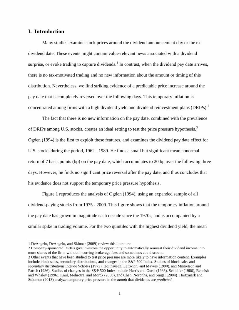
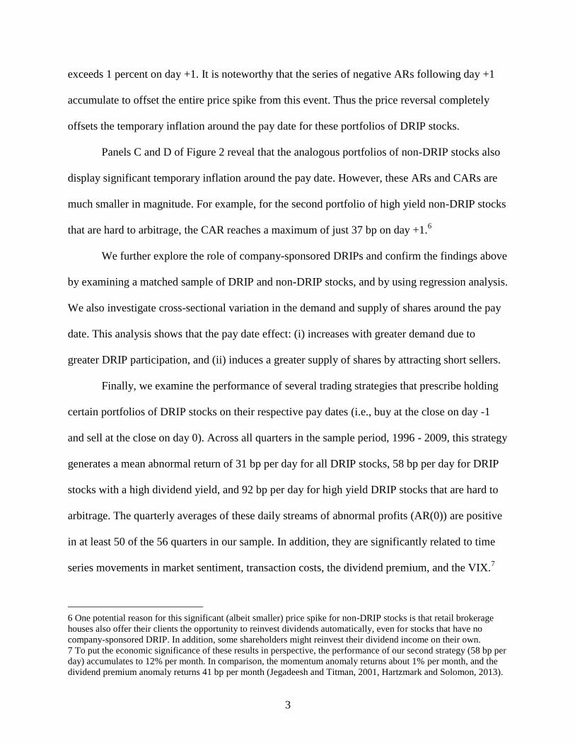
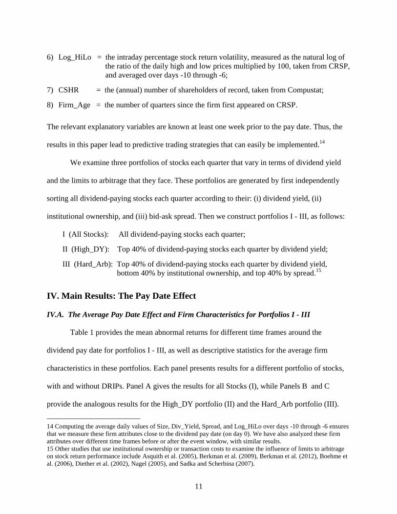
Figure 1 reproduces the analysis of Ogden (1994), using an expanded sample of all

dividend-paying stocks from 1975 - 2009. This figure shows that the temporary inflation around

the pay date has grown in magnitude each decade since the 1970s, and is accompanied by a

similar spike in trading volume. For the two quintiles with the highest dividend yield, the mean

1 DeAngelo, DeAngelo, and Skinner (2009) review this literature.

2 Company-sponsored DRIPs give investors the opportunity to automatically reinvest their dividend income into

more shares of the firm, without incurring brokerage fees and sometimes at a discount.

3 Other events that have been studied to test price pressure are more likely to have information content. Examples

include block sales, secondary distributions, and changes in the S&P 500 Index. Studies of block sales and

secondary distributions include Scholes (1972), Holthausen, Leftwich, and Mayers (1990), and Mikkelson and

Partch (1986). Studies of changes in the S&P 500 Index include Harris and Gurel (1986), Schleifer (1986), Beneish

and Whaley (1996), Kaul, Mehrotra, and Morck (2000), and Chen, Noronha, and Singal (2004). Hartzmark and

Solomon (2013) analyze temporary price pressure in the month that dividends are predicted.

2

abnormal return on the pay date (AR(0)) has increased from 12 bp in the 1970s (Panel A) to 40

bp in the first decade of the new millennium (Panel D). This recent decade also reveals several

significant negative price spikes after day +1, indicating a reversal that offsets the temporary

inflation. In addition, for the recent decade, we find a significant price spike on day -3,

suggesting that some shareholders may buy additional shares three days before the pay date, and

pay for these shares with the dividend income received on day 0 (Odgen, 1994, Yadav, 2010).4

The main goal of this paper is to explore how the pay date effect varies across stocks,

with a particular emphasis on the role of company-sponsored DRIPs. We extend the analysis of

Ogden by separately analyzing the behavior of DRIP firms versus non-DRIP firms during the

period from 1996 through 2009. We focus on this recent period because it reveals the greatest

price pressure in Figure 1, and because we have lists of firms with DRIPs for this time frame.

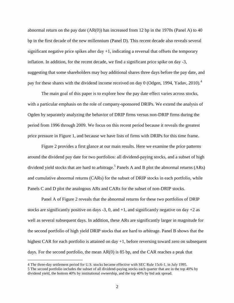
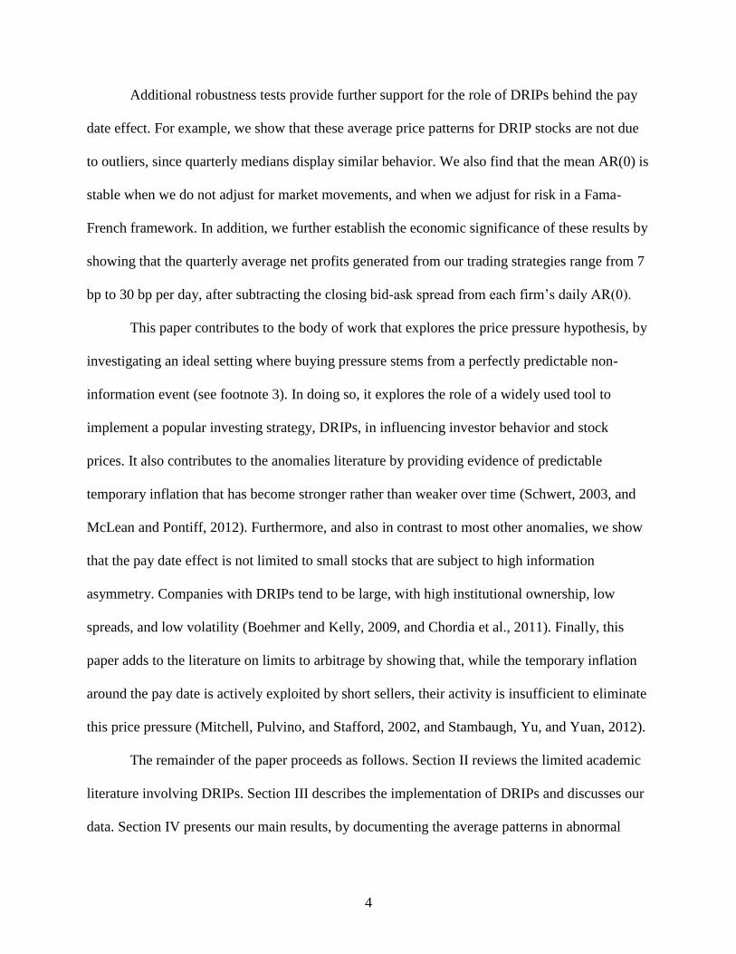
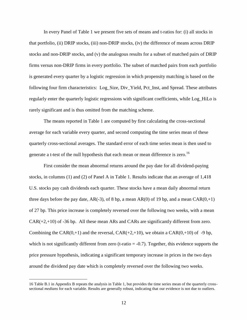
Figure 2 provides a first glance at our main results. Here we examine the price patterns

around the dividend pay date for two portfolios: all dividend-paying stocks, and a subset of high

dividend yield stocks that are hard to arbitrage.5 Panels A and B plot the abnormal returns (ARs)

and cumulative abnormal returns (CARs) for the subset of DRIP stocks in each portfolio, while

Panels C and D plot the analogous ARs and CARs for the subset of non-DRIP stocks.

Panel A of Figure 2 reveals that the abnormal returns for these two portfolios of DRIP

stocks are significantly positive on days -3, 0, and +1, and significantly negative on day +2 as

well as several subsequent days. In addition, these ARs are significantly larger in magnitude for

the second portfolio of high yield DRIP stocks that are hard to arbitrage. Panel B shows that the

highest CAR for each portfolio is attained on day +1, before reversing toward zero on subsequent

days. For the second portfolio, the mean AR(0) is 85 bp, and the CAR reaches a peak that

4 The three-day settlement period for U.S. stocks became effective with SEC Rule 15c6-1, in July 1995.

5 The second portfolio includes the subset of all dividend-paying stocks each quarter that are in the top 40% by

dividend yield, the bottom 40% by institutional ownership, and the top 40% by bid ask spread.

3

exceeds 1 percent on day +1. It is noteworthy that the series of negative ARs following day +1

accumulate to offset the entire price spike from this event. Thus the price reversal completely

offsets the temporary inflation around the pay date for these portfolios of DRIP stocks.

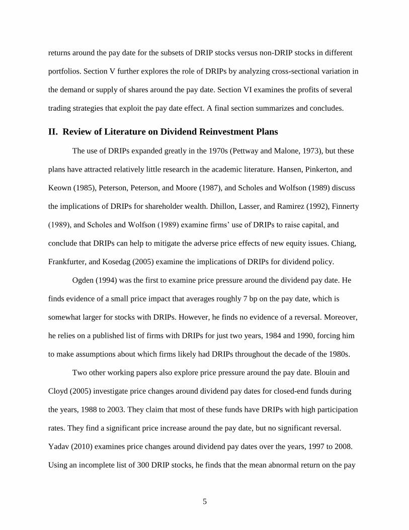
Panels C and D of Figure 2 reveal that the analogous portfolios of non-DRIP stocks also

display significant temporary inflation around the pay date. However, these ARs and CARs are

much smaller in magnitude. For example, for the second portfolio of high yield non-DRIP stocks

that are hard to arbitrage, the CAR reaches a maximum of just 37 bp on day +1.6

We further explore the role of company-sponsored DRIPs and confirm the findings above

by examining a matched sample of DRIP and non-DRIP stocks, and by using regression analysis.

We also investigate cross-sectional variation in the demand and supply of shares around the pay

date. This analysis shows that the pay date effect: (i) increases with greater demand due to

greater DRIP participation, and (ii) induces a greater supply of shares by attracting short sellers.

Finally, we examine the performance of several trading strategies that prescribe holding

certain portfolios of DRIP stocks on their respective pay dates (i.e., buy at the close on day -1

and sell at the close on day 0). Across all quarters in the sample period, 1996 - 2009, this strategy

generates a mean abnormal return of 31 bp per day for all DRIP stocks, 58 bp per day for DRIP

stocks with a high dividend yield, and 92 bp per day for high yield DRIP stocks that are hard to

arbitrage. The quarterly averages of these daily streams of abnormal profits (AR(0)) are positive

in at least 50 of the 56 quarters in our sample. In addition, they are significantly related to time

series movements in market sentiment, transaction costs, the dividend premium, and the VIX.7

6 One potential reason for this significant (albeit smaller) price spike for non-DRIP stocks is that retail brokerage

houses also offer their clients the opportunity to reinvest dividends automatically, even for stocks that have no

company-sponsored DRIP. In addition, some shareholders might reinvest their dividend income on their own. 7 To put the economic significance of these results in perspective, the performance of our second strategy (58 bp per

day) accumulates to 12% per month. In comparison, the momentum anomaly returns about 1% per month, and the

dividend premium anomaly returns 41 bp per month (Jegadeesh and Titman, 2001, Hartzmark and Solomon, 2013).

4

Additional robustness tests provide further support for the role of DRIPs behind the pay

date effect. For example, we show that these average price patterns for DRIP stocks are not due

to outliers, since quarterly medians display similar behavior. We also find that the mean AR(0) is

stable when we do not adjust for market movements, and when we adjust for risk in a Fama-

French framework. In addition, we further establish the economic significance of these results by

showing that the quarterly average net profits generated from our trading strategies range from 7

bp to 30 bp per day, after subtracting the closing bid-ask spread from each firm’s daily AR(0).

This paper contributes to the body of work that explores the price pressure hypothesis, by

investigating an ideal setting where buying pressure stems from a perfectly predictable non-

information event (see footnote 3). In doing so, it explores the role of a widely used tool to

implement a popular investing strategy, DRIPs, in influencing investor behavior and stock

prices. It also contributes to the anomalies literature by providing evidence of predictable

temporary inflation that has become stronger rather than weaker over time (Schwert, 2003, and

McLean and Pontiff, 2012). Furthermore, and also in contrast to most other anomalies, we show

that the pay date effect is not limited to small stocks that are subject to high information

asymmetry. Companies with DRIPs tend to be large, with high institutional ownership, low

spreads, and low volatility (Boehmer and Kelly, 2009, and Chordia et al., 2011). Finally, this

paper adds to the literature on limits to arbitrage by showing that, while the temporary inflation

around the pay date is actively exploited by short sellers, their activity is insufficient to eliminate

this price pressure (Mitchell, Pulvino, and Stafford, 2002, and Stambaugh, Yu, and Yuan, 2012).

The remainder of the paper proceeds as follows. Section II reviews the limited academic

literature involving DRIPs. Section III describes the implementation of DRIPs and discusses our

data. Section IV presents our main results, by documenting the average patterns in abnormal

5

returns around the pay date for the subsets of DRIP stocks versus non-DRIP stocks in different

portfolios. Section V further explores the role of DRIPs by analyzing cross-sectional variation in

the demand or supply of shares around the pay date. Section VI examines the profits of several

trading strategies that exploit the pay date effect. A final section summarizes and concludes.

II. Review of Literature on Dividend Reinvestment Plans

The use of DRIPs expanded greatly in the 1970s (Pettway and Malone, 1973), but these

plans have attracted relatively little research in the academic literature. Hansen, Pinkerton, and

Keown (1985), Peterson, Peterson, and Moore (1987), and Scholes and Wolfson (1989) discuss

the implications of DRIPs for shareholder wealth. Dhillon, Lasser, and Ramirez (1992), Finnerty

(1989), and Scholes and Wolfson (1989) examine firms’ use of DRIPs to raise capital, and

conclude that DRIPs can help to mitigate the adverse price effects of new equity issues. Chiang,

Frankfurter, and Kosedag (2005) examine the implications of DRIPs for dividend policy.

Ogden (1994) was the first to examine price pressure around the dividend pay date. He

finds evidence of a small price impact that averages roughly 7 bp on the pay date, which is

somewhat larger for stocks with DRIPs. However, he finds no evidence of a reversal. Moreover,

he relies on a published list of firms with DRIPs for just two years, 1984 and 1990, forcing him

to make assumptions about which firms likely had DRIPs throughout the decade of the 1980s.

Two other working papers also explore price pressure around the pay date. Blouin and

Cloyd (2005) investigate price changes around dividend pay dates for closed-end funds during

the years, 1988 to 2003. They claim that most of these funds have DRIPs with high participation

rates. They find a significant price increase around the pay date, but no significant reversal.

Yadav (2010) examines price changes around dividend pay dates over the years, 1997 to 2008.

Using an incomplete list of 300 DRIP stocks, he finds that the mean abnormal return on the pay

6

date is larger for his sample of DRIP stocks, compared to all stocks. In addition, similar to the

result in Panel D of Figure 2, he documents a significant abnormal return three days before the

pay date, and attributes this price spike to shareholders who buy more shares on day -3, and use

their dividend income to settle the trades three days later. He then focuses the remainder of his

paper on potential microstructure determinants of this price spike on day -3.

III. Transfer Agents, DRIP Participation, and the Data

III.A. Transfer Agents and the Administration of Company-Sponsored DRIPs,

Firms commonly enlist a transfer agent to manage the ownership record for all investors

who trade the company’s shares. Transfer agents ensure that all ownership rights are properly

allocated to the shareholders of record, including voting rights, the right to new shares issued

from stock splits, stock dividends or rights offerings, and the right to cash dividends. Firms also

typically rely on their transfer agent to administer company-sponsored DRIPs.

Details regarding the implementation of each company-sponsored DRIP vary across

firms, and are communicated to investors through a prospectus filed with the SEC, or a

document distributed by the firm or the transfer agent. Two transfer agents that manage a

substantial portion of all DRIPs sponsored by U.S. companies are Wells Fargo Shareowner

Services and Computershare Trust Company. These two transfer agents have made DRIP

documents available on their own web sites for a sizable number of their affiliated companies.8

This DRIP documentation typically describes three important features about the purchase

of shares involved in the DRIP: (i) how the shares are to be purchased, (ii) when the shares are to

be purchased, and (iii) what purchase price is to be charged to DRIP participants. First, each

quarter the company will direct the transfer agent to either purchase newly issued shares from the

8 The web site of Computershare is https://www-us.computershare.com/investor/plans/planslist.asp?stype=drip, and

the web site for Wells Fargo is https://www.shareowneronline.com/UserManagement/DisplayCompany.aspx.

7

company, or purchase existing shares in the open market. Second, if the transfer agent is told to

purchase shares in the open market, it is typically directed to purchase the shares “as soon as

possible after receiving the funds.” This common wording implies a fairly strong incentive for

transfer agents to purchase shares in the open market on the dividend pay date (as soon as the

dividend funds are received), in order to avoid litigation regarding any potential breach of

fiduciary duty. Third, the price applied to every DRIP participant is typically the trade-weighted

average price that applies to all shares bought to satisfy the DRIP if shares are purchased on the

open market, or the closing price on the pay date if newly issued shares are purchased from the

company. Appendix A provides excerpts from the DRIP documents for two firms. These

documents describe the responsibilities of the transfer agent, and demonstrate the relevant details

common in these plans

III.B. DRIP Participation and the Number of Shareholders of Record

We conjecture that the existence and implementation of company-sponsored DRIPs is a

major force behind the pay date effect documented in this study. In designing tests of this

conjecture, we are limited by the fact that no firm-specific data are available on the participation

rates in company-sponsored DRIPs, or the shareholdings of DRIP participants.9 Given this

limitation, we test this conjecture several ways in our main analysis, by separately examining the

divergent behavior of firms with and without company-sponsored DRIPs. In addition, in our

extended analysis of the role of DRIPs, we develop a firm-specific proxy for DRIP participation

rates based on the number of shareholders of record for a firm. This proxy is motivated below.

9 We have had many conversations with companies, transfer agents, and retail brokerage houses to request data on

firm-specific DRIP participation rates, the shareholdings of DRIP participants, and the timing and pricing of

purchases made in the implementation of DRIPs. None of the entities we communicated with were willing to share

any data or discuss their implementation of DRIPs, with many expressing a concern about the risk of litigation.

8

The shares of firms with no company-sponsored DRIP are normally held in “street name”

in retail brokerage accounts. This means that the shares are registered in the name of the

brokerage firm through which the stock is bought, rather than the investor who purchased the

stock. In this case, all communication between the company and the investor is routed through

the broker. This practice gives the brokerage house control over details involving shareholder

rights for their retail customers, and reduces the cost of providing brokerage services. The typical

brokerage house charges a substantial fee to retail clients who ask to become shareholders of

record, in order to discourage such requests. Thus, a few retail brokerage houses commonly

operate as the shareholders of record on behalf of their numerous investors in non-DRIP stocks.

In contrast, firms with company-sponsored DRIPs routinely require an individual

investor to become the shareholder of record in order to participate in their DRIP. This

requirement helps to grow and stabilize retail ownership, and results in all communication being

made directly between the firm and its shareholders. It also enables the firm’s transfer agent to

administer the DRIP directly to the firm’s shareholders.

As a result of this struggle between firms and retail brokerage houses to control the

record of ownership, the official number of shareholders (Compustat annual variable, CSHR)

drastically understates the true number of investors for the typical firm. However, we find that

the average number of shareholders is significantly larger for firms with company-sponsored

DRIPs than for firms without DRIPs. This difference presumably reflects participation in DRIPs.

Furthermore, we argue that cross-sectional variation in the number of shareholders across DRIP

firms reveals information about firm-specific DRIP participation rates. We exploit this feature of

DRIPs to generate a proxy for DRIP participation based on the actual number of shareholders at

a firm, relative to the number expected (predicted) at other DRIP firms with similar attributes.

9

III.C. Data and Variables

We use daily returns for all NYSE, AMEX, and NASDAQ common stocks (CRSP share

code 10 or 11) during the period, July 1975 through December 2009. We analyze benchmark-

adjusted abnormal returns to measure stock price performance (see Daniel, Grinblatt, Titman,

and Wermers, 1997). The abnormal return is defined as the difference between the actual return

on a stock and the return on an equally weighted portfolio of all firms in the same size and book-

to-market quintiles. For each stock, we obtain annual portfolio assignments into size and book-

to-market quintiles from Russ Wermers’s website.10

We obtain the pay dates of all quarterly cash dividend distributions from CRSP (distcd =

1200 - 1299). If a pay date is on a weekend, we recognize that the dividend payment will occur

on the next business day. We keep all quarterly dividend events for which: (a) the number of

days between the ex-dividend day and the pay date is at least 10 and no more than 45; (b) the

number of days between the ex-dividend day and the record date is at least 2 and no more than 7;

and (c) there are at least 20 days between a firm’s consecutive dividend pay dates. These screens

help to ensure that we ignore events with coding errors, and reduce the impact of ex-dividend

price effects on the pay date price effect.11

For the years, 1996 - 2002, we have also obtained annual lists of firms with company-

sponsored DRIPs from the American Association of Individual Investors (AAII) annual

publications on firms with DRIPs. For the subsequent years, 2003 - 2009, we obtained quarterly

lists of DRIP firms using the AAII Stock Investor Pro web site. The AAII annual publications for

the earlier years, 1996 - 2002, also provide information about certain features of these DRIPs.

For example, for this sub-period, 25% of all DRIPs charged a fee for participation, while 7%

10 Portfolio assignments for NYSE, AMEX, and NASDAQ stocks from CRSP are available since 1975, based on

the approach in Wermers (2003), at http://www.smith.umd.edu/faculty/rwermers/ftpsite/Dgtw/coverpage.htm.

11 These screens eliminate 11,729 quarterly dividend payments out of the 299,813 events in the sample since 1975.

10

offered the opportunity to reinvest dividends at a discount of 1% to 5% below the market price.12

We analyze the following dependent variables, which represent abnormal returns

measured over six different portions of the 21-day event window, (-10,+10), covering the two

weeks before and after the pay date. The timing of these six measures is dictated by the evidence

in Figure 2, which indicates significant positive abnormal returns on days -3, 0, and +1, which

are followed by a series of smaller but significant negative abnormal returns in the ensuing days.

Dependent variables:

1) AR(-3) = abnormal return on day -3, three days before the pay date;

2) AR(0) = abnormal return on the dividend pay date;

3) CAR(0,+1) = cumulative abnormal return over days 0 and +1;

4) CAR(+2,+5) = cumulative abnormal return over days +2 through +5;

5) CAR(+2,+10) = cumulative abnormal return over days +2 through +10;

6) CAR(0,+10) = cumulative abnormal return over days 0 through +10;

where AR(t) = abnormal benchmark-adjusted return for the stock on day t relative to the

dividend pay date (i.e., day 0), using the equally weighted benchmark return based on firms

in the same size and book-to-market quintiles.

Explanatory variables:

1) DRIP = 1 if the firm has a company-sponsored DRIP, or 0 otherwise;

2) Size = the firm’s daily market capitalization averaged over days -10 through -6,

where daily market capitalization is taken from CRSP;

3) Div_Yield = the firm’s percentage dividend yield, computed as the cash dividend amount

from CRSP divided by the firm’s daily closing stock price, multiplied by 100,

and averaged over days -10 through -6;

4) Pct_INST = the percentage of total shares outstanding owned by institutional investors for

the quarter, taken from 13F filings;

5) Spread = the daily closing bid-ask spread, as a percentage of the daily closing price,

taken from CRSP, and averaged over days -10 through -6;13

12 In analysis not reported here, we find no evidence that the existence or magnitude of a fee or a discount affects

the pay date effect, for the 25% of DRIP firms that charge a fee, or the 7% of DRIP firms that offer a discount.

13 Chung and Zhang (2013) show that the CRSP-based spread is highly correlated with the TAQ-based spread

across stocks, using data from 1993 through 2009. Their results indicate that the simple CRSP-based spread can

effectively be used in lieu of the TAQ-based spread in academic research that focuses on cross-sectional analysis.

11

6) Log_HiLo = the intraday percentage stock return volatility, measured as the natural log of

the ratio of the daily high and low prices multiplied by 100, taken from CRSP,

and averaged over days -10 through -6;

7) CSHR = the (annual) number of shareholders of record, taken from Compustat;

8) Firm_Age = the number of quarters since the firm first appeared on CRSP.

The relevant explanatory variables are known at least one week prior to the pay date. Thus, the

results in this paper lead to predictive trading strategies that can easily be implemented.14

We examine three portfolios of stocks each quarter that vary in terms of dividend yield

and the limits to arbitrage that they face. These portfolios are generated by first independently

sorting all dividend-paying stocks each quarter according to their: (i) dividend yield, (ii)

institutional ownership, and (iii) bid-ask spread. Then we construct portfolios I - III, as follows:

I (All Stocks): All dividend-paying stocks each quarter;

II (High_DY): Top 40% of dividend-paying stocks each quarter by dividend yield;

III (Hard_Arb): Top 40% of dividend-paying stocks each quarter by dividend yield,

bottom 40% by institutional ownership, and top 40% by spread.15

IV. Main Results: The Pay Date Effect

IV.A. The Average Pay Date Effect and Firm Characteristics for Portfolios I - III

Table 1 provides the mean abnormal returns for different time frames around the

dividend pay date for portfolios I - III, as well as descriptive statistics for the average firm

characteristics in these portfolios. Each panel presents results for a different portfolio of stocks,

with and without DRIPs. Panel A gives the results for all Stocks (I), while Panels B and C

provide the analogous results for the High_DY portfolio (II) and the Hard_Arb portfolio (III).

14 Computing the average daily values of Size, Div_Yield, Spread, and Log_HiLo over days -10 through -6 ensures

that we measure these firm attributes close to the dividend pay date (on day 0). We have also analyzed these firm

attributes over different time frames before or after the event window, with similar results.

15 Other studies that use institutional ownership or transaction costs to examine the influence of limits to arbitrage

on stock return performance include Asquith et al. (2005), Berkman et al. (2009), Berkman et al. (2012), Boehme et

al. (2006), Diether et al. (2002), Nagel (2005), and Sadka and Scherbina (2007).

12

In every Panel of Table 1 we present five sets of means and t-ratios for: (i) all stocks in

that portfolio, (ii) DRIP stocks, (iii) non-DRIP stocks, (iv) the difference of means across DRIP

stocks and non-DRIP stocks, and (v) the analogous results for a subset of matched pairs of DRIP

firms versus non-DRIP firms in every portfolio. The subset of matched pairs from each portfolio

is generated every quarter by a logistic regression in which propensity matching is based on the

following four firm characteristics: Log_Size, Div_Yield, Pct_Inst, and Spread. These attributes

regularly enter the quarterly logistic regressions with significant coefficients, while Log_HiLo is

rarely significant and is thus omitted from the matching scheme.

The means reported in Table 1 are computed by first calculating the cross-sectional

average for each variable every quarter, and second computing the time series mean of these

quarterly cross-sectional averages. The standard error of each time series mean is then used to

generate a t-test of the null hypothesis that each mean or mean difference is zero.16

First consider the mean abnormal returns around the pay date for all dividend-paying

stocks, in columns (1) and (2) of Panel A in Table 1. Results indicate that an average of 1,418

U.S. stocks pay cash dividends each quarter. These stocks have a mean daily abnormal return

three days before the pay date, AR(-3), of 8 bp, a mean AR(0) of 19 bp, and a mean CAR(0,+1)

of 27 bp. This price increase is completely reversed over the following two weeks, with a mean

CAR(+2,+10) of -36 bp. All these mean ARs and CARs are significantly different from zero.

Combining the CAR(0,+1) and the reversal, CAR(+2,+10), we obtain a CAR(0,+10) of -9 bp,

which is not significantly different from zero (t-ratio = -0.7). Together, this evidence supports the

price pressure hypothesis, indicating a significant temporary increase in prices in the two days

around the dividend pay date which is completely reversed over the following two weeks.

16 Table B.1 in Appendix B repeats the analysis in Table 1, but provides the time series mean of the quarterly cross-

sectional medians for each variable. Results are generally robust, indicating that our evidence is not due to outliers.

13

The remaining columns of Panel A in Table 1 compare the behavior of all DRIP stocks

versus all non-DRIP stocks. This comparison indicates that the temporary price pressure on the

pay date is significantly larger in magnitude for firms with DRIPs (see AR(0) in columns 3

through 7)). The additional rows in Panel A reveal that the average DRIP firm is significantly

larger in size, and tends to have a larger dividend yield, greater institutional ownership, smaller

spreads, lower stock return volatility, a larger number of shareholders, and greater firm age.

The matched pairs reported in column (8) and (9) control for these differences in firm

characteristics. As a result, column (10) indicates that the mean differences in dividend yield and

spread are no longer significant across matched pairs. On the other hand, the mean differences in

institutional ownership and size remain significantly different from zero, although small in

magnitude. We also find that the matched set of DRIP stocks have a mean AR(0) of 31 bp, which

is significantly larger than the mean AR(0) of 12 bp for the matched set of non-DRIP stocks. In

addition, consistent with our earlier discussion, the mean (median) number of shareholders

(CSHR) is significantly larger for DRIP stocks than for non-DRIP stocks. For the matched

sample, the median DRIP firm has 6,863 shareholders and the median non-DRIP firm has 2,619

shareholders. Finally DRIP stocks tend to be older than the matched non-DRIP stocks.

Panels B and C of Table 1 give analogous results for the successively smaller portfolios

with a higher dividend yield (II) and greater limits to arbitrage (III). As we proceed to Panels B

and C, the price run-up and reversal around the pay date grow larger in magnitude, and their

mean differences across DRIP versus non-DRIP stocks become larger and more significant. The

other relative attributes of DRIP firms versus non-DRIP firms from Panel A are fairly stable

across the successive portfolios. It is noteworthy that, in contrast to many other anomalies, this

pay date effect is not limited to small stocks that are subject to high information asymmetry. In

14

each panel of Table 1, the subset of DRIP firms in each portfolio tend to be larger and older, with

more shareholders, higher institutional ownership, smaller spreads, and lower volatility.

We again note that non-DRIP firms also display significant, albeit smaller, temporary

price pressure around the pay date. This result may be due to shareholders who reinvest their

dividend income on their own, or through participation in DRIPs offered by brokerage houses

that also offer DRIPs to their retail clients, even for firms with no company-sponsored DRIP.

In every Panel of Table 1, we also present the mean abnormal return on the ex-dividend

date, along with the mean difference between the abnormal return on the pay date versus that on

the ex-date.17

For each subset of DRIP stocks in Panels A - C, the mean AR(0) on the pay date is

significantly larger than the mean abnormal return on the ex-date. In contrast, for each subset of

non-DRIP stocks, the mean AR(0) on the pay date is significantly smaller than that on the ex-

date. We also note that the mean abnormal return on the ex-date for DRIP stocks tends to be

smaller than that for non-DRIP stocks (see column 7 in Table 1). This evidence indicates that the

dividend pay date receives greater price pressure for DRIP stocks, while the ex-date is subject to

greater price pressure for non-DRIP stocks. However, this difference seems to be partially

associated with different firm characteristics across the two subsamples, since it diminishes for

our pairs of firms matched by firm characteristics (see column 10). Together, these results

reinforce the importance of DRIPs as a major force behind the dividend pay date effect.

IV.B. Correlations across Abnormal Returns around the Pay Date for Portfolios I - III

Table 2 presents the average correlations across the abnormal return measures around the

pay date (AR(-3), AR(0), and CAR(0,+1)) and the measures of subsequent reversal (CAR(+2,+5)

and CAR(+2,+10)). Similar to Table 1, each quarter we first compute every pairwise correlation

17 Hartzmark and Solomon (2013) provide evidence of temporary price pressure during the month that dividends

are expected, which is followed by a reversal in the following month. They focus on the abnormal returns around the

ex-dividend date, and do not consider the pay date effect or the impact of DRIPs on their results.

15

across all stocks in each portfolio, I - III, as well as across the subsets of DRIP stocks or non-

DRIP stocks in each portfolio. We then calculate the time series mean of every pairwise

correlation across all quarters, and present the results in Panels A - C for portfolios I - III,

respectively. The standard error of the time series mean is again used to test the null hypothesis

that every mean correlation is zero. Pearson correlations are presented above the diagonal and

Spearman correlations appear below the diagonal.

First consider the correlations involving AR(-3). Table 2 reveals only weak evidence that

AR(-3) is correlated with the price spike around the pay date (AR(0) or CAR(0,+1)), or the

subsequent reversal (CAR(+2,+5) or CAR(+2,+10)) for any portfolio. In addition, there is no

tendency for the correlations involving AR(-3) to be larger for DRIP stocks compared with non-

DRIP stocks. This outcome is not surprising since the explanation for this price spike proposed

by Ogden (1994) and Yadav (2010), involving a 3-day settlement for buying additional shares,

applies to shareholders of both DRIP stocks and non-DRIP stocks.

Next consider the correlations between the relative magnitudes of the price inflation

around the pay date (AR(0) or CAR(0,+1)) and the subsequent reversal (CAR(+2,+5 or

CAR(+2,+10)), highlighted in the shaded areas of Table 2. These results indicate that the

abnormal returns around the pay date are significantly negatively correlated with the cumulative

abnormal returns over the following two weeks, for each portfolio. Furthermore, the magnitude

of these negative correlations increases as we consider the progressively finer subsets of stocks

with a higher dividend yield and greater limits to arbitrage, in the successive portfolios I - III.

These results reinforce our evidence in Table 1, to provide further support for a systematic

tendency for stock prices to increase around the pay date and reverse over the following two

weeks, consistent with the temporary price pressure hypothesis.

16

V. Further Exploration of the Role of DRIPs behind the Pay Date Effect

This section examines the association between the demand or supply of shares and the

pay date effect. First we analyze how cross-sectional variation in demand may influence the

magnitude of this temporary price pressure, by constructing a firm-specific proxy for DRIP

participation rates and relating this proxy to AR(0) and CAR(0,+1). Second, we investigate how

the pay date effect influences the supply of shares by attracting short sellers around the pay date.

V.A. Demand for Shares, DRIP Participation, and the Pay Date Effect

In this section we first propose a firm-specific proxy for DRIP participation rates based

on the firm’s number of shareholders. We then examine whether firms with greater demand for

shares around the pay date, through greater DRIP participation, tend to have a larger pay date

effect (AR(0) and CAR(0,+1)). We begin by specifying the following model that describes the

relation between the number of shareholders of record for a firm and certain firm characteristics:

Log_CSHRin = α0 + α1 Firm_Agein + α2 Log_Sizein + α3 Div_Yieldin

+ α4 Pct_Instin + α5 Spreadin + α6 Log_Hiloin + εin . (1)

This specification follows the convention in previous efforts to model determinants of CSHR,

which take the natural log of both CSHR and firm size in order to mitigate the positive skewness

inherent in these two variables.18

We estimate Equation (1) for the cross-section of either DRIP firms or non-DRIP firms

each quarter. This approach enables our proxy to reflect how DRIP participation rates vary, not

only in the cross-section, but also across quarters. The left two columns in Table 3 present the

Fama-MacBeth mean coefficients for this model, applied each quarter to the subsets of all DRIP

18 For example, see Grullon, Kanatas, and Weston (2004) and Larkin, Leary, and Michaely (2013).

17

stocks and all non-DRIP stocks, separately. The third column presents the differences in the

respective mean coefficients across DRIP firms versus non-DRIP firms.

For both subsets of DRIP stocks and non-DRIP stocks, the mean coefficients in the first

two columns of Table 3 indicate a significantly larger number of shareholders for a firm with

greater age, larger size, higher dividend yield, lower institutional ownership, a higher spread, and

greater volatility. Furthermore, the third column indicates that the impact of firm age on the

number of shareholders is significantly smaller for DRIP firms relative to non-DRIP firms. In

contrast, the third column also reveals that the mean coefficients for firm size, dividend yield,

and institutional ownership are significantly larger in magnitude for the subset of DRIP firms.19

We use the actual and fitted values from Equation (1) each quarter, to construct our proxy

for firm-specific DRIP participation rates, as follows:

DRIP_Partin = (Actual Value of Log_CSHRin / Fitted Value of Log_CSHRin).

This proxy is generated separately for the subsets of firms with and without DRIPs each quarter.

It captures the actual number of shareholders for each DRIP (or non-DRIP) firm, relative to the

number expected at other DRIP (or non-DRIP) firms with similar attributes.

We argue that this proxy contains relevant information about DRIP participation rates for

the subset of DRIP firms, while it should be uninformative for the subset of non-DRIP firms.

That is, when the number of shareholders (Log_CSHR) at a DRIP firm exceeds (or falls short of)

that predicted by Equation (1) for other DRIP firms with similar characteristics, this excess (or

shortfall) is likely to reflect greater (or lower) participation in the firm’s DRIP. In contrast, this

proxy should be meaningless for non-DRIP firms in terms of its relation to the pay date effect.

19 The Chow Test at the bottom of the third column in Table 3 verifies that the set of all coefficients from a panel

regression for Equation (1) is significantly different for DRIP stocks versus non-DRIP stocks.

18

Ceterus paribus, we expect that a higher participation rate in a firm’s DRIP reflects

greater demand for shares, and should thus be associated with a larger pay date effect. We test

this prediction by specifying a model that includes DRIP_Partin and other firm characteristics

from Equation (1) as potential determinants of abnormal returns around the pay date, as follows:

[AR(0)in or CAR(0,+1)in] = β0 + β1 DRIP_Partin + β2 Log_Sizein + β3 Div_Yieldin

+ β4 Pct_Instin + β5 Spreadin + β6 Log_HiLoin + υin. (2)

Once again, we expect a positive coefficient for DRIP_Part (β1) when Equation (2) is estimated

for the set of DRIP firms, while β1 should be zero for the set of non-DRIP firms.

The remaining columns in Table 3 present the results. We now estimate the panel in

Equation (2) with standard errors clustered on the firm and the quarter of the dividend payment,

applied separately to all DRIP stocks or all non-DRIP stocks. Results indicate that, for the subset

of DRIP firms, a larger price spike on day 0 (or days 0 and +1) is significantly associated with a

greater DRIP participation rate, as well as with lower institutional ownership or a larger dividend

yield, spread, or volatility. In contrast, for non-DRIP firms, this DRIP participation proxy has no

association with AR(0) or CAR(0,+1), as expected. Furthermore, the coefficient of DRIP_Partin

is significantly larger in magnitude for the subset of DRIP firms, relative to non-DRIP firms, as

are the coefficients on two other firm characteristics in each set of results presented in Table 3.20

V.B. Supply of Shares: Short Selling around the Pay Date

If sophisticated investors try to exploit the temporary price increase around the pay date,

then we would expect the volume of short selling to increase at the time of the largest positive

price spikes, on days -3 and 0. We investigate this possibility by examining daily movements in

abnormal short volume (ASV) over the event window (-10,+10). This variable is constructed

20 Once again, the Chow Test in column (3) verifies that the set of all coefficients from Equation (2) is significantly

different across the subsets of DRIP stocks versus non-DRIP stocks.

19

from Reg SHO data on daily short volume over the ten quarters covering the period, January

2005 through June 2007, as follows:

ASVitn = (SV / TV)itn - Normal(SV / TV)in ,

where (SV / TV)itn = short volume as proportion of total volume for stock i on day t in quarter n;

and Normal(SV / TV)in = the mean of (SV / TV)itn over days +11 through +30, after day 0.21

We then examine the mean values of ASVitn for all 21 days in the event window, t =

(-10,+10), for the subsets of DRIP stocks versus non-DRIP stocks in the portfolio of all

dividend-paying stocks (I), and the portfolio of stocks with a high dividend yield (II). For a firm

event to be included in this analysis, we require at least one day with non-zero shorting volume

in the window (+11, +30). This requirement reduces the sample to 6,451 events for portfolio I,

and 2,261 events for portfolio II.22

As before, for every quarter we first compute the cross-sectional average of ASV(t) for

each day, and then calculate the time series mean of these cross-sectional averages over the 10

quarters in the sample period for which we have short sales data. Likewise, the confidence

intervals for the ASV(t) are obtained from the standard errors of the time series means, for the

subset of DRIP stocks or non-DRIP stocks in portfolio II, for all 21 days in the event window.23

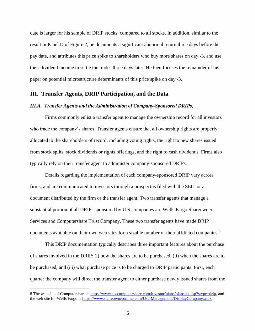
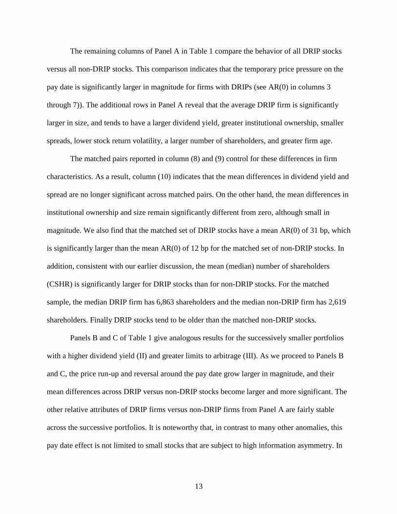
Results are plotted in Panels A and B of Figure 3 for the subsets of DRIP stocks and non-

DRIP stocks, respectively, in portfolios I and II. For the two portfolios of DRIP stocks in Panel

A, average abnormal short volume is positive on all but one day in the event window, and it is

significantly greater than zero on days -3 and 0. In addition, the magnitude of the spikes in

21 Our daily short-sales data are obtained from the self-regulatory organizations (SROs) that made tick data on short

sales publicly available starting on January 2, 2005, as a result of the SEC’s Regulation SHO. Short sales data for

the NYSE are available through the TAQ database, and all other SROs make short sales data available on their

websites. The end date for the regulation SHO data in our sample is July 1, 2007. 22 We do not present the results for the third portfolio of high yield stocks that are hard to arbitrage (III), because of

small sample sizes (there are less than 10 events per quarter for the DRIP and non-DRIP subsets of this portfolio). 23 Similar to Figures 1 and 2, in Figure 3 the 95% confidence interval for portfolio II is conservative for portfolio I.

20

abnormal short volume on these two days increases somewhat as we move from the portfolio of

all DRIP stocks (I) to the subset of high yield DRIP stocks (II). For portfolio II, the average

abnormal short volume is 0.5% of total volume on day -3, and 1% of total volume on day 0.

For the analogous subsets of non-DRIP stocks analyzed in Panel B of Figure 3, we find

no evidence of abnormal short selling around the pay date. The average abnormal short volume

is small in magnitude for each day, and is never significantly greater than zero. This result is

consistent with the lower temporary price inflation for these subsets of non-DRIP stocks

documented in Figure 2 and Table 1. This evidence supports the view that short sellers try to

exploit the predictable price spikes around the pay date for DRIP stocks, but their activity is

insufficient to eliminate this temporary inflation.

VI. Strategies that Trade on this Price Pattern

VI.A. Quarterly Performance from Three Trading Strategies

In this section we analyze the performance of three alternative trading strategies that

attempt to profit from the price spike on day 0. These strategies prescribe holding the subsets of

DRIP stocks in each of our three portfolios, I - III, on their respective dividend pay dates. To

implement each strategy, for every day in our sample, we first identify every DRIP stock in each

portfolio that pays a dividend on the next day (t). Then we prescribe buying the subset of all such

DRIP stocks in each portfolio that pay dividends on the next day, and holding for 24 hours (i.e.,

buy at the close on day t-1 and sell at the close on day t). In addition, we assume a short position

on an equivalent amount of the S&P 500 index. This strategy earns the market-adjusted

abnormal return, AR(0)it, for each DRIP stock that pays a dividend on any given day t.24

24 Analysis of benchmark-adjusted abnormal returns yields similar results. In Appendix C we show that, for the two

portfolios that are most interesting from a trading perspective (II. High_DY and III. Hard_Arb), the average price

increase occurs gradually throughout the trading hours on day 0. Thus, buying at the close on day -1 and selling at

the close on day 0 captures the average AR(0). We have also analyzed two alternative strategies: (i) to hold each

21

For every day (t) in our sample period, we then compute the average across the AR(0)it

for all DRIP stocks in each portfolio (I - III) that pay dividends on that given date. The resulting

mean values, AR(0)t, reflect a daily time series of one-day average abnormal “profits” for each

strategy, for all days where at least one DRIP stock in each portfolio pays a dividend. Then, for

every quarter (n), we average these one-day mean abnormal returns, AR(0)t, across all days in

the quarter where at least one DRIP stock pays a dividend. The results reflect a quarterly time

series of average one-day abnormal returns, AR(0)n, from these three trading strategies. We then

track this quarterly average AR(0)n for each subset of DRIP stocks from portfolios I - III,

throughout all quarters of the sample period, 1996 to 2009.

VI.B. Time Series Movements in Quarterly Abnormal Profits

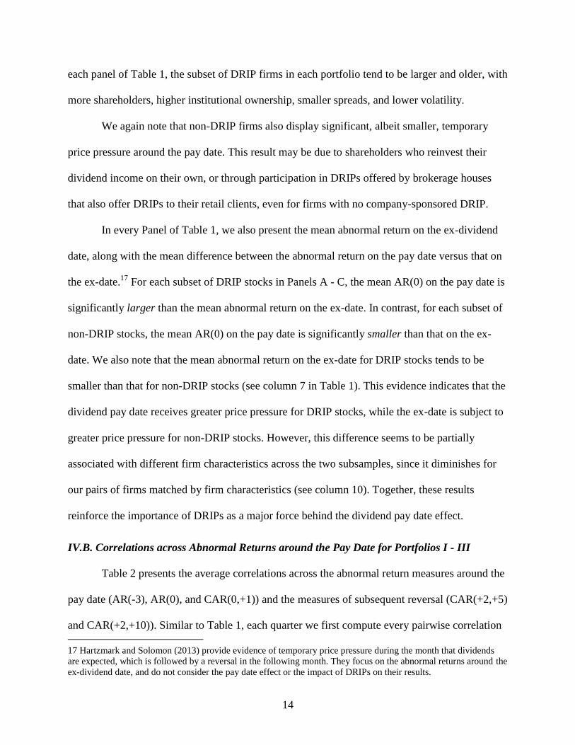
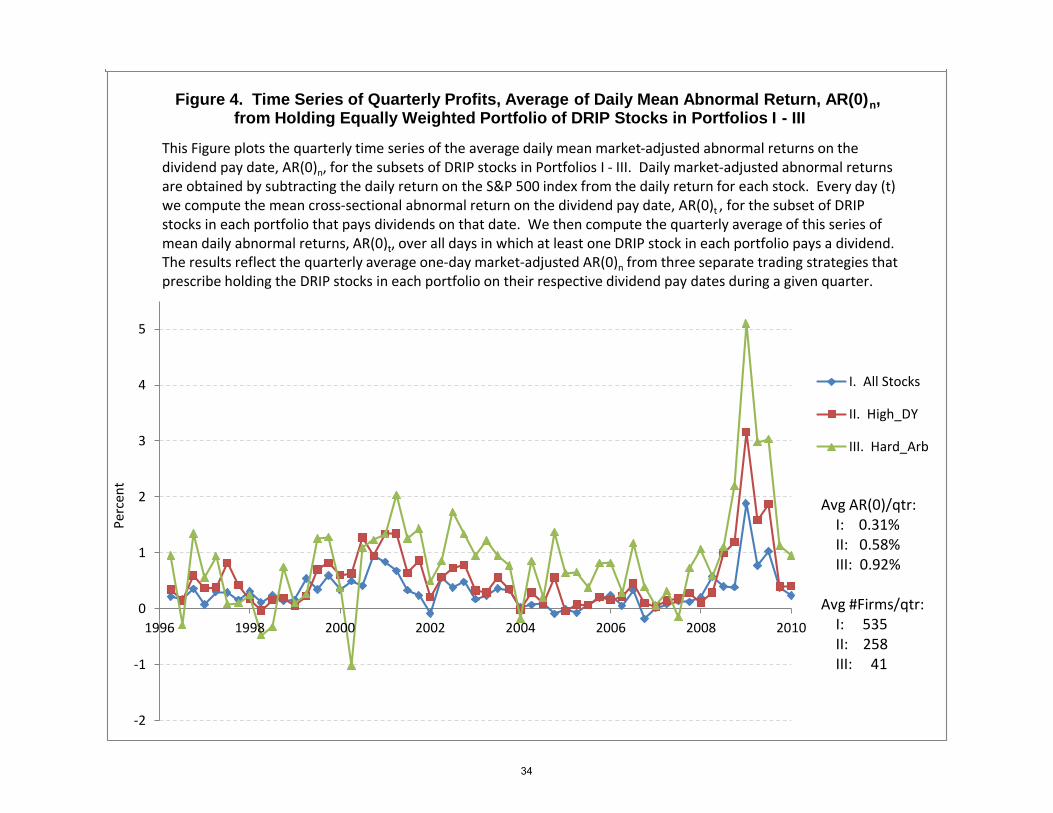
Figure 4 presents a time series plot of the quarterly mean one-day abnormal returns on the pay

date, AR(0)n, from applying these three trading strategies. For the portfolio of all dividend-

paying DRIP stocks (I), the mean quarterly values of AR(0)n are positive for 53 of the 56

quarters in the sample period, and the average one-day AR(0)n across all quarters is 0.31%. The

portfolio of high dividend yield stocks (II) yields a similar stream of quarterly average profits

that are positive for 53 quarters, and it generates a larger mean one-day AR(0)n of 0.58%.

Finally, the average one-day profit stream from stocks that are hard to arbitrage (III) is somewhat

more volatile, yet these profits are still positive in 50 quarters. This profit stream also generates a

higher mean one-day AR(0)n of 0.92% across all quarters in the sample.

Economic theory suggests that the magnitude of the quarterly average one-day AR(0)n

from these trading strategies should be larger following periods when there is greater investor

demand for dividend-paying stocks, or greater limits to arbitrage associated with the stocks held

portfolio of DRIP stocks on days 0 and +1, earning CAR(0,+1), and (ii) to be long these stocks on days 0 and +1,

and then short over days +2 - +5, earning CAR(0,+1) - CAR(+2,+5). This analysis yields similar conclusions.

22

in each strategy. This observation motivates the following regression model that specifies several

potential determinants of the quarterly time series of average one-day profits for each strategy:

AR(0)n = β0 + β1 Sentimentn-1 + β2 Spreadn-1 + β3 pdndn-1 + β4 VIXn-1 + εn , (3)

where AR(0)n = quarterly average of the time series of mean one-day profits, AR(0)t, for the

portfolio of DRIP stocks from each strategy, across all days in quarter n;

Sentimentn-1 = Baker and Wurgler (2006) sentiment index in quarter n-1;25

Spreadn-1 = mean daily closing percentage spread for the DRIP stocks in the portfolio of

high dividend yield stocks, across all days in quarter n-1;26

pdndn-1 = value-weighted dividend premium in quarter n-1 (Baker and Wurgler, 2004);

VIXn-1 = CBOE Volatility Index, averaged across the 3 months in quarter n-1.

First, the sentiment index of Baker and Wurgler is intended to capture the willingness of

investors to trade at prices not justified by fundamentals. We expect that periods with relatively

high market sentiment are likely to be followed by relatively high dividend reinvestment, and

thus high price pressure on the pay date. Second, a larger average spread represents a limit to

arbitrage that should reduce the willingness of arbitrageurs to trade against the pay date effect.

Third, changes over time in the dividend premium reflect changing demand for dividend-paying

stocks (Baker and Wurgler, 2004). We thus expect that periods with a stronger preference for

dividend paying stocks are followed by a larger pay date effect. Finally, the VIX measures

expectations about overall market volatility, so a larger VIX serves as a negative sentiment

indicator that may be followed by less demand for these stocks, and thus a lower mean AR(0).27

Table 4 provides regression results for the DRIP stocks in portfolios I - III, respectively.

First, the quarterly mean AR(0)n for each strategy is positively related to time series movements

in market sentiment during the previous quarter, and significantly so for portfolios II and III.

25 Monthly data on the sentiment index of Baker and Wurgler (2006) are available on Jeff Wurgler’s web site, along

with the components of their index, such as pdnd. We aggregate these monthly data to form quarterly figures.

26 The daily percentage Spread = (Ask - Bid)/((Ask + Bid)/2), where the closing Bid and Ask are taken from CRSP.

27 For further discussion of these issues involving limits to arbitrage and market sentiment, see Baker and Wurgler

(2006, 2007), Kumar and Lee (2006), Sadka and Scherbina (2007), and Schleifer and Vishny (1997).

23

Second, these profits have a significant positive association with transaction costs in the previous

quarter, across all three strategies. Third, the AR(0)n is significantly influenced by the dividend

premium in the previous quarter for the DRIP stocks in portfolio III. Finally, we find a negative

association between the profitability of our strategies and the VIX from the previous quarter,

which is significant for the DRIP stocks in portfolio III. We conclude from this analysis that,

consistent with economic theory, time-variation in the magnitude of price pressure around the

dividend pay date is significantly related to market sentiment, as well as limits to arbitrage.

VI.C. Extended Tests on the Time Series of Profits

Appendix D provides additional robustness tests to explore alternative possible

explanations for our results, and to examine the sensitivity of these results to additional analyses.

VI.C.1. Time Series Movements in Quarterly Actual Profits

One conspicuous feature of Figure 4 is the large spike in the mean one-day AR(0)n during

the last quarter of 2008, which ranges from 2% to 5% for these three strategies. In Figure D.1 we

explore the possibility that this spike in market-adjusted abnormal returns is due to the large

market decline during the financial crisis. We thus plot the analogous time series of quarterly

actual profits from these three strategies (Return(0)n), without subtracting the market return.

As expected, the mean one-day actual Return(0)n in the last quarter of 2008 is smaller in

Figure D.1 than it is in Figure 5; it now ranges from 0% to 3.5% for portfolios I - III, when we

do not short the (negative) market return during this quarter. On the other hand, a substantial

spike in actual performance remains during this quarter in Figure D.1, especially for the DRIP

stocks in portfolio III. Furthermore, the mean actual returns in Figure D.1 tend to be slightly

higher than the analogous abnormal returns in Figure 5, for most quarters throughout the sample

period, when we do not subtract the market return that is positive in most quarters. As a result,

24

the average one-day actual return (Returna(0)n) across all quarters is similar to the average one-

day abnormal return (AR(0)n) presented in Figure 4, for all three strategies.

VI.C.2. Quarterly Net Profits after Deducting Assumed Transaction Costs in the Bid-Ask Spread

Our trading strategies allow the use of market-on-close orders, which would yield the

mean close-to-close performance measures, Return(0)n or AR(0)n, documented in this study. This

means that there is no need to consider the spread as a transaction cost. Still, in Figure D.2 we

examine the analogous time series of quarterly net profits for each strategy, Return(0)n - TC, as if

all purchases and sales took place at the daily close and incurred the closing spread.

Panels A - C of Figure D.2 track the actual and net profits from each strategy in turn.

Each Panel reveals that, following decimalization in the second quarter of 2002, spreads decline

so that this stream of net profits (Return(0)n - TC) tracks the actual profits (Return(0)n) closely,

especially for portfolios I and II. Across all quarters since decimalization, the average one-day

net returns are positive for all three strategies, even after deducting these assumed transaction

costs (the mean (Return(0)n - TC) = 0.07% for portfolio I, 0.24% for portfolio II, and 0.30% for

portfolio III). This evidence further establishes the economic significance of our findings.

VI.C.3 Fama-French Regression on the Daily Stream of Mean Abnormal Profits, AR(0)t

Table D.1 provides further analysis of the risk and reward characteristics of our three

trading strategies. This table presents the results from regressing the daily mean abnormal return

from each strategy, AR(0)t, against the three daily Fama-French factors, as well as the daily

momentum factor. The Fama-French daily alphas resulting from this analysis are extremely large

and highly significant (0.31% for portfolio I, 0.53% for portfolio II, and 0.99% for portfolio III).

The magnitudes of these Fama-French alphas are similar to the average one-day performance

measures, AR(0)n, indicated across all quarters in Figures 4 and D.1. This evidence indicates

25

that, even after controlling for common sources of risk, our proposed pay date trading strategies

yield average risk-adjusted abnormal returns that range from 30 to 100 basis points per day.

VII. Summary and Conclusions

This study analyzes the behavior of stock prices around the time that dividends are paid. We find

a significant price run-up and reversal around the dividend pay date, consistent with the price

pressure hypothesis. We focus on the role of DRIPs behind this pay date effect, using lists of

firms with company-sponsored DRIPs since 1996. We find that this temporary inflation is

significantly larger for DRIP stocks versus non-DRIP stocks. It is also exacerbated for finer

subsets of DRIP stocks with a higher dividend yield that face limits to arbitrage. This evidence

points to a substantial group of shareholders who routinely use their dividend income to buy

more shares through DRIPs, resulting in temporary price pressure around the pay date.

These results are corroborated with further cross-sectional and time series analyses. For

example, we show that the temporary inflation is larger for DRIP stocks that are subject to

greater demand for shares through greater DRIP participation, and for DRIP firms with lower

institutional ownership, or a higher dividend yield, spreads, or volatility. We also find that

sophisticated investors act on this predictable price pressure by increasing their short sales

activity on the days around the pay date. In addition, we show that several trading strategies

designed to take advantage of this predictable price spike generate a reliable, economically

significant stream of profits over time. This result does not change when we control for common

risk factors in a Fama-French framework. We also show that time-variation in this stream of

profits is positively related to market sentiment, as well as limits to arbitrage. These profits are

surprisingly large and consistent over time given the nature of our proposed trading strategy,

which simply exploits a predictable price increase around a recurring non-information event.

26

References

Asquith, Paul, Parag Pathak, and Jay Ritter, 2005, Short Interest, Institutional Ownership, and

Stock Returns, Journal of Financial Economics 78 (Issue 2), 243-276.

Baker, M., and J. Wurgler, 2004, A catering theory of dividends, Journal of Finance 59, 3, 1125-

1164.

__________, 2006, Investor sentiment and the cross-section of stock returns, Journal of Finance

61, 4, 1645-1680.

__________, 2007, Investor sentiment in the stock market, Journal of Economic Perspectives 21,

2, 129-152.

Beneish, M., and R. Whaley, 1996, AN anatomy of the ‘S&P Game’: The effect of changing the

rules, Journal of Finance 51, 1909-1930.

Berkman, Henk., Valentin Dimitrov, Prem C. Jain, Paul D. Koch, and Sheri Tice, 2009,Sell on

the news: Differences of opinion, short-sales constraints, and returns around earnings

announcements. Journal of Financial Economics 92, 376-399.

Berkman, Henk, Paul Koch, Laura Tuttle, and Ying Zhang, 2012 forthcoming, Paying attention:

Overnight returns and the hidden cost of buying at the open, Journal of Financial and

Quantitative Analysis.

Blouin, Jennifer, and C. Bryan Cloyd, 2005, Price pressure from dividend reinvestment activity:

Evidence from closed end funds, Wharton School Working Paper.

Boehme, R., B. Danielsen, and S. Sorescu, 2006, Short sale constraints, differences of opinion,

and overvaluation, Journal of Financial and Quantitative Analysis 41 (Issue 2), 455-477.

Boehmer, E., and E. Kelley, 2009, Institutional investors and the informational efficiency of

stock prices, Review of Financial Studies 22, 3563-3594.

Carnival Corporation DRIP Document, Prospectus Supplement, “Automatic Dividend

Reinvestment Plan of Carnival Corporation,” Nov. 27, 2007, Carnival Corporation, Filed

Pursuant to Rule 424(b)(3), Registration No. 333-106553, available at the following web site:

https//www-us.computershare.com/Content/Download.asp?docID={4285723E-0BD1-4F6A-

9FA0-9EA34623625B}&cc=US&lang=en&bhjs=1&fla=1&theme=cpu.

Chen, H., G. Noronha, and V. Singal, 2004, The price response to S&P 500 Index additions and

deletions: Evidence of asymmetry and a new explanation, Journal of Finance 59, 1901-1930.

Chiang, Kevin, George Frankfurter, and Arman Kosedag, 2005, Exploratory analyses of

dividend reinvestment plans and some comparisons, International Review of Financial Analysis

14, 570-586.

27

Chordia, T., R. Roll, and A. Subrahmanyam, 2008, Liquidity and market efficiency, Journal of

Financial Economics 87, 249-268.

Chung, Kee, and Hao Zhang, 2013, A simple approximation of intraday spreads using daily data,

forthcoming, Journal of Financial Markets.

Daniel, Kent, Mark Grinblatt, Sheridan Titman, and Russ Wermers, 1997, Measuring mutual

fund performance with characteristic‐based benchmarks. The Journal of finance 52, 1035-1058.

DeAngelo, Harry, Linda DeAngelo, and Douglas Skinner, 2009, Corporate payout policy,

Foundations and Trends in Finance, 3, 2-3, 95-287.

Dhillon, Upinder, Dennis Lasser, and Gabriel Ramirez, 1992, Dividend reinvestment plans: An

empirical analysis, Review of Quantitative Finance and Accounting 2, 205-213.

Diether, Karl, Christopher Malloy, and Anna Sherbina, 2002, Differences of Opinion and the

Cross-Section of Stock Returns, Journal of Finance 57 (No. 5), 2113-2141.

Finnerty, John, 1989, New issue dividend reinvestment plans and the cost of capital, Journal of

Business Research 18, 127-139.

Grullon, Gustavo, George Kanatas, and James P. Weston, 2004, Advertising, Breadth of

Ownership, and Liquidity, Review of Financial Studies 17, 439-461.

Hartzmark, Samuel M., and David H. Solomon. 2013, The dividend month premium.

Forthcoming, Journal of Financial Economics.

H.B. Fuller Company DRIP Document, 2011, A Dividend Reinvestment Plan for H.B. Fuller

Company Common Stock, available at the following web site:

https://www.shareowneronline.com/UserManagement/DisplayCompany.aspx.

Hansen, R., J. Pinkerton, and A. Keown, 1985, On dividend reinvestment plans: The adoption

decision and stockholder wealth effects, Review of Business and Economic Research 20, 1-10.

Harris, L., and E. Gurel, 1986, Price and volume effects associated with changes in the S&P 500

list: Evidence for the existence of price pressures, Journal of Finance 41, 815-829,

Holthausen, R., R. Leftwich, and D. Mayers, 1990, Large-block transactions, the speed of

response, and temporary and permanent stock-price effects, Journal of Financial Economics 26,

71-95.

Jegadeesh, Narasimhan, and Sheridan Titman, 2001, "Profitability of momentum strategies: An

evaluation of alternative explanations." The Journal of Finance 56, (No. 2): 699-720.

Kaul, A., V. Mehrotra, and R. Morck, 2000, Demand curves for stocks do slope down: New

evidence from an Index Weights Adjustment, Journal of Finance 55, 893-912.

28

Kumar, Alok, and Charles Lee, 2006, Retail investor sentiment and return comovements,

Journal of Finance 61, 2451-2486.

McLean, R. David, and Jeffrey Pontiff, 2012, Does academic research destroy stock return

predictability? Working paper, Boston College.

Larkin, Yelena, Mark T. Leary, and Roni Michaely, 2013, Do Investors Value Dividend

Smoothing Stocks Differently? 2013, Penn State University Working Paper.

Mikkelson, W., and M. Partch, 1986, Valuation effects of security offerings and the issuance

process, Journal of Financial Economics 15, 31-60.

Mitchell, Mark, T. Pulvino, and Erik Stafford, 2002, Limited arbitrage in equity markets, Journal

of Finance 62, (No. 2, April), 551-584.

__________, 2004, Price pressure around mergers. Journal of Finance 59, (No. 1, February),

31–63.

Nagel, Stefan, 2005, Short Sales, Institutional Investors and the cross-section of stock returns,

Journal of Financial Economics 78 (Issue 2), 277-309.

Ogden, Joseph P., 1994, A dividend payment effect in stock returns, Financial Review 29, 3,

345-369.

Pettway, Richard, and R. Phil Malone, 1973, Automatic dividend reinvestment plans of

nonfinancial corporations, Financial Management 2, 4, 11-18.

Peterson, Pamela P., D. R. Peterson, and N. H. Moore, 1987, The adoption of new-issue dividend

reinvestment plans and shareholder wealth, Financial Review 22, 221-232.

Sadka Ronnie, and Anna Scherbina, 2007, Analyst disagreement, mispricing, and liquidity,

Journal of Finance 62, 2367-2403.

Schleifer, A., 1986, Do demand curves for stock slope down? Journal of Finance 41, 579-590.

Schleifer, A., and R. Vishny, 1997, The limits of arbitrage,” Journal of Finance 52, 35-55.

Scholes, Myron, 1972, The market for corporate securities: Substitution versus price pressure

and the effects of information on share price, Journal of Business 45, 179-211.

Scholes, Myron, and Mark Wolfson, 1989, Decentralized investment banking: The case of

discount dividend-reinvestment and stock-purchase plans, Journal of Financial Economics 23, 7-

35.

29

Schwert, G. William, 2003, Anomalies and market efficiency, Handbook of the Economics of

Finance, Chapter 15, Ed., G. M. Constantinides, M. Harris, and R. Stulz, Elsevier Science B. V.

Stambaugh, Robert, Jianfeng Yu, and Yu Yuan, 2012, The short of it: Investor sentiment and

anomalies,” Journal of Financial Economics (104), 288-302.

Wermers, Russ, 2003, Is money really smart: New evidence on the relation between mutual fund

flows, manager behavior, and performance persistance, University of Maryland Working paper.

Yadav, Vijay, 2010, The settlement period effect in stock returns around the dividend payment

days, INSEAD Working paper.

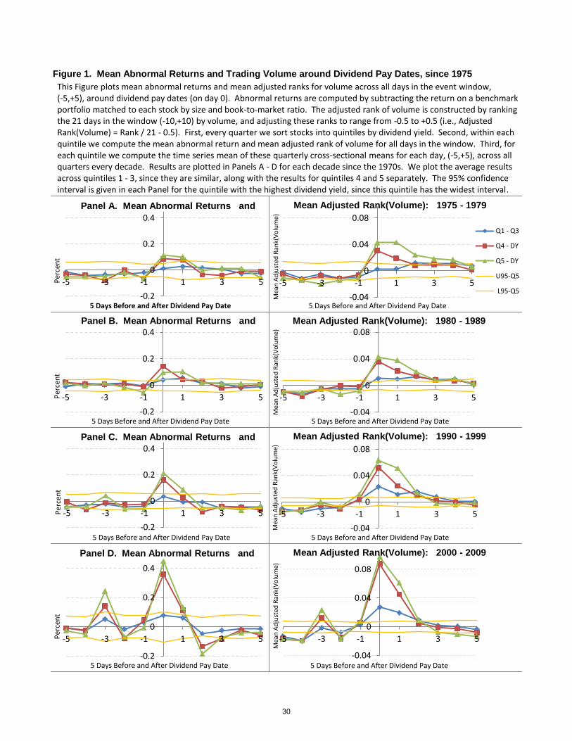
Figure 1. Mean Abnormal Returns and Trading Volume around Dividend Pay Dates, since 1975

1970

1970

1970

1970

1970

1970

1970

1970

1970

1970

1970

1970

1970

1970

1970

1970

1970

1970

1970

1970

1970

1970

5

1970

1970

1970

1970

1970

1970

This Figure plots mean abnormal returns and mean adjusted ranks for volume across all days in the event window, (-5,+5), around dividend pay dates (on day 0). Abnormal returns are computed by subtracting the return on a benchmark portfolio matched to each stock by size and book-to-market ratio. The adjusted rank of volume is constructed by ranking the 21 days in the window (-10,+10) by volume, and adjusting these ranks to range from -0.5 to +0.5 (i.e., Adjusted Rank(Volume) = Rank / 21 - 0.5). First, every quarter we sort stocks into quintiles by dividend yield. Second, within each quintile we compute the mean abnormal return and mean adjusted rank of volume for all days in the window. Third, for each quintile we compute the time series mean of these quarterly cross-sectional means for each day, (-5,+5), across all quarters every decade. Results are plotted in Panels A - D for each decade since the 1970s. We plot the average results across quintiles 1 - 3, since they are similar, along with the results for quintiles 4 and 5 separately. The 95% confidence interval is given in each Panel for the quintile with the highest dividend yield, since this quintile has the widest interval.

-0.04

0

0.04

0.08

-5 -3 -1 1 3 5

Mea

n A

dju

sted

Ran

k(V

olu

me)

5 Days Before and After Dividend Pay Date

Mean Adjusted Rank(Volume): 2000 - 2009

-0.2

0

0.2

0.4

-5 -3 -1 1 3 5Per

cen

t

5 Days Before and After Dividend Pay Date

Panel D. Mean Abnormal Returns and

-0.04

0

0.04

0.08

-5 -3 -1 1 3 5

Mea

n A

dju

sted

Ran

k(V

olu

me)

5 Days Before and After Dividend Pay Date

Mean Adjusted Rank(Volume): 1990 - 1999

-0.2

0

0.2

0.4

-5 -3 -1 1 3 5Per

cen

t

5 Days Before and After Dividend Pay Date

Panel C. Mean Abnormal Returns and

-0.04

0

0.04

0.08

-5 -3 -1 1 3 5

Mea

n A

dju

sted

Ran

k(V

olu

me)

5 Days Before and After Dividend Pay Date

Mean Adjusted Rank(Volume): 1980 - 1989

-0.2

0

0.2

0.4

-5 -3 -1 1 3 5Per

cen

t

5 Days Before and After Dividend Pay Date

Panel B. Mean Abnormal Returns and

-0.04

0

0.04

0.08

-5 -3 -1 1 3 5M

ean

Ad

just

ed R

ank(

Vo

lum

e)

5 Days Before and After Dividend Pay Date

Q1 - Q3

Q4 - DY

Q5 - DY

U95-Q5

L95-Q5

Mean Adjusted Rank(Volume): 1975 - 1979

-0.2

0

0.2

0.4

-5 -3 -1 1 3 5Per

cen

t

5 Days Before and After Dividend Pay Date

Panel A. Mean Abnormal Returns and

30

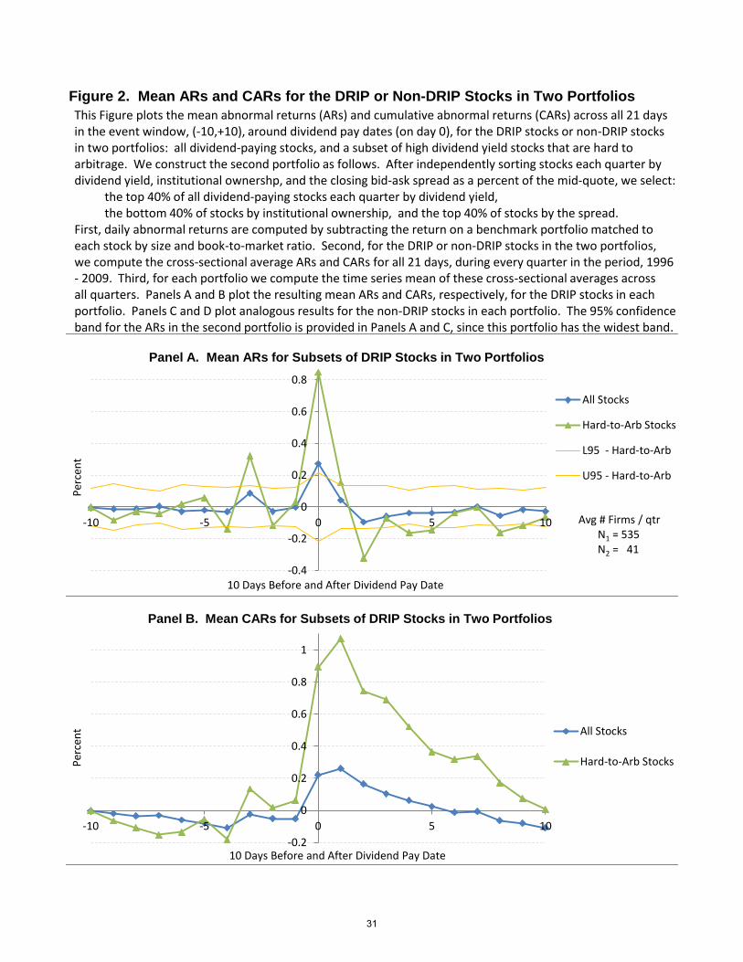
Figure 2. Mean ARs and CARs for the DRIP or Non-DRIP Stocks in Two Portfolios

1

2

3

4

5

6

7

8

9

10

-0.4

-0.2

0

0.2

0.4

0.6

0.8

-10 -5 0 5 10

Per

cen

t

10 Days Before and After Dividend Pay Date

All Stocks

Hard-to-Arb Stocks

L95 - Hard-to-Arb

U95 - Hard-to-Arb

Panel A. Mean ARs for Subsets of DRIP Stocks in Two Portfolios

Avg # Firms / qtr N1 = 535 N2 = 41

-0.2

0

0.2

0.4

0.6

0.8

1

-10 -5 0 5 10

Per

cen

t

10 Days Before and After Dividend Pay Date

All Stocks

Hard-to-Arb Stocks

Panel B. Mean CARs for Subsets of DRIP Stocks in Two Portfolios

This Figure plots the mean abnormal returns (ARs) and cumulative abnormal returns (CARs) across all 21 days in the event window, (-10,+10), around dividend pay dates (on day 0), for the DRIP stocks or non-DRIP stocks in two portfolios: all dividend-paying stocks, and a subset of high dividend yield stocks that are hard to arbitrage. We construct the second portfolio as follows. After independently sorting stocks each quarter by dividend yield, institutional ownershp, and the closing bid-ask spread as a percent of the mid-quote, we select: the top 40% of all dividend-paying stocks each quarter by dividend yield, the bottom 40% of stocks by institutional ownership, and the top 40% of stocks by the spread. First, daily abnormal returns are computed by subtracting the return on a benchmark portfolio matched to each stock by size and book-to-market ratio. Second, for the DRIP or non-DRIP stocks in the two portfolios, we compute the cross-sectional average ARs and CARs for all 21 days, during every quarter in the period, 1996 - 2009. Third, for each portfolio we compute the time series mean of these cross-sectional averages across all quarters. Panels A and B plot the resulting mean ARs and CARs, respectively, for the DRIP stocks in each portfolio. Panels C and D plot analogous results for the non-DRIP stocks in each portfolio. The 95% confidence band for the ARs in the second portfolio is provided in Panels A and C, since this portfolio has the widest band.

31

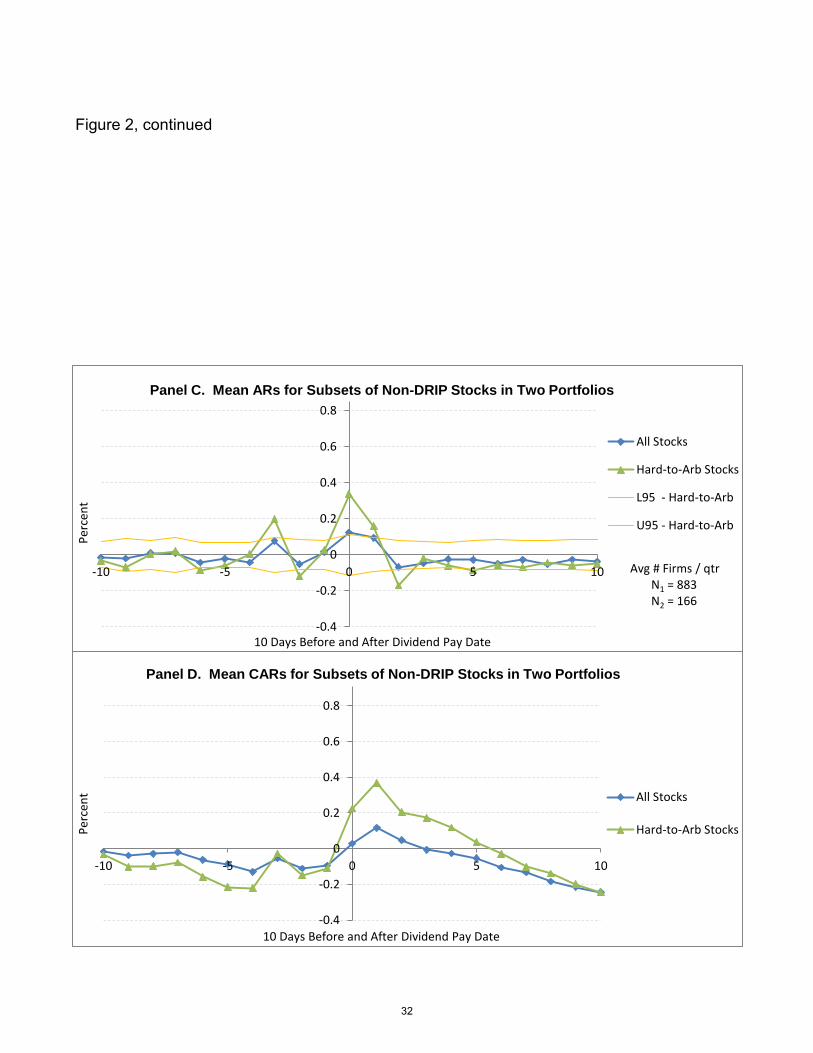
Figure 2, continued

-6

-5

-4

-3

-2

-1

0

1

2

3

4

5

6

7

8

9

10

-0.4

-0.2

0

0.2

0.4

0.6

0.8

-10 -5 0 5 10

Per

cen

t

10 Days Before and After Dividend Pay Date

All Stocks

Hard-to-Arb Stocks

L95 - Hard-to-Arb

U95 - Hard-to-Arb

Panel C. Mean ARs for Subsets of Non-DRIP Stocks in Two Portfolios

Avg # Firms / qtr N1 = 883 N2 = 166

-0.4

-0.2

0

0.2

0.4

0.6

0.8

-10 -5 0 5 10

Per

cen

t

10 Days Before and After Dividend Pay Date

All Stocks

Hard-to-Arb Stocks

Panel D. Mean CARs for Subsets of Non-DRIP Stocks in Two Portfolios

32

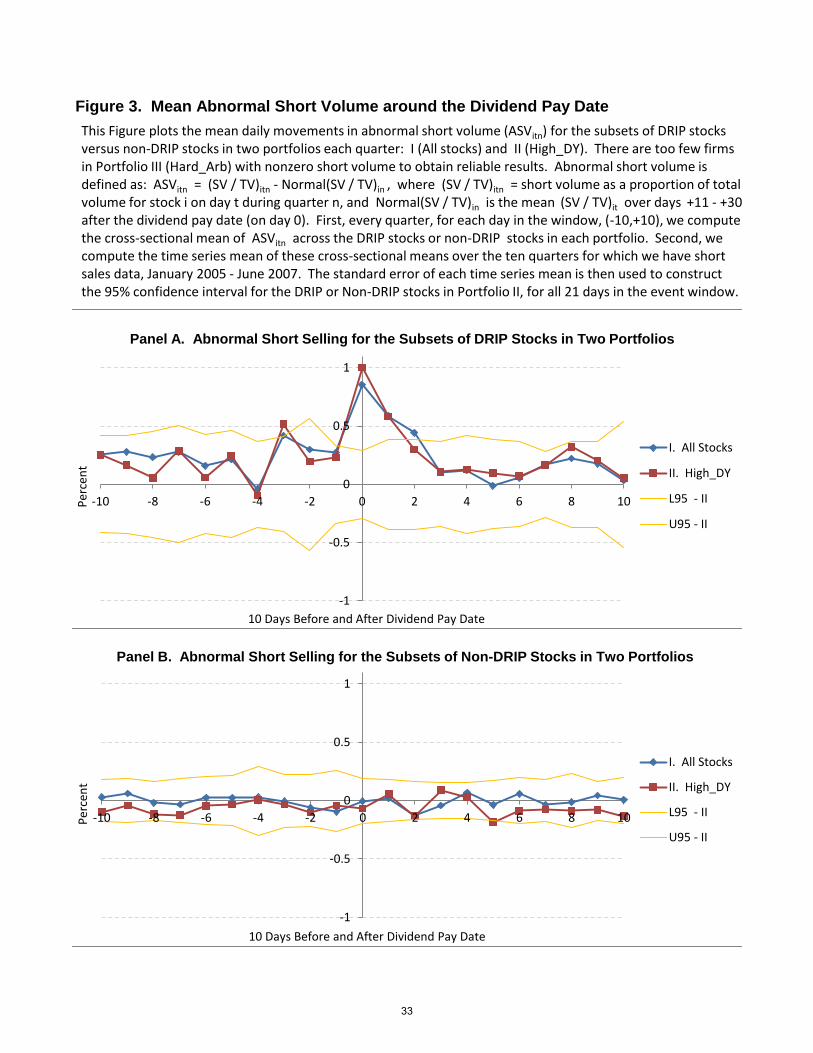
Figure 3. Mean Abnormal Short Volume around the Dividend Pay Date

-1

-0.5

0

0.5

1

-10 -8 -6 -4 -2 0 2 4 6 8 10Per

cen

t

10 Days Before and After Dividend Pay Date

I. All Stocks

II. High_DY

L95 - II

U95 - II

Panel A. Abnormal Short Selling for the Subsets of DRIP Stocks in Two Portfolios

-1

-0.5

0

0.5

1

-10 -8 -6 -4 -2 0 2 4 6 8 10Per

cen

t

10 Days Before and After Dividend Pay Date

I. All Stocks

II. High_DY

L95 - II

U95 - II

Panel B. Abnormal Short Selling for the Subsets of Non-DRIP Stocks in Two Portfolios

This Figure plots the mean daily movements in abnormal short volume (ASVitn) for the subsets of DRIP stocks versus non-DRIP stocks in two portfolios each quarter: I (All stocks) and II (High_DY). There are too few firms in Portfolio III (Hard_Arb) with nonzero short volume to obtain reliable results. Abnormal short volume is defined as: ASVitn = (SV / TV)itn - Normal(SV / TV)in , where (SV / TV)itn = short volume as a proportion of total volume for stock i on day t during quarter n, and Normal(SV / TV)in is the mean (SV / TV)it over days +11 - +30 after the dividend pay date (on day 0). First, every quarter, for each day in the window, (-10,+10), we compute the cross-sectional mean of ASVitn across the DRIP stocks or non-DRIP stocks in each portfolio. Second, we compute the time series mean of these cross-sectional means over the ten quarters for which we have short sales data, January 2005 - June 2007. The standard error of each time series mean is then used to construct the 95% confidence interval for the DRIP or Non-DRIP stocks in Portfolio II, for all 21 days in the event window.

33

-2

-2

-1

0

1

2

3

4

5

1996 1998 2000 2002 2004 2006 2008 2010

Per

cen

t

I. All Stocks

II. High_DY

III. Hard_Arb

Figure 4. Time Series of Quarterly Profits, Average of Daily Mean Abnormal Return, AR(0)n, from Holding Equally Weighted Portfolio of DRIP Stocks in Portfolios I - III

This Figure plots the quarterly time series of the average daily mean market-adjusted abnormal returns on the dividend pay date, AR(0)n, for the subsets of DRIP stocks in Portfolios I - III. Daily market-adjusted abnormal returns are obtained by subtracting the daily return on the S&P 500 index from the daily return for each stock. Every day (t) we compute the mean cross-sectional abnormal return on the dividend pay date, AR(0)t , for the subset of DRIP stocks in each portfolio that pays dividends on that date. We then compute the quarterly average of this series of mean daily abnormal returns, AR(0)t, over all days in which at least one DRIP stock in each portfolio pays a dividend. The results reflect the quarterly average one-day market-adjusted AR(0)n from three separate trading strategies that prescribe holding the DRIP stocks in each portfolio on their respective dividend pay dates during a given quarter.

Avg AR(0)/qtr: I: 0.31% II: 0.58% III: 0.92% Avg #Firms/qtr: I: 535 II: 258 III: 41

34

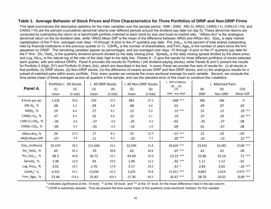
Table 1. Average Behavior of Stock Prices and Firm Characteristics for Three Portfolios of DRIP and Non-DRIP Firms

(1) (2) (3) (4) (5) (6) (8) (9)

mean (t-stat) mean (t-stat) mean (t-stat) DRIP Non-DRIP

# firms per qtr 1,418 59.0 535 37.5 883 47.5 -348 *** 286 286 0

AR(-3)in % .08 4.2 .09 4.8 .08 3.4 .01 .09 .07 .02

AR(0)in % .19 8.4 .27 9.1 .12 5.3 .15 *** .31 .12 .19 ***

CAR(0,+1)in % .27 6.4 .32 6.6 .22 5.1 .10 .37 .20 .16 ***

CAR(+2,+10)in % -.36 -3.5 -.37 -3.9 -.35 -3.2 -.02 -.35 -.27 -.08

CAR(0,+10)in % -.09 -0.7 -.05 -0.4 -.14 -1.0 .09 .01 -.07 .08. . . .

AR(ex-div)in % .26 12.3 .17 8.3 .31 12.7 -.15 *** .21 .25 -.03

AR(0) Mean Diff -.07 -3.2 .11 4.2 -.19 -7.1 .29 *** .10 -.13 .22 ***

. . . .Sizein (millions) $5,579 29.3 $11,660 24.2 $2,039 21.8 $9,620 *** $3,433 $3,581 -$148 ***

Div_Yieldin % .65 45.2 .70 49.8 .62 40.6 .07 *** .61 .61 .00

Pct_Instin-1 % 48.3 43.8 56.72 52.7 43.49 35.0 13.23 *** 53.86 53.16 .71 ***

Spreadin % 1.48 12.9 .92 10.5 1.84 13.3 -.92 *** 1.11 1.12 -.01

Log_HiLoin % 3.01 19.7 2.76 17.8 3.17 20.2 -.41 * 2.83 3.03 -.20 ***

CSHRina

% 4,316 55.1 13,036 62.3 1,625 59.8 11,411 *** 6,863 2,619 2,975 ***

Firm_Agein % 23.46 114.3 33.83 103.1 17.36 83.5 16.47 *** 28.70 20.01 8.68 ***

* indicates significance at the .10 level; ** at the .05 level; and *** at the .01 level, for the mean difference t-test in the last column.a CSHR is extremely skewed. Thus we present the time series mean of the quarterly cross-sectional medians for this variable.

Panel A.Portfolio I. All Stocks I. All DRIP Stocks I. All Non-DRIP Stocks

DRIP - Non-DRIP

(7)

Mean Diff

I. Matched Pairs

(10)

I. Diff of Means

(3) - (5)

This table summarizes the descriptive statistics for the main variables over the sample period, 1996 - 2009. AR(-3), AR(0), CAR(0,+1), CAR(+2,+10), and CAR(0,+10) are the percent (cumulative) abnormal returns over different periods around the dividend pay date (on day 0). These abnormal returns are computed by subtracting the return on a benchmark portfolio matched to each stock by size and book-to-market ratio. "AR(ex-div)" is the analogous abnormal return on the ex-dividend date, while "AR(0) Mean Diff" is the mean of the difference between AR(0) and AR(ex-div). Sizein is daily market capitalization of the ith firm, averaged over days -10 through -6 prior to the nth quarterly pay date. Pct_Instin-1 is the percent of total shares outstanding held by financial institutions in the previous quarter (n-1). CSHRin is the number of shareholders, and Firm_Agein is the number of years since the firm appeared on CRSP. The remaining variables appear as percentages, and are averaged over days -10 through -6 prior to the nth quarterly pay date for the ith firm: Div_Yieldin is the quarterly dividend amount divided by the daily closing price; Spreadin is the daily closing spread divided by the share price; and Log_HiLoin is the natural log of the ratio of the daily high to the daily low. Panels A - C give the results for three different portfolios of stocks selected each quarter, with and without DRIPs. Panel A provides the results for Portfolio I (All dividend-paying stocks), while Panels B and C present the results for Portfolio II (High_DY) and Portfolio III (Hard_Arb), which are described in the text. In every Panel we provide five sets of results for: (i) all stocks in that portfolio, (ii) DRIP stocks, (iii) Non-DRIP stocks, (iv) the difference of means across DRIP and Non-DRIP stocks, and (v) the analogous results for a subset of matched pairs within every portfolio. First, every quarter we compute the cross-sectional average for each variable. Second, we compute the time series mean of these averages across all quarters in the sample, and use the standard error of this mean to construct the t-statistics.

35

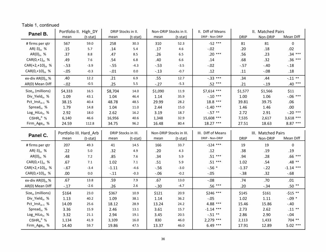
mean (t-stat) mean (t-stat) mean (t-stat) DRIP Non-DRIP

# firms per qtr 567 59.0 258 30.3 310 52.3 -52 *** 81 81 0

AR(-3)in % .15 5.7 .14 5.4 .17 4.6 -.02 .20 .18 .02AR(0)in % .37 8.8 .47 8.5 .26 6.5 .20 *** .56 .23 .34 ***

CAR(0,+1)in % .49 7.6 .54 6.8 .40 6.6 .14 .68 .32 .36 ***

CAR(+2,+10)in % -.53 -3.9 -.55 -4.3 -.53 -3.5 -.02 -.57 -.40 -.18CAR(0,+10)in % -.05 -0.3 -.01 0.0 -.13 -0.7 .12 .11 -.08 .18

. . . . . .ex-div AR(0)in % .40 12.2 .21 6.9 .55 12.7 -.33 *** .34 .44 -.11 **

AR(0) Mean Diff -.02 -0.5 .25 5.5 -.27 -5.3 .52 *** .21 -.19 .40 ***. . . . . .

Sizein (millions) $4,333 16.5 $8,704 14.0 $1,090 11.9 $7,614 *** $1,577 $1,566 $11

Div_Yieldin % 1.09 43.1 1.04 46.4 1.14 35.9 -.10 *** 1.00 1.06 -.06 ***

Pct_Instin-1 % 38.15 40.4 48.78 48.5 29.99 28.2 18.8 *** 39.81 39.75 .06Spreadin % 1.79 14.8 1.04 11.0 2.44 15.0 -1.40 *** 1.46 1.46 .00

Log_HiLoin % 2.92 18.0 2.62 16.2 3.19 18.7 -.57 ** 2.72 2.91 -.20 ***

CSHRina

% 6,140 46.6 16,956 40.6 1,348 32.9 15,608 *** 7,535 2,617 3,618 ***

Firm_Agein % 24.59 112.8 34.75 96.2 16.48 80.4 18.27 *** 27.51 18.63 8.87 ***

mean (t-stat) mean (t-stat) mean (t-stat) DRIP Non-DRIP

# firms per qtr 207 49.3 41 14.5 166 33.7 -124 *** 19 19 0

AR(-3)in % .22 5.0 .32 4.9 .20 4.3 .12 .38 .19 .19

AR(0)in % .48 7.2 .85 7.6 .34 5.9 .51 *** .94 .28 .66 ***

CAR(0,+1)in % .67 7.1 1.02 7.1 .51 5.9 .51 *** 1.02 .54 .48 **

CAR(+2,+10)in % -.67 -3.4 -1.11 -4.6 -.56 -3.0 -.56 * -1.37 -.22 -1.14 ***

CAR(0,+10)in % .00 0.0 -.11 -0.3 -.06 -0.2 -.05 -.38 .32 -.68. . . . . .

ex-div AR(0)in % .67 13.8 .59 7.9 .67 13.0 -.08 .74 .70 .01

AR(0) Mean Diff -.17 -2.6 .26 2.6 -.30 -4.7 .56 *** .20 -.34 .50 **. . . . . .

Sizein (millions) $164 23.0 $367 10.9 $121 20.9 $246 *** $145 $161 -$15 **

Div_Yieldin % 1.13 40.2 1.09 38.1 1.14 36.2 -.05 1.02 1.11 -.09 *

Pct_Instin-1 % 14.09 25.6 18.12 28.9 13.24 24.2 4.88 *** 15.46 15.86 -.40Spreadin % 3.36 15.9 2.46 13.1 3.61 15.7 -1.14 *** 2.73 2.62 .11 **

Log_HiLoin % 3.32 21.1 2.94 19.1 3.45 20.5 -.51 ** 2.86 2.90 -.04CSHRin

a % 1,134 41.9 3,109 16.0 830 46.0 2,279 *** 2,113 1,433 704 **

Firm_Agein % 14.40 59.7 19.86 47.5 13.37 46.0 6.49 *** 17.91 12.89 5.02 ***

Panel B.

Panel C.

Table 1, continued

Portfolio III. Hard_Arb

Portfolio II. High_DY

DRIP - Non-DRIP

DRIP Stocks in II. Non-DRIP Stocks in II.

DRIP Stocks in III. Non-DRIP Stocks in III.

II. Diff of Means

III. Matched PairsMean Diff

DRIP - Non-DRIP

III. Diff of Means

II. Matched PairsMean Diff

36

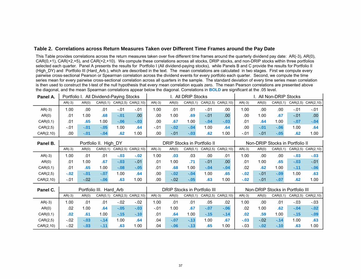
Panel A.

AR(-3) 1.00 .00 .01 -.01 -.01 1.00 .01 .01 -.01 .00 1.00 .00 .00 -.01 -.01

AR(0) .01 1.00 .68 -.01 .00 .00 1.00 .69 -.01 .00 .00 1.00 .67 -.01 .00

CAR(0,1) .01 .65 1.00 -.06 -.03 .00 .67 1.00 -.04 -.03 .01 .64 1.00 -.07 -.04

CAR(2,5) -.01 -.01 -.05 1.00 .64 -.01 -.02 -.04 1.00 .64 .00 -.01 -.06 1.00 .64

CAR(2,10) .00 -.01 -.04 .62 1.00 .00 -.01 -.03 .62 1.00 -.01 -.01 -.05 .62 1.00

Panel B.

AR(-3) 1.00 .01 .01 -.03 -.02 1.00 .03 .03 .00 .01 1.00 .00 .00 -.03 -.03

AR(0) .01 1.00 .67 -.03 -.01 .01 1.00 .71 -.01 .00 .01 1.00 .65 -.03 -.01

CAR(0,1) .01 .65 1.00 -.08 -.05 .01 .68 1.00 -.04 -.04 .02 .62 1.00 -.11 -.06

CAR(2,5) -.02 -.01 -.07 1.00 .64 .00 -.02 -.04 1.00 .65 -.02 -.01 -.09 1.00 .63

CAR(2,10) -.01 -.02 -.06 .63 1.00 .00 -.02 -.05 .63 1.00 -.02 -.01 -.07 .62 1.00

Panel C.

AR(-3) 1.00 .01 .01 -.02 -.02 1.00 .01 .01 .05 .02 1.00 .00 .01 -.03 -.03

AR(0) .02 1.00 .64 -.05 -.03 -.01 1.00 .67 -.07 -.06 .02 1.00 .62 -.04 -.02

CAR(0,1) .02 .61 1.00 -.15 -.10 .01 .64 1.00 -.15 -.14 .02 .59 1.00 -.15 -.09

CAR(2,5) -.02 -.03 -.14 1.00 .64 .04 -.07 -.13 1.00 .67 -.03 -.02 -.14 1.00 .63

CAR(2,10) -.02 -.03 -.11 .63 1.00 .04 -.06 -.13 .65 1.00 -.03 -.02 -.10 .63 1.00

Table 2. Correlations across Return Measures Taken over Different Time Frames around the Pay Date

Portfolio I. All Dividend-Paying Stocks

CAR(0,1)AR(-3) AR(0) CAR(2,5)

I. All DRIP Stocks

AR(-3) AR(0) CAR(0,1) CAR(2,5)

I. All Non-DRIP Stocks

AR(-3) AR(0) CAR(0,1) CAR(2,5)

Portfolio II. High_DY DRIP Stocks in Portfolio II Non-DRIP Stocks in Portfolio II

CAR(2,10) CAR(2,10) CAR(2,10)

AR(-3) AR(0) CAR(0,1) CAR(2,5) CAR(2,10) AR(-3) AR(0) CAR(0,1) CAR(2,5) CAR(2,10) CAR(2,10)

AR(0) CAR(0,1)

AR(-3) AR(0) CAR(0,1)

CAR(2,5)

CAR(2,5)

CAR(2,10)

Portfolio III. Hard_Arb DRIP Stocks in Portfolio III Non-DRIP Stocks in Portfolio III

AR(-3) AR(0) CAR(0,1) CAR(2,5) AR(-3) AR(0) CAR(0,1) CAR(2,5) AR(-3)CAR(2,10) CAR(2,10)

This Table provides correlations across the return measures taken over five different time frames around the quarterly dividend pay date: AR(-3), AR(0), CAR(0,+1), CAR(+2,+5), and CAR(+2,+10). We compute these correlations across all stocks, DRIP stocks, and non-DRIP stocks within three portfolios selected each quarter. Panel A presents the results for Portfolio I (All dividend-paying stocks), while Panels B and C provide the results for Portfolio II (High_DY) and Portfolio III (Hard_Arb.), which are described in the text. The mean correlations are calculated in two stages. First we compute every pairwise cross-sectional Pearson or Spearman correlation across the dividend events for every portfolio each quarter. Second, we compute the time series mean for every pairwise cross-sectional correlation across all quarters in the sample. The standard deviation of every time series mean correlation is then used to construct the t-test of the null hypothesis that every mean correlation equals zero. The mean Pearson correlations are presented above the diagonal, and the mean Spearman correlations appear below the diagonal. Correlations in BOLD are significant at the .05 level.

37

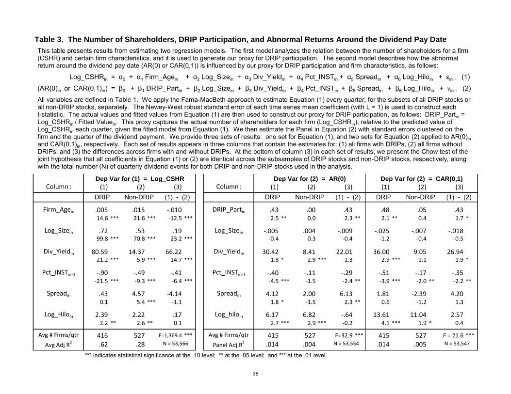
Table 3. The Number of Shareholders, DRIP Participation, and Abnormal Returns Around the Dividend Pay Date

Column : (1) (2) (3) Column : (1) (2) (3) (1) (2) (3)

Firm_Agein .005 .015 -.010 DRIP_Partin .43 .00 .43 .48 .05 .43 14.6 *** 21.6 *** -12.5 *** 2.5 ** 0.0 2.3 ** 2.1 ** 0.4 1.7 *

Log_Sizein .72 .53 .19 Log_Sizein -.005 .004 -.009 -.025 -.007 -.018 99.8 *** 70.8 *** 23.2 *** -0.4 0.3 -0.4 -1.2 -0.4 -0.5

Div_Yieldin 80.59 14.37 66.22 Div_Yieldin 30.42 8.41 22.01 36.00 9.05 26.9421.2 *** 5.9 *** 14.7 *** 1.8 * 2.9 *** 1.3 2.9 *** 1.1 1.9 *

Pct_INSTin-1 -.90 -.49 -.41 Pct_INSTin-1 -.40 -.11 -.29 -.51 -.17 -.35-21.5 *** -9.3 *** -6.4 *** -4.5 *** -1.5 -2.4 ** -3.9 *** -2.0 ** -2.2 **

Spreadin .43 4.57 -4.14 Spreadin 4.12 2.00 6.13 1.81 -2.39 4.200.1 5.4 *** -1.1 1.8 * -1.5 2.3 ** 0.6 -1.2 1.3

Log_Hiloin 2.39 2.22 .17 Log_hiloin 6.17 6.82 -.64 13.61 11.04 2.572.2 ** 2.6 ** 0.1 2.7 *** 2.9 *** -0.2 4.1 *** 1.9 * 0.4

Avg # Firms/qtr 416 527 F=1,369.4 *** Avg # Firms/qtr 415 527 F=32.9 *** 415 527 F = 21.6 ***

Avg Adj R2 .62 .28 Panel Adj R2 .014 .004 .014 .005

*** indicates statistical significance at the .10 level; ** at the .05 level; and *** at the .01 level.

Dep Var for (2) = CAR(0,1)

N = 53,566 N = 53,554 N = 53,547

DRIP Non-DRIP (1) - (2)DRIP Non-DRIP (1) - (2)DRIP Non-DRIP (1) - (2)

Dep Var for (1) = Log_CSHR Dep Var for (2) = AR(0)

This table presents results from estimating two regression models. The first model analyzes the relation between the number of shareholders for a firm (CSHR) and certain firm characteristics, and it is used to generate our proxy for DRIP participation. The second model describes how the abnormal return around the dividend pay date (AR(0) or CAR(0,1)) is influenced by our proxy for DRIP participation and firm characteristics, as follows:

Log_CSHRin = α0 + α1 Firm_Agein + α2 Log_Sizein + α3 Div_Yieldin + α4 Pct_INSTin + α5 Spreadin + α6 Log_Hiloin + ɛin , (1)

(AR(0)in or CAR(0,1)in) = β0 + β1 DRIP_Partin + β2 Log_Sizein + β3 Div_Yieldin + β4 Pct_INSTin + β5 Spreadin + β6 Log_Hiloin + νin . (2)

All variables are defined in Table 1. We apply the Fama-MacBeth approach to estimate Equation (1) every quarter, for the subsets of all DRIP stocks or all non-DRIP stocks, separately. The Newey-West robust standard error of each time series mean coefficient (with L = 1) is used to construct each t-statistic. The actual values and fitted values from Equation (1) are then used to construct our proxy for DRIP participation, as follows: DRIP_Partin = Log_CSHRin / Fitted Valuein. This proxy captures the actual number of shareholders for each firm (Log_CSHRin), relative to the predicted value of Log_CSHRin each quarter, given the fitted model from Equation (1). We then estimate the Panel in Equation (2) with standard errors clustered on the firm and the quarter of the dividend payment. We provide three sets of results: one set for Equation (1), and two sets for Equation (2) applied to AR(0)in and CAR(0,1)in, respectively. Each set of results appears in three columns that contain the estimates for: (1) all firms with DRIPs, (2) all firms without DRIPs, and (3) the differences across firms with and without DRIPs. At the bottom of column (3) in each set of results, we present the Chow test of the joint hypothesis that all coefficients in Equation (1) or (2) are identical across the subsamples of DRIP stocks and non-DRIP stocks, respectively, along with the total number (N) of quarterly dividend events for both DRIP and non-DRIP stocks used in the analysis.

38

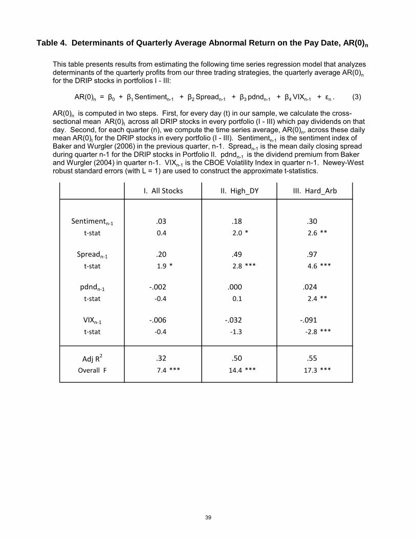
Sentimentn-1 .03 .18 .30

t-stat 0.4 2.0 * 2.6 **

Spreadn-1 .20 .49 .97

t-stat 1.9 * 2.8 *** 4.6 ***

pdndn-1 -.002 .000 .024

t-stat -0.4 0.1 2.4 **

VIXn-1 -.006 -.032 -.091

t-stat -0.4 -1.3 -2.8 ***

Adj R2 .32 .50 .55

Overall F 7.4 *** 14.4 *** 17.3 ***

I. All Stocks II. High_DY III. Hard_Arb

Table 4. Determinants of Quarterly Average Abnormal Return on the Pay Date, AR(0)n

This table presents results from estimating the following time series regression model that analyzes determinants of the quarterly profits from our three trading strategies, the quarterly average AR(0)n for the DRIP stocks in portfolios I - III:

AR(0)n = β0 + β1 Sentimentn-1 + β2 Spreadn-1 + β3 pdndn-1 + β4 VIXn-1 + εn . (3)

AR(0)n is computed in two steps. First, for every day (t) in our sample, we calculate the cross-sectional mean AR(0)t across all DRIP stocks in every portfolio (I - III) which pay dividends on that day. Second, for each quarter (n), we compute the time series average, AR(0)n, across these daily mean AR(0)t for the DRIP stocks in every portfolio (I - III). Sentimentn-1 is the sentiment index of Baker and Wurgler (2006) in the previous quarter, n-1. Spreadn-1 is the mean daily closing spread during quarter n-1 for the DRIP stocks in Portfolio II. pdndn-1 is the dividend premium from Baker and Wurgler (2004) in quarter n-1. VIXn-1 is the CBOE Volatility Index in quarter n-1. Newey-West robust standard errors (with L = 1) are used to construct the approximate t-statistics.

39

40

Appendix A. Excerpts from Dividend Reinvestment Plans (DRIPs)

The following excerpts exemplify the relevant details common in DRIP documentation.

1. H.B. Fuller Company DRIP Document (2011), selected excerpts:

“As the Plan Administrator, Wells Fargo Shareowner Services, a division of Wells Fargo

Bank, N.A., (the Plan ‘Administrator’) offers investors a simple and convenient method of

investing in H.B. Fuller Company common stock. The Plan Administrator will apply all of the

participants’ designated dividends … to purchase whole and fractional shares acquired under the

Dividend Reinvestment Plan. Such purchases may be made on any securities exchange where

such shares are traded, in the over-the-counter market or in negotiated transactions, and may be

on such terms as to price, delivery and otherwise as the Plan Administrator may determine.

Dividends are invested as soon as administratively possible on or following the dividend

payable date, generally within five (5) trading days. In the case of each purchase, the price at

which the Plan Administrator shall be deemed to have acquired H.B. Fuller common stock for

the participant’s account shall be the weighted average price of all shares purchased plus any per

share fees. Depending on the number of shares being purchased and current trading volumes in

the shares, purchases may be executed in multiple transactions that may occur on more than one

day.”

2. Carnival Corporation DRIP Document (2007), selected excerpts:

“The shares of Carnival Corporation common stock purchased under the (Dividend

Reinvestment) Plan may be newly issued shares or shares purchased for participants in the open

market, at Carnival Corporation’s option. The Plan currently provides that shares purchased for

participants with reinvested dividends will be purchased at fair market value, as determined in

the Plan.

41

WHO ADMINISTERS THE PLAN?

Computershare Trust Company, N.A. (the ‘Agent’), a bank unaffiliated with Carnival

Corporation, administers the Plan. The Agent arranges for the custody of share certificates, keeps

records, sends statements of account to participants, and makes purchases of shares of Carnival

Corporation common stock under the Plan for the accounts of participants. The Agent will send

each participant a statement of his or her account under the Plan as soon as practicable following

each purchase of shares of Carnival Corporation common stock. Each statement will show (a)

any dividends credited; (b) plan shares purchased and fractional shares allocated; (c) the cost per

share of the purchased shares and fractional shares; (d) the number of whole shares for which

certificates have been issued, if any; and the beginning and ending balances of whole shares and

fractional shares … The Agent will also serve as custodian of shares purchased under the Plan to

protect participants from loss, theft or destruction of stock certificates.

WHAT IS THE SOURCE OF SHARES PURCHASED UNDER THE PLAN?

Shares purchased under the Plan will come from the authorized and unissued shares of

the Carnival Corporation common stock or from shares purchased on the open market by the

Agent, as determined by Carnival Corporation.

With respect to any open market purchases made under the Plan, the Agent will have full

discretion as to all matters relating to purchases, including determination of the number of

shares, if any, to be purchased on any day, the time of day, the price paid for such shares, the

markets in which such shares are to be purchased …

WHEN WILL FUNDS BE INVESTED UNDER THE PLAN?

If shares are purchased from Carnival Corporation, the purchases will be made on the

dividend payment date and such shares will be credited to participants’ accounts on the dividend

42

payment date. If shares are to be purchased in the open market, the Agent is to use its best efforts

to apply all funds received by it to the purchase of shares within 30 days of the receipt of such

funds from Carnival Corporation …

WHAT IS THE PURCHASE PRICE OF THE SHARES?

If the Carnival Corporation common stock is purchased from Carnival Corporation, the

price per share … will be the closing price for the Carnival Corporation common stock on the

NYSE Composite Tape on the dividend payment date, as reported in THE WALL STREET

JOURNAL or other authoritative source. The price per share for open market purchases will be

the weighted average price paid by the Agent for all shares of Carnival Corporation common

stock purchased by it for participants in the Plan through negotiation with the seller. No share of

Carnival Corporation common stock will be purchased at a price in excess of current market

prices at the time of purchase.”

Appendix B. Time Series Means of Cross-Sectional Medians for the Variables

In this appendix we duplicate the analysis in Table 1, but we analyze the average behavior of the

cross-section medians of the main variables each quarter, rather than the cross-sectional means.

This evidence is presented in Table B.1, and is generally robust with respect to the analysis in

Table 1. This outcome indicates that our main results are not due to outliers.

Appendix C. The Intraday Price Pattern on the Dividend Pay Date

In this appendix we examine the intraday pattern in price movements on the dividend pay date,

for the subsets of DRIP stocks in Portfolios I - III. This analysis reveals whether investors (or

their transfer agents) tend to exert price pressure at certain times on the day that dividend funds

are distributed. We analyze intraday midquotes at five-minute intervals for the first and last 30

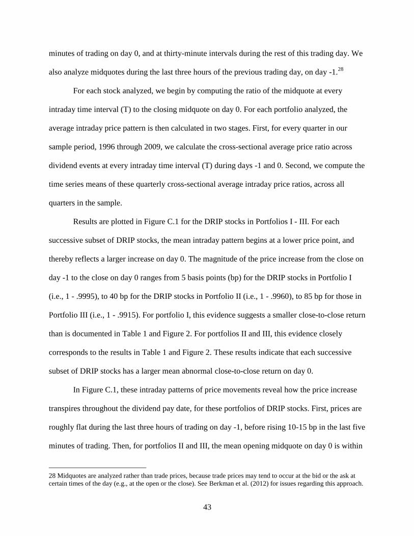
43

minutes of trading on day 0, and at thirty-minute intervals during the rest of this trading day. We

also analyze midquotes during the last three hours of the previous trading day, on day -1.28

For each stock analyzed, we begin by computing the ratio of the midquote at every

intraday time interval (T) to the closing midquote on day 0. For each portfolio analyzed, the

average intraday price pattern is then calculated in two stages. First, for every quarter in our

sample period, 1996 through 2009, we calculate the cross-sectional average price ratio across

dividend events at every intraday time interval (T) during days -1 and 0. Second, we compute the

time series means of these quarterly cross-sectional average intraday price ratios, across all

quarters in the sample.

Results are plotted in Figure C.1 for the DRIP stocks in Portfolios I - III. For each

successive subset of DRIP stocks, the mean intraday pattern begins at a lower price point, and

thereby reflects a larger increase on day 0. The magnitude of the price increase from the close on

day -1 to the close on day 0 ranges from 5 basis points (bp) for the DRIP stocks in Portfolio I

(i.e., 1 - .9995), to 40 bp for the DRIP stocks in Portfolio II (i.e., 1 - .9960), to 85 bp for those in

Portfolio III (i.e., 1 - .9915). For portfolio I, this evidence suggests a smaller close-to-close return

than is documented in Table 1 and Figure 2. For portfolios II and III, this evidence closely

corresponds to the results in Table 1 and Figure 2. These results indicate that each successive

subset of DRIP stocks has a larger mean abnormal close-to-close return on day 0.

In Figure C.1, these intraday patterns of price movements reveal how the price increase

transpires throughout the dividend pay date, for these portfolios of DRIP stocks. First, prices are

roughly flat during the last three hours of trading on day -1, before rising 10-15 bp in the last five

minutes of trading. Then, for portfolios II and III, the mean opening midquote on day 0 is within

28 Midquotes are analyzed rather than trade prices, because trade prices may tend to occur at the bid or the ask at

certain times of the day (e.g., at the open or the close). See Berkman et al. (2012) for issues regarding this approach.

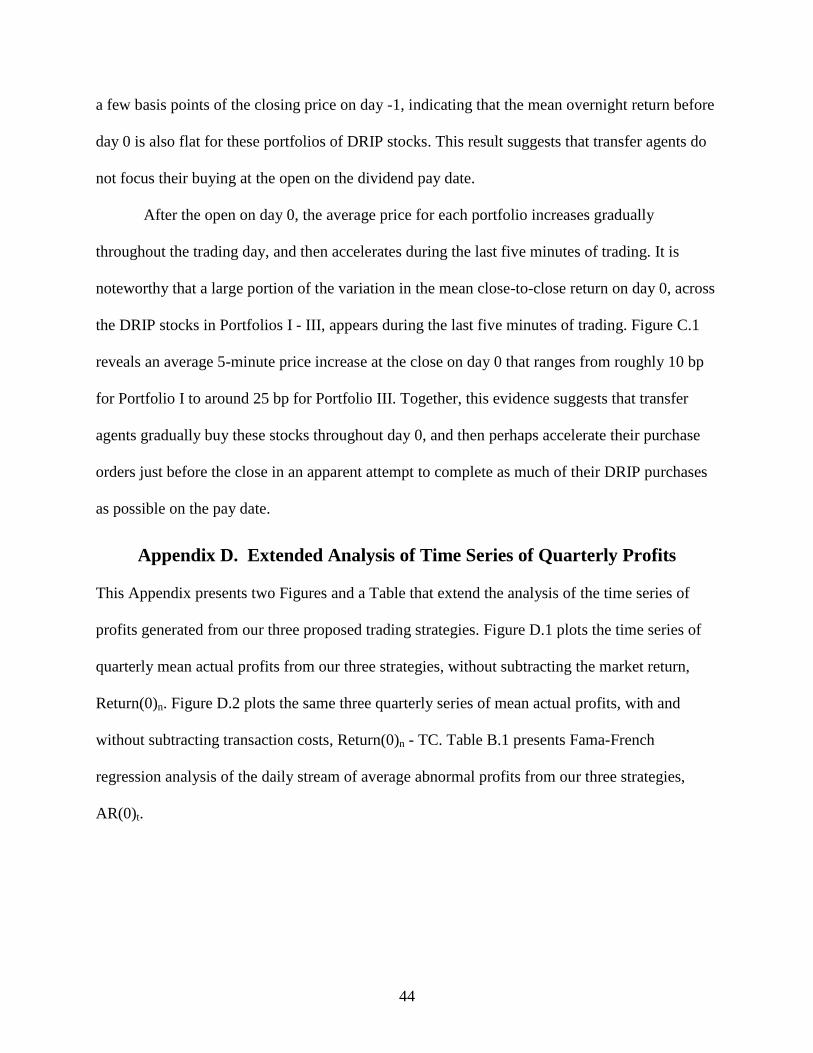
44

a few basis points of the closing price on day -1, indicating that the mean overnight return before

day 0 is also flat for these portfolios of DRIP stocks. This result suggests that transfer agents do

not focus their buying at the open on the dividend pay date.

After the open on day 0, the average price for each portfolio increases gradually

throughout the trading day, and then accelerates during the last five minutes of trading. It is

noteworthy that a large portion of the variation in the mean close-to-close return on day 0, across

the DRIP stocks in Portfolios I - III, appears during the last five minutes of trading. Figure C.1

reveals an average 5-minute price increase at the close on day 0 that ranges from roughly 10 bp

for Portfolio I to around 25 bp for Portfolio III. Together, this evidence suggests that transfer

agents gradually buy these stocks throughout day 0, and then perhaps accelerate their purchase

orders just before the close in an apparent attempt to complete as much of their DRIP purchases

as possible on the pay date.

Appendix D. Extended Analysis of Time Series of Quarterly Profits

This Appendix presents two Figures and a Table that extend the analysis of the time series of

profits generated from our three proposed trading strategies. Figure D.1 plots the time series of

quarterly mean actual profits from our three strategies, without subtracting the market return,

Return(0)n. Figure D.2 plots the same three quarterly series of mean actual profits, with and

without subtracting transaction costs, Return(0)n - TC. Table B.1 presents Fama-French

regression analysis of the daily stream of average abnormal profits from our three strategies,

AR(0)t.

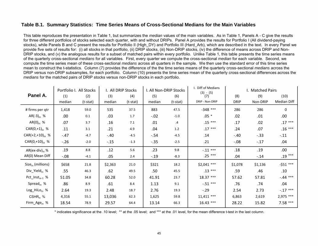
Table B.1. Summary Statistics: Time Series Means of Cross-Sectional Medians for the Main Variables

(1) (2) (3) (4) (5) (6) (8) (9)

median (t-stat) median (t-stat) median (t-stat) DRIP Non-DRIP

# firms per qtr 1,418 59.0 535 37.5 883 47.5 -348 *** 286 286 0

AR(-3)in % .00 0.1 .03 1.7 -.02 -1.0 .05 * .02 .01 .00

AR(0)in % .07 3.7 .16 7.1 .01 .4 .15 *** .17 .02 .17 ***

CAR(0,+1)in % .11 3.1 .21 4.9 .04 1.2 .17 *** .24 .07 .16 ***

CAR(+2,+10)in % -.47 -4.7 -.40 -4.5 -.54 -4.5 .14 -.40 -.33 -.11

CAR(0,+10)in % -.26 -2.0 -.15 -1.3 -.35 -2.5 .21 -.08 -.17 .04. . . . . . . . .

AR(ex-div)in % .19 8.8 .12 5.6 .23 9.8 -.11 *** .18 .19 .00

AR(0) Mean Diff -.08 -4.1 .05 2.4 -.19 -8.3 .25 *** .04 -.14 .19 ***

. . . . . . . . .Sizein (millions) $658 21.8 $2,363 21.0 $321 18.2 $2,041 *** $1,078 $1,136 -$51 ***

Div_Yieldin % .55 46.3 .62 49.5 .50 45.5 .13 *** .59 .46 .10

Pct_Instin-1 % 51.05 34.8 60.28 52.0 41.91 23.7 18.37 *** 57.62 57.81 -.44 ***

Spreadin % .86 8.9 .61 8.4 1.13 9.1 -.51 *** .76 .74 .04

Log_HiLoin % 2.64 19.3 2.48 18.7 2.76 19.3 -.29 2.54 2.73 -.17 ***

CSHRin % 4,316 55.1 13,036 62.3 1,625 59.8 11,411 *** 6,863 2,619 2,975 ***

Firm_Agein % 18.54 78.9 29.57 64.4 13.14 66.3 16.43 *** 28.22 15.82 7.58 ***

* indicates significance at the .10 level; ** at the .05 level; and *** at the .01 level, for the mean difference t-test in the last column.

I. Matched Pairs

(10)

I. Diff of Medians

(3) - (5)(7)

Median Diff

I. All DRIP Stocks I. All Non-DRIP Stocks

DRIP - Non-DRIP

Panel A.Portfolio I. All Stocks

This table reproduces the presentation in Table 1, but summarizes the median values of the main variables. As in Table 1, Panels A - C give the results for three different portfolios of stocks selected each quarter, with and without DRIPs. Panel A provides the results for Portfolio I (All dividend-paying stocks), while Panels B and C present the results for Portfolio II (High_DY) and Portfolio III (Hard_Arb), which are described in the text. In every Panel we provide five sets of results for: (i) all stocks in that portfolio, (ii) DRIP stocks, (iii) Non-DRIP stocks, (iv) the difference of means across DRIP and Non-DRIP stocks, and (v) the analogous results for a subset of matched pairs within every portfolio. Unlike Table 1, this table presents the time series means of the quarterly cross-sectional medians for all variables. First, every quarter we compute the cross-sectional median for each variable. Second, we compute the time series mean of these cross-sectional medians across all quarters in the sample. We then use the standard error of this time series mean to construct the t-statistics. Column (7) provides the difference of the the time series means of the quarterly cross-sectional medians across the DRIP versus non-DRIP subsamples, for each portfolio. Column (10) presents the time series mean of the quarterly cross-sectional differences across the medians for the matched pairs of DRIP stocks versus non-DRIP stocks in each portfolio.

45

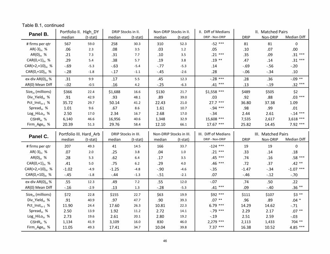
median (t-stat) median (t-stat) median (t-stat) DRIP Non-DRIP

# firms per qtr 567 59.0 258 30.3 310 52.3 -52 *** 81 81 0

AR(-3)in % .06 2.3 .08 3.5 .03 1.2 .05 .10 .07 .00AR(0)in % .21 7.3 .31 7.7 .10 3.5 .21 *** .35 .09 .31 ***

CAR(0,+1)in % .29 5.4 .38 5.7 .19 3.8 .19 ** .47 .14 .31 ***

CAR(+2,+10)in % -.69 -5.3 -.63 -5.4 -.77 -5.3 .14 -.69 -.56 -.20CAR(0,+10)in % -.28 -1.8 -.17 -1.1 -.45 -2.6 .28 -.06 -.34 .10

. . . . . . . . .ex-div AR(0)in % .31 9.9 .17 5.5 .45 12.3 -.28 *** .28 .36 -.09 **

AR(0) Mean Diff -.02 -0.5 .16 4.2 -.25 -6.3 .41 *** .13 -.19 .32 ***. . . . . . . . .

Sizein (millions) $366 22.4 $1,688 16.6 $130 21.7 $1,558 *** $489 $505 $2

Div_Yieldin % .91 42.9 .93 48.1 .89 39.0 .03 .92 .88 .03 ***

Pct_Instin-1 % 35.72 29.7 50.14 41.2 22.43 21.0 27.7 *** 36.80 37.38 1.09Spreadin % 1.01 9.6 .67 8.6 1.61 10.7 -.94 *** .98 .99 .01

Log_HiLoin % 2.50 17.0 2.34 16.7 2.68 17.0 -.34 2.44 2.61 -.14 ***

CSHRin % 6,140 46.6 16,956 40.6 1,348 32.9 15,608 *** 7,535 2,617 3,618 ***

Firm_Agein % 20.39 51.3 29.76 58.4 12.10 66.1 17.67 *** 25.82 14.45 7.92 ***

median (t-stat) median (t-stat) median (t-stat) DRIP Non-DRIP

# firms per qtr 207 49.3 41 14.5 166 33.7 -124 *** 19 19 0

AR(-3)in % .07 2.0 .25 3.8 .04 1.0 .21 *** .33 .14 .18AR(0)in % .28 5.3 .62 6.4 .17 3.5 .45 *** .74 .16 .58 ***

CAR(0,+1)in % .41 5.0 .75 6.2 .29 4.0 .46 *** .72 .37 .42 **

CAR(+2,+10)in % -1.02 -4.9 -1.25 -4.8 -.90 -4.6 -.35 -1.47 -.34 -1.07 ***

CAR(0,+10)in % -.45 -1.8 -.44 -1.3 -.51 -2.1 .07 -.46 -.12 -.70. . . . . . . . .ex-div AR(0)in % .55 12.3 .49 7.2 .55 12.0 -.07 .74 .50 .22

AR(0) Mean Diff -.16 -2.9 .13 1.3 -.28 -5.3 .41 *** .09 -.40 .36 **. . . . . . . . .Sizein (millions) $72 22.8 $155 22.7 $63 19.9 $92 *** $111 $107 $3 **

Div_Yieldin % .91 40.9 .97 47.7 .90 39.3 .07 ** .96 .89 .04 *

Pct_Instin-1 % 11.90 24.4 17.60 26.3 10.81 22.3 6.79 *** 14.29 14.62 -.71Spreadin % 2.50 13.9 1.92 11.2 2.72 14.1 -.79 *** 2.29 2.17 .07 **

Log_HiLoin % 2.73 19.6 2.61 20.1 2.80 19.2 -.19 2.51 2.59 -.03CSHRin

% 1,134 41.9 3,109 16.0 830 46.0 2,279 *** 2,113 1,433 704 **

Firm_Agein % 11.05 49.3 17.41 34.7 10.04 39.8 7.37 *** 16.38 10.52 4.85 ***

II. Matched PairsMedian Diff

III. Matched PairsMedian Diff

DRIP - Non-DRIP

III. Diff of MediansDRIP - Non-DRIP

DRIP Stocks in II. Non-DRIP Stocks in II.

DRIP Stocks in III. Non-DRIP Stocks in III.

II. Diff of MediansPanel B.

Panel C.

Table B.1, continued

Portfolio III. Hard_Arb

Portfolio II. High_DY

46

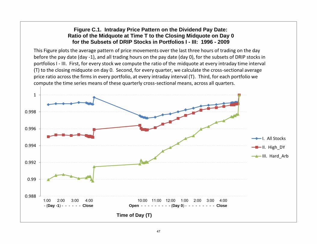
0.988

0.99

0.992

0.994

0.996

0.998

1

I. All Stocks

II. High_DY

III. Hard_Arb

1:00 2:00 3:00 4:00 10:00 11:00 12:00 1:00 2:00 3:00 4:00

- (Day -1) - - - - - - Close Open - - - - - - - - - (Day 0) - - - - - - - - - Close

Time of Day (T)

Figure C.1. Intraday Price Pattern on the Dividend Pay Date: Ratio of the Midquote at Time T to the Closing Midquote on Day 0 for the Subsets of DRIP Stocks in Portfolios I - III: 1996 - 2009

This Figure plots the average pattern of price movements over the last three hours of trading on the day before the pay date (day -1), and all trading hours on the pay date (day 0), for the subsets of DRIP stocks in portfolios I - III. First, for every stock we compute the ratio of the midquote at every intraday time interval (T) to the closing midquote on day 0. Second, for every quarter, we calculate the cross-sectional average price ratio across the firms in every portfolio, at every intraday interval (T). Third, for each portfolio we compute the time series means of these quarterly cross-sectional means, across all quarters.

47

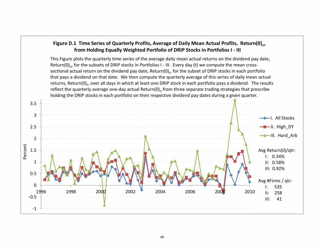
-1

-0.5

0

0.5

1

1.5

2

2.5

3

3.5

1996 1998 2000 2002 2004 2006 2008 2010

Per

cen

t

I. All Stocks

II. High_DY

III. Hard_Arb

Figure D.1 Time Series of Quarterly Profits, Average of Daily Mean Actual Profits, Return(0)n, from Holding Equally Weighted Portfolio of DRIP Stocks in Portfolios I - III

This Figure plots the quarterly time series of the average daily mean actual returns on the dividend pay date, Return(0)n, for the subsets of DRIP stocks in Portfolios I - III. Every day (t) we compute the mean cross- sectional actual return on the dividend pay date, Return(0)t, for the subset of DRIP stocks in each portfolio that pays a dividend on that date. We then compute the quarterly average of this series of daily mean actual returns, Return(0)t, over all days in which at least one DRIP stock in each portfolio pays a dividend. The results reflect the quarterly average one-day actual Return(0)n from three separate trading strategies that prescribe holding the DRIP stocks in each portfolio on their respective dividend pay dates during a given quarter.

Avg Return(0)/qtr: I: 0.34% II: 0.58% III: 0.92% Avg #Firms / qtr: I: 535 II: 258 III: 41

48

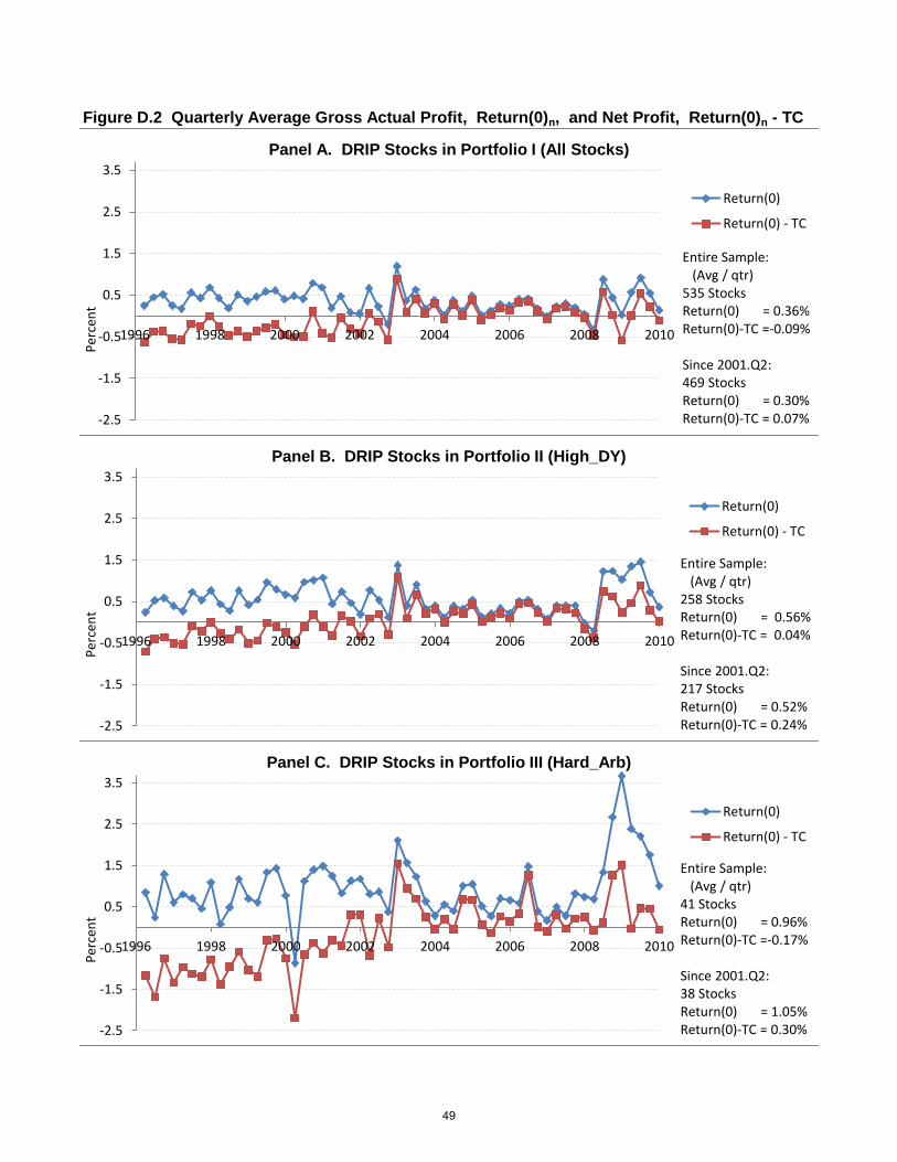
Figure D.2 Quarterly Average Gross Actual Profit, Return(0)n, and Net Profit, Return(0)n - TC

7985

7986

7987

7988

7989

7990

7991

7992

7993

7994

7995

7996

7997

7998

7999

8000

8001

8002

8003

8004

8005

8006

8007

8008

8009

8010

8011

8012

-2.5

-1.5

-0.5

0.5

1.5

2.5

3.5

1996 1998 2000 2002 2004 2006 2008 2010

Per

cen

t

Panel A. DRIP Stocks in Portfolio I (All Stocks)

Return(0)

Return(0) - TC

Entire Sample: (Avg / qtr) 535 Stocks Return(0) = 0.36% Return(0)-TC =-0.09% Since 2001.Q2: 469 Stocks Return(0) = 0.30% Return(0)-TC = 0.07%

-2.5

-1.5

-0.5

0.5

1.5

2.5

3.5

1996 1998 2000 2002 2004 2006 2008 2010

Per

cen

t

Panel B. DRIP Stocks in Portfolio II (High_DY)

Return(0)

Return(0) - TC

Entire Sample: (Avg / qtr) 258 Stocks Return(0) = 0.56% Return(0)-TC = 0.04% Since 2001.Q2: 217 Stocks Return(0) = 0.52% Return(0)-TC = 0.24%

-2.5

-1.5

-0.5

0.5

1.5

2.5

3.5

1996 1998 2000 2002 2004 2006 2008 2010

Per

cen

t

Panel C. DRIP Stocks in Portfolio III (Hard_Arb)

Return(0)

Return(0) - TC

Entire Sample: (Avg / qtr) 41 Stocks Return(0) = 0.96% Return(0)-TC =-0.17% Since 2001.Q2: 38 Stocks Return(0) = 1.05% Return(0)-TC = 0.30%

49

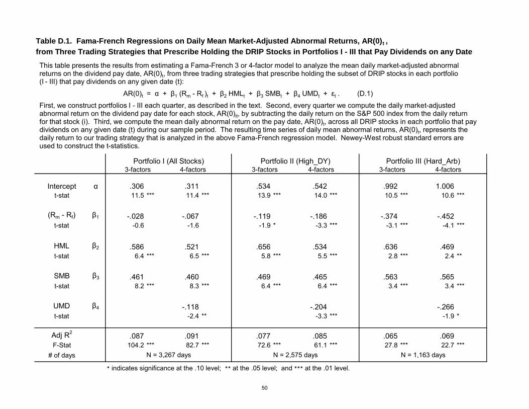
Table D.1. Fama-French Regressions on Daily Mean Market-Adjusted Abnormal Returns, AR(0)t ,

from Three Trading Strategies that Prescribe Holding the DRIP Stocks in Portfolios I - III that Pay Dividends on any Date

Intercept α .306 .311 .534 .542 .992 1.006

t-stat 11.5 *** 11.4 *** 13.9 *** 14.0 *** 10.5 *** 10.6 ***

(Rm - Rf) β1 -.028 -.067 -.119 -.186 -.374 -.452

t-stat -0.6 -1.6 -1.9 * -3.3 *** -3.1 *** -4.1 ***

HML β2 .586 .521 .656 .534 .636 .469

t-stat 6.4 *** 6.5 *** 5.8 *** 5.5 *** 2.8 *** 2.4 **

SMB β3 .461 .460 .469 .465 .563 .565

t-stat 8.2 *** 8.3 *** 6.4 *** 6.4 *** 3.4 *** 3.4 ***

UMD β4 -.118 -.204 -.266

t-stat -2.4 ** -3.3 *** -1.9 *

Adj R2

.087 .091 .077 .085 .065 .069

F-Stat 104.2 *** 82.7 *** 72.6 *** 61.1 *** 27.8 *** 22.7 ***

# of days

* indicates significance at the .10 level; ** at the .05 level; and *** at the .01 level.

N = 3,267 days N = 2,575 days N = 1,163 days

Portfolio I (All Stocks) Portfolio II (High_DY) Portfolio III (Hard_Arb)3-factors 4-factors 3-factors 4-factors 3-factors 4-factors

This table presents the results from estimating a Fama-French 3 or 4-factor model to analyze the mean daily market-adjusted abnormal returns on the dividend pay date, AR(0)t, from three trading strategies that prescribe holding the subset of DRIP stocks in each portfolio (I - III) that pay dividends on any given date (t):

AR(0)t = α + β1 (Rm - Rf )t + β2 HMLt + β3 SMBt + β4 UMDt + ɛt . (D.1)

First, we construct portfolios I - III each quarter, as described in the text. Second, every quarter we compute the daily market-adjusted abnormal return on the dividend pay date for each stock, AR(0)it, by subtracting the daily return on the S&P 500 index from the daily return for that stock (i). Third, we compute the mean daily abnormal return on the pay date, AR(0)t, across all DRIP stocks in each portfolio that pay dividends on any given date (t) during our sample period. The resulting time series of daily mean abnormal returns, AR(0)t, represents the daily return to our trading strategy that is analyzed in the above Fama-French regression model. Newey-West robust standard errors are used to construct the t-statistics.

50