downscaling regional climate data to calculate the ... · pdf filenyman et al.: downscaling...

Australian Meteorological and Oceanographic Journal 64 (2014) 109–122

109

Downscaling regional climate data to calculate the radiative index of dryness

in complex terrain

Petter Nyman1,2, Christopher B.Sherwin1,3, Christoph Langhans1, Patrick N.J. Lane1,2 and Gary J. Sheridan1,2

1Department of Forest and Ecosystem Science, The University of Melbourne, Victoria, Australia

2Bushfire Cooperative Research Centre, Victoria, Australia3Esri Australia, Victoria, Australia

(Manuscript received November 2013, revised May 2014)

The radiative index of dryness (or aridity index) is a non-dimensional measure of the long-term balance between rainfall and net radiation. Quantifying aridity re-quires spatially distributed information on net radiation and rainfall. The variabil-ity in net radiation in complex terrain can be modelled at high spatial resolution by combining point data with equations that incorporate the effects of elevation, surface geometry and atmospheric attenuation of incoming radiation. At large spatial scales and over long time periods, however, the combination of seasonal-ity, year to year variations and spatial variability in climate result in complex spa-tial-temporal patterns of incoming radiation, which are more effectively captured in satellite-based measurements. This study uses a high resolution model of short-wave radiation as a tool for downscaling satellite-derived data on incoming radia-tion. The aim was to incorporate topographic effects on net radiation in complex terrain while retaining information on regional and seasonal trends captured in satellite data. The method relies on satellite-based measures of incoming radiation from the Australian Bureau of Meteorology (BoM) to provide the spatial cover-age and long-term data that represent the average incoming radiation across the state of Victoria in southeast Australia. These long-term data were coupled with a topographic downscaling algorithm to produce estimates of net radiation and aridity at the resolution of a 20 m digital elevation model. Results show that annual precipitation (and cloud fraction) gradients drive the variability in aridity at large scales (10–100 km) while topography (e.g. slope aspect and slope angle) are the main drivers at small scales (e.g. 1 km). The aridity index varied between 0.24 and 10.95 across the state of Victoria. The effect of aridity on vegetation was apparent at local scales through systematic variations in tree-height along rainfall gradients and across aspects with different levels of exposure to solar radiation.

Introduction

Landscape aridity can be calculated from the annual sum of net radiation (Rn) and precipitation (P) through the ratio

Rn/λP, where λ is the latent heat of vaporisation. This ratio is the radiative index of dryness, AIB (Budyko 1974), which can be used alongside measures of Rn to examine the effects of water and energy availability on vegetation, soil and water dynamics (e.g. Berry et al. 2006). Net radiation (Rn) is the energy balance at the earth surface and is a function of short- and longwave radiation fluxes. At large scales, the variability in these fluxes is caused by latitude,

Corresponding author address: Petter Nyman, Department of Forest and Ecosystem Science, The University of Melbourne, 221 Bouverie St, Parkville, Victoria, 3010, Australia. Email: [email protected]

110 Australian Meteorological and Oceanographic Journal 64:2 June 2014

is highly variable. Large-scale and long-term patterns in radiation fluxes are more effectively measured from geostationary satellites, which provide continental-scale data at high temporal resolution (minutes to hours). With these measurements the spatial distribution of incoming radiation can be characterised over time for large areas, while incorporating the seasonal and year to year variability caused by temporal and spatial changes in atmospheric conditions due to latitude, cloud cover, smoke and dust (Gupta et al. 1999; Ridley et al. 2010; Weymouth and Le Marshall 2001). The accuracy of satellite derived measures can easily be evaluated at different points in the landscape using ground based measurements of incoming radiation (Weymouth and Le Marshall 2001).

In regional-scale studies of soil and water processes the AIB can be quantified using data on broad-scale patterns in rainfall and radiation fluxes (Berry et al. 2006; Berry and Roderick 2004). In regions with complex terrain however, the localised variation in water and energy availability can be large, and an explicit representation of landscape heterogeneity may be needed in order to model landscape processes (Donohue et al. 2012; Istanbulluoglu et al. 2008). However, the methods for representing heterogeneity in net radiation and aridity to date have focused either on the modelling of topographic effects on net radiation at a high spatial resolution within relatively small catchments (< 100 m2) (Wilson and Gallant 2000, Moore et al. 1993), or on the quantification of regional-scale variation in incoming radiation using satellite data (Boland et al. 2008; Weymouth and Le Marshall 2001).

This study presents a method for downscaling satellite derived data on incoming radiation in order to quantify long-term average values of net radiation and aridity at high spatial resolution over a large area containing complex terrain. Satellite-derived measures of incoming radiation from the Australian Bureau of Meteorology (BoM) provided broad spatial coverage and long-term radiation data at coarse resolution (5 km) across Australia. This data was coupled with models of topographic effects on net radiation to produce a high resolution (20 m) measure of aridity that retained important information on the regional and seasonal trends captured in the regional and long-term data from BoM. The two specific objectives of the study were to:1. Calculate topographic effects on shortwave radiation

using satellite-derived measures of radiation to partition incoming radiation into diffuse and direct components.

2. Combine long-term satellite data with a model of topographic effects and spatially interpolated rainfall to calculate the radiative index of dryness (AIB) at 20 m resolution across a large region.The paper first describes the method for calculating net

radiation and aridity at high spatial resolution, using data and theoretical models of short- and longwave radiation fluxes. As an example of model application, the calculations were then carried out using a 20 m digital elevation model for Victoria in southeast Australia. The region has variable

surface albedo, elevation, atmospheric composition and cloud cover (Budyko 1974; Ohring and Clapp 1980; Ohta et al. 1993). At local scales, the variability is driven primarily by topographic effects, but also heterogeneity in surface albedo and emissivity (Moore et al. 1993; Nunez 1980). Precipitation (P) varies at large scales with global circulation patterns and regional climatology (Rasmusson and Arkin 1993), whereas at local scale, the variability in P is caused by prevailing weather patterns and orographic effects (Adam et al. 2006; Hutchinson 1998). The combination of regional and local variability in P and Rn means that energy and water availability is dominated by different variables at different scales. At small scales the topography and local climatology leads to heterogeneous (or patchy) patterns of variability (Band 1993; Moore et al. 1993; Tajchman and Lacey 1986) while factors such as latitude and global circulation patterns lead to gradients of variability at regional and global scales (Running et al. 2000).

Patterns in water and energy availability can be determined for large scales using a combination of i) satellite data, ii) modelling of surface-atmosphere interactions, and iii) spatial interpolation of point based data (Berry and Roderick 2004; Nemani et al. 2003). In complex terrain, these approaches underestimate the small-scale variability introduced by orographic and topographic effects on Rn and P. Orographic variation in precipitation can be captured to some extent by accounting for the systematic changes in precipitation with elevation (e.g. Hutchinson 1998). For net radiation, the topographic effects are more complex due to the strong dependency on multiple factors including elevation, slope orientation (slope and aspect), shading and the proportion of diffuse radiation. At mid- to high latitudes, the slope orientation can have large effects on Rn with implications for water and energy availability at small scales (Moore et al. 1993). The resulting heterogeneity in ecological, hydrological and geomorphic processes at these small scales can be important sources of uncertainty when modelling catchment processes (Badano et al. 2005; Band 1993; Bradstock et al. 2010; Holland and Steyn 1975; Holst et al. 2005; Nunez 1980).

Net radiation in complex terrain can be modelled by combining point data from weather stations with equations that incorporate the effects of elevation, surface geometry and atmospheric attenuation of incoming radiation (Moore et al. 1993; Running et al. 1987; Wilson and Gallant 2000). This modelling approach is effective at capturing small scale topographic effects on incoming radiation and temperature. Using point based data and a topographic model to model the average long-term radiation at regional scales is problematic, however, when the distribution of weather stations is sparse and the spatial-temporal variations in atmospheric conditions are high. Large uncertainties can be introduced by spatially interpolating point-based climate data to represent the effects of clouds on the partitioning of incoming radiation into diffuse and direct proportions, particularly in mountainous terrain where cloudiness

Nyman et al.: Downscaling regional climate data to calculate the radiative index of dryness in complex terrain 111

Eqn. 2 is negligible. Precipitation was obtained from monthly precipitation grids (2.5 km resolution) from the Australian Bureau of Meteorology which had been interpolated using a 3-D spline surface fitting algorithm (Xu and Hutchinson 2011) (Table 1). Monthly daily temperature in each month,TD, was modelled at 20 m resolution using the method described later in section 2.3.

Net radiation (Rn) is the balance of shortwave radiation and the downward and upward longwave radiation fluxes:

Rn= Rs+ Rld- Rlu

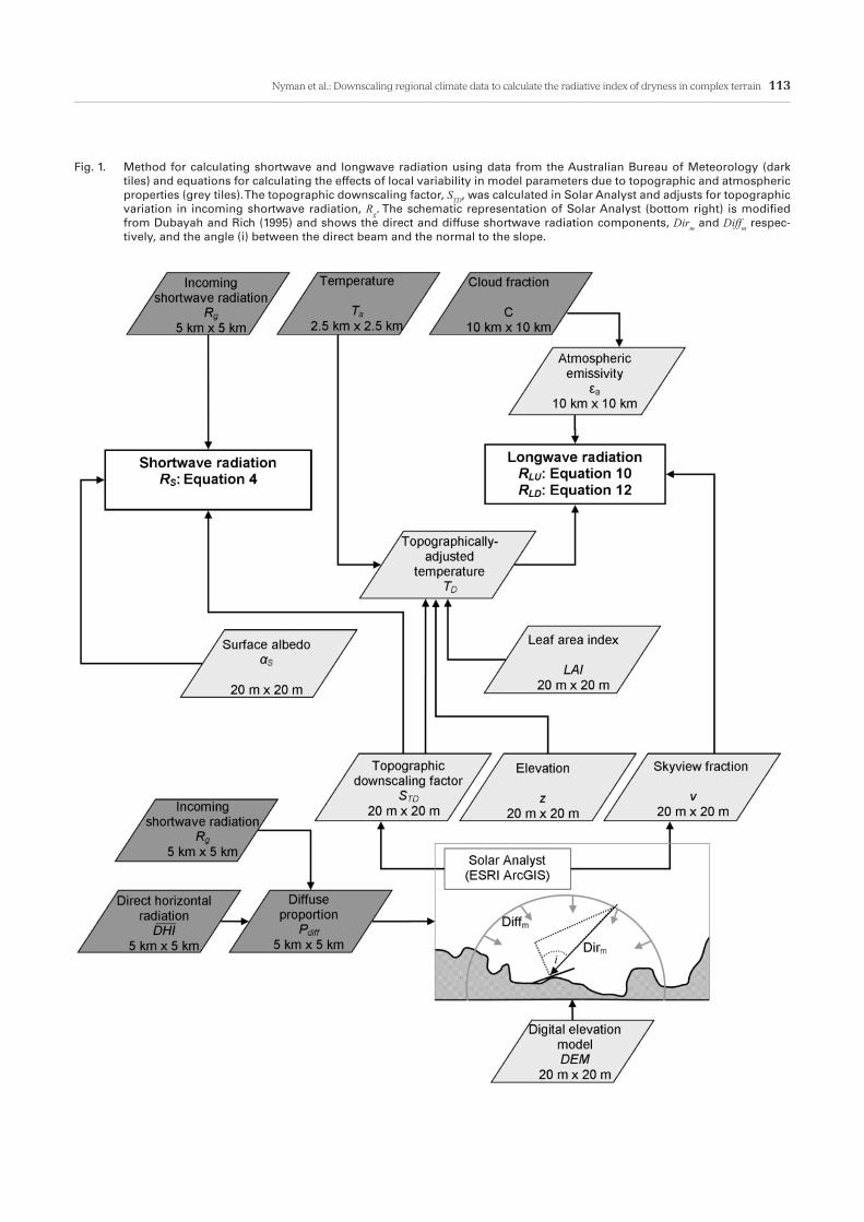
where Rs is the net shortwave radiation (MJ m-2 day-1), Rld (MJ m-2 day-1) is the incoming longwave radiation, and Rlu (MJ m-2 day-1) is the upward longwave radiation. All radiation fluxes are given as daily values averaged for each month. Methods for calculating short- and longwave radiation are described below and shown schematically in Fig. 1.

Shortwave radiationThe daily net shortwave radiation (Rs) averaged for each month was calculated at 20 m resolution from the global incoming shortwave radiation (Rg), the topographic downscaling factor (STD) and the surface albedo (αs):

Rs=(1-αs ) Rg STD

The global incoming shortwave radiation (Rg) is the long-term daily incoming shortwave radiation at 5 km x 5 km grid resolution averaged for each month. It was calculated from instantaneous global horizontal irradiance, GHI (W m-2), from the Australian Bureau of Meteorology which uses imagery from geostationary meteorological satellites (JMA and NOAA) (Weymouth and Le Marshall 2001; Table 1). Hourly irradiance data from 01 January 1990 to 30 June 2012 was aggregated to produce the long-term average daily Rg for each month.

...(3)

...(4)

climate, strong rainfall gradients and areas with complex terrain, and therefore provides an opportunity to explore the effects of climatic and topographic parameters on net radiation and aridity at different scales. Spatial variations in aridity are likely to affect soil, vegetation structure and the overall forest productivity across the landscape. The study therefore includes an exploratory analysis of variation in tree height in order to determine whether forests respond to small scale variation in AIB. Tree height was considered a suitable variable for exploring the environmental effects of AIB because (i) it is related to forest productivity and strongly influenced by water availability (Eamus 2003; Niklas 2007) and (ii) it can be measured using airborne lidar at a resolution and scale which corresponds to the AIB calculations (Nilsson, 1996).

Methods

Defining aridity and net radiation Aridity (or the Budyko radiative index of dryness), AIB, was calculated for each month of the year as the ratio of the average daily net radiation, Rn (MJ m-2 day-1), to the energy required to evaporate the average daily rainfall in that month, λP (Budyko 1958),

where P is the average daily rainfall (m day-1) in each month and λ is the latent heat of evaporation (MJ m-3) which is a function of mean daily temperature, TD (K) (Harrison 1963):

For temperatures ranging from 278.15 K (5 °C) to 303.15 K (30 °C) the latent heat of evaporation λ varies between 2490 and 2430 MJ m-3 which (given the other sources of uncertainty) effectively means that the temperature effect in

...(1)

...(2)

Table 1. Spatial datasets from the Australian Bureau of Meteorology.

Parameter Data Description Resolution and duration of the recorda

Solar global horizontal irradiance (GHI)

GHI is the instantaneous intensity (W m-2) of solar energy falling on a horizontal surface and is derived from hourly satellite data.

Spatial resolution of 0.05 degrees in latitude and longitude (~ 5.0 km). Hourly measurements from January 1990 to 30 June 2012.

Solar direct normal irradiance (DNI)

DNI is the instantaneous intensity (W m-2) of solar direct beam energy falling on a surface normal to the beam.

Spatial resolution of 0.05 degrees in latitude and longitude (~ 5.0 km). Hourly measurements from January 1990 to 30 June 2012.

Temperature (T1)Mean monthly temperature (K) interpolated using 3-D spline surface fitting algorithm (Xu and Hutchinson 2011).

Spatial resolution of 0.025 degrees (~2.5 km) Average values produced using data records extending from 1911 to June 2011.

Precipitation (P)Mean monthly precipitation (mm) interpolated using 3-D Spline (surface fitting algorithm) (Xu and Hutchinson 2011).

Spatial resolution of 0.025 degrees (~ 2.5 km). Produced from a 30-year rainfall period from 1961 to 1990.

Cloud fraction (C)

Mean monthly cloud fraction interpolated using 3-D spline surface fitting algorithm (Xu and Hutchinson 2011). Average daily values in each month were obtained from measurement made at 9.00 am and 3.00 pm.

Spatial resolution of 0.1 degrees (~ 10 km). Produced from a 30-year measurement period from 1976 to 2005.

1 More information on datasets is available at: www.bom.gov.au/climate/averages/climatology/gridded-data-info/gridded_datasets_summary.shtml

http://www.bom.gov.au/climate/averages/climatology/gridded-data-info/gridded_datasets_summary.shtml

http://www.bom.gov.au/climate/averages/climatology/gridded-data-info/gridded_datasets_summary.shtml


The annual average αs was assigned values based on leaf area index (LAI) of four broad vegetation categories in Victoria (southeast Australia) distinguished based on ecological vegetation class (EVC), which is a classification scheme developed by the Victorian Department of Environment and Primary Industries (2011). The EVCs were grouped into three broad categories of wet, damp and dry forest which were assigned LAI values of four, three and two, respectively, based on the range of values reported for different forest types in southeast Australia (Hill et al. 2006; Pierce et al. 1993). Non-forested areas (mainly comprising grasslands and agricultural areas) were assigned an LAI of 1. The LAI was used to calculate αs based on the relation described in Hales et al. (2004):

αs=0.3352 – 0.1827(1 – e–1.3LAI)

Values of αs were 0.15 for wet forests, 0.16 for damp forests, 0.17 for dry forests and 0.20 for all other land surfaces.

When the earth surface is flat the Rs in Eqn.4 is equal to (1-αs)Rg, while in complex terrain Rs may be higher or lower than (1–αs)Rg depending on topography. The topographic downscaling factor, STD, in Eqn.4 adjusts for the effects of variable slope angle, aspect and shading. It was calculated at 20 m resolution using Solar Analyst (ESRI), which couples information on the position of the sun with a DEM to model effects of shading and slope orientation on Rs (Fu and Rich 2002). The algorithms in Solar Analyst generate upward-looking viewsheds based on the DEM and models incoming direct (Dirm) and diffuse (Diffm) shortwave radiation separately from each sky direction for a given sun position. Calculations of Dirm and Diffm were performed at hourly time steps and output as daily values averaged for each month. Due to the large study area of Victoria (227416 km2), the 5 x 5 km grids in the irradiance data from BoM were used as a tile template for data processing with latitude being the mid-point of each tile. A buffer of 1.5 km was added to each tile to eliminate edge effects by ensuring that the effects of topographic shading from outside each five km tile were retained in the modelled shortwave radiation.

The topographic downscaling factor, STD, was obtained by normalising the modelled shortwave radiation (Dirm + Diffm) at each 20 m cell in the DEM by Rtile, which is the spatially average incoming shortwave radiation modelled for the entire 5 x 5 km tile:

The topographic downscaling matrix, STD, is the incoming shortwave radiation on a 20 m pixel relative to the average (or global) incoming shortwave radiation across the 5 x 5 km tile.

The diffuse proportion of the shortwave radiation (Pdiff) is mainly non-directional and is input to Solar Analyst before calculating Dirm and Diffm. The long-term average Pdiff was obtained for each 5 x 5 km tile using irradiance data from BoM. First, the direct irradiance on a horizontal surface, DHI (W m-2), was calculated from the normal irradiance, DNI (W m-2) (Table 1) by correcting for zenith angle of the sun (m):

...(5)

...(6)

DHI=DNI cos m

The DHI was calculated for each hour of the year after averaging the hourly DNI data from 1990–2012 into a single year. The hourly values of DNI and DHI were then summed into daily totals and averaged for each month, producing DNI and DHI (in MJ m-2 day-1), respectively. Daily diffuse radiation in each month falling on a horizontal surface, Rdiff (MJ m-2 day-1) was then calculated from Rg and DHI:

Rdiff = Rg – DHI

The monthly diffuse proportion (Pdiff) at 5 km resolution is then:

Pdiff varies spatially and seasonally depending on variation in cloud cover and sun position.

Longwave radiationUpward longwave radiation, Rlu (MJ m-2 day-1) was calculated from:

where εs is the surface emissivity (0.96 in forests) (Brutsaert 2005), σ is the Stefan-Boltzmann constant (MJ m-2 K-4 day-1) and TD is the topographically adjusted surface temperature. Long-term average surface temperature is unknown across the Victorian region and TD is therefore assumed to represent both surface and air temperature. Topographically adjusted temperature TD was obtained by combining regionally interpolated monthly average air temperature (Ta) from BoM (Table 1) with an equation from SRAD (Moore et al. 1993) that adjusts for local variations in incoming radiation STD, elevation (z) and leaf area index (LAI):

where Tlapse (K 1000 m-1) is the change in temperature with elevation, zb is the average elevation (m) within each tile, LAImax is the maximum LAI within each tile, and k is a constant (set to 1). In the southern hemisphere, Eqn.11 increases temperatures on north-facing slopes and decreases temperature on south-facing slopes relative to a flat surface (Moore et al. 1993).

Downward longwave radiation, Rld (MJ m-2 day-1) was calculated from:

where v is the sky-view fraction, and εa is the atmospheric emissivity which was calculated based on the equation developed by Swinbank (1963) and modified by Crawford and Duchon (1999) to include the effects of cloud cover:

where C is the monthly cloud fraction (Table 1). Emissivity varies from 1 for 100 per cent cloud (in which case it is not a

...(7)

...(8)

...(9)

...(10)

...(11)

...(12)

...(13)


Fig. 1. Method for calculating shortwave and longwave radiation using data from the Australian Bureau of Meteorology (dark tiles) and equations for calculating the effects of local variability in model parameters due to topographic and atmospheric properties (grey tiles). The topographic downscaling factor, STD, was calculated in Solar Analyst and adjusts for topographic variation in incoming shortwave radiation, Rg. The schematic representation of Solar Analyst (bottom right) is modified from Dubayah and Rich (1995) and shows the direct and diffuse shortwave radiation components, Dirm and Diffm respec-tively, and the angle (i) between the direct beam and the normal to the slope.


function of temperature), to a function of temperature only, when there is no cloud.

The sky-view fraction, v, is the fraction of visible sky at a point on the earth surface, ranging from 1 (unobstructed) to 0 (completely obstructed). It was quantified statistically from a DEM in a sample of 20 tiles (5 km x 5 km) in the Victorian uplands. The analysis focused on upland areas because it is where topographic effects on v are likely to operate. The sky-view, v (-), the local slope, GS (°), the difference between lowest and highest point (i.e. the relief) in each tile, IR (m), and the elevation of each point, GD (m), were obtained from ArcGIS at 50 random points (20 m x 20 m) within each tile (1000 grid points in total). The following relation was obtained for v:

v= βI + βSGS + βRIR + βDGD , 0 ≤ v ≤ 1

where βI is the intercept (equal to 1), βS is the slope coefficient (-6.65 x 10-3), βR is the relief coefficient (-1.45 x 10-4) and βD is the elevation coefficient (5.60 x 10-5) (F3, 995 = 1290, p<<0.01, R2 = 0.8) . The dimensions of the coefficients are such that v remains non-dimensional.

Results

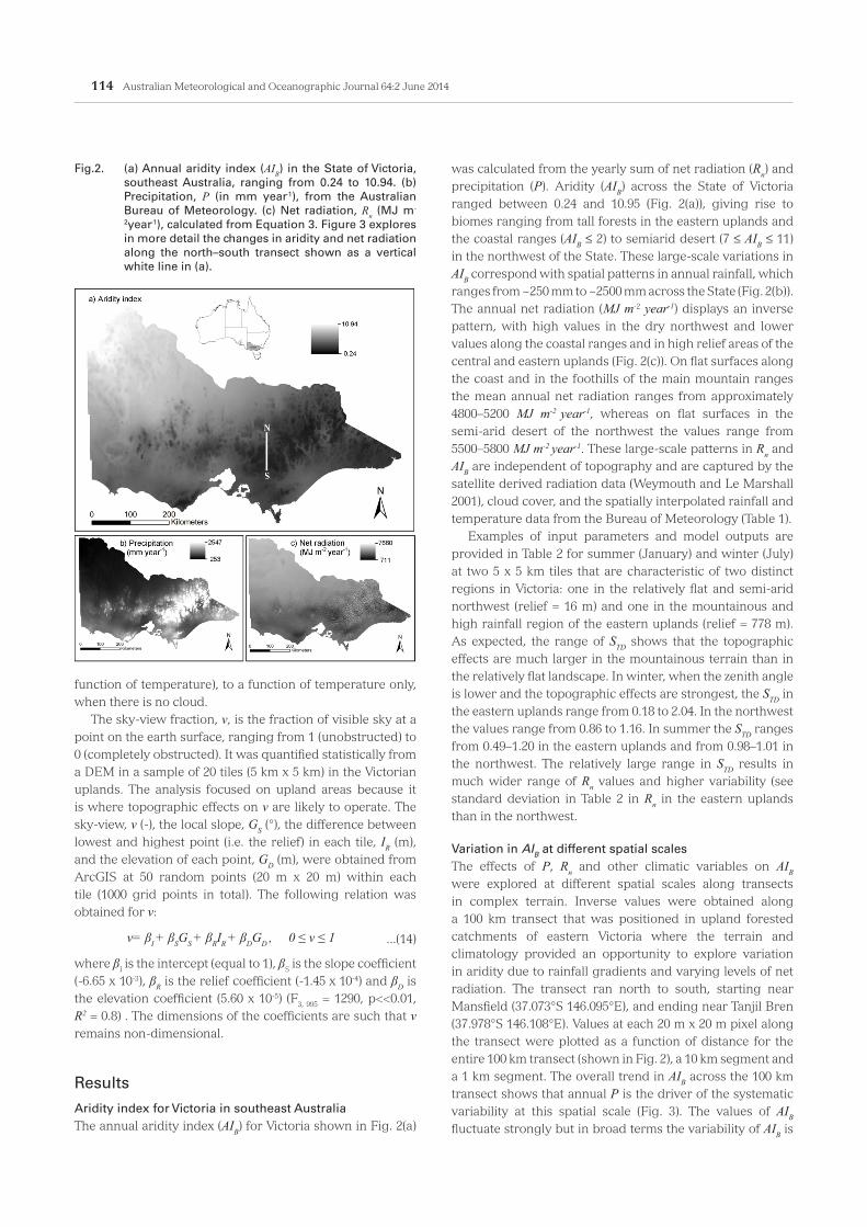
Aridity index for Victoria in southeast AustraliaThe annual aridity index (AIB) for Victoria shown in Fig. 2(a)

...(14)

was calculated from the yearly sum of net radiation (Rn) and precipitation (P). Aridity (AIB) across the State of Victoria ranged between 0.24 and 10.95 (Fig. 2(a)), giving rise to biomes ranging from tall forests in the eastern uplands and the coastal ranges (AIB ≤ 2) to semiarid desert (7 ≤ AIB ≤ 11) in the northwest of the State. These large-scale variations in AIB correspond with spatial patterns in annual rainfall, which ranges from ~250 mm to ~2500 mm across the State (Fig. 2(b)). The annual net radiation (MJ m-2 year-1) displays an inverse pattern, with high values in the dry northwest and lower values along the coastal ranges and in high relief areas of the central and eastern uplands (Fig. 2(c)). On flat surfaces along the coast and in the foothills of the main mountain ranges the mean annual net radiation ranges from approximately 4800–5200 MJ m-2 year-1, whereas on flat surfaces in the semi-arid desert of the northwest the values range from 5500–5800 MJ m-2 year-1. These large-scale patterns in Rn and AIB are independent of topography and are captured by the satellite derived radiation data (Weymouth and Le Marshall 2001), cloud cover, and the spatially interpolated rainfall and temperature data from the Bureau of Meteorology (Table 1).

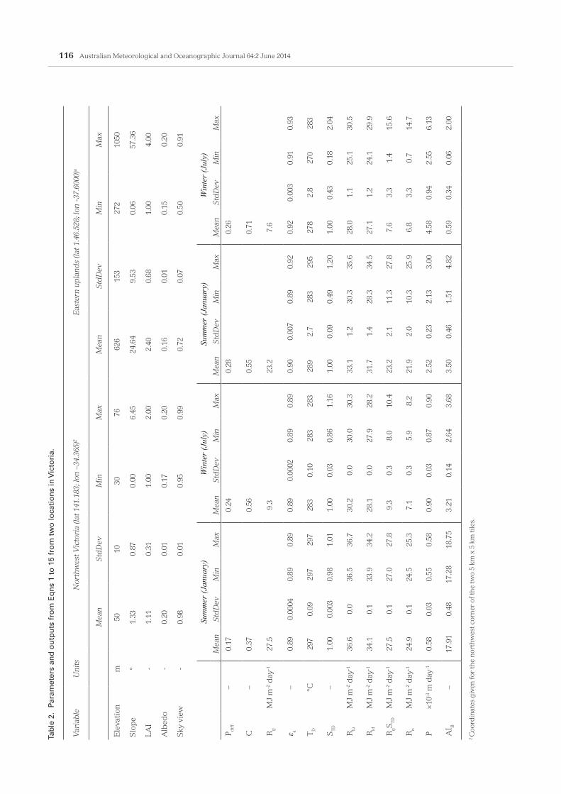
Examples of input parameters and model outputs are provided in Table 2 for summer (January) and winter (July) at two 5 x 5 km tiles that are characteristic of two distinct regions in Victoria: one in the relatively flat and semi-arid northwest (relief = 16 m) and one in the mountainous and high rainfall region of the eastern uplands (relief = 778 m). As expected, the range of STD shows that the topographic effects are much larger in the mountainous terrain than in the relatively flat landscape. In winter, when the zenith angle is lower and the topographic effects are strongest, the STD in the eastern uplands range from 0.18 to 2.04. In the northwest the values range from 0.86 to 1.16. In summer the STD ranges from 0.49–1.20 in the eastern uplands and from 0.98–1.01 in the northwest. The relatively large range in STD results in much wider range of Rn values and higher variability (see standard deviation in Table 2 in Rn in the eastern uplands than in the northwest.

Variation in AIB at different spatial scalesThe effects of P, Rn and other climatic variables on AIB were explored at different spatial scales along transects in complex terrain. Inverse values were obtained along a 100 km transect that was positioned in upland forested catchments of eastern Victoria where the terrain and climatology provided an opportunity to explore variation in aridity due to rainfall gradients and varying levels of net radiation. The transect ran north to south, starting near Mansfield (37.073°S 146.095°E), and ending near Tanjil Bren (37.978°S 146.108°E). Values at each 20 m x 20 m pixel along the transect were plotted as a function of distance for the entire 100 km transect (shown in Fig. 2), a 10 km segment and a 1 km segment. The overall trend in AIB across the 100 km transect shows that annual P is the driver of the systematic variability at this spatial scale (Fig. 3). The values of AIB fluctuate strongly but in broad terms the variability of AIB is

Fig.2. (a) Annual aridity index (AIB) in the State of Victoria, southeast Australia, ranging from 0.24 to 10.94. (b) Precipitation, P (in mm year-1), from the Australian Bureau of Meteorology. (c) Net radiation, Rn (MJ m-

2year-1), calculated from Equation 3. Figure 3 explores in more detail the changes in aridity and net radiation along the north–south transect shown as a vertical white line in (a).


inversely related to the precipitation. A peak in precipitation of ~1800 mm corresponds with the minimum AIB. Systematic changes in precipitation are related to elevation and are a function of the 3-D spine interpolation used to create the 2.5 km rainfall grid from point data (Xu and Hutchinson 2011).

Fluctuations in aridity at small scales within the 100 km transect are almost as large as the average change in aridity caused by increasing the rainfall from 900 mm to 1800 mm. The one km segment of the transect shows that

these fluctuations are independent of rainfall. Instead they are caused by variation in net radiation, Rn, which fluctuates (at high spatial resolution) between 6000 and 2000 MJ m-2 year-1 around a mean value of ~4000 MJ m-2year-1. This small-scale variation in Rn is caused by aspect-dependent changes in the downscaled incoming shortwave radiation (RgSTD). At the intermediate scale (10 km), both P and Rn influence on AIB. The change in aspect from north to south causes a small drop in AIB as a result of reduced Rn, but the reduction is

Fig. 3. North to south transect at three scales (100 km, 10 km and 1 km) showing elevation (z), precipitation (P), and downscaled values of aridity index (AIB), annual net radiation (Rn) and incoming shortwave radiation (RgSTD). The 0–100 km transect is shown in Fig. 2.

116 Australian Meteorological and Oceanographic Journal 64:2 June 2014Ta

ble

2.

Para

met

ers

and

ou

tpu

ts f

rom

Eq

ns

1 to

15

fro

m t

wo

loca

tio

ns

in V

icto

ria.

Var

iabl

eU

nits

Nor

thw

est V

icto

ria

(lat 1

41.1

83; l

on –

34.3

65)2

Eas

tern

upl

ands

(lat

1.4

6.52

8; lo

n -3

7.60

00)a

Mea

nSt

dDev

Min

Max

Mea

nSt

dDev

Min

Max

Ele

vati

onm

5010

3076

626

153

272

1050

Slo

pe

°1.

330.

870.

006.

4524

.64

9.53

0.06

57.3

6

LA

I-

1.11

0.31

1.00

2.00

2.40

0.68

1.00

4.00

Alb

edo

-0.

200.

010.

170.

200.

160.

010.

150.

20

Sky

vie

w-

0.98

0.01

0.95

0.99

0.72

0.07

0.50

0.91

Sum

mer

(Jan

uary

)W

inte

r (Ju

ly)

Sum

mer

(Jan

uary

)W

inte

r (Ju

ly)

Mea

nSt

dDev

Min

Max

Mea

nSt

dDev

Min

Max

Mea

nSt

dDev

Min

Max

Mea

nSt

dDev

Min

Max

P dif

f–

0.17

0.24

0.28

0.26

C

–0.

370.

560.

550.

71

Rg

MJ

m-2 d

ay-1

27.5

9.3

23.2

7.6

ε a–

0.89

0.00

040.

890.

890.

890.

0002

0.89

0.89

0.90

0.00

70.

890.

920.

920.

003

0.91

0.93

T D°C

297

0.09

297

297

283

0.10

283

283

289

2.7

283

295

278

2.8

270

283

STD

–1.

000.

003

0.98

1.01

1.00

0.03

0.86

1.16

1.00

0.09

0.49

1.20

1.00

0.43

0.18

2.04

Rlu

MJ

m-2 d

ay-1

36.6

0.0

36.5

36.7

30.2

0.0

30.0

30.3

33.1

1.2

30.3

35.6

28.0

1.1

25.1

30.5

Rld

MJ

m-2 d

ay-1

34.1

0.1

33.9

34.2

28.1

0.0

27.9

28.2

31.7

1.4

28.3

34.5

27.1

1.2

24.1

29.9

RgS

TDM

J m

-2 d

ay-1

27.5

0.1

27.0

27.8

9.3

0.3

8.0

10.4

23.2

2.1

11.3

27.8

7.6

3.3

1.4

15.6

Rn

MJ

m-2 d

ay-1

24.9

0.1

24.5

25.3

7.1

0.3

5.9

8.2

21.9

2.0

10.3

25.9

6.8

3.3

0.7

14.7

P×

10-3 m

day

-10.

580.

030.

550.

580.

900.

030.

870.

902.

520.

232.

133.

004.

580.

942.

556.

13

AI B

–17

.91

0.48

17.2

818

.75

3.21

0.14

2.64

3.68

3.50

0.46

1.51

4.82

0.59

0.34

0.06

2.00

2 C

oord

inat

es g

iven

for

the

nor

thw

est c

orn

er o

f th

e tw

o 5

km x

5 k

m ti

les.


negated by the simultaneous effects of reduction in rainfall.

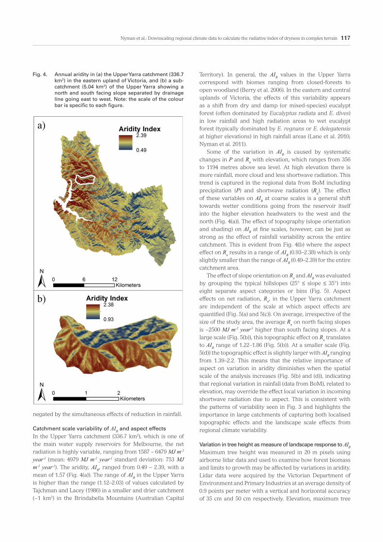
Catchment scale variability of AIB and aspect effectsIn the Upper Yarra catchment (336.7 km2), which is one of the main water supply reservoirs for Melbourne, the net radiation is highly variable, ranging from 1587 – 6479 MJ m-2 year-1 (mean: 4979 MJ m-2 year-1 standard deviation: 753 MJ m-2 year-1). The aridity, AIB, ranged from 0.49 – 2.39, with a mean of 1.57 (Fig. 4(a)). The range of AIB in the Upper Yarra is higher than the range (1.12–2.03) of values calculated by Tajchman and Lacey (1986) in a smaller and drier catchment (~1 km2) in the Brindabella Mountains (Australian Capital

Territory). In general, the AIB values in the Upper Yarra correspond with biomes ranging from closed-forests to open woodland (Berry et al. 2006). In the eastern and central uplands of Victoria, the effects of this variability appears as a shift from dry and damp (or mixed-species) eucalypt forest (often dominated by Eucalyptus radiata and E. dives) in low rainfall and high radiation areas to wet eucalypt forest (typically dominated by E. regnans or E. delegatensis at higher elevations) in high rainfall areas (Lane et al. 2010; Nyman et al. 2011).

Some of the variation in AIB is caused by systematic changes in P and Rn with elevation, which ranges from 356 to 1194 metres above sea level. At high elevation there is more rainfall, more cloud and less shortwave radiation. This trend is captured in the regional data from BoM including precipitation (P) and shortwave radiation (Rg). The effect of these variables on AIB at coarse scales is a general shift towards wetter conditions going from the reservoir itself into the higher elevation headwaters to the west and the north (Fig. 4(a)). The effect of topography (slope orientation and shading) on AIB at fine scales, however, can be just as strong as the effect of rainfall variability across the entire catchment. This is evident from Fig. 4(b) where the aspect effect on Rn results in a range of AIB (0.93–2.38) which is only slightly smaller than the range of AIB (0.49–2.39) for the entire catchment area.

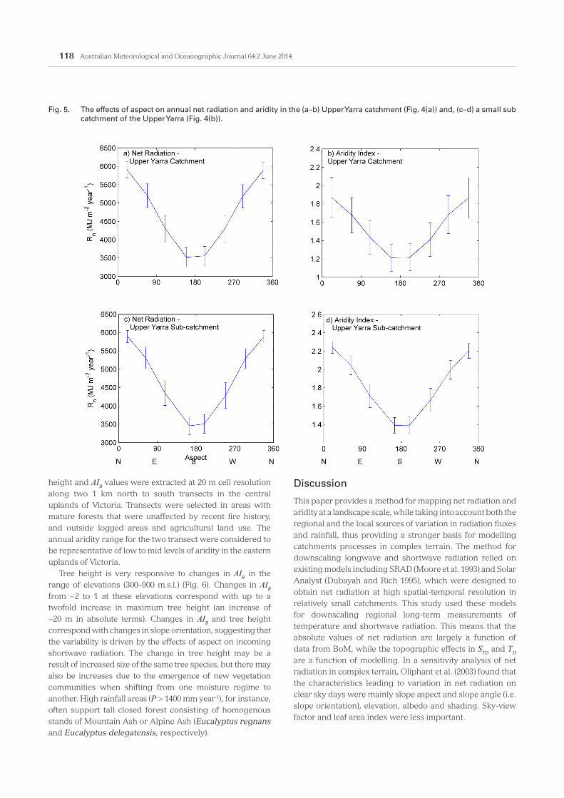
The effect of slope orientation on Rn and AIB was evaluated by grouping the typical hillslopes (25° ≤ slope ≤ 35°) into eight separate aspect categories or bins (Fig. 5). Aspect effects on net radiation, Rn, in the Upper Yarra catchment are independent of the scale at which aspect effects are quantified (Fig. 5(a) and 5(c)). On average, irrespective of the size of the study area, the average Rn on north facing slopes is ~2500 MJ m-2 year-1 higher than south facing slopes. At a large scale (Fig. 5(b)), this topographic effect on Rn translates to AIB range of 1.22–1.86 (Fig. 5(b)). At a smaller scale (Fig. 5(d)) the topographic effect is slightly larger with AIB ranging from 1.39–2.2. This means that the relative importance of aspect on variation in aridity diminishes when the spatial scale of the analysis increases (Fig. 5(b) and (d)), indicating that regional variation in rainfall (data from BoM), related to elevation, may override the effect local variation in incoming shortwave radiation due to aspect. This is consistent with the patterns of variability seen in Fig. 3 and highlights the importance in large catchments of capturing both localised topographic effects and the landscape scale effects from regional climate variability.

Variation in tree height as measure of landscape response to AIB Maximum tree height was measured in 20 m pixels using airborne lidar data and used to examine how forest biomass and limits to growth may be affected by variations in aridity. Lidar data were acquired by the Victorian Department of Environment and Primary Industries at an average density of 0.9 points per meter with a vertical and horizontal accuracy of 35 cm and 50 cm respectively. Elevation, maximum tree

Fig. 4. Annual aridity in (a) the Upper Yarra catchment (336.7 km2) in the eastern upland of Victoria, and (b) a sub-catchment (5.04 km2) of the Upper Yarra showing a north and south facing slope separated by drainage line going east to west. Note: the scale of the colour bar is specific to each figure.


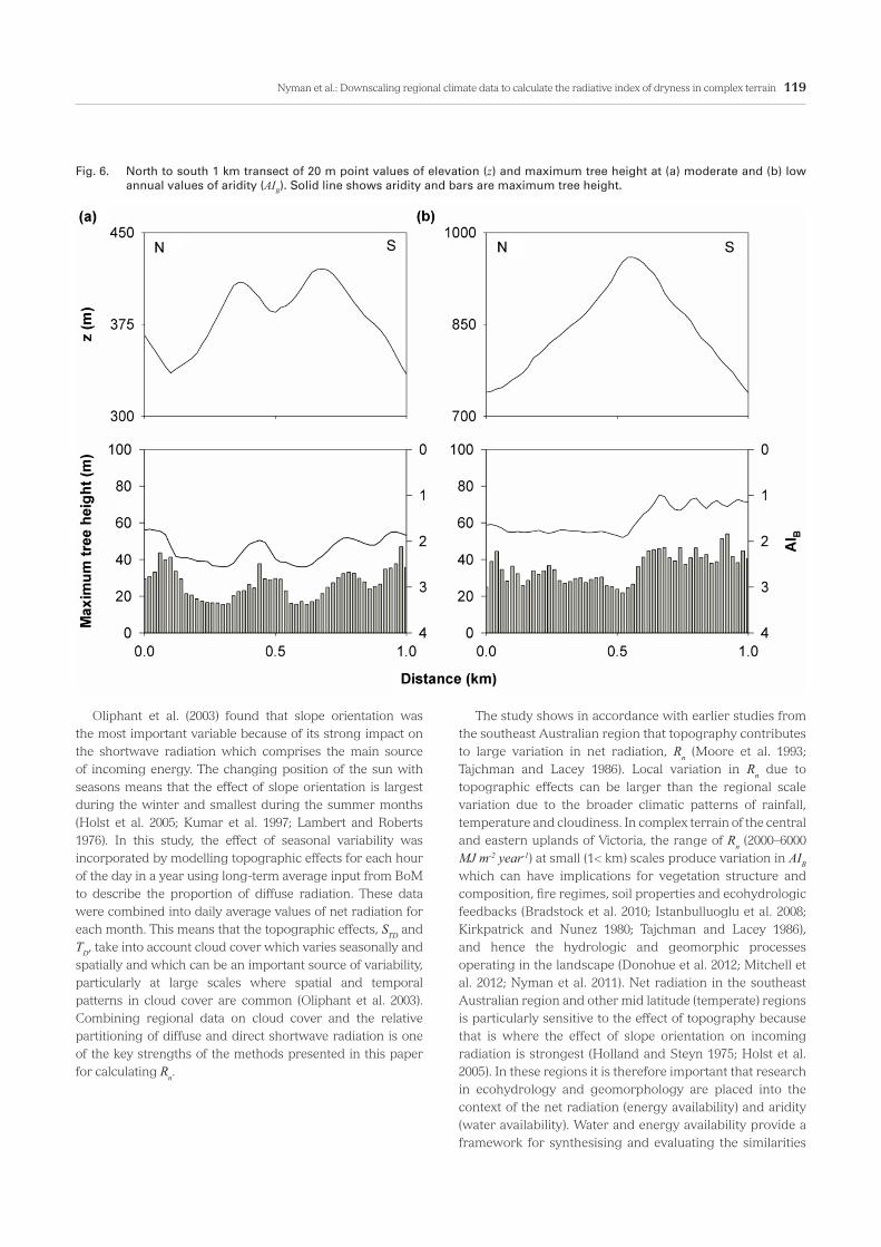
height and AIB values were extracted at 20 m cell resolution along two 1 km north to south transects in the central uplands of Victoria. Transects were selected in areas with mature forests that were unaffected by recent fire history, and outside logged areas and agricultural land use. The annual aridity range for the two transect were considered to be representative of low to mid levels of aridity in the eastern uplands of Victoria.

Tree height is very responsive to changes in AIB in the range of elevations (300–900 m.s.l.) (Fig. 6). Changes in AIB from ~2 to 1 at these elevations correspond with up to a twofold increase in maximum tree height (an increase of ~20 m in absolute terms). Changes in AIB and tree height correspond with changes in slope orientation, suggesting that the variability is driven by the effects of aspect on incoming shortwave radiation. The change in tree height may be a result of increased size of the same tree species, but there may also be increases due to the emergence of new vegetation communities when shifting from one moisture regime to another. High rainfall areas (P > 1400 mm year-1), for instance, often support tall closed forest consisting of homogenous stands of Mountain Ash or Alpine Ash (Eucalyptus regnans and Eucalyptus delegatensis, respectively).

Discussion

This paper provides a method for mapping net radiation and aridity at a landscape scale, while taking into account both the regional and the local sources of variation in radiation fluxes and rainfall, thus providing a stronger basis for modelling catchments processes in complex terrain. The method for downscaling longwave and shortwave radiation relied on existing models including SRAD (Moore et al. 1993) and Solar Analyst (Dubayah and Rich 1995), which were designed to obtain net radiation at high spatial-temporal resolution in relatively small catchments. This study used these models for downscaling regional long-term measurements of temperature and shortwave radiation. This means that the absolute values of net radiation are largely a function of data from BoM, while the topographic effects in STD and TD are a function of modelling. In a sensitivity analysis of net radiation in complex terrain, Oliphant et al. (2003) found that the characteristics leading to variation in net radiation on clear sky days were mainly slope aspect and slope angle (i.e. slope orientation), elevation, albedo and shading. Sky-view factor and leaf area index were less important.

Fig. 5. The effects of aspect on annual net radiation and aridity in the (a–b) Upper Yarra catchment (Fig. 4(a)) and, (c–d) a small sub catchment of the Upper Yarra (Fig. 4(b)).


Oliphant et al. (2003) found that slope orientation was the most important variable because of its strong impact on the shortwave radiation which comprises the main source of incoming energy. The changing position of the sun with seasons means that the effect of slope orientation is largest during the winter and smallest during the summer months (Holst et al. 2005; Kumar et al. 1997; Lambert and Roberts 1976). In this study, the effect of seasonal variability was incorporated by modelling topographic effects for each hour of the day in a year using long-term average input from BoM to describe the proportion of diffuse radiation. These data were combined into daily average values of net radiation for each month. This means that the topographic effects, STD and TD, take into account cloud cover which varies seasonally and spatially and which can be an important source of variability, particularly at large scales where spatial and temporal patterns in cloud cover are common (Oliphant et al. 2003). Combining regional data on cloud cover and the relative partitioning of diffuse and direct shortwave radiation is one of the key strengths of the methods presented in this paper for calculating Rn.

The study shows in accordance with earlier studies from the southeast Australian region that topography contributes to large variation in net radiation, Rn (Moore et al. 1993; Tajchman and Lacey 1986). Local variation in Rn due to topographic effects can be larger than the regional scale variation due to the broader climatic patterns of rainfall, temperature and cloudiness. In complex terrain of the central and eastern uplands of Victoria, the range of Rn (2000–6000 MJ m-2 year-1) at small (1< km) scales produce variation in AIB which can have implications for vegetation structure and composition, fire regimes, soil properties and ecohydrologic feedbacks (Bradstock et al. 2010; Istanbulluoglu et al. 2008; Kirkpatrick and Nunez 1980; Tajchman and Lacey 1986), and hence the hydrologic and geomorphic processes operating in the landscape (Donohue et al. 2012; Mitchell et al. 2012; Nyman et al. 2011). Net radiation in the southeast Australian region and other mid latitude (temperate) regions is particularly sensitive to the effect of topography because that is where the effect of slope orientation on incoming radiation is strongest (Holland and Steyn 1975; Holst et al. 2005). In these regions it is therefore important that research in ecohydrology and geomorphology are placed into the context of the net radiation (energy availability) and aridity (water availability). Water and energy availability provide a framework for synthesising and evaluating the similarities

Fig. 6. North to south 1 km transect of 20 m point values of elevation (z) and maximum tree height at (a) moderate and (b) low annual values of aridity (AIB). Solid line shows aridity and bars are maximum tree height.


and differences in research findings from different parts of the world. However, the methods for modelling these topographic sources of variation as part of local and regional characterisation of climate, geomorphology and eco-hydrological processes have been lacking.

Surface albedo depend on many properties including solar zenith angle, background soil type and moisture content, amount of green leaves, amount of dead leaves, leaf angle and snow properties (Hales et al. 2004; Oliphant et al. 2003). In this paper the albedo was assumed to be constant throughout the year and was modelled based on the leaf area index (Hales et al. 2004), which was assigned four different values based on forest type or land-use. For non-deciduous forests, we assumed that LAI and albedo were constant over time. This is a simplified representation of LAI and albedo and can be improved for areas where seasonality is important. On agricultural land for instance, a more realistic representation of albedo would include seasonal effects associated with grass curing, crops, and other temporal land-use effects. Furthermore, the effects of snow at high elevations were not taken into account because of the lack of long-term data on snow cover and subsequent changes in albedo. During winter the calculations will therefore overestimate the net radiation in areas above the tree line where there is consistent snow cover and where canopy effects are negligible. Improved representation of within-year variations in albedo and LAI can be incorporated into net radiation calculations by using long-term AVHRR data (e.g. Austin et al, 2013; Schaaf et al. 2002).

The exploratory correlation between tree height and AIB along transects in mountainous terrain indicate that aridity may be useful metric for predicting variability in vegetation. Future work will aim to explore these relations in more detail and develop quantitative basis for predicting ecohydrological and geomorphic processes in landscapes where water availability is variable at fine scales. This paper assumes that aridity, as a measure of water availability, is a function of rainfall and net radiation at a point and thus independent of sub-surface hydrological processes on hillslopes. This representation does not include nonlocal effects due to redistribution of water from upslope areas, nor does it include the local effects of soil depth, both of which can be important for local water availability (Daws et al. 2002; Gómez-Plaza et al. 2001). Using the AIB in the future to resolve variations in ecohydrological processes at fine spatial scales may require a model that incorporates the redistribution of excess water on hillslopes into the local water balance at each grid cell. The effects of this redistribution is likely to be most important in humid catchments because these have more available excess water than catchments situated in semi-arid environments (Gómez-Plaza et al. 2001).

Conclusion

The study describes a method for downscaling of satellite derived data on incoming radiation in order to quantify net radiation and aridity at high spatial resolution over a large area containing complex terrain. Using Victoria (southeast Australia) as a case study, the outputs show that the aridity responds to different parameters at different scales, resulting in heterogeneity and complex patterns of variability in catchment properties at scales of 10 km2 and larger. The method of combining regional climate data with models of local topographic effects will be useful for applied and theoretical studies that aim to:

1. Model landscape processes such as wildfire, erosion and fate of water and carbon in landscapes with complex terrain. These processes are sensitive to fine-scale variations in soil properties, moisture regimes, vegetation and the associated eco-hydrological feedbacks.

2. Model potential effects of climate change on water availability and vegetation dynamics. Changes caused by variation in climate can be captured most effectively when models operate at a scale and resolution which corresponds with patterns of variability in landscape properties and processes.

3. Investigate the effects of seasonality in water and energy availability as controls on ecohydrological processes. The aridity index was calculated based on the monthly values of Rn and P, and therefore provides a basis for examining the role of temporal dynamics in climate.

Acknowledgments

This study was funded by the Bushfire Cooperative Research Centre (CRC) and the Victorian Department of Environment and Primary Industries. The authors are grateful for the data provided by the Australian Bureau of Meteorology. The regional data on solar irradiance was generated by The Bureau based on satellite imagery from the Geostationary Meteorological Satellite and MTSAT series operated by Japan Meteorological Agency, and from GOES-9 operated by the National Oceanographic & Atmospheric Administration (NOAA) for the Japan Meteorological Agency. Lesley Rowland was very helpful in providing the data from The Bureau. The DEM and land-use data was provided by the Victorian Department of Environment and Primary Industries (DEPI). The authors would like to thank Dominik Jaskierniak at The University of Melbourne for assistance with coding in Python.


Symbols and units

Symbol Variable Units

AIB Aridity index (monthly or annual) dimensionless

Rn Net radiation MJ m-2 day-1or MJ m-2 year-1

λ Latent heat of evaporation MJ m-3

P Precipitation (monthly or annual) m day-1 or m year-1

TD Downscaled temperature K

Rs Daily net incoming shortwave radiation

MJ m-2day-1

Rlu Daily outgoing longwave radiation MJ m-2day-1

Rld Daily incoming longwave radiation MJ m-2day-1

αs Surface albedo dimensionless

Rg Daily global incoming radiation MJ m-2day-1

STD Topographic downscaling factor dimensionless

Ta Daily air temperature K

DHI Instantaneous solar direct horizontal irradiance

W m-2

DNI Instantaneous solar direct normal irradiance

W m-2

GNI Solar global normal irradiance W m-2

m Zenith angle of the sun radian

Rdiff Daily diffuse radiation MJ m-2 day-1

Pdiff Diffuse proportion of incoming radiation

dimensionless

Dirm Direct incoming solar radiation from Solar Analyst.

MJ m-2day-1

Diffm Diffuse incoming solar radiation from Solar Analyst

MJ m-2day-1

Rtile The mean modeled shortwave radia-tion for a tile

MJ m-2day-1

σ Stefan-Boltzman constant MJ m-2 K-4 day-1

ε_s Surface emissivity dimensionless

Tlapse Temperature lapse rate K m-1

z Elevation at each grid cell m

zb Average elevation within each 5 km x 5 km tile

m

LAI Leaf area index dimensionless

LAImax Maximum leaf area index dimensionless

εa Monthly atmospheric emissivity dimensionless

C Monthly cloud fraction dimensionless

v Sky-view factor dimensionless

ReferencesAdam J. C., Clark E. A., Lettenmaier D. P., Wood E. F. 2006. Correction of

global precipitation products for orographic effects. J. Clim., 19 (1), 15–38.

Austin J. M., Gallant J. C., Van Niel T. 2013. Mean monthly radiation sur-faces for Australia at 1 arc-second resolution. 20th International Con-gress on Modelling and Simulation, eds. J. Piantadosi, R. S. Anderssen & J. Boland, Adelaide, Australia, 1589–95.

Badano E. I. , Cavieres L. A., Molina-Montenegro M. A. , Quiroz C. L. 2005. Slope aspect influences plant association patterns in the Mediterra-nean matorral of central Chile. J. Arid Environments, 62 (1), 93–108.

Band L.E. 1993. Effect of land surface representation on forest water and carbon budgets. J. Hydro., 150 (2–4), 749–772.

Berry S. L., Farquhar G. D., Roderick M. L. 2006. Co-Evolution of Climate, Soil and Vegetation. Encyclopedia of hydrological sciences. (John Wi-ley & Sons, Ltd)

Berry S. L., Roderick M. L. 2004. Gross primary productivity and transpi-ration flux of the Australian vegetation from 1788 to 1988 AD: effects of CO2 and land use change. Global Change Biology 10 (11), 1884–98.

Boland J., Ridley B., Brown B. 2008. Models of diffuse solar radiation. Renewable Energy, 33 (4), 575–84.

Bradstock R. A., Hammill K. A., Collins L., Price O. 2010. Effects of weath-er, fuel and terrain on fire severity in topographically diverse land-scapes of south-eastern Australia. Landscape Ecology 25 (4), 607–619.

Budyko M. I. 1974. Climate and life, Academic Press: New York. Crawford T. M., Duchon C. E. 1999. An improved parameterization for

estimating effective atmospheric emissivity for use in calculating day-time downwelling longwave radiation. J. Clim., 38 (4), 474–80.

Donohue R. J., Roderick M. L., McVicar T. R. 2012. Roots, storms and soil pores: Incorporating key ecohydrological processes into Budyko’s hy-drological model. J. Hydro., 436–437 (0), 35–50.

Dubayah R., Rich P. M. 1995. Topographic solar radiation models for GIS. Int. J. Geographical Information Systems, 9 (4), 405–19.

Eamus D. 2003. How does ecosystem water balance affect net primary productivity of woody ecosystems? Functional Plant Biology, 30 (2), 187–205.

Fu P., Rich P. M. 2002. A geometric solar radiation model with applications in agriculture and forestry. Computers and Electronics in Agriculture, 37 (1–3), 25–35.

Gómez-Plaza A., Martı́nez-Mena M., Albaladejo J., Castillo V. M. 2001. Factors regulating spatial distribution of soil water content in small semiarid catchments. J. Hydro., 253 (1–4), 211–26.

Gupta S. K., Ritchey N. A., Wilber A. C., Whitlock C. H., Gibson G. G., Stackhouse P. W. 1999. A climatology of surface radiation budget de-rived from satellite data. J. Clim., 12 (8), 2691–710.

Hales K., Neelin J. D., Zeng N. 2004. Sensitivity of tropical land climate to Leaf Area Index: Role of surface conductance versus albedo. J. Clim., 17 (7), 1459–73.

Harrison L. P. 1963. Fundamental concepts and definitions relating to hu-midity. Humidity and Moisture, 3, 3–70.

Hill M. J., Senarath U., Lee A., Zeppel M., Nightingale J. M., Williams R. D. J., McVicar T. R. 2006. Assessment of the MODIS LAI product for Australian ecosystems. Remote Sensing of Environment, 101 (4), 495–518.

Holland P. G., Steyn D. G. 1975. Vegetational Responses to Latitudinal Variations in Slope Angle and Aspect. Journal of Biogeography, 2 (3), 179–83.

Holst T., Rost J., Mayer H. 2005. Net radiation balance for two forested slopes on opposite sides of a valley. International Journal of Biometeo-rology, 49 (5), 275–84.

Hutchinson M. F. 1998. Interpolation of rainfall data with thin plate smoothing splines. Part I: Two dimensional smoothing of data with short range correlation. Journal of Geographic Information and Deci-sion Analysis, 2 (2), 139–51.

Istanbulluoglu E., Yetemen O., Vivoni E. R., Gutiérrez-Jurado H. A., and Bras R. L. 2008. Eco-geomorphic implications of hillslope aspect: In-ferences from analysis of landscape morphology in central New Mex-ico. Geophys. Res. Lett., 35, L14403.

Australian Meteorological and Oceanographic Journal 64 (2014) 109–122

122

Kirkpatrick J., Nunez M. 1980. Vegetation-radiation relationships in mountainous terrain: eucalypt-dominated vegetation in the Risdon Hills, Tasmania. Journal of Biogeography, 197–208.

Kumar L., Skidmore A. K., Knowles E. 1997. Modelling topographic varia-tion in solar radiation in a GIS environment. International Journal of Geographical Information Science, 11 (5), 475–97.

Lambert M., Roberts E. 1976. Aspect differences in an unimproved hill country pasture: I. Climatic differences. New Zealand journal of Agri-cultural, 19 (4), 459–67.

Lane P. N. J., Feikema P. M., Sherwin C. B., Peel M. C., Freebairn A. C. 2010. Modelling the long-term water yield impact of wildfire and oth-er forest disturbance in Eucalypt forests. Environmental Modelling & Software, 25 (4), 467–78.

Mitchell P. J., Lane P. N. J., Benyon R. G. 2012. Capturing within catch-ment variation in evapotranspiration from montane forests using LiDAR canopy profiles with measured and modelled fluxes of water. Ecohydrology, 5 (6), 708–20.

Moore I. D., Norton T. W., Williams J. E. 1993. Modelling environmental heterogeneity in forested landscapes. J. Hydro., 150 (2–4), 717–47.

Nemani R. R., Keeling C. D., Hashimoto H., Jolly W. M., Piper S. C., Tucker C. J., Myneni R. B., Running S. W. 2003. Climate-driven increases in global terrestrial net primary production from 1982 to 1999. Science, 300 (5625), 1560–63.

Niklas K.J. 2007. Maximum plant height and the biophysical factors that limit it. Tree Physiology, 27 (3), 433–40.

Nilsson M. 1996. Estimation of tree heights and stand volume using an airborne lidar system. Remote Sensing of Environment, 56 (1), 1–7.

Nunez M. 1980. The Calculation of solar and net radiation in mountainous terrain. Journal of Biogeography, 7 (2), 173–86.

Nyman P., Sheridan G. J., Smith H. G., Lane P. N. J. 2011. Evidence of de-bris flow occurrence after wildfire in upland catchments of south-east Australia. Geomorphology, 125 (3), 383–401.

Ohring G., Clapp P. 1980. The effect of changes in cloud amount on the net Radiation at the top of the Atmosphere. J. Atmos. Sci., 37 (2), 447–54.

Ohta S., Uchijima Z., Oshima Y. 1993. Probable effects of CO2-induced cli-matic changes on net primary productivity of terrestrial vegetation in East Asia. Ecological Research, 8 (2), 199–213.

Oliphant A., Spronken-Smith R., Sturman A., Owens I. 2003. Spatial vari-ability of surface radiation fluxes in mountainous terrain. J. Appl. Me-teorol., 42 (1), 113–28.

Pierce L., Walker J., Dowling T., McVicar T., Hatton T., Running S., Cough-lan J. 1993. Ecohydrological changes in the Murray-Darling Basin. III. A simulation of regional hydrological changes. Journal of Applied Ecology, 283–94.

Rasmusson E. M., Arkin P. A. 1993. A global view of large-scale pre-cipitation variability. J. Clim., 6 (8), 1495–1522.

Ridley B., Boland J., Lauret P. 2010. Modelling of diffuse solar fraction with multiple predictors. Renewable Energy, 35 (2), 478–83.

Running S. W., Nemani R. R., Hungerford R. D. 1987. Extrapolation of synoptic meteorological data in mountainous terrain and its use for simulating forest evapotranspiration and photosynthesis. Canadian Journal of Forest Research, 17 (6), 472–83.

Running S. W., Thornton P. E., Nemani R., Glassy J. M. 2000. Global ter-restrial gross and net primary productivity from the Earth Observing System. Methods in Ecosystem Science, 44–57.

Schaaf C. B., Gao F., Strahler A. H., Lucht W., Li X., Tsang T. et al. 2002. First operational BRDF, albedo nadir reflectance products from MO-DIS. Remote Sensing of Environment, 83, 135–48.

Swinbank W. C. 1963. Longwave radiation from clear skies. Q. J. R. Me-teorol. Soc., 89 (381), 339–48.

Tajchman S. J., Lacey C. J. 1986. Bioclimatic factors in forest site potential. Forest Ecology and Management, 14 (3), 211–18.

Victorian Department of Environment and Primary Industries. 2011. Ecological vegetation classes by bioregion. www.dse.vic.gov.au/conservation-and-environment/native-vegetation-groups-for-victoria/?a=89375

Weymouth G. T., Le Marshall J. F . 2001. Estimation of daily surface so-lar exposure using GMS-5 stretched-VISSR observations : the system and basic results. Aust. Meteorol. Mag., 50 (4), 263–78.

Wilson J. P., Gallant J. C. 2000. Secondary topographic attributes. Terrain analysis : principles and applications. Ed. JCG John P. Wilson. (New York : J. Wiley)

Xu T., Hutchinson M. 2011. ANUCLIM Version 6.1 User Guide. The Aus-tralian National University, Fenner School of Environment and Soci-ety, Canberra.

downscaling regional climate data to calculate the ... · pdf filenyman et al.: downscaling...

Documents