downscaling precipitation to river basin in india for ipcc sres scenarios using support vector...

INTERNATIONAL JOURNAL OF CLIMATOLOGYInt. J. Climatol. 28: 401–420 (2008)Published online 18 June 2007 in Wiley InterScience(www.interscience.wiley.com) DOI: 10.1002/joc.1529

Downscaling precipitation to river basin in India for IPCCSRES scenarios using support vector machine

Aavudai Anandhi,a V. V. Srinivas,a Ravi S. Nanjundiahb and D. Nagesh Kumara*a Department of Civil Engineering, Indian Institute of Science, Bangalore, India

b Center for Atmospheric and Oceanic Sciences, Indian Institute of Science, Bangalore, India

ABSTRACT: This paper presents a methodology to downscale monthly precipitation to river basin scale in Indian contextfor special report of emission scenarios (SRES) using Support Vector Machine (SVM). In the methodology presented,probable predictor variables are extracted from (1) the National Center for Environmental Prediction (NCEP) reanalysisdata set for the period 1971–2000 and (2) the simulations from the third generation Canadian general circulation model(CGCM3) for SRES emission scenarios A1B, A2, B1 and COMMIT for the period 1971–2100. These variables includeboth the thermodynamic and dynamic parameters and those which have a physically meaningful relationship with theprecipitation. The NCEP variables which are realistically simulated by CGCM3 are chosen as potential predictors forseasonal stratification. The seasonal stratification involves identification of (1) the past wet and dry seasons throughclassification of the NCEP data on potential predictors into two clusters by the use of K-means clustering algorithmand (2) the future wet and dry seasons through classification of the CGCM3 data on potential predictors into two clustersby the use of nearest neighbour rule. Subsequently, a separate downscaling model is developed for each season to capturethe relationship between the predictor variables and the predictand. For downscaling precipitation, the predictand is chosenas monthly Thiessen weighted precipitation for the river basin, whereas potential predictors are chosen as the NCEPvariables which are correlated to the precipitation and are also realistically simulated by CGCM3. Implementation of themethodology presented is demonstrated by application to Malaprabha reservoir catchment in India which is considered tobe a climatically sensitive region. The CGCM3 simulations are run through the calibrated and validated SVM downscalingmodel to obtain future projections of predictand for each of the four emission scenarios considered. The results showthat the precipitation is projected to increase in future for almost all the scenarios considered. The projected increase inprecipitation is high for A2 scenario, whereas it is least for COMMIT scenario. Copyright 2007 Royal MeteorologicalSociety

KEY WORDS climate change; downscaling; hydroclimatology; precipitation; support vector machine (SVM); IPCC SRESscenarios; clustering

Received 30 November 2006; Revised 19 February 2007; Accepted 24 February 2007

1. Introduction

It is necessary to access the past and assess the futureprecipitation and its variability at different timescalesto study the impact of climate change on the follow-ing: (1) hydrology (Cohen et al., 2000; Gosain et al.,2006; Menzel et al., 2006; Yaning et al., 2006); (2)water resources management (Krasovskaia, 1995; Risbyand Entekhabi, 1996; Kabat and van Schaik, 2003); (3)agriculture (Darwin et al., 1995; Adams et al., 1998;Selvaraju, 2003); (4) forestry (Kirilenko and Solomon,1998); (5), floods (Mirza et al., 1998; Reynard et al.,1998; Miller et al., 2004); (6) droughts (Vicente–Serranoand Lopez–Moreno, 2006); (7) soil erosion (Valentin,1996; Gregory et al., 1999); (8) land use change (IPCC,2001); (9) groundwater (Sandstrom, 1995; Allen andScibek, 2006); (10) environment (Jones and Jongen,1996; Coughenour and Chen, 1997); (11) tourism (More,

* Correspondence to: D. Nagesh Kumar, Department of Civil Engi-neering, Indian Institute of Science, Bangalore, India.E-mail: [email protected]

1988; Richardson, 2003; Wamukonya, 2003); (12) humanand animal population (Brotton and Wall, 1997; Fergu-son, 1999) and their health (Tyler, 1994; Hamilton, 1995;Pounds et al., 1999).

A proper assessment of probable future precipitationand its variability is to be made for various climate sce-narios. These scenarios refer to plausible future climateswhich have been constructed for explicit use in investigat-ing the potential consequences of anthropogenic climatechange and natural climate variability. Since climate sce-narios envisage assessment of future developments incomplex systems, they are often inherently unpredictable,insufficiently assessed, and have high scientific uncertain-ties (Carter et al., 2001). So, it is preferable to considera range of scenarios in climate impact studies as suchan approach better reflects the uncertainties of the possi-ble future climate change (Houghton et al., 2001). Thescenarios considered in this study are relevant to thefourth assessment report of the Intergovernmental Panelon Climate Change (IPCC), which is to be released in2007.

Copyright 2007 Royal Meteorological Society

402 A. ANANDHI ET AL.

General circulation models (GCMs) are among themost advanced tools, which use transient climate simu-lations to simulate climatic conditions on earth hundredsof years into the future. In a transient simulation, anthro-pogenic forcings, which are mostly decided on the basisof IPCC climate scenarios, are changed gradually in arealistic fashion. The GCMs are usually run at coarse gridresolution and as a result they are inherently unable torepresent sub-grid scale features like orography and landuse, and dynamics of mesoscale processes. Consequently,outputs from these models cannot be used directly forclimate impact assessment on a local scale. Hence inthe past decade, several downscaling methodologies havebeen developed to transfer the GCM simulated informa-tion to local scale. In general, local scale is defined onthe basis of geographical, political or physiographic con-siderations.

This study is motivated by a desire to develop effectivedownscaling model using a novel machine learningtechnique called Support Vector Machine (SVM), toassess implications of climate change on precipitation inMalaprabha river basin of India, which is considered to bea climatically sensitive region. Herein a river basin refersto the portion of land drained by many streams and creeksthat flow downhill to form tributaries to the main river.It is necessary to assess the impact of climate changeon river basin scale, as such a scale integrates some ofthe important systems like ecological and socioeconomicsystems and is closely linked with the availability ofdrinking water which is one of the most vulnerableresources of the world.

The remainder of this paper is structured as follows:Section 2 presents an overview of downscaling modelsand the underlying principle of SVM which is used in thisstudy to translate information from GCMs to local scale.Section 3 provides a description of the study region andmotivation for its selection. Section 4 provides detailsof data used in the study. Section 5 describes probablepredictor variables considered in the study and explainsthe reasons behind their selection. Section 6 presentsthe procedure proposed for seasonal stratification. Sec-tion 7 describes the methodology proposed for develop-ment of SVM model for downscaling precipitation to ariver basin. Section 8 presents the results and discus-sion. Finally, Section 9 provides a summary of the workpresented in this paper and conclusions drawn from thestudy.

2. Methods of downscaling

This section briefly outlines the various downscalingmethods available in literature. The two downscalingapproaches that are being pursued currently are dynamicdownscaling and statistical downscaling. In the dynamicdownscaling approach, a Regional Climate Model (RCM)is nested into GCM. The RCM is essentially a numericalmodel in which GCMs are used to fix boundary condi-tions. The major drawback of RCM, which restricts its

use in climate impact studies, is its complicated designand high computational cost. Moreover, RCM is inflex-ible in the sense that expanding the region or movingto a slightly different region requires redoing the entireexperiment (Crane and Hewitson, 1998). Dynamic down-scaling can be further subdivided into one-way nestingand two-way nesting (Wang et al., 2004).

The Statistical downscaling involves developing quan-titative relationships between large-scale atmosphericvariables (predictors) and local surface variables (predic-tands). There are three types of statistical downscalingnamely, weather classification methods, weather genera-tors and transfer functions. The most common statisticaldownscaling approaches are based on transfer functions,which model direct relationships between predictors andpredictands (Schoof et al., 2007). The transfer functionsare conceptually simple means of representing linearor nonlinear relationships between predictors and pre-dictands. Examples of transfer function based statisticaldownscaling methods include those which use linear andnonlinear regression, artificial neural networks, canonicalcorrelation and principal component analysis (PCA).

In recent times, SVM approach is recognized forits ability to capture nonlinear regression relationshipsbetween variables (Vapnik, 1995; Vapnik, 1998; Haykin,2003). The SVMs implement the structural risk mini-mization principle which attempts to minimize an upperbound on the generalization error, by striking a rightbalance between the training error and the capacity ofmachine (i.e. the ability of machine to learn any trainingset without error). Global optimum solution is guaran-teed with SVM (Haykin, 2003). Further, for the SVMsthe learning algorithm automatically decides the modelarchitecture (number of hidden units). The flexibility ofthe SVM is provided by the use of kernel functions thatimplicitly map the data to a higher, possibly infinite,dimensional space. A linear solution in the higher dimen-sional feature space corresponds to a nonlinear solutionin the original lower dimensional input space. This makesSVM a feasible choice for downscaling problems whichare nonlinear in nature. Recently, Tripathi et al. (2006)proposed the SVM approach for downscaling precipita-tion to meteorological subdivisions in India.

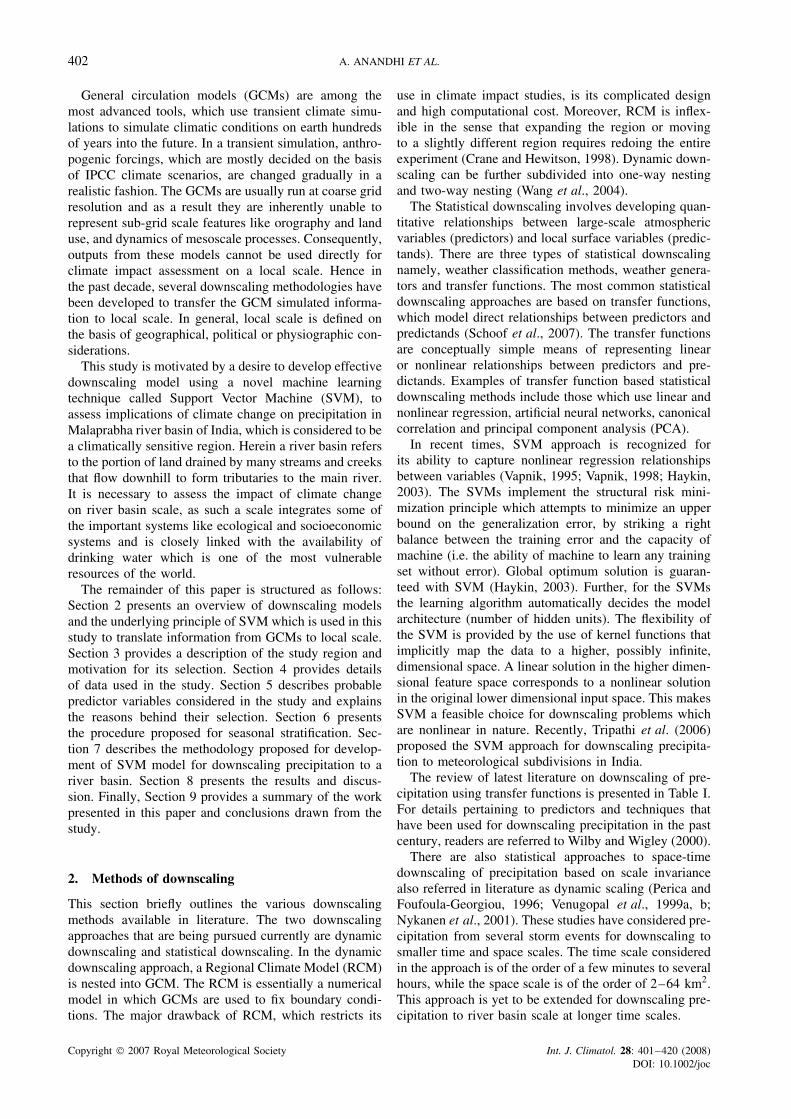
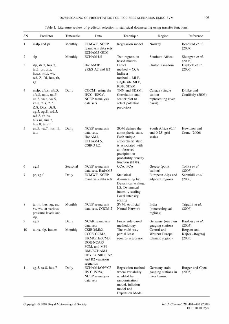
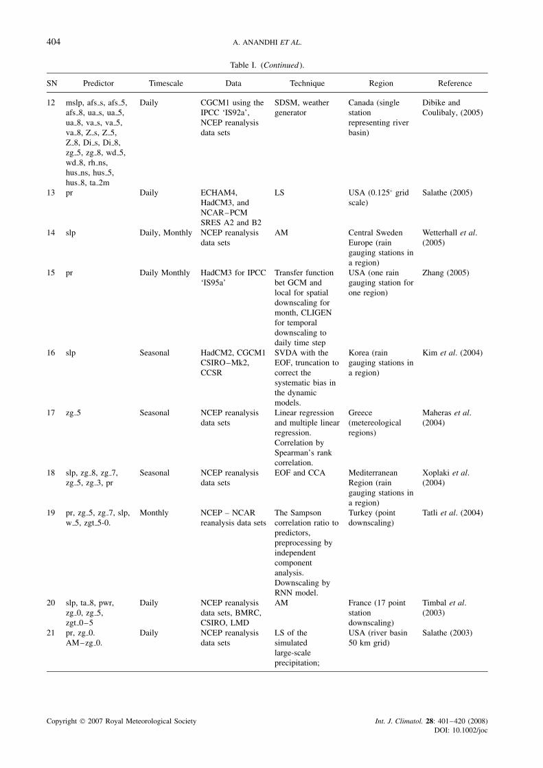
The review of latest literature on downscaling of pre-cipitation using transfer functions is presented in Table I.For details pertaining to predictors and techniques thathave been used for downscaling precipitation in the pastcentury, readers are referred to Wilby and Wigley (2000).

There are also statistical approaches to space-timedownscaling of precipitation based on scale invariancealso referred in literature as dynamic scaling (Perica andFoufoula-Georgiou, 1996; Venugopal et al., 1999a, b;Nykanen et al., 2001). These studies have considered pre-cipitation from several storm events for downscaling tosmaller time and space scales. The time scale consideredin the approach is of the order of a few minutes to severalhours, while the space scale is of the order of 2–64 km2.This approach is yet to be extended for downscaling pre-cipitation to river basin scale at longer time scales.

Copyright 2007 Royal Meteorological Society Int. J. Climatol. 28: 401–420 (2008)DOI: 10.1002/joc

DOWNSCALING OF PRECIPITATION FOR IPCC SRES SCENARIOS USING SVM 403

Table I. Literature review of predictor selection in statistical downscaling using transfer functions.

SN Predictor Timescale Data Technique Region Reference

1 mslp and pr Monthly ECMWF, NCEPreanalysis data sets

Regression model Norway Benestad et al.(2007)

ECHAM5 GCM2 slp Monthly ECHAM4.5 Two regression

based modelsSouthern Africa Shongwe et al.

(2006)3 slp, rh 7, hus 7,

ta 7, ps, ta s,hus s, rh s, ws,wd, Z, Di, hus, rh,zg

HadAM3PSRES A2 and B2

Directmethod – CCAIndirectmethod – MLP,single site MLP,RBF, SDSM.

United Kingdom Haylock et al.(2006)

4 mslp, afs s, afs 5,afs 8, ua s, ua 5,ua 8, va s, va 5,va 8, Z s, Z 5,Z 8, Di s, Di 8,zg 5, zg 8, wd 5,wd 8, rh ns,hus ns, hus 5,hus 8, ta 2m

Daily CGCM1 using theIPCC ‘IS92a’,NCEP reanalysisdata sets

TNN and SDSM;Correlation andscatter plot toselect potentialpredictors

Canada (singlestationrepresenting riverbasin)

Dibike andCoulibaly (2006)

5 ua 7, va 7, hus, rh,ta s

Daily NCEP reanalysisdata sets,HadAM3,ECHAM4.5,CSIRO k2.

SOM defines theatmospheric state.Each uniqueatmospheric stateis associated withan observedprecipitationprobability densityfunction (PDF).

South Africa (0.1°

and 0.25° gridscale)

Hewitson andCrane (2006)

6 zg 5 Seasonal NCEP reanalysisdata sets, HadAM3

CCA, PCA Greece (pointstation)

Tolika et al.(2006).

7 pr, zg 0 Daily ECMWF, NCEPreanalysis data sets

Statisticaldownscaling byDynamical scaling,LS, Dynamicalintensity scaling,Local intensityscaling

European Alps andadjacent regions

Schmidli et al.(2006)

8 ta, rh, hus, zg, ua,va, wa, at variouspressure levels andslp.

Monthly NCEP reanalysisdata sets, CGCM 2

SVM, ArtificialNeural Network

India(metereologicalregions)

Tripathi et al.(2006)

9 zg 7 Daily NCAR reanalysisdata sets

Fuzzy rule-basedmethodology

Germany (one raingauging station)

Bardossy et al.(2005)

10 ta ns, slp, hus ns Monthly CSIRO/Mk2,CCC/CGCM2,UKMO/HadCM3,DOE-NCAR/PCM, and MPI-DMI/ECHAM4-OPYC3. SRES A2and B2 emissionscenarios

The multi-waypartial leastsquares regression

Central andWestern Europe(climate region)

Bergant andKajfez–Bogataj(2005)

11 zg 5, ta 8, hus 7 Daily ECHAM4/OPYC3IPCC IS95a,NCEP reanalysisdata sets

Regression methodwhere variabilityis added byrandomizationmodel, inflationmodel andExpansion Model

Germany (raingauging stations inriver basins)

Burger and Chen(2005)



Table I. (Continued ).


12 mslp, afs s, afs 5,afs 8, ua s, ua 5,ua 8, va s, va 5,va 8, Z s, Z 5,Z 8, Di s, Di 8,zg 5, zg 8, wd 5,wd 8, rh ns,hus ns, hus 5,hus 8, ta 2m

Daily CGCM1 using theIPCC ‘IS92a’,NCEP reanalysisdata sets

SDSM, weathergenerator

Canada (singlestationrepresenting riverbasin)

Dibike andCoulibaly, (2005)

13 pr Daily ECHAM4,HadCM3, andNCAR–PCMSRES A2 and B2

LS USA (0.125° gridscale)

Salathe (2005)

14 slp Daily, Monthly NCEP reanalysisdata sets

AM Central SwedenEurope (raingauging stations ina region)

Wetterhall et al.(2005)

15 pr Daily Monthly HadCM3 for IPCC‘IS95a’

Transfer functionbet GCM andlocal for spatialdownscaling formonth, CLIGENfor temporaldownscaling todaily time step

USA (one raingauging station forone region)

Zhang (2005)

16 slp Seasonal HadCM2, CGCM1CSIRO–Mk2,CCSR

SVDA with theEOF, truncation tocorrect thesystematic bias inthe dynamicmodels.

Korea (raingauging stations ina region)

Kim et al. (2004)

17 zg 5 Seasonal NCEP reanalysisdata sets

Linear regressionand multiple linearregression.Correlation bySpearman’s rankcorrelation.

Greece(metereologicalregions)

Maheras et al.(2004)

18 slp, zg 8, zg 7,zg 5, zg 3, pr

Seasonal NCEP reanalysisdata sets

EOF and CCA MediterraneanRegion (raingauging stations ina region)

Xoplaki et al.(2004)

19 pr, zg 5, zg 7, slp,w 5, zgt 5-0.

Monthly NCEP – NCARreanalysis data sets

The Sampsoncorrelation ratio topredictors,preprocessing byindependentcomponentanalysis.Downscaling byRNN model.

Turkey (pointdownscaling)

Tatli et al. (2004)

20 slp, ta 8, pwr,zg 0, zg 5,zgt 0–5

Daily NCEP reanalysisdata sets, BMRC,CSIRO, LMD

AM France (17 pointstationdownscaling)

Timbal et al.(2003)

21 pr, zg 0.AM–zg 0.

Daily NCEP reanalysisdata sets

LS of thesimulatedlarge-scaleprecipitation;

USA (river basin50 km grid)

Salathe (2003)



Table I. (Continued ).


22 Lag-1 predictand,Wet, T mean,hus ns, RH ns,mslp, ua, va, F, Z,zg 5,

NCEP reanalysisdata sets, CGCM1-greenhouse-gas-plus-sulphate-aerosolsexperiment

SDSM Canada (regionToronto)

Wilby et al. (2002)

23 zg 7, zg 5, pr Daily Observed stations Classificationpattern based onfuzzy rule.Multivariatestochasticdownscaling foreach pattern.

Germany (8 pointstations), Greece(21 point stations)

Stehlik andBardossy (2002)

24 Indices such asCAPE, CI, BRN,WS, SWTI

Minutes, hours 47 selected radarscans, MM5

Spatial-temporaldownscaling.Relation betweenindices and scaleindependentparameter.

Central USA(single storms of2 days, 4–64 km)

Nykanen et al.(2001)

Note: Abbreviations are explained in Appendix.

In the current study, the objective is to effectivelydownscale precipitation from tens of thousands of km2

(i.e. spatial domain of predictor variables) to a riverbasin with an area of 2500 km2 at monthly timescale.To the knowledge of the authors, no studies have beencarried out in India on downscaling precipitation to ariver basin scale nor are we aware of any prior workaimed at downscaling third generation Canadian generalcirculation model (CGCM3) simulations to river basinscale for various IPCC scenarios using SVM approach.

2.1. Least square support vector machine

The Least Square Support Vector Machine (LS-SVM)has been used in this study to downscale precipitation.The LS-SVM provides a computational advantage overstandard SVM (Suykens, 2001). This section presents anunderlying principle of the LS-SVM

Consider a finite training sample of N patterns{(xi , yi), i = 1, . . . , N}, where xi denoting the ‘i-th’ pat-tern in n-dimensional space (i.e. xi = [x1i , . . . , xni] ∈�n) constitutes input to LS-SVM and yi ∈ � is the cor-responding value of the desired model output. Further,let the learning machine be defined by a set of possiblemappings x �→ f (x, w), where f (·) is a deterministicfunction which, for a given input pattern x and adjustableparameters w (w ∈ �n), always gives the same output.Training phase of the learning machine involves adjust-ing the parameters w. The parameters are estimated byminimizing the cost function �L(w, e). The LS-SVMoptimization problem for function estimation is formu-lated by minimizing the cost function.

�L(w, e) = 1

2wT w + 1

2C

N∑i=1

e2i

subject to the equality constraint

yi − yi = ei i = 1, . . . , N (1)

where C is a positive real constant and y is theactual model output. The first term of the cost functionrepresents weight decay or model complexity-penaltyfunction. It is used to regularize weight sizes andto penalize large weights. This helps in improvinggeneralization performance (Hush and Horne, 1993).The second term of the cost function represents penaltyfunction.

The solution of the optimization problem is obtainedby considering the Lagrangian as

L(w, b, e, α) = 1

2wTw + 1

2C

N∑i=1

e2i −

N∑i=1

αi{yi + ei − yi}

(2)

where αi are Lagrange multipliers and b is the bias term.The conditions for optimality are given by

∂L∂w = w − ∑N

i=1 αiφ(xi ) = 0∂L∂b

= ∑Ni=1 αi = 0

∂L∂ei

= αi − Cei = 0 i = 1, . . . , N

∂L∂αi

= yi + ei − yi = 0 i = 1, . . . , N

(3)

The above conditions of optimality can be expressedas the solution to the following set of linear equations



after elimination of w and ei .[0 �1T

�1 � + C−1I

] [b

α

]=

[0

y

]

where y =

y1

y2...

yN

; �1 =

11...

1

N×1

;

α =

α1

α2...

αN

; I =

1 0 . . . 00 1 . . . 0...

......

...

0 0 . . . 1

N×N

(4)

In Equation (4), � is obtained from the application ofMercer’s theorem.

�i,j = K(xi , xj ) = φ(xj )T φ(xj ) ∀i, j (5)

where φ(·) represents nonlinear transformation functiondefined to convert a non linear problem in the originallower dimensional input space to linear problem in ahigher dimensional feature space.

The resulting LS-SVM model for function estimationis:

f (x) =∑

αi∗ K(xi , x) + b∗ (6)

where α∗i and b∗ are the solutions to Equation (4) and

K(xi , x) is the inner product kernel function definedin accordance with Mercer’s theorem (Mercer, 1909;Courant and Hilbert, 1970) and b∗ is the bias. Thereare several possibilities for the choice of kernel function,including linear, polynomial, sigmoid, splines and radialbasis function (RBF). The linear kernel is a special caseof RBF (Keerthi and Lin, 2003). Further, the sigmoidkernel behaves like RBF for certain parameters (Linand Lin, 2003). In this study RBF is used to map theinput data into higher dimensional feature space, whichis given by:

K(xi , xj ) = exp

(−‖xi − xj‖2

σ

)(7)

where, σ is the width of RBF kernel, which can beadjusted to control the expressivity of RBF. The RBFkernels have localized and finite responses across theentire range of predictors.

The advantage with RBF kernel is that it nonlinearlymaps the training data into a possibly infinite-dimensionalspace and thus it can effectively handle the situationswhen the relationship between predictors and predictandis nonlinear. Moreover, the RBF is computationally sim-pler than polynomial kernel, which has more parameters.It is worth mentioning that developing LS-SVM withRBF kernel involves selection of RBF kernel width σ

and parameter C.In the present study the LS-SVM model, which has

been proven to be effective for downscaling precipitation

to Indian meteorological subdivisions in an earlier work(Tripathi et al., 2006), is developed for implementationat river basin scale. The scale of meteorological subdi-vision used by Tripathi et al. (2006) is much larger thanthat of the river basin used in the present study. The effec-tiveness of the developed model is demonstrated throughapplication to downscale precipitation in catchment ofMalaprabha reservoir from simulations of the third gen-eration CGCM3 for latest IPCC scenarios namely, A1B,A2, B1 and COMMIT. In the earlier work (Tripathi et al.,2006), simulations of second generation Canadian Gen-eral Circulation Model for IS92a scenario are used fordownscaling precipitation. The IS92a scenario, whichis also known as Business-as-usual scenario, considersemissions to grow at the present rate. The scenarios A1B,A2, B1 and COMMIT which are considered in the presentstudy provide a more meaningful basis for impact esti-mates because they are based on different viewpoints onpossible future development pathways and include themajor driving forces behind human development such aseconomic, demographic, social and technological changeother than anthropogenic emissions. Each of the scenariosis explained briefly in Table II. Further, issues associatedwith seasonal stratification and downscaling using SVMmodel are also discussed in the present study.

3. Study region

The study region is the catchment of Malaprabha river,upstream of Malaprabha reservoir in Karnataka stateof India. It has an area of 2564 km2 situated between15°30′N and 15°56′N latitudes and 74°12′E and 75°15′Elongitudes. It receives an average annual precipitationof 1051 mm. It has a tropical monsoon climate wheremost of the precipitation is confined to a few months ofthe monsoon season (Figure 1). The south–west (sum-mer) monsoon has warm winds blowing from the IndianOcean causing copious amount of precipitation duringJune–September months. The Malaprabha basin is one ofthe major lifelines for the arid regions of north Karnataka

0

50

100

150

200

250

300

350

Jan Feb Mar Apl May Jun Jul Aug Sep Oct Nov Dec

Month

Pre

cipi

tatio

n (m

m)

Figure 1. Thiessen Weighted Precipitation (TWP) for the study region.This figure is available in colour online at www.interscience.wiley.

com/ijoc



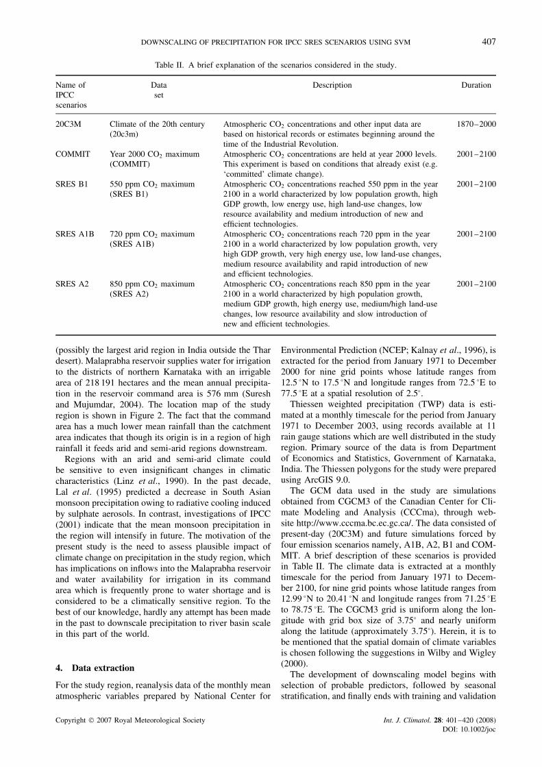
Table II. A brief explanation of the scenarios considered in the study.

Name ofIPCCscenarios

Dataset

Description Duration

20C3M Climate of the 20th century(20c3m)

Atmospheric CO2 concentrations and other input data arebased on historical records or estimates beginning around thetime of the Industrial Revolution.

1870–2000

COMMIT Year 2000 CO2 maximum(COMMIT)

Atmospheric CO2 concentrations are held at year 2000 levels.This experiment is based on conditions that already exist (e.g.‘committed’ climate change).

2001–2100

SRES B1 550 ppm CO2 maximum(SRES B1)

Atmospheric CO2 concentrations reached 550 ppm in the year2100 in a world characterized by low population growth, highGDP growth, low energy use, high land-use changes, lowresource availability and medium introduction of new andefficient technologies.

2001–2100

SRES A1B 720 ppm CO2 maximum(SRES A1B)

Atmospheric CO2 concentrations reach 720 ppm in the year2100 in a world characterized by low population growth, veryhigh GDP growth, very high energy use, low land-use changes,medium resource availability and rapid introduction of newand efficient technologies.

2001–2100

SRES A2 850 ppm CO2 maximum(SRES A2)

Atmospheric CO2 concentrations reach 850 ppm in the year2100 in a world characterized by high population growth,medium GDP growth, high energy use, medium/high land-usechanges, low resource availability and slow introduction ofnew and efficient technologies.

2001–2100

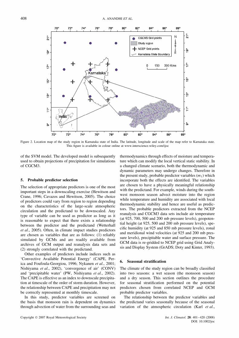
(possibly the largest arid region in India outside the Thardesert). Malaprabha reservoir supplies water for irrigationto the districts of northern Karnataka with an irrigablearea of 218 191 hectares and the mean annual precipita-tion in the reservoir command area is 576 mm (Sureshand Mujumdar, 2004). The location map of the studyregion is shown in Figure 2. The fact that the commandarea has a much lower mean rainfall than the catchmentarea indicates that though its origin is in a region of highrainfall it feeds arid and semi-arid regions downstream.

Regions with an arid and semi-arid climate couldbe sensitive to even insignificant changes in climaticcharacteristics (Linz et al., 1990). In the past decade,Lal et al. (1995) predicted a decrease in South Asianmonsoon precipitation owing to radiative cooling inducedby sulphate aerosols. In contrast, investigations of IPCC(2001) indicate that the mean monsoon precipitation inthe region will intensify in future. The motivation of thepresent study is the need to assess plausible impact ofclimate change on precipitation in the study region, whichhas implications on inflows into the Malaprabha reservoirand water availability for irrigation in its commandarea which is frequently prone to water shortage and isconsidered to be a climatically sensitive region. To thebest of our knowledge, hardly any attempt has been madein the past to downscale precipitation to river basin scalein this part of the world.

4. Data extraction

For the study region, reanalysis data of the monthly meanatmospheric variables prepared by National Center for

Environmental Prediction (NCEP; Kalnay et al., 1996), isextracted for the period from January 1971 to December2000 for nine grid points whose latitude ranges from12.5 °N to 17.5 °N and longitude ranges from 72.5 °E to77.5 °E at a spatial resolution of 2.5°.

Thiessen weighted precipitation (TWP) data is esti-mated at a monthly timescale for the period from January1971 to December 2003, using records available at 11rain gauge stations which are well distributed in the studyregion. Primary source of the data is from Departmentof Economics and Statistics, Government of Karnataka,India. The Thiessen polygons for the study were preparedusing ArcGIS 9.0.

The GCM data used in the study are simulationsobtained from CGCM3 of the Canadian Center for Cli-mate Modeling and Analysis (CCCma), through web-site http://www.cccma.bc.ec.gc.ca/. The data consisted ofpresent-day (20C3M) and future simulations forced byfour emission scenarios namely, A1B, A2, B1 and COM-MIT. A brief description of these scenarios is providedin Table II. The climate data is extracted at a monthlytimescale for the period from January 1971 to Decem-ber 2100, for nine grid points whose latitude ranges from12.99 °N to 20.41 °N and longitude ranges from 71.25 °Eto 78.75 °E. The CGCM3 grid is uniform along the lon-gitude with grid box size of 3.75° and nearly uniformalong the latitude (approximately 3.75°). Herein, it is tobe mentioned that the spatial domain of climate variablesis chosen following the suggestions in Wilby and Wigley(2000).

The development of downscaling model begins withselection of probable predictors, followed by seasonalstratification, and finally ends with training and validation



Figure 2. Location map of the study region in Karnataka state of India. The latitude, longitude and scale of the map refer to Karnataka state.This figure is available in colour online at www.interscience.wiley.com/ijoc

of the SVM model. The developed model is subsequentlyused to obtain projections of precipitation for simulationsof CGCM3.

5. Probable predictor selection

The selection of appropriate predictors is one of the mostimportant steps in a downscaling exercise (Hewitson andCrane, 1996; Cavazos and Hewitson, 2005). The choiceof predictors could vary from region to region dependingon the characteristics of the large-scale atmosphericcirculation and the predictand to be downscaled. Anytype of variable can be used as predictor as long as itis reasonable to expect that there exists a relationshipbetween the predictor and the predictand (Wetterhallet al., 2005). Often, in climate impact studies predictorsare chosen as variables that are as follows: (1) reliablysimulated by GCMs and are readily available fromarchives of GCM output and reanalysis data sets and(2) strongly correlated with the predictand.

Other examples of predictors include indices such as‘Convective Available Potential Energy’ (CAPE, Per-ica and Foufoula-Georgiou, 1996; Nykanen et al., 2001;Nishiyama et al., 2002), ‘convergence of air’ (CONV)and ‘precipitable water’ (PW, Nishiyama et al., 2002).The CAPE is effective as an index to downscale precipita-tion at timescale of the order of storm duration. However,the relationship between CAPE and precipitation may notbe correctly represented at monthly timescale.

In this study, predictor variables are screened onthe basis that monsoon rain is dependent on dynamicsthrough advection of water from the surrounding seas and

thermodynamics through effects of moisture and tempera-ture which can modify the local vertical static stability. Ina changed climate scenario, both the thermodynamic anddynamic parameters may undergo changes. Therefore inthe present study, probable predictor variables (m1) whichincorporate both the effects are identified. The variablesare chosen to have a physically meaningful relationshipwith the predictand. For example, winds during the south-west monsoon season advect moisture into the regionwhile temperature and humidity are associated with localthermodynamic stability and hence are useful as predic-tors. The probable predictors extracted from the NCEPreanalysis and CGCM3 data sets include air temperature(at 925, 700, 500 and 200 mb pressure levels), geopoten-tial height (at 925, 500 and 200 mb pressure levels), spe-cific humidity (at 925 and 850 mb pressure levels), zonaland meridional wind velocities (at 925 and 200 mb pres-sure levels), precipitable water and surface pressure. TheGCM data is re-gridded to NCEP grid using Grid Analy-sis and Display System (GrADS; Doty and Kinter, 1993).

6. Seasonal stratification

The climate of the study region can be broadly classifiedinto two seasons: a wet season (the monsoon season)and a dry season. This section outlines the procedurefor seasonal stratification performed on the potentialpredictors chosen from correlated NCEP and GCMprobable predictor variables.

The relationship between the predictor variables andthe predictand varies seasonally because of the seasonalvariation of the atmospheric circulation (Karl et al.,



1990). Hence seasonal stratification has to be performedto select the appropriate predictor variables for eachseason to facilitate development of separate downscalingmodel for each of the seasons. The seasonal stratificationcan be carried out by defining the seasons as eitherconventional (fixed) seasons or as ‘floating’ seasons. Ina fixed season, the starting dates and lengths of seasonsremain the same for every year. In contrast, in a ‘floating’season, the date of onset and duration of each season isallowed to change from year to year. Studies have shownthat floating seasons reflect ‘natural’ seasons containedin the climate data better than fixed seasons, especiallyunder altered climate conditions (Winkler et al., 1997).Therefore identification of the floating seasons underaltered climate conditions helps to effectively capture therelationships between predictor variables and predictandsfor each season, thereby enhancing the performance ofdownscaling model. Hence floating method of seasonalstratification is opted for in this study to identify dryand wet seasons in a calendar year for both NCEPand GCM data sets. In the floating method of seasonalstratification, the NCEP data set is partitioned into twoclusters depicting wet and dry seasons by using K-meansclustering (MacQueen, 1967), while the GCM data set ispartitioned into two clusters by using nearest neighbourrule (Fix and Hodges, 1951) and the results obtained withK-means clustering.

The m2 climate variables which are realistically sim-ulated by the GCM are selected from among the m1

probable predictors (listed in Section 5), by specifying athreshold value (Tng1) for correlation between the prob-able predictor variables in NCEP and GCM data sets.For this purpose, product moment correlation (Pearson,1896), Spearman’s rank correlation (Spearman, 1904a,b)and Kendall’s tau (Kendall, 1951) are used as the threemeasures of dependence. From NCEP data on the m2

variables, n principal components (PCs) which preservemore than 98% of the variance are extracted to form fea-ture vectors. The PCs, which are extracted along principaldirections obtained for the NCEP data, are used to formfeature vectors for GCM data. Subsequently, the featurevectors of the NCEP data are partitioned into two clus-ters (depicting wet and dry seasons) using the K-meanscluster analysis. In this analysis, each feature vector (rep-resenting a month) of the NCEP data is treated as anobject having a location in space. The feature vectors arepartitioned into two clusters such that the feature vectorswithin each cluster are as close to each other as pos-sible in space, and are as far as possible in space fromthe feature vectors in other clusters. The distance betweenfeature vectors in space is estimated using Euclidian mea-sure. Subsequently, each feature vector (representing amonth) of the NCEP data is assigned a label that denotesthe cluster (season) to which it belongs. Following this,the feature vectors prepared from GCM simulations (pastand future) are labeled using the nearest neighbour rule.As per this rule, each feature vector formed using theGCM data is assigned the label of its nearest neighbourfrom among the feature vectors formed using the NCEP

data. To determine the neighbours for this purpose, thedistance is computed between NCEP and GCM featurevectors using Euclidean measure.

Optimal Tng1 is identified as a value for which thewet and dry seasons formed for the study region usingNCEP data correlate well with the true seasons for theregion. The seasons projected for future using GCMdata on potential predictors corresponding to the optimalTng1 are deemed acceptable. The plausible true wet anddry seasons are identified in the study region for theperiod from January 1971 to December 2000 using amethod based on truncation level (TL). In this method,the dry season is viewed as consisting of months forwhich estimated TWP value lies below the specifiedTL, whereas the wet season is viewed as consisting ofmonths for which estimated TWP value lies above theTL. Herein, two options have been used to specify the TL.In the first option, the TL has been chosen as percentageof the observed mean monthly precipitation (MMP) (70to 100% MMP at intervals of 5% MMP). In the secondoption, the TL has been chosen as the mean monthlyvalue of the actual evapotranspiration in the river basin.

Let the probable predictor and predictand for month t

be denoted as Xt and Yt respectively. Then the productmoment correlation which measures the linear relation-ship between probable predictor and predictand is givenby

P =

N∑t=1

(Xt − X)(Yt − Y )

NσXσY

(8)

where N refers to the number of months in the data sets;X and Y represent the means of predictor and predictandrespectively, while σX and σY represent the standarddeviations of the same.

Spearman’s rank correlation and Kendall’s tau are thetwo nonparametric correlations used in this study whichare estimated based on ranks assigned to data pointsin predictor and predictand data sets. The advantage ofthese rank correlations over the linear correlation stemsfrom the use of ranks rather than numerical values ofthe predictor and the predictand variables for estimationof the correlations (Press et al., 1992). The ranks areassigned to the N data points in each data set afterarranging them in increasing order of magnitude, suchthat the least value in the data has the first rank.Spearman’s rank correlation (ρ) is computed using thedifference between the ranks of contemporaneous valuesof predictor and predictand (Di).

ρ = 1 −6

N∑i=1

D2i

N(N2 − 1)(9)

Estimation of the Kendall’s tau (τ ) for a pair of pre-dictor and predictand data sets involves preparation of N

pairs of data ranks {(ui, vi), i = 1, . . . , N}, where ui and



vi denote ranks of contemporaneous data points in thepredictor and predictand data sets at ith time step respec-tively. Let two pairs of ranks be (uj , vj ) and (uk, vk). Thetwo pairs are concordant if uj > uk and vj > vk, or ifuj < uk and vj < vk , for which (uj − uk)(vj − vk) > 0.The two pairs are discordant, if uj > uk and vj < vk, or ifuj < uk and vj > vk , for which (uj − uk)(vj − vk) < 0.A tied pair is neither concordant nor discordant, i.e.(uj − uk)(vj − vk) = 0. The Kendall’s τ is calculatedusing the formula given below.

τ = 4λ

1

2N(N − 1)

− 1 (10)

where λ is the difference between the number of con-cordant pairs and the number of discordant pairs. So, ahigh value of λ means that most pairs are concordant,indicating that the two rankings are consistent. Further,N(N –1)/2 - total number of possible pairs of ranks. Ifthere are a large number of tied pairs it should be adjustedaccordingly. A positive value of τ indicates that the ranksof both the variables increase together, whilst a nega-tive correlation indicates that as the rank of one variableincreases the rank of the other decreases. The Kendallcoefficient has advantages over the Spearman coefficient(Leach, 1979). The first advantage of Kendall’s Tau isthat it is appropriate when a large number of ties arepresent within ranks. The second advantage of the depen-dence measure is its direct and simple interpretation interms of probabilities of observing concordant and discor-dant pairs. The Spearman’s coefficient can be consideredas the regular Pearson’s correlation coefficient in termsof the proportion of variability accounted for, whereasKendall’s coefficient represents a probability, i.e. the dif-ference between the probabilities that the observed dataare in the same order and the observed data are not in thesame order. The advantages of Kendall coefficient makesit useful to effectively interpret the relationship between(1) the predictors in NCEP and GCM data sets and (2)predictors in NCEP and the predictand.

7. Development of SVM downscaling model

Herein for downscaling precipitation, the m1 probablepredictor variables that have been selected for seasonalstratification are considered at each of the nine gridpoints surrounding and within the study region (shownin Figure 2). Following this, cross-correlations are com-puted between the probable predictor variables in NCEPand GCM data sets and the probable predictor variablesin NCEP data set and the predictand. Subsequently, apool of potential predictors is identified for each seasonby specifying threshold values for the computed cross-correlations. In the discussion to follow, the thresholdvalue for cross-correlation between NCEP and GCM datasets is denoted by (Tng2), whereas the same betweenNCEP and predictand is depicted as (Tnp). The Tnp should

be reasonably high to ensure choice of appropriate predic-tors for downscaling precipitation. Similarly, Tng2 shouldalso be reasonably high to ensure that the predictor vari-ables used in downscaling are realistically simulated bythe GCM in the past, so that the future projections of thepredictand that are obtained from GCM are acceptable.

The downscaling model is calibrated to capture therelationship between NCEP data on potential predictorsand the estimated TWP for the Malaprabha catchment.The data on potential predictors is first standardized foreach season separately for a baseline period extendingfrom 1971 to 2000. Standardization is widely used priorto statistical downscaling to reduce systemic bias (if any)in the mean and variance of GCM predictors relative toNCEP reanalysis data (Wilby et al., 2004). The proceduretypically involves subtraction of mean and division bythe standard deviation of the predictor for the baselineperiod. The standardized NCEP predictor variables arethen processed using PCA to extract PCs which areorthogonal and which preserve more than 98% of thevariance originally present in them. A feature vector isformed for each month of the record using the PCs. Thefeature vector forms the input to the SVM model, whereasTWP (predictand) constitutes the output of the model.The PCs account for most of the variance in the inputand also remove the correlations among the input data.Hence, the use of PCs as input to a downscaling modelhelps in making the model more stable and at the sametime reduces the computational burden.

To develop the SVM downscaling model, the availablefeature vectors are partitioned into a training set and atest set. The partitioning was initially carried out using amultifold cross-validation procedure, which was adoptedfrom Haykin (2003) for use in an earlier work (Tripathiet al., 2006). In this procedure, about 70% of the avail-able feature vectors are randomly selected for trainingthe model and the remaining 30% are used for valida-tion. However, in this study the multifold cross-validationprocedure is found to be ineffective because the timespan considered for analysis is small and there are moreextreme precipitation events in the period 1970–1990than in the next 10 years. Therefore, feature vectors pre-pared from the first 22 years (approximately 70% ofrecord) of data are chosen for calibrating the model andthe remaining feature vectors are used for validation. The‘normalized mean squared error’ (NMSE) is used as anindex to assess the performance of the model.

The training of SVM involves selection of the modelparameters σ and C. The width of RBF kernel σ can givean idea about the smoothness of the derived function.Smola et al. (1998), in their attempt to explain theregularization capability of RBF kernel, have shown thata large kernel width acts as a low-pass filter in frequencydomain, attenuating higher order frequencies and thusresulting in a smooth function. Alternatively, RBF withsmall kernel width retains most of the higher-orderfrequencies leading to an approximation of a complexfunction by the learning machine. In this study, gridsearch procedure (Gestel et al., 2004) is used to find



the optimum range for the parameters. Subsequently,the optimum values of parameters are obtained fromthe selected range using stochastic search technique ofgenetic algorithm (Haupt and Haupt, 2004).

The feature vectors prepared from GCM simulationsare run through the calibrated and validated SVM down-scaling model to obtain future projections of predic-tand for each of the four emission scenarios consid-ered (i.e. SRES A1B, A2, B1 and COMMIT). Subse-quently, for each scenario, the projected values of predic-tand are divided into five parts (2001–2020, 2021–2040,2041–2060, 2061–2080 and 2081–2100) to determinethe trend in the projected values of precipitation.

8. Results and discussion

In the context of seasonal stratification, the highly corre-lated predictor variables between NCEP and GCM datasets are selected from among the 15 probable predic-tors listed in Section 5 using the three measures ofdependence described in Section 6. In this context, cross-correlation is computed between data points of each prob-able predictor in NCEP and GCM records using each ofthe three dependence measures. Subsequently, the cross-correlations computed using each dependence measureare arranged in descending order of magnitude and ranksare assigned to the predictors, such that the predictorhaving the highest cross-correlation between NCEP andGCM data sets has rank one. Results from the forego-ing analysis showed similar (or nearly equal) rank forany chosen predictor by all the three dependence mea-sures considered, indicating that the ranking of predictorsis robust. Following this, the highly correlated probablepredictor variables between NCEP and GCM data setsare identified as potential predictors. To aid in this task,a threshold (Tng1) is chosen for product moment corre-lation to segregate high and low correlations. In general,the choice of threshold is subjective. A higher thresh-old results in selecting a few of the probable predictorsas potential predictors. In contrast, a very low threshold

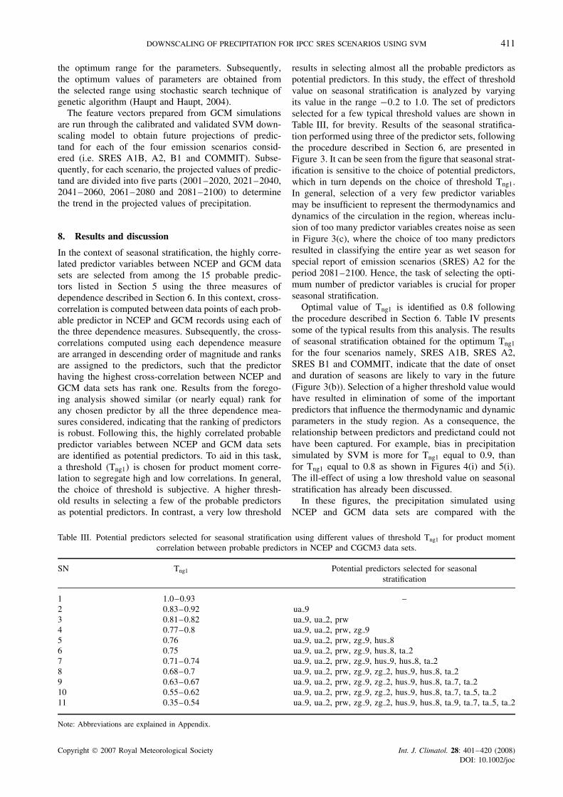
results in selecting almost all the probable predictors aspotential predictors. In this study, the effect of thresholdvalue on seasonal stratification is analyzed by varyingits value in the range −0.2 to 1.0. The set of predictorsselected for a few typical threshold values are shown inTable III, for brevity. Results of the seasonal stratifica-tion performed using three of the predictor sets, followingthe procedure described in Section 6, are presented inFigure 3. It can be seen from the figure that seasonal strat-ification is sensitive to the choice of potential predictors,which in turn depends on the choice of threshold Tng1.In general, selection of a very few predictor variablesmay be insufficient to represent the thermodynamics anddynamics of the circulation in the region, whereas inclu-sion of too many predictor variables creates noise as seenin Figure 3(c), where the choice of too many predictorsresulted in classifying the entire year as wet season forspecial report of emission scenarios (SRES) A2 for theperiod 2081–2100. Hence, the task of selecting the opti-mum number of predictor variables is crucial for properseasonal stratification.

Optimal value of Tng1 is identified as 0.8 followingthe procedure described in Section 6. Table IV presentssome of the typical results from this analysis. The resultsof seasonal stratification obtained for the optimum Tng1

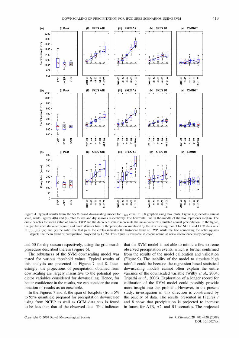
for the four scenarios namely, SRES A1B, SRES A2,SRES B1 and COMMIT, indicate that the date of onsetand duration of seasons are likely to vary in the future(Figure 3(b)). Selection of a higher threshold value wouldhave resulted in elimination of some of the importantpredictors that influence the thermodynamic and dynamicparameters in the study region. As a consequence, therelationship between predictors and predictand could nothave been captured. For example, bias in precipitationsimulated by SVM is more for Tng1 equal to 0.9, thanfor Tng1 equal to 0.8 as shown in Figures 4(i) and 5(i).The ill-effect of using a low threshold value on seasonalstratification has already been discussed.

In these figures, the precipitation simulated usingNCEP and GCM data sets are compared with the

Table III. Potential predictors selected for seasonal stratification using different values of threshold Tng1 for product momentcorrelation between probable predictors in NCEP and CGCM3 data sets.

SN Tng1 Potential predictors selected for seasonalstratification

1 1.0–0.93 –2 0.83–0.92 ua 93 0.81–0.82 ua 9, ua 2, prw4 0.77–0.8 ua 9, ua 2, prw, zg 95 0.76 ua 9, ua 2, prw, zg 9, hus 86 0.75 ua 9, ua 2, prw, zg 9, hus 8, ta 27 0.71–0.74 ua 9, ua 2, prw, zg 9, hus 9, hus 8, ta 28 0.68–0.7 ua 9, ua 2, prw, zg 9, zg 2, hus 9, hus 8, ta 29 0.63–0.67 ua 9, ua 2, prw, zg 9, zg 2, hus 9, hus 8, ta 7, ta 210 0.55–0.62 ua 9, ua 2, prw, zg 9, zg 2, hus 9, hus 8, ta 7, ta 5, ta 211 0.35–0.54 ua 9, ua 2, prw, zg 9, zg 2, hus 9, hus 8, ta 9, ta 7, ta 5, ta 2

Note: Abbreviations are explained in Appendix.



Figure 3. Typical results of seasonal stratification performed using cluster analysis. Dry season is shown in black color, whereas the wet seasonis shown in white color. The Tng1 values chosen are 0.9, 0.8 and 0.45 in Figure 3 (a)–(c) respectively.

Table IV. Selection of optimal value for threshold (Tng1)

between predictors in NCEP and GCM data sets. TL refers totruncation level expressed as percentage of TWP for the studyregion or as mean monthly Actual Evapotranspiration (MME).

Variable TL Tng1

0.9 0.8

TWP 0.70 0.70 0.750.75 0.70 0.760.80 0.70 0.760.85 0.70 0.780.90 0.71 0.780.95 0.71 0.781.00 0.72 0.77

MME – 0.64 0.67

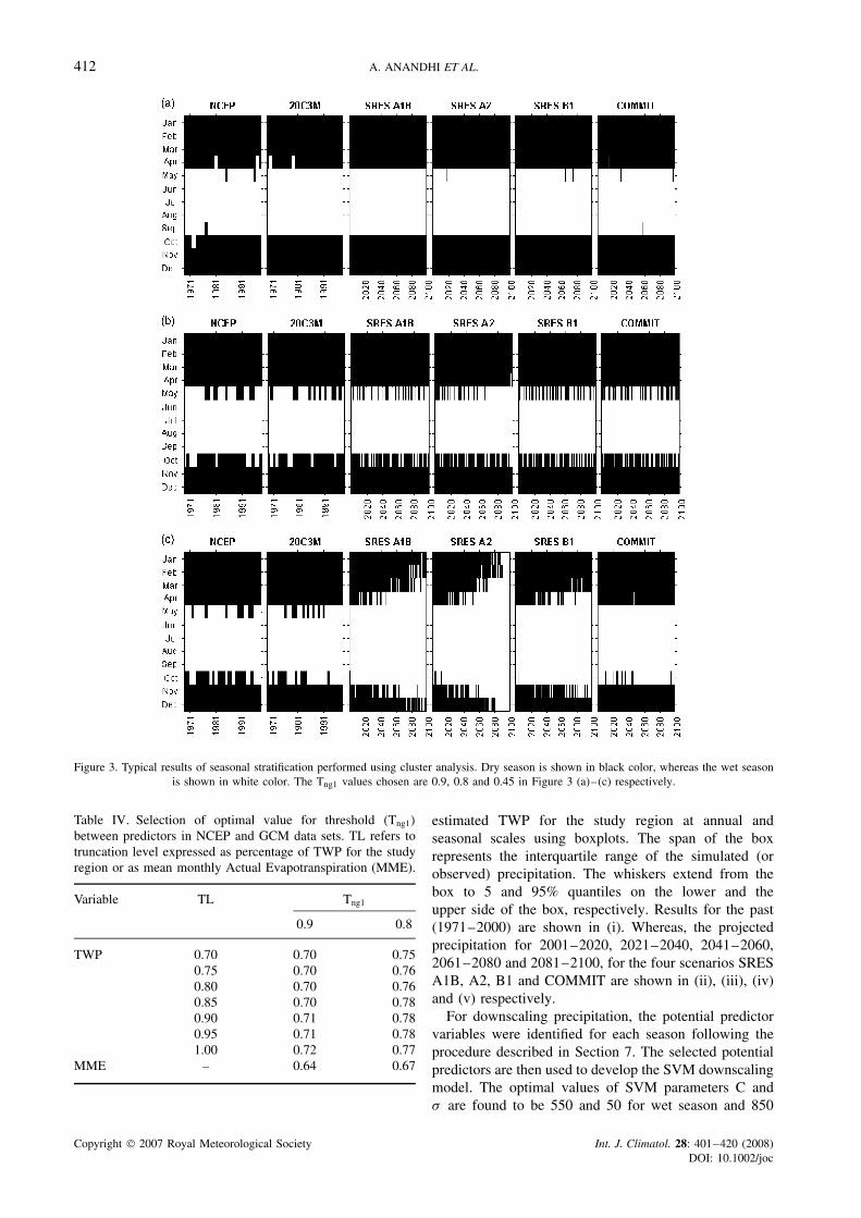
estimated TWP for the study region at annual andseasonal scales using boxplots. The span of the boxrepresents the interquartile range of the simulated (orobserved) precipitation. The whiskers extend from thebox to 5 and 95% quantiles on the lower and theupper side of the box, respectively. Results for the past(1971–2000) are shown in (i). Whereas, the projectedprecipitation for 2001–2020, 2021–2040, 2041–2060,2061–2080 and 2081–2100, for the four scenarios SRESA1B, A2, B1 and COMMIT are shown in (ii), (iii), (iv)and (v) respectively.

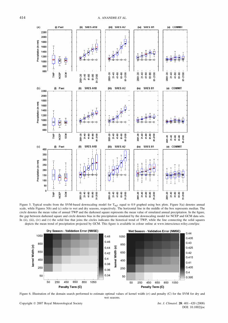
For downscaling precipitation, the potential predictorvariables were identified for each season following theprocedure described in Section 7. The selected potentialpredictors are then used to develop the SVM downscalingmodel. The optimal values of SVM parameters C andσ are found to be 550 and 50 for wet season and 850



Figure 4. Typical results from the SVM-based downscaling model for Tng1 equal to 0.8 graphed using box plots. Figure 4(a) denotes annualscale, while Figures 4(b) and (c) refer to wet and dry seasons respectively. The horizontal line in the middle of the box represents median. Thecircle denotes the mean value of annual TWP and the darkened square represents the mean value of simulated annual precipitation. In the figure,the gap between darkened square and circle denotes bias in the precipitation simulated by the downscaling model for NCEP and GCM data sets.In (ii), (iii), (iv) and (v) the solid line that joins the circles indicates the historical trend of TWP, while the line connecting the solid squares

depicts the mean trend of precipitation projected by GCM. This figure is available in colour online at www.interscience.wiley.com/ijoc

and 50 for dry season respectively, using the grid searchprocedure described therein (Figure 6).

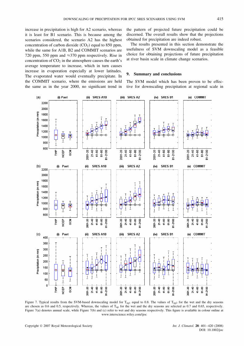
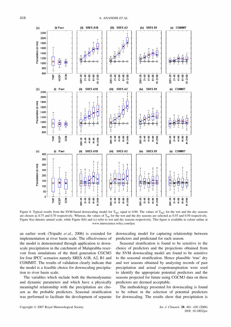
The robustness of the SVM downscaling model wastested for various threshold values. Typical results ofthis analysis are presented in Figures 7 and 8. Inter-estingly, the projections of precipitation obtained fromdownscaling are largely insensitive to the potential pre-dictor variables considered for downscaling. Hence, forbetter confidence in the results, we can consider the com-bination of results as an ensemble.

In the Figures 7 and 8, the span of boxplots (from 5%to 95% quantiles) prepared for precipitation downscaledusing from NCEP as well as GCM data sets is foundto be less than that of the observed data. This indicates

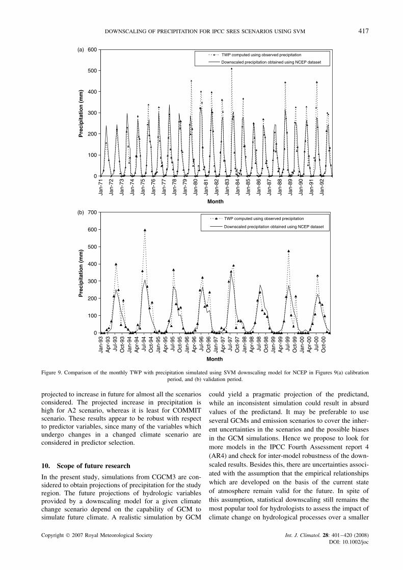
that the SVM model is not able to mimic a few extremeobserved precipitation events, which is further confirmedfrom the results of the model calibration and validation(Figure 9). The inability of the model to simulate highrainfall could be because the regression-based statisticaldownscaling models cannot often explain the entirevariance of the downscaled variable (Wilby et al., 2004;Tripathi et al., 2006). Exploration of a longer record forcalibration of the SVM model could possibly providemore insight into this problem. However, in the presentstudy, investigation in this direction is constrained bythe paucity of data. The results presented in Figures 7and 8 show that precipitation is projected to increasein future for A1B, A2, and B1 scenarios. The projected



Figure 5. Typical results from the SVM-based downscaling model for Tng1 equal to 0.9 graphed using box plots. Figure 5(a) denotes annualscale, while Figures 5(b) and (c) refer to wet and dry seasons, respectively. The horizontal line in the middle of the box represents median. Thecircle denotes the mean value of annual TWP and the darkened square represents the mean value of simulated annual precipitation. In the figure,the gap between darkened square and circle denotes bias in the precipitation simulated by the downscaling model for NCEP and GCM data sets.In (ii), (iii), (iv) and (v) the solid line that joins the circles indicates the historical trend of TWP, while the line connecting the solid squares

depicts the mean trend of precipitation projected by GCM. This figure is available in colour online at www.interscience.wiley.com/ijoc

Figure 6. Illustration of the domain search performed to estimate optimal values of kernel width (σ ) and penalty (C) for the SVM for dry andwet seasons.



increase in precipitation is high for A2 scenario, whereasit is least for B1 scenario. This is because among thescenarios considered, the scenario A2 has the highestconcentration of carbon dioxide (CO2) equal to 850 ppm,while the same for A1B, B2 and COMMIT scenarios are720 ppm, 550 ppm and ≈370 ppm respectively. Rise inconcentration of CO2 in the atmosphere causes the earth’saverage temperature to increase, which in turn causesincrease in evaporation especially at lower latitudes.The evaporated water would eventually precipitate. Inthe COMMIT scenario, where the emissions are heldthe same as in the year 2000, no significant trend in

the pattern of projected future precipitation could bediscerned. The overall results show that the projectionsobtained for precipitation are indeed robust.

The results presented in this section demonstrate theusefulness of SVM downscaling model as a feasiblechoice for obtaining projections of future precipitationat river basin scale in climate change scenarios.

9. Summary and conclusions

The SVM model which has been proven to be effec-tive for downscaling precipitation at regional scale in

Figure 7. Typical results from the SVM-based downscaling model for Tng1 equal to 0.8. The values of Tng2 for the wet and the dry seasonsare chosen as 0.6 and 0.5, respectively. Whereas, the values of Tnp for the wet and the dry seasons are selected as 0.7 and 0.65, respectively.Figure 7(a) denotes annual scale, while Figure 7(b) and (c) refer to wet and dry seasons respectively. This figure is available in colour online at

www.interscience.wiley.com/ijoc



Figure 8. Typical results from the SVM-based downscaling model for Tng1 equal to 0.80. The values of Tng2 for the wet and the dry seasonsare chosen as 0.75 and 0.70 respectively. Whereas, the values of Tnp for the wet and the dry seasons are selected as 0.55 and 0.50 respectively.Figure 8(a) denotes annual scale, while Figure 8(b) and (c) refer to wet and dry seasons respectively. This figure is available in colour online at

www.interscience.wiley.com/ijoc

an earlier work (Tripathi et al., 2006) is extended forimplementation at river basin scale. The effectiveness ofthe model is demonstrated through application to down-scale precipitation in the catchment of Malaprabha reser-voir from simulations of the third generation CGCM3for four IPCC scenarios namely SRES A1B, A2, B1 andCOMMIT. The results of validation clearly indicate thatthe model is a feasible choice for downscaling precipita-tion to river basin scale.

The variables which include both the thermodynamicand dynamic parameters and which have a physicallymeaningful relationship with the precipitation are cho-sen as the probable predictors. Seasonal stratificationwas performed to facilitate the development of separate

downscaling model for capturing relationship betweenpredictors and predictand for each season.

Seasonal stratification is found to be sensitive to thechoice of predictors and the projections obtained fromthe SVM downscaling model are found to be sensitiveto the seasonal stratification. Hence plausible ‘true’ dryand wet seasons obtained by analyzing records of pastprecipitation and actual evapotranspiration were usedto identify the appropriate potential predictors and theseasons projected for future using CGCM3 data on thesepredictors are deemed acceptable.

The methodology presented for downscaling is foundto be robust in the selection of potential predictorsfor downscaling. The results show that precipitation is



0

100

200

300

400

500

600

Jan-

71

Jan-

72

Jan-

73

Jan-

74

Jan-

75

Jan-

76

Jan-

77

Jan-

78

Jan-

79

Jan-

80

Jan-

81

Jan-

82

Jan-

83

Jan-

84

Jan-

85

Jan-

86

Jan-

87

Jan-

88

Jan-

89

Jan-

90

Jan-

91

Jan-

92

Month

Pre

cip

itat

ion

(m

m)

TWP computed using observed precipitation

Downscaled precipitation obtained using NCEP dataset

0

100

200

300

400

500

600

700

Jan-

93A

pr-9

3Ju

l-93

Oct

-93

Jan-

94A

pr-9

4Ju

l-94

Oct

-94

Jan-

95A

pr-9

5Ju

l-95

Oct

-95

Jan-

96A

pr-9

6Ju

l-96

Oct

-96

Jan-

97A

pr-9

7Ju

l-97

Oct

-97

Jan-

98A

pr-9

8Ju

l-98

Oct

-98

Jan-

99A

pr-9

9Ju

l-99

Oct

-99

Jan-

00A

pr-0

0Ju

l-00

Oct

-00

Month

Pre

cip

itat

ion

(m

m)

TWP computed using observed precipitation

Downscaled precipitation obtained using NCEP dataset

(a)

(b)

Figure 9. Comparison of the monthly TWP with precipitation simulated using SVM downscaling model for NCEP in Figures 9(a) calibrationperiod, and (b) validation period.

projected to increase in future for almost all the scenariosconsidered. The projected increase in precipitation ishigh for A2 scenario, whereas it is least for COMMITscenario. These results appear to be robust with respectto predictor variables, since many of the variables whichundergo changes in a changed climate scenario areconsidered in predictor selection.

10. Scope of future research

In the present study, simulations from CGCM3 are con-sidered to obtain projections of precipitation for the studyregion. The future projections of hydrologic variablesprovided by a downscaling model for a given climatechange scenario depend on the capability of GCM tosimulate future climate. A realistic simulation by GCM

could yield a pragmatic projection of the predictand,while an inconsistent simulation could result in absurdvalues of the predictand. It may be preferable to useseveral GCMs and emission scenarios to cover the inher-ent uncertainties in the scenarios and the possible biasesin the GCM simulations. Hence we propose to look formore models in the IPCC Fourth Assessment report 4(AR4) and check for inter-model robustness of the down-scaled results. Besides this, there are uncertainties associ-ated with the assumption that the empirical relationshipswhich are developed on the basis of the current stateof atmosphere remain valid for the future. In spite ofthis assumption, statistical downscaling still remains themost popular tool for hydrologists to assess the impact ofclimate change on hydrological processes over a smaller



region because its computational overheads are practi-cally insignificant compared to dynamic downscaling.

Several avenues can be explored to further refine thisattempt to statistically downscale GCM simulations. Thisproposed approach to statistical downscaling of precipita-tion is planned to be extended to five other cardinal vari-ables namely, maximum and minimum temperature, windspeed, relative humidity and solar radiation. Extendedresearch work in this direction is underway.

Acknowledgement

This work is partially supported by INCOH, Ministryof Water Resources, Govt. of India, through project no.23/52/2006-R&D. The authors express their gratitudeto the two anonymous reviewers for their constructivecomments and suggestions on the earlier draft of thepaper. Special thanks are also due to our alumnus MrShivam and Ms.Vidyunmala, Indian Institute of Science,Bangalore, for their valuable inputs.

Appendix: Abbreviations

Abbreviations used in text

CCCma Canadian Center for Climate Modelingand Analysis

CGCM3 Third generation Canadian GeneralCirculation Model

GCM General Circulation ModelIPCC Intergovernmental Panel on Climate

ChangeLS-SVM Least Square-Support Vector MachineMMP mean monthly precipitationNMSE Normalized mean square errorPCA Principal component analysisPC Principal componentRBF Radial basis functionSRES Special report of Emission scenariosSVM Support Vector MachineTL truncation levelTWP Thiessen Weighted precipitation

Abbreviations used in Tables I and III

Predictor Names

afs Airflow strengthBRN Bulk Richardson numberCAPE Convective Available Potential EnergyCI Convective inhibitionF Geostropic airflowhus specific humiditypr precipitationprw precipitable water contentps pressurerh relative humidity

SWTI Severe weather threat indexta air temperatureua zonal windva meridional windwa vertical windwd wind directionWS wind shearW wind speedzg geopotential heightzgt geopotential height thicknessZ vorticity

Measurement Height of Predictors

0 pressure height at 1000mb2 pressure heights at 200mb2m 2m from surface5 pressure height at 500mb7 pressure height at 700mb8 pressure height at 850mb9 pressure height at 925mbns near surfaces surface

Techniques

AM Analogue MethodCCA Canonical Correlation AnalysisEOF Empirical Orthogonal FunctionLS Local scalingMLP Multilayer perceptronPCA Principal Component AnalysisRNN Recurrent Neural NetworkSDSM Statisitical downscaling modelSOM Self Organizing MapsSVDA Singular value decomposition analysisTNN Temporal Neural Network

Data Source

BMRC Bureau of Meteorology Research CenterCGCM Canadian General Circulation ModelCSIRO Commonwealth Scientific and Industrial

Research OrganizationECMWF European Center for Medium-Range

Weather ForecastsHadAM Hadley center Atmosphere ModelLMD Laboratoire de Meteorologie Dynamique du.

References

Adams RM, Hurd BH, Lenhart S, Leary N. 1998. Effects of globalclimate change on agriculture: an interpretive review. ClimateResearch 11: 19–30.

Allen DM, Scibek J. 2006. Comparing modelled responses of two high-permeability unconfined aquifers to predicted climate change. Globaland Planetary Change (Netherlands) 50(1–2): 50–62.

Bardossy A, Bogardi I, Matyasovszky I. 2005. Fuzzy rule-baseddownscaling of precipitation. Theoretical and Applied Climatology82: 116–119.



Benestad RE, Hanssen-Bauer I, Førland EJ. 2007. An evaluation ofstatistical models for downscaling precipitation and their ability tocapture long-term trends. International Journal of Climatology 27(5):649–655.

Bergant K, Kajfez-Bogataj L. 2005. N-PLS regression as empiricaldownscaling tool in climate change studies. Theoretical and AppliedClimatology 81: 11–23.

Brotton J, Wall G. 1997. Climate change and the Bathurst caribou herdin the Northwest Territories Canada. Climatic Change 35: 35–52.

Burger G, Chen Y. 2005. Regression-based downscaling of spatialvariability for hydrologic applications. Journal of Hydrology 96:299–317.

Carter TR, La Rovere EL, Jones RN, Leemans R, Mearns LO, Naki-cenovic N, Pittock AB, Semenov SM, Skea J. 2001. Developing andapplying scenarios. Climate Change 2001: Impacts Adaptation andVulnerability. Cambridge University Press: Cambridge.

Cavazos T, Hewitson BC. 2005. Performance of NCEP variables instatistical downscaling of daily precipitation. Climate Research 28:95–107.

Cohen SJ, Miller KA, Hamlet AF, Avis W. 2000. Climate changeand resource management in the Columbia River basin. WaterInternational 25(2): 253–272.

Coughenour MB, Chen DX. 1997. Assessment of grassland ecosystemresponses to atmospheric change using plant-soil process models.Ecological Applications 7: 802–827.

Courant R, Hilbert D. 1970. Methods of Mathematical Physics, Vol. Iand II. Wiley Interscience: New York.

Crane RG, Hewitson BC. 1998. Doubled CO2 precipitation changesfor the Susquehanna basin: down-scaling from the genesis generalcirculation model. International Journal of Climatology 18: 65–76.

Darwin RF, Tsigas M, Lewandrowski J, Raneses A. 1995. Worldagriculture and climate change. Economic Adaptations AgriculturalEconomic Report Number 703. US Department of AgricultureEconomic Research Service: Washington, DC.

Dibike YB, Coulibaly P. 2005. Hydrologic impact of climate changein the Saguenay watershed: comparison of downscaling methods andhydrologic models. Journal of Hydrology 307: 145–163.

Dibike YB, Coulibaly P. 2006. Temporal neural networks fordownscaling climate variability and extremes. Neural Networks19(2): 135–144.

Doty B, Kinter JL III. 1993. The Grid Analysis and Display System(GrADS): a desktop tool for earth science visualization. In AmericanGeophysical Union 1993 Fall Meeting , San Fransico, CA, 6–10December.

Ferguson MAD. 1999. Arctic tundra caribou and climatic change:questions of temporal and spatial scales. Geoscience Canada 23:245–252.

Fix E, Hodges JL. 1951. Discriminatory analysis: nonparametricdiscrimination: consistency properties. Report. 4, Project 21-49-004,USAF School of Aviation Medicine.

Gestel TV, Suykens JAK, Baesens B, Viaene S, Vanthienen J,Dedene G, Moor BD, Vandewalle J. 2004. Benchmarking leastsquares support vector machine classifiers. Machine Learning 54(1):5–32.

Gosain AK, Sandhya R, Debajit B. 2006. Climate change impactassessment on hydrology of Indian river basins Special Section:Climate Change and India. Current Science 90(3): 346–353.

Gregory P, Ingram J, Campbell B, Goudriaan J, Hunt T, Landsberg J,Linder S, Stafford-Smith M, Sutherst B, Valentin C. 1999. Managedproduction systems. The Terrestrial Biosphere and Global ChangeImplications for Natural and Managed Ecosystems. CambridgeUniversity Press: Cambridge.

Hamilton LS. 1995. Mountain cloud forest conservation and research:a synopsis. Mountain Research and Development 15: 259–266.

Haupt RL, Haupt SE. 2004. Practical Genetic Algorithm. John Wileyand Sons: New Jersey.

Haylock MR, Cawley GC, Harpham C, Wilby RL, Goodess C. 2006.Downscaling heavy precipitation over the United Kingdom: acomparison of dynamical and statistical methods and their futurescenarios. International Journal of Climatology 26: 1397–1415,DOI: 10.1002/joc.1318.

Haykin S. 2003. Neural Networks: A Comprehensive Foundation,Fourth Indian Reprint. Pearson Education: Singapore.

Hewitson BC, Crane RG. 1996. Climate downscaling: techniques andapplication. Climate Research 7: 85–95.

Hewitson BC, Crane RG. 2006. Consensus between GCM climatechange projections with empirical downscaling: precipitationdownscaling over South Africa. International Journal of Climatology26: 1315–1337, DOI: 10.1002/joc.1314.

Houghton JT, Ding Y, Griggs DJ, Noguer M, van der Linden PJ,Dai X, Maskell K, Johnson CA. 2001. Climate Change 2001: TheScientific Basis. Cambridge University Press: Cambridge (UK) andNew York (USA).

Hush DR, Horne BG. 1993. Progress in supervised neural networks:what’s new since Lippmann? IEEE Signal Processing Magazine 10:8–39.

IPCC. 2001. Climate Change 2001: The Scientific Basis Contributionsof Working Group I to the Third Assessment Report of theInternational Panel on Climate Change. Cambridge University Press:Cambridge.

Jones MB, Jongen M. 1996. Sensitivity of temperate grassland speciesto elevated atmospheric CO2 and the interaction with temperatureand water stress. Agricultural and Food Science in Finland 5:271–283.

Kabat P, van Schaik SH. 2003. Climate changes the water rules:how water managers can cope with today’s climate variabilityand tomorrow’s climate change Dialogue on Water and ClimateNetherlands , Available from: 〈www.waterandclimate.org〉.

Kalnay E, Kanamitsu M, Kistler R, Collins W, Deaven D, Gandin L,Iredell M, Saha S, White G, Woollen J, Zhu Y, Chelliah M,Ebisuzaki W, Higgins W, Janowiak J, Mo KC, Ropelewski C,Wang J, Leetmaa A, Reynolds R, Jenne R, Joseph D. 1996. TheNCEP/NCAR 40-year reanalysis project. Bulletin of the AmericanMeteorological Society 77(3): 437–471.

Karl TR, Wang WC, Schlesinger ME, Knight RW, Portman D. 1990.A method of relating general circulation model simulated climateto the observed local climate Part I: Seasonal statistics. Journal ofClimate 3: 1053–1079.

Kendall MG. 1951. Regression structure and functional relationshippart I. Biometrika 38: 11–25.

Keerthi SS, Lin CJ. 2003. Asymptotic behaviors of support vectormachines with Gaussian kernel. Neural Computation 15(7):1667–1689.

Kim MK, Kang IS, Park CK, Kim KM. 2004. Super ensembleprediction of regional precipitation over Korea. International Journalof Climatology 24: 777–790.

Kirilenko AP, Solomon AM. 1998. Modeling dynamic vegetationresponse to rapid climate change using bioclimatic classification.Climatic Change 38: 15–49.

Krasovskaia I. 1995. Quantification of the stability of river flowregimes. Hydrological Sciences Journal 40: 587–598.

Lal M, Cubasch U, Voss R, Waszkewitz J. 1995. Effect of transientincrease in greenhouse gases and sulfate aerosols on monsoonclimate. Current Science 69: 752–763.

Leach C. 1979. Introduction to Statistics: A Nonparametric Approachfor the Social Sciences. Wiley: New York.

Lin HT, Lin CJ. 2003. A study on sigmoid kernels for SVM and thetraining of non-PSD kernels by SMO-type methods. Technical report.Department of Computer Science and Information Engineering,National Taiwan University.

Linz H, Shiklomanov I, Mostefakara K. 1990. Chapter 4 Hydrologyand water Likely impact of climate change, IPCC WGII reportWMO/UNEP, Geneva.

MacQueen J. 1967. Some methods for classification and analysisof multivariate observation. In Proceedings of the Fifth BerkeleySymposium on Mathematical Statistics and Probability, Vol. 1, LeCam LM, Neyman J (eds). University of California Press: Berkeley;281–297.

Maheras P, Tolika K, Anagnostopoulou C, Vafiadis M, Patrikas I,Flocas H. 2004. On the relationships between circulation types andchanges in rainfall variability in Greece. International Journal ofClimatology 24: 1695–1712.

Menzel L, Thieken A, Schwandt D, Burger G. 2006. Impact of climatechange on the regional hydrology – scenario-based modeling studiesin the German Rhine catchment. Natural Hazards 38(1–2): 45–61.

Mercer J. 1909. Functions of positive and negative type and theirconnection with the theory of integral equations. PhilosophicalTransactions of the Royal Society, London 209: 415–446.

Miller JR, Dixon MD, Turner MG. 2004. Response of aviancommunities in large-river floodplains to environmental variation atmultiple scales. Ecological Applications 14: 1394–1410.

Mirza MQ, Warrick RA, Ericksen NJ, Kenny GJ. 1998. Trends andpersistence in precipitation in the Ganges Brahmaputra and MeghnaBasins in South Asia. Hydrological Sciences Journal 43: 845–858.

More G. 1988. Impact of climate change and variability on recre-ation in the prairie provinces. In The Impact of ClimateVariability



and Change on the Canadian Prairies: Proceedings of the Sympo-sium/Workshop Edmonton Alberta Alberta, Canada, September 9–111987.

Nishiyama K, Ishikawa I, Jinno K, Kawamura A, Wakimizu K. 2002.Radar and GPV-based consideration on significant indices fordetecting heavy rainfall. In Proceedings of ERAD CopernicusGmbH ; Delft, The Netherlands, 272–276.

Nykanen DK, Foufoula-Georgiou E, Lapenta WM. 2001. Impact ofsmall-scale rainfall variability on larger-scale spatial organization ofland–atmosphere fluxes. Journal of Hydrometeorology 2: 105–120,DOI: 10.1175/1525-7541(2001)002.

Pearson K. 1896. Mathematical contributions to the theory of evolutionIII regression heredity and panmixia. Philosophical Transactions ofthe Royal Society of London Series 187: 253–318.

Perica S, Foufoula-Georgiou E. 1996. Linkage of scaling andthermodynamic parameters of rainfall: results from midlatitudemesoscale convective systems. Journal of Geophysical Research101(D3): 7431–7448, DOI: 10.1029/95JD02372.

Pounds JA, Fogden MPL, Campbell JH. 1999. Biological response toclimate change on a tropical mountain. Nature 398: 611–615.

Press WH, Teukolsky SA, Vetterling WT, Flannery BP. 1992. Numer-ical Recipes in Fortran 77: The Art of Scientific Computing. Cam-bridge University Press: New York.

Reynard NS, Prudhomme C, Crooks SM. 1998. The potential impactsof climate change on the flood characteristics of a large catchmentin the UK. Proceedings of the Second International Conference onClimate and Water Espoo Finland August 1998. Helsinki Universityof Technology, Helsinki, Finland.

Risby JS, Entekhabi D. 1996. Observed Sacremento Basin streamflowresponse to precipitation and temperature changes and its relevanceto climate impact studies. Journal of Hydrology 184: 209–223.

Richardson R. 2003. The effects of climate change on mountaintourism: a contingent behavior methodology. In First InternationalConference on Climate Change and Tourism Djerba Tunisia 9-11Djerba, Tunisia.

Salathe EP. 2003. Comparison of various precipitation downscalingmethods for the simulation of streamflow in a rainshadow riverbasin. International Journal of Climatology 23(8): 887–901, DOI:10.1002/joc.922.

Salathe EP. 2005. Downscaling simulations of future global climatewith application to hydrologic modeling. International Journal ofClimatology 25: 419–436.

Sandstrom K. 1995. Modeling the effects of rainfall variability onground water recharge in semi-arid Tanzania. Nordic Hydrology 26:313–330.

Schmidli J, Christoph F, Pier LV. 2006. Downscaling from GCMprecipitation: a benchmark for dynamical and statistical downscalingmethods. International Journal of Climatology 26(5): 679–689.

Schoof JT, Pryor SC, Robeson SM. 2007. Downscaling dailymaximum and minimum temperatures in the midwestern USA: ahybrid empirical approach. International Journal of Climatology27(4): 439–454.

Selvaraju R. 2003. Impact of El-Nino–southern oscillation on Indianfoodgrain production. International Journal of Climatology 23:187–206.

Shongwe EM, Landman WA, Mason SJ. 2006. Performance ofrecalibration systems for GCM forecasts for Southern Africa.International Journal of Climatology 26: 1567–1585, DOI:10.1002/joc.1319.

Smola AJ, Scholkopf B, Muller KR. 1998. The connection betweenregularization operators and support vector kernels. Neural Networks11(4): 637–649.

Spearman CE. 1904a. General intelligence objectively determined andmeasured. American Journal of Psychology 5: 201–293.

Spearman CE. 1904b. Proof and measurement of association betweentwo things. American Journal of Psychology 15: 72–101.

Stehlik J, Bardossy A. 2002. Multivariate stochastic downscalingmodel for generating daily precipitation series based on atmosphericcirculation. Journal of Hydrology 256: 120–141.

Suresh KR, Mujumdar PP. 2004. A fuzzy risk approach for perfor-mance evaluation of an irrigation reservoir system. AgriculturalWater Management 69: 159–177.

Suykens JAK. 2001. Nonlinear modeling and support vector machines.In Proceeding of IEEE Instrumentation and Measurement TechnologyConference, Budapest, Hungary; 287–294.

Tatli H, Dalfes HN, Mentes S. 2004. A statistical downscaling methodfor monthly total precipitation over Turkey. International Journal ofClimatology 24(2): 161–180.

Timbal B, Dufour A, McAvaney A. 2003. An estimate of futureclimate change for western France using a statistical downscalingtechnique. Climate Dynamics 20: 807–823, DOI 10.1007/s00382-002-0298-9.

Tolika K, Maheras P, Flocas HA, Papadimitriou AA. 2006. Anevaluation of a general circulation model (GCM) and theNCEP–NCAR reanalysis data for winter precipitation in Greece.International Journal of Climatology 26: 1376–1385.

Tripathi S, Srinivas VV, Nanjundiah RS. 2006. Downscaling ofprecipitation for climate change scenarios: a support vector machineapproach. Journal of Hydrology DOI: 10.1016/j.jhydrol.2006.04.030.

Tyler MJ. 1994. Climatic change and its implications for the amphibianfauna. Transactions of the Royal Society of South Australia 118:53–57.

Valentin C. 1996. Soil erosion under global change. Global Change andTerrestrial Ecosystems. Cambridge University Press: Cambridge.

Vapnik VN. 1995. The Nature of Statistical Learning Theory. Springer:New York.

Vapnik VN. 1998. Statistical Learning Theory. Wiley: New York.Venugopal V, Foufoula-Georgiou E, Sapozhnikov V. 1999a. Evidence

of dynamic scaling in space-time rainfall. Journal of GeophysicalResearch 104(D24): 31599–31610, DOI: 10.1029/1999JD900437.

Venugopal V, Foufoula-Georgiou E, Sapozhnikov V. 1999b. A space-time downscaling model for rainfall. Journal of GeophysicalResearch 104(D16): 19705–19722, DOI: 10.1029/1999JD900338.

Vicente-Serrano SM, Lopez-Moreno JI. 2006. The influence ofatmospheric circulation at different spatial scales on winter droughtvariability through a Semi-Arid Climatic Gradient in NortheastSpain. International Journal of Climatology 26: 1427–1453.

Wamukonya N. 2003. Managing climate change: strategies forGovernments Private sector and consumers. In InternationalConference on Climate Change and Tourism Djerba Tunisia 9–11Djerba, Tunisia.

Wang YQ, Leung LR, McGregor JL, Lee DK, Wang WC, Ding YH,Kimura F. 2004. Regional climate modeling: progress, challenges,and prospects. Journal of the Meteorological society of Japan 82:1599–1628.

Wetterhall F, Halldin S, Xu CY. 2005. Statistical precipitationdownscaling in central Sweden with the analogue method. Journalof Hydrology 306: 136–174.

Wilby RL, Wigley TML. 2000. Precipitation predictors for downscal-ing: observed and general circulation model relationships. Interna-tional Journal of Climatology 20(6): 641–661.

Wilby RL, Dawson CW, Barrow EM. 2002. SDSM – a decisionsupport tool for the assessment of climate change impacts.Environmental Modeling & Software 17: 147–159.

Wilby RL, Charles SP, Zorita E, Timbal B, Whetton P, Mearns LO.2004. The guidelines for use of climate scenarios developedfrom statistical downscaling methods. Supporting material ofthe Intergovernmental Panel on Climate Change (IPCC), pre-pared on behalf of Task Group on Data and Scenario Sup-port for Impacts and Climate Analysis (TGICA), (http://ipcc-ddc.cru.uea.ac.uk/guidelines/StatDown Guide.pdf).

Winkler JA, Palutikof JP, Andresen JA, Goodess CM. 1997. Thesimulation of daily temperature time series from GCM output Part II:Sensitivity analysis of an empirical transfer function methodology.Journal of Climate 10(10): 2514–2532.

Xoplaki E, Gonzalez-Rouco JF, Luterbacher J, Wanner H. 2004. Wetseason Mediterranean precipitation variability: influence of large-scale dynamics and trends. Climate Dynamics 23: 63–78.

Yaning C, Kuniyoshi T, Changchun X, Yapeng C, Zongxue X. 2006.Regional climate change and its effects on river runoff in the Tarimbasin China. Hydrological Processes DOI: 101002/hyp6200.

Zhang XC. 2005. Spatial downscaling of global climate model outputfor site-speciftc assessment of crop production and soil erosion.Agricultural and Forest Meteorology 135: 215–229.


downscaling precipitation to river basin in india for ipcc sres scenarios using support vector...

Documents