UNSUPERVISED ASSET CLUSTERANALYSIS IMPLEMENTED WITH
PARALLEL GENETIC ALGORITHMSON THE NVIDIA CUDA PLATFORM
by
Dariusz CieslakiewiczA dissertation submitted to the Faculty of Science, University of the
Witwatersrand, Johannesburg, in fulfilment of the requirements for thedegree of Master of Science
in theFaculty of Science
School of Computational and Applied Mathematics
Johannesburg,March 11,2014
The financial assitance of the National Research Foundation (NRF) towards thisresearch is hereby acknowledged. Opinions expressed and conclusions arrived at, are
those of the author and are not necessarily attributed to the NRF.

Declaration of Authorship
I declare that this dissertation is my own, unaided work. It is being submitted for theDegree of Master of Science in the University of the Witwatersrand, Johannesburg. Ithas not been submitted before for any degree or examination in any other University.
(Signature of candidate)
day of 20
i
UNIVERSITY OF WITWATERSRAND
AbstractFaculty of Science
School of Computational and Applied Mathematics
Master of Science
by Dariusz Cieslakiewicz
During times of stock market turbulence and crises, monitoring the clustering behaviourof financial instruments allows one to better understand the behaviour of the stock mar-ket and the associated systemic risks. In the study undertaken, I apply an effective andperformant approach to classify data clusters in order to better understand correlationsbetween stocks. The novel methods aim to address the lack of effective algorithms todeal with high-performance cluster analysis in the context of large complex real-timelow-latency data-sets. I apply an efficient and novel data clustering approach, namelythe Giada and Marsili log-likelihood function derived from the Noh model and use a Par-allel Genetic Algorithm in order to isolate residual data clusters. Genetic Algorithms(GAs) are a very versatile methodology for scientific computing, while the applicationof Parallel Genetic Algorithms (PGAs) further increases the computational efficiency.They are an effective vehicle to mine data sets for information and traits. However,the traditional parallel computing environment can be expensive. I focused on adoptingNVIDIAs Compute Unified Device Architecture (CUDA) programming model in orderto develop a PGA framework for my computation solution, where I aim to efficientlyfilter out residual clusters. The results show that the application of the PGA withthe novel clustering function on the CUDA platform is quite effective to improve thecomputational efficiency of parallel data cluster analysis.

Dedicated to my son Marcel, my parents Waldemar and Urszulaand my brothers Tomasz and Marek
iii

Acknowledgements
First and foremost, I would like offer my sincere gratitude to Professor Ebrahim Momo-
niat for his continuous support. Further, I would like to thank my supervisor Dr Diane
Wilcox for the comments, remarks and engagement through the learning process of this
dissertation.
iv
Contents
Declaration of Authorship i
Abstract ii
Acknowledgements iv
List of Figures ix
List of Tables xi
Abbreviations xii
Symbols xiii
1 Introduction 11.1 Objectives . . . . . . . . . . . . . . . . . . . . . . . . . . . . . . . . . . . . 21.2 Rationale . . . . . . . . . . . . . . . . . . . . . . . . . . . . . . . . . . . . 21.3 Structure . . . . . . . . . . . . . . . . . . . . . . . . . . . . . . . . . . . . 3
2 Cluster Analysis 52.1 Introduction . . . . . . . . . . . . . . . . . . . . . . . . . . . . . . . . . . . 62.2 Measures of Similarity and Dissimilarity . . . . . . . . . . . . . . . . . . . 6
2.2.1 Distance measures . . . . . . . . . . . . . . . . . . . . . . . . . . . 62.2.2 Correlation measure . . . . . . . . . . . . . . . . . . . . . . . . . . 72.2.3 Ordinal Measures . . . . . . . . . . . . . . . . . . . . . . . . . . . . 82.2.4 Hierarchical clustering . . . . . . . . . . . . . . . . . . . . . . . . . 8
2.2.4.1 Nearest-neighbour clustering . . . . . . . . . . . . . . . . 92.2.4.2 Farthest-neighbour clustering . . . . . . . . . . . . . . . . 102.2.4.3 Ward’s Method . . . . . . . . . . . . . . . . . . . . . . . . 10
2.2.5 Center-Based Partitional Clustering . . . . . . . . . . . . . . . . . 102.2.5.1 K-means clustering . . . . . . . . . . . . . . . . . . . . . 11
2.3 Applicability of Cluster Analysis in the finance industry . . . . . . . . . . 122.4 Cluster analysis based on the Maximum Likelihood principle . . . . . . . 13
2.4.1 Giada and Marsili clustering technique . . . . . . . . . . . . . . . . 142.4.2 Search heuristic approach and rationale . . . . . . . . . . . . . . . 17
v
Contents vi
3 Genetic Algorithms 193.1 Genetic Algorithms: An Overview . . . . . . . . . . . . . . . . . . . . . . 19
3.1.1 Genetic Operators . . . . . . . . . . . . . . . . . . . . . . . . . . . 213.1.1.1 Selection . . . . . . . . . . . . . . . . . . . . . . . . . . . 21
Roulette Wheel Selection . . . . . . . . . . . . . . . . . . . 22Rank Selection . . . . . . . . . . . . . . . . . . . . . . . . . 22Tournament Selection . . . . . . . . . . . . . . . . . . . . . 23Random Selection . . . . . . . . . . . . . . . . . . . . . . . 23Stochastic Universal Sampling . . . . . . . . . . . . . . . . . 23
3.1.1.2 Crossover . . . . . . . . . . . . . . . . . . . . . . . . . . . 24Single Point Crossover . . . . . . . . . . . . . . . . . . . . . 24Two-Point Crossover . . . . . . . . . . . . . . . . . . . . . . 24Uniform Crossover . . . . . . . . . . . . . . . . . . . . . . . 25Shuffle Crossover . . . . . . . . . . . . . . . . . . . . . . . . 26
3.1.1.3 Mutation . . . . . . . . . . . . . . . . . . . . . . . . . . . 26Flipping . . . . . . . . . . . . . . . . . . . . . . . . . . . . . 26Interchanging . . . . . . . . . . . . . . . . . . . . . . . . . . 27Reversing . . . . . . . . . . . . . . . . . . . . . . . . . . . . 27Mutation Probability . . . . . . . . . . . . . . . . . . . . . . 27
3.1.1.4 Elitism . . . . . . . . . . . . . . . . . . . . . . . . . . . . 273.1.1.5 Replacement . . . . . . . . . . . . . . . . . . . . . . . . . 28
Random Replacement . . . . . . . . . . . . . . . . . . . . . 28Weak Parent Replacement . . . . . . . . . . . . . . . . . . . 29Both Parents Replacement . . . . . . . . . . . . . . . . . . . 29
3.1.1.6 Advantages of Genetic Algorithms . . . . . . . . . . . . . 293.1.2 Non-binary Encodings . . . . . . . . . . . . . . . . . . . . . . . . . 303.1.3 Knowledge Based Techniques . . . . . . . . . . . . . . . . . . . . . 31
3.2 Parallel Genetic Algorithms . . . . . . . . . . . . . . . . . . . . . . . . . . 323.2.1 Discretised Genetic Algorithms . . . . . . . . . . . . . . . . . . . . 323.2.2 Master-slave Parallelisation . . . . . . . . . . . . . . . . . . . . . . 333.2.3 Multiple-deme Parallelisation . . . . . . . . . . . . . . . . . . . . . 34
3.2.3.1 Model Parameters . . . . . . . . . . . . . . . . . . . . . . 353.2.3.2 Migration Topology . . . . . . . . . . . . . . . . . . . . . 363.2.3.3 Number of Islands . . . . . . . . . . . . . . . . . . . . . . 38
4 Computational Platform 394.1 Parallel computing . . . . . . . . . . . . . . . . . . . . . . . . . . . . . . . 39
4.1.1 Architectures . . . . . . . . . . . . . . . . . . . . . . . . . . . . . . 394.1.2 Parallel programming and design paradigms . . . . . . . . . . . . . 404.1.3 Rationale . . . . . . . . . . . . . . . . . . . . . . . . . . . . . . . . 41
4.2 GPU . . . . . . . . . . . . . . . . . . . . . . . . . . . . . . . . . . . . . . . 414.3 NVIDIA CUDA platform . . . . . . . . . . . . . . . . . . . . . . . . . . . 42
4.3.1 Execution Environment . . . . . . . . . . . . . . . . . . . . . . . . 434.3.2 Thread hierarchy . . . . . . . . . . . . . . . . . . . . . . . . . . . . 434.3.3 Memory hierarchy . . . . . . . . . . . . . . . . . . . . . . . . . . . 46
4.3.3.1 Registers . . . . . . . . . . . . . . . . . . . . . . . . . . . 464.3.3.2 Shared memory . . . . . . . . . . . . . . . . . . . . . . . 47
Contents vii
4.3.3.3 Global memory . . . . . . . . . . . . . . . . . . . . . . . . 484.3.4 Synchronisation . . . . . . . . . . . . . . . . . . . . . . . . . . . . . 48
4.3.4.1 CPU . . . . . . . . . . . . . . . . . . . . . . . . . . . . . 49CPU Explicit Synchronisation . . . . . . . . . . . . . . . . . 49CPU Implicit Synchronisation . . . . . . . . . . . . . . . . . 50
4.3.4.2 GPU . . . . . . . . . . . . . . . . . . . . . . . . . . . . . 50GPU simple synchronisation . . . . . . . . . . . . . . . . . . 51GPU tree-based synchronisation . . . . . . . . . . . . . . . 52GPU lock-free synchronization . . . . . . . . . . . . . . . . 52Disadvantages of GPU synchronisation . . . . . . . . . . . . 53
4.3.5 Challenges . . . . . . . . . . . . . . . . . . . . . . . . . . . . . . . 554.3.6 Performance tuning techniques . . . . . . . . . . . . . . . . . . . . 56
4.4 PGA implementations on GPUs . . . . . . . . . . . . . . . . . . . . . . . . 584.4.1 GAROP: Genetic Algorithms framework for Running On Parallel
environments . . . . . . . . . . . . . . . . . . . . . . . . . . . . . . 594.4.2 Hybrid Master-slave and Multiple-deme implementation on the
CUDA platform . . . . . . . . . . . . . . . . . . . . . . . . . . . . 61
5 Implementation 645.1 Stock correlation taxonomy . . . . . . . . . . . . . . . . . . . . . . . . . . 655.2 Approach . . . . . . . . . . . . . . . . . . . . . . . . . . . . . . . . . . . . 665.3 Pre-processing of data for the Clustering Algorithm . . . . . . . . . . . . 685.4 Post-processing of data and depiction of residual clusters . . . . . . . . . . 695.5 Implementation of a Parallel Genetic Algorithm: Master-Slave approach . 695.6 Detailed analysis of the Parallel Genetic Algorithm: Master-Slave approach 72
5.6.1 Data Parallelism . . . . . . . . . . . . . . . . . . . . . . . . . . . . 725.6.2 Initialisation . . . . . . . . . . . . . . . . . . . . . . . . . . . . . . 745.6.3 Grid, block and thread heuristics . . . . . . . . . . . . . . . . . . . 755.6.4 Master-slave GA computation parallelisation . . . . . . . . . . . . 755.6.5 Initial Population generation . . . . . . . . . . . . . . . . . . . . . 775.6.6 Evaluation of the fitness function . . . . . . . . . . . . . . . . . . . 785.6.7 Genetic Operators and Genetic Algorithm configuration . . . . . . 79
5.6.7.1 Scaling . . . . . . . . . . . . . . . . . . . . . . . . . . . . 805.6.7.2 Selection . . . . . . . . . . . . . . . . . . . . . . . . . . . 805.6.7.3 Crossover Operator . . . . . . . . . . . . . . . . . . . . . 815.6.7.4 Mutation Operator . . . . . . . . . . . . . . . . . . . . . 82
Creep mutation . . . . . . . . . . . . . . . . . . . . . . . . . 825.6.7.5 Random replacement . . . . . . . . . . . . . . . . . . . . 845.6.7.6 Replacement Operator . . . . . . . . . . . . . . . . . . . 84
5.6.8 Termination Criteria . . . . . . . . . . . . . . . . . . . . . . . . . . 855.7 Parallel Genetic Algorithm tuning . . . . . . . . . . . . . . . . . . . . . . 855.8 Measurement metrics . . . . . . . . . . . . . . . . . . . . . . . . . . . . . . 87
5.8.1 Performance metric . . . . . . . . . . . . . . . . . . . . . . . . . . 875.8.2 Average calculations . . . . . . . . . . . . . . . . . . . . . . . . . . 88
6 Experiments and Measurements 896.1 Environment . . . . . . . . . . . . . . . . . . . . . . . . . . . . . . . . . . 90
Contents viii
6.2 Data: Training Set . . . . . . . . . . . . . . . . . . . . . . . . . . . . . . . 916.2.1 Cluster Analysis in Matlab using a serial Genetic Algorithm . . . . 926.2.2 Experiments for tuning of parameters in Master-Slave PGA Algo-
rithm on the GPU . . . . . . . . . . . . . . . . . . . . . . . . . . . 936.2.2.1 Variation in Population Size . . . . . . . . . . . . . . . . 936.2.2.2 Variation in Crossover probability Pc . . . . . . . . . . . 966.2.2.3 Variation in Mutation probability Pm . . . . . . . . . . . 976.2.2.4 Variation in Knowledge-based crossover fragment opera-
tor probability Pcf . . . . . . . . . . . . . . . . . . . . . . 996.2.2.5 Variation in Crossover genetic operator . . . . . . . . . . 1006.2.2.6 Variation in Mutation genetic operator . . . . . . . . . . 1026.2.2.7 Variation in number of elite individuals promoted to the
next generation . . . . . . . . . . . . . . . . . . . . . . . 1046.3 Data: Intra-day stock prices for 18 stocks from the Johannesburg Stock
Exchange (JSE) . . . . . . . . . . . . . . . . . . . . . . . . . . . . . . . . . 1066.4 PGA algo execution time trials of the CUDA cluster analysis algorithm . 114
6.4.1 PGA algo execution time trials results . . . . . . . . . . . . . . . . 1146.4.2 Analysis of GA algo execution time trials . . . . . . . . . . . . . . 118
7 Conclusions and future prospects 1197.1 Conclusions . . . . . . . . . . . . . . . . . . . . . . . . . . . . . . . . . . . 1197.2 Future prospects . . . . . . . . . . . . . . . . . . . . . . . . . . . . . . . . 120
Bibliography 122
List of Figures
2.1 Hierarchical clustering . . . . . . . . . . . . . . . . . . . . . . . . . . . . . 9
3.1 Basic scheme of the Genetic Algorithm. . . . . . . . . . . . . . . . . . . . 203.2 Roulette Wheel Selection . . . . . . . . . . . . . . . . . . . . . . . . . . . 223.3 Stochastic Universal Sampling Approach . . . . . . . . . . . . . . . . . . . 243.4 Single Point Crossover Approach . . . . . . . . . . . . . . . . . . . . . . . 253.5 Two-Point Crossover Approach . . . . . . . . . . . . . . . . . . . . . . . . 253.6 Uniform Crossover Approach . . . . . . . . . . . . . . . . . . . . . . . . . 263.7 Flipping Approach . . . . . . . . . . . . . . . . . . . . . . . . . . . . . . . 273.8 Interchanging Approach . . . . . . . . . . . . . . . . . . . . . . . . . . . . 273.9 Schematic representation of migration topologies: A. Chain B. Uni-directional
ring C. Ring D. Ring + 1 + 2 E. Ring + 1 + 2 + 3 F. Torus G. CartwheelH. Lattice [1] . . . . . . . . . . . . . . . . . . . . . . . . . . . . . . . . . . 37
4.1 Three-Layered CUDA Application Architecture . . . . . . . . . . . . . . . 424.2 Serial-Parallel code invocation and execution on Host and Device . . . . . 444.3 Thread Hierarchy . . . . . . . . . . . . . . . . . . . . . . . . . . . . . . . . 454.4 Heterogeneous Programming model . . . . . . . . . . . . . . . . . . . . . . 474.5 CPU Explicit Synchronisation . . . . . . . . . . . . . . . . . . . . . . . . . 494.6 CPU Implicit Synchronisation . . . . . . . . . . . . . . . . . . . . . . . . . 504.7 GPU tree-based synchronisation . . . . . . . . . . . . . . . . . . . . . . . 524.8 Asynchronous and Sequential Data Transfers with Computations . . . . . 584.9 GAROP Architecture . . . . . . . . . . . . . . . . . . . . . . . . . . . . . 604.10 GAROP Architecture for the GPU . . . . . . . . . . . . . . . . . . . . . . 614.11 Hybrid PGA CUDA architecture . . . . . . . . . . . . . . . . . . . . . . . 62
5.1 A schematic depiction of a Master-slave PGA . . . . . . . . . . . . . . . . 715.2 Mapping of individuals onto the CUDA thread hierarchy . . . . . . . . . . 745.3 Stochastic uniform selection approach . . . . . . . . . . . . . . . . . . . . 81
6.1 Fitness vs. generation with the following GA configuration: 40x40 corre-lation matrix, 400 generations, a genome length of 40 and population sizeof 400, 100 stall generations and tolerance value of 0.001. . . . . . . . . . 92
6.2 Optimal cluster configuration of training set data obtained by Master-Slave PGA . . . . . . . . . . . . . . . . . . . . . . . . . . . . . . . . . . . 94
6.3 Variation in Population Size . . . . . . . . . . . . . . . . . . . . . . . . . . 956.4 Variation in Crossover probability Pc . . . . . . . . . . . . . . . . . . . . . 966.5 Variation in Mutation probability Pm . . . . . . . . . . . . . . . . . . . . 986.6 Variation in Knowledge-based crossover fragment operator probability Pcf 100
ix
List of Figures x
6.7 Variation in Crossover genetic operator . . . . . . . . . . . . . . . . . . . . 1016.8 Variation in Mutation genetic operator . . . . . . . . . . . . . . . . . . . . 1036.9 Variation in Number of elite individuals promoted to the next generation 1046.10 Early morning trading pattern on the 28th of September 2012 . . . . . . . 1076.11 Early morning trading pattern on on the 1st of October 2012 . . . . . . . 1086.12 Early morning trading pattern on the the 2nd of October 2012 . . . . . . 1096.13 Midday trading pattern snapshot on the 1st October 2012 . . . . . . . . . 1106.14 Midday trading pattern snapshot on the 2nd October 2012 . . . . . . . . 1116.15 Midday trading pattern snapshot on on 4th October 2012 . . . . . . . . . 1126.16 Afternoon trading pattern snapshot on the 1st October 2012 . . . . . . . 1136.17 Afternoon trading pattern snapshot on the 1st October 2012 . . . . . . . 1136.18 Afternoon trading pattern snapshot on the 3rd October 2012 . . . . . . . 1146.19 GA execution time runs in various execution environments . . . . . . . . . 1156.20 PGA execution time runs in various execution environments (Average
execution time recorded) . . . . . . . . . . . . . . . . . . . . . . . . . . . . 1156.21 PGA execution time runs in various execution environments (Maximum
execution time recorded) . . . . . . . . . . . . . . . . . . . . . . . . . . . . 1166.22 PGA execution time runs in various execution environments (Minimum
execution time recorded) . . . . . . . . . . . . . . . . . . . . . . . . . . . . 117
List of Tables
3.1 Migration Topology characteristics . . . . . . . . . . . . . . . . . . . . . . 36
4.1 NVIDIA GPU cards . . . . . . . . . . . . . . . . . . . . . . . . . . . . . . 55
6.1 Development and Testing environment . . . . . . . . . . . . . . . . . . . . 916.2 GA parameter configurations . . . . . . . . . . . . . . . . . . . . . . . . . 936.3 GA parameter configurations: Variation in Population Size . . . . . . . . 946.4 GA parameter configurations: Variation in Crossover probability Pc . . . 966.5 GA parameter configurations: Variation in Mutation probability Pm . . . 986.6 GA parameter configurations: Variation in Knowledge-based crossover
fragment operator probability Pcf . . . . . . . . . . . . . . . . . . . . . . . 996.7 GA parameter configurations: Variation in Crossover genetic operator . . 1016.8 GA parameter configurations: Variation in Mutation genetic operator . . 1026.9 GA parameter configurations: Variation in number of elite individuals
promoted to the next generation . . . . . . . . . . . . . . . . . . . . . . . 1046.10 Stocks traded on the Johannesburg Stock Exchange (JSE) . . . . . . . . . 106
xi
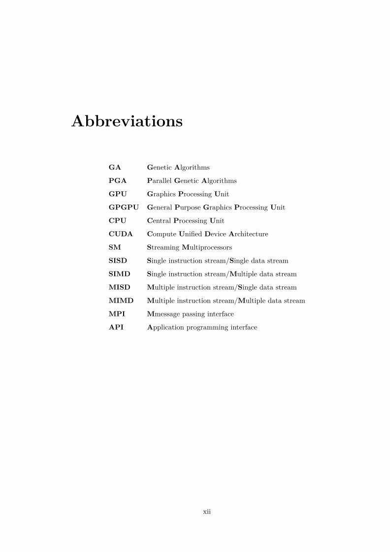
Abbreviations
GA Genetic Algorithms
PGA Parallel Genetic Algorithms
GPU Graphics Processing Unit
GPGPU General Purpose Graphics Processing Unit
CPU Central Processing Unit
CUDA Compute Unified Device Architecture
SM Streaming Multiprocessors
SISD Single instruction stream/Single data stream
SIMD Single instruction stream/Multiple data stream
MISD Multiple instruction stream/Single data stream
MIMD Multiple instruction stream/Multiple data stream
MPI Mmessage passing interface
API Application programming interface
xii
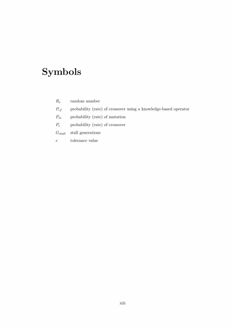
Symbols
Rc random number
Pcf probability (rate) of crossover using a knowledge-based operator
Pm probability (rate) of mutation
Pc probability (rate) of crossover
Gstall stall generations
e tolerance value
xiii
Chapter 1
Introduction
Cluster analysis is applied to financial time series data in order to identify securities
with related returns, so that one can diversify and thus optimise a financial portfolio[2].
Clustering is the process of grouping data into clusters so that objects within a cluster
have high similarity in comparison to one another, but are very dissimilar to objects in
other clusters[3]. In order to be able to filter through all the noise and isolate structures,
one needs to make use of a computational approach, that is well-suited to the traversal
of vast search spaces of data and the computation of classifications. Genetic algorithms
are such an approach. They are numerical optimisation algorithms inspired by natural
selection and genetics[4–6], that intelligently exploit a search space to solve optimisation
problems. Although the algorithms must traverse huge spaces, the computationally
intensive calculations can be performed independently[4–6]. The application of Parallel
Genetic Algorithms (PGAs) increases the computational efficiency and represents an
efficient vehicle for the mining of data-sets for information and traits[6]. PGAs paired
with a parallel computing environment allows for quick and effective computation[6].
Compute Unified Device Architecture (CUDA) is NVIDIA’s parallel computing platform
1
Chapter 1. Introduction 2
that enables enthusiasts and scientists to dramatically improve computing performance
by harnessing the power of the GPU[7–10].
1.1 Objectives
The main objective of this research was to develop a Master-slave Parallel Genetic Al-
gorithm (PGA) framework for unsupervised cluster analysis on the CUDA platform.
Master-slave PGAs, also denoted as Global PGAs, involve a single population, but dis-
tributed amongst multiple processing units for determination of fitness values and the
consequent application of genetic operators[6, 9, 10]. It must be able to isolate residual
clusters using the Giada and Marsili likelihood function[11]. The Giada and Marsili’s[11]
maximum log-likelihood function is used as a measure of the similarity of objects. It
is an unsupervised clustering function, meaning that the optimal number of clusters is
unknown a priori and thus not fixed at the beginning of the cluster analysis. Addition-
ally, I investigated and determined the most appropriate genetic operators in order to
maximise quality and performance of the proposed cluster analysis approach[11].
1.2 Rationale
This main focus of this research is to investigate the suitability of using the Giada and
Marsili log-likelihood function[11] with PGAs in a GPU parallel computing environment.
Examining the clustering behaviour of financial instruments, allows me to eliminate any
overlap in an investment portfolio by identifying securities with related returns. This
approach increases diversification. Diversification strives to smooth out unsystematic
risk events in a portfolio so that the positive performance of some investments will
Chapter 1. Introduction 3
neutralize the negative performance of others and in turn will reduce the inherent risk
on the portfolio[2].
1.3 Structure
A three-tiered approach was applied to investigate the suitability of using the Giada and
Marsili log-likelihood function[11] with PGAs in a GPU parallel computing environment.
The first tier of the thesis presents an up-to-date literature study on cluster analysis,
where the reader is familiarised with a Giada and Marsili log-likelihood function[11].
This thesis is the continuation of work done by Mbambiso[12], where he utilised a simu-
lated annealing optimisation approach using a maximum likelihood model developed by
Noh[13] in order to isolate an underlying structure of correlated asset returns, denoted
as sectors, and correlated market-wide activities, denoted as states in the SA financial
markets. In this research, a similar data clustering approach will be followed by us-
ing a Giada and Marsili’s[11] log-likelihood function, as a measure of the similarity of
objects, and thus clusters, but one will apply a more efficient search heuristic, namely
Genetic Algorithms. Artificial Intelligence search heuristic approaches, denoted Genetic
Algorithms, are introduced in order to to apply the cluster analysis function in an op-
timal and efficient manner, thus forming the second tier of the research. The focus
then shifts onto Parallel Genetic Algorithms in order to provide a computational ap-
proach to push the boundaries of computational performance. The third tier comprises
the vehicle for computation: the CUDA platform on General Purpose Graphics Pro-
cessing Units(GPGPUs). GPGPUs are commodity hardware, which have revolutionised
cutting-edge research into Parallel Computing. A closer look is taken at the implementa-
tion of Master-Slave Parallel Genetic Algorithm(PGA), with a detailed dissection of all
Chapter 1. Introduction 4
the approaches taken. The results section depicts the behaviour and intrinsic properties
of the algorithm and features a section on algorithm tuning for a training set of four
clusters. It includes a section on code execution times obtained, where Gebbie’s serial
GA implementation[12, 14] and the newly developed clustering implementation were run
on various Operating Systems, justifying the utilisation of GPUs and Parallel Genetic
Algorithms with the cluster analysis approach taken. The section is rounded off by the
application of the cluster analysis approach to real-world data. It features a clustering
analysis of 1780 time units of real-word stock prices taken from the JSE spanning over
the time period from 28th September 2012 until 10th of October 2012. A high-level
interpretation of trends observed for that specific time period is presented using Mul-
tiple Spanning Trees, which depict the correlations of the stock prices of assets under
investigation. The conclusion succinctly summarises the findings and presents further
prospects which might emanate from this research.
Chapter 2
Cluster Analysis
In the research undertaken, I undertake to find an effective and performant approach
to classify data clusters in order to better understand correlations between stocks. The
novel methods discussed here aim to address the lack of effective algorithms to deal with
high-performance cluster analysis in the context of large complex real-time low-latency
data-sets. I apply an efficient and novel data clustering approach, namely the Giada and
Marsili log-likelihood function[11] derived from the Noh model[13], to try to classify data
clusters. The chapter provides an overview of measures of similarity and dissimilarity
to provide a measure for the clusterability of data. I then look at areas of applicability
of cluster analysis, list the common types of clustering procedures and then provide
an in-depth analysis of the chosen clustering approach, namely the Giada and Marsili
log-likelihood function[11]. The research will be performed on normalised financial data,
meaning that the data will undergo preconditioning in order to remove outliers caused
by unusual or one-time influences. The data-set comprises stock returns, which consist
of the income and the capital gains relative on an investment in a particular stock asset.
5
Chapter 2. Cluster Analysis 6
2.1 Introduction
Cluster analysis divides data into groups, or clusters, which are meaningful, useful or
both. The goal is that the objects in a group will be similar or related to one other and
different from or unrelated to the objects in other groups. The greater the homogeneity
within a group, and the greater the heterogeneity between groups, the more pronounced
the clustering[3].
2.2 Measures of Similarity and Dissimilarity
There are various measures to express the similarity or dissimilarity between pairs of
objects.
2.2.1 Distance measures
The most commonly used proximity measure is the Minkowski metric, which is a gen-
eralization of the normal distance between points in Euclidean space[3]. It is defined
as
Pij = (d∑
k=1‖xik − xjk‖r)
1r (2.1)
where, r is a parameter, d is the dimensionality of the data object, and xik and xjk are,
respectively, the kth components of the ith and jth objects, xi and xj . Literature lists
the following Minkowski distances for specific values of r.[3]:
1. r = 1. City block or Taxicab distance, a common example being the Hamming
distance which measures the number of bits that are different in two binary vectors.
Chapter 2. Cluster Analysis 7
2. r = 2. The most common measure for the distance. This type of distance is
referred to as the Euclidean distance and is the most commonly used approach in
working with ratio or interval-scaled data.
3. r −→ ∞ .The supremum distance (Lmaxnorm,L∞), which denotes the maximum
difference between any component of the vectors.
The dimension d is combined with the respective Minkowski distance r to yield an overall
distance measure.
2.2.2 Correlation measure
The correlation measure is an approach to standardise data by using correlations, in
other words the statistical interdependence between data points. The correlation indi-
cates the direction and the degree of the relationship between two data points. The
direction of the relationship can either be positive or negative and if positive indicates
that the data points are in increasing positive relationship to each other, in other words
correlation, whilst if negative , in decreasing relationship to each other, denoted by the
term anti-correlation. The degree of the relationship measures the strength of the re-
lationship. The most common correlation coefficient which measures the relationship
between data points is the Pearson correlation coefficient, which is sensitive only to a
linear relationship between them. The Pearson correlation has a value of +1 in the
case of a perfect positive linear relationship and a value of −1 in the case of a perfect
decreasing linear relationship, and some value between −1 and 1 in all other cases, in-
dicating the degree of linear dependence between the variables. As it approaches zero
there is less of a relationship , meaning that there is a diminishing relationship or linear
Chapter 2. Cluster Analysis 8
interdependence between the points and the closer the coefficient is to either −1 or 1,
the stronger the correlation between the variables.
2.2.3 Ordinal Measures
Another type of proximity measure is derived by ranking the distances between pairs of
points from 1 to m * (m - 1) / 2. This type of measure can be used with most types of
data and is often used with a number of the hierarchical clustering, which is covered in
2.2.4.
2.2.4 Hierarchical clustering
[15] describes hierarchical clustering as procedures that are characterised by a tree-
like structure, a dendogram, which emerges in the course of the analysis. Clusters are
consecutively formed from objects. Initially, this type of procedure starts with each
object representing an individual cluster. These clusters are then sequentially merged
according to their similarity. First, the two most similar clusters , for example those
with the smallest distance between them, are merged to result in a new cluster at
the bottom of the hierarchy. This method builds the hierarchy from the individual
elements by progressively merging clusters and linking them to a higher level of the
hierarchy. This continues until a single, all inclusive cluster at the top and singleton
clusters of individual points at the bottom emerge. This allows a hierarchy of clusters
to be established from the bottom up. This category of hierarchical clustering is called
is agglomerative clustering. A cluster hierarchy can also be generated top-down, where
all objects are initially merged into a single cluster, which is then gradually split up
as I move down the hierarchy. In hierarchical clustering a cluster on a higher level
Chapter 2. Cluster Analysis 9
of the hierarchy always encompasses all clusters from a lower level. This means that
if an object is assigned to a certain cluster, there is no possibility of reassigning this
object to another cluster. This category of hierarchical clustering is called is divisive
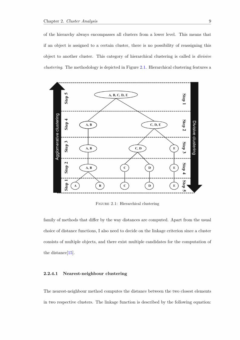
clustering. The methodology is depicted in Figure 2.1. Hierarchical clustering features a
Figure 2.1: Hierarchical clustering
family of methods that differ by the way distances are computed. Apart from the usual
choice of distance functions, I also need to decide on the linkage criterion since a cluster
consists of multiple objects, and there exist multiple candidates for the computation of
the distance[15].
2.2.4.1 Nearest-neighbour clustering
The nearest-neighbour method computes the distance between the two closest elements
in two respective clusters. The linkage function is described by the following equation:
Chapter 2. Cluster Analysis 10
D(x, y) = minx∈X,y∈Y
d(x, y) where X and Y are any two sets of data points considered as
clusters, and d(x, y) denotes the distance between the two elements x and y.
2.2.4.2 Farthest-neighbour clustering
The farthest-neighbour approach computes the maximum distance between a pair data
objects in respective clusters. D(x, y) = maxx∈X,y∈Y
(d(x, y)) where X and Y are any two
sets of data points considered as clusters, and d(x, y) denotes the distance between the
two elements x and y. This approach is an agglomerative procedure.
2.2.4.3 Ward’s Method
For Ward’s method the proximity between two clusters is defined as the increase in the
squared error that results when two clusters are merged. Thus, this method uses the
same objective function as is used by the K-means clustering. While it may seem that
this makes this technique somewhat distinct from other hierarchical techniques, some
algebra will show that this technique is very similar to the group average method when
the proximity between two points is taken to be the square of the distance between
them[15].
2.2.5 Center-Based Partitional Clustering
Another important group of clustering procedures are partitioning methods. As with
hierarchical clustering, there is a wide array of different algorithms; of these, the k-means
procedure and the k-mediod being the most recognised. The optimization problem
itself is known to be NP-hard, and thus the common approach is to search only for
approximate solutions. Both techniques are based on the notion that a center point
Chapter 2. Cluster Analysis 11
can represent a cluster. They distinguish themselves by the fact that K-means uses the
concept of a centroid, which is the median value of a group of points, which almost never
corresponds to an actual data point, whilst the K-medoid clustering approach utilises
the idea of determining a medoid, which is the most representative point of a group of
points.
2.2.5.1 K-means clustering
This algorithm uses the within-cluster variation as a measure of the homogeneity of a
cluster. The procedure aims at segmenting data in such a way that the variation of the
data points within a cluster is minimised. Prior to analysis, I have to decide on the
number of clusters. Based on this information, the algorithm randomly selects a center
for each cluster and the clustering process starts by randomly assigning objects to the
chosen number of clusters. I proceed then to re-allocate objects to other clusters in order
to reduce the within-cluster variation. Given a set of observations (x1, x2, ..., xn) , where
each observation is a d-dimensional real vector, k-means clustering aims to partition the
n observations into k sets S = (S1, S2, ..., Sk) so as to minimise the Euclidean distance,
that being the measure of proximity of the data point to the centroid of the cluster
denoted by
arg maxS
=k∑i=1
∑xj∈Si
‖xj − µi‖2 (2.2)
where µi is the mean of the points in Si. for every single object. Each object is then
assigned to the centroid with the shortest distance to it. I proceed in an iterative manner
until pre-defined termination criteria is reached, for example a predetermined number
of iterations or there is no change in cluster affiliations, meaning there is no change in
centroids.
Chapter 2. Cluster Analysis 12
2.3 Applicability of Cluster Analysis in the finance indus-
try
Conceptually meaningful groups of objects that share common characteristics, play an
important role in how people analyse and describe the world. The human mind divides
up objects into groups and assigning particular objects to these groups , by the process
of classification. In the context of understanding data, clusters are potential classes and
cluster analysis is the study of techniques for automatically finding classes.
Analytical models are critical in the Financial Services Industry in every phase of the
credit cycle such as Marketing, Acquisitions, Customer Management, Collections, and
Recovery. While such models are now commonplace, it is imperative to continuously
improve on those models to remain competitive. Customization of the models for each
segment of the population is a crucial step towards achieving that end, where cluster
analysis is used to segment the data in order to make better modelling decisions. The
clusters may be used to drive the model development process, to assign appropriate
strategies, or both[15].
In a trading context, cluster analysis is used by Bacidore, Berkow, Polidore and Saraiya[16]
to empirically identify the primary strategies used by a trader. They apply k-means to
a sample of ’progress charts’, representing the portion of the order completed by each
point in the day as a measure of a trade’s aggressiveness. Their methodology identi-
fies the primary strategies used by a trader and determines which strategy the trader
used for each order in the sample. They also look at ways to exploit this technique to
characterize trader behaviour, assess trader performance, and suggest the appropriate
benchmarks for each distinct trading strategy.
Chapter 2. Cluster Analysis 13
Da Costa, Cunha, Da Silva[17] employ cluster analysis to show that stocks from selected
companies of the Americas can be categorized according to their degree of integration.
They show that the stock returns are dependant on geography and macroeconomic
features, just to name a few and stock cluster analysis allows them to track those with
similar returns but different risks. Cluster analysis allows the informed investor to use
the data, which features stock groupings, for identifying same-return stocks and in turn
use this information to optimise a financial portfolio.
2.4 Cluster analysis based on the Maximum Likelihood
principle
Maximum likelihood estimations is a method of estimating the parameters of a statistical
model[11, 18]. Data clustering, on the other hand, deals with the problem of classifying
or categorising a set of N objects or clusters, so that the objects within that group or
cluster are more similar than objects belonging to different groups. If each object is
identified by a number of D observable features, then that object object i = 1, . . . , N
can be represented as a point ~xi = (x(1)i , . . . , x
(n)i ) in a D dimensional space. Data
clustering will try to identify clusters as more densely populated regions in this vector
space. Thus, a configuration of clusters is represented by a set S = {si, . . . , sN} of
integer labels, where si denotes the cluster that object i belongs to and N is the number
of objects[11, 18]. Let’s assumes that si takes on values from 1 to M and M = N , then
each cluster is a singleton cluster constituting one object only. If si = sj = s, then
object i and object j reside in the same cluster.
Chapter 2. Cluster Analysis 14
2.4.1 Giada and Marsili clustering technique
Giada and Marsili’s[11] stipulate that objects that have something in common; they
are either similar to each other or belong to the same grouping. They found that the
maximum likelihood function leads naturally to a Hamiltonian of Potts variables, whose
low temperature behaviour describes the correlation structure of a data-set[11].
Hq = −∑
si,sj∈SJijδsi,sj −
1β
M∑i=1
hMi si (2.3)
For example, in the Potts’ model of interacting market agents in the trading market, each
stock can assume q-states. The state represents a cluster of similar stocks. The model
comprises the factor component ∑si,sj∈S Jijδsi,sj and a noise component 1β
∑Mi=1 h
Mi si.
The goal is to specify an objective function, which determines the quality of a classifi-
cation structure compared to a data-set being sampled. They observed that data-sets
belonging to the same cluster share common characteristics. This allowed them to con-
struct an expression for the likelihood of any possible classification structure. It allows
for the isolation of residual clusters in correlated data-sets, whilst there will be an ab-
sence of clusters uncorrelated data -sets [18]. The essence of Maximum Likelihood data
clustering is that objects belonging to the same cluster should share a common compo-
nent:
~xi = gsi ~ηsi +√
1− g2si~εi. (2.4)
Equation 2.4 ~xi, represents the features of object i and si is the label of the cluster that
that object belongs to. The data is normalised to have zero mean, and unit variance, as
following:
∑t x
(t)i = 0, (2.5)
Chapter 2. Cluster Analysis 15
and
‖~xi‖2 = ∑t
[x
(t)i
]2= D. (2.6)
for all i = 1, . . . , N . ~εs is the vector of features of cluster s and gs is a loading factor that
emphasises the similarity or difference between objects in a cluster s. In this research
the data-set refers to a set of the objects, denoting N assets or stocks and their features
are prices across D days in the data-set. The variable i is an index for stocks or assets,
whilst d represents an index for days.
If gs = 1, all objects with si = s are identical, whilst if gs = 0 all objects are different.
The range of the cluster index is from 1 to N , in order to allow for singleton clusters of
one object or asset each. ~εi designates the deviation of the features of object i from the
cluster’s features and includes measurement errors. I take equation 2.4 as a statistical
hypothesis and assume that both ~ηsi and ~εs, for values of i, s = 1, . . . , N , are Gaussian
vectors and have zero mean and variance:
E[(ε(t)s
)2]
= 1, (2.7)
and
E[(η(t)s
)2]
= 1. (2.8)
Then it is possible to compute the probability density P ({~xi}|G,S) for any given set
of parameters (G,S) = ({gs} , {si}) by observing the data-set {xi} , i, s = 1, . . . , N as a
realisation of common component Equation 2.4:
P ({~xi}|G,S) =D∏d=1
⟨N∏i=1
δ(x(t)i − gsi ~ηsi +
√1− g2
si~εi)⟩. (2.9)
Chapter 2. Cluster Analysis 16
The variable δ is the Dirac delta function and 〈....〉 denotes the mathematical expecta-
tion. For a given cluster structure S, the likelihood is maximal when the parameter gs
takes the values
g∗s =√cs − nsn2s − ns
, ns > 1. (2.10)
If ns 6 1 then g∗s = 0. ns in Equation 2.10 denotes the number of objects in cluster s
ns =N∑i=1
δsi,s. (2.11)
The variable cs is the internal correlation of the s-th cluster denoted by the following
equation:
cs =N∑i=1
N∑j=1
Ci,jδsi,sδsj ,s. (2.12)
The variable Ci,j is the Pearson’s coefficient of data denoted by the following equation:
Ci,j = ~xi ~xj√∥∥∥~xi2∥∥∥ ∥∥∥ ~xj2∥∥∥ . (2.13)
The maximum likelihood of structure S can be written as P (G∗,S|~xi) ∝ eDL(S) , where
the resulting likelihood function per feature Lc is denoted by
Lc(S) = 12∑
s:ns>1[log ns
cs+ (ns − 1) log n
2s − nsn2s − cs
]. (2.14)
The maximum likelihood structure maximises Lc. From Equation 2.14, it follows that
Lc = 0 for cluster of objects that are uncorrelated , where g∗s = 0 or cs = ns or when
the objects are grouped in singleton clusters, where ns = 1 for all the cluster indexes.
Equation 2.14 illustrates that the resulting maximum likelihood function for S depends
Chapter 2. Cluster Analysis 17
on Pearson’s coefficient Ci,j and hence exhibits the following advantages in compari-
son to conventional clustering methods: it is unsupervised, meaning that the optimal
number of clusters is unknown a priori and not fixed at the beginning, and secondly
the interpretation of results is transparent in terms of the model, namely Equation 2.4.
Unsupervised measures of cluster validity are divided into classes: measures of clus-
ter cohesion denoting the compactness of objects within the cluster and measures of
cluster separation measuring how pronounced or well-separated the cluster is from the
other clusters. The Giada and Marsili log-likelihood function Lc classifies the objects
according to their similarity.
Summa Summarum, Giada and Marsili[11] state that maxSLc(S) provides a measure of
structure inherent in the cluster configuration represented by the set S = {s1, . . . , sn}
and the higher the value, the more pronounced the structure of the data-set.
2.4.2 Search heuristic approach and rationale
Marsili and Giada[11] made use of the simulated annealing algorithm in order to localise
clusters of normalised stock returns in financial data. Simulated annealing is a stochas-
tic metaheuristic utilised in optimization problems of locating a good approximation
to the global optimum of a given function in a large search space. It is motivated by
an analogy to annealing in solids, simulating the cooling of material in a heat bath.
This is a process known as annealing[19]. Marsili and Giada utilised −Lc as the cost
function in their application of the log-likelihood function on real-world data-sets to
substantiate their approach. The simulated annealing approach makes use of Metropolis
algorithm on si with progressively decreasing the temperature. They also compared it
to other clustering algorithms such as K-means as described in Section 2.2.5.1 and other
algorithms such as Single Linkage, Centroid Linkage, Average Linkage, Merging and

Chapter 2. Cluster Analysis 18
Deterministic Maximisation[11]. The algorithms simulated annealing and Determinis-
tic Maximisation proved to provide good approximations to the Maximum Likelihood
structure, but are inherently computationally expensive. This motivates to utilise a
more optimal approach. Parallel Genetic Algorithms are such an approach. Lc will be
used as the fitness function and analogous to Deterministic Maximisation utilise GAs
to find the maximum for Lc in order to efficiently isolate clusters in correlated data of
financial data, as explained in subsequent chapters.
Chapter 3
Genetic Algorithms
In order to be able use the Giada and Marsili[11] likelihood function, as described in
Chapter 2, to isolate structures and determine optimal cluster configurations, I need to
make use of a computational approach, that is well-suited for fast and efficient traversal of
vast search spaces. Genetic Algorithms are such a search heuristic and a viable candidate
for investigation[20–24]. This chapter reviews the mechanics of Genetic Algorithms,
especially Parallel Genetic Algorithms.
3.1 Genetic Algorithms: An Overview
Sivanandam and Deepa[6] state that genetic algorithms, genetic programming and evo-
lutionary computing are terms that can be classified as ”Evolutionary Computation”.
Genetic algorithms are computationally intensive search heuristics, which in contrast
to enumerative searches, apply biological evolutionary theory and adapt a population
of individuals in successive generations to iteratively hone in on the optimal solution
to the problem at hand. A search heuristic, also denoted a metaheuristic, is routinely
19
Chapter 3. Genetic Algorithms 20
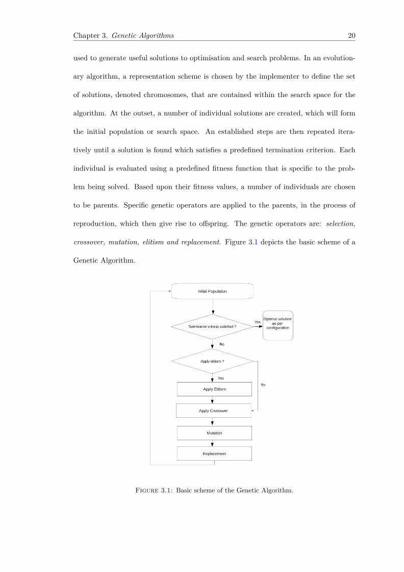
used to generate useful solutions to optimisation and search problems. In an evolution-
ary algorithm, a representation scheme is chosen by the implementer to define the set
of solutions, denoted chromosomes, that are contained within the search space for the
algorithm. At the outset, a number of individual solutions are created, which will form
the initial population or search space. An established steps are then repeated itera-
tively until a solution is found which satisfies a predefined termination criterion. Each
individual is evaluated using a predefined fitness function that is specific to the prob-
lem being solved. Based upon their fitness values, a number of individuals are chosen
to be parents. Specific genetic operators are applied to the parents, in the process of
reproduction, which then give rise to offspring. The genetic operators are: selection,
crossover, mutation, elitism and replacement. Figure 3.1 depicts the basic scheme of a
Genetic Algorithm.
Figure 3.1: Basic scheme of the Genetic Algorithm.
Chapter 3. Genetic Algorithms 21
3.1.1 Genetic Operators
3.1.1.1 Selection
The selection is the process of selecting two viable individuals, the parents, for crossover.
The purpose of selection is to isolate the fitter individuals in the population and allow
them to breed so that they can give rise to new offspring which exhibit higher fitness
values. It randomly picks chromosomes out of the population according to their fitness
function. There are two types of methodologies when it comes to selection schemes:
proportionate selection and ordinal-based selection. Proportionate-based selection picks
out individuals based upon their fitness values relative to the fitness of the other individ-
uals in the population. Ordinal-based selection schemes selects individuals upon their
rank within the population. Selection has to be maintained in balance with varying
crossover and mutation. Too strong selection means highly fit individuals will take over
the population, reducing the diversity and converging towards a solution too quickly,
which might not be optimal as it might compromise the effort of sampling a diverse
search space of candidate solutions; too weak a selection will impede and slow down
the process of evolution. The convergence rate of GA is largely determined by selection
pressure. Selection pressure gives fitter individuals a higher probability of partaking
in the mating process in order to create the next generation so that the GA can focus
on promising regions in the search space. Higher selection pressures result in higher
convergence rates and lower selection pressures lead to longer search times, though a
selection pressure that is too high will lead to convergence towards a local minimum and
not the optimal solution to the problem at hand. One needs to find a balance in order
to tune the selection process in such a way that on the one hand premature convergence
Chapter 3. Genetic Algorithms 22
is avoided but on the other hand the search time for traversal of the search does not
spiral out of control[6].
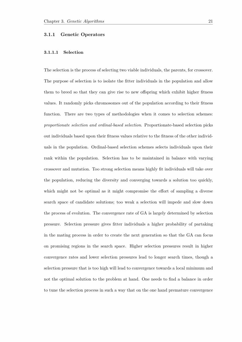
Roulette Wheel Selection In Roulette Wheel Selection an analogy can be drawn
between the whole population forming a roulette wheel with the size of of an individual’s
slot proportional to it’s fitness. Then a random selection is made analogues to ’spinning’
the wheel and throwing a figurative ’ball’ in. The probability of the ’ball’ coming to rest
in any particular slot is proportional to the arc of the slot and thus to the fitness of the
respective individual. The probability of the selection of an individual can be computed
as follows:
pi = fi∑Nj=1 fj
(3.1)
where fi is the fitness of the ith individual and N is the number of individuals. The
following depicts the approach visually:
Figure 3.2: Roulette Wheel Selection
Rank Selection Rank Selection ranks the population by the value of their fitness
value. The worst has fitness 1 and the best has fitness N. Potential parents are selected
Chapter 3. Genetic Algorithms 23
and a tournament is held to decide which of the individuals will be the parent. There
are many ways this can be accomplished. Two possible suggestions are:
1. Select a pair of individuals at random. Generate a random number, R, between 0
and 1. If R<r use the first individual as a parent. If the R≥r then use the second
individual as the parent. This is repeated to select the second parent. The value
of r is a parameter to this method.
2. Select two individuals at random. The individual with the highest evaluation
becomes the parent. Repeat to find a second parent.
This approach stifles the rate of convergence in slow but keeps up selection pressure
when the fitness variance is low, thus preserving diversity and hence leading to a better
exploitation of the search space. In effect, potential parents are selected and a random
approach is followed to decide which of the individuals will be the parent[6].
Tournament Selection Tournament selection involves running several tournaments
among a variable size of Nu individuals chosen at random from the population. The
criteria for winning the tournament is having the highest fitness value. The winner is
then injected into the mating pool for generating new offspring. The variable tournament
size and difference in fitness value of the individuals allows for selection pressure tuning,
as a bigger pool will disadvantage weaker individuals, as their chances at selection will
be smaller[6].
Random Selection This technique randomly picks a parent from the population.
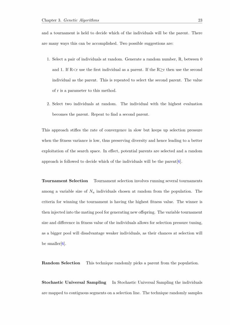
Stochastic Universal Sampling In Stochastic Universal Sampling the individuals
are mapped to contiguous segments on a selection line. The technique randomly samples
Chapter 3. Genetic Algorithms 24
all the solutions by choosing them at uniformly spaced intervals, thus exhibiting zero bias
to the selection approach and improves the chances of selection for weaker individuals[6].
The following depicts the approach visually:
Figure 3.3: Stochastic Universal Sampling Approach
3.1.1.2 Crossover
Sivanandam and Deepa[6] state that crossover is the process of mating, involving two
individuals, with the expectation that they can produce a fitter individual. The crossover
genetic operation involves the selection of a random loci to mark a cross site within the
two parent chromosomes and copy the genes to the offspring, thus giving rise to the
child that contains both parent’s genetic information and thus a new potential candidate
solution that can be interrogated for a fitness value.
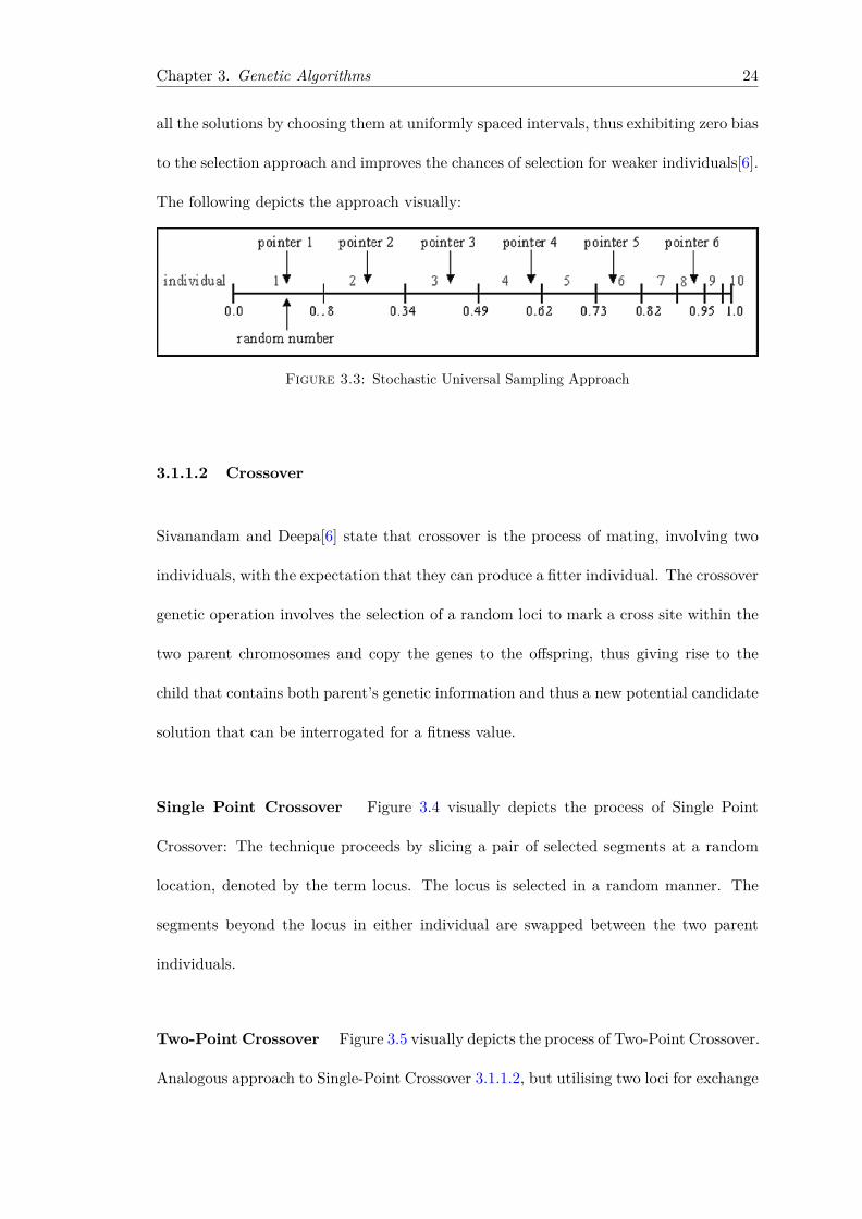
Single Point Crossover Figure 3.4 visually depicts the process of Single Point
Crossover: The technique proceeds by slicing a pair of selected segments at a random
location, denoted by the term locus. The locus is selected in a random manner. The
segments beyond the locus in either individual are swapped between the two parent
individuals.
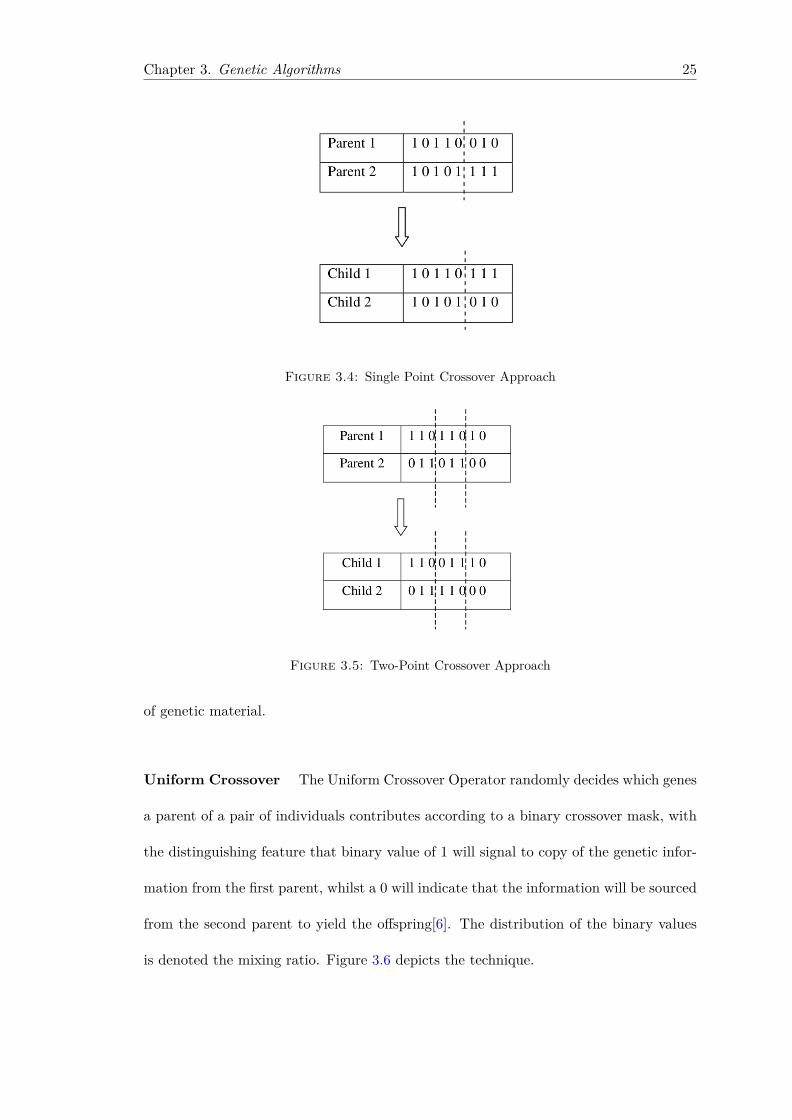
Two-Point Crossover Figure 3.5 visually depicts the process of Two-Point Crossover.
Analogous approach to Single-Point Crossover 3.1.1.2, but utilising two loci for exchange
Chapter 3. Genetic Algorithms 25
Figure 3.4: Single Point Crossover Approach
Figure 3.5: Two-Point Crossover Approach
of genetic material.
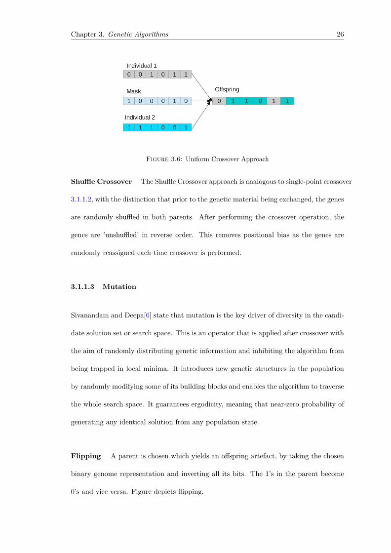
Uniform Crossover The Uniform Crossover Operator randomly decides which genes
a parent of a pair of individuals contributes according to a binary crossover mask, with
the distinguishing feature that binary value of 1 will signal to copy of the genetic infor-
mation from the first parent, whilst a 0 will indicate that the information will be sourced
from the second parent to yield the offspring[6]. The distribution of the binary values
is denoted the mixing ratio. Figure 3.6 depicts the technique.
Chapter 3. Genetic Algorithms 26
Figure 3.6: Uniform Crossover Approach
Shuffle Crossover The Shuffle Crossover approach is analogous to single-point crossover
3.1.1.2, with the distinction that prior to the genetic material being exchanged, the genes
are randomly shuffled in both parents. After performing the crossover operation, the
genes are ’unshuffled’ in reverse order. This removes positional bias as the genes are
randomly reassigned each time crossover is performed.
3.1.1.3 Mutation
Sivanandam and Deepa[6] state that mutation is the key driver of diversity in the candi-
date solution set or search space. This is an operator that is applied after crossover with
the aim of randomly distributing genetic information and inhibiting the algorithm from
being trapped in local minima. It introduces new genetic structures in the population
by randomly modifying some of its building blocks and enables the algorithm to traverse
the whole search space. It guarantees ergodicity, meaning that near-zero probability of
generating any identical solution from any population state.
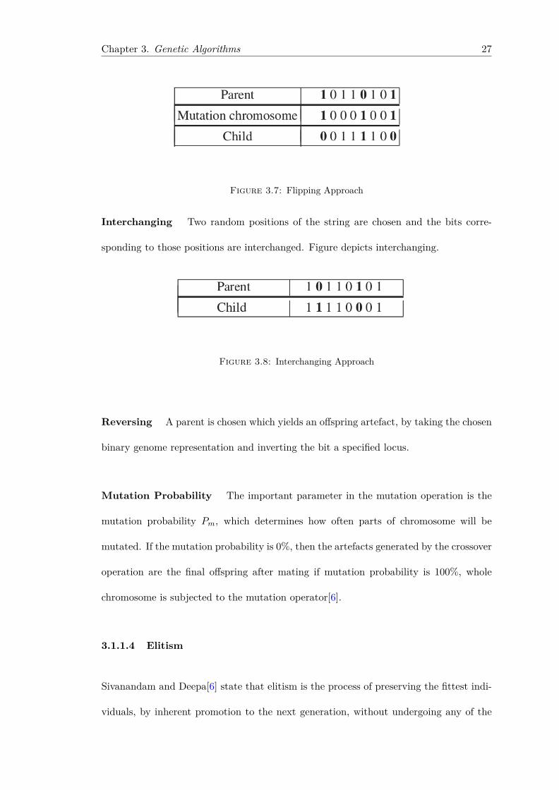
Flipping A parent is chosen which yields an offspring artefact, by taking the chosen
binary genome representation and inverting all its bits. The 1’s in the parent become
0’s and vice versa. Figure depicts flipping.
Chapter 3. Genetic Algorithms 27
Figure 3.7: Flipping Approach
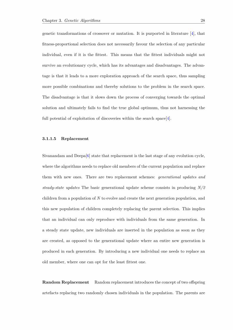
Interchanging Two random positions of the string are chosen and the bits corre-
sponding to those positions are interchanged. Figure depicts interchanging.
Figure 3.8: Interchanging Approach
Reversing A parent is chosen which yields an offspring artefact, by taking the chosen
binary genome representation and inverting the bit a specified locus.
Mutation Probability The important parameter in the mutation operation is the
mutation probability Pm, which determines how often parts of chromosome will be
mutated. If the mutation probability is 0%, then the artefacts generated by the crossover
operation are the final offspring after mating if mutation probability is 100%, whole
chromosome is subjected to the mutation operator[6].
3.1.1.4 Elitism
Sivanandam and Deepa[6] state that elitism is the process of preserving the fittest indi-
viduals, by inherent promotion to the next generation, without undergoing any of the
Chapter 3. Genetic Algorithms 28
genetic transformations of crossover or mutation. It is purported in literature [4], that
fitness-proportional selection does not necessarily favour the selection of any particular
individual, even if it is the fittest. This means that the fittest individuals might not
survive an evolutionary cycle, which has its advantages and disadvantages. The advan-
tage is that it leads to a more exploration approach of the search space, thus sampling
more possible combinations and thereby solutions to the problem in the search space.
The disadvantage is that it slows down the process of converging towards the optimal
solution and ultimately fails to find the true global optimum, thus not harnessing the
full potential of exploitation of discoveries within the search space[4].
3.1.1.5 Replacement
Sivanandam and Deepa[6] state that replacement is the last stage of any evolution cycle,
where the algorithms needs to replace old members of the current population and replace
them with new ones. There are two replacement schemes: generational updates and
steady-state updates The basic generational update scheme consists in producing N/2
children from a population of N to evolve and create the next generation population, and
this new population of children completely replacing the parent selection. This implies
that an individual can only reproduce with individuals from the same generation. In
a steady state update, new individuals are inserted in the population as soon as they
are created, as opposed to the generational update where an entire new generation is
produced in each generation. By introducing a new individual one needs to replace an
old member, where one can opt for the least fittest one.
Random Replacement Random replacement introduces the concept of two offspring
artefacts replacing two randomly chosen individuals in the population. The parents are
Chapter 3. Genetic Algorithms 29
also candidates for selection. This can be useful for continuing the search in small
populations, since weak individuals can be introduced into the population[4].
Weak Parent Replacement In Weak Parent Replacement, if two parents mate
and yield two offspring, the weaker parent will be replaced by the stronger child and
introduced in to evolved population. This introduces bias towards fitter individuals,
thus increasing the overall fitness of the population, but reducing the diversity of the
mating pool.
Both Parents Replacement In Both Parents Replacement, if two parents mate
and yield two offspring, both parents will be replaced by children and introduced in to
evolved population, thus each individual gets to breed once in the evolutionary cycle.
3.1.1.6 Advantages of Genetic Algorithms
One of the key advantages of genetic algorithms is that they are conceptually simple.
As explained in the previous section, Genetic Algorithms (GAs)can be represented by
the following steps: initialise population, evolve individuals, evaluate fitness, select indi-
viduals to survive to the next generation. Genetic Algorithms exhibit the trait of broad
applicability[6], as it can be applied to any problem whose solution domain can be quan-
tified by a function, that needs to be optimised. GAs find application in the many fields,
such as Engineering[25], Job scheduling[26], Process control, etc. They are adaptive to
changing environments, as they use the previously evolved solution to provide a basis
that one can tap into to make further improvements to the solution domain[6]. Contrary
to other optimisation methodologies, GAs do not need to return to the initial state of
computation. They can be implemented for all sorts of problem types, as long as one
Chapter 3. Genetic Algorithms 30
adheres to the basic guidelines. The evolution process lends itself to parallel process-
ing techniques[21], which opens up new avenues to explore in terms of hybridisation
with other optimisation techniques, which can give rise to more efficient ways to solve
problems in general. One could for example use a conjugate-gradient minimisation after
instituting a primary search with Genetic Algorithms[6].
3.1.2 Non-binary Encodings
By convention, a chromosome is a sequence of symbols and that these symbols are binary
in form, thus exhibiting a cardinality of 2. The most effective approach is though when
the encoding or the alphabet employed is problem-specific and most fittingly represents
the solutions in the search space, as it will be illustrated in this thesis. It shows that
higher-cardinality alphabets are more suited to certain type of problems[5, 6]. Empirical
studies of high-cardinality alphabets have typically applied chromosomes where each
encoding represents an integer[22, 27], or a floating-point number[28]. But those present
problems, in terms of the subject matter covered, on how to apply genetic operators
such as mutation and crossover to those encodings.[5] defines the following Crossover
and Mutation genetic operators for non-binary representations:
1. Crossover:
• Average : Apply the arithmetic average of the two parent genes.
• Geometric mean: Apply the square root of the product of the two values.
• Extension: Take the difference between two values and add to the higher or
subtract it from the lower of the two values
2. Mutation:
Chapter 3. Genetic Algorithms 31
• Random replacement : Replace the value at specific locus with a random
value
• Creep : Add and subtract a small, randomly generated amount.
• Geometric creep: Multiply by random amount close to one.
The random number generator in the above operations might base on a variety of dis-
tributions from exponential, uniform within a range to Gaussian or binomial models,
Gaussian being the preferred one.[6] states that experiments were conducted with float-
ing point representations and it was determined that floating point representations are
faster, more consistent from run to run, and provide higher precision, especially in large
domains where binary coding would require unusually long representations. At the same
time its performance can be enhanced by the application of special operators to achieve
high performance accuracy[28].
3.1.3 Knowledge Based Techniques
GA schemes usually apply the traditional crossover and mutation operators, but in
certain cases and also in this research undertaken in this thesis, I would rather advocate
using a specific type of operators for the task at hand, preferentially that is guided using
domain knowledge. This makes the GA less generic and more problem specific, but may
improve performance significantly[6, 29]. Where a GA is being designed to tackle a real-
world problem, and has to compete with other search and optimization techniques, the
incorporation of domain knowledge often is advisable[6, 29]. Domain knowledge may be
used to prevent obviously unfit chromosomes or prevent the algorithm from honing in
on a sub-optimal solution, or even violate problem constraints, from being produced in
the first place[6, 29]. This avoids wasting time evaluating such individuals, and avoids
Chapter 3. Genetic Algorithms 32
introducing poor performers into the population. [6] states that areas of utilisation
would be:
• Guiding the initialisation of the population at the beginning of the process[6].
• Guiding the crossover operator, so that the crossover operation does in fact yield
fitter offspring in order to prevent weaker individuals being introduced into suc-
cessive matings pools[6].
• Guiding the mutation operator. For example, the application of gradient like
bitwise (G-bit) improvement for one or more highly fit chromosomes, allows the
change of each bit one at a time to see if the fitness improves. If it does, one would
replace the original with the altered chromosome[6].
[6] advise to utilise hybrid GA schemes, combining GAs with other heuristic search
algorithms, such as hill climbing or greedy search. The GA would be utilised to locate
the solution in the search space or come close to it and then use those optimisation
schemes to hone in on the optimal value, thus improving the efficiency and competence
of the GA[6].
3.2 Parallel Genetic Algorithms
3.2.1 Discretised Genetic Algorithms
Genetic Algorithms are very effective in solving very complex problems. This positive
trait can be unfortunately offset by very long execution times, due to the traversal of the
search space. As mentioned in section 3.1.1.6, GAs lend themselves to parallelisation
and thus the fitness values can be determined independently for each of the candidate
Chapter 3. Genetic Algorithms 33
solutions, utilising one of the parallelisation schemes: master-slave models, multiple-
deme, and fine-grained PGAs[6]. I will focus on the master-slave models and the multiple-
deme parallelisation schemes. The master-slave parallelisation scheme are relatively easy
to implement. On the other hand, the multiple-deme parallelisation scheme currently
dominates the research on PGAs due its complexty and the fact that its behavior is
affected by many parameters[6].
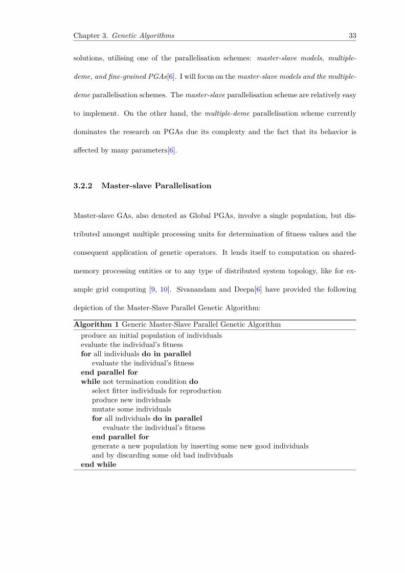
3.2.2 Master-slave Parallelisation
Master-slave GAs, also denoted as Global PGAs, involve a single population, but dis-
tributed amongst multiple processing units for determination of fitness values and the
consequent application of genetic operators. It lends itself to computation on shared-
memory processing entities or to any type of distributed system topology, like for ex-
ample grid computing [9, 10]. Sivanandam and Deepa[6] have provided the following
depiction of the Master-Slave Parallel Genetic Algorithm:
Algorithm 1 Generic Master-Slave Parallel Genetic Algorithmproduce an initial population of individualsevaluate the individual’s fitnessfor all individuals do in parallel
evaluate the individual’s fitnessend parallel forwhile not termination condition do
select fitter individuals for reproductionproduce new individualsmutate some individualsfor all individuals do in parallel
evaluate the individual’s fitnessend parallel forgenerate a new population by inserting some new good individualsand by discarding some old bad individuals
end while
Chapter 3. Genetic Algorithms 34
Master-slave PGAs are easy to implement and they can be a very efficient method of
parallelisation when the evaluation needs considerable computations, thus reducing the
execution time of the algorithm. Besides, the method has the advantage of not altering
the search behaviour of the GA[6, 30], so all the theory available for simple GAs can be
applied directly without any modifications[6].
3.2.3 Multiple-deme Parallelisation
Multiple-population or Multiple-deme PGAs allow for the populations to be partitioned
into disjoint, autonomous sub-populations and undergo subsequent evolution, indepen-
dently of each other, thus in parallel. The complexity arises when trying to find a balance
between the communication cost, trying to constrain it to a minimum, whilst ensuring a
diverse mixture of individuals from the respective sub search spaces. I need to establish
an optimal segment sizing approach, in order to find the optimal number of demes which
will ensure diversity and a comprehensive set of candidate solutions. This will lead to
optimal convergence[10]. Multiple-deme parallel GAs are also called ”coarse-grained” or
”distributed” GAs, due to the fact that the communication to computation ratio is low,
and they are often implemented on distributed-memory computers[30]. They consist
of several sub-populations that undergo evolution independently of each other and at
pre-defined intervals, called epochs, exchange individuals with other sub-populations.
The arrangement and interconnectivity between the different sub-populations resembles
an archipelago, a cluster of islands, thus deeming the Multiple-deme model an ”island
model”. These algorithms are quite popular, but very difficult to understand, configure
and optimise due to unpredictability of the migration process. Additionally, there exist
many parameters that need to be configured that affect their accuracy and efficiency [31].
Chapter 3. Genetic Algorithms 35
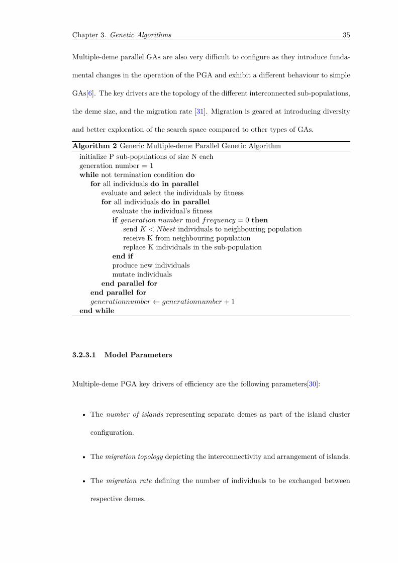
Multiple-deme parallel GAs are also very difficult to configure as they introduce funda-
mental changes in the operation of the PGA and exhibit a different behaviour to simple
GAs[6]. The key drivers are the topology of the different interconnected sub-populations,
the deme size, and the migration rate [31]. Migration is geared at introducing diversity
and better exploration of the search space compared to other types of GAs.
Algorithm 2 Generic Multiple-deme Parallel Genetic Algorithminitialize P sub-populations of size N eachgeneration number = 1while not termination condition do
for all individuals do in parallelevaluate and select the individuals by fitnessfor all individuals do in parallel
evaluate the individual’s fitnessif generation number mod frequency = 0 then
send K < Nbest individuals to neighbouring populationreceive K from neighbouring populationreplace K individuals in the sub-population
end ifproduce new individualsmutate individuals
end parallel forend parallel forgenerationnumber ← generationnumber + 1
end while
3.2.3.1 Model Parameters
Multiple-deme PGA key drivers of efficiency are the following parameters[30]:
• The number of islands representing separate demes as part of the island cluster
configuration.
• The migration topology depicting the interconnectivity and arrangement of islands.
• The migration rate defining the number of individuals to be exchanged between
respective demes.
Chapter 3. Genetic Algorithms 36
• The migration frequency defining how often a exchange of individuals transpires.
This measure is directly related to the epoch, as the it signifies the period at which
the migrations take place.
• The migration algorithm specifying all the remaining details.
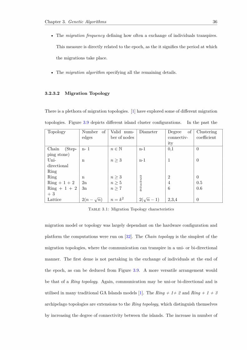
3.2.3.2 Migration Topology
There is a plethora of migration topologies. [1] have explored some of different migration
topologies. Figure 3.9 depicts different island cluster configurations. In the past the
Topology Number ofedges
Valid num-ber of nodes
Diameter Degree ofconnectiv-ity
Clusteringcoefficient
Chain (Step-ping stone)
n- 1 n ∈ N n-1 0,1 0
Uni-directionalRing
n n ≥ 3 n-1 1 0
Ring n n ≥ 3 n2 2 0
Ring + 1 + 2 2n n ≥ 5 n4 4 0.5
Ring + 1 + 2+ 3
3n n ≥ 7 n6 6 0.6
Lattice 2(n−√n) n = k2 2(
√n− 1) 2,3,4 0
Table 3.1: Migration Topology characteristics
migration model or topology was largely dependant on the hardware configuration and
platform the computations were run on [32]. The Chain topology is the simplest of the
migration topologies, where the communication can transpire in a uni- or bi-directional
manner. The first deme is not partaking in the exchange of individuals at the end of
the epoch, as can be deduced from Figure 3.9. A more versatile arrangement would
be that of a Ring topology. Again, communication may be uni-or bi-directional and is
utilised in many traditional GA Islands models [1]. The Ring + 1+ 2 and Ring + 1 + 3
archipelago topologies are extensions to the Ring topology, which distinguish themselves
by increasing the degree of connectivity between the islands. The increase in number of
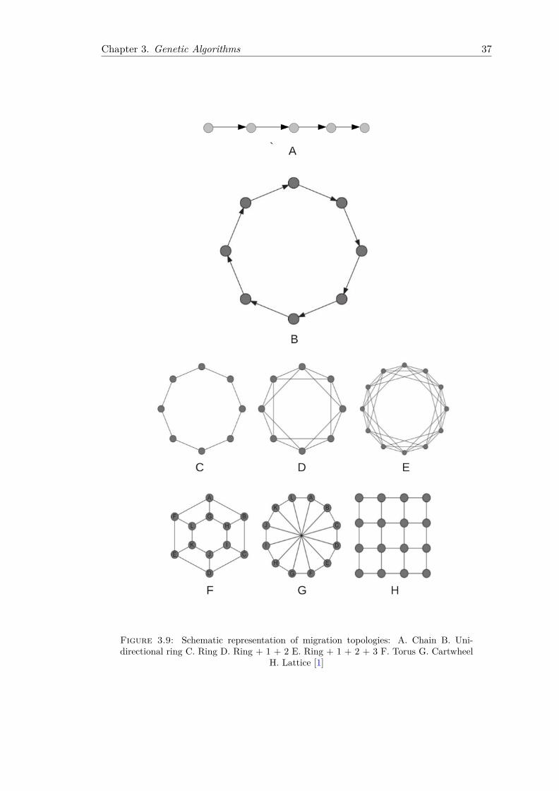
Chapter 3. Genetic Algorithms 37
Figure 3.9: Schematic representation of migration topologies: A. Chain B. Uni-directional ring C. Ring D. Ring + 1 + 2 E. Ring + 1 + 2 + 3 F. Torus G. Cartwheel
H. Lattice [1]
Chapter 3. Genetic Algorithms 38
edges is tabulated in 3.1. The topologies also affect the number of nodes that comprise
the topology arrangement, which entail a minimum number of nodes to be configured,
in order to be able to harness the full potential of the specific migration approach.
3.2.3.3 Number of Islands
The number of islands is dependant on the computing platform used , the underlying
hardware configuration or the migration topology utilised. PGAs scale very well and
with more hardware at my disposal for the goal of computation, I am able to partition the
search space into more sub-populations and henceforth improve the overall efficiency of
the computations. The migration topology also has a pronounced effect on the number
of sub-populations utilised. As tabulated in Section 3.2.3.2, the topology chosen will
necessitate a certain number of islands to be declared. In using a specific migration
scheme, I need to be cognisant of the fact that the greater the number of edges, the
greater the number of exchanges between the respective sub-populations within the
archipelago and also the higher the communication overhead. But [32] state, that the
higher the number of islands, the better the result of the computation. They also state
that this only holds for certain type of problems and algorithms, so quintessentially
there is no rule of thumb as to the optimal number of islands. The onus lies with
the researcher to apply different migration topologies and investigate the effects of the
different parameters on the efficiency of the algorithm.
Chapter 4
Computational Platform
In order to be able to fully harness the capabilities of a Parallel Genetic Algorithm as
described in the Chapter 3, I need to make use of a parallel computing platform. CUDA
is such a platform. It is a platform and a programming model invented by NVIDIA. This
chapter will firstly introduce conventional parallel computing architectures and then
acquaint the reader with the CUDA parallel computing platform, specifically chosen
for the task of delivering cluster analysis results in an efficient manner. It forms the
backbone of the research undertaken and also allows for the proposed clustering analysis
approach to be employed.
4.1 Parallel computing
4.1.1 Architectures
There exist several different parallel architectures. They can be grouped into four cat-
egories based upon the number of instructions that can be performed concurrently and
the number of data streams these instructions can operate upon. The classifications were
39
Chapter 4. Computational Platform 40
first proposed by Flynn[33] in 1966 and are the following: single instruction stream/s-
ingle data stream (SISD), single instruction stream/multiple data stream (SIMD), mul-
tiple instruction stream/single data stream (MISD), and multiple data stream/multiple
instruction stream (MIMD)[34]. The MIMD classification has replaced the SIMD as
the de facto parallel platform today. The MIMD classification includes shared memory
multiprocessor systems and message-passing multi-computers[35]. The architecture of
shared memory multiprocessors focuses on the idea of a globally addressable memory
location. In shared memory multiprocessor machines, also referred to as symmetric mul-
tiprocessors (SMPs), the memory location is physically equidistant or appears physically
equidistant from all processors. Variations on the traditional shared memory architec-
ture exist that relax the scalability limitations of traditional shared memory machines,
yet still provide the appearance of equidistant memory. These architectures are re-
ferred to as distributed shared memory machines and fall under the shared memory
category. These include cache coherent non-uniform access (CC-NUMA) machines[34].
In message passing multi-computers, or distributed memory architectures, each proces-
sor has its own memory location and the memory is not globally addressable. Parallel
architectures in the distributed memory classification do not suffer from the scalability
restrictions of the shared memory architectures and hence have gained popularity in the
high performance computing segment.
4.1.2 Parallel programming and design paradigms
Programming in parallel environments has being reliant on the use of compiler directives
and libraries. Those allow for the integration of parallelism directly into existing code
instead of having to use a new language, that is designed specifically for the parallel
Chapter 4. Computational Platform 41
environment. This allows the programmer to stay at least somewhat in a familiar en-
vironment, where syntax is concerned and allows already written and tested code to be
in some cases fairly easily parallelised. Programming in the distributed memory envi-
ronment has been dominated by message passing interface (MPI) for the last several
years. MPI provides a standard for implementations of message passing libraries for
many parallel architectures; it is highly portable and can also be used in shared memory
environments[36]. Shared memory programming has seen a resurgence of interest with
the development of OpenMP, which utilizes compiler directives to easily parallelise sec-
tions of code[37]. The following design paradigms are key to programming in a parallel
environment and determine the success or failure of an implementation:data placement,
communication latency and synchronisation[38].
4.1.3 Rationale
A proper design of a parallel algorithms along with careful consideration of the chosen
platform leads to substantial reductions in execution time. Additionally, new algorithm
designs provide benefits in solution quality due to the application of parallelism. How-
ever, without careful consideration to design and platform choice, it is also possible to
not obtain the full benefit of the parallel computing environment and in the worst case
negative results in performance[39].
4.2 GPU
Graphics processor units (GPU), traditionally designed for graphics rendering have
emerged as massively-parallel ’co-processors’ to the central processing unit(CPU). Ac-
cording to Flynn’s taxonomy, as stated in 4.1.1, GPUs are classified as SIMDs and belong
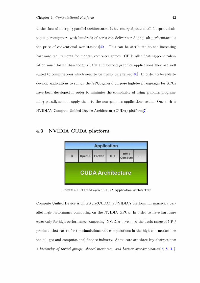
Chapter 4. Computational Platform 42
to the class of emerging parallel architectures. It has emerged, that small-footprint desk-
top supercomputers with hundreds of cores can deliver teraflops peak performance at
the price of conventional workstations[40]. This can be attributed to the increasing
hardware requirements for modern computer games. GPUs offer floating-point calcu-
lation much faster than today’s CPU and beyond graphics applications they are well
suited to computations which need to be highly parallelised[40]. In order to be able to
develop applications to run on the GPU, general purpose high-level languages for GPUs
have been developed in order to minimise the complexity of using graphics program-
ming paradigms and apply them to the non-graphics applications realm. One such is
NVIDIA’s Compute Unified Device Architecture(CUDA) platform[7].
4.3 NVIDIA CUDA platform
Figure 4.1: Three-Layered CUDA Application Architecture
Compute Unified Device Architecture(CUDA) is NVIDIA’s platform for massively par-
allel high-performance computing on the NVIDIA GPUs. In order to have hardware
cater only for high performance computing, NVIDIA developed the Tesla range of GPU
products that caters for the simulations and computations in the high-end market like
the oil, gas and computational finance industry. At its core are three key abstractions:
a hierarchy of thread groups, shared memories, and barrier synchronisation[7, 8, 41].
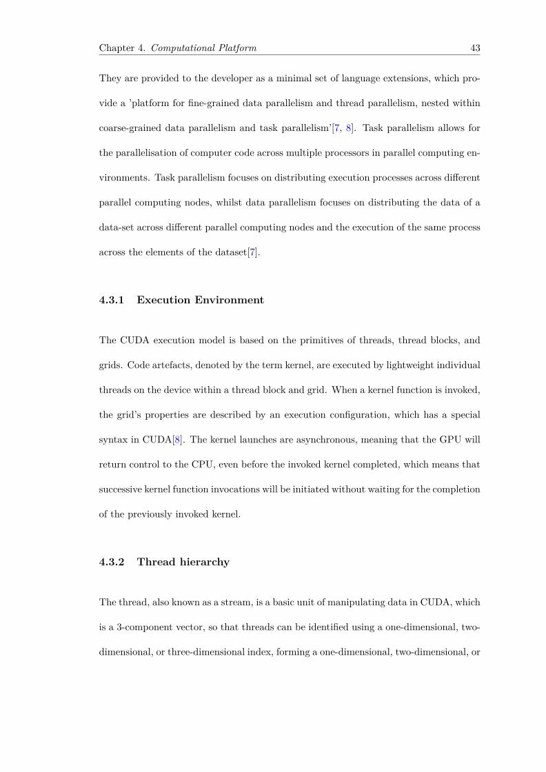
Chapter 4. Computational Platform 43
They are provided to the developer as a minimal set of language extensions, which pro-
vide a ’platform for fine-grained data parallelism and thread parallelism, nested within
coarse-grained data parallelism and task parallelism’[7, 8]. Task parallelism allows for
the parallelisation of computer code across multiple processors in parallel computing en-
vironments. Task parallelism focuses on distributing execution processes across different
parallel computing nodes, whilst data parallelism focuses on distributing the data of a
data-set across different parallel computing nodes and the execution of the same process
across the elements of the dataset[7].
4.3.1 Execution Environment
The CUDA execution model is based on the primitives of threads, thread blocks, and
grids. Code artefacts, denoted by the term kernel, are executed by lightweight individual
threads on the device within a thread block and grid. When a kernel function is invoked,
the grid’s properties are described by an execution configuration, which has a special
syntax in CUDA[8]. The kernel launches are asynchronous, meaning that the GPU will
return control to the CPU, even before the invoked kernel completed, which means that
successive kernel function invocations will be initiated without waiting for the completion
of the previously invoked kernel.
4.3.2 Thread hierarchy
The thread, also known as a stream, is a basic unit of manipulating data in CUDA, which
is a 3-component vector, so that threads can be identified using a one-dimensional, two-
dimensional, or three-dimensional index, forming a one-dimensional, two-dimensional, or
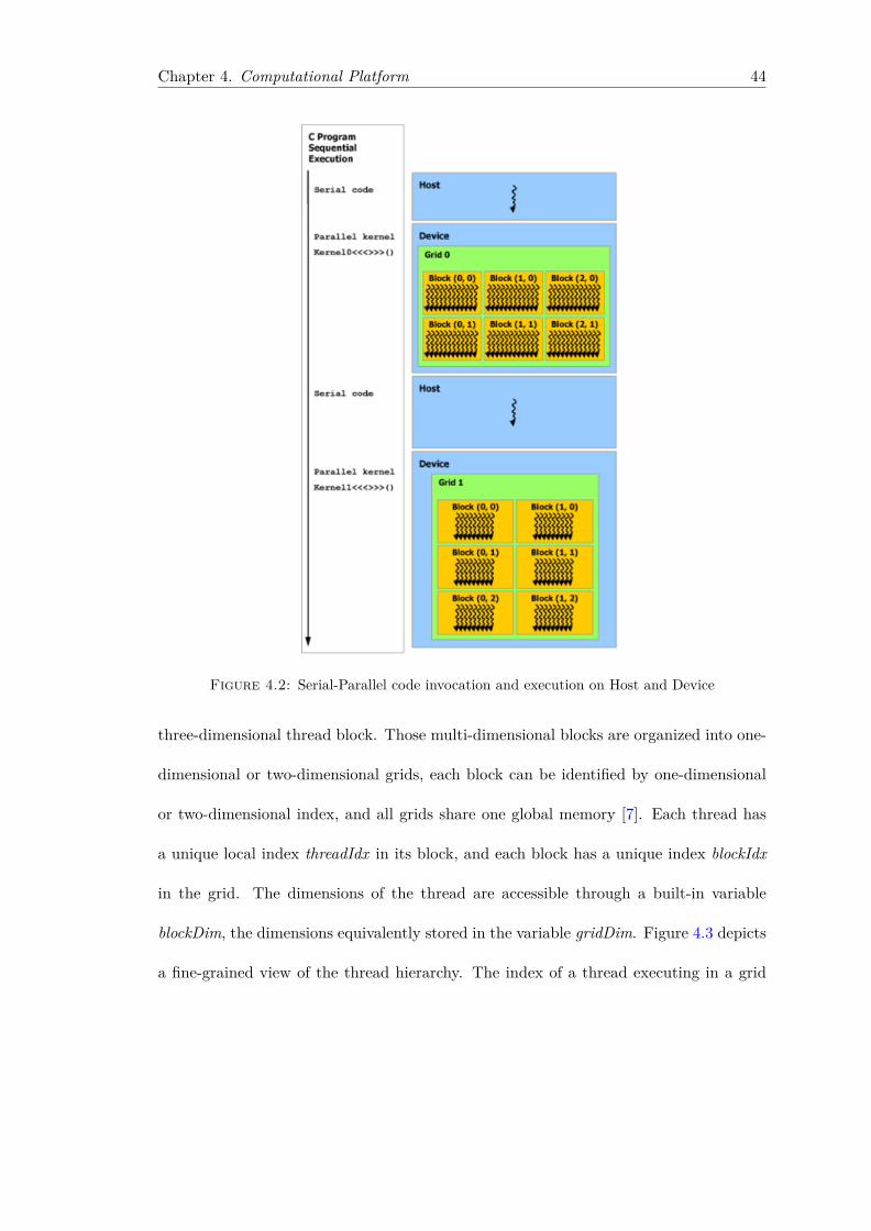
Chapter 4. Computational Platform 44
Figure 4.2: Serial-Parallel code invocation and execution on Host and Device
three-dimensional thread block. Those multi-dimensional blocks are organized into one-
dimensional or two-dimensional grids, each block can be identified by one-dimensional
or two-dimensional index, and all grids share one global memory [7]. Each thread has
a unique local index threadIdx in its block, and each block has a unique index blockIdx
in the grid. The dimensions of the thread are accessible through a built-in variable
blockDim, the dimensions equivalently stored in the variable gridDim. Figure 4.3 depicts
a fine-grained view of the thread hierarchy. The index of a thread executing in a grid
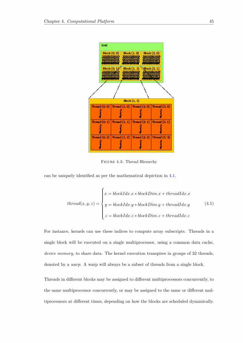
Chapter 4. Computational Platform 45
Figure 4.3: Thread Hierarchy
can be uniquely identified as per the mathematical depiction in 4.1.
thread(x, y, z) =
x = blockIdx.x ∗ blockDim.x+ threadIdx.x
y = blockIdx.y ∗ blockDim.y + threadIdx.y
z = blockIdx.z ∗ blockDim.z + threadIdx.z
(4.1)
For instance, kernels can use these indices to compute array subscripts. Threads in a
single block will be executed on a single multiprocessor, using a common data cache,
device memory, to share data. The kernel execution transpires in groups of 32 threads,
denoted by a warp. A warp will always be a subset of threads from a single block.
Threads in different blocks may be assigned to different multiprocessors concurrently, to
the same multiprocessor concurrently, or may be assigned to the same or different mul-
tiprocessors at different times, depending on how the blocks are scheduled dynamically.
Chapter 4. Computational Platform 46
There is a hard limit on the size of a thread block, this being 512 threads or 16 warps
for Tesla, 1024 threads or 32 warps for Fermi. Thread blocks are always created in warp
units, so there is no point in trying to create a thread block of size that is not a multiple
of 32 threads; all thread blocks in the whole grid will have the same size and shape. A
Tesla multiprocessor can have 1024 threads simultaneously active, or 32 warps. These
can come from 2 thread blocks of 16 warps, or 3 thread blocks of 10 warps, 4 thread
blocks of 8 warps, and so on up to 8 blocks of 4 warps; there is another hard limit of
8 thread blocks simultaneously active on a single multiprocessor. As mentioned, Fermi
can have 48 simultaneously active warps, equivalent to 1536 threads, from up to 8 thread
blocks.
4.3.3 Memory hierarchy
There are multiple data caches that CUDA threads may access data from during their
execution, as illustrated by Figure 4.4 [7].
4.3.3.1 Registers
Registers are the fastest memory units on a GPU, and each multiprocessor on the GPU
has a large, but limited, register file which is divided amongst threads residing on that
multiprocessor. Registers are private for each thread, and if the threads use more reg-
isters than at it’s disposal, a register spillover incurs, with L1 cache and global memory
being affected. The more threads utilised, the lower the register availability to each
thread [42].
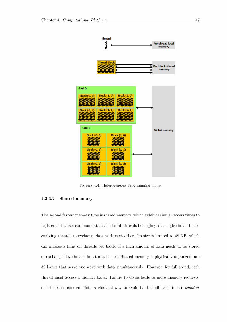
Chapter 4. Computational Platform 47
Figure 4.4: Heterogeneous Programming model
4.3.3.2 Shared memory
The second fastest memory type is shared memory, which exhibits similar access times to
registers. It acts a common data cache for all threads belonging to a single thread block,
enabling threads to exchange data with each other. Its size is limited to 48 KB, which
can impose a limit on threads per block, if a high amount of data needs to be stored
or exchanged by threads in a thread block. Shared memory is physically organized into
32 banks that serve one warp with data simultaneously. However, for full speed, each
thread must access a distinct bank. Failure to do so leads to more memory requests,
one for each bank conflict. A classical way to avoid bank conflicts is to use padding,
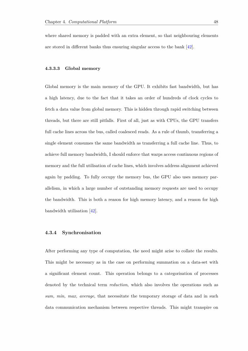
Chapter 4. Computational Platform 48
where shared memory is padded with an extra element, so that neighbouring elements
are stored in different banks thus ensuring singular access to the bank [42].
4.3.3.3 Global memory
Global memory is the main memory of the GPU. It exhibits fast bandwidth, but has
a high latency, due to the fact that it takes an order of hundreds of clock cycles to
fetch a data value from global memory. This is hidden through rapid switching between
threads, but there are still pitfalls. First of all, just as with CPUs, the GPU transfers
full cache lines across the bus, called coalesced reads. As a rule of thumb, transferring a
single element consumes the same bandwidth as transferring a full cache line. Thus, to
achieve full memory bandwidth, I should enforce that warps access continuous regions of
memory and the full utilisation of cache lines, which involves address alignment achieved
again by padding. To fully occupy the memory bus, the GPU also uses memory par-
allelism, in which a large number of outstanding memory requests are used to occupy
the bandwidth. This is both a reason for high memory latency, and a reason for high
bandwidth utilisation [42].
4.3.4 Synchronisation
After performing any type of computation, the need might arise to collate the results.
This might be necessary as in the case on performing summation on a data-set with
a significant element count. This operation belongs to a categorisation of processes
denoted by the technical term reduction, which also involves the operations such as
sum, min, max, average, that necessitate the temporary storage of data and in such
data communication mechanism between respective threads. This might transpire on
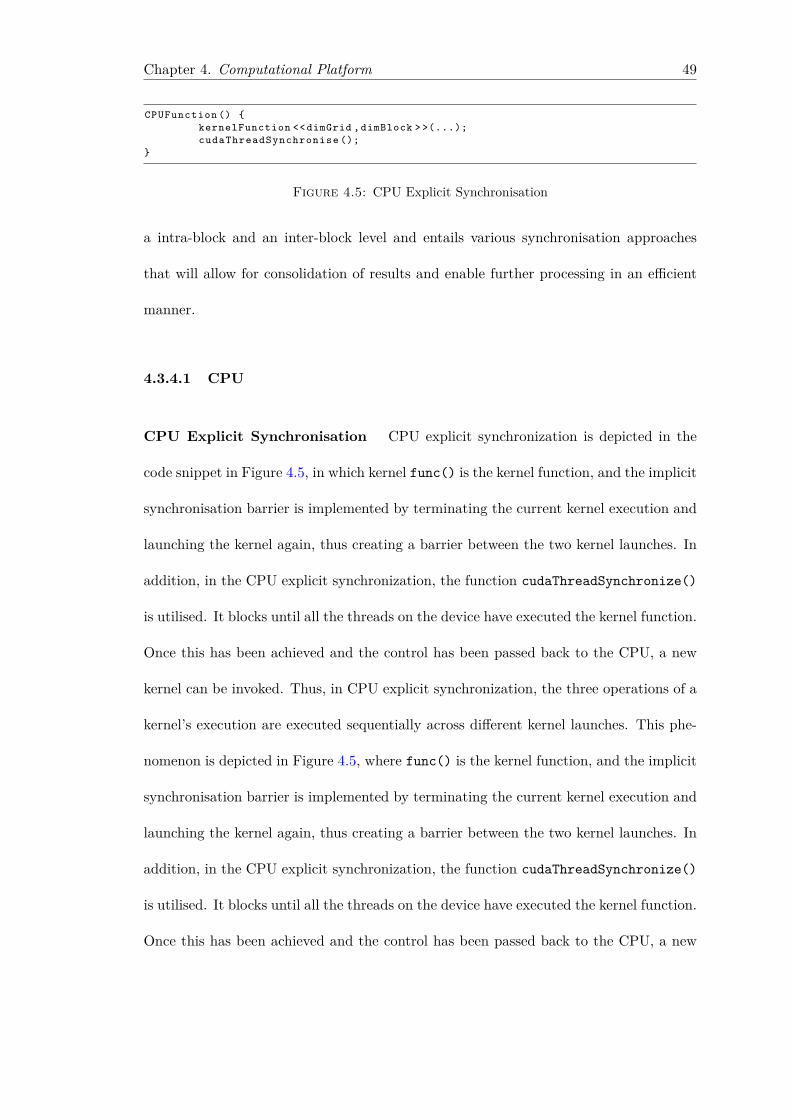
Chapter 4. Computational Platform 49
CPUFunction () {kernelFunction <<dimGrid ,dimBlock > >(...);cudaThreadSynchronise ();
}
Figure 4.5: CPU Explicit Synchronisation
a intra-block and an inter-block level and entails various synchronisation approaches
that will allow for consolidation of results and enable further processing in an efficient
manner.
4.3.4.1 CPU
CPU Explicit Synchronisation CPU explicit synchronization is depicted in the
code snippet in Figure 4.5, in which kernel func() is the kernel function, and the implicit
synchronisation barrier is implemented by terminating the current kernel execution and
launching the kernel again, thus creating a barrier between the two kernel launches. In
addition, in the CPU explicit synchronization, the function cudaThreadSynchronize()
is utilised. It blocks until all the threads on the device have executed the kernel function.
Once this has been achieved and the control has been passed back to the CPU, a new
kernel can be invoked. Thus, in CPU explicit synchronization, the three operations of a
kernel’s execution are executed sequentially across different kernel launches. This phe-
nomenon is depicted in Figure 4.5, where func() is the kernel function, and the implicit
synchronisation barrier is implemented by terminating the current kernel execution and
launching the kernel again, thus creating a barrier between the two kernel launches. In
addition, in the CPU explicit synchronization, the function cudaThreadSynchronize()
is utilised. It blocks until all the threads on the device have executed the kernel function.
Once this has been achieved and the control has been passed back to the CPU, a new
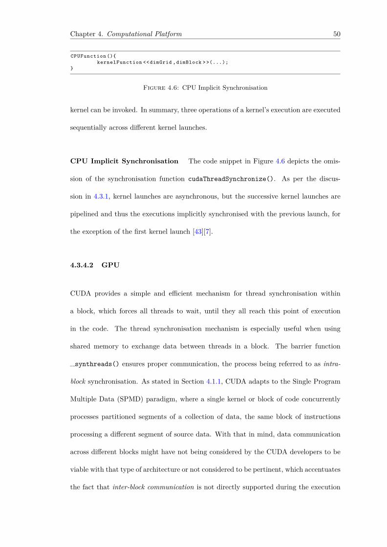
Chapter 4. Computational Platform 50
CPUFunction (){kernelFunction <<dimGrid ,dimBlock > >(...);
}
Figure 4.6: CPU Implicit Synchronisation
kernel can be invoked. In summary, three operations of a kernel’s execution are executed
sequentially across different kernel launches.
CPU Implicit Synchronisation The code snippet in Figure 4.6 depicts the omis-
sion of the synchronisation function cudaThreadSynchronize(). As per the discus-
sion in 4.3.1, kernel launches are asynchronous, but the successive kernel launches are
pipelined and thus the executions implicitly synchronised with the previous launch, for
the exception of the first kernel launch [43][7].
4.3.4.2 GPU
CUDA provides a simple and efficient mechanism for thread synchronisation within
a block, which forces all threads to wait, until they all reach this point of execution
in the code. The thread synchronisation mechanism is especially useful when using
shared memory to exchange data between threads in a block. The barrier function
synthreads() ensures proper communication, the process being referred to as intra-
block synchronisation. As stated in Section 4.1.1, CUDA adapts to the Single Program
Multiple Data (SPMD) paradigm, where a single kernel or block of code concurrently
processes partitioned segments of a collection of data, the same block of instructions
processing a different segment of source data. With that in mind, data communication
across different blocks might have not being considered by the CUDA developers to be
viable with that type of architecture or not considered to be pertinent, which accentuates
the fact that inter-block communication is not directly supported during the execution
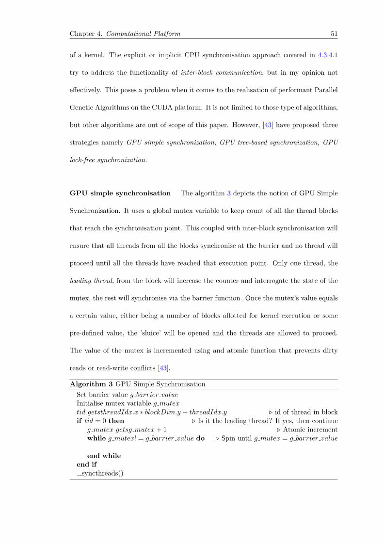
Chapter 4. Computational Platform 51
of a kernel. The explicit or implicit CPU synchronisation approach covered in 4.3.4.1
try to address the functionality of inter-block communication, but in my opinion not
effectively. This poses a problem when it comes to the realisation of performant Parallel
Genetic Algorithms on the CUDA platform. It is not limited to those type of algorithms,
but other algorithms are out of scope of this paper. However, [43] have proposed three
strategies namely GPU simple synchronization, GPU tree-based synchronization, GPU
lock-free synchronization.
GPU simple synchronisation The algorithm 3 depicts the notion of GPU Simple
Synchronisation. It uses a global mutex variable to keep count of all the thread blocks
that reach the synchronisation point. This coupled with inter-block synchronisation will
ensure that all threads from all the blocks synchronise at the barrier and no thread will
proceed until all the threads have reached that execution point. Only one thread, the
leading thread, from the block will increase the counter and interrogate the state of the
mutex, the rest will synchronise via the barrier function. Once the mutex’s value equals
a certain value, either being a number of blocks allotted for kernel execution or some
pre-defined value, the ’sluice’ will be opened and the threads are allowed to proceed.
The value of the mutex is incremented using and atomic function that prevents dirty
reads or read-write conflicts [43].
Algorithm 3 GPU Simple SynchronisationSet barrier value g barrier valueInitialise mutex variable g mutextid getsthreadIdx.x ∗ blockDim.y + threadIdx.y . id of thread in blockif tid = 0 then . Is it the leading thread? If yes, then continue
g mutex getsg mutex+ 1 . Atomic incrementwhile g mutex! = g barrier value do . Spin until g mutex = g barrier value
end whileend if
syncthreads()
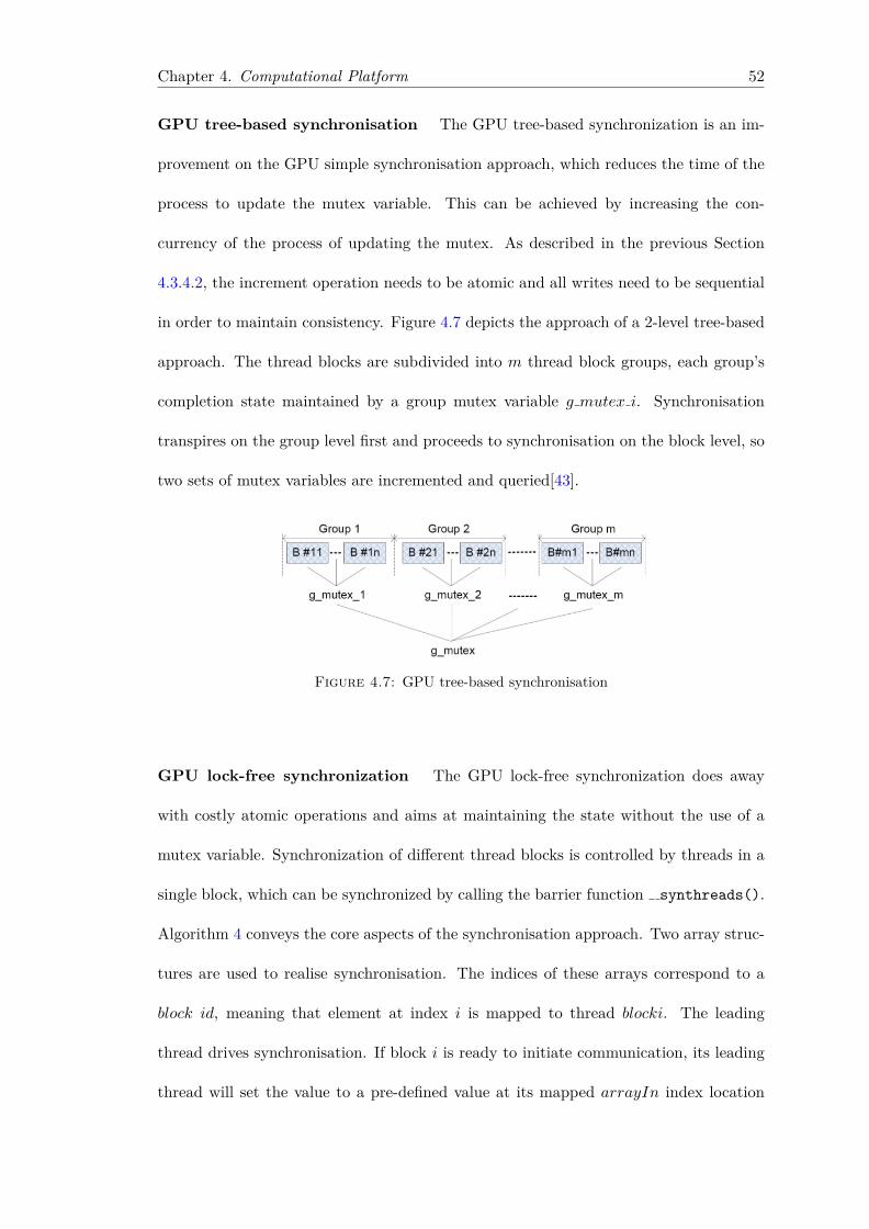
Chapter 4. Computational Platform 52
GPU tree-based synchronisation The GPU tree-based synchronization is an im-
provement on the GPU simple synchronisation approach, which reduces the time of the
process to update the mutex variable. This can be achieved by increasing the con-
currency of the process of updating the mutex. As described in the previous Section
4.3.4.2, the increment operation needs to be atomic and all writes need to be sequential
in order to maintain consistency. Figure 4.7 depicts the approach of a 2-level tree-based
approach. The thread blocks are subdivided into m thread block groups, each group’s
completion state maintained by a group mutex variable g mutex i. Synchronisation
transpires on the group level first and proceeds to synchronisation on the block level, so
two sets of mutex variables are incremented and queried[43].
Figure 4.7: GPU tree-based synchronisation
GPU lock-free synchronization The GPU lock-free synchronization does away
with costly atomic operations and aims at maintaining the state without the use of a
mutex variable. Synchronization of different thread blocks is controlled by threads in a
single block, which can be synchronized by calling the barrier function synthreads().
Algorithm 4 conveys the core aspects of the synchronisation approach. Two array struc-
tures are used to realise synchronisation. The indices of these arrays correspond to a
block id, meaning that element at index i is mapped to thread blocki. The leading
thread drives synchronisation. If block i is ready to initiate communication, its leading
thread will set the value to a pre-defined value at its mapped arrayIn index location
Chapter 4. Computational Platform 53
and will wait until the same value has been set at its mapped arrayOut index location,
before it the ’sluice’ is opened and the threads within all the blocks can proceed beyond
the synchronisation point. Analogous to having a leading thread in block, a leading
block is chosen to drive the next stage of synchronisation, namely the first block. Any
other block in the grid can be chosen, but in order to maintain consistency and clarity
I should revert to using the first block of the grid. All the threads in the leading block
will read the value in arrayIn, i.e. the ith thread will read the value at index i in the
array. Should the value be that of the pre-defined barrier value, then the thread will set
the value of the corresponding element at index position i in arrayOut. This approach
further improves the level of concurrency as all the threads of the leading block are
assigned to oversee the state of the blocks in the grid and pull the proverbial lever so
that collectively they can open the ’sluice’ [43].
Disadvantages of GPU synchronisation Due to the latency on the call between
CPU and GPU, CPU synchronisation incurs a significant overhead and GPU synchro-
nisation is preferred. There is a downside to GPU synchronisation though, that in my
mind discredits the whole investigation and methodology. A constraint exits on the
number of blocks that can be configures and the number needs to smaller or equal to
the Streaming Multiprocessors(SM) on the GPU card. If the number of thread blocks
is bigger than the number of SMs on the card, execution will deadlock. This is due to
the non-preemptive warp scheduling behaviour of the GPU. If the number is bigger, this
will then automatically infer that more than one thread block will be assigned to a SM
for execution. The unscheduled thread blocks will not be executed, due to the fact that
the active blocks, resident on the SM, are in a state of busy-waiting for the unscheduled
thread blocks at the synchronisation point. Further, the published GPU synchronisation
approaches just seem not to be a viable option for synchronisation. I am constrained to
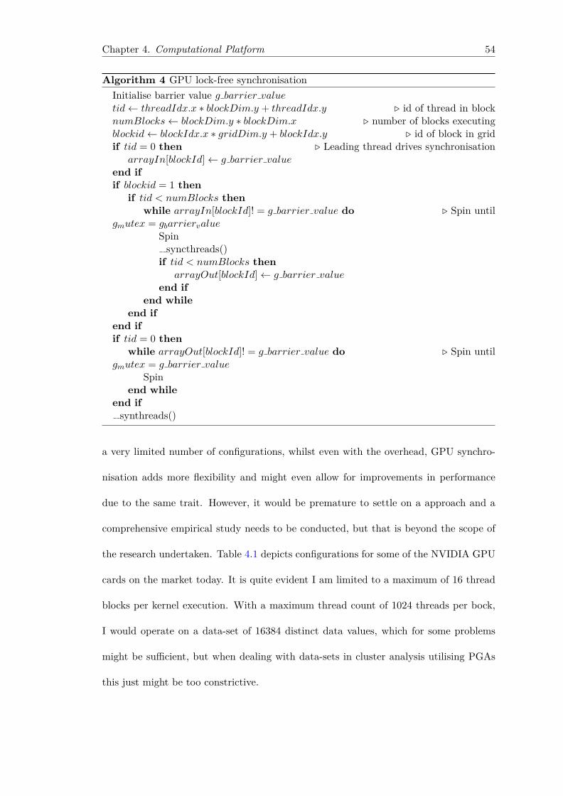
Chapter 4. Computational Platform 54
Algorithm 4 GPU lock-free synchronisationInitialise barrier value g barrier valuetid← threadIdx.x ∗ blockDim.y + threadIdx.y . id of thread in blocknumBlocks← blockDim.y ∗ blockDim.x . number of blocks executingblockid← blockIdx.x ∗ gridDim.y + blockIdx.y . id of block in gridif tid = 0 then . Leading thread drives synchronisation
arrayIn[blockId]← g barrier valueend ifif blockid = 1 then
if tid < numBlocks thenwhile arrayIn[blockId]! = g barrier value do . Spin until
gmutex = gbarriervalueSpin
syncthreads()if tid < numBlocks then
arrayOut[blockId]← g barrier valueend if
end whileend if
end ifif tid = 0 then
while arrayOut[blockId]! = g barrier value do . Spin untilgmutex = g barrier value
Spinend while
end ifsynthreads()
a very limited number of configurations, whilst even with the overhead, GPU synchro-
nisation adds more flexibility and might even allow for improvements in performance
due to the same trait. However, it would be premature to settle on a approach and a
comprehensive empirical study needs to be conducted, but that is beyond the scope of
the research undertaken. Table 4.1 depicts configurations for some of the NVIDIA GPU
cards on the market today. It is quite evident I am limited to a maximum of 16 thread
blocks per kernel execution. With a maximum thread count of 1024 threads per bock,
I would operate on a data-set of 16384 distinct data values, which for some problems
might be sufficient, but when dealing with data-sets in cluster analysis utilising PGAs
this just might be too constrictive.
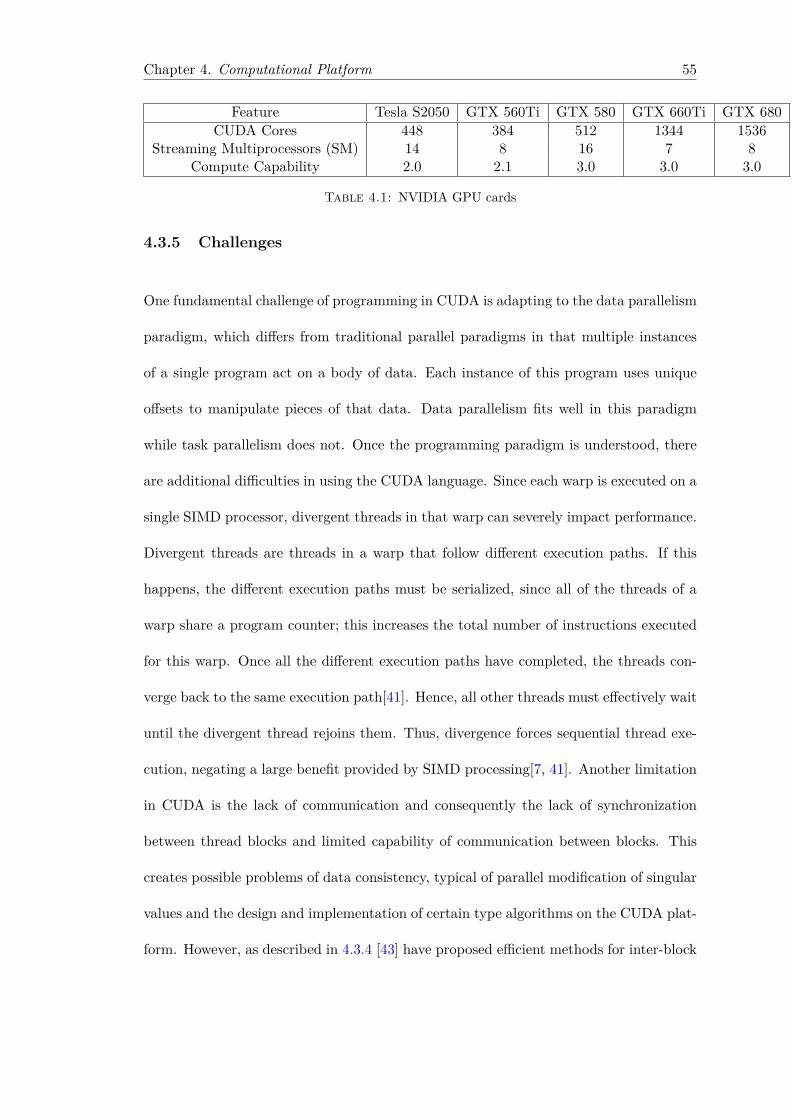
Chapter 4. Computational Platform 55
Feature Tesla S2050 GTX 560Ti GTX 580 GTX 660Ti GTX 680CUDA Cores 448 384 512 1344 1536
Streaming Multiprocessors (SM) 14 8 16 7 8Compute Capability 2.0 2.1 3.0 3.0 3.0
Table 4.1: NVIDIA GPU cards
4.3.5 Challenges
One fundamental challenge of programming in CUDA is adapting to the data parallelism
paradigm, which differs from traditional parallel paradigms in that multiple instances
of a single program act on a body of data. Each instance of this program uses unique
offsets to manipulate pieces of that data. Data parallelism fits well in this paradigm
while task parallelism does not. Once the programming paradigm is understood, there
are additional difficulties in using the CUDA language. Since each warp is executed on a
single SIMD processor, divergent threads in that warp can severely impact performance.
Divergent threads are threads in a warp that follow different execution paths. If this
happens, the different execution paths must be serialized, since all of the threads of a
warp share a program counter; this increases the total number of instructions executed
for this warp. Once all the different execution paths have completed, the threads con-
verge back to the same execution path[41]. Hence, all other threads must effectively wait
until the divergent thread rejoins them. Thus, divergence forces sequential thread exe-
cution, negating a large benefit provided by SIMD processing[7, 41]. Another limitation
in CUDA is the lack of communication and consequently the lack of synchronization
between thread blocks and limited capability of communication between blocks. This
creates possible problems of data consistency, typical of parallel modification of singular
values and the design and implementation of certain type algorithms on the CUDA plat-
form. However, as described in 4.3.4 [43] have proposed efficient methods for inter-block
Chapter 4. Computational Platform 56
communication, that does not involve transferring control over to the CPU and thus ne-
cessitating the enforcement explicit synchronisation of all the threads on the CPU. But,
on the other hand, Section 4.3.4.2 highlights the disadvantages of those inter-block com-
munication mechanisms and until such time as these have being addressed and resolved
by the NVIDIA CUDA developers, the implementation of those approaches remains
more a theoretical exercise than reality.
4.3.6 Performance tuning techniques
”We should forget about small efficiencies, say about 97% of the time: premature opti-
mization is the root of all evil” [44]. Optimising in itself is a difficult task and an even
greater task to perform on cutting-edge technology such as GPUs. The CUDA platform
features a profiling platform, which provides an invaluable tool for that task. Optimisa-
tion is a ongoing exercise, where I will have to isolate one problem area after another, in
order to attain a collective improvement in performance. The core bottlenecks for bad
performance or degradation in processing throughput on the GPU are the following:
• Kernel might be limited to instruction throughput, memory throughput or laten-
cies.
• CPU-GPU communication[42], which leads to high latency. Please refer to Section
4.3.3.3.
1. The transfer of data between the host and the device should be minimised or if
unavoidable I should rather batch small transfers into one large transfer due to the
overhead incurred with the process of initialising a CPU-device data exchange.
Chapter 4. Computational Platform 57
2. Utilise optimal kernel launch configurations in order to harness as much of the
device’s computational capability as possible.
3. Make use of asynchronous data transfers with computations. This is only possible
with the utilisation of pinned memory. Pinned memory is memory allocated on
the host, that is prevented from being swapped out and which allows for faster
transfer times between the host and the device and thus higher throughputs. Fig-
ure 4.8 depicts the timeline of execution for two code segments. In the top segment
the computation and data transfer occur in a sequential manner. In the bottom
segment concurrent copy and kernel execution allows for the overlap of kernel ex-
ecution on the device with the data transfers between the host and device. This
is only a viable option if the results can be segmented into pieces and transferred
back to the host as soon as the segment has been computed and prepared for
transfer, and I am not reliant on the computational result as a whole.
4. Avoid divergent execution paths within the same warp.
5. Minimise redundant accesses to global memory as possible. It is of paramount
importance that accesses to global memory transpire in coalesced manner, so as to
minimise the clock cycles for writes and reads as fewer transactions will be needed
to serve the thread memory access pattern. The concurrent accesses of the threads
of a warp will coalesce into a number of transactions equal to the number of cache
lines necessary to service all of the threads of the warp.
6. Optimise instruction usage by avoiding instructions that have low throughput.
This equates to trading precision over throughput and utilise single-precision over
double-precision operations.
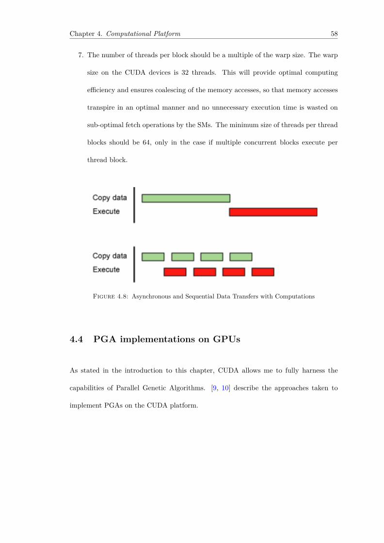
Chapter 4. Computational Platform 58
7. The number of threads per block should be a multiple of the warp size. The warp
size on the CUDA devices is 32 threads. This will provide optimal computing
efficiency and ensures coalescing of the memory accesses, so that memory accesses
transpire in an optimal manner and no unnecessary execution time is wasted on
sub-optimal fetch operations by the SMs. The minimum size of threads per thread
blocks should be 64, only in the case if multiple concurrent blocks execute per
thread block.
Figure 4.8: Asynchronous and Sequential Data Transfers with Computations
4.4 PGA implementations on GPUs
As stated in the introduction to this chapter, CUDA allows me to fully harness the
capabilities of Parallel Genetic Algorithms. [9, 10] describe the approaches taken to
implement PGAs on the CUDA platform.
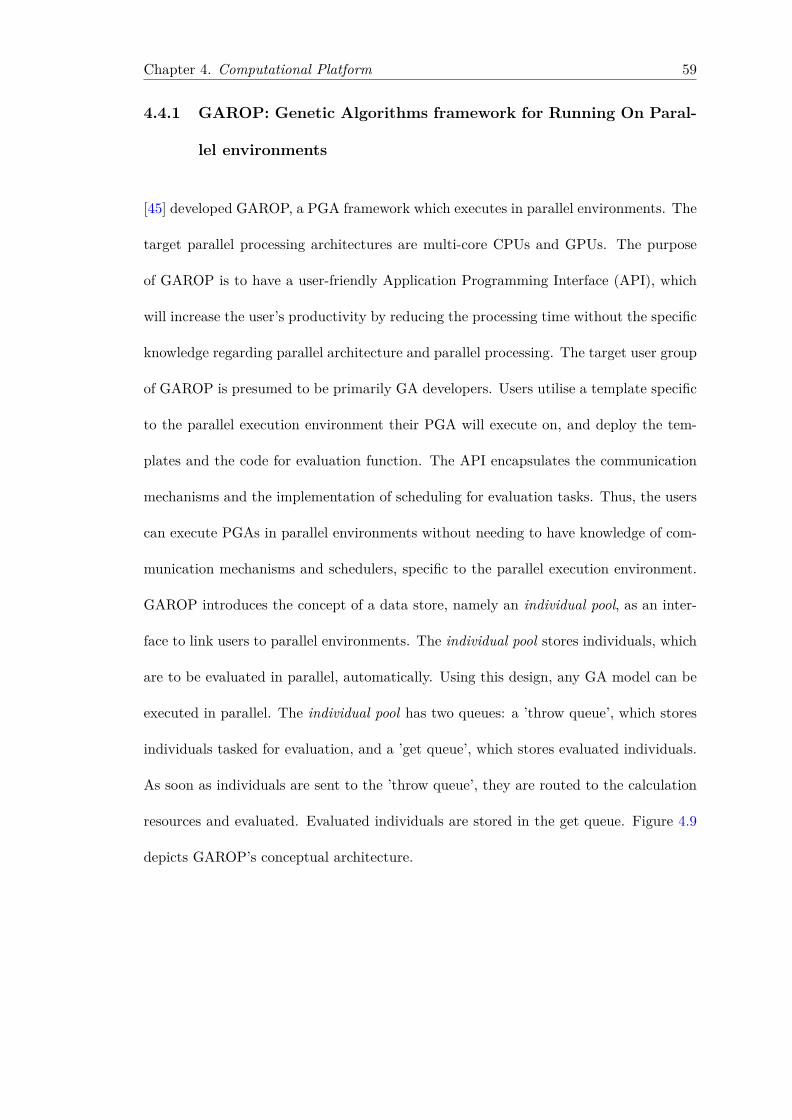
Chapter 4. Computational Platform 59
4.4.1 GAROP: Genetic Algorithms framework for Running On Paral-
lel environments
[45] developed GAROP, a PGA framework which executes in parallel environments. The
target parallel processing architectures are multi-core CPUs and GPUs. The purpose
of GAROP is to have a user-friendly Application Programming Interface (API), which
will increase the user’s productivity by reducing the processing time without the specific
knowledge regarding parallel architecture and parallel processing. The target user group
of GAROP is presumed to be primarily GA developers. Users utilise a template specific
to the parallel execution environment their PGA will execute on, and deploy the tem-
plates and the code for evaluation function. The API encapsulates the communication
mechanisms and the implementation of scheduling for evaluation tasks. Thus, the users
can execute PGAs in parallel environments without needing to have knowledge of com-
munication mechanisms and schedulers, specific to the parallel execution environment.
GAROP introduces the concept of a data store, namely an individual pool, as an inter-
face to link users to parallel environments. The individual pool stores individuals, which
are to be evaluated in parallel, automatically. Using this design, any GA model can be
executed in parallel. The individual pool has two queues: a ’throw queue’, which stores
individuals tasked for evaluation, and a ’get queue’, which stores evaluated individuals.
As soon as individuals are sent to the ’throw queue’, they are routed to the calculation
resources and evaluated. Evaluated individuals are stored in the get queue. Figure 4.9
depicts GAROP’s conceptual architecture.
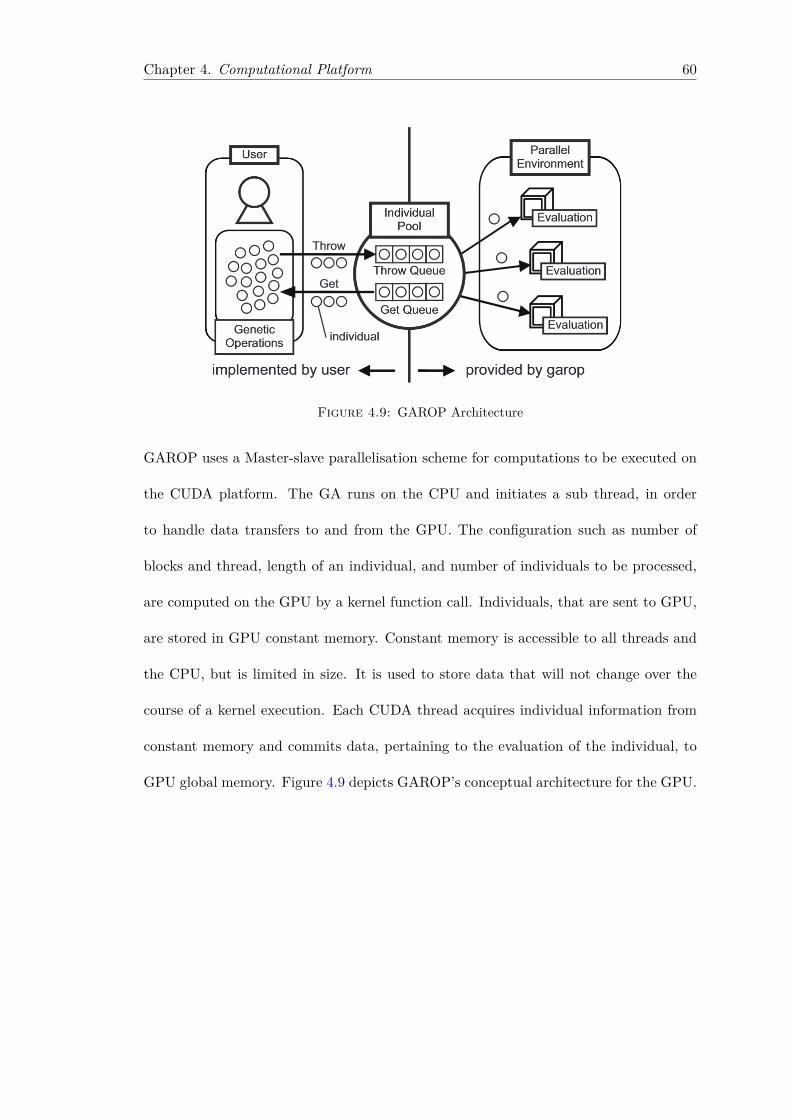
Chapter 4. Computational Platform 60
Figure 4.9: GAROP Architecture
GAROP uses a Master-slave parallelisation scheme for computations to be executed on
the CUDA platform. The GA runs on the CPU and initiates a sub thread, in order
to handle data transfers to and from the GPU. The configuration such as number of
blocks and thread, length of an individual, and number of individuals to be processed,
are computed on the GPU by a kernel function call. Individuals, that are sent to GPU,
are stored in GPU constant memory. Constant memory is accessible to all threads and
the CPU, but is limited in size. It is used to store data that will not change over the
course of a kernel execution. Each CUDA thread acquires individual information from
constant memory and commits data, pertaining to the evaluation of the individual, to
GPU global memory. Figure 4.9 depicts GAROP’s conceptual architecture for the GPU.
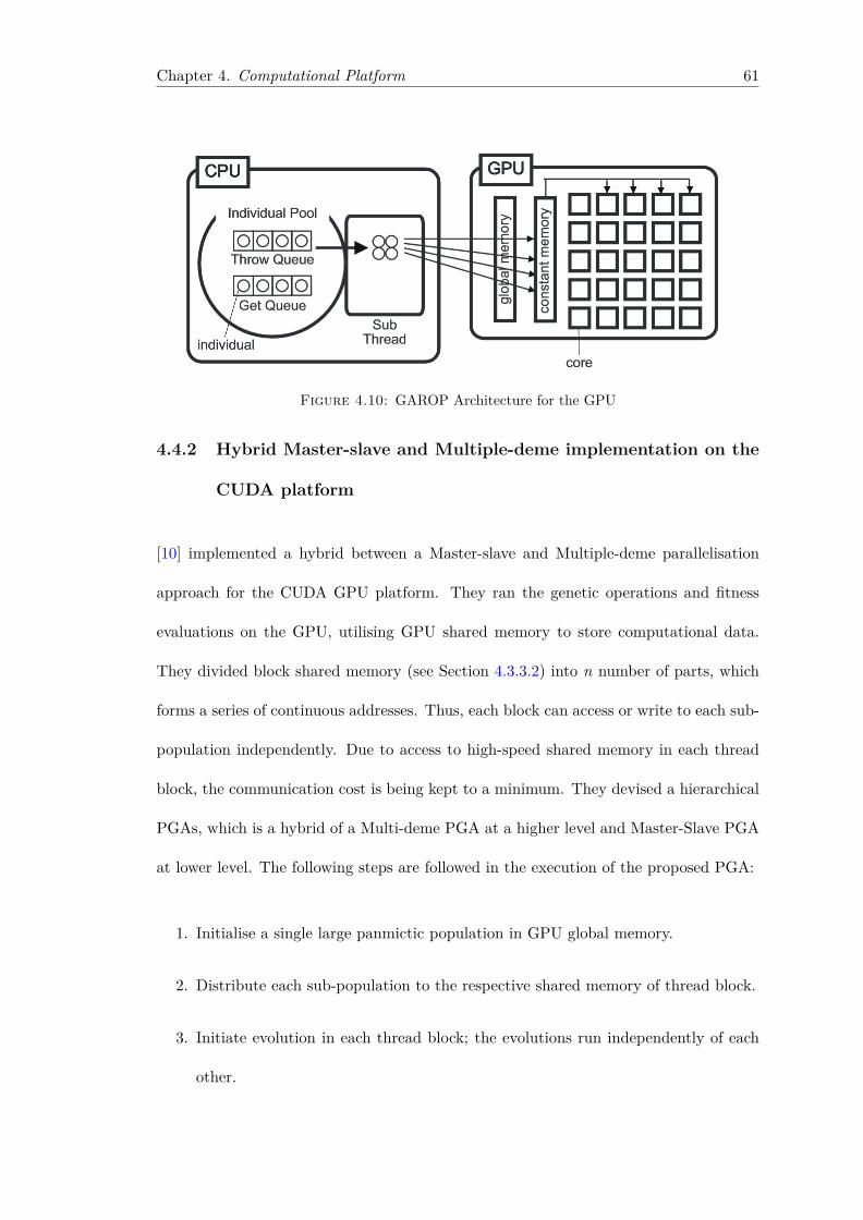
Chapter 4. Computational Platform 61
Figure 4.10: GAROP Architecture for the GPU
4.4.2 Hybrid Master-slave and Multiple-deme implementation on the
CUDA platform
[10] implemented a hybrid between a Master-slave and Multiple-deme parallelisation
approach for the CUDA GPU platform. They ran the genetic operations and fitness
evaluations on the GPU, utilising GPU shared memory to store computational data.
They divided block shared memory (see Section 4.3.3.2) into n number of parts, which
forms a series of continuous addresses. Thus, each block can access or write to each sub-
population independently. Due to access to high-speed shared memory in each thread
block, the communication cost is being kept to a minimum. They devised a hierarchical
PGAs, which is a hybrid of a Multi-deme PGA at a higher level and Master-Slave PGA
at lower level. The following steps are followed in the execution of the proposed PGA:
1. Initialise a single large panmictic population in GPU global memory.
2. Distribute each sub-population to the respective shared memory of thread block.
3. Initiate evolution in each thread block; the evolutions run independently of each
other.
Chapter 4. Computational Platform 62
Figure 4.11: Hybrid PGA CUDA architecture
4. After each evolution, initiate block exchanges of best individuals according to the
uni-directional ring migration model. See section 3.2.3.2.
5. Commit data, representing the new individual, to GPU global memory.
6. Update global memory with new individuals.
7. If termination criteria not satisfied, proceed with step 2.
Figure 4.11 depicts the architecture of the PGA implementation. The pseudo-code in
algorithm 5 illustrates the hybrid PGA.
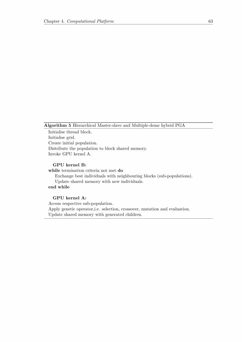
Chapter 4. Computational Platform 63
Algorithm 5 Hierarchical Master-slave and Multiple-deme hybrid PGAInitialise thread block.Initialise grid.Create initial population.Distribute the population to block shared memory.Invoke GPU kernel A.
GPU kernel B:while termination criteria not met do
Exchange best individuals with neighbouring blocks (sub-populations).Update shared memory with new individuals.
end while
GPU kernel A:Access respective sub-population.Apply genetic operator,i.e. selection, crossover, mutation and evaluation.Update shared memory with generated children.
Chapter 5
Implementation
This chapter delineates the implementation details and approach taken in implementing
a adaptive heuristic search algorithm. As presented in Chapter 2, the Master-slave and
Multiple-deme Parallelisation Schemes were chosen to search for the optimal solution to
the Giada and Marsili[11] log-likelihood function. A high-level overview of the Master-
slave algorithm implementation is presented, the various choices for the genetic operators
clearly motivated and, in succession, an overview on the approach taken to implement
the kernels and PGA cluster analysis framework on the CUDA platform, provided. A
discussion on the execution time trial methodology between the serial Matlab and the
parallelised CUDA C implementation closes off the chapter.
A Multiple-deme coarse-grained PGA, leveraging of the CUDA framework, was partially
implemented. Implementing the scheme proved to be highly complex. Unfortunately
the algorithm crashes once the different code components are assembled. Possible causes
are platform drivers and device memory conflicts. This chapter also introduces a novel
self-developed knowledge-based genetic operator that allows for highly efficient traversal
of the search space.
64
Chapter 5. Implementation 65
5.1 Stock correlation taxonomy
A number of authors[46, 47] have focused on graph-theoretical representation and anal-
ysis of the financial market. [47] focused on devising hierarchical structures in finan-
cial markets, by presenting a topological characterization of the minimal spanning tree
(MST), that can be obtained by considering the price return correlations of stocks,
traded in a financial market.[46] used correlation matrices devised from stocks in a port-
folio, by computing the synchronous time evolution of the logarithm of the difference
of the daily stock price. A spanning tree of a graph is a subgraph that contains all the
vertices and is a tree. A single graph can have many different spanning trees. A weight
is assigned to each edge and used to assign a weight to a spanning tree by computing the
sum of the weights of the edges in that spanning tree. Thus, a minimum spanning tree
(MST) is then the spanning tree with weight less than or equal to the weight of every
other spanning tree. More generally, any undirected graph, which is not necessarily
connected, has a minimum spanning forest, which is a union of minimum spanning trees
for its connected components. [46] mapped the stocks into the graph nodes and pro-
jected the relations between the stocks into the graph edges. The correlations between
the pairs of stocks are transformed into metric distances, as depicted by the following
equation:
cij =√
2 (1− ρij). (5.1)
ρij depicts the correlation value between stock i and stock j in the correlation matrix.
An application of the MST in the current financial context would denote the sum of
all weights of edges, which is minimal among all trees defined on the distance matrix.
The MSTs are visual representations of the stock correlation network, which are used
for observing, analysing and predicting stock market dynamics.
Chapter 5. Implementation 66
5.2 Approach
In this research two objectives had to fulfilled. I investigated and tuned the behaviour
of the PGA implementation using a pre-defined training set of 40 simulated stocks,
which features 4 distinct disjoint clusters. The second objective was to build a stock
correlation network based on stock price correlations, computed from the time series of
the respective securities by collecting the real-world ticker data for a pre-defined time
period from the Johannesburg Stock Exchange JSE). The approach of using a integer-
based encoding was chosen, as motivated in Section 3.1.2. The representation of the
individual is as per the Section 2.4 in Chapter 2 and looks as following:
Individual = {c1, c2, . . . , ci−1, ci} , c = 1, . . . ,K, i = 1, . . . , N. (5.2)
The variable ci is the cluster that the object i belongs to. In terms of the terminology
pertaining to Genetic Algorithms, it means that the i − th gene denotes the cluster
that i − th object or asset belongs to. The numbers of objects or assets is N . This
representation was implemented by Gebbie[12, 14] in his serial GA algorithm and was
also adopted in this research. Section 5.6.7 dissects the type of Genetic Operators used
in line with argumentation in Section 3.1.2. The fitness function will be the Giada and
Marsili maximum log-likelihood function Lc as derived in 2.4.1, which is as following:
Lc(S) = 12∑
s:ns>1[log ns
cs+ (ns − 1) log n
2s − nsn2s − cs
] (5.3)
The fitness function will be used as the measure to determine whether the cluster con-
figuration represents the inherent structure of the data set, i.e. the GA will hone in on
the fittest individual, which will represent the cluster configuration of distinct residual
Chapter 5. Implementation 67
clusters of correlated assets or objects in the data set.
The preconditioning and post-processing of the data was performed in MATLAB mak-
ing use of data pre-processing, post-processing and Minimal Spanning Tree(MST) code
libraries supplied by the supervisors for this research[48, 49]. In order to comply with
the chosen approach, I had to make modifications to the code libraries. I chose to ap-
ply the Batch Sequential Architectural Pattern[50] for the data processing. In a Batch
Sequential architecture, the task is subdivided into small processing steps, which are
implemented as separate, independent components. Each step runs to completion and
then calls the next sequential step until the whole task or job completed. During each
step a batch of data is processed and sent as a whole to the next step in form of a batch
file. The following steps are executed in order to build the stock correlation network are
in adherence with the chosen Architectural Pattern[50].
1. Precondition the data for the cluster analysis algorithm and persist the data to
batch file. This is done via the MATLAB function createRWData.m.
2. Load the preconditioned data and feed the preconditioned data into the CUDA
GA cluster analysis application and persist the data with the calculated cluster
configurations to batch file.
3. Load the cluster configurations from the batch file and feed it into the MST gen-
eration engine. Plot the generated MSTs and persist the graphical depictions as
PNG file type. This is done via the MATLAB function createMSTs.m.
4. (Alternative) Collate the plots to an AVI file.
Chapter 5. Implementation 68
5.3 Pre-processing of data for the Clustering Algorithm
In order to generate the correlation matrices for the relevant stock prices compris-
ing N stocks, the following approach was adopted: the ticker data file, serialised as
FTS(Financial Time Series) objects, is read into memory and the data conditioned.
Holes in the time series data are plugged using the Matlab function fillts() utilising a
zero-order hold interpolation approach in order to substitute missing values, denoted by
Not A Number(NaN) in the data file. Subsequently, the time series data is extracted
out of the FTS format and copied into a 2-columnar matrix, the first column containing
the ticker time values and the second column the monetary value of the stock data.
The function average() is applied to normalise the data and remove the market mode
by recursive averaging of the financial data in the matrix. Successively, I remove the
Gaussian noise from the generated covariance matrix in order to make the residual clus-
ters more pronounced thus conducting a cleansing of the correlation matrix. Random
Matrix Theory is applied in order clean the covariance matrix. The respective matrix is
decomposed and re-built via the eigenvector decomposition theorem as per the following
equation:
CorrelationMatrix = eigenvectors ∗ diag(eigenvalues) ∗ eigenvectorsT (5.4)
The sum of the eigenvalues, i.e. the variance of the system is preserved throughout the
cleansing process. The derived covariance matrix is converted into a correlation matrix,
resulting in a Hermitian matrix. The data is serialised to a text file, which is fed into the
cluster analysis PGA algorithm 5.5 for the computation of residual clusters. The cluster
configurations are then saved to a flat file for further processing and the rendering of
a graphical depiction of the financial data’s clustering characteristics using Minimum
Chapter 5. Implementation 69
Spanning Trees (MSTs), as discussed in section 5.4.
5.4 Post-processing of data and depiction of residual clus-
ters
Computed cluster configurations are read from the flat file and residual anomalies
pruned. Successively, a distance matrix is constructed by using data values from the
correlation matrix in conjunction with computed cluster configuration of the respec-
tive data set. The distance matrix is now used to construct the Minimum Spanning
Tree (MST). The MST exhibits N-1 edges, connecting the N stocks of the data set in
such a manner such that the sum of the weights of the edges is a minimum. Kruskal’s
algorithm was used to generate the MSTs, which depict the linkages between highly
correlated stocks, and in such allows me to draw observations and conclusions from it
as explained in Section 5.1.
5.5 Implementation of a Parallel Genetic Algorithm: Master-
Slave approach
As mentioned in Section 4.3 in Chapter 4, the NVIDIA CUDA platform provides key
abstractions, namely thread groups, shared memories, and barrier synchronization, ’for
fine-grained task parallelism and thread parallelism, nested within coarse-grained data
parallelism’[7]. This means, that I am afforded the capability to subdivide the task that
can undergo coarse-grained parallelism, that is tasks in which exchange of data between
processing units ensues in an infrequent manner, and most of the execution time is
devoted to processing the task or tasks at hand. Those tasks are solved independently in
Chapter 5. Implementation 70
parallel by blocks of threads, and each sub-problem into even finer units of execution that
can be solved cooperatively in parallel by all threads within the block. The primary focus
was to leverage of the CUDA’s very scalable programming model in order to parallelise
as many of the different operations of the PGA as possible so that computations would
ensue in an efficient manner.
The unparallised GA implementation of the likelihood function implemented in MAT-
LAB by Gebbie[12, 14] served as the starting point for this research. In order to max-
imise the performance of the Genetic Algorithm, the application of genetic operators and
evaluation of the fitness function were parallelised. The Master-slave PGA or Global
PGAs use a single population, where evaluation of the individuals and successive appli-
cation of genetic operators are conducted in parallel. The global parallelization model
does not predicate anything about the underlying computer architecture, so it can be
implemented efficiently on a shared-memory and distributed-memory model platform
[6]. I need to outsource as much of the GA execution to the the GPU and make use
of GPU memory as extensively as possible[10]. This allows for the minimisation of the
data transfers between the host and a device, as those transfers have a significantly
lower bandwidth than data transfers transpiring between shared or global memory and
the kernel executing on the GPU. I need to minimise and even avoid kernel accesses to
global memory [51], but this is not a viable option in this case due to the fact that I need
to utilise global memory for the storage of the population, which undergoes evolution.
The algorithm in 6 was modified in such a manner as to maximise the performance of
the Master-slave PGA and have a clear distinction between the master node, the CPU,
which controls the evolutionary process, by issuing the commands for the GA operations
to be performed on the GPU, the slave nodes or otherwise denoted the worker nodes. In
the Master-slave model, as depicted in Figure 5.1, the master, the CPU in this scenario,
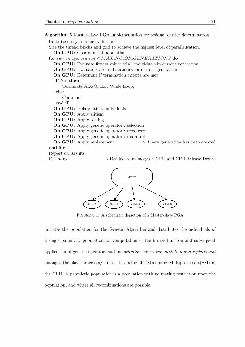
Chapter 5. Implementation 71
Algorithm 6 Master-slave PGA Implementation for residual cluster determinationInitialise ecosystem for evolutionSize the thread blocks and grid to achieve the highest level of parallelisation.
On GPU: Create initial populationfor current generation ≤MAX NO OF GENERATIONS do
On GPU: Evaluate fitness values of all individuals in current generationOn GPU: Evaluate state and statistics for current generationOn GPU: Determine if termination criteria are metif Yes then
Terminate ALGO; Exit While Loop;else
Continueend if
On GPU: Isolate fittest individualsOn GPU: Apply elitismOn GPU: Apply scalingOn GPU: Apply genetic operator : selectionOn GPU: Apply genetic operator : crossoverOn GPU: Apply genetic operator : mutationOn GPU: Apply replacement . A new generation has been created
end forReport on ResultsClean-up . Deallocate memory on GPU and CPU;Release Device
Figure 5.1: A schematic depiction of a Master-slave PGA
initiates the population for the Genetic Algorithm and distributes the individuals of
a single panmictic population for computation of the fitness function and subsequent
application of genetic operators such as selection, crossover, mutation and replacement
amongst the slave processing units, this being the Streaming Multiprocessors(SM) of
the GPU. A panmictic population is a population with no mating restriction upon the
population, and where all recombinations are possible.
Chapter 5. Implementation 72
5.6 Detailed analysis of the Parallel Genetic Algorithm:
Master-Slave approach
A sound solution design and implementation of the CUDA kernels is of paramount
importance to the successful implementation of an efficient cluster analysis algorithm.
Apart from CUDA’s Mersenne Twister implementation, the source code for the whole
cluster analysis algorithm is self-developed. Best Practices were applied consistently in
the writing of the kernels, as stipulated by Czapinski, Robilliard, Langdon, Chen, Strat-
ton and the CUDA Programming and Best Practises Guide compiled by NVIDIA[52–60].
For random number generation, I made use of CUDA’s Curand API[61] and the CUDA
Mersenne Twister implementation, opting for the latter in terms of reliability when exe-
cuting the CUDA PGA clustering application. I also made use of the CUDA THRUST
Standard Template Library(STL) [62] in order to sort, merge data and perform summa-
tion operations in the cluster analysis algorithm. CUDA THRUST Standard Template
Library(STL) is a C++ template library for CUDA based on the Standard Template
Library (STL) standard. Thrust allows me to develop high performance parallel appli-
cations with minimal programming effort through a high-level interface that wraps the
CUDA C framework.
5.6.1 Data Parallelism
Data parallelism aims at distributing the data across the fine-grained units of execution
in the most efficient manner. In the PGA implementation, the main objective was to have
a very fine-grained distribution of the population of individuals, so that I can optimally
map data elements, or the individual’s genes, to parallel processing threads[7]. As
described in Section 5.2, the individuals in the population typify a cluster configuration
Chapter 5. Implementation 73
and its representation is as following:
Individual = {c1, c2, . . . , ci−1, ci} , c = 1, . . . ,K, i = 1, . . . , N. (5.5)
The variable ci is the i − th gene which denotes the cluster that i − th object or asset
belongs to. The numbers of objects or assets is N . For example, if I had to create a
population of N = 400 individuals and was analysing the data for 16 objects or assets
the population could have the following constitution:
Individual1 = (1, 2, 4, 5, 7, 8, 2, 8, 9, 9, 1, 2, 3, 4, 5, 6)
Individual2 = (9, 2, 1, 1, 1, 3, 2, 8, 8, 8, 5, 6, 4, 3, 1, 2)
Individual3 = (3, 1, 3, 4, 6, 8, 2, 1, 1, 9, 2, 2, 2, 2, 2, 2)
Individual4 = (2, 1, 3, 3, 7, 9, 9, 1, 1, 9, 2, 2, 2, 2, 1, 1)
. . .
Individual400 = (8, 1, 9, 8, 7, 6, 5, 10, 5, 3, 6, 5, 4, 4, 3, 3)
One can envisage the population, the individuals and the genes as data on a two-
dimensional data grid. The data grid cells are mapped to threads, where each thread
executes a kernel processing the data cell at that x,y-coordinate. Thus one can envisage
the mapping as depicted in Figure 5.2.
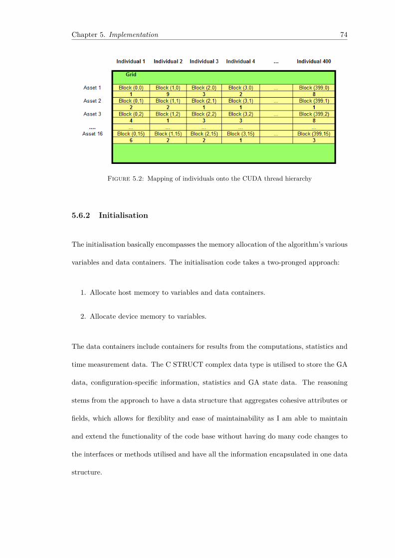
Chapter 5. Implementation 74
Figure 5.2: Mapping of individuals onto the CUDA thread hierarchy
5.6.2 Initialisation
The initialisation basically encompasses the memory allocation of the algorithm’s various
variables and data containers. The initialisation code takes a two-pronged approach:
1. Allocate host memory to variables and data containers.
2. Allocate device memory to variables.
The data containers include containers for results from the computations, statistics and
time measurement data. The C STRUCT complex data type is utilised to store the GA
data, configuration-specific information, statistics and GA state data. The reasoning
stems from the approach to have a data structure that aggregates cohesive attributes or
fields, which allows for flexiblity and ease of maintainability as I am able to maintain
and extend the functionality of the code base without having do many code changes to
the interfaces or methods utilised and have all the information encapsulated in one data
structure.
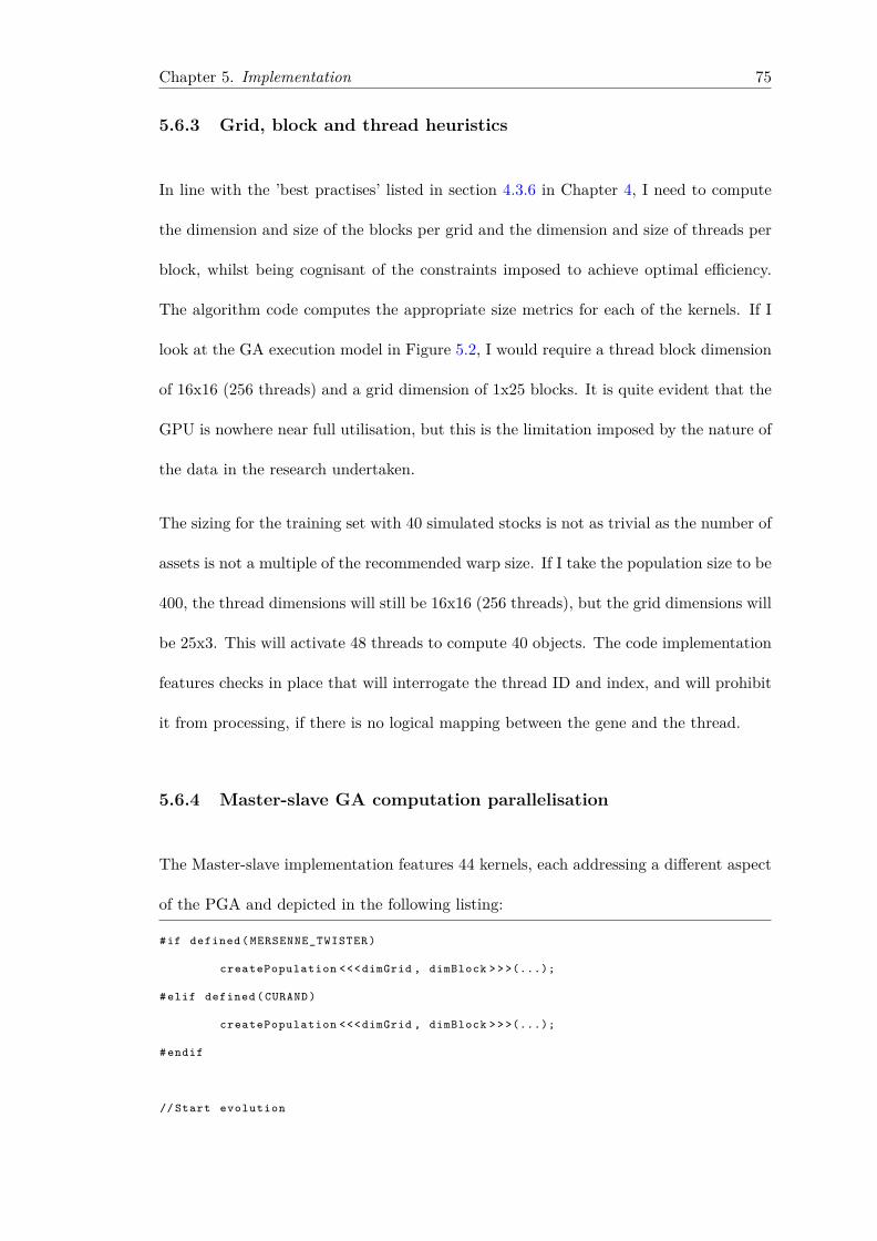
Chapter 5. Implementation 75
5.6.3 Grid, block and thread heuristics
In line with the ’best practises’ listed in section 4.3.6 in Chapter 4, I need to compute
the dimension and size of the blocks per grid and the dimension and size of threads per
block, whilst being cognisant of the constraints imposed to achieve optimal efficiency.
The algorithm code computes the appropriate size metrics for each of the kernels. If I
look at the GA execution model in Figure 5.2, I would require a thread block dimension
of 16x16 (256 threads) and a grid dimension of 1x25 blocks. It is quite evident that the
GPU is nowhere near full utilisation, but this is the limitation imposed by the nature of
the data in the research undertaken.
The sizing for the training set with 40 simulated stocks is not as trivial as the number of
assets is not a multiple of the recommended warp size. If I take the population size to be
400, the thread dimensions will still be 16x16 (256 threads), but the grid dimensions will
be 25x3. This will activate 48 threads to compute 40 objects. The code implementation
features checks in place that will interrogate the thread ID and index, and will prohibit
it from processing, if there is no logical mapping between the gene and the thread.
5.6.4 Master-slave GA computation parallelisation
The Master-slave implementation features 44 kernels, each addressing a different aspect
of the PGA and depicted in the following listing:
#if defined ( MERSENNE_TWISTER )
createPopulation <<<dimGrid , dimBlock > > >(...);
#elif defined ( CURAND )
createPopulation <<<dimGrid , dimBlock > > >(...);
# endif
// Start evolution
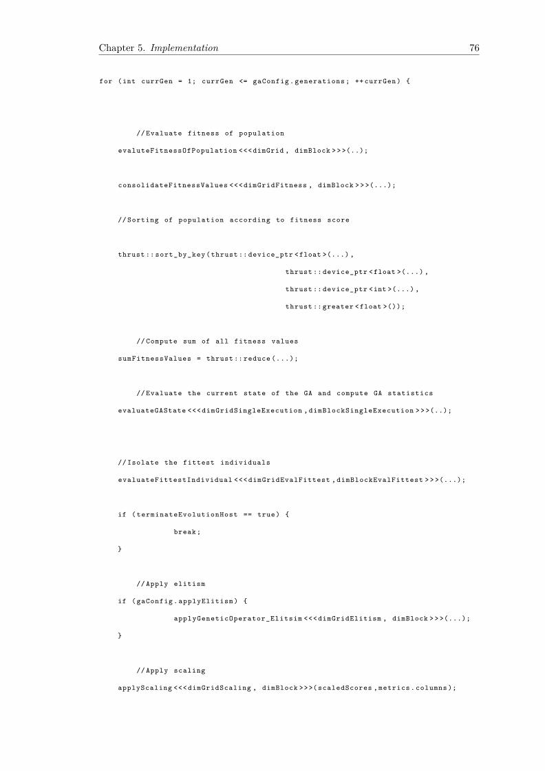
Chapter 5. Implementation 76
for (int currGen = 1; currGen <= gaConfig . generations ; ++ currGen ) {
// Evaluate fitness of population
evaluteFitnessOfPopulation <<<dimGrid , dimBlock > > >(..);
consolidateFitnessValues <<< dimGridFitness , dimBlock > > >(...);
// Sorting of population according to fitness score
thrust :: sort_by_key ( thrust :: device_ptr <float >(...) ,
thrust :: device_ptr <float >(...) ,
thrust :: device_ptr <int >(...) ,
thrust :: greater <float >());
// Compute sum of all fitness values
sumFitnessValues = thrust :: reduce (...);
// Evaluate the current state of the GA and compute GA statistics
evaluateGAState <<< dimGridSingleExecution , dimBlockSingleExecution > > >(..);
// Isolate the fittest individuals
evaluateFittestIndividual <<< dimGridEvalFittest , dimBlockEvalFittest > > >(...);
if ( terminateEvolutionHost == true) {
break ;
}
// Apply elitism
if ( gaConfig . applyElitism ) {
applyGeneticOperator_Elitsim <<< dimGridElitism , dimBlock > > >(...);
}
// Apply scaling
applyScaling <<< dimGridScaling , dimBlock >>>( scaledScores , metrics . columns );
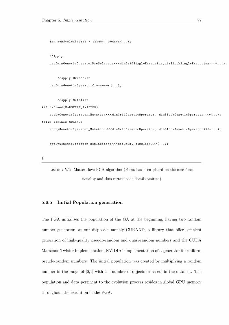
Chapter 5. Implementation 77
int sumScaledScores = thrust :: reduce (...);
// Apply
performGeneticOperatorPreSelector <<< dimGridSingleExecution , dimBlockSingleExecution > > >(...);
// Apply Crossover
performGeneticOperatorCrossover (...);
// Apply Mutation
#if defined ( MARSENNE_TWISTER )
applyGeneticOperator_Mutation <<< dimGridGeneticOperator , dimBlockGeneticOperator > > >(...);
#elif defined ( CURAND )
applyGeneticOperator_Mutation <<< dimGridGeneticOperator , dimBlockGeneticOperator > > >(...);
applyGeneticOperator_Replacement <<<dimGrid , dimBlock > > >(...);
}
Listing 5.1: Master-slave PGA algorithm (Focus has been placed on the core func-
tionality and thus certain code deatils omitted)
5.6.5 Initial Population generation
The PGA initialises the population of the GA at the beginning, having two random
number generators at our disposal: namely CURAND, a library that offers efficient
generation of high-quality pseudo-random and quasi-random numbers and the CUDA
Marsenne Twister implementation, NVIDIA’s implementation of a generator for uniform
pseudo-random numbers. The initial population was created by multiplying a random
number in the range of [0,1] with the number of objects or assets in the data-set. The
population and data pertinent to the evolution process resides in global GPU memory
throughout the execution of the PGA.
Chapter 5. Implementation 78
5.6.6 Evaluation of the fitness function
Analogous to the computation for population generation, the following computations
execute on a very fine-grained level, where each thread alloted to the computation com-
putes values for each gene in the individual or in the case of the evaluation of the fitness
value, the number of clusters K is equal to the number of objects N or the length of
chromosome. I proceed to evaluate the fitness Lc of the individuals in the population.
It is a two pass approach:
• Pass 1: Calculate the values for ns and cs for each of the clusters in each individual
by calling kernel evaluteFitnessOfPopulation().
• Pass 2: Collate the results and compute the fitness value Lc for each individual by
calling consolidateFitnessValues().
In Pass 1 the algorithm interrogates the individual and determines the number of objects
ns in each of the clusters. The kernel initialises storage in the device’s shared memory
and sums up the number of objects for each of the cluster indexes from 1, . . . , N , N
being the number of objects or the chromosome length. The cluster indices for which
there are no objects are given the value 0 and are eliminated from further computations.
Subsequently, the internal correlation cs of the cluster indices with ns > 0 is computed.
In Pass 2 the kernel reads the computed values for variables cs and ns. It filters out
the cluster indexes. Analogous, all the cluster indexes with ns = 0 are not considered,
i.e. those are indexes for clusters that are not represented in the individual depicting
a possible residual cluster configuration. This means, for example ,that Individual 2 in
Section 5.6.1 would have not have any asset or object belonging to a cluster of index 7.
Analogous to the fitness function implementation by by Gebbie[12, 14] in his serial GA
Chapter 5. Implementation 79
algorithm, I put another constraint on the permissible values for the computation. The
constraint is that if ns = 1, the value for the internal correlation must be cs < 1. If the
value is cs ≤ 1 , the the fitness value is set to 0. The algorithm then computes the value
for the Lc for all individuals in the population.
Computation of the statistics and current state of the algorithm ensues by calling the
kernel evaluateGAState(). Determination of the fittest individuals follows by comput-
ing the index of the fittest individuals within the population. In case of elitism being
applied, the fittest individuals, in number determined by configuration, are promoted
directly to the next generation. Scaling, denoted by the kernel call applyScaling() is
applied to the fitness values of the remainder of the population upon which selection of
the parents for the mating process takes place.
5.6.7 Genetic Operators and Genetic Algorithm configuration
After determining the parents’ artefacts, crossover and mutation operations ensue and
children are created that constitute the individuals of the next generation. The evolu-
tion process stops upon meeting the termination criteria for the GA. Once the optimal
individual has been determined, the data, including statistics for each of the generations,
is copied back to the host.
Genetic operators and certain Genetic Algorithm configurations are the key factors which
will determine the performance of the GA. Finding a balance between explorative and
exploitative features of GA is paramount to the success of the GA and henceforth pa-
rameter tuning of the operators and the GA configuration is unavoidable[26]. Adewumi
and Ali[26] state that this includes the tuning of parameters such as mutation probabil-
ity, the crossover operator and the population size. They also state that the parameters
Chapter 5. Implementation 80
should be dependent on the internal dynamics of the algorithm. Although the paper
by Adewumi and Ali[26] focuses on a multi-stage space allocation problem in the realm
of domain specific combinatorial optimisation problems, the methodology of tuning the
parameters is generic in nature and can be applied to any type of GA problem and
served as the basis for the PGA algorithm tuning.
5.6.7.1 Scaling
A call is issued to the kernel applyScaling() to initiate scaling on the GPU. As dis-
cussed in Section 3.1.1.1, prior to selecting the operator that will be applied to the
population, I need to adjust and scale the fitness value. The decision was taken to
opt for rank fitness scaling, analogous to the approach used by MATLAB’s GA library.
Rank fitness scaling initially adjusts the fitness value of the individuals in such a manner
that the fittest individual is assigned the value of rank 1 and the least fit the value of
P, where P is the population size. This represents the first transform. In the second
transform, the following formula is applied :
scoreIndividualn = 1RankIndividualn
, N ≤ P
This allows for full exploitation of the search space, giving all the weakest individuals
the opportunity to partake in the mating process.
5.6.7.2 Selection
A call is issued to the kernel performGeneticOperatorPreSelector() to initiate selec-
tion on the GPU. In terms of the selection approach, I applied the stochastic uniform
selection method(see Section 3.1.1.1 for description). This method provides a more
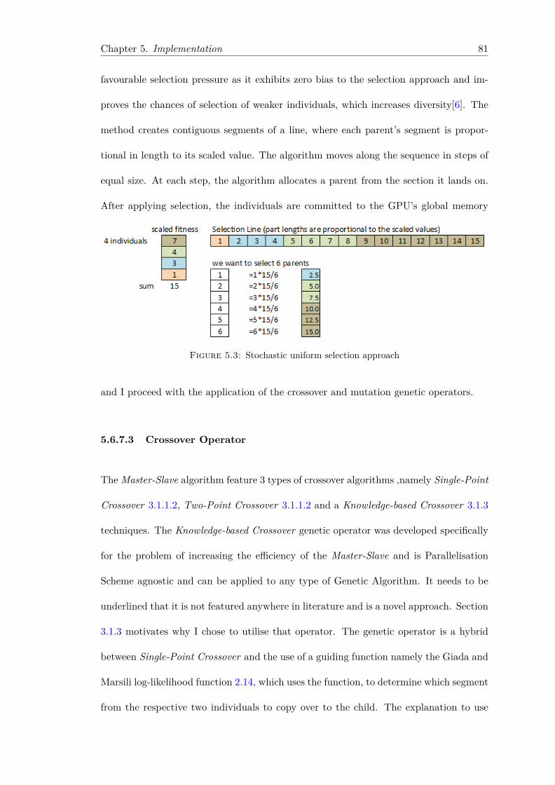
Chapter 5. Implementation 81
favourable selection pressure as it exhibits zero bias to the selection approach and im-
proves the chances of selection of weaker individuals, which increases diversity[6]. The
method creates contiguous segments of a line, where each parent’s segment is propor-
tional in length to its scaled value. The algorithm moves along the sequence in steps of
equal size. At each step, the algorithm allocates a parent from the section it lands on.
After applying selection, the individuals are committed to the GPU’s global memory
Figure 5.3: Stochastic uniform selection approach
and I proceed with the application of the crossover and mutation genetic operators.
5.6.7.3 Crossover Operator
The Master-Slave algorithm feature 3 types of crossover algorithms ,namely Single-Point
Crossover 3.1.1.2, Two-Point Crossover 3.1.1.2 and a Knowledge-based Crossover 3.1.3
techniques. The Knowledge-based Crossover genetic operator was developed specifically
for the problem of increasing the efficiency of the Master-Slave and is Parallelisation
Scheme agnostic and can be applied to any type of Genetic Algorithm. It needs to be
underlined that it is not featured anywhere in literature and is a novel approach. Section
3.1.3 motivates why I chose to utilise that operator. The genetic operator is a hybrid
between Single-Point Crossover and the use of a guiding function namely the Giada and
Marsili log-likelihood function 2.14, which uses the function, to determine which segment
from the respective two individuals to copy over to the child. The explanation to use
Chapter 5. Implementation 82
the likelihood function as described in Section2.4.1, in order to determine the ’fitter’
segment, is motivated by the fact that the application of the measure of likelihood for
cluster structure should not be restricted only to the whole data-set, but can also be
applied to subsets of data. Initially, a separate algorithm randomly determines crossover
sites for all selected parents in the population. Each parent is assigned a different locus.
Due to the nature of a Single-Point Crossover, there will be two segments per parent, a
segment left of the randomly selected crossover site and the segment right, or segment
with a starting index bigger or equal than the computed crossover site. The guiding
function is used to ascertain which of the two segments at the pre-determined loci will
be copied. A random number is generated and compared to Pcf . Should the random
number be bigger than the crossover probability, then the algorithm will copy over the
segment with the highest segment fitness value as determined by Equation 5.6, in the
event that the random value is smaller, the ’less’ fit segment is copied over, i.e. the
segment from the other individual. Two parents are selected which yield one child, that
will be injected in to the population undergoing evolution.
f = argmax‖∏→1‖
12∑
s:ns>1[log ns
cs+ (ns − 1) log n
2s − nsn2s − cs
]
(5.6)
Algorithm 7 depicts the novel Knowledge-based Crossover: The crossover operation is
initiated by the call to method performGeneticOperatorCrossover(). This in turn calls
one kernel to compute the segment scores and the other to apply the crossover operator.
5.6.7.4 Mutation Operator
Creep mutation The mutation operation is initiated by the call to method applyGeneticOperator Mutation().
Two distinct mutation operators were implemented. The first operator employs an
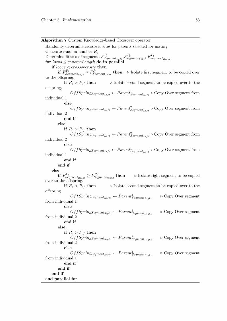
Chapter 5. Implementation 83
Algorithm 7 Custom Knowledge-based Crossover operatorRandomly determine crossover sites for parents selected for matingGenerate random number RcDetermine fitness of segments FP1
SegmentLeft,FP2segmentLeft
, FP1SegmentRight
for locus ≤ genomeLength do in parallelif locus < crossoversite then
if FP1SegmentLeft
≥ FP1SegmentLeft
then . Isolate first segment to be copied overto the offspring.
if Rc > Pcf then . Isolate second segment to be copied over to theoffspring.
OffSpringSegmentLeft← Parent1SegmentLeft
. Copy Over segment fromindividual 1
elseOffSpringSegmentLeft
← Parent2SegmentLeft. Copy Over segment from
individual 2end if
elseif Rc > Pcf then
OffSpringSegmentLeft← Parent2SegmentLeft
. Copy Over segment fromindividual 2
elseOffSpringSegmentLeft
← Parent1SegmentLeft. Copy Over segment from
individual 1end if
end ifelse
if FP1SegmentRight
≥ FP1SegmentRight
then . Isolate right segment to be copiedover to the offspring.
if Rc > Pcf then . Isolate second segment to be copied over to theoffspring.
OffSpringSegmentRight← Parent1SegmentRight
. Copy Over segmentfrom individual 1
elseOffSpringSegmentRight
← Parent2SegmentRight. Copy Over segment
from individual 2end if
elseif Rc > Pcf then
OffSpringSegmentRight← Parent2SegmentRight
. Copy Over segmentfrom individual 2
elseOffSpringSegmentRight
← Parent1SegmentRight. Copy Over segment
from individual 1end if
end ifend if
end parallel for
Chapter 5. Implementation 84
approach as utilised by [24] in a genetic algorithm-based clustering technique, called
GA-clustering, which searches for appropriate cluster centres. A number is generated
in the range between [0,1] with uniform distribution. In order to facilitate this, the
Mersenne-Twister random number generator is invoked. If the value of a gene at a
pre-defined locus is v, then the mutation approach, as depicted in 5.7 is applied to the
integer-based chromosome as following:
vt+1 =
vt ± 2 ∗ δ ∗ vt if vt 6= 0
vt ± 2 ∗ δ if vt = 0
(5.7)
5.6.7.5 Random replacement
The replacement operation is trigger by the call to method applyGeneticOperator Replacement().
The second mutation operator utilises the Mersenne-Twister random number generator
to generate a number in the range [0, 1] and multiply that number with the upper
bound value pertaining to a cluster affiliation. In the case of the training set of 40
simulated stocks, we have 40 objects, which can either belong to either a singleton or
represent 40 disjoint data points. Therefore, I would have to ensure that the generated
mutation value is within the bounds of [0,40), otherwise I would have an invalid cluster
configuration.
5.6.7.6 Replacement Operator
There are a few replacement operators, as discussed in 3.1.1.5. I chose using a weak
parent replacement scheme 3.1.1.5, where the stronger parent and the offspring are
promoted to the next phase of evolution. This introduces bias towards fitter individuals,
Chapter 5. Implementation 85
thus increasing the overall fitness of the population, but reduces the diversity of the
mating pool.
5.6.8 Termination Criteria
There are two significant termination criteria, namely
• Once a pre-defined number of maximum evolutions has been executed, the algo-
rithm terminates.
• If there is no notable improvement in the fitness value of the fittest individual,
representing the most optimal cluster configuration resident in the data-set being
analysed, the algorithm will continue to iterate through a pre-defined number
of evolutions, denoted stall generations Gstall. The fittest individual from the
previous evolution is compared to the fittest individual of the current evolution
and if the difference between the two values is smaller than a pre-defined error
tolerance, one would classify this as a stall generation.
5.7 Parallel Genetic Algorithm tuning
In order to ensure an efficient implementation of the Master-slave algorithm, I need to
find a balance between exploration of the search space and exploitation of the discoveries
in the search space. The more exploitation of the discoveries that is made, the faster the
PGA will converge towards a solution, but will fail at finding the true global optimum.
The more exploration will lead to finding the true optimum, but will slow down conver-
gence. I opted for tuning the mutation probability, the crossover operator parameter and
the population size, analogous to the approach taken and motivated by Adewumi and
Chapter 5. Implementation 86
Ali[26]. I additionally looked at finding an efficient mutation operator, finding an ideal
setting for the novel and self-developed knowledge-based crossover operator (see Section
5.6.7.3) and at tuning the number of elite individuals that get promoted to the next
generation. The following algorithm parameter tuning experiments were compiled in
order to arrive at the optimal algorithm configuration settings, as the PGA parameters
affect the algorithms search quality and efficiency[30]:
• Investigation into the effect of population size on the efficiency of the PGA
• Investigation into the effect of crossover probability Pc on the efficiency of the
PGA
• Investigation into the effect of crossover probability Pc on the efficiency of the
PGA
• Investigation into the effect of mutation probability Pm on the efficiency of the
PGA
• Investigation into the effect of knowledge-based crossover fragment operator prob-
ability Pcf on the efficiency of the PGA
• Investigation into the effect of crossover genetic operator on the efficiency of the
PGA
• Investigation into the effect of mutation genetic operator on the efficiency of the
PGA
• Investigation into the effect of the number of elite individuals promoted to the
next generation on the efficiency of the PGA.
Chapter 5. Implementation 87
5.8 Measurement metrics
The tuning exercise was performed on the training set of 4 disjoint clusters and in such
it represents the optimal GA parameters for the training set data set.
5.8.1 Performance metric
In order to analyse the efficiency of an algorithm, I would usually apply time complexity
analysis to get an estimate of the running time as a function of the size of the input data.
This result is normally expressed using Big O notation. This is useful for comparing
algorithms in cases where a large amount of data is to processed, which is not the case
in this research. This research focuses on a small set of data-and the goal of returning
a result in the shortest possible time. This will in turn lead to faster computation
of high-frequency, low-latency data feeds, where a high throughput of data needs to
be processed efficiently. Secondly, algorithms which include parallel processing may
be more difficult to analyse using the Big O notation. Thus, in order to be able to
measure the efficiency of the algorithm, measurements of the time taken to execute a
clustering analysis on a data set were conducted. Two common time measures are: CPU
time and Elapsed time. CPU time is the actual time it takes the Central Processing Unit
(CPU) to process the instructions of a computer program or the Operating System (OS).
This does not include the waiting for Input/Output resources (I/O) to complete their
operations or the context switching operations in the OS. The Elapsed time measures
the total time pertaining to the execution of a computer program, which means the
duration from when the process was started until the time it terminated. Execution
time trails of each of the implementations were executed. The decision was taken to use
the elapsed time as a benchmarking metric. It is quite an involved process to be able to
Chapter 5. Implementation 88
compare computational times for an algorithm that can both run on a CPU and a GPU
and in such somehow try to quantify its efficiency. The CUDA framework provides a
profiling workbench, which reports benchmarking metrics to a fine level of granularity.
It will report on CPU and GPU time spent on executing a piece of CUDA code and for
example, on the time taken to for transfer of data between the host and device; such a
level of detail is beyond the scope of this research. I rather opted for introducing time
measuring barriers, localised in such places in the code base so that they give a good
enough indication as to the execution times of the different manifestations of a PGAs run
on various platforms under different configurations and run on multiple environments
as listed in Section 6.1.
5.8.2 Average calculations
Algorithm tuning experiments described in Section 6.2.2 employed the calculation of
the arithmetic average value for the fitness of all individuals in the population for that
generation, which was calculated in the following manner: Fave = 1n
∑Ni=1 Findividual,
where n denotes the number of the individuals, Fave the average fitness and Findividual
the respective fitness value of the individual. This metric will indicate the quality of the
successive population of individuals generated by the PGA.
Chapter 6
Experiments and Measurements
This chapter reports on the algorithm tuning and execution time trials of the CUDA
PGA implementation being executed on two OS platforms, and against the serial GA
implementation[14]. The following algorithm parameter tuning experiments were com-
piled in order to arrive at the optimal algorithm configuration settings as described and
motivated in Section 5.7:
• Investigation into the effect of population size on the efficiency of the PGA.
• Investigation into the effect of crossover probability Pc on the efficiency of the
PGA.
• Investigation into the effect of crossover probability Pc on the efficiency of the
PGA.
• Investigation into the effect of mutation probability Pm on the efficiency of the
PGA.
• Investigation into the effect of knowledge-based crossover fragment operator prob-
ability Pcf on the efficiency of the PGA.
89
Chapter 6. Results and Discussion 90
• Investigation into the effect of crossover genetic operator on the efficiency of the
PGA.
• Investigation into the effect of mutation genetic operator on the efficiency of the
PGA.
• Investigation into the effect of the number of elite individuals promoted to the
next generation on the efficiency of the PGA.
It also presents clustering analysis results, depicted in the form of Minimum Spanning
Trees, as described in Section 5.1, of 1780 time units of real-word stock prices taken
from the Johannesburg Stock Exchange(JSE) spanning over the time period from 28th
September 2012 until 10th of October 2012.
6.1 Environment
The CUDA algorithm and the respective test harness were primarily developed on the
Linux platform. It was successively ported to the Windows environment. Multiple en-
vironments were configured as per the configuration depicted in Table 6.1 in order to
provide a high-level overview of the versatility of the CUDA cluster analysis algorithm
and highlight that its efficiency is not confined to one platform and thus is platform-
independent. All the CUDA code was compiled with the the CUDA C compiler nvcc,
version 5.0. The code was compiled against two configuration sets, namely the DEBUG
configuration for debugging and testing, and a RELEASE configuration, optimised to
perform code execution time measurements. The code was compiled with CUDA com-
pute capabilities of 2.0 and 3.0. The CUDA compute capability designates a ’feature set’,
being both software and hardware features, that a device supports. In the RELEASE
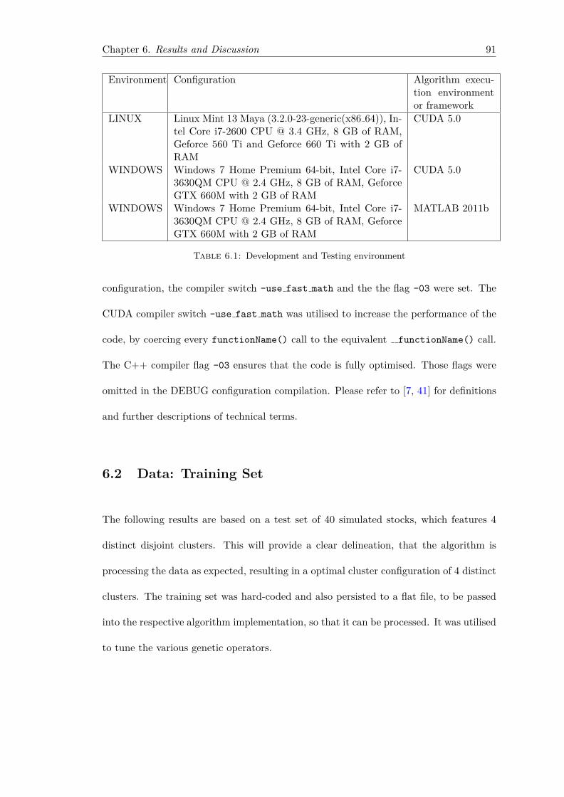
Chapter 6. Results and Discussion 91
Environment Configuration Algorithm execu-tion environmentor framework
LINUX Linux Mint 13 Maya (3.2.0-23-generic(x86 64)), In-tel Core i7-2600 CPU @ 3.4 GHz, 8 GB of RAM,Geforce 560 Ti and Geforce 660 Ti with 2 GB ofRAM
CUDA 5.0
WINDOWS Windows 7 Home Premium 64-bit, Intel Core i7-3630QM CPU @ 2.4 GHz, 8 GB of RAM, GeforceGTX 660M with 2 GB of RAM
CUDA 5.0
WINDOWS Windows 7 Home Premium 64-bit, Intel Core i7-3630QM CPU @ 2.4 GHz, 8 GB of RAM, GeforceGTX 660M with 2 GB of RAM
MATLAB 2011b
Table 6.1: Development and Testing environment
configuration, the compiler switch -use fast math and the the flag -03 were set. The
CUDA compiler switch -use fast math was utilised to increase the performance of the
code, by coercing every functionName() call to the equivalent functionName() call.
The C++ compiler flag -03 ensures that the code is fully optimised. Those flags were
omitted in the DEBUG configuration compilation. Please refer to [7, 41] for definitions
and further descriptions of technical terms.
6.2 Data: Training Set
The following results are based on a test set of 40 simulated stocks, which features 4
distinct disjoint clusters. This will provide a clear delineation, that the algorithm is
processing the data as expected, resulting in a optimal cluster configuration of 4 distinct
clusters. The training set was hard-coded and also persisted to a flat file, to be passed
into the respective algorithm implementation, so that it can be processed. It was utilised
to tune the various genetic operators.
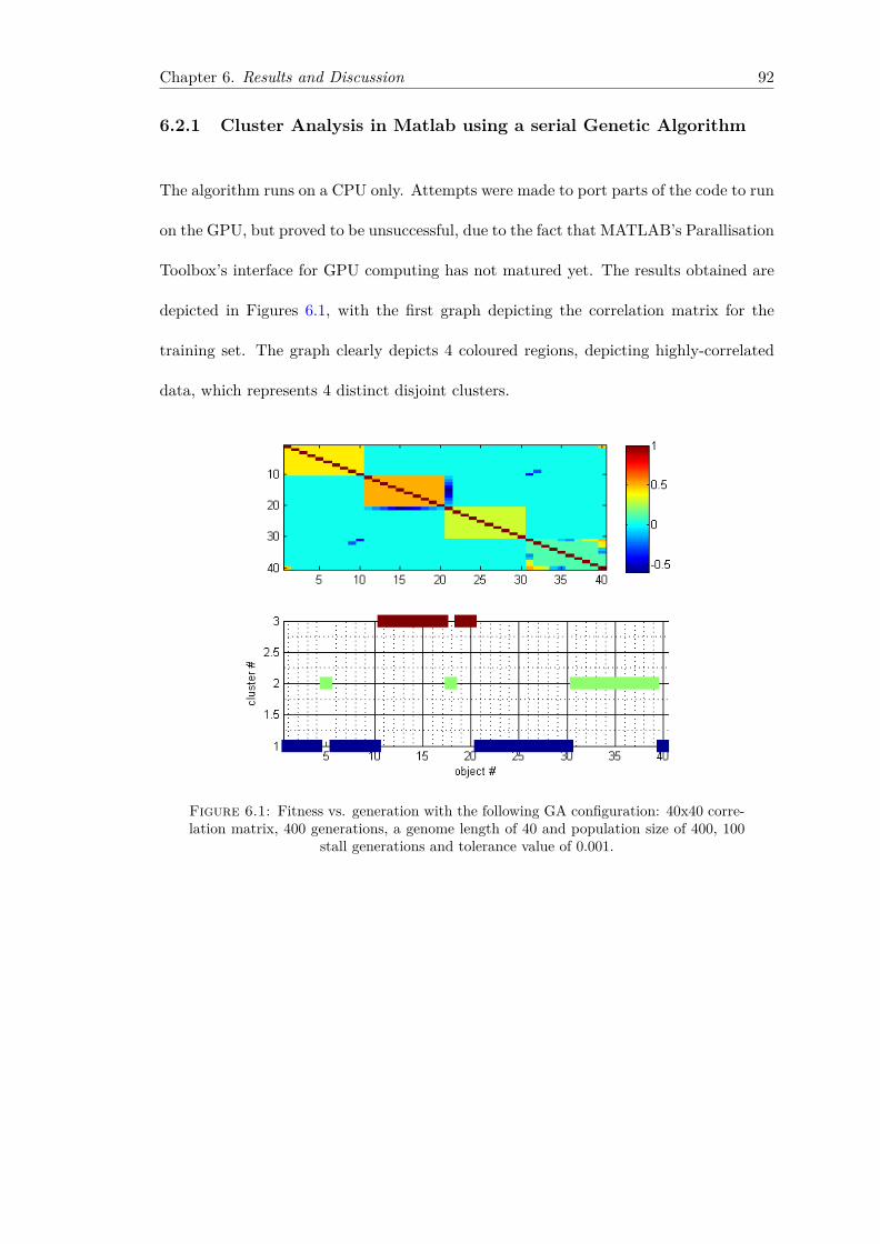
Chapter 6. Results and Discussion 92
6.2.1 Cluster Analysis in Matlab using a serial Genetic Algorithm
The algorithm runs on a CPU only. Attempts were made to port parts of the code to run
on the GPU, but proved to be unsuccessful, due to the fact that MATLAB’s Parallisation
Toolbox’s interface for GPU computing has not matured yet. The results obtained are
depicted in Figures 6.1, with the first graph depicting the correlation matrix for the
training set. The graph clearly depicts 4 coloured regions, depicting highly-correlated
data, which represents 4 distinct disjoint clusters.
Figure 6.1: Fitness vs. generation with the following GA configuration: 40x40 corre-lation matrix, 400 generations, a genome length of 40 and population size of 400, 100
stall generations and tolerance value of 0.001.
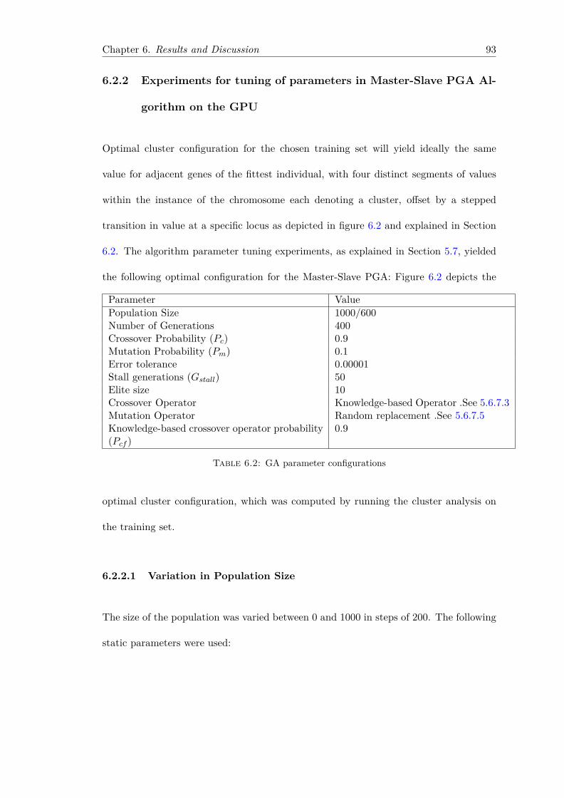
Chapter 6. Results and Discussion 93
6.2.2 Experiments for tuning of parameters in Master-Slave PGA Al-
gorithm on the GPU
Optimal cluster configuration for the chosen training set will yield ideally the same
value for adjacent genes of the fittest individual, with four distinct segments of values
within the instance of the chromosome each denoting a cluster, offset by a stepped
transition in value at a specific locus as depicted in figure 6.2 and explained in Section
6.2. The algorithm parameter tuning experiments, as explained in Section 5.7, yielded
the following optimal configuration for the Master-Slave PGA: Figure 6.2 depicts the
Parameter ValuePopulation Size 1000/600Number of Generations 400Crossover Probability (Pc) 0.9Mutation Probability (Pm) 0.1Error tolerance 0.00001Stall generations (Gstall) 50Elite size 10Crossover Operator Knowledge-based Operator .See 5.6.7.3Mutation Operator Random replacement .See 5.6.7.5Knowledge-based crossover operator probability(Pcf )
0.9
Table 6.2: GA parameter configurations
optimal cluster configuration, which was computed by running the cluster analysis on
the training set.
6.2.2.1 Variation in Population Size
The size of the population was varied between 0 and 1000 in steps of 200. The following
static parameters were used:
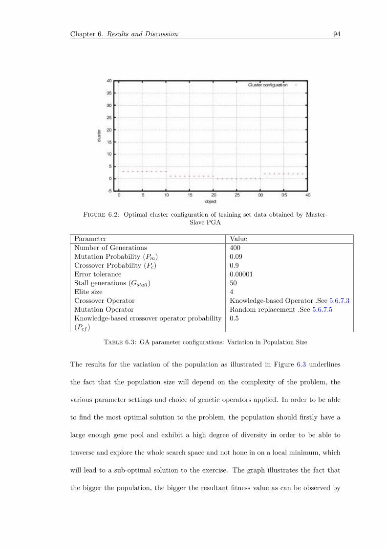
Chapter 6. Results and Discussion 94
Figure 6.2: Optimal cluster configuration of training set data obtained by Master-Slave PGA
Parameter ValueNumber of Generations 400Mutation Probability (Pm) 0.09Crossover Probability (Pc) 0.9Error tolerance 0.00001Stall generations (Gstall) 50Elite size 4Crossover Operator Knowledge-based Operator .See 5.6.7.3Mutation Operator Random replacement .See 5.6.7.5Knowledge-based crossover operator probability(Pcf )
0.5
Table 6.3: GA parameter configurations: Variation in Population Size
The results for the variation of the population as illustrated in Figure 6.3 underlines
the fact that the population size will depend on the complexity of the problem, the
various parameter settings and choice of genetic operators applied. In order to be able
to find the most optimal solution to the problem, the population should firstly have a
large enough gene pool and exhibit a high degree of diversity in order to be able to
traverse and explore the whole search space and not hone in on a local minimum, which
will lead to a sub-optimal solution to the exercise. The graph illustrates the fact that
the bigger the population, the bigger the resultant fitness value as can be observed by
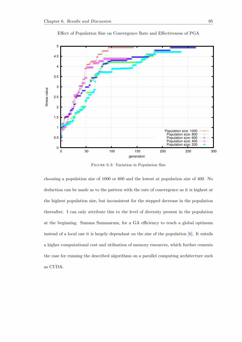
Chapter 6. Results and Discussion 95
Effect of Population Size on Convergence Rate and Effectiveness of PGA
0
0.5
1
1.5
2
2.5
3
3.5
4
4.5
5
0 50 100 150 200 250 300
fitn
ess v
alu
e
generation
Population size: 1000Population size: 800Population size: 600Population size: 400Population size: 200
Figure 6.3: Variation in Population Size
choosing a population size of 1000 or 600 and the lowest at population size of 400. No
deduction can be made as to the pattern with the rate of convergence as it is highest at
the highest population size, but inconsistent for the stepped decrease in the population
thereafter. I can only attribute this to the level of diversity present in the population
at the beginning. Summa Summarum, for a GA efficiency to reach a global optimum
instead of a local one it is largely dependant on the size of the population [6]. It entails
a higher computational cost and utilisation of memory resources, which further cements
the case for running the described algorithms on a parallel computing architecture such
as CUDA.
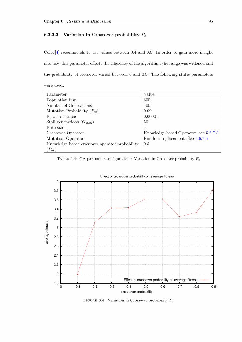
Chapter 6. Results and Discussion 96
6.2.2.2 Variation in Crossover probability Pc
Coley[4] recommends to use values between 0.4 and 0.9. In order to gain more insight
into how this parameter effects the efficiency of the algorithm, the range was widened and
the probability of crossover varied between 0 and 0.9. The following static parameters
were used:
Parameter ValuePopulation Size 600Number of Generations 400Mutation Probability (Pm) 0.09Error tolerance 0.00001Stall generations (Gstall) 50Elite size 4Crossover Operator Knowledge-based Operator .See 5.6.7.3Mutation Operator Random replacement .See 5.6.7.5Knowledge-based crossover operator probability(Pcf )
0.5
Table 6.4: GA parameter configurations: Variation in Crossover probability Pc
1.8
2
2.2
2.4
2.6
2.8
3
3.2
3.4
3.6
3.8
4
0 0.1 0.2 0.3 0.4 0.5 0.6 0.7 0.8 0.9
ave
rag
e f
itn
ess
crossover probability
Effect of crossover probability on average fitness
Effect of crossover probability on average fitness
Figure 6.4: Variation in Crossover probability Pc
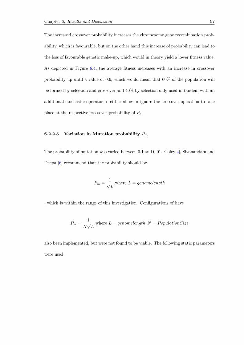
Chapter 6. Results and Discussion 97
The increased crossover probability increases the chromosome gene recombination prob-
ability, which is favourable, but on the other hand this increase of probability can lead to
the loss of favourable genetic make-up, which would in theory yield a lower fitness value.
As depicted in Figure 6.4, the average fitness increases with an increase in crossover
probability up until a value of 0.6, which would mean that 60% of the population will
be formed by selection and crossover and 40% by selection only used in tandem with an
additional stochastic operator to either allow or ignore the crossover operation to take
place at the respective crossover probability of Pc.
6.2.2.3 Variation in Mutation probability Pm
The probability of mutation was varied between 0.1 and 0.01. Coley[4], Sivanandam and
Deepa [6] recommend that the probability should be
Pm = 1√L
,where L = genomelength
, which is within the range of this investigation. Configurations of have
Pm = 1N√L
,where L = genomelength,N = PopulationSize
also been implemented, but were not found to be viable. The following static parameters
were used:
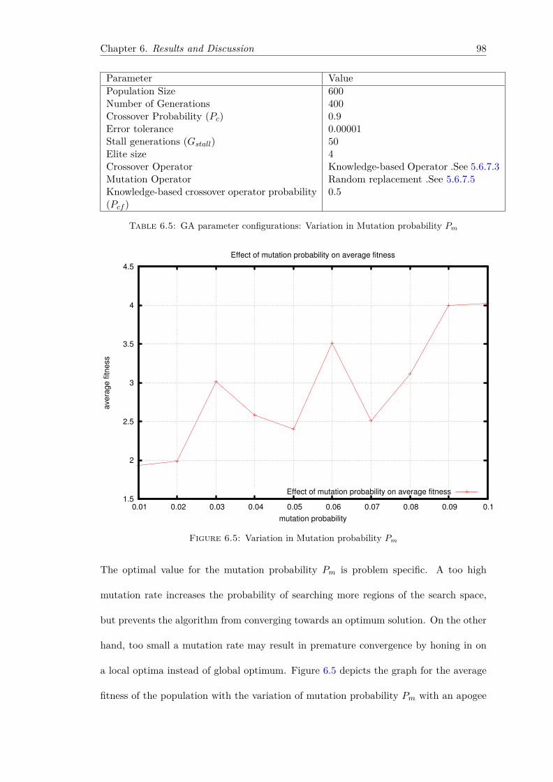
Chapter 6. Results and Discussion 98
Parameter ValuePopulation Size 600Number of Generations 400Crossover Probability (Pc) 0.9Error tolerance 0.00001Stall generations (Gstall) 50Elite size 4Crossover Operator Knowledge-based Operator .See 5.6.7.3Mutation Operator Random replacement .See 5.6.7.5Knowledge-based crossover operator probability(Pcf )
0.5
Table 6.5: GA parameter configurations: Variation in Mutation probability Pm
1.5
2
2.5
3
3.5
4
4.5
0.01 0.02 0.03 0.04 0.05 0.06 0.07 0.08 0.09 0.1
ave
rag
e f
itn
ess
mutation probability
Effect of mutation probability on average fitness
Effect of mutation probability on average fitness
Figure 6.5: Variation in Mutation probability Pm
The optimal value for the mutation probability Pm is problem specific. A too high
mutation rate increases the probability of searching more regions of the search space,
but prevents the algorithm from converging towards an optimum solution. On the other
hand, too small a mutation rate may result in premature convergence by honing in on
a local optima instead of global optimum. Figure 6.5 depicts the graph for the average
fitness of the population with the variation of mutation probability Pm with an apogee
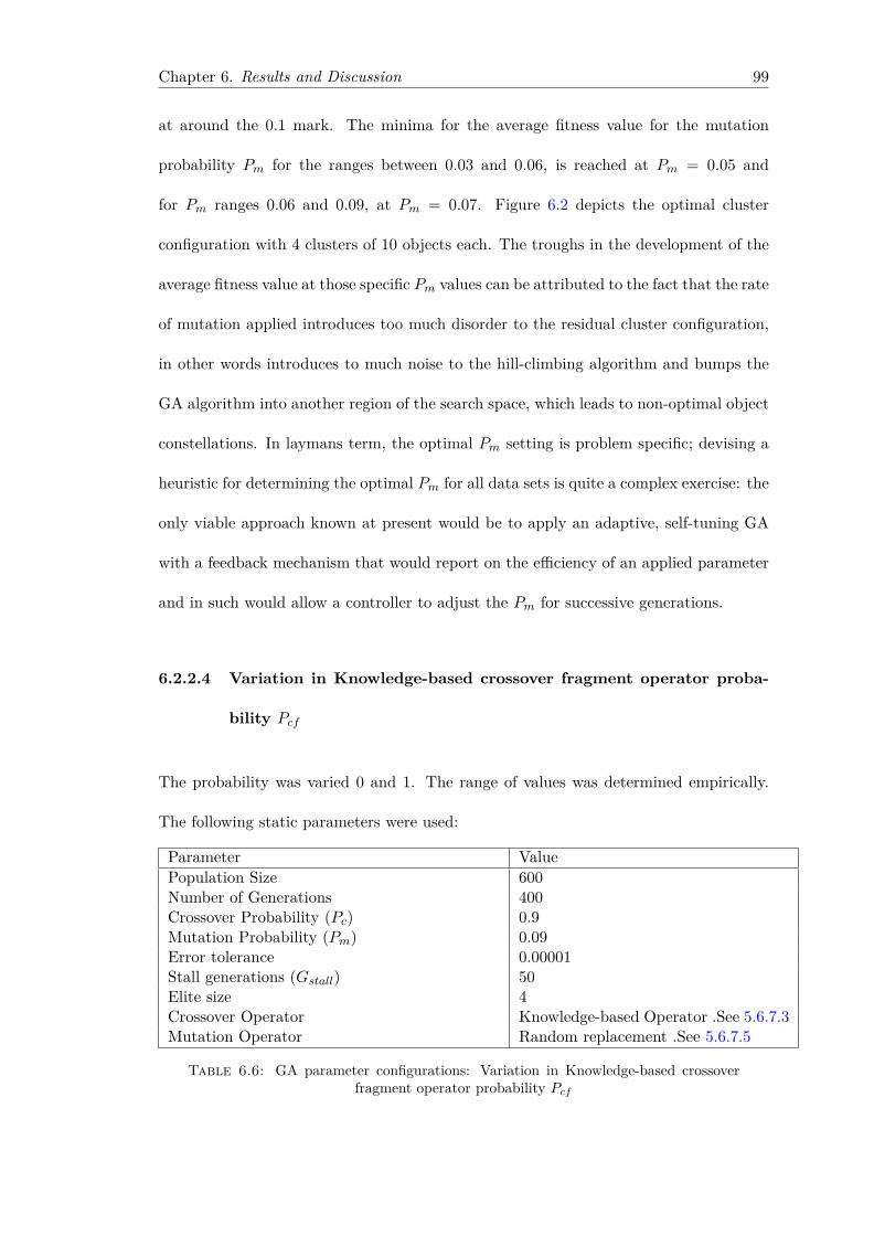
Chapter 6. Results and Discussion 99
at around the 0.1 mark. The minima for the average fitness value for the mutation
probability Pm for the ranges between 0.03 and 0.06, is reached at Pm = 0.05 and
for Pm ranges 0.06 and 0.09, at Pm = 0.07. Figure 6.2 depicts the optimal cluster
configuration with 4 clusters of 10 objects each. The troughs in the development of the
average fitness value at those specific Pm values can be attributed to the fact that the rate
of mutation applied introduces too much disorder to the residual cluster configuration,
in other words introduces to much noise to the hill-climbing algorithm and bumps the
GA algorithm into another region of the search space, which leads to non-optimal object
constellations. In laymans term, the optimal Pm setting is problem specific; devising a
heuristic for determining the optimal Pm for all data sets is quite a complex exercise: the
only viable approach known at present would be to apply an adaptive, self-tuning GA
with a feedback mechanism that would report on the efficiency of an applied parameter
and in such would allow a controller to adjust the Pm for successive generations.
6.2.2.4 Variation in Knowledge-based crossover fragment operator proba-
bility Pcf
The probability was varied 0 and 1. The range of values was determined empirically.
The following static parameters were used:
Parameter ValuePopulation Size 600Number of Generations 400Crossover Probability (Pc) 0.9Mutation Probability (Pm) 0.09Error tolerance 0.00001Stall generations (Gstall) 50Elite size 4Crossover Operator Knowledge-based Operator .See 5.6.7.3Mutation Operator Random replacement .See 5.6.7.5
Table 6.6: GA parameter configurations: Variation in Knowledge-based crossoverfragment operator probability Pcf
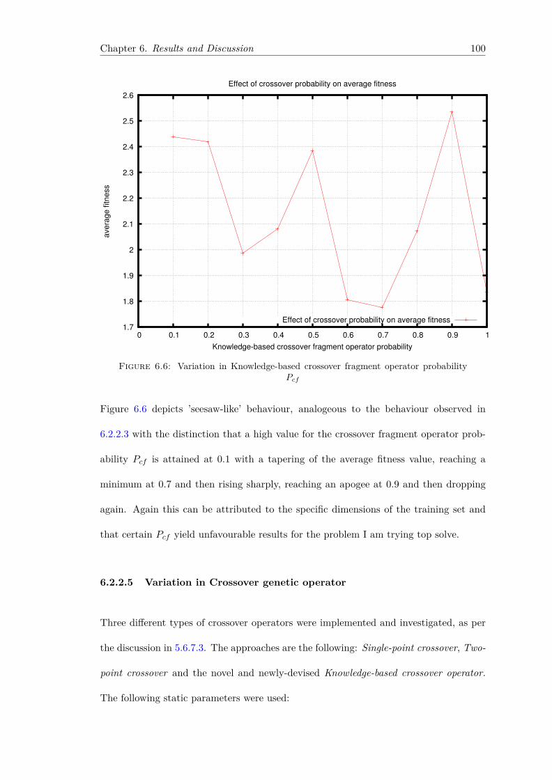
Chapter 6. Results and Discussion 100
1.7
1.8
1.9
2
2.1
2.2
2.3
2.4
2.5
2.6
0 0.1 0.2 0.3 0.4 0.5 0.6 0.7 0.8 0.9 1
ave
rag
e f
itn
ess
Knowledge-based crossover fragment operator probability
Effect of crossover probability on average fitness
Effect of crossover probability on average fitness
Figure 6.6: Variation in Knowledge-based crossover fragment operator probabilityPcf
Figure 6.6 depicts ’seesaw-like’ behaviour, analogeous to the behaviour observed in
6.2.2.3 with the distinction that a high value for the crossover fragment operator prob-
ability Pcf is attained at 0.1 with a tapering of the average fitness value, reaching a
minimum at 0.7 and then rising sharply, reaching an apogee at 0.9 and then dropping
again. Again this can be attributed to the specific dimensions of the training set and
that certain Pcf yield unfavourable results for the problem I am trying top solve.
6.2.2.5 Variation in Crossover genetic operator
Three different types of crossover operators were implemented and investigated, as per
the discussion in 5.6.7.3. The approaches are the following: Single-point crossover, Two-
point crossover and the novel and newly-devised Knowledge-based crossover operator.
The following static parameters were used:
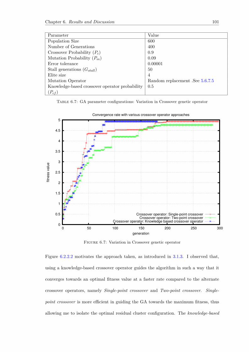
Chapter 6. Results and Discussion 101
Parameter ValuePopulation Size 600Number of Generations 400Crossover Probability (Pc) 0.9Mutation Probability (Pm) 0.09Error tolerance 0.00001Stall generations (Gstall) 50Elite size 4Mutation Operator Random replacement .See 5.6.7.5Knowledge-based crossover operator probability(Pcf )
0.5
Table 6.7: GA parameter configurations: Variation in Crossover genetic operator
0
0.5
1
1.5
2
2.5
3
3.5
4
4.5
5
0 50 100 150 200 250 300
fitn
ess v
alu
e
generation
Convergence rate with various crossover operator approaches
Crossover operator: Single-point crossoverCrossover operator: Two-point crossover
Crossover operator: Knowledge based crossover operator
Figure 6.7: Variation in Crossover genetic operator
Figure 6.2.2.2 motivates the approach taken, as introduced in 3.1.3. I observed that,
using a knowledge-based crossover operator guides the algorithm in such a way that it
converges towards an optimal fitness value at a faster rate compared to the alternate
crossover operators, namely Single-point crossover and Two-point crossover. Single-
point crossover is more efficient in guiding the GA towards the maximum fitness, thus
allowing me to isolate the optimal residual cluster configuration. The knowledge-based
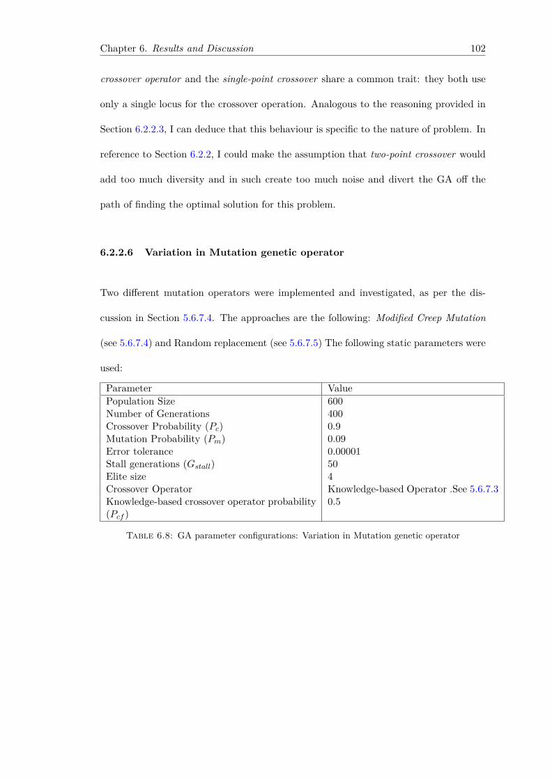
Chapter 6. Results and Discussion 102
crossover operator and the single-point crossover share a common trait: they both use
only a single locus for the crossover operation. Analogous to the reasoning provided in
Section 6.2.2.3, I can deduce that this behaviour is specific to the nature of problem. In
reference to Section 6.2.2, I could make the assumption that two-point crossover would
add too much diversity and in such create too much noise and divert the GA off the
path of finding the optimal solution for this problem.
6.2.2.6 Variation in Mutation genetic operator
Two different mutation operators were implemented and investigated, as per the dis-
cussion in Section 5.6.7.4. The approaches are the following: Modified Creep Mutation
(see 5.6.7.4) and Random replacement (see 5.6.7.5) The following static parameters were
used:
Parameter ValuePopulation Size 600Number of Generations 400Crossover Probability (Pc) 0.9Mutation Probability (Pm) 0.09Error tolerance 0.00001Stall generations (Gstall) 50Elite size 4Crossover Operator Knowledge-based Operator .See 5.6.7.3Knowledge-based crossover operator probability(Pcf )
0.5
Table 6.8: GA parameter configurations: Variation in Mutation genetic operator
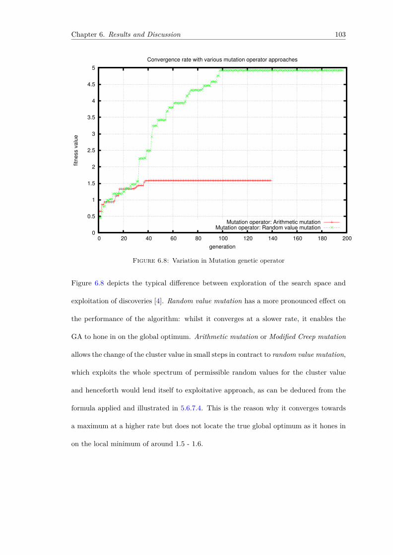
Chapter 6. Results and Discussion 103
0
0.5
1
1.5
2
2.5
3
3.5
4
4.5
5
0 20 40 60 80 100 120 140 160 180 200
fitn
ess v
alu
e
generation
Convergence rate with various mutation operator approaches
Mutation operator: Arithmetic mutationMutation operator: Random value mutation
Figure 6.8: Variation in Mutation genetic operator
Figure 6.8 depicts the typical difference between exploration of the search space and
exploitation of discoveries [4]. Random value mutation has a more pronounced effect on
the performance of the algorithm: whilst it converges at a slower rate, it enables the
GA to hone in on the global optimum. Arithmetic mutation or Modified Creep mutation
allows the change of the cluster value in small steps in contract to random value mutation,
which exploits the whole spectrum of permissible random values for the cluster value
and henceforth would lend itself to exploitative approach, as can be deduced from the
formula applied and illustrated in 5.6.7.4. This is the reason why it converges towards
a maximum at a higher rate but does not locate the true global optimum as it hones in
on the local minimum of around 1.5 - 1.6.
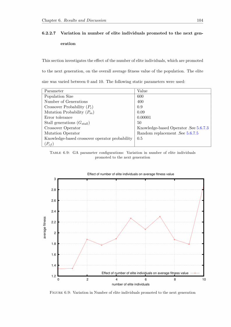
Chapter 6. Results and Discussion 104
6.2.2.7 Variation in number of elite individuals promoted to the next gen-
eration
This section investigates the effect of the number of elite individuals, which are promoted
to the next generation, on the overall average fitness value of the population. The elite
size was varied between 0 and 10. The following static parameters were used:
Parameter ValuePopulation Size 600Number of Generations 400Crossover Probability (Pc) 0.9Mutation Probability (Pm) 0.09Error tolerance 0.00001Stall generations (Gstall) 50Crossover Operator Knowledge-based Operator .See 5.6.7.3Mutation Operator Random replacement .See 5.6.7.5Knowledge-based crossover operator probability(Pcf )
0.5
Table 6.9: GA parameter configurations: Variation in number of elite individualspromoted to the next generation
1.2
1.4
1.6
1.8
2
2.2
2.4
2.6
2.8
3
0 2 4 6 8 10
ave
rag
e f
itn
ess
number of elite individuals
Effect of number of elite individuals on average fitness value
Effect of number of elite individuals on average fitness value
Figure 6.9: Variation in Number of elite individuals promoted to the next generation

Chapter 6. Results and Discussion 105
Figure 6.9 depicts, with the exception a couple of anomalies, the expected behaviour
that, if I allow for the increase of the number of the fittest individuals that are promoted
to the next generation, the average fitness will increase due to the increase in probability
that the fittest individuals will exchange genetic information. Also, the higher the
number of elite individuals, the more pronounced the effect of the fitter individual’s
fitness on the average fitness of the population.
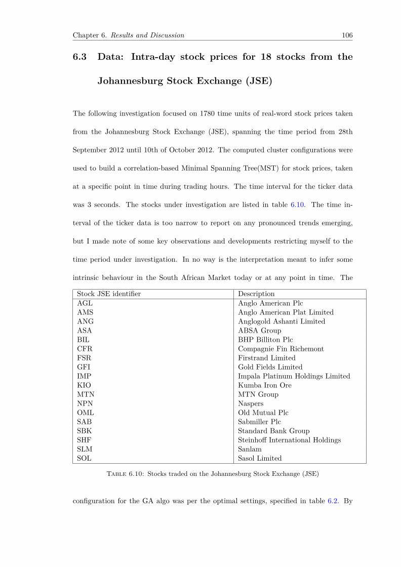
Chapter 6. Results and Discussion 106
6.3 Data: Intra-day stock prices for 18 stocks from the
Johannesburg Stock Exchange (JSE)
The following investigation focused on 1780 time units of real-word stock prices taken
from the Johannesburg Stock Exchange (JSE), spanning the time period from 28th
September 2012 until 10th of October 2012. The computed cluster configurations were
used to build a correlation-based Minimal Spanning Tree(MST) for stock prices, taken
at a specific point in time during trading hours. The time interval for the ticker data
was 3 seconds. The stocks under investigation are listed in table 6.10. The time in-
terval of the ticker data is too narrow to report on any pronounced trends emerging,
but I made note of some key observations and developments restricting myself to the
time period under investigation. In no way is the interpretation meant to infer some
intrinsic behaviour in the South African Market today or at any point in time. The
Stock JSE identifier DescriptionAGL Anglo American PlcAMS Anglo American Plat LimitedANG Anglogold Ashanti LimitedASA ABSA GroupBIL BHP Billiton PlcCFR Compagnie Fin RichemontFSR Firstrand LimitedGFI Gold Fields LimitedIMP Impala Platinum Holdings LimitedKIO Kumba Iron OreMTN MTN GroupNPN NaspersOML Old Mutual PlcSAB Sabmiller PlcSBK Standard Bank GroupSHF Steinhoff International HoldingsSLM SanlamSOL Sasol Limited
Table 6.10: Stocks traded on the Johannesburg Stock Exchange (JSE)
configuration for the GA algo was per the optimal settings, specified in table 6.2. By
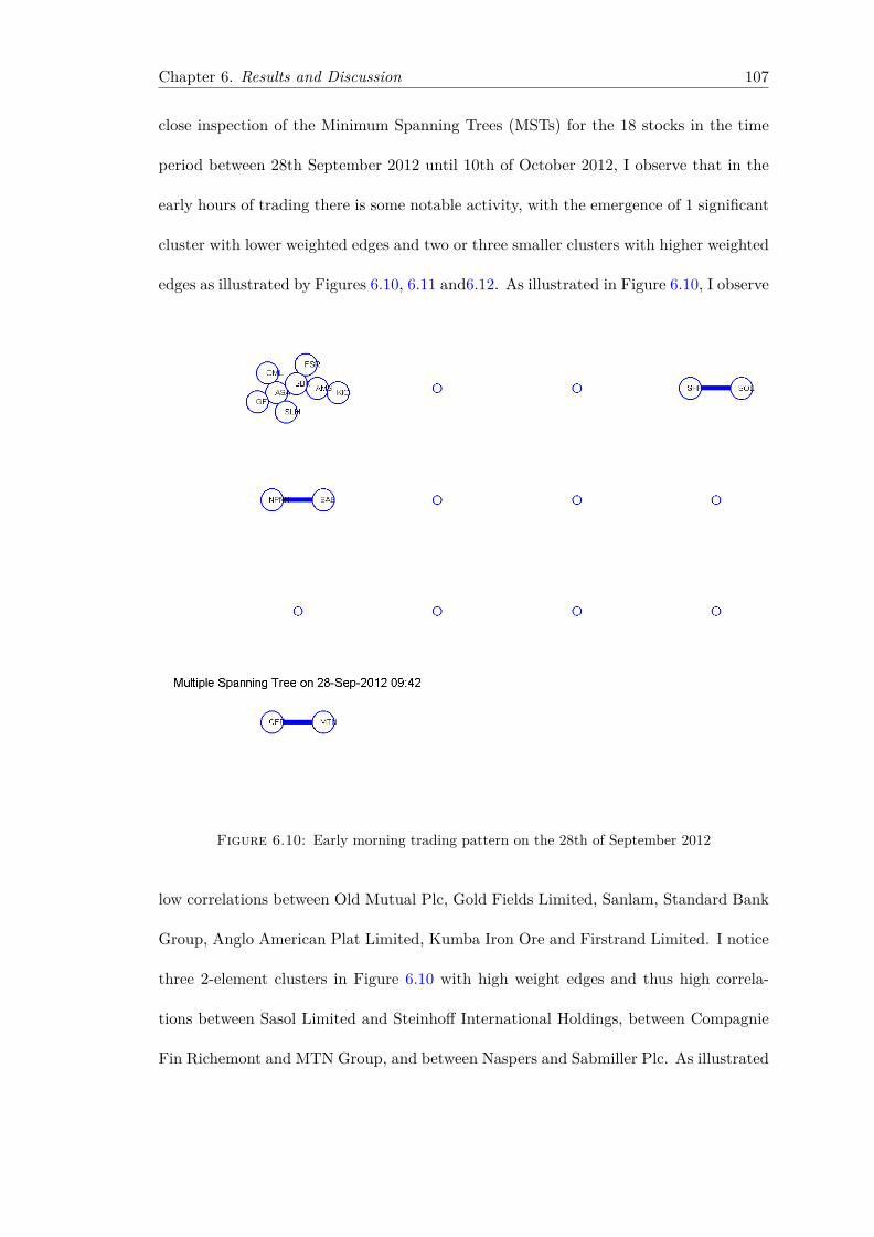
Chapter 6. Results and Discussion 107
close inspection of the Minimum Spanning Trees (MSTs) for the 18 stocks in the time
period between 28th September 2012 until 10th of October 2012, I observe that in the
early hours of trading there is some notable activity, with the emergence of 1 significant
cluster with lower weighted edges and two or three smaller clusters with higher weighted
edges as illustrated by Figures 6.10, 6.11 and6.12. As illustrated in Figure 6.10, I observe
Figure 6.10: Early morning trading pattern on the 28th of September 2012
low correlations between Old Mutual Plc, Gold Fields Limited, Sanlam, Standard Bank
Group, Anglo American Plat Limited, Kumba Iron Ore and Firstrand Limited. I notice
three 2-element clusters in Figure 6.10 with high weight edges and thus high correla-
tions between Sasol Limited and Steinhoff International Holdings, between Compagnie
Fin Richemont and MTN Group, and between Naspers and Sabmiller Plc. As illustrated
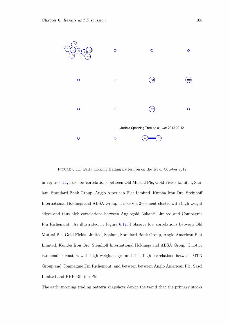
Chapter 6. Results and Discussion 108
Figure 6.11: Early morning trading pattern on on the 1st of October 2012
in Figure 6.11, I see low correlations between Old Mutual Plc, Gold Fields Limited, San-
lam, Standard Bank Group, Anglo American Plat Limited, Kumba Iron Ore, Steinhoff
International Holdings and ABSA Group. I notice a 2-element cluster with high weight
edges and thus high correlations between Anglogold Ashanti Limited and Compagnie
Fin Richemont. As illustrated in Figure 6.12, I observe low correlations between Old
Mutual Plc, Gold Fields Limited, Sanlam, Standard Bank Group, Anglo American Plat
Limited, Kumba Iron Ore, Steinhoff International Holdings and ABSA Group. I notice
two smaller clusters with high weight edges and thus high correlations between MTN
Group and Compagnie Fin Richemont, and between between Anglo American Plc, Sasol
Limited and BHP Billiton Plc
The early morning trading pattern snapshots depict the trend that the primary stocks
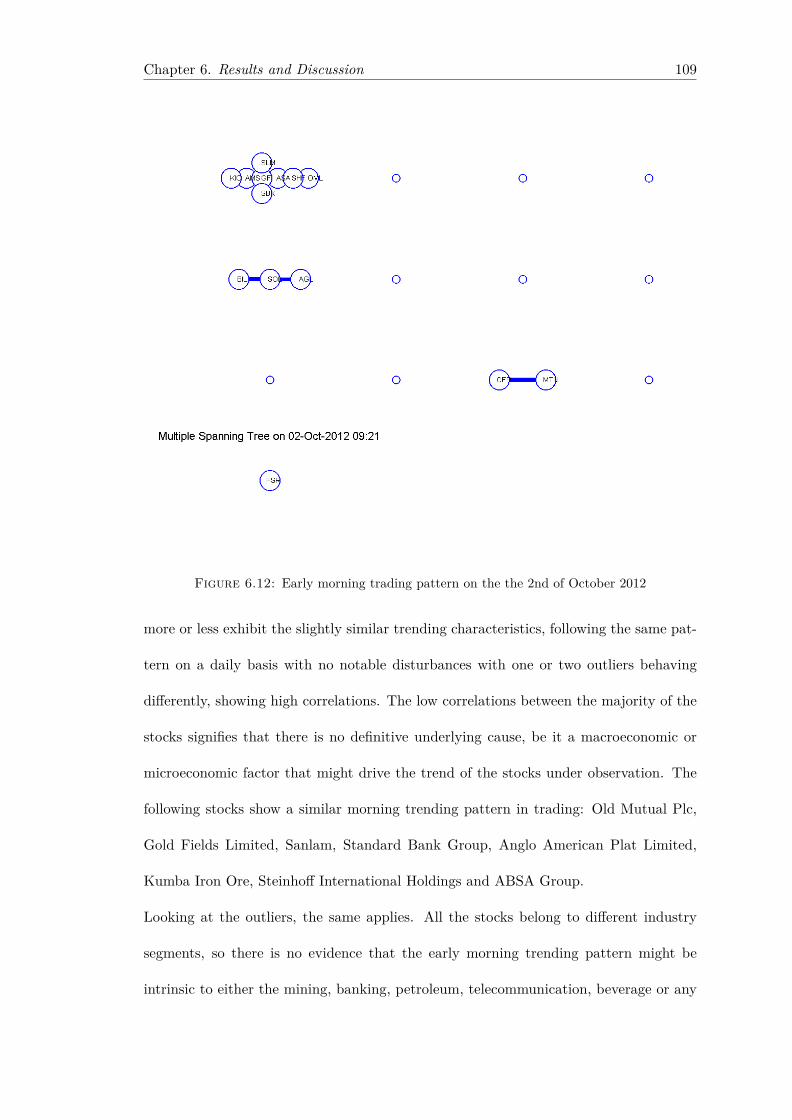
Chapter 6. Results and Discussion 109
Figure 6.12: Early morning trading pattern on the the 2nd of October 2012
more or less exhibit the slightly similar trending characteristics, following the same pat-
tern on a daily basis with no notable disturbances with one or two outliers behaving
differently, showing high correlations. The low correlations between the majority of the
stocks signifies that there is no definitive underlying cause, be it a macroeconomic or
microeconomic factor that might drive the trend of the stocks under observation. The
following stocks show a similar morning trending pattern in trading: Old Mutual Plc,
Gold Fields Limited, Sanlam, Standard Bank Group, Anglo American Plat Limited,
Kumba Iron Ore, Steinhoff International Holdings and ABSA Group.
Looking at the outliers, the same applies. All the stocks belong to different industry
segments, so there is no evidence that the early morning trending pattern might be
intrinsic to either the mining, banking, petroleum, telecommunication, beverage or any
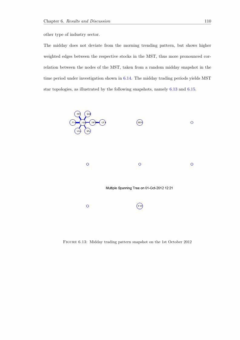
Chapter 6. Results and Discussion 110
other type of industry sector.
The midday does not deviate from the morning trending pattern, but shows higher
weighted edges between the respective stocks in the MST, thus more pronounced cor-
relation between the nodes of the MST, taken from a random midday snapshot in the
time period under investigation shown in 6.14. The midday trading periods yields MST
star topologies, as illustrated by the following snapshots, namely 6.13 and 6.15.
Figure 6.13: Midday trading pattern snapshot on the 1st October 2012
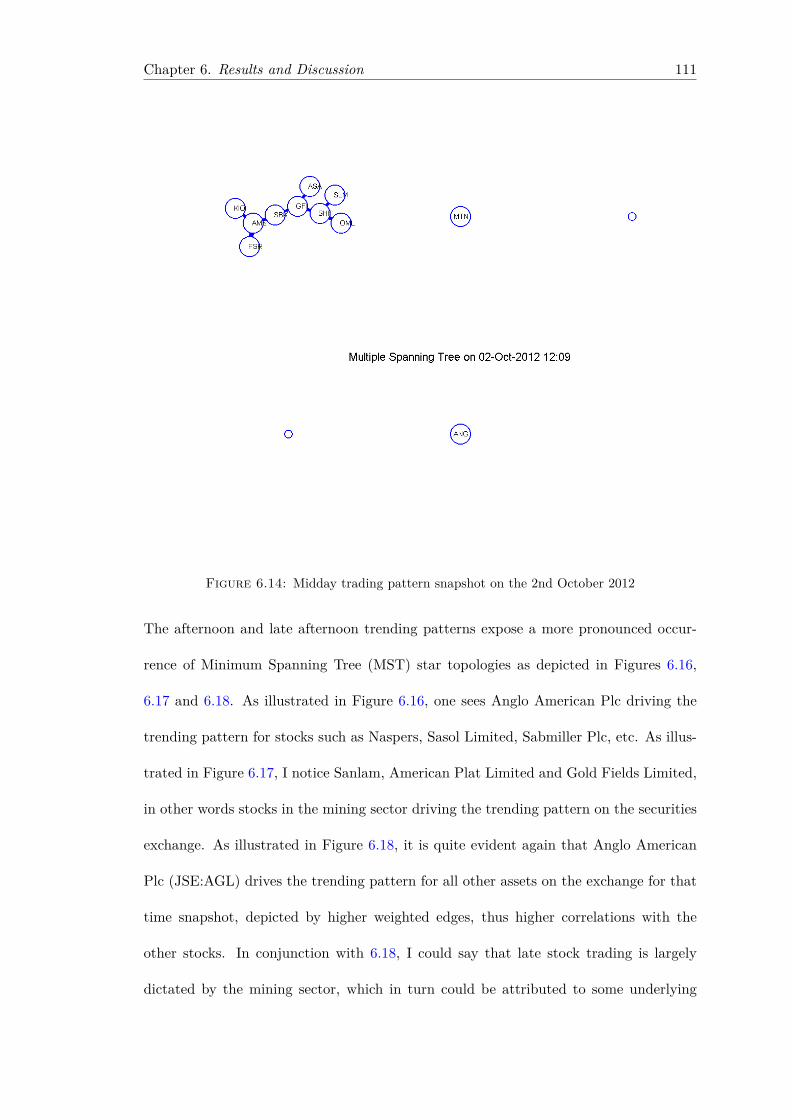
Chapter 6. Results and Discussion 111
Figure 6.14: Midday trading pattern snapshot on the 2nd October 2012
The afternoon and late afternoon trending patterns expose a more pronounced occur-
rence of Minimum Spanning Tree (MST) star topologies as depicted in Figures 6.16,
6.17 and 6.18. As illustrated in Figure 6.16, one sees Anglo American Plc driving the
trending pattern for stocks such as Naspers, Sasol Limited, Sabmiller Plc, etc. As illus-
trated in Figure 6.17, I notice Sanlam, American Plat Limited and Gold Fields Limited,
in other words stocks in the mining sector driving the trending pattern on the securities
exchange. As illustrated in Figure 6.18, it is quite evident again that Anglo American
Plc (JSE:AGL) drives the trending pattern for all other assets on the exchange for that
time snapshot, depicted by higher weighted edges, thus higher correlations with the
other stocks. In conjunction with 6.18, I could say that late stock trading is largely
dictated by the mining sector, which in turn could be attributed to some underlying
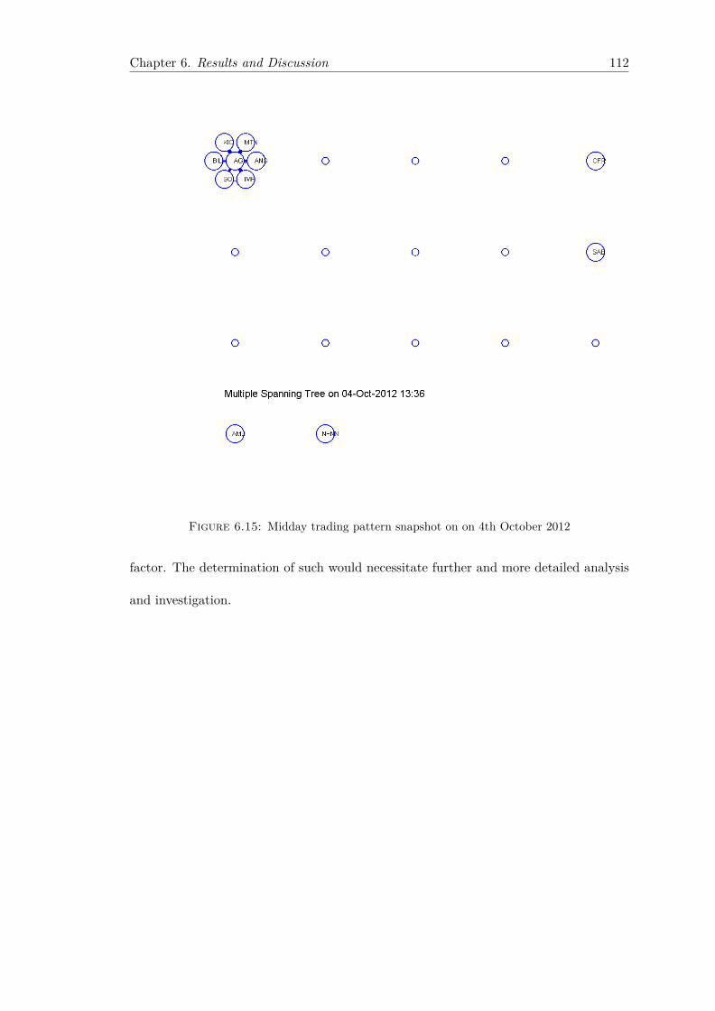
Chapter 6. Results and Discussion 112
Figure 6.15: Midday trading pattern snapshot on on 4th October 2012
factor. The determination of such would necessitate further and more detailed analysis
and investigation.
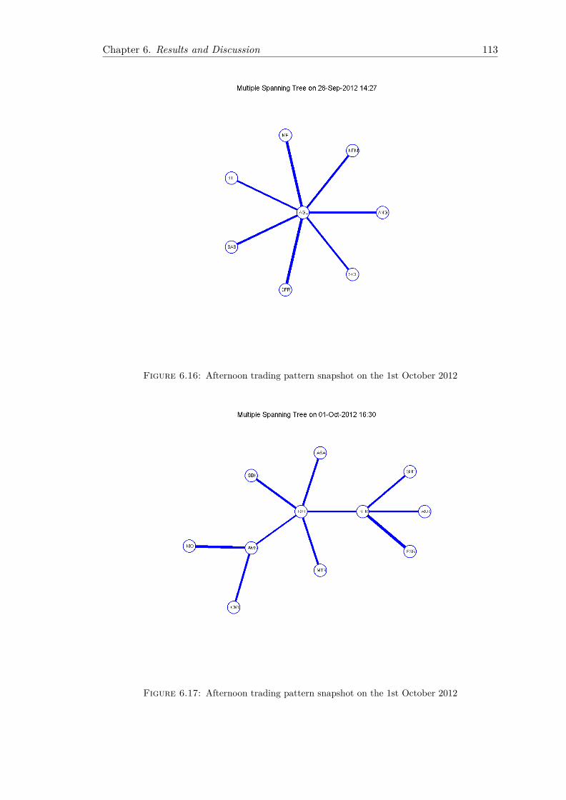
Chapter 6. Results and Discussion 113
Figure 6.16: Afternoon trading pattern snapshot on the 1st October 2012
Figure 6.17: Afternoon trading pattern snapshot on the 1st October 2012
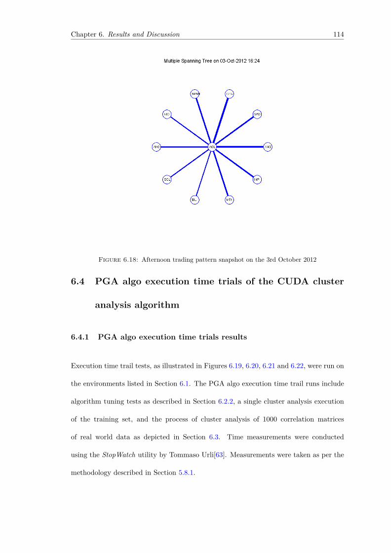
Chapter 6. Results and Discussion 114
Figure 6.18: Afternoon trading pattern snapshot on the 3rd October 2012
6.4 PGA algo execution time trials of the CUDA cluster
analysis algorithm
6.4.1 PGA algo execution time trials results
Execution time trail tests, as illustrated in Figures 6.19, 6.20, 6.21 and 6.22, were run on
the environments listed in Section 6.1. The PGA algo execution time trail runs include
algorithm tuning tests as described in Section 6.2.2, a single cluster analysis execution
of the training set, and the process of cluster analysis of 1000 correlation matrices
of real world data as depicted in Section 6.3. Time measurements were conducted
using the StopWatch utility by Tommaso Urli[63]. Measurements were taken as per the
methodology described in Section 5.8.1.
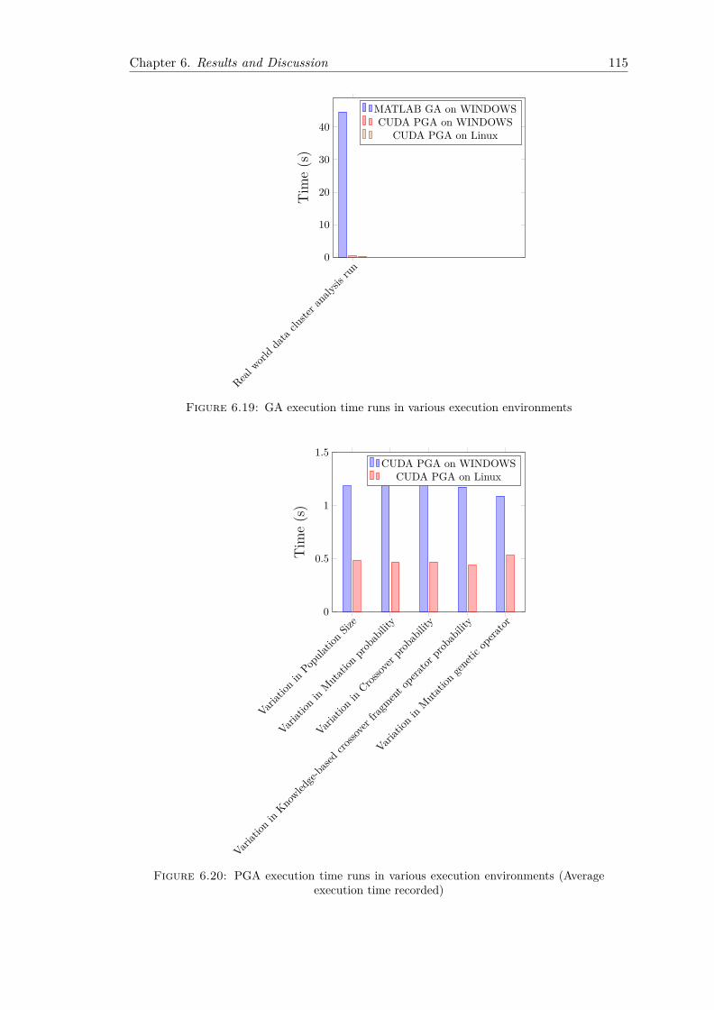
Chapter 6. Results and Discussion 115
Realworl
d data
cluste
r analy
sisrun
0
10
20
30
40
Tim
e(s
)
MATLAB GA on WINDOWSCUDA PGA on WINDOWS
CUDA PGA on Linux
Figure 6.19: GA execution time runs in various execution environments
Variati
onin
Popula
tion Siz
e
Variati
onin
Mutatio
n proba
bility
Variati
onin
Crossov
erpro
babil
ity
Variati
onin
Knowled
ge-ba
sedcro
ssover
fragm
entop
erator
proba
bility
Variati
onin
Mutatio
n geneti
c opera
tor0
0.5
1
1.5
Tim
e(s
)
CUDA PGA on WINDOWSCUDA PGA on Linux
Figure 6.20: PGA execution time runs in various execution environments (Averageexecution time recorded)
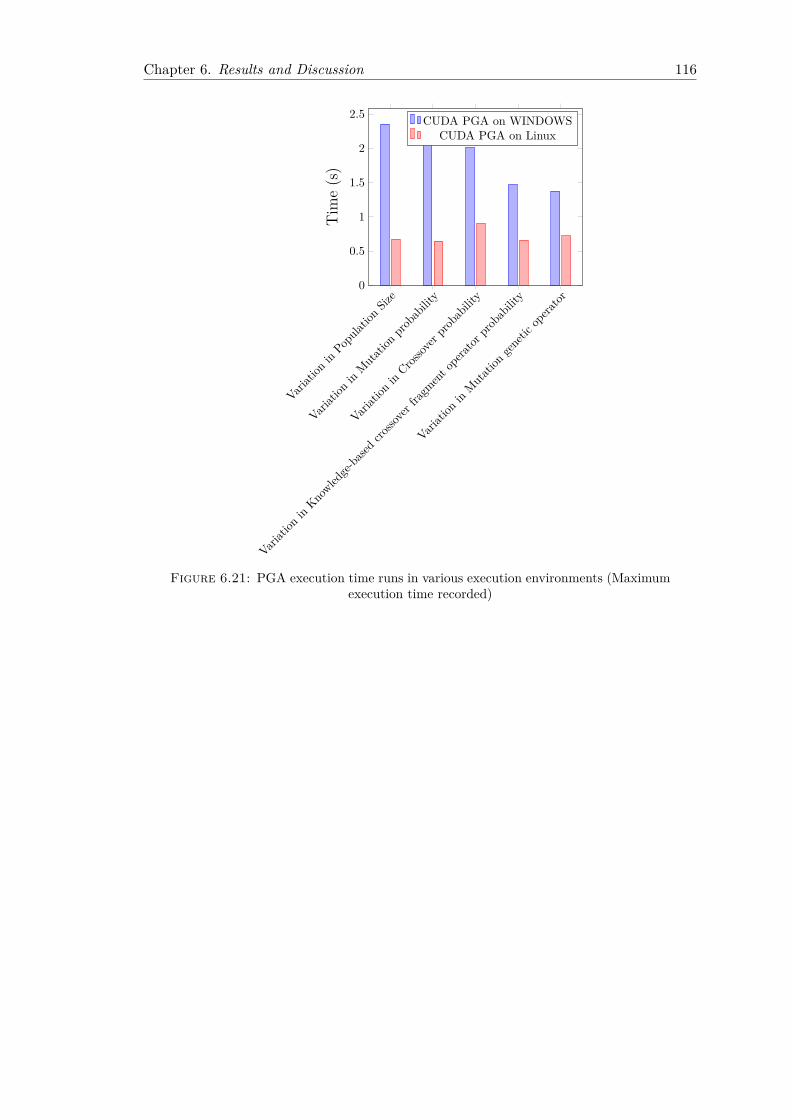
Chapter 6. Results and Discussion 116
Variati
onin
Popula
tion Siz
e
Variati
onin
Mutatio
n proba
bility
Variati
onin
Crossov
erpro
babil
ity
Variati
onin
Knowled
ge-ba
sedcro
ssover
fragm
entop
erator
proba
bility
Variati
onin
Mutatio
n geneti
c opera
tor0
0.5
1
1.5
2
2.5
Tim
e(s
)
CUDA PGA on WINDOWSCUDA PGA on Linux
Figure 6.21: PGA execution time runs in various execution environments (Maximumexecution time recorded)
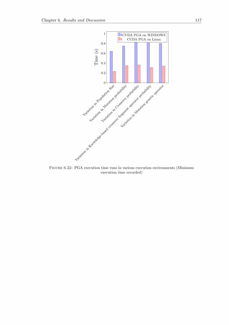
Chapter 6. Results and Discussion 117
Variati
onin
Popula
tion Siz
e
Variati
onin
Mutatio
n proba
bility
Variati
onin
Crossov
erpro
babil
ity
Variati
onin
Knowled
ge-ba
sedcro
ssover
fragm
entop
erator
proba
bility
Variati
onin
Mutatio
n geneti
c opera
tor0
0.2
0.4
0.6
0.8
1
Tim
e(s
)
CUDA PGA on WINDOWSCUDA PGA on Linux
Figure 6.22: PGA execution time runs in various execution environments (Minimumexecution time recorded)
Chapter 6. Results and Discussion 118
6.4.2 Analysis of GA algo execution time trials
The results show a clear picture of the efficiency of the CUDA PGA implementation.
The performance improvement in the case of the training set cluster analysis run is in the
region of 13 000% on the Linux, 6500% on the Windows. This can be attributed to the
utilisation of a parallel computation platform, a novel genetic operator and the extensive
and comprehensive algorithm tuning techniques employed. Similar performance gains
are also observed in the real world data code execution time runs, namely that the
CUDA PGA executes at around 100 times faster than the serial MATLAB GA algorithm.
Shifting the focus to the various algorithm tuning runs, I noticed that, on average, there
is a very notable performance improvement between the LINUX and the WINDOWS
platform. The same compilation options were utilised on both platforms, but the code
optimised for the Linux platform. This might explain the discrepancy in execution times
between LINUX and the WINDOWS environment. In order to make a more substantial
assessment, I would have to profile the algorithm on both platforms and investigate the
causes for the discrepancies; but this is beyond the scope of this research.
Chapter 7
Conclusions and future prospects
7.1 Conclusions
The range of investigations that were undertaken show that the Giada and Marsili likeli-
hood function[11], inspired by the Noh model, is a viable approach for isolating residual
clusters in data-sets. Its key advantages, in comparison to conventional clustering meth-
ods, are that it is unsupervised and that the interpretation of results is transparent in
terms of the model.
Two evolutionary search heuristics were reviewed, namely the Master-slave Parallel Ge-
netic Algorithm and the Multipe-deme Parallel Genetic Algorithm. The implementation
of the Master-slave PGA showed that the efficiency depends on various parameter set-
tings and that fine-tuning such an algorithm is not easy. The research shows that the
PGA efficiency is largely dependant on the size of the population, a statement which is
also supported by literature[6], but entails a higher computational cost and utilisation
of memory resources. The increased crossover probability increases the chromosome
gene recombination probability and thus, on average, enables the PGA to generate fitter
119
Chapter 7. Conclusion and future prospects 120
individuals. The same applies to the mutation probability. A novel knowledge based
crossover operator was introduced. The results show that it outperforms traditional
crossover operators, such as Single-point crossover and Two-point crossover genetic op-
erators as the PGA achieves higher convergence rates and creates successive populations
with higher average fitness values. The type of mutation operator utilised has a pro-
nounced effect on the algorithm’s efficiency to isolate the optimal solution in the search
space, whereas other parameter settings primarily impact the convergence rate. The
Arithmetic mutation operator allows the PGA to create offspring with optimal fitness
values. The final test run investigated the effect of the number of elite individuals, that
are promoted to the next generation on the average fitness of the successive generation.
I can conclude, that, the higher the number of elite individuals that are promoted, the
higher the average fitness value of the successive generation and thus the higher the
quality of offspring created. According to the time trial results, the CUDA PGA imple-
mentation runs 100-130 times faster than the serial GA implementation in MATLAB,
which is the true litmus test of the success of the research undertaken. It illustrates that
the application of the Master-slave Parallel Genetic Algorithm (PGA) framework for
unsupervised cluster analysis on the CUDA platform, using the Giada and Marsili log-
likelihood function as the fitness function, is a novel and promising new cluster analysis
approach.
7.2 Future prospects
The current configuration of the Master-slave algorithm only allows for a minimal util-
isation of the computational platform, using a fraction of the memory and processing
capability due to the small size of the data-sets utilised. In theory, I could improve
Chapter 7. Conclusion and future prospects 121
on the Master-slave algorithm by fully exploiting the extent of resources that the GPU
provides and as such, fully utilise the whole grid of thread blocks and run multiple clus-
tering analysis processes in tandem. This would boost the efficiency of the Master-slave
PGA and result in a novel hybrid Master-slave PGA for cluster analysis, where huge
low-latency data feeds could be harvested for cluster characteristics in a fraction of the
time it would take other algorithms to derive similar results.
Future prospects would include the proper implementation, testing and research of a
Multiple-deme PGA on the GPGPU platform. Research, presented in Section 3.2.3,
shows that the Multiple-deme approach scheme shows the most promise in terms of
computational performance, and that it warrants further investigation.
Bibliography
[1] Marek Rucinski, Dario Izzo, and Francesco Biscani. On the impact of the migration
topology on the island model. CoRR, abs/1004.4541, 2010.
[2] R.B. Litterman and Goldman Sachs Asset Management. Quantitative Resources
Group. Modern Investment Management: An Equilibrium Approach. Wiley Finance
Series. John Wiley, 2003. ISBN 9780471124108. URL http://books.google.co.
za/books?id=k8Jyhasdu98C.
[3] D. Barbara. An introduction to cluster analysis for data mining. 2000.
[4] D.A. Coley. An Introduction to Genetic Algorithms for Scientists and Engineers.
World Scientific, 1999. ISBN 9789810236021. URL http://books.google.co.za/
books?id=-D568prVv0QC.
[5] Lawrence Davis. Handbook of Genetic Algorithms. Van Nostrand Reinhold, 1991.
[6] S.N. Sivanandam and S.N. Deepa. Introduction to Genetic Algorithms. Springer,
2010. ISBN 9783642092244.
[7] NVIDIA. NVIDIA CUDA C Programming Guide. NVIDIA Corporation, 2011.
[8] NVIDIA. CUDA DYNAMIC PARALLELISM PROGRAMMING GUIDE.
NVIDIA Corporation, 2012.
122
Bibliography 123
[9] Petr Pospichal, Jiri Jaros, and Josef Schwarz. Parallel genetic algorithm on the
CUDA architecture. In Proceedings of the 2010 international conference on Ap-
plications of Evolutionary Computation - Volume Part I, EvoApplicatons’10, pages
442–451, Berlin, Heidelberg, 2010. Springer-Verlag. ISBN 3-642-12238-8, 978-3-642-
12238-5.
[10] Sifa Zhang and Zhenming He. Implementation of parallel genetic algorithm based
on cuda. In Proceedings of the 4th International Symposium on Advances in Compu-
tation and Intelligence, ISICA ’09, pages 24–30, Berlin, Heidelberg, 2009. Springer-
Verlag. ISBN 978-3-642-04842-5.
[11] Lorenzo Giada and Matteo Marsili. Algorithms of maximum likelihood
data clustering with applications. Physica A: Statistical Mechanics and its
Applications, 315(3âĂŞ4):650 – 664, 2002. ISSN 0378-4371. doi: 10.
1016/S0378-4371(02)00974-3. URL http://www.sciencedirect.com/science/
article/pii/S0378437102009743.
[12] B. Mbambiso. Dissecting the south african equity markets into sectors and states.
Master’s thesis, Faculty of Science, University of Cape Town, February 2009.
[13] J.D Noh. Phys. Rev. E, 61, 2000.
[14] T. Gebbie. (Private communication) Unparallized GA implementation of the like-
lihood function implemented in MATLAB, 2012.
[15] Erik Mooi and Marko Sarstedt. A Concise Guide to Market Research. Springer
Berlin Heidelberg, 2011. ISBN 978-3-642-12540-9. URL http://www-users.cs.
umn.edu/˜kumar/dmbook/.
Bibliography 124
[16] Jeff Bacidore, Kathryn Berkow, Ben Polidore, and Saraiya Nigam. Cluster Analysis
for Evaluating Trading Strategies. The Journal of Trading, 7(3), 2012. URL http:
//www.iijournals.com/doi/abs/10.3905/jot.2012.7.3.006.
[17] Newton Da Costa Jr, Jefferson Cunha, and Sergio Da Silva. Stock Selection Based
on Cluster Analysis. Economics Bulletin, 2005.
[18] Lorenzo Giada and Matteo Marsili. Data clustering and noise undressing of corre-
lation matrices. Phys. Rev. E, 63:061101, May 2001. doi: 10.1103/PhysRevE.63.
061101. URL http://link.aps.org/doi/10.1103/PhysRevE.63.061101.
[19] S. Kirkpatrick, C. D. Gelatt, and M. P. Vecchi. Optimization by simulated anneal-
ing. Science, 220(4598):671–680, 1983. doi: 10.1126/science.220.4598.671. URL
http://www.sciencemag.org/content/220/4598/671.abstract.
[20] Cowgill Marc C., Harvey Robert J., and Watson Layne T. A genetic algorithm
approach to cluster analysis. Technical report, Virginia Polytechnic Institute &
State University, Blacksburg, VA, USA, 1998.
[21] Turku Centre For, Juha KivijÃďrvi, Juha Kivijrvi, Joonas Lehtinen, Joonas Lehti-
nen, Olli Nevalainen, and Olli Nevalainen. A parallel genetic algorithm for cluster-
ing, 2002.
[22] Jian-Hui Jiang, Ji-Hong Wang, Xia Chu, and Ru-Qin Yu. Clustering data using
a modified integer genetic algorithm (iga). Analytica Chimica Acta, 354(1âĂŞ3):
263 – 274, 1997. ISSN 0003-2670. doi: 10.1016/S0003-2670(97)00462-5. URL
http://www.sciencedirect.com/science/article/pii/S0003267097004625.
[23] L.E. AgustĜn-Blas, S. Salcedo-Sanz, S. JimÃľnez-FernÃąndez, L. Carro-Calvo,
J. Del Ser, and J.A. Portilla-Figueras. A new grouping genetic algorithm for clus-
tering problems. Expert Systems with Applications, 39(10):9695 – 9703, 2012. ISSN
Bibliography 125
0957-4174. doi: 10.1016/j.eswa.2012.02.149. URL http://www.sciencedirect.
com/science/article/pii/S0957417412004125.
[24] Ujjwal Maulik, Sanghamitra Bandyopadhyay, and Sanghamitra B. Genetic
algorithm-based clustering technique. Pattern Recognition, 33:1455–1465, 2000.
[25] Abbas Mahmoudabadi and Reza Tavakkoli-Moghaddam. The use of a genetic
algorithm for clustering the weighing station performance in transportation - a
case study. Expert Syst. Appl., 38(9):11744–11750, 2011. URL http://dblp.
uni-trier.de/db/journals/eswa/eswa38.html#MahmoudabadiT11.
[26] A. O. Adewumi and M. M. Ali. A multi-level genetic algorithm for a multi-stage
space allocation problem. Math. Comput. Model., 51(1-2):109–126, January 2010.
ISSN 0895-7177. doi: 10.1016/j.mcm.2009.09.004. URL http://dx.doi.org/10.
1016/j.mcm.2009.09.004.
[27] Mohamad M. Tawfick, Hazem M. Abbas, and Hussein I. Shahein. An integer-
coded evolutionary approach for mixture maximum likelihood clustering. Pat-
tern Recognition Letters, 29(4):515 – 524, 2008. ISSN 0167-8655. doi: 10.1016/
j.patrec.2007.11.003. URL http://www.sciencedirect.com/science/article/
pii/S0167865507003625.
[28] Cezary Z. Janikow and Zbigniew Michalewicz. An experimental comparison of
binary and floating point representations in genetic algorithms. In ICGA, pages
31–36, 1991.
[29] Gaowei Yan, Gang Xie, Zehua Chen, and Keming Xie. Knowledge-based genetic
algorithms. In Guoyin Wang, Tianrui Li, JerzyW. Grzymala-Busse, Duoqian Miao,
Andrzej Skowron, and Yiyu Yao, editors, Rough Sets and Knowledge Technology,
volume 5009 of Lecture Notes in Computer Science, pages 148–155. Springer Berlin
Bibliography 126
Heidelberg, 2008. ISBN 978-3-540-79720-3. doi: 10.1007/978-3-540-79721-0 24.
URL http://dx.doi.org/10.1007/978-3-540-79721-0_24.
[30] Erick CantÞ-Paz and David E. Goldberg. Efficient parallel genetic al-
gorithms: theory and practice. Computer Methods in Applied Mechanics
and Engineering, 186(2âĂŞ4):221 – 238, 2000. ISSN 0045-7825. doi: 10.
1016/S0045-7825(99)00385-0. URL http://www.sciencedirect.com/science/
article/pii/S0045782599003850.
[31] Erick Cantu-Paz. Topologies, migration rates, and multi-population parallel ge-
netic algorithms. In Wolfgang Banzhaf, Jason Daida, Agoston E. Eiben, Max H.
Garzon, Vasant Honavar, Mark Jakiela, and Robert E. Smith, editors, Proceedings
of the Genetic and Evolutionary Computation Conference, volume 1, pages 91–98,
Orlando, Florida, USA, 13-17 July 1999. Morgan Kaufmann. ISBN 1-55860-611-4.
URL http://dangermouse.brynmawr.edu/ec/gecco99-topologies.pdf.
[32] Marek Rucinski, Dario Izzo, and Francesco Biscani. The generalized island model.
Parallel Architectures & Bioinspired Algorithms, pages 151–169, 2012.
[33] M. Flynn. Some computer organizations and their effectiveness. Computers, IEEE
Transactions on, C-21(9):948–960, Sept 1972. ISSN 0018-9340. doi: 10.1109/TC.
1972.5009071.
[34] David Culler, J.P. Singh, and Anoop Gupta. Parallel Computer Ar-
chitecture: A Hardware/Software Approach. Morgan Kaufmann, 1st
edition, 1998. ISBN 1558603433. URL http://www.amazon.com/
Parallel-Computer-Architecture-Hardware-Software/dp/1558603433. The
Morgan Kaufmann Series in Computer Architecture and Design.
Bibliography 127
[35] Barry Wilkinson and Michael Allen. Parallel programming - techniques and ap-
plications using networked workstations and parallel computers (2. ed.). Pearson
Education, 2005. ISBN 978-0-13-191865-8.
[36] Jack Dongarra, Steve W. Otto, Marc Snir, and David W. Walker. A message passing
standard for mpp and workstations. Commun. ACM, 39(7):84–90, 1996. URL
http://dblp.uni-trier.de/db/journals/cacm/cacm39.html#DongarraOSW96.
[37] Rudolf Eigenmann and Michael Voss, editors. OpenMP Shared Memory Parallel
Programming, International Workshop on OpenMP Applications and Tools, WOM-
PAT 2001, West Lafayette, IN, USA, July 30-31, 2001 Proceedings, volume 2104
of Lecture Notes in Computer Science, 2001. Springer. ISBN 3-540-42346-X. URL
http://dblp.uni-trier.de/db/conf/wompat/wompat2001.html.
[38] C. Leopold. Parallel and Distributed Computing: A Survey of Models,
Paradigms and Approaches. A Wiley-Interscience publication. Wiley, 2001. ISBN
9780471358312. URL http://books.google.co.za/books?id=J1MZAQAAIAAJ.
[39] Tabitha L. James, Reza Barkhi, and John D. Johnson. Platform impact on per-
formance of parallel genetic algorithms: Design and implementation considera-
tions. Engineering Applications of Artificial Intelligence, 19(8):843 – 856, 2006.
ISSN 0952-1976. doi: http://dx.doi.org/10.1016/j.engappai.2006.02.004. URL
http://www.sciencedirect.com/science/article/pii/S0952197606000558.
[40] Julien C. Thibault and Inanc Senocak. Accelerating incompressible flow com-
putations with a Pthreads-CUDA implementation on small-footprint multi-
GPU platforms. J. Supercomput., 59(2):693–719, February 2012. ISSN 0920-
8542. doi: 10.1007/s11227-010-0468-1. URL http://dx.doi.org/10.1007/
s11227-010-0468-1.
Bibliography 128
[41] NVIDIA. CUDA C BEST PRACTICES GUIDE. NVIDIA Corporation, 2012.
[42] A.R. Brodtkorb and et al. Graphics processing unit (GPU) programming strategies
and trends in GPU computing. J. Parallel Distrib. Comput., 73(1):4–13, 2013. ISSN
0743-7315. doi: 10.1016/j.jpdc.2012.04.003. URL http://dx.doi.org/10.1016/
j.jpdc.2012.04.003.
[43] Shucai Xiao and Wu chun Feng. Inter-block GPU communication via fast bar-
rier synchronization. In IPDPS, pages 1–12. IEEE, 2010. URL http://dblp.
uni-trier.de/db/conf/ipps/ipdps2010.html#XiaoF10.
[44] Donald E. Knuth. Structured programming with GOTO statements. Computing
Surveys, 6:261–301, 1974.
[45] Hiroyasu Tomoyuki, Yamanaka Ryosuke, Yoshimi Masato, and Miki Mitsunori.
Garop: Genetic algorithm framework for running on parallel environments. IPSJ
SIG Notes, 2012(5):1–6, jul 2012. ISSN 09196072. URL http://ci.nii.ac.jp/
naid/110009421221/en/.
[46] R. N. Mantegna. Hierarchical structure in financial markets. European Physical
Journal B, 11:193–197, 1999.
[47] Giovanni Bonanno, Guido Caldarelli, Fabrizio Lillo, and Rosario N. Mantegna.
Topology of correlation-based minimal spanning trees in real and model markets.
Physical Review E (Statistical, Nonlinear, and Soft Matter Physics), 68(4):046130+,
2003. URL http://dx.doi.org/10.1103/physreve.68.046130.
[48] Tim Gebbie and Diane Wilcox. (Private Communication) MATLAB data pre-
processing libraries and data, 2012.
Bibliography 129
[49] T. Gebbie. (Private Communication) MATLAB Minimal Spanning Tree code li-
braries for the generation of tree and the animation thereof., 2012.
[50] Paris Avgeriou and Uwe Zdun. Architectural patterns revisited âĂŞ a pattern
language. In In 10th European Conference on Pattern Languages of Programs (Eu-
roPlop 2005), Irsee, pages 1–39, 2005.
[51] NVIDIA. CUDA C BEST PRACTICES GUIDE. NVIDIA Corporation, 2012.
[52] Michal Czapinski and Stuart Barnes. Tabu Search with two approaches to parallel
flowshop evaluation on CUDA platform. J. Parallel Distrib. Comput., 71(6):802–
811, 2011. ISSN 0743-7315.
[53] Denis Robilliard, Virginie Marion-Poty, and Cyril Fonlupt. Genetic programming
on graphics processing units. Genetic Programming and Evolvable Machines, 10(4):
447–471, December 2009. ISSN 1389-2576. doi: 10.1007/s10710-009-9092-3. URL
http://dx.doi.org/10.1007/s10710-009-9092-3.
[54] W. B. Langdon. A fast high quality pseudo random number generator for nVidia
CUDA. In Proceedings of the 11th Annual Conference Companion on Genetic and
Evolutionary Computation Conference: Late Breaking Papers, GECCO ’09, pages
2511–2514, New York, NY, USA, 2009. ACM. ISBN 978-1-60558-505-5. doi: 10.
1145/1570256.1570353. URL http://doi.acm.org/10.1145/1570256.1570353.
[55] Sain-Zee Ueng, Melvin Lathara, Sara S. Baghsorkhi, and Wen-Mei W. Hwu. Cuda-
lite: Reducing gpu programming complexity. In Jose Nelson Amaral, editor, Lan-
guages and Compilers for Parallel Computing, pages 1–15. Springer-Verlag, Berlin,
Heidelberg, 2008. ISBN 978-3-540-89739-2.
Bibliography 130
[56] Dehao Chen, Wenguang Chen, and Weimin Zheng. CUDA-Zero: a framework
for porting shared memory GPU applications to multi-GPUs. SCIENCE CHINA
Information Sciences, 55(3):663–676, 2012.
[57] John A. Stratton, Sam S. Stone, and Wen-Mei W. Hwu. Mcuda: An efficient
implementation of cuda kernels for multi-core cpus. In Jose Nelson Amaral, editor,
Languages and Compilers for Parallel Computing, pages 16–30. Springer-Verlag,
Berlin, Heidelberg, 2008. ISBN 978-3-540-89739-2.
[58] William B. Langdon. Debugging cuda. In Proceedings of the 13th annual conference
companion on Genetic and evolutionary computation, GECCO ’11, pages 415–422,
New York, NY, USA, 2011. ACM. ISBN 978-1-4503-0690-4.
[59] NVIDIA. The CUDA Compiler Driver NVCC Manual. NVIDIA Corporation, 2011.
[60] NVIDIA. CUDA-GDB: The NVIDIA CUDA Debugger Manual. NVIDIA Corpo-
ration, 2011.
[61] NVIDIA. CUDA CURAND Guide. NVIDIA Corporation, 2012.
[62] NVIDIA. CUDA Toolkit 4.0 Thrust Quick Start Guide. NVIDIA Corporation,
2011.
[63] T. Urli. Stopwatch implementation for C++, 2010.


