
Topology-Constrained Surface Reconstruction From Cross-sections
Ming Zou∗ Michelle Holloway † Nathan Carr ‡ Tao Ju§
Washington U. in St. Louis Washington U. in St. Louis Adobe Washington U. in St. Louis
Figure 1: Non-parallel cross-section curves delineating a developing chicken heart from a CT volume (a) and the reconstructed surfacesusing the method of Lu et al. [2008] (b), method of Bermano et al. [2011] (c), and our method with genus-1 constraint without utilizing theCT volume (d). The first two surfaces contain numerous topological tunnels, while ours correctly captures the shell-like shape of the object.
Abstract
In this work we detail the first algorithm that provides topologi-cal control during surface reconstruction from an input set of pla-nar cross-sections. Our work has broad application in a numberof fields including surface modeling and biomedical image anal-ysis, where surfaces of known topology must be recovered. Givencurves on arbitrarily oriented cross-sections, our method produces amanifold interpolating surface that exactly matches a user-specifiedgenus. The key insight behind our approach is to formulate thetopological search as a divide-and-conquer optimization processwhich scores local sets of topologies and combines them to sat-isfy the global topology constraint. We further extend our methodto allow image data to guide the topological search, achieving evenbetter results than relying on the curves alone. By simultaneouslysatisfying both geometric and topological constraints, we are ableto produce accurate reconstructions with fewer input cross-sections,hence reducing the manual time needed to extract the desired shape.
CR Categories: I.3.5 [Computer Graphics]: Computational Ge-ometry and Object Modeling—Geometric algorithms, languages,and systems
Keywords: Surface reconstruction, cross-section interpolation,contour stitching, topology constraint, dynamic programming
∗e-mail:[email protected]†e-mail:[email protected]‡e-mail:[email protected]§e-mail:[email protected]
1 Introduction
The need to create surfaces depicting a 3D object from its cross-sections arises in many applications. For instance, in order to re-construct the surface of an organ captured by CT or MRI, radiolo-gists typically start by manually delineating the organ boundary onselected 2D slices of the 3D image volume. The delineated planarcurves then need to be connected to form a closed surface. Figure1 (a) shows an example stack of the delineated curves of a layer ofa developing chicken heart from a CT volume (images on the rightshow two slices through the CT volume).
In many application domains, there exists strong prior informationabout the object to be depicted. One piece of such information istopology, which describes the object’s connected components andtheir genus. For example, a biological structure usually has a knowntopology. Most structures have the topology of a sphere, whichis a single component with zero genus. Some structures have amore complicated topology. A layer of a developing chicken heartis a cylindrical shell with genus 1. Bones in our body, such asvertebrae and the hip bone, can have a higher genus. Accuratelycapturing such topology not only helps with recovering the shapeof the object but is also important for downstream applications ofthe reconstructed surface, such as shape matching, fluid dynamicssimulation, and mechanical analysis.
Much research has been done for creating surfaces from cross-sections (see a more detailed review in Section 2). While thestate-of-the-art algorithms are capable of creating watertight sur-faces from even the most complex inputs, no method to date canguarantee that their output has a predefined topology. In fact, it isquite common for these methods to create topological errors, par-ticularly when the cross-sections are not dense (see Figure 1 (b,c)).While it is possible for these methods to achieve the correct topol-ogy by providing them with more cross-sections, this will requireadditional manual labor and the data may not be available at all.
In this paper, we present a novel algorithm for reconstruction fromcross-sections that allows precise control over surface topology
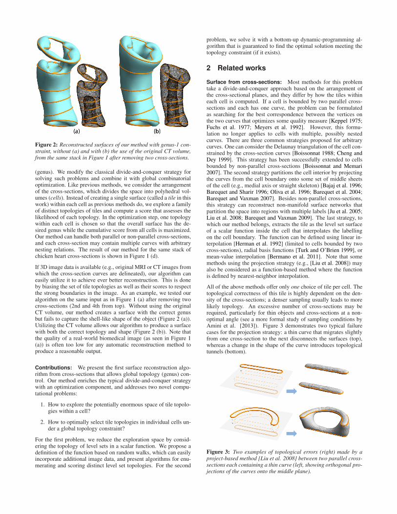
Figure 2: Reconstructed surfaces of our method with genus-1 con-straint, without (a) and with (b) the use of the original CT volume,from the same stack in Figure 1 after removing two cross-sections.
(genus). We modify the classical divide-and-conquer strategy forsolving such problems and combine it with global combinatorialoptimization. Like previous methods, we consider the arrangementof the cross-sections, which divides the space into polyhedral vol-umes (cells). Instead of creating a single surface (called a tile in thiswork) within each cell as previous methods do, we explore a familyof distinct topologies of tiles and compute a score that assesses thelikelihood of each topology. In the optimization step, one topologywithin each cell is chosen so that the overall surface has the de-sired genus while the cumulative score from all cells is maximized.Our method can handle both parallel or non-parallel cross-sections,and each cross-section may contain multiple curves with arbitrarynesting relations. The result of our method for the same stack ofchicken heart cross-sections is shown in Figure 1 (d).
If 3D image data is available (e.g., original MRI or CT images fromwhich the cross-section curves are delineated), our algorithm caneasily utilize it to achieve ever better reconstruction. This is doneby biasing the set of tile topologies as well as their scores to respectthe strong boundaries in the image. As an example, we tested ouralgorithm on the same input as in Figure 1 (a) after removing twocross-sections (2nd and 4th from top). Without using the originalCT volume, our method creates a surface with the correct genusbut fails to capture the shell-like shape of the object (Figure 2 (a)).Utilizing the CT volume allows our algorithm to produce a surfacewith both the correct topology and shape (Figure 2 (b)). Note thatthe quality of a real-world biomedical image (as seen in Figure 1(a)) is often too low for any automatic reconstruction method toproduce a reasonable output.
Contributions: We present the first surface reconstruction algo-rithm from cross-sections that allows global topology (genus) con-trol. Our method enriches the typical divide-and-conquer strategywith an optimization component, and addresses two novel compu-tational problems:
1. How to explore the potentially enormous space of tile topolo-gies within a cell?
2. How to optimally select tile topologies in individual cells un-der a global topology constraint?
For the first problem, we reduce the exploration space by consid-ering the topology of level sets in a scalar function. We propose adefinition of the function based on random walks, which can easilyincorporate additional image data, and present algorithms for enu-merating and scoring distinct level set topologies. For the second
problem, we solve it with a bottom-up dynamic-programming al-gorithm that is guaranteed to find the optimal solution meeting thetopology constraint (if it exists).
2 Related works
Surface from cross-sections: Most methods for this problemtake a divide-and-conquer approach based on the arrangement ofthe cross-sectional planes, and they differ by how the tiles withineach cell is computed. If a cell is bounded by two parallel cross-sections and each has one curve, the problem can be formulatedas searching for the best correspondence between the vertices onthe two curves that optimizes some quality measure [Keppel 1975;Fuchs et al. 1977; Meyers et al. 1992]. However, this formu-lation no longer applies to cells with multiple, possibly nestedcurves. There are three common strategies proposed for arbitrarycurves. One can consider the Delaunay triangulation of the cell con-strained by the cross-section curves [Boissonnat 1988; Cheng andDey 1999]. This strategy has been successfully extended to cellsbounded by non-parallel cross-sections [Boissonnat and Memari2007]. The second strategy partitions the cell interior by projectingthe curves from the cell boundary onto some set of middle sheetsof the cell (e.g., medial axis or straight skeleton) [Bajaj et al. 1996;Barequet and Sharir 1996; Oliva et al. 1996; Barequet et al. 2004;Barequet and Vaxman 2007]. Besides non-parallel cross-sections,this strategy can reconstruct non-manifold surface networks thatpartition the space into regions with multiple labels [Ju et al. 2005;Liu et al. 2008; Barequet and Vaxman 2009]. The last strategy, towhich our method belongs, extracts the tile as the level set surfaceof a scalar function inside the cell that interpolates the labellingon the cell boundary. The function can be defined using linear in-terpolation [Herman et al. 1992] (limited to cells bounded by twocross-sections), radial basis functions [Turk and O’Brien 1999], ormean-value interpolation [Bermano et al. 2011]. Note that somemethods using the projection strategy (e.g., [Liu et al. 2008]) mayalso be considered as a function-based method where the functionis defined by nearest-neighbor interpolation.
All of the above methods offer only one choice of tile per cell. Thetopological correctness of this tile is highly dependent on the den-sity of the cross-sections; a denser sampling usually leads to morelikely topology. An excessive number of cross-sections may berequired, particularly for thin objects and cross-sections at a non-optimal angle (see a more formal study of sampling conditions byAmini et al. [2013]). Figure 3 demonstrates two typical failurecases for the projection strategy: a thin curve that migrates slightlyfrom one cross-section to the next disconnects the surfaces (top),whereas a change in the shape of the curve introduces topologicaltunnels (bottom).
Figure 3: Two examples of topological errors (right) made by aproject-based method [Liu et al. 2008] between two parallel cross-sections each containing a thin curve (left, showing orthogonal pro-jections of the curves onto the middle plane).

We know of only two pieces of work that consider multiple choicesof reconstructions per cell, albeit in a lower-dimensional setting. Toreconstruct a 2-dimensional polygon from points on 1-dimensionalcross-section lines, Barequet et al. [2006] enumerates all possibletopologies within each cell by connecting the input points usingstraight line segments. These topologies are then pruned using alocal sampling condition. In the context of vector graphics, Zhouet al. [2014] builds a large polygon by concatenating a sequenceof small polygons chosen from a pre-defined set. Dynamic pro-gramming was used to select one piece for each location in the se-quence so that the resulting pattern has one connected component.In contrast, the 3-dimensional reconstruction problem that we con-sider is more challenging in several ways. First, we do not haveany pre-defined pieces to choose from. Second, connecting free-form curves in 3D by surfaces is much more challenging than con-necting points in 2D, not to mention enumerating distinct surfacetopologies. More importantly, we consider a global optimizationproblem constrained not only by the connected components of thesurface, but also its genus, which is unique in 3D.
Surface reconstruction and topology control: Most surfacereconstruction methods (whether from cross-sections or other data)do not have topological guarantees, and hence the correct topologyhas to be rectified after the surface is built [Attene et al. 2013].The downside to this approach is that topology rectification meth-ods such as [Wood et al. 2004; Zhou et al. 2007] are oblivious ofthe original data from which the input surface was obtained. Hencethe repaired output, although having the correct topology, may loseimportant properties of the input surfaces (e.g., interpolating thecross-section curves).
Very few existing works provide topology control during recon-struction, however, it has been increasingly recognized that topol-ogy plays a vital role in extracting the correct shapes. Sharf etal. [2007] developed an interactive reconstruction tool from pointclouds in which the user corrects ambiguous topology by scribbles.The recent work of Yin et al. [2014] allows the user to edit skele-tal curves to prescribe the surface topology. In medical imaging,methods like active contours, topo-preserving fast marching [Bazinand Pham 2007], and topo-preserving max flow [Zeng et al. 2008]segment an object of interest by morphing an initial template whileretaining its topology. Interactions and templates are both utilizedin the recent system of Ijiri et al. [2014] for flower modeling. Un-like these works, our method requires no template or additional userinteraction besides the input data.
3 Overview
The input to our algorithm is a set of planar cross-sections, eachcontaining one or multiple section curves1 along the intersectionbetween the plane with the object. These section curves partitioneach cross-section plane into inside and outside regions. The cross-sections can be arbitrarily oriented, and the section curves can havearbitrary shape and nesting topology. An optional input is a 3-dimensional intensity volume where the object’s surface is roughlyaligned with intensity boundaries.
The output of the algorithm is a closed surface with a user-specifiedgenus that interpolates the section curves. More precisely, the sur-face should impose an inside/outside labelling of the space that isconsistent with the labelling on each cross-section.
Our method combines divide-and-conquer with global optimiza-tion. We consider the arrangement of the cross-sections, which par-
1While some previous works call such curves contours, we reserve thisnotion for components of iso-surfaces (as in contour trees); see Section 4.
titions the space into convex cells. Just like each cross-section, thecell boundary is partitioned by section curves into inside/outsideregions. We compute the part of the final surface within each cell,which we call a tile. Note that a tile may consist of one or more con-nected components, each bounded by one or more section curves onthe cell boundary. A tile should partition the cell into inside/outsidevolumes that agree with the labelling on the cell boundary.
The algorithm proceeds in three steps:
Step 1 (Topology exploration): Compute a family of distincttopologies of tiles within each cell and score the likelihoodof each topology.
Step 2 (Topology selection): Select one tile topology per cell sothat the topology of the surface combined from all cells hasthe user-specified genus while the cumulative score is maxi-mized.
Step 3 (Surfacing): Output a smooth surface that realizes the cho-sen tile topology within each cell.
We shall detail each step in the following three sections. As ourprimary goal is to obtain a correct topology, the focus is placed onthe first two steps (which are our main contributions).
4 Topology exploration
Given a cell and section curves on the cell boundary, we wouldlike to explore distinct topologies of tiles that connect the curves.Without any restrictions, the space of such topologies is infinite,since a tile can have an arbitrarily number of handles. Even if weonly consider genus-zero tiles, the number of possible tile topolo-gies can potentially be as big as the number of possible partitionsof the section curves. This latter number is known as the Bell num-ber, which has double-exponential growth. Enumerating all suchtopologies, and scoring each of them, can be computationally pro-hibitive. Moreover, creating the geometry of a surface that realizesan arbitrary topology can be challenging.
To address these challenges, we limit our exploration to a smallerspace of topologies that come from the level sets of an indicatorfunction defined within the cell. Although these level sets only rep-resent a subset of possible tile topologies, they span a spectrum ofconnectivity of the object within the cell, and their geometry canbe easily reconstructed. As a bonus, our definition of the indicatorfunction offers a natural way to score each tile topology.
While previous methods have also considered level sets of scalarfunctions for creating tiles [Herman et al. 1992; Turk and O’Brien1999; Bermano et al. 2011], we make two notable differences. First,we consider not one, but a family of level sets of the function. Sec-ond, our choice of the indicator function is different from previousones and allows easy incorporation of available image data.
4.1 Indicator function
We consider an indicator function f with the following properties.In the interior of the cell, f is continuous and takes on values in theopen range of (0, 1). The extension of f to the cell boundary is adiscontinuous, piece-wise constant function that is 1 (resp. 0) in theinside (resp. outside) region. Note that a connected component ofany level set of f with these properties is either closed or boundedby the section curves.
An ideal indicator function f should capture the likelihood of apoint being in the inside of the object. In addition, the level sets off should form valid tiles (e.g., avoids closed surfaces not boundedby any curves). Last but not least, the definition of f should also
make it easy to incorporate information from an intensity volumeif it is available. To meet these criteria, we adopt the random-walkprobability. Consider a weighted graph where each edge weightacts as the transition probability and a subset of the nodes have beenlabelled as sources or sinks. We seek the probability of a randomwalker starting from each node that ends at a source (as opposed tosink) node. Such probabilities have a number of physical interpreta-tions such as steady-state temperature in heat diffusion and voltagein electric circuits. The probability distribution lacks local extrema,which ensures that the level-set of the probability is always con-nected to the cell boundary. Moreover, by biasing the walker toavoid crossing sharp gradients in an image, the probability wouldrespect object boundaries in the image [Grady 2006]. As a result,the random-walk probabilities fit nicely as our indicator function.
For completeness, we first briefly review computing the randomwalk probability on a graph (see a more thorough account in [Grady2006]). We then discuss how to define and compute the indicatorfunction by discretizing the cell.
Random walk on a graph Consider a connected undirectedgraph where a subset of the vertices, called seeds, have been la-beled with either 1 or 0. In addition, each edge between verticesi, j is associated with a positive weight wij that acts as a bias onthe random walker. Specifically, for the walker standing at vertexi, its probability to pick vertex j among all incident vertices as itsnext stop is wij/
∑j∈N(i) wij where N(i) denotes the set of ver-
tices incident to i.
The probability, xi, of a (biased) random walker starting from anon-seed vertex i that ends in some seed vertex with label 1 is thesolution to a combinatoric Dirichlet problem. The problem seeksvalues that coincide with the given labels (1 or 0) at the seeds andhas zero graph Laplacian at each non-seed vertex, or
xi −∑
j∈N(i) wijxj∑j∈N(i) wij
= 0. (1)
The above constraints form a linear system of equations from whichxi at each non-seed vertex can be found. The solution is in facta discrete harmonic function when wij is a constant value on alledges. To bias the walker to avoid large gradients in an intensityfield, we adopt the weight definition from [Grady 2006],
wij = exp(−β(Ii − Ij)2) (2)
where Ii is the image intensity at the location of vertex i, and βcontrols the fall-off speed of the weight and is left as a user-chosenparameter.
Random walk indicator function We define our indicator func-tion f as a piece-wise linear interpolation of the random walk prob-abilities computed at the vertices of a tetrahedral mesh. The meshis created using Tetgen [Si 2007] as a Delaunay Triangulation con-formed to the cell boundary and the section curves. We set all ver-tices on the cell boundary as seeds, and we label those seeds that areeither inside or on the section curves as 1 while labelling the restas 0. The probabilities at the vertices interior to the cell are thencomputed on the edge graph of the mesh.
To ensure that linear interpolation yields an indicator function, weneed to further make sure that an edge connecting two seed verticeswith the same label (e.g., 1) lies in the corresponding region on thecell boundary. Otherwise there will be points inside the cell wheref attains extreme values (0 or 1) or points on the cell boundarywhere f is inconsistent with the inside/outside labels. We applya post process to remove all edges that violate this criteria (called
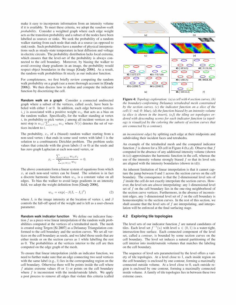
Figure 4: Topology exploration: (a) a cell with 4 section curves, (b)the boundary-conforming Delaunay tetrahedral mesh constrainedby the section curves, (c) the indicator function on a slice of thecell (1: red; 0: blue), (d) the function biased by an intensity volume(a slice is shown in the insert), (e,f) the tiling set topologies or-dered with descending scores for each indicator function (a topol-ogy is visualized by the coloring the subsets of section curves thatare connected by a contour).
an inconsistent edge) by splitting each edge at their midpoints andsubdividing their incident faces and tetrahedra.
An example of the tetrahedral mesh and the computed indicatorfunction f is shown for a 3D cell in Figure 4 (b,c,d). Observe that fcomputed in the absence of any additional intensity volume (shownin (c)) approximates the harmonic function in the cell, whereas theuse of the intensity volume strongly biased f so that its level setsare aligned with the intensity boundaries (shown in (d)).
An inherent limitation of linear interpolation is that it cannot cap-ture the jump between 0 and 1 across the section curves on the cellboundary. The consequence is that the 2-dimensional level sets off inside the cell do not exactly interpolate the section curves. How-ever, the level sets are almost interpolating: any 1-dimensional levelset of f on the cell boundary lies in the one-ring neighborhood ofthe section curve vertices. Furthermore, in the absence of inconsis-tent edges, any 1-dimensional level set of f on the cell boundary ishomeomorphic to the section curves. In the rest of this section, weshall assume that the level sets of f are interpolating, and interpo-lation will be enforced at the final surfacing stage.
4.2 Exploring tile topologies
The level sets of our indicator function f are natural candidates oftiles. Each level set f−1(u) with level u ∈ (0, 1) is a water-tight,intersection-free surface. Each connected component of the levelset, called a contour, is bounded by some section curves on thecell boundary. The level set induces a natural partitioning of thecell interior into inside/outside volumes that matches the labelingon the cell boundary.
The sequence of level sets parameterized by the level offers a vari-ety of tile topologies. At a level close to 1, each inside region onthe cell boundary is enclosed by one contour, forming a maximallyconnected outside volume. At a level close to 0, each outside re-gion is enclosed by one contour, forming a maximally connectedinside volume. A family of tile topologies lies in between these twoextreme cases.

(a) (b) (c)
Figure 5: Level sets topology in 2D: (a) A rectangular cell with 6 inside regions (Ii) and 6 outside regions (Oi) on the cell boundary, thecontours of the indicator function (colored by their levels), and a tiling set (ci). (b) The critical points (a, b, c, d, e) and the contours thatcontain them (black lines). These contours divide the cell into regions of contours with a common topology. (c) The contour tree that capturesthe critical points as nodes and regions as edges.
To further enrich this family, we also consider contours at differentlevels. Note that any set of contours, regardless of their levels, areclosed and intersection-free. To form a valid tile, we only need torequire that each section curve is used by exactly one contour. Wecall a set of contours that meet this requirement a tiling set. Anylevel set is a tiling set. Just like a level set, a tiling set partitions thecell interior into inside/outside volumes.
Tiling sets offer a wider range of topologies than level sets. This isparticularly important in the scenario where the object to be recon-structed contains multiple components in the cell and the topologyof each component is only realized by level sets at different lev-els. We illustrate this case in the 2D example in Figure 5. Herewe consider a rectangular cell bounded by four cross-section lines.The cell boundary is partitioned into several inside regions (Ii) andoutside regions (Oi). An intuitive reconstruction within the cellwould be three “tubes” that connect the three pairs of inside regions{I1, I4}, {I2, I5} and {I3, I6}. The level sets of the indicator func-tion with distinct topology are illustrated by colored curves, wherecontours at the same level are colored the same. Note that no singlelevel set has the desired 3-tube connectivity. This is because the pair{I3, I6} is smaller than and further away from the other two pairs.Any level set that connects this pair into a tube (e.g., blue) wouldcause the other two pairs to be merged into a single branching tube.On the other hand, the 3-tube connectivity can be achieved by thetiling set consisting of contours c1, . . . , c6 at two different levels.
Our exploration proceeds in two steps. First we will enumeratedistinct contour topologies, and they will be combined in a secondstep to form topologies of tiling sets.
Topology of simple contours We start by enumerating all pos-sible contour topologies in our indicator function. Such topologiesare captured by the contour tree [van Kreveld et al. 1997], which isa directed tree-like graph that captures the evolution of the contourtopology as the level changes. Each node in the tree corresponds toa critical point in the function and each edge corresponds to a set ofcontours with a common topology (an example is shown in Figure5 (c)). We use the algorithm in [van Kreveld et al. 1997] to computethe contour tree, which also gives the topology information for eachedge of the tree. We encode each distinct contour topology by itsgenus and bounding section curves.
In our experiment, we observed that a large number of contourtopologies have genus greater than zero. These topologies signifi-cantly increase the number of tiling set topologies that we will ex-plore next, and they are rarely selected to be used on the final re-construction. To improve efficiency, we make the assumption thatany topological feature of the object (e.g., handles) is sampled bysome cross-section, and hence we only consider contours within acell that are simple, or has zero genus. Note that relaxing this re-striction does not pose any difficulty to the rest of the algorithm.
Topology of tiling sets Given the contour topologies, we nextenumerate ways in which they can be combined to form tiling sets.Recall that a set of contours is a tiling set if each section curve onthe cell boundary bounds exactly one contour in the set. The taskof finding tiling sets can therefore be formulated as an exact coverproblem as follows. Suppose we have a set of section curves Cand a collection of contour topologies T = {t1, . . . , tm}, whereeach ti is a subset of C that bound the contour. Our goal is find asub-collection T ′ ⊆ T such that each curve in C is appears exactlyonce in some subset in T ′.
The exact cover problem is one of Karp’s 21 NP-complete prob-lems. Kunth’s Dancing Link algorithm [Knuth 2000] can be usedto find all possible solutions, but its running time may scale expo-nentially with the input size. In our implementation, however, wefound that Dancing Link runs sufficiently fast (e.g., within a sec-ond) for finding tiling set topologies in all our test examples.
4.3 Scoring
To evaluate the “naturalness” of a tile topology, we again makeuse of our indicator function which approximates the random-walkprobability. Conceptually, we consider the inside/outside labellingof the cell interior imposed by a tile, and score the tile by the jointlikelihood of the label at each point. We first present our defini-tion of the score function for any given tile in the cell (not limitedto tiling sets of the indicator function). Then we discuss how thescore is computed for a topology of a tiling set.
Scoring an arbitrary tile To measure the likelihood of a tile Tas a labelling of the cell space, we first calculate the likelihood ofthe labeling at a point x inside the cell. Let f be the random-walkprobability, and lT be the label at x as determined by the tile T .The likelihood of the label at x given tile T can be formulated as
hT (x) =
{log(f(x)) if lT (x) is insidelog(1 − f(x)) if lT (x) is outside (3)
We use the logarithm so that the joint-likelihood of multiple pointscan be calculated by summation. Integrating the per-point likeli-hood over the entire cell space Ω gives the continuous formulationof our score for the tile T ,
h(T ) =
∫Ω
hT (x)dx. (4)
In practice, we compute the score discretely over the vertices V ofthe tetrahedral mesh. To compensate for the variation in tetrahedrasizes in different cells, we compute the following weighted sum
h(T ) =∑v∈V
hT (v)w(v). (5)

where w(v) is the sum of volumes of tetrahedra incident to vertexv. Since w(v) can be pre-computed from the mesh structure, theonly computation involved in scoring a given tile is computing theinside/outside label LT (v) for each vertex v from the tile.
Scoring a tiling set topology Given a tiling set topology, weneed to pick one tiling set that realizes the topology in order tocompute the score. This amounts to finding a representative con-tour for each contour topology. Ideally, the representative contourshould maximize the score. Note that our score function increaseswhen an inside point x where f(x) < 0.5 changes its label to out-side or when an outside point y where f(y) > 0.5 changes its labelto inside. Hence replacing a contour by another (with the sametopology) whose level is closer to 0.5 always increases the score.
With this observation, we define the representative contour for eachcontour topology as one whose level is closest to 0.5. Specifically,suppose the range of levels of the contour topology is [ul, uh] (thisinformation is readily available on the contour tree). If the rangecontains the value 0.5, we shall use the contour at level 0.5. Oth-erwise, we use the contour at level ul + ε if ul > 0.5 and at leveluh−ε otherwise, where ε is a small value so that the contour avoidsthe critical points.
Figure 4 (e) shows all tiling set topologies found in the indica-tor function in (c), ranked by their scores. Note that the familyof topologies captures a range of connections between the sectioncurves, from one that disconnects all section curves (#1) to one thatconnects all of them (#4). On the other hand, the use of the inten-sity volume encourages topologies (f) that are better aligned withthe strong intensity boundaries, many of which are not present inthe original family (e).
5 Topology selection
Given a set of tile topologies with scores within each cell, we needto choose one topology per cell so that their union is a surfacewith a single connected component and the user-specified genusgu. In addition, we seek the choice that has the maximal cumu-lative scores among all possible choices. We call such choice theoptimal tiling. We solve this combinatorial optimization using abottom-up dynamic programming algorithm, which is guaranteedto find the global optimum. Note the algorithm is independent fromhow the tile topologies are generated or scored within the cells.
5.1 A dynamic programming problem
Before presenting the algorithm, we first need to show that the prob-lem of finding optimal tiling has the required properties to be solvedby dynamic programming, namely optimal substructure and over-lapping subproblems.
We consider a more general problem as follows. Given a volumeV formed by the union of a collection of cells, we seek the optimaltiling for cells in V constrained by a given topology T . Here, T isrepresented by its connected components, and each component isencoded by its genus and the (possibly empty) subset of the sectioncurves on the boundary of V that bound the component. We denotethe score of the optimal tiling as h(V, T ). Our topology selectionproblem is simply finding h(V, T ) (and the per-cell tile topologiesthat achieve this score) when V is the union of all cells and T con-tains a single component with genus gu.
To see that the problem has an optimal substructure, consider anydecomposition of V into sub-volumes V1, V2 that are unions of sub-sets of the cells in V . There could be multiple ways to choose a
surface topology in each sub-volume, say T1, T2, so that the topol-ogy of the union of the two surfaces, denoted as T1 ∨ T2, has thedesired topology T . This is illustrated in the 2D example in Figure6. Since the score of a tile topology in one cell is independent fromthe other cells, we can write h(V, T ) as the maximum sum of thescores over all possible combinations of T1, T2:
h(V, T ) = maxT1∨T2=T
(h(V1, T1) + h(V2, T2)) (6)
Moreover, note that each subproblem h(Vi, Ti) may be used indefining h(V, T ) for different choices of topology constraints T .Hence a dynamic programming algorithm is suited for finding h.
=,
+ ++,{
Figure 6: A 2D illustration that the topology in a volume V1 ∪V2 (left) can be achieved by multiple combinations of topologiesin each sub-volume V1 and V2 (right). The thick black segmentsdenote the inside region on the boundary of the volume.
5.2 A bottom-up algorithm
We perform dynamic programming in a bottom-up fashion, incre-mentally computing the solution within an increasingly larger unionof cells. Given some ordering of the cells, we start from the firstcell as the initial known volume and grow this volume by taking theunion with subsequent cells. As we expand V , we incrementallyupdate and store h(V, T ) (and the optimal tiling) for all possiblesurface topology T within V . Suppose V1 is the previous knownvolume and V2 is the newly added cell, such that V = V1 ∪V2. Weenumerate all combinations of any topology T1 stored at V1 and anytile topology T2 given in the cell V2. We then use the recurrencein Equation 6 to compute h(V, T ) for all distinct union topologiesT = T1 ∨ T2. After all cells are included in the known volumeV , we output the value h(V, T ) where T has a single connectedcomponent with the user-specified genus gu.
A key element of the algorithm is the topological union operation∨, which we shall elaborate first. We then discuss ways to improvethe efficiency of the basic algorithm.
Topological union Given two surface topologies T1, T2, eachconsisting of one or more components, we first need to know whichof these components are merged to a single component in the uniontopology T = T1∨T2. Note that a component in T1 is merged witha component in T2 if the two components share some common por-tion of their boundaries. We call these two components boundary-connected. Hence a component of T is a maximally boundary-connected set of components in T1 and T2.
For each component t of T , our next task is to compute its genus(gt) and boundary curves (Bt) from those of the un-merged com-ponents in T1 and T2. Suppose t is made up of m components t1i inT1 for i = 1, . . . , m each with genus g1
i and boundary curves B1i ,
and n components t2j in T2 for j = 1, . . . , n each with genus g2j
and boundary curves B2j .
Since merging happens along boundaries, the portion of any B1i
(resp. B2j ) that remains on the boundary of the merged surface Bt
is precisely the portion that is not shared by any B2j (resp. B1
i ).Hence we can obtain Bt using the symmetric difference operator⊕,
Bt = (∪mi=1B
1i ) ⊕ (∪n
j=1B2j ). (7)

To compute the genus gt, we resort to the Euler formula for a con-nected surface with boundary,
gt = (2 − ‖Bt‖ − χt)/2, (8)
where ‖Bt‖ denotes the number of loops in Bt, and χt is the Eulercharacteristics of t, which is computed as the sum of the number ofvertices and number of faces minus the number of edges. Note thatχt is the sum of Euler characteristics of the component surfacesadjusted by discounting those vertices and edges that are shared bydifferent boundary curves. Let us denote the Euler characteristicsfor each component t1i or t2j as χ1
i or χ2j (which can be computed
from {g1i , B1
i } or {g2j , B2
j } using the Euler formula above). Wehave
χt =m∑
i=1
χ1i +
m∑j=1
χ2j + e(L) − v(L). (9)
Here v and e respectively count the number of vertices and edgesof a graph, and L is the shared portions of the boundary curves,
L = (∪mi=1B
1i ) ∩ (∪n
j=1B2j ). (10)
The calculation of gt and Bt is illustrated in Figure 7. In this exam-ple, two components from T1 (t11, t12) and one component from T2
(t21) are merged. One of the boundary curves of t21 completely over-laps a boundary curve of t12, and another overlaps partly with twoboundary curves of t11 and t12 (marked by red arrows). The symmet-ric difference in Equation 7 gives three curves on the boundary oft. To calculate the genus, note that the overlapping portion of theboundary curves is made up of a closed loop and two open curves,hence e(L) − v(L) = −2. Also, using Euler formula we haveχ1
1 = χ12 = 0 and χ2
1 = −1. Applying Equation 9 gives Eulercharacteristic χt = −3, and applying Equation 8 yields gt = 1,which correctly captures the presence of a topological handle on t.
Figure 7: Merging surfaces along their boundaries (green).Complexity and acceleration The time complexity of dynamicprogramming is upper bounded by the product of three quanti-ties, the total number of cells (ncell), the maximum number of tiletopologies explored within any cell (ntile), and the maximum num-ber of topologies of tile unions that the algorithm creates in a knownvolume (nunion). The algorithm stores, for each union topologywithin a known volume, the optimal tiling of that topology whichconsists of one tile topology per cell. Hence the space usage isupper bounded by ncell × nunion.
The quantity nunion is the dominating factor of both time and spacecomplexity. This number can be easily exponential on the numberof section curves on the known volume’s boundary. We propose twoways to tame the complexity. First, we use a greedy strategy to findthe expansion order of cells that would reduce the number of sectioncurves on the known volume. Specifically, the cell to be expandednext is selected as one among all remaining cells adjacent to theknown volume that would yield the minimum number of sectioncurves on the boundary of the expanded known volume. Second,we can prune those topologies that are inconsistent with the goal.Note that any topological handle or closed surface created during
the algorithm will remain so throughout the expansion of the knownvolume. Since our final output is a single component with genus gu,we prune all topologies that either contain closed surfaces or havegenus greater than gu at each step of dynamic programming.
We observed that, in a real-world reconstruction scenario (such assegmenting a biological shape), the object to be recovered usuallyhas a low genus and the number of curves on each cross-sectionplane tends to be small. In this case, the combination of our cellordering and pruning strategies can successfully reduce nunion to asmall amount such that dynamic programming runs efficiently. Asshown in Section 7, topology selection takes negligible time for allexamples in this paper.
Nonetheless, the computational cost can become prohibitive if theobject has a high topological complexity and each plane contains alarge number of curves (e.g., a porus material or a neural network).To be able to handle these inputs, one could trade off optimalityfor efficiency by keeping only the top k topologies (as measuredby their scores) in the known volume at each step of the expan-sion, where k is a user-supplied constant. This simple modificationwould make the algorithm run in time (and space) linear to the num-ber of cells, regardless of the complexity of the input or the object,but possibly resulting in sub-optimal solutions.
6 Surfacing
Having found the optimal choice of tile topology per cell, we nextneed to construct the geometry of the tiles that realize those topolo-gies. Ideally, the tile geometry should smoothly interpolate the in-put contours. A natural candidate is the set of representative con-tours that we used to score each tiling set topology (see Section4). The geometry of these contours can be extracted as a piece-wise linear surface using an iso-surfacing algorithm (e.g., marchingtetrahedra) on the tetrahedral mesh.
While these contours possess the desired topology, they cannot bedirectly used as the final result for two reasons. First, as men-tioned earlier, the contours within a cell don’t exactly interpolatethe section curves on the cell boundary. To enforce interpolation,we snap the boundary curves of a contour to the corresponding sec-tion curves. This can be done during the extraction of the contour.Recall the marching tetrahedra algorithm creates one contour ver-tex on each mesh edge that crosses the segment. If this edge lieson the cell boundary and only one of the edge’s end point lies on asection curve, we simply use that end point as the contour vertex onthat edge. Figure 8 (b,c) shows an example of contours extractedwithout and with snapping.
Second, the contours may exhibit a jagged appearance, in part dueto the resolution of the tetrahedral mesh. Also, since the geometryof the contour in one cell is determined independently from con-tours in adjacent cells, simply gluing contours from different cellsmay not create a smooth overall shape. Following previous work[Liu et al. 2008], we improve the quality of the merged surface it-eratively by alternating between Delaunay-based mesh refinement[Liepa 2003] and fairing based on surface-diffusion flow [Xu et al.2006]. Both refinement and fairing are constrained by the sectioncurves to maintain the interpolation property. An example result ofmesh improvement is shown in Figure 8 (d).
7 Results
We test the ability of our algorithm in controlling surface topologyon a variety of synthetic and real-world examples. We comparewith the results of two leading methods by Bermano et al. [2011]

Figure 8: Surfacing: (a) two cross-sections, (b) surface computedwithout snapping to section curves, (c) with snapping enabled, (d)after quality improvement.
and by Lu et al. [2008]. Both methods can be regarded as tak-ing a fixed level set of some indicator function defined within acell, where the function is obtained by mean-value interpolation(in Bermano’s method) or nearest-neighbor interpolation (in Lu’smethod). Besides the difference in the choice of the indicator func-tion, our method considers a family of contour topologies per celland strives to achieve a prescribed genus. While we focus on topo-logical correctness in the comparisons, we note that these two meth-ods offer additional features that our method is lacking, such ashandling multi-labelled cross-sections and even missing labels.
Figure 9 examines the impact of cross-section sampling density onvarious methods using a synthetic torus. Without resorting to im-age data, our algorithm is able to produce surfaces with the desiredgenus (i.e. 1) in all three sampling densities (shown in column (d)).However, it fails to capture the torus structure in the sparsest input(bottom row). A closer look at a middle cell (see Figure 4) revealsthat the correct tile topology in the cell, which should consist of twoseparate tubes, is missing in the tiling sets of our indicator function.Such tile topology can be recovered by incorporating a syntheticdensity volume (shown in the top-right), which allows our methodto create surfaces with both correct topology and structure (shownin column (e)). Note that the synthetic volume was intentionallymade noisy to mimic the quality of typical biomedical data. Wealso show (in (e) of bottom row) the result of our method with adifferent target genus (0), in which the torus is broken where thesynthetic density is low in the volume.
In comparison, the other two methods produce topological errorsfor even denser inputs. As discussed earlier and observed in Figure3, Lu’s algorithm easily creates connections (resp. disconnections)between section curves whose projections are barely overlapping(resp. disjoint). On the other hand, Bermano’s method appearsto create the most disconnections, implying that the method mightrequire a rather dense sampling to maintain the connectivity of thereconstruction.
Similar observations can be made in the chicken heart examplesshown earlier. Our algorithm is able to recover the correct topologywhen the cross-sections are too sparse for the other two methodsto succeed (Figure 1), and we can handle even fewer cross-sectionswhen the original CT image is utilized (Figure 2).
Finally, we tested our algorithm (without the use of any additionalimages) on several more complex inputs depicting both everydayobjects and biological structures, shown in Figure 11. These objectsall contain thin sheets (e.g., mug and hip bone) or tubes (e.g., handand vertebrae), which are challenging for existing methods. Ouralgorithm on the other hand is able to create a single connectedsurface with the desired (non-zero) genus.
Figure 9: Cross-sections of a torus at different sampling densities(a) and the reconstructed surfaces using the method of Lu et al.[2008] (b), Bermano et al. [2011] (c), our method with genus-1constraint without additional image data (d), and our method usinga synthetic but noisy image (shown in the top insert) (e).
Performance Our algorithm was implemented in C++ and testedon a 12-core 2.4Ghz PC with 12G main memory. During topol-ogy exploration step, exploration in different cells is executed inparallel. Our implementation runs from a few seconds to less thantwo minutes for all examples shown in the paper (see last columnof Figure 11). This run time is dominated by iterative fairing andrefinement during the final surfacing, which in turn depends on thetriangle count. Topology exploration finishes within seconds for allexamples, while topology selection takes negligible time.
We further examined the performance of the dynamic programmingalgorithm for topology selection under varying factors such as thenumber of cross-section planes and target genus. Our input is a setof parallel cross-sections of a Trefoil knot (Figure 10 left). Notethat there could be up to 8 section curves on the boundary of a celland up to 5 section curves the boundary of the known volume dur-ing dynamic programming. We varied the number of cross-sectionplanes from 6 to 55 and the target genus from 0 to 3. As seen inFigure 10 right, the running time of the algorithm increases almostlinearly both with the number of planes and the target genus. Evenwith more than 50 planes and a target genus of 3, the algorithmfinished in under a second.
Figure 10: Left: reconstruction of Trefoil knot from 6 cross-sectionplanes with target genus 1. Right: running time of topology selec-tion with increasing number of planes for different target genuses.
8 Conclusion and discussion
We present, to our best knowledge, the first algorithm for control-ling the topology of the surface when reconstructing from planarcross-sections. We solve the problem in two stages, first generatinga family of topologies within each cell of the plane arrangement,

Figure 11: Reconstructions from input cross-sections (a) using the method of Lu et al. [2008] (b), method of Bermano et al. [2011] (c), andour method with prescribed genuses without additional image data (showing running times) (d).
then optimally selecting one topology per cell. The algorithm isshown on several examples to be able to capture the correct topol-ogy using fewer cross-sections than previous algorithms.
The diversity of per-cell tile topologies and the quality of theirscores, as the result of the first stage, directly impact the final resultof our algorithm. Our strategy of restricting the tiles to the contoursof an indicator function seems to offer a reasonable sampling of thetopology space while maintaining computational efficiency. How-ever, our limited sampling may not contain the desired tile topologywhen the spacing of the cross-sections is too sparse (see Figures 2and 9). A wider range of tile topologies and better scoring func-tions may lead to more accurate outputs, but at the possible cost ofsubstantially increased computation time. Alternatively, it wouldalso be interesting to explore a way that allows the user to specifydesired tile topology in ambiguous cells.
Finally, we envision that our two-stage paradigm can be extended tooffer topology control in other applications involving surface recon-struction, such as from point clouds or scalar functions. The “cells”would be isolated volumes where there is ambiguity in the topol-ogy of the reconstructed surface (e.g., near the critical points of thescalar function [Sharf et al. 2007]). By exploring possible topolo-gies within each cell, and scoring them appropriately, our topologyselection algorithm can be used to pick the optimal topology percell that achieves a global genus constraint.
Acknowledgement This work is supported in part by NSF grants(IIS-1302200 and IIS-0846072) and a gift from Adobe.
References
AMINI, O., BOISSONNAT, J., AND MEMARI, P. 2013. Geometrictomography with topological guarantees. Discrete & Computa-

tional Geometry 50, 4, 821–856.
ATTENE, M., CAMPEN, M., AND KOBBELT, L. 2013. Polygonmesh repairing: An application perspective. ACM Comput. Surv.45, 2 (Mar.), 15:1–15:33.
BAJAJ, C. L., COYLE, E. J., AND LIN, K.-N. 1996. Arbi-trary topology shape reconstruction from planar cross sections.Graph. Models Image Process. 58, 6, 524–543.
BAREQUET, G., AND SHARIR, M. 1996. Piecewise-linear inter-polation between polygonal slices. Computer Vision and ImageUnderstanding 63, 251–272.
BAREQUET, G., AND VAXMAN, A. 2007. Nonlinear interpola-tion between slices. In SPM ’07: Proceedings of the 2007 ACMsymposium on Solid and physical modeling, 97–107.
BAREQUET, G., AND VAXMAN, A. 2009. Reconstruction ofmulti-label domains from partial planar cross-sections. Comput.Graph. Forum 28, 5, 1327–1337.
BAREQUET, G., GOODRICH, M. T., LEVI-STEINER, A., ANDSTEINER, D. 2004. Straight-skeleton based contour interpo-lation. Graph. Models 65, 323–350.
BAREQUET, G., GOTSMAN, C., AND SIDLESKY, A. 2006. Poly-gon reconstruction from line cross-sections. In Proceedings ofthe 18th Annual Canadian Conference on Computational Ge-ometry, CCCG 2006, August 14-16, 2006, Queen’s University,Ontario, Canada.
BAZIN, P., AND PHAM, D. L. 2007. Topology-preserving tissueclassification of magnetic resonance brain images. IEEE Trans.Med. Imaging 26, 4, 487–496.
BERMANO, A., VAXMAN, A., AND GOTSMAN, C. 2011. Onlinereconstruction of 3d objects from arbitrary cross-sections. ACMTrans. Graph. 30, 5 (Oct.), 113:1–113:11.
BOISSONNAT, J.-D., AND MEMARI, P. 2007. Shape reconstruc-tion from unorganized cross-sections. In SGP ’07: Proceedingsof the fifth Eurographics symposium on Geometry processing,89–98.
BOISSONNAT, J.-D. 1988. Shape reconstruction from planar crosssections. Comput. Vision Graph. Image Process. 44, 1, 1–29.
CHENG, S.-W., AND DEY, T. K. 1999. Improved constructionsof delaunay based contour surfaces. In SMA ’99: Proceedingsof the fifth ACM symposium on Solid modeling and applications,ACM Press, 322–323.
FUCHS, H., KEDEM, Z. M., AND USELTON, S. P. 1977. Optimalsurface reconstruction from planar contours. Commun. ACM 20,10, 693–702.
GRADY, L. 2006. Random walks for image segmentation. IEEETrans. Pattern Anal. Mach. Intell. 28, 11 (Nov.), 1768–1783.
HERMAN, G. T., ZHENG, J., AND BUCHOLTZ, C. A. 1992.Shape-based interpolation. IEEE Comput. Graph. Appl. 12, 3,69–79.
IJIRI, T., YOSHIZAWA, S., YOKOTA, H., AND IGARASHI, T.2014. Flower Modeling via X-ray Computed Tomography. ACMTrans. Graph. 33, 4, to appear. Proc. of SIGGRAPH’14.
JU, T., WARREN, J. D., CARSON, J., EICHELE, G., THALLER,C., CHIU, W., BELLO, M., AND KAKADIARIS, I. A. 2005.Building 3d surface networks from 2d curve networks with ap-plication to anatomical modeling. The Visual Computer 21, 8-10,764–773.
KEPPEL, E. 1975. Approximating complex surfaces by triangula-tion of contour lines. IBM Journal of Research and Development19, 1, 2–11.
KNUTH, D. E. 2000. Dancing links. Millenial Perspectives inComputer Science (Nov), 187–214.
LIEPA, P. 2003. Filling holes in meshes. In Proceedings of the 2003Eurographics/ACM SIGGRAPH Symposium on Geometry Pro-cessing, Eurographics Association, Aire-la-Ville, Switzerland,Switzerland, SGP ’03, 200–205.
LIU, L., BAJAJ, C., DEASY, J., LOW, D. A., AND JU, T. 2008.Surface reconstruction from non-parallel curve networks. Com-put. Graph. Forum 27, 2, 155–163.
MEYERS, D., SKINNER, S., AND SLOAN, K. 1992. Surfaces fromcontours. ACM Trans. Graph. 11, 3, 228–258.
OLIVA, J.-M., PERRIN, M., AND COQUILLART, S. 1996. 3d re-construction of complex polyhedral shapes from contours usinga simplified generalized voronoi diagram. Computer GraphicsForum 15, 3, 397–408.
SHARF, A., LEWINER, T., SHKLARSKI, G., TOLEDO, S., ANDCOHEN-OR, D. 2007. Interactive topology-aware surface re-construction. ACM Trans. Graph. 26, 3 (July).
SI, H., 2007. TetGen. a quality tetrahedral mesh generator andthree-dimensional delaunay triangulator.
TURK, G., AND O’BRIEN, J. F. 1999. Shape transformation usingvariational implicit functions. In SIGGRAPH ’99: Proceedingsof the 26th annual conference on Computer graphics and inter-active techniques, ACM Press/Addison-Wesley Publishing Co.,335–342.
VAN KREVELD, M., VAN OOSTRUM, R., BAJAJ, C., PASCUCCI,V., AND SCHIKORE, D. 1997. Contour trees and small seed setsfor isosurface traversal. In Proceedings of the Thirteenth AnnualSymposium on Computational Geometry, SCG ’97, 212–220.
WOOD, Z. J., HOPPE, H., DESBRUN, M., AND SCHRODER, P.2004. Removing excess topology from isosurfaces. ACM Trans.Graph. 23, 2, 190–208.
XU, G., PAN, Q., AND BAJAJ, C. 2006. Discrete surface mod-elling using partial differential equations. Computer Aided Geo-metric Design 23, 2, 125–145.
YIN, K., HUANG, H., ZHANG, H., GONG, M., COHEN-OR, D.,AND CHEN, B. 2014. Morfit: Interactive surface reconstruc-tion from incomplete point clouds with curve-driven topologyand geometry control. ACM Trans. Graph. 33, 6 (Nov.), 202:1–202:12.
ZENG, Y., SAMARAS, D., CHEN, W., AND PENG, Q. 2008.Topology cuts: A novel min-cut/max-flow algorithm for topol-ogy preserving segmentation in N-D images. Computer Visionand Image Understanding 112, 1, 81–90.
ZHOU, Q.-Y., JU, T., AND HU, S.-M. 2007. Topology repair ofsolid models using skeletons. IEEE Transactions on Visualiza-tion and Computer Graphics, to appear.
ZHOU, S., JIANG, C., AND LEFEBVRE, S. 2014. Topology-constrained synthesis of vector patterns. ACM Transactions onGraphics (Proc. SIGGRAPH Aisa) 33.


