CHAPTER 26
Systemic Contingent Claims Analysis
ANDREAS A. JOBST • DALE F. GRAY
This chapter introduces a new framework for macroprudential analysis using a risk- adjusted balance sheet approach that supports policy eff orts aimed at mitigating systemic risk from linkages between institutions and the extent to which they precipitate or amplify general market dis-
tress. In this regard, a forward- looking framework for mea sur ing systemic solvency risk using an advanced form of contingent claims analysis (CCA), known as “Systemic CCA,” is presented for the systemwide capital assessment in top- down stress testing. The magnitude of joint default risk of multiple fi nancial institutions falling into distress is modeled as a portfolio of individual market- implied expected losses (with individual risk pa ram-e ters) calculated from equity market and balance sheet information. An example of Systemic CCA applied to the U.K. banking sector delivers useful insights about the magnitude of systemic losses in the context of macroprudential stress testing. In addition, the framework also helps quantify the individual contributions of institutions to systemic risk of the fi nancial sector during times of stress.
METHOD SUMMARY
Overview The Systemic Contingent Claims Analysis (Systemic CCA) model extends the traditional risk- adjusted balance sheet model (based on contingent claims analysis) to analyze systemic risk from the interlinkages among institutions, including time- varying dependence of default risk. This approach helps quantify the contribution of individual institutions to systemic (sol-vency) risk and to assess spillover risks from the fi nancial sector to the public sector (and vice versa). In addition, Systemic CCA can be applied to macroprudential stress testing using the historical dynamics of market- implied expected losses.
Application The method is appropriate in situations where access to prudential data is limited but market information is readily available.
Nature of approach Model- based (option pricing, multivariate parametric/nonparametric estimation, credit default swap [CDS] curve pricing).
Data requirements • Accounting information (amounts/maturities) of outstanding liabilities. • Market data on equity and equity option prices. • Various market rates and macro data for satellite model underpinning the stress test. • Sovereign CDS term structure/debt level and debt repayment schedule (if fi nancial sector- sovereign spillover risk is
tested).
Strengths • The model integrates market- implied expected losses (and endogenizes loss given default) in a multivariate specifi cation of joint default risk.
• The approach is highly fl exible and can be used to quantify an individual institution’s time- varying contribution to sys-temic solvency risk under normal and stressed conditions.
Weaknesses • Assumptions are required regarding the specifi cation of the option pricing model (for the determination of implied asset and asset volatility of fi rms).
• Technique is complex and resource intensive.
Tool The Excel VBA- based tool is available with this book. Contact author: A. Jobst.
Large parts of the material in this chapter are published in the Sveriges Riksbank Economic Review, No. 2, pp. 68– 106 (Gray and Jobst, 2011b) and IMF Working Paper 13/54 ( Jobst and Gray, 2013).
536-57355_IMF_StressTestHBk_ch03_3P.indd 409 11/5/14 2:06 AM
Systemic Contingent Claims Analysis 410
former, the contribution to systemic risk arises from the initial eff ect of direct exposures to the failing institution (e.g., defaults on liabilities to counterparties, investors, or other market par-ticipants), which could also spill over to previously unrelated institutions and markets as a result of greater uncertainty or the reassessment of fi nancial risk (i.e., changes in risk appetite and/or the market price of risk). Table 26.1 summarizes the distinguishing features of both approaches.
Th e growing literature on systemic risk mea sure ment has responded to greater demand placed on the ability to develop a better understanding of the interlinkages between fi rms and their implications for fi nancial stability (see Table 26.2). Th e specifi cation of dependence between fi rms helps identify common vulnerabilities to risks as a result of the (assumed) collective behavior under common distress ( Jobst, 2013). Most of the prominent institution- level mea sure ment approaches have focused on the contribution approach by including an implicit or explicit treatment of statistical dependence in de-termining joint default risk or expected losses. For instance, Acharya, Pedersen, and others (2009, 2010, 2012) estimate potential losses as marginal expected shortfall (MES) of in-dividual banks in the event of a systemic crisis, which is de-fi ned as the situation when the aggregate equity capital of sample banks falls below some fraction of aggregate assets. Brownlees and Engle (2011) apply the same defi nition for a systemic crisis and formulate a capital shortfall mea sure (“SRISK index”) that is similar to MES; however, they pro-vide a closed- form specifi cation of extreme value dependence underpinning MES by modeling the correlations between the fi rm and market returns using the dynamic conditional correlation (DCC)- GARCH model (Engle and Sheppard, 2001; Engle, 2002). Also, Huang, Zhou, and Zhu (2009, 2010) derive correlation of equity returns via DCC- GARCH as statistical support to motivate the specifi cation of the dependence structure for default probabilities within a sys-tem of fi rms. Both CoVaR and CoRisk (Adrian and Brun-nermeier, 2008; Chan- Lau, 2010) follow the same logic of deriving a bivariate mea sure of dependence between a fi rm’s fi nancial per for mance and an extreme deterioration of market conditions (or that of its peers). For instance, the CoVaR (CoRisk) for a certain fi rm is defi ned as the value at risk (VaR) (as a mea sure of extreme default risk) of the whole sector (fi rm) conditional on a par tic u lar institution being in distress.
However, only a few models estimate multivariate (fi rm- by- fi rm) dependence through either a closed- form specifi ca-tion or the simulation of joint probabilities using historically informed mea sures of association. None of those include a structural defi nition of default risk. A chapter of a recent issue of the Global Financial Stability Report provides comparative analysis of several of these systemic risk mea sures in the con-text of designing early- warning indicators for MPS (IMF,
institution being part of it, which determines the institution’s marginal contribution to systemic risk.
In the wake of the global fi nancial crisis, there has been in-creased focus on systemic risk as a key aspect of macro- prudential policy and surveillance (MPS) with a view toward enhancing the resilience of the fi nancial sector.1 MPS is pred-icated on (1) the assessment of systemwide vulnerabilities and the accurate identifi cation of threats arising from the buildup and unwinding of fi nancial imbalances, (2) shared exposures to macro- fi nancial shocks, and (3) possible conta-gion/spillover eff ects from individual institutions and mar-kets owing to direct or indirect connectedness. Th us, it aims to limit, mitigate, or reduce systemic risk, thereby minimizing the incidence and impact of disruptions in the provision of key fi nancial ser vices that can have adverse consequences for the real economy (and broader implications for economic growth). Systemic risk refers to individual or collective fi -nancial arrangements— both institutional and market- based—which could either lead directly to systemwide distress in the fi nancial sector or signifi cantly amplify its conse-quences (with adverse eff ects on other sectors, in par tic u lar capital formation in the real economy). Typically, such dis-tress manifests itself in disruptions to the fl ow of fi nancial ser vices because of an impairment of all or parts of the fi -nancial system that are deemed material to the functioning of the real economy.2
Although there is still no comprehensive theory of MPS re-lated to the mea sure ment of systemic risk, existing approaches can be distinguished broadly on the basis of their conceptual underpinnings regarding several core principles. Th ere are two general approaches: (1) a par tic u lar activity causes a fi rm to fail, whose importance to the system imposes marginal distress on the system owing to the nature, scope, size, scale, concentra-tion, or connectedness of its activities with other fi nancial in-stitutions (“contribution approach”), or (2) a fi rm experiences losses from a single (or multiple) large shock(s) because of a signifi cant exposure to the commonly aff ected sector, country, and/or currency (“participation approach”).3 In the case of the
1 In a progress report to the G20 (Financial Stability Board, International Monetary Fund, and Bank for International Settlements [FSB, IMF, and BIS], 2011a), which followed an earlier update on macro- prudential policies (FSB/IMF/BIS, 2011b), the FSB takes stock of the development of governance structures that facilitate the identifi cation and monitor-ing of systemic fi nancial risk as well as the designation and calibration of instruments for macroprudential purposes aimed at limiting sys-temic risk. Th e Committee on the Global Financial System (2012) pub-lished a report on operationalizing the selection and application of macroprudential policies, which provides guidance on the eff ectiveness and timing of banking sector– related instruments (aff ecting the treat-ment of capital, liquidity, and assets for the purposes of mitigating the cyclical impact of shocks and enhancing systemwide resilience to joint distress events). See Acharya, Cooley, and others (2010) as well as Acharya, Santos, and Yorulmazer (2010) for the implications of systemic risk in MPS in the U.S. context.
2 For a discussion of ways to assess the systemic importance of fi nancial institutions and markets, see IMF, FSB, and BIS (2009).
3 Drehmann and Tarashev (2011) refer to this as a “bottom- up approach,” whereas as a “top- down approach” would be predicated on the quantifi -cation of expected losses of the system, with and without a par tic u lar
536-57355_IMF_StressTestHBk_ch03_3P.indd 410 11/5/14 2:06 AM
Andreas A. Jobst and Dale F. Gray 411
Systemic CCA identifi es market- implied linkages aff ect-ing joint expected losses during times of stress, which can deliver important insights about the joint tail risk of multiple entities. A sample of fi rms (as proxy for an entire fi nancial system or parts thereof ) is viewed as a portfolio of individual expected losses (with individual risk pa ram e ters) whose sensi-tivity to common risk factors is accounted for by including the statistical dependence of their individual expected losses (“dependence structure”). Like other academic proposals, this approach helps assess individual fi rms’ contributions to systemic solvency risk (at diff erent levels of statistical con-fi dence). However, by accounting for the time- varying de-pendence structure, this method links the market- based assessment of each fi rm’s risk profi le with the risk characteris-tics of other fi rms that are subject to common changes in market conditions. Based on the expected losses arising from the variation of each individual fi rm’s expected losses, the joint probability of all fi rms experiencing distress simultane-ously can be estimated.
In addition, the Systemic CCA framework can generate closed- form solutions for market- implied estimates of capital adequacy under various stress test scenarios. By modeling how macroeconomic conditions and bank- specifi c income and loss elements (net interest income, fee income, trading income, operating expenses, and credit losses) have infl uenced the changes in market- implied expected losses (as mea sured by implicit put option values), it is possible to link a par tic u lar macroeconomic path to fi nancial sector per for mance in the future and derive estimates of joint capital needed to main-tain current capital adequacy. As a result, the market- implied joint capital need arises from the amount of expected losses relative to current (core) capital levels as well as its escalation
2011d).4 Th ere also are several studies on network analysis and agent- based models that are more closely related to the partici-pation approach by modeling how interlinked asset holdings matter in the generation and propagation of systemic risk (Al-len, Babus, and Carletti, 2010; Espinosa- Vega and Solé, 2011; Or ga ni za tion for Economic Cooperation and Development, 2012). Haldane and Nelson (2012) underscore this observa-tion by arguing that networks can produce nonlinearity and unpredictability with the attendant extreme (or fat- tailed) events.5
We propose a forward- looking, analytical, market data– based framework for estimating systemic risk in order to fi ll this gap in the literature. Th e suggested approach (“Systemic Contingent Claims Analysis” or “Systemic CCA”) extends the risk- adjusted (or economic) balance sheet approach to gener-ate estimates of the joint default risk of multiple institutions. Under this approach, the magnitude of systemic risk depends on the fi rms’ size and interconnectedness and is defi ned by the multivariate density of combined expected losses within a given system of fi nancial institutions.
4 A comparison of three mea sures of institution- level systemic risk exposure (Sedunov, 2012) suggests that CoVaR shows good forecasting power of the within- crisis per for mance of fi nancial institutions during two systemic crisis periods (Long- Term Capital Management in 1998 and Lehman Brothers in 2008). In contrast, Systemic Expected Shortfall (SES) is based on MES after considering diff erent degrees of fi rm leverage (Acharya, Ped-ersen, and others, 2012) and Granger causality does not seem to forecast the per for mance of fi rm per for mance reliably during crises.
5 One empirical example of the network literature is based on a Federal Reserve (Fed) data set, which allowed for the mapping of bilateral expo-sures of 22 global banks that accessed Fed emergency loans in the pe-riod 2008 to 2010 (Battiston and others, 2012). Th e authors fi nd that size is not a relevant factor to determine systemic importance.
TABLE 26.1
General Systemic Risk Mea sure ment ApproachesContribution approach (“Risk Agitation”) Participation approach (“Risk Amplifi cation”)
Concept Systemic resilience to individual failure Individual resilience to common shock
DescriptionA contribution to systemic risk conditional on
individual failure due to knock- on eff ectExpected loss from systemic event due to common
exposure and risk concentration
Risk transmission
“Institution- to- institution” “Institution- to- aggregate”Economic signifi cance of asset holdings (“size”) Claims on other fi nancial sector participants (credit
exposure)Intra- and intersystem liabilities (“connectedness”) Market risk exposure (interest rates, credit spreads,
currencies)
Risk indicators
Degree of transparency and resolvability (“complexity”)
Risk- bearing capacity (solvency and liquidity buff ers, leverage)
Participation in system- critical function/ser vice, e.g., payment and settlement system (“substitutability”)
Economic signifi cance of asset holdings, maturity mismatches debt pressure (“asset liquidation”)
Policy objectivesAvoid/mitigate contagion eff ect (by containing
systemic impact upon failure)Maintain overall functioning of system and maximize
survivorshipAvoid moral hazard Preserve mechanisms of collective burden sharing
Sources: Drehmann and Tarashev (2011); FSB, IMF, and BIS (2011a, 2011b); Jobst (2014); Tarashev, Borio, and Tsatsaronis (2009); and Weistroff er (2011).Note: The policy objectives and diff erent indicators to mea sure systemic risk under both contribution and participation approaches are not exclusive to each concept. Moreover, the availability of certain types of balance sheet information and/or market data underpinning the various risk indicators varies between diff erent groups of fi nancial institutions, which requires a certain degree of customization of the mea sure ment approach to the distinct charac-teristics of a par tic u lar group of fi nancial institutions.
536-57355_IMF_StressTestHBk_ch03_3P.indd 411 11/5/14 2:06 AM
Systemic Contingent Claims Analysis 412
TAB
LE 2
6.2
Sele
cted
Inst
itutio
n- Le
vel S
yste
mic
Ris
k M
odel
s
Des
crip
tio
nC
on
dit
ion
al V
alu
e at
Ris
k (C
oV
aR)
Co
nd
itio
nal
Ris
k (C
oR
isk)
SRIS
KSy
stem
ic E
xpec
ted
Sh
ort
fall
Dis
tres
s In
sura
nce
Pr
emiu
mJo
int P
rob
abili
ty o
f D
efau
ltSy
stem
ic C
on
tin
gen
t C
laim
s A
nal
ysis
Syst
emic
ris
k m
ea su
reVa
lue
at ri
skVa
lue
at ri
skEx
pec
ted
shor
tfal
lEx
pec
ted
sho
rtfa
llEx
pec
ted
sho
rtfa
llC
ond
itio
nal
pro
bab
iliti
esEx
pec
ted
shor
tfal
l
Co
nd
itio
nal
ity
Perc
enti
le o
f in
div
idua
l ret
urn
Perc
enti
le o
f joi
nt
def
ault
risk
Thre
shol
d o
f cap
ital
ad
equa
cyTh
resh
old
of c
apit
al
adeq
uacy
Perc
enta
ge
thre
shol
d
of s
yste
m re
turn
Vari
ous
(ind
ivid
ual o
r jo
int e
xpec
ted
loss
es)
Vari
ous
(ind
ivid
ual o
r jo
int e
xpec
ted
loss
es)
Dim
ensi
on
alit
yM
ulti
vari
ate
Biva
riat
eBi
vari
ate
Biva
riat
eBi
vari
ate
Mul
tiva
riat
eM
ulti
vari
ate
Dep
end
ence
m
ea su
reLi
near
, par
amet
ric
Line
ar, p
aram
etri
cPa
ram
etri
cEm
pir
ical
Para
met
ric
Non
linea
r, no
npar
amet
ric
Non
linea
r, no
npar
amet
ric
Met
ho
dPa
nel
qua
ntile
re
gre
ssio
nBi
vari
ate
qua
ntile
re
gre
ssio
nD
ynam
ic c
ond
itio
nal
corr
elat
ion
(DCC
G
ARC
H) a
nd
Mon
te
Car
lo s
imul
atio
n
Emp
iric
al s
amp
ling
and
scal
ing;
G
auss
ian
and
pow
er la
w
Dyn
amic
con
dit
iona
l co
rrel
atio
n (D
CC
GA
RCH
) an
d M
onte
C
arlo
sim
ulat
ion
Emp
iric
al c
opul
aEm
pir
ical
cop
ula
Dat
a so
urc
eEq
uity
pri
ces
and
bal
ance
she
et
info
rmat
ion
CD
S sp
read
sEq
uity
pri
ces
and
b
alan
ce s
heet
in
form
atio
n
Equi
ty p
rice
s an
d b
alan
ce s
heet
in
form
atio
n
Equi
ty p
rice
s an
d C
DS
spre
ads
CD
S sp
read
sEq
uity
pri
ces
and
b
alan
ce s
heet
in
form
atio
nD
ata
inp
ut
Qua
si- a
sset
retu
rns
CD
S- im
plie
d d
efau
lt
pro
bab
iliti
esQ
uasi
- ass
et re
turn
sQ
uasi
- ass
et re
turn
sEq
uity
retu
rns
and
CD
S- im
plie
d d
efau
lt
pro
bab
iliti
es
CD
S- im
plie
d d
efau
lt
pro
bab
iliti
esEx
pec
ted
loss
es
(“im
plic
it p
ut o
pti
on”)
Ref
eren
ceA
dri
an a
nd
Brun
nerm
eier
(2
008)
Cha
n- L
au (2
010)
Brow
nlee
s an
d En
gle
(201
1)A
char
ya, P
eder
sen,
an
d ot
hers
(200
9,
2010
, an
d 20
12)
Hua
ng, Z
hou,
an
d Z
hu
(200
9, 2
010)
Seg
ovia
no a
nd
Go
od
hart
(200
9)G
ray
and
Job
st (2
010;
an
d 20
11b)
Sour
ce: A
utho
rs.
536-57355_IMF_StressTestHBk_ch03_3P.indd 412 11/5/14 2:06 AM
Andreas A. Jobst and Dale F. Gray 413
variate distribution that formally captures the potential of extreme realizations of joint expected losses as a conditional tail expectation (CTE) as a result of systemwide eff ects on solvency conditions.
Th e model comprises two sequential estimation steps in order to mea sure joint market- implied expected losses. First, each fi rm’s expected losses (and associated change in existing capital levels) are estimated using an enhanced form of CCA, which has been applied widely to mea sure and evaluate credit risk at fi nancial institutions.8 Second, these expected losses are assumed to follow a generalized extreme value (GEV) dis-tribution, which are combined with a multivariate solution by utilizing a novel application of a nonparametric dependence mea sure in order to derive the amount of joint expected losses (and changes in corresponding capital levels).
In order to understand individual risk exposures, fi rst, CCA is applied to construct risk- adjusted (economic) balance sheets of fi nancial institutions and estimate their expected losses. In its basic concept, CCA quantifi es default risk on the assumption that own ers of corporate equity in leveraged fi rms hold a call option on the fi rm value after outstanding liabilities have been paid off . Th e pricing of these state- contingent contracts is predicated on the risk- adjusted valu-ation of the balance sheet of fi rms whose assets are stochastic and may be above or below promised payments on debt over a specifi ed period of time. When there is a chance of default, the repayment of debt is considered “risky”— to the extent that it is not guaranteed in the event of default— and thus generates expected losses conditional on the probability and the degree to which the future asset value could drop below the contemporaneous debt payment. Higher uncertainty about changes in future asset value, relative to the default barrier, increases default risk, which occurs when assets de-cline below the barrier. Th us, the expected loss from default can be valued as an implicit put option.
Th us, the marginal distributions of individual expected losses are combined then with their time- varying dependence structure to generate the multivariate distribution of joint ex-pected losses of all sample fi rms. Th is approach of analyzing extreme linkages of multiple entities links the univariate marginal distributions in a way that formally captures both linear and nonlinear dependence and its impact on joint tail risk behavior over time. Given that the simple summation of implicit put option values would presuppose perfect correla-tion, that is, a coincidence of defaults, the correct estimation of aggregate risk requires knowledge about the dependence structure of individual balance sheets and associated expected
8 Th e CCA is a generalization of option pricing theory pioneered by Black and Scholes (1973) and Merton (1973, 1974). It is based on three principles that are applied in this chapter: (1) the values of liabilities are derived from assets; (2) assets follow a stochastic pro cess; and (3) liabili-ties have diff erent priorities (se nior and ju nior claims). Equity can be modeled as an implicit call option, while risky debt can be modeled as the default- free value of debt less an implicit put option that captures expected losses. In the Systemic CCA model, advance option pricing is applied to account for biases in the Black- Scholes- Merton specifi cation.
during extreme market stresses at a very high statistical con-fi dence level (expressed as “tail risk”).6
Because its mea sure of systemic risk is derived from the joint distribution of individual risk profi les, Systemic CCA addresses the general identifi cation problem of existing ap-proaches. It does not rely on stylized assumptions aff ecting asset valuation, such as linearity and normally distributed pre-diction errors, and it generates point estimates of systemic risk without the need of reestimation for diff erent levels of desired statistical confi dence. None of the recently published systemic risk models, such as Adrian and Brunnermeier (2008), Acha-rya, Pedersen, and others (2009, 2010, 2012), and Huang, Zhou, and Zhu (2009, 2010), apply multivariate density esti-mation, which allows the determination of the marginal contribution of an individual institution to concurrent changes of both the severity of systemic risk and the dependence struc-ture across any combination of sample institutions for any level of statistical confi dence.
Th e chapter is structured as follows: Section 1 explains the general concept of the Systemic CCA framework and provides a detailed description of how joint default risk is modeled via a portfolio- based approach using CCA. Section 2 introduces various extensions to the Systemic CCA framework, includ-ing the estimation of contingent claims to the fi nancial sector and the assessment of capital adequacy using market- implied mea sures of systemwide solvency in the context of macro- prudential stress testing. Section 3 presents the estimation results of the Systemic CCA framework for the U.K. banking sector from the IMF’s 2011 Financial Sector Assessment Pro-gram (FSAP). Th e chapter concludes with possible extensions to the presented methodology (and its scope of application) and provides some caveats on systemic risk mea sure ment.
1. METHODOLOGY
A. Overview
Systemic CCA models joint solvency risk by combining the multivariate extension to CCA with the concept of extreme value theory (EVT).7 Th e magnitude of systemic risk jointly posed by multiple fi rms falling into distress is modeled as a portfolio of individual expected losses (with individual risk pa ram e ters) calculated from equity market and balance sheet information. More specifi cally, these expected losses and the dependence between them are combined to generate a multi-
6 See also Gray and Jobst (2011a, 2011b, 2011c) for a more general applica-tion of this approach to the integrated balance sheets of an entire econ-omy. For fi rst versions of the model, see Gray and Jobst (2009a, 2009b, 2010); Gray and Malone (2010); as well as González- Hermosillo and others (2009). An application of the Systemic CCA approach in the con-text of Financial Sector Assessment Program stress tests and spillover analysis are published in IMF (2010, 2011a, 2011c, 2011d, 2011e, 2011f, 2012a, 2012b). For an earlier application of the methodology underpin-ning this framework, see also IMF (2009a, 2009b).
7 EVT is a useful statistical concept to study the tail behavior of heavily skewed data, which specifi es residual risk at high percentile levels through a generalized parametric estimation of order statistics.
536-57355_IMF_StressTestHBk_ch03_3P.indd 413 11/5/14 2:06 AM
Systemic Contingent Claims Analysis 414
able cash fl ows from operations and asset sales) falls below the amount of required funding to satisfy debt payment obligations— is assessed not only for indi-vidual institutions but for all fi rms within a system in order to generate estimates of systemic risk.
B. Model specifi cation and estimation steps
Th e Systemic CCA framework follows a two- step estimation pro cess. First, the changes to default risk causing a bank to fail (i.e., future debt payments exceeding the asset value of the fi rm) are modeled as a put option in order to estimate the market- implied expected losses over a certain time horizon (consistent with the application of CCA). Second, these indi-vidually estimated expected losses are combined into a multi-variate distribution that determines the probabilistic mea sure of joint expected losses at a systemwide level for a certain level of statistical confi dence. Finally, the sensitivity of systemic sol-vency risk to changes in individual default risk of a single fi rm (and its implications for the dependence structure of expected losses across all fi rms) quantifi es the degree to which a par tic-u lar fi rm contributes to total default risk.
Calculating Expected Losses from CCA Using Option Pricing
CCA is a generalization of the option pricing theory pioneered by Black and Scholes (1973) as well as by Merton (1973, 1974) to the corporate capital structure context. When applied to the analysis and mea sure ment of credit risk, it is commonly called the Black- Scholes- Merton (BSoM) model.11 In its basic concept, it quantifi es default risk on the assumption that own ers of equity in leveraged fi rms hold a call option on the fi rm value after outstanding liabilities have been paid off . Th e concept of a risk- adjusted balance sheet is instrumental in understanding default risk. Th e total market value of fi rm assets, A, at any time, t, is equal to the sum of its equity mar-ket value, E, and its risky debt, D, maturing at time T. Th e asset value follows a random, continuous pro cess and may fall below the bankruptcy level (“default threshold” or “distress barrier”), which is defi ned as the present value of promised payments on risky debt B, discounted at the risk- free rate. Th e variability of the future asset value relative to promised debt payments is the driver of credit and default risk. Default happens when assets are insuffi cient to meet the amount of debt owed to creditors at maturity. Th us, the market- implied
11 Th e Merton approach assumes that the fi rm’s debt consists of a zero- coupon bond B with a notional value F and a maturity term of T peri-ods. Th e fi rm’s outstanding liabilities constitute the bankruptcy level, whose standard normal density defi nes the “distance to default” relative to the fi rm value. Th is capital structure– based evaluation of contingent claims on fi rm per for mance implies that a fi rm defaults if its asset value is insuffi cient to meet the amount of debt owed to bondholders at matu-rity. Conversely, if the distance to default is positive, and the asset value of the fi rm exceeds the bankruptcy level, the call option held by equity holders on fi rm value has intrinsic value (in addition to its time value until the maturity of debt).
losses. Th e expected losses of each fi rm are assumed to be “fat- tailed” and fall within the domain of the GEV distribu-tion, which identifi es asymptotic tail behavior of normalized extremes.9 Th e joint distribution is estimated iteratively over a prespecifi ed time window with the frequency of updating determined by the periodicity of available data. Th e specifi ca-tion of a closed- form solution can then be used to (1) deter-mine point estimates of joint expected losses as a multivariate CTE and (2) quantify the contribution of specifi c institu-tions to the dynamics of systemic risk.
Systemic CCA accounts for changes in fi rm- specifi c and common factors determining individual default risk, their implications for the market- implied linkages between fi rms, and the resulting impact on the overall assessment of systemic risk. Th us, it accomplishes the essential goal of mea sur ing the extent to which an institution contributes to systemic risk (in keeping with the contribution approach as shown in Table 26.1).10 Th e systemic dimension of the model is captured by three properties:
1. Drawing on the market’s evaluation of a fi rm’s risk profi le. Given that the framework combines market prices and balance sheet information to inform a risk- adjusted mea sure of individual default risk, the evaluation of solvency conditions is inherently linked to investor perception as implied by the institution’s equity and equity options (which determine the im-plied asset value of the fi rm conditional on its lever-age and debt level).
2. Controlling for common factors aff ecting the fi rm’s sol-vency. Th e implied asset value of a fi rm (which un-derpins the estimation of implied expected losses) is modeled as being sensitive to the same markets as the implied asset value of every other institution but by varying degrees because of a par tic u lar capital struc-ture (and its implications for the market’s perception). Changes in market conditions (and their impact on the perceived risk profi le of each fi rm via its equity price and volatility) establish market- induced linkages among sample fi rms. Th us, mea sur ing the joint ex-pected losses via option prices links institutions im-plicitly to the markets in which they obtain equity capital and funding.
3. Quantifying the chance of simultaneous default via joint probability distributions. Th e probability that multiple fi rms experience a realization of expected losses simul-taneously is made explicit by computing their joint probability distributions (which also account for dif-ferences in the magnitude of individual expected losses). Hence, the default risk— that is, the likeli-hood that the implied asset value (including avail-
9 Th e choice of the empirical distribution function of the underlying data to model the marginal distributions avoids problems associated with us-ing specifi c pa ram e ters that may or may not fi t these distributions well (Gray and Jobst, 2009a, 2009b).
10 See also Tarashev, Borio, and Tsatsaronis (2009).
536-57355_IMF_StressTestHBk_ch03_3P.indd 414 11/5/14 2:06 AM
Andreas A. Jobst and Dale F. Gray 415
First, the amount of expected loss is modeled as a put option based on the individual risk- adjusted balance sheet. Th e expected loss can be quantifi ed then by viewing de-fault risk as if it were a put option written on the amount of outstanding liabilities, where the present value of debt (i.e., the default barrier) represents the “strike price,” with the value and volatility of assets determined by changes in the equity and equity option prices of the fi rm. Th e value of the put option increases the higher the probability of the implied asset value falls below the default barrier over a predefi ned horizon. Such probability is infl uenced by changes in the level and the volatility of their implied asset value refl ected in the institution’s equity and equity option prices conditional on its capital structure. Th us, the present value of market- implied expected losses associated with out-standing liabilities in keeping with the traditional BSM model can be valued as an implicit (Eu ro pe an) put option value:
PE (t ) = Be r (T t ) d A T t( )( ) A(t ) ( d), (26.1)
with the present value of debt B as strike price on the asset value A(t) and asset return volatility:
A =E(t ) E
A(t ) (d)= 1
Be r (T t ) d A T t( )A(t ) (d) E , (26.2)
over time horizon T t, where E is the (observable) equity volatility, E(t) is the equity price, r is the risk- free discount rate, and (d) is the cumulative probability of the standard normal density function of the leverage:
d = lnA(t )B
+ r + A2
2(T t ) A T t , (26.3)
changes in A(t) relative to outstanding debt claims. Th is spec-ifi cation of option price- based expected losses, however, does not incorporate skewness, kurtosis, and stochastic volatility, which can account for implied volatility smiles of equity prices. Th ese shortcomings of the conventional Merton model can be addressed with more advanced valuation models, such as the Gram- Charlier expansion of the density function of asset changes (Backus, Foresi, and Wu, 2004) or a jump diff usion pro cess of asset value changes in order to achieve
expected losses associated with outstanding liabilities can be valued as an implicit put option (and its cost refl ected in a credit spread above the risk- free rate that compensates inves-tors for holding risky debt). Th e put option value is infl uenced by the duration of the total debt claim, the leverage of the fi rm, and the volatility of its asset value.
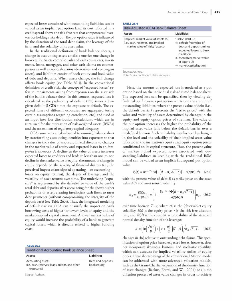
In the traditional defi nition of bank balance sheets, a change in accounting assets entails a one- for- one change in book equity. Assets comprise cash and cash equivalents, invest-ments, loans, mortgages, and other cash claims on counter-parties as well as noncash claims (derivatives and contingent assets), and liabilities consist of book equity and book value of debt and deposits. When assets change, the full change aff ects book equity (see Table 26.3). In the conventional defi nition of credit risk, the concept of “expected losses” re-fers to impairments arising from exposures on the asset side of the bank’s balance sheet. In this context, expected loss is calculated as the probability of default (PD) times a loss- given- default (LGD) times the exposure at default. Th e ex-pected losses of diff erent exposures are aggregated (using certain assumptions regarding correlation, etc.) and used as an input into loss distribution calculations, which are in turn used for the estimation of risk- weighted assets (RWAs) and the assessment of regulatory capital adequacy.
CCA constructs a risk- adjusted (economic) balance sheet by transforming accounting identities into exposures so that changes in the value of assets are linked directly to changes in the market value of equity and expected losses in an inte-grated framework. A decline in the value of assets increases expected losses to creditors and leads to less than one- to- one decline in the market value of equity; the amount of change in equity depends on the severity of fi nancial distress (i.e., the perceived impact of anticipated operating— or accounting— losses on equity returns), the degree of leverage, and the volatility of asset returns over time. Th e underlying “expo-sure” is represented by the default- free value of the bank’s total debt and deposits after accounting for the (now) higher probability of assets creating insuffi cient cash fl ows to meet debt payments (without compromising the integrity of the deposit base) (see Table 26.4). Th us, the integrated modeling of default risk via CCA can quantify the impact on bank borrowing costs of higher (or lower) levels of equity and the market- implied capital assessment. A lower market value of equity would increase the probability of a bank to generate capital losses, which is directly related to higher funding costs.
TABLE 26.3
Traditional Accounting Bank Balance SheetAssets Liabilities
Accounting assets Debt and deposits(i.e., cash, reserves, loans, credits, and other
exposures)Book equity
Source: Authors.
TABLE 26.4
Risk- Adjusted (CCA) Bank Balance SheetAssets Liabilities
(Implied) market value of assets (A) “Risky” debt (D)(i.e., cash, reserves, and implied
market value of “risky” assets)(= default- free value of
debt and deposits minus expected losses to bank creditors)
(Observable) market value of equity (E)
(= market capitalization)
Source: Authors.Note: CCA = contingent claims analysis.
536-57355_IMF_StressTestHBk_ch03_3P.indd 415 11/5/14 2:06 AM
Systemic Contingent Claims Analysis 416
sets and asset volatility, and assumptions about the default barrier) could fail to capture some relevant economics that are needed to fully understand default risk and thus could generate biased estimators of expected losses. Moreover, eq-uity prices might not only refl ect fundamental values be-cause of both shareholder dilution and trading behavior that obfuscate proper economic interpretation.16
Estimating the Joint Expected Losses from Default Risk
Second, the individually estimated expected losses are com-bined to determine the magnitude of default risk on a sys-temwide level. Th e distribution of expected losses is assumed to be “fat- tailed” in keeping with EVT. Th is specifi cation of individual loss estimates then informs the estimation of the dependence function. As part of a three- step subpro cess, we defi ne the univariate marginal density functions of all fi rms, which are then combined with their dependence function in order to generate an aggregate mea sure of default risk. Th is multivariate setup underpinning the Systemic CCA frame-work formally captures the realizations of joint expected losses. We can then use tail risk estimates, such as the conditional VaR (or expected shortfall, or ES), in order to gauge systemic solvency risk in times of stress.
1. Estimating the Marginal Distributions of Individual Expected Losses. We fi rst specify the statistical distribution of individual expected losses (based on the series of put op-tion values obtained for each fi rm) in accordance with EVT. Th is is a general statistical concept of deriving a limit law for sample maxima. Let the vector- valued series
Xmn = PE,1
i (t ),…,PE,mn (t ) (26.4)
denote in de pen dent, identically distributed random observa-tions of expected losses (i.e., a total of n- number of daily put option values PE,m
i (t ) up to time t), each estimated according to equation (26.1) over a rolling window of observations with periodic updating (e.g., a daily sliding window of 120 days) for j m fi rms in the sample. Th e individual asymptotic tail behavior is modeled in accordance with the Fisher- Tippett- Gnedenko theorem (Fisher and Tippett, 1928; Gnedenko, 1943), which defi nes the attribution of a given distribution of normalized maxima (or minima) to be of extremal type (as-suming that the underlying function is continuous on a closed interval). Given
Xn = max PE, j1 (t ),…,PE, j
n (t )( ), (26.5)
there exists a choice of normalizing constants n > 0 and n, such that the probability of each ordered n- sequence of nor-malized sample maxima (Xn– n)/ n converges to the nonde-generate limit distribution H(x) as n and x , so that
16 For instance, during the fi nancial crisis, rapid declines in market capital-ization of fi rms were not only a signal about future solvency risk but also refl ected a “fl ight to quality” motive that was largely unrelated to expec-tations about future fi rm earnings or profi tability.
more robust and reliable estimation results.12 Some of these approaches have been applied in the empirical use of the Sys-temic CCA framework in this chapter.13
Given that the asset value is infl uenced by the empirical irregularities contained in the Merton model (which also af-fects the model- based calibration of implied asset volatility), it is estimated directly from observable equity option prices.14 Th e state- price density (SPD) of the implied asset value is estimated from the risk- neutral probability distribution of the underlying asset price at the maturity date of equity op-tions with diff erent strike prices, without any assumptions on the underlying asset diff usion pro cess (which is assumed to be log- normal in the Merton model). Th e implied asset value is defi ned as the expectation over the empirical SPD by adapting the well- established Breeden and Litzenberger (1978) method, together with a semiparametric specifi cation of the Black- Scholes option pricing formula (Aït- Sahalia and Lo, 1998). More specifi cally, this approach uses the second derivative of the call pricing function (on Eu ro pe an options) with respect to the strike price (rather than option price). Estimates are based on option contracts with identical time to maturity, assuming a continuum of strike prices.15 Th e SPD of the equity price includes the risk- neutral expectation of the implied asset value and removes the impact of diff er-ences of higher moments of both the equity price and the implied asset value dynamics over the chosen time horizon. Th us, the current implied asset value can be transposed from the SPD of the equity price conditional on the contempora-neous leverage of the fi rm.
Note, however, that the presented valuation model is sub-ject to varying degrees of estimation uncertainty and paramet-ric assumptions. Th e option pricing model (given its specifi c distributional assumptions, the derivation of both implied as-
12 Th e suggested approach takes into account the nonlinear characteristics of asset price changes, which deviate from normality and are frequently infl uenced by stochastic volatility. Th e BSM model has been shown to consistently understate spreads ( Jones, Mason, and Rosenfeld, 1984; Ogden, 1987), with more recent studies pointing to considerable pric-ing errors because of its simplistic nature.
13 Other extensions are aimed at imposing more realistic assumptions, such as the introduction of stationary leverage ratios (Collin- Dufresne and Goldstein, 2001) and stochastic interest rates (Longstaff and Schwartz, 1995). Incorporating early default (Black and Cox, 1976) does not repre-sent a useful extension in this context given the short estimation and forecasting time window.
14 Given that the implied asset value is derived separately, this approach avoids the (problematic) “two- equations- two- unknowns” approach to de-rive implied assets and asset volatility based on Jones, Mason, and Rosen-feld (1984), which was subsequently extended by Ronn and Verma (1986) to a single equation to solve two simultaneous equations for asset value and volatility as two unknowns. Duan (1994) shows that the volatility relation between implied assets and equity could become redundant if the equity volatility is stochastic. An alternative estimation technique for asset volatility introduces a maximum likelihood approach (Erics-son and Reneby, 2004, 2005).
15 Because available strike prices always are discretely spaced on a fi nite range around the actual asset value, interpolation of the call pricing function inside this range and extrapolation outside this range are per-formed by means nonparametric (local polynomial) regression of the implied volatility surface (Rookley, 1997).
536-57355_IMF_StressTestHBk_ch03_3P.indd 416 11/5/14 2:06 AM
Andreas A. Jobst and Dale F. Gray 417
case and adjusting the margins according to Hall and Taj-vidi (2000) so that
( )=min 1, max n j=1m yi, j y
i j
ji=1
n1
, , 1 , (26.10)
where yi j = yi , j ni=1
n refl ects the average marginal density of all i n put option values and 0 max ( 1,…, m−1)
( j ) 1 for all 0 j 1.19 (i) represents a convex func-tion on [0,1] with (0) = (1) = 1, that is, the upper and lower limits of (i) are obtained under complete dependence and mutual in de pen dence, respectively. It is estimated iteratively (over a rolling window of observations with periodic up-dating at a frequency that is consistent with that in equation (26.5), subject to the optimization of the (m 1)-dimensional unit simplex:
Sm = ( 1,…, m 1) +
m: j 0,1 j m 1;
j 1 and m = 1 jj=1
m 1
j=1
m 1
, (26.11)
which establishes the degree of coincidence of multiple series of cross- classifi ed random variables similar to a chi- statistic that mea sures the statistical likelihood that observed values diff er from their expected distribution. Th is specifi cation stands in contrast to a general copula function that links the marginal distributions using only a single (and time- invariant) dependence pa ram e ter.
3. Estimating the Joint Distribution and a Tail Risk Mea-sure of Joint Expected Losses. We then combine the mar-ginal distributions of these individual expected losses with their dependence structure to generate a multivariate ex-treme value distribution over the same estimation period as earlier.20 Th e resultant cumulative distribution function is specifi ed as
Gt,m(x ) = exp yt, jj=1
m
t ( ) , (26.12)
19 Note that the marginal density of a given extreme relative to the average marginal density of all extremes is minimized (“ ”) across all fi rms j m, subject to the choice of factor j. A bivariate version of this ap-proach has been implemented in Jobst and Kamil (2008).
20 Th e analysis of dependence in this presented approach is completed separately from the analysis of marginal distributions and thus diff ers from the classical approach, where multivariate analysis is performed jointly for marginal distributions and their dependence structure by considering the complete variance– covariance matrix, using techniques like the Multivariate Generalized AutoRegressive Conditional Hetero-skedasticity approach. To obtain a multivariate distribution function, the dependence function combines several marginal distribution func-tions in accordance with Sklar’s (1959) theorem on constructing joint distributions with arbitrary marginal distributions via copula functions (which completely describes the dependence structure and contains all the information to link the marginal distributions). For the formal treatment of copulas and their properties, see Hutchinson and Lai (1990); Dall’Aglio, Kotz, and Salinetti (1991); and Joe (1997).
Fnnx+ n
(x ) = limn
PrXn n
ny
= F( ny + n )[ ]n H(x ) (26.6)
falls within the maximum domain of attraction (MDA) of the GEV as limiting distribution of maxima of dependent random variables (Coles, Heff ernan, and Tawn, 1999; Poon, Rockinger, and Tawn, 2003; Jobst, 2007) with the cumula-tive distribution function
H , , (x )=exp 1+ (x )
1/
if 1+ (x )0
exp expx
if x , = 0
(26.7)
and diff erencing equation (26.7) above as H , , (x) =ddx
H , , (x) yields the probability density function,
h , , (x ) =1
1+(x )
( 1/ ) 1
exp 1+(x )
+
1/
. (26.8)
Th us, the jth univariate marginal density function of each expected loss series converging to GEV in the limit is de-fi ned as
y j (x ) = 1+ ˆj
(x ˆ j )ˆ j
+
1/ j
(for j = 1,…, m) (26.9)
where 1 + j (x j)/ j > 0, scale pa ram e ter j > 0, location pa-ram e ter j , and shape pa ram e ter i 0.17 Th ese moments are estimated concurrently by means of numerical iteration via maximum likelihood (ML), which identifi es possible limiting laws of asymptotic tail behavior, that is, the likeli-hood of even larger extremes as the level of statistical confi -dence approaches certainty. Th e ML estimator in the GEV model is evaluated numerically by using an iteration proce-dure (e.g., over a rolling window of observations with peri-odic updating) to maximize the likelihood h , , (x | )i=1
n over all three pa ram e ters = ( , , ) simultaneously, where the linear combinations of ratios of spacings estimator serves as an initial value ( Jobst, 2014).18
2. Estimating the Dependence Structure of Individual Expected Losses. Second, we defi ne a nonparametric, multi-variate dependence function between the marginal distribu-tions of expected losses by expanding the bivariate logistic method proposed by Pickands (1981) to the multivariate
17 Th e upper tails of most (conventional) limit distributions (weakly) con-verge to this parametric specifi cation of asymptotic behavior, irrespec-tive of the original distribution of observed maxima (unlike parametric VaR models).
18 Note that the ML estimator fails for 1 since the likelihood function does not have a global maximum in this case. However, a local maximum close to the initial value can be attained.
536-57355_IMF_StressTestHBk_ch03_3P.indd 417 11/5/14 2:06 AM
Systemic Contingent Claims Analysis 418
where the relative weight of institution j is defi ned as the marginal contribution,
,m, a =
2Gt, ,m1 (a)
yt, j t ( )
s.t. , j, aj
m
=1 and , j, a z , j z ,m ,
(26.19)
attributable to the joint eff ect of both the marginal density and the change of the dependence function owing to the presence of institution j m in the sample.
2. EXTENSIONS OF THE SYSTEMIC CCA FRAMEWORK
A. Integrated market- implied capital assessment using CCA and Systemic CCA
Given that the evaluation of default risk is inherently linked to perceived riskiness as implied by the changes in equity and equity option prices, the risk- adjusted (economic) balance sheet approach— and its multivariate extension in the form of Systemic CCA— provides an integrated analytical frame-work for a market- based assessment of individual and sys-temwide solvency. Higher expected losses to creditors lead to less than a one- to- one decline in the market value of equity, depending on the severity of the perceived (and actual) de-cline in the value of assets, the degree of leverage, and the vola-tility of assets. Th us, the interaction between these constituent elements of the risk- adjusted (economic) balance sheet gives rise to a market- based capital assessment, which links changes in the value of assets directly to the market value of equity.
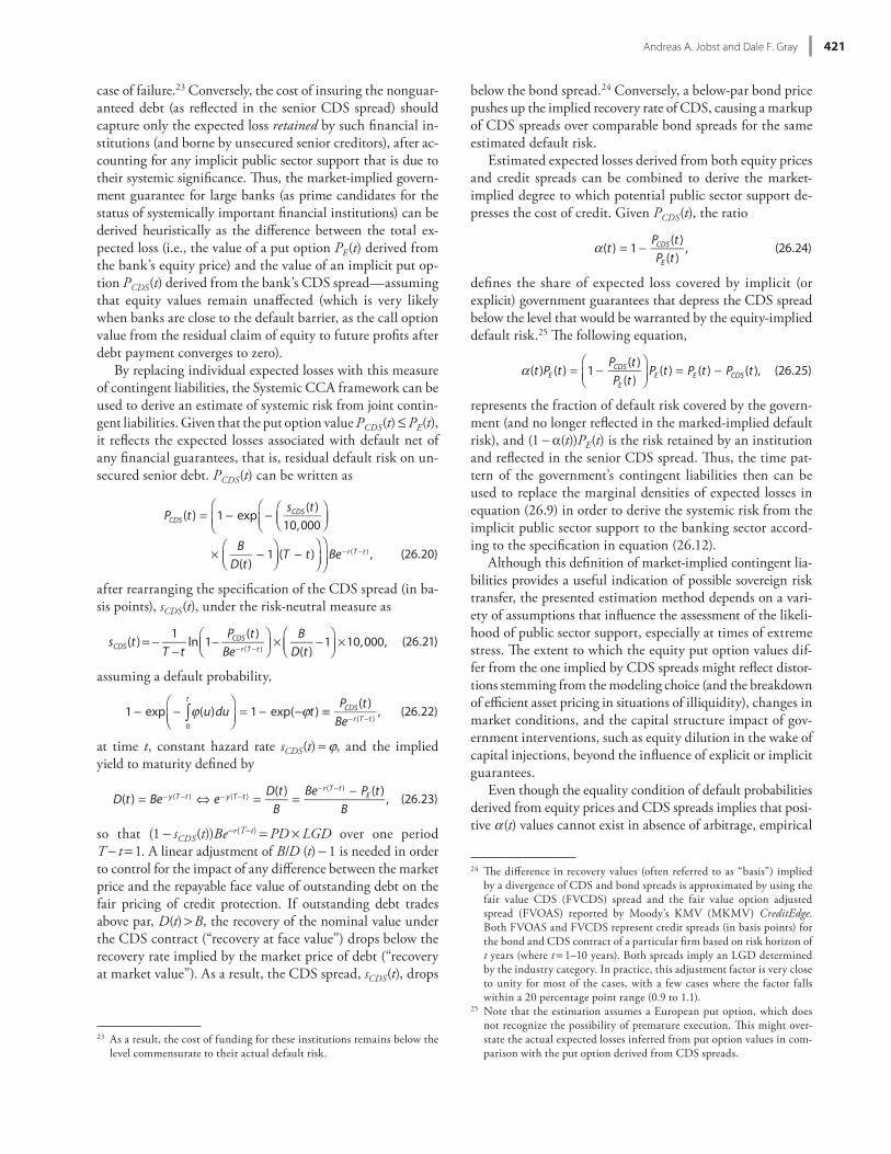
As opposed to the regulatory defi nition of capitalization (based on the discrete nature of accounting identities), the CCA- based capital assessment hinges on the historical dynam-ics of implied asset values and their eff ect on the magnitude of expected losses. Two broad indicators serve to illustrate this point: (1) the market- implied capital adequacy ratio (MCAR), which is defi ned as the ratio between the amount of market capitalization divided by the implied asset value of a fi rm; and (2) the expected loss ratio (“EL ratio”) between individual expected losses (at a defi ned percentile of statistical confi -dence) and the amount of market capitalization (see Figure 26.1, fi rst panel). Both ratios also can be generated on a sys-temwide basis, with inputs defi ned as sample aggregates of input variables to the multivariate specifi cation of the Sys-temic CCA. In this case, the EL ratio is defi ned by magnitude of joint expected losses (at the 95th percentile, for instance) relative to aggregate market capitalization of all sample fi rms (see Figure 26.1, second panel).
Th e market- implied capital assessment also can help iden-tify a capital shortfall. Th e MCAR represents an important analogue to the regulatory defi nition of capital adequacy, which refl ects the market’s perception of solvency (based on the implied value of assets relative to the prevailing default risk) and is completely removed from prudential determi-nants of default risk aff ecting a bank’s capital assessment,
with corresponding probability density function
(26.13)
at time t = + 1 by maximizing the likelihood gt,m(x | )j =1m
over all three pa ram e ters = ( , , ) simultaneously so that the ML estimate of the true values 0 is
ˆMLE = arg maxˆ( | x ) 0 . (26.14)
Finally, we obtain the joint ES (or conditional VaR) as a mea sure of CTE. ES defi nes the probability- weighted residual density (i.e., the average aggregate expected losses) beyond a prespecifi ed statistical confi dence level (“severity threshold”) over a given estimation time period. Given the dependence structure defi ned in equation (26.10), we can calculate ES in a multivariate context as
ESt, ,m, a = E z | z Gt, ,m1 (a) = VaRt, a , (26.15)
where G 1(a) is the quantile corresponding to probability 0 < a < 1 (say, a = 0.95), z and G 1(a) = G (a) with G (a)
inf (x|G(x a)) so that
VaRt, a = sup Gt, ,m1 (a) |Pr[z > Gt, ,m
1 (a)] a = 0.95{ }, (26.16)
with the point estimate of joint potential losses of m fi rms at time t defi ned as
Gt, ,m1 (a)= ˆ t,m + ˆ t,m / ˆ
t,m
ln(a)
t ( )
ˆt,m
1 . (26.17)
Th e contribution of each fi rm can be determined by calcu-lating the cross- partial derivative of the joint distribution of expected losses. Th e joint ES also can be written as a linear combination of individual ES values, ESt, , j,a, where the rela-tive weights , m, a (in the weighted sum) are given by the second order cross- partial derivative of the inverse of the joint probability density function Gt, ,m
1 (i) to changes in both the dependence function t (i) and the individual marginal severity yi, j of expected losses. Th us, the contribution can be derived as the partial derivative of the multivariate density to changes in the relative weight of the univariate marginal distri-bution of expected losses and its impact on the dependence function (of all expected losses of sample fi rms) at the specifi ed percentile. By rewriting ESt, ,m,a, in equation (26.15), we ob-tain the following:
ESt, ,m, a = ,m, aj
m
E z , j | z ,m Gt, ,m1 (a)=VaRt, a , (26.18)
21 ES is an improvement over VaR, which, in addition to being a pure fre-quency mea sure, is “incoherent,” that is, it violates several axioms of monotonicity, subadditivity, positive homogeneity, and translation in-variance found in coherent risk mea sures. For the application of this kind of coherent risk mea sure, we refer to Artzner and others (1999) as well as Wirch and Hardy (1999).
exp yt , jj=1
m
t ( ) ,
gt ,m(x )= 1ˆ t ,m
yt , jj=1
m
t ( )
1
536-57355_IMF_StressTestHBk_ch03_3P.indd 418 11/5/14 2:06 AM
Andreas A. Jobst and Dale F. Gray 419
MCAR =Market Capitalization/Implied
AssetsFair Value Credit
Spread
EL R
atio
=Ex
pect
ed L
osse
s (fr
om C
CA)/
Mar
ket C
apita
lizat
ion
Impl
ied
Asse
tVo
latil
ity
IndividualRisk
Assessment
Source: Authors.Note: CAR = capital adequacy ratio; CCA = contingent claims analysis; EL = expected losses; MCAR = market- implied CAR.
Figure 26.1 Integrated Market- Based Capital Assessment Using CCA and Systemic CCA (based on nonlinear relation between CCA- based CAR, EL ratio, fair value credit spread, and implied asset volatility)
Systemic RiskAssessment
Aggregate MCAR =Aggregate Market Capitalization/
Aggregate Implied Assets
Joi
nt E
L Ra
tio =
Join
t Exp
ecte
d Lo
sses
(fro
mSy
stem
ic C
CA)/A
ggre
gate
Mar
ket C
apita
lizat
ion
Impl
ied
Asse
tVo
latil
ity(s
ampl
e m
edia
n)
Aggregate Fair Value CreditSpread
536-57355_IMF_StressTestHBk_ch03_3P.indd 419 11/5/14 2:06 AM
Systemic Contingent Claims Analysis 420
cial institutions (and large banks in par tic u lar) but also raises default risk in the fi nancial sector overall (which increases the cost of borrowing). Th ere is also a higher likelihood of down-grades to fi nancial institutions following downgrades of sov-ereign credit ratings, which establish an upper ceiling to their unsecured funding ratings. Th is linkage between the credit-worthiness of the sovereign and the fi nancial system (in par-tic u lar, the banking sector) is prone to perpetuate a negative feedback eff ect that is accentuated by the lender– borrower channel in situations where fi nancial institutions hold large exposures to public sector entities.
Based on CCA, the market- implied expected losses calcu-lated from equity market and balance sheet information of fi -nancial institutions can be combined with information from their credit default swap (CDS) contracts to estimate the gov-ernment’s contingent liabilities.22 Because systemically impor-tant institutions enjoy an implicit government guarantee, their creditors have an expectation of public sector support in the
22 See Gray and Jobst (2009b). See also Gapen (2009) for an application on CCA to the mea sure ment of contingent liabilities from government- sponsored enterprises in the United States.
such as risk- weighted assets. In the empirical section of the chapter, the relation between the MCAR and regulatory capi-tal adequacy is investigated further, which establishes the pos-sibility of defi ning a systemically based capital shortfall using CCA- based mea sures of solvency (see Section 3).
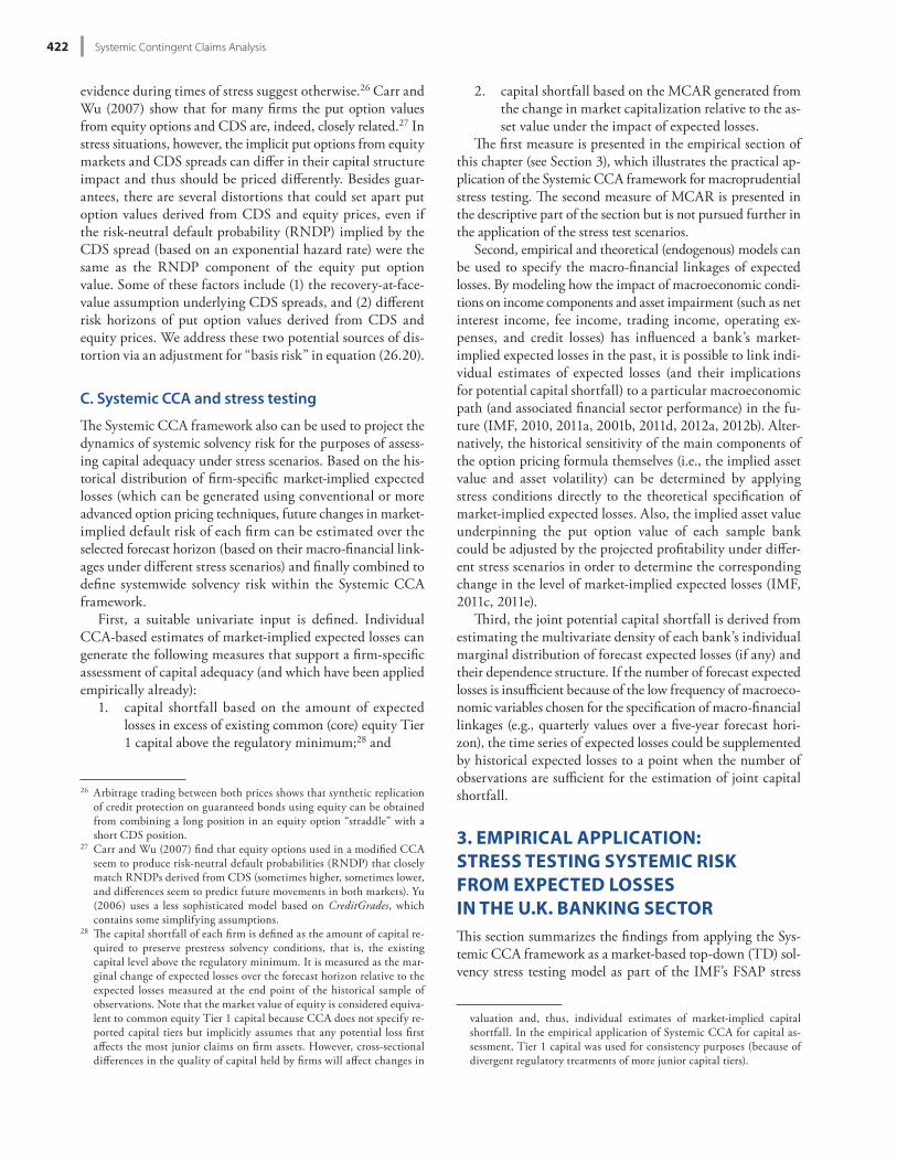
B. Estimating the contingent liabilities to the public sector
Large implicit government fi nancial guarantees (valued as contingent liabilities) create signifi cant valuation linkages between sovereigns and fi nancial sector risks. Th ese linkages could give rise to a destabilization pro cess that increases the susceptibility of public fi nances to the potential impact of distress in an outsized fi nancial sector (see Figure 26.2). Th e fi nancial crisis that started in 2007 is a stark reminder of how public sector support mea sures provided to large fi nancial in-stitutions can result in considerable risk transfer to the gov-ernment, which places even greater emphasis on long- term fi scal sustainability. A negative feedback loop between the fi nancial sector risks and fi scal policy arises because a decline in the market value of sovereign debt not only weakens the implicit sovereign guarantees to systemically important fi nan-
Sovereign Banks
ForeignSovereign
ForeignBanks
1. Lower marked-to-market (MTM) in value ofall government bonds held by local banks
2. Increase in bank funding costs3. Erosion in potential for official
support/bailout
Increase in contingent liabilities
Similar sovereignscome under
pressureRise in counterparty
credit risk
Lower marked-to-market (MTM) invalue of all government bonds
held by foreign banks
Increase in contingent liabilities
Dom
estic
eco
nom
yFo
reig
n ec
onom
y
Source: Authors.
Figure 26.2 Valuation Linkages between the Sovereign and Banking Sector
536-57355_IMF_StressTestHBk_ch03_3P.indd 420 11/5/14 2:06 AM
Andreas A. Jobst and Dale F. Gray 421
below the bond spread.24 Conversely, a below- par bond price pushes up the implied recovery rate of CDS, causing a markup of CDS spreads over comparable bond spreads for the same estimated default risk.
Estimated expected losses derived from both equity prices and credit spreads can be combined to derive the market- implied degree to which potential public sector support de-presses the cost of credit. Given PCDS(t), the ratio
(t ) = 1PCDS (t )PE (t )
, (26.24)
defi nes the share of expected loss covered by implicit (or explicit) government guarantees that depress the CDS spread below the level that would be warranted by the equity- implied default risk.25 Th e following equation,
(t )PE (t ) = 1PCDS (t )PE (t )
PE (t ) = PE (t ) PCDS (t ), (26.25)
represents the fraction of default risk covered by the govern-ment (and no longer refl ected in the marked- implied default risk), and (1 (t))PE(t) is the risk retained by an institution and refl ected in the se nior CDS spread. Th us, the time pat-tern of the government’s contingent liabilities then can be used to replace the marginal densities of expected losses in equation (26.9) in order to derive the systemic risk from the implicit public sector support to the banking sector accord-ing to the specifi cation in equation (26.12).
Although this defi nition of market- implied contingent lia-bilities provides a useful indication of possible sovereign risk transfer, the presented estimation method depends on a vari-ety of assumptions that infl uence the assessment of the likeli-hood of public sector support, especially at times of extreme stress. Th e extent to which the equity put option values dif-fer from the one implied by CDS spreads might refl ect distor-tions stemming from the modeling choice (and the breakdown of effi cient asset pricing in situations of illiquidity), changes in market conditions, and the capital structure impact of gov-ernment interventions, such as equity dilution in the wake of capital injections, beyond the infl uence of explicit or implicit guarantees.
Even though the equality condition of default probabilities derived from equity prices and CDS spreads implies that posi-tive (t) values cannot exist in absence of arbitrage, empirical
24 Th e diff erence in recovery values (often referred to as “basis”) implied by a divergence of CDS and bond spreads is approximated by using the fair value CDS (FVCDS) spread and the fair value option adjusted spread (FVOAS) reported by Moody’s KMV (MKMV) CreditEdge. Both FVOAS and FVCDS represent credit spreads (in basis points) for the bond and CDS contract of a par tic u lar fi rm based on risk horizon of t years (where t = 1– 10 years). Both spreads imply an LGD determined by the industry category. In practice, this adjustment factor is very close to unity for most of the cases, with a few cases where the factor falls within a 20 percentage point range (0.9 to 1.1).
25 Note that the estimation assumes a Eu ro pe an put option, which does not recognize the possibility of premature execution. Th is might over-state the actual expected losses inferred from put option values in com-parison with the put option derived from CDS spreads.
case of failure.23 Conversely, the cost of insuring the nonguar-anteed debt (as refl ected in the se nior CDS spread) should capture only the expected loss retained by such fi nancial in-stitutions (and borne by unsecured se nior creditors), after ac-counting for any implicit public sector support that is due to their systemic signifi cance. Th us, the market- implied govern-ment guarantee for large banks (as prime candidates for the status of systemically important fi nancial institutions) can be derived heuristically as the diff erence between the total ex-pected loss (i.e., the value of a put option PE(t) derived from the bank’s equity price) and the value of an implicit put op-tion PCDS(t) derived from the bank’s CDS spread— assuming that equity values remain unaff ected (which is very likely when banks are close to the default barrier, as the call option value from the residual claim of equity to future profi ts after debt payment converges to zero).
By replacing individual expected losses with this mea sure of contingent liabilities, the Systemic CCA framework can be used to derive an estimate of systemic risk from joint contin-gent liabilities. Given that the put option value PCDS(t) PE(t), it refl ects the expected losses associated with default net of any fi nancial guarantees, that is, residual default risk on un-secured se nior debt. PCDS(t) can be written as
PCDS (t ) = 1 expsCDS (t )10,000
BD(t )
1 (T t ) Be r (T t ) , (26.20)
after rearranging the specifi cation of the CDS spread (in ba-sis points), sCDS(t), under the risk- neutral mea sure as
sCDS (t )=1
T tln 1
PCDS (t )Be r (T t )
BD(t )
1 10,000, (26.21)
assuming a default probability,
1 exp (u)du0
t
= 1 exp( t )PCDS (t )Be r (T t )
, (26.22)
at time t, constant hazard rate sCDS(t) , and the implied yield to maturity defi ned by
D(t ) = Be y (T t ) e y (T t ) = D(t )B
= Be r (T t ) PE (t )B
, (26.23)
so that (1 sCDS(t))Be r(T t) = PD × LGD over one period T t = 1. A linear adjustment of B/D (t) 1 is needed in order to control for the impact of any diff erence between the market price and the repayable face value of outstanding debt on the fair pricing of credit protection. If outstanding debt trades above par, D(t) > B, the recovery of the nominal value under the CDS contract (“recovery at face value”) drops below the recovery rate implied by the market price of debt (“recovery at market value”). As a result, the CDS spread, sCDS(t), drops
23 As a result, the cost of funding for these institutions remains below the level commensurate to their actual default risk.
536-57355_IMF_StressTestHBk_ch03_3P.indd 421 11/5/14 2:06 AM
Systemic Contingent Claims Analysis 422
2. capital shortfall based on the MCAR generated from the change in market capitalization relative to the as-set value under the impact of expected losses.
Th e fi rst mea sure is presented in the empirical section of this chapter (see Section 3), which illustrates the practical ap-plication of the Systemic CCA framework for macroprudential stress testing. Th e second mea sure of MCAR is presented in the descriptive part of the section but is not pursued further in the application of the stress test scenarios.
Second, empirical and theoretical (endogenous) models can be used to specify the macro- fi nancial linkages of expected losses. By modeling how the impact of macroeconomic condi-tions on income components and asset impairment (such as net interest income, fee income, trading income, operating ex-penses, and credit losses) has infl uenced a bank’s market- implied expected losses in the past, it is possible to link indi-vidual estimates of expected losses (and their implications for potential capital shortfall) to a par tic u lar macroeconomic path (and associated fi nancial sector per for mance) in the fu-ture (IMF, 2010, 2011a, 2001b, 2011d, 2012a, 2012b). Alter-natively, the historical sensitivity of the main components of the option pricing formula themselves (i.e., the implied asset value and asset volatility) can be determined by applying stress conditions directly to the theoretical specifi cation of market- implied expected losses. Also, the implied asset value underpinning the put option value of each sample bank could be adjusted by the projected profi tability under diff er-ent stress scenarios in order to determine the corresponding change in the level of market- implied expected losses (IMF, 2011c, 2011e).
Th ird, the joint potential capital shortfall is derived from estimating the multivariate density of each bank’s individual marginal distribution of forecast expected losses (if any) and their dependence structure. If the number of forecast expected losses is insuffi cient because of the low frequency of macroeco-nomic variables chosen for the specifi cation of macro- fi nancial linkages (e.g., quarterly values over a fi ve- year forecast hori-zon), the time series of expected losses could be supplemented by historical expected losses to a point when the number of observations are suffi cient for the estimation of joint capital shortfall.
3. EMPIRICAL APPLICATION: STRESS TESTING SYSTEMIC RISK FROM EXPECTED LOSSES IN THE U.K. BANKING SECTORTh is section summarizes the fi ndings from applying the Sys-temic CCA framework as a market- based top- down (TD) sol-vency stress testing model as part of the IMF’s FSAP stress
valuation and, thus, individual estimates of market- implied capital shortfall. In the empirical application of Systemic CCA for capital as-sessment, Tier 1 capital was used for consistency purposes (because of divergent regulatory treatments of more ju nior capital tiers).
evidence during times of stress suggest otherwise.26 Carr and Wu (2007) show that for many fi rms the put option values from equity options and CDS are, indeed, closely related.27 In stress situations, however, the implicit put options from equity markets and CDS spreads can diff er in their capital structure impact and thus should be priced diff erently. Besides guar-antees, there are several distortions that could set apart put option values derived from CDS and equity prices, even if the risk- neutral default probability (RNDP) implied by the CDS spread (based on an exponential hazard rate) were the same as the RNDP component of the equity put option value. Some of these factors include (1) the recovery- at- face- value assumption underlying CDS spreads, and (2) diff erent risk horizons of put option values derived from CDS and equity prices. We address these two potential sources of dis-tortion via an adjustment for “basis risk” in equation (26.20).
C. Systemic CCA and stress testing
Th e Systemic CCA framework also can be used to project the dynamics of systemic solvency risk for the purposes of assess-ing capital adequacy under stress scenarios. Based on the his-torical distribution of fi rm- specifi c market- implied expected losses (which can be generated using conventional or more advanced option pricing techniques, future changes in market- implied default risk of each fi rm can be estimated over the selected forecast horizon (based on their macro- fi nancial link-ages under diff erent stress scenarios) and fi nally combined to defi ne systemwide solvency risk within the Systemic CCA framework.
First, a suitable univariate input is defi ned. Individual CCA- based estimates of market- implied expected losses can generate the following mea sures that support a fi rm- specifi c assessment of capital adequacy (and which have been applied empirically already):
1. capital shortfall based on the amount of expected losses in excess of existing common (core) equity Tier 1 capital above the regulatory minimum;28 and
26 Arbitrage trading between both prices shows that synthetic replication of credit protection on guaranteed bonds using equity can be obtained from combining a long position in an equity option “straddle” with a short CDS position.
27 Carr and Wu (2007) fi nd that equity options used in a modifi ed CCA seem to produce risk- neutral default probabilities (RNDP) that closely match RNDPs derived from CDS (sometimes higher, sometimes lower, and diff erences seem to predict future movements in both markets). Yu (2006) uses a less sophisticated model based on CreditGrades, which contains some simplifying assumptions.
28 Th e capital shortfall of each fi rm is defi ned as the amount of capital re-quired to preserve prestress solvency conditions, that is, the existing capital level above the regulatory minimum. It is mea sured as the mar-ginal change of expected losses over the forecast horizon relative to the expected losses mea sured at the end point of the historical sample of observations. Note that the market value of equity is considered equiva-lent to common equity Tier 1 capital because CCA does not specify re-ported capital tiers but implicitly assumes that any potential loss fi rst aff ects the most ju nior claims on fi rm assets. However, cross- sectional diff erences in the quality of capital held by fi rms will aff ect changes in
536-57355_IMF_StressTestHBk_ch03_3P.indd 422 11/5/14 2:06 AM
Andreas A. Jobst and Dale F. Gray 423
VaR values of individual expected losses or the joint 95 per-cent ES divided by the aggregate market capitalization) and the aggregate MCAR. Th e empirical results suggested an even higher sensitivity of MCAR to changes in systemwide expected losses than in the case of the single- fi rm example shown in Figure 26.3. In addition, the comparison of MCAR to the regulatory benchmark (Core Tier 1) indicates that the improvement of solvency conditions after the peak of the fi -nancial crisis in March 2009 appeared more protracted across all sample fi rms (see Figure 26.4, bottom chart).
B. Estimating expected losses under stress conditions based on macro- fi nancial linkages
Individual market- implied expected losses under stress condi-tions were derived from their historical sensitivity to changes in macro- fi nancial conditions and bank per for mance. Expected losses under diff erent stress scenarios were forecast using two diff erent methods for the specifi cation of the macro- fi nancial linkages of expected losses as mea sured by the implicit put option values of sample fi rms (see Section 2.B):
• In the fi rst model (“IMF satellite model”), expected losses were estimated using a dynamic panel regres-sion specifi cation with several macroeconomic vari-ables (short- term interest rate [+], long- term interest rate [ ], real GDP [ ], and unemployment [+]) and several bank- specifi c output variables (net interest income [+], operating profi t before taxes [ ], credit losses [+], leverage [+], and funding gap [+]).31
• In the second model (“structural model”), the value of implied assets of each bank as at end- 2010 is ad-justed by forecasts of operating profi t and credit losses generated in the Bank of En gland’s Risk As-sessment Model for Systemic Institutions (RAMSI) in order to derive a revised put option value (after reestimating implied asset volatility), which deter-mines the market- implied capital loss.32
Th e individually estimated expected losses then were trans-posed into a capital shortfall. Th e potential capital loss was determined on an individual basis as the marginal change of expected losses over the forecast horizon (2011– 2015) and evaluated for each macro- fi nancial approach and under each of the specifi ed adverse scenarios. As an alternative, the market- implied CAR (see Figures 26.3 and 26.4) could have been used as a basis for assessing capital adequacy and the extent to which expected losses result in potential capital shortfall. However, in the context of this exercise, the CCA- based results were transposed into conventional (regulatory)
31 Th e plus or minus signs indicate whether the selected variable exhibited a positive or negative regression coeffi cient. To be included in the model, the variables needed to be statistically signifi cant at least at the 10 per-cent level.
32 Th is approach also assumed a graduated increase of the default barrier consistent with the transition period to higher capital requirements for the most ju nior levels of equity under Basel III standards (Basel Com-mittee on Banking Supervision, 2012).
test of the U.K. banking sector (IMF, 2011e).29 Th e model was estimated based on market and balance sheet informa-tion of the fi ve largest commercial banks, the largest build-ing society, and the largest foreign retail bank using daily data between January 3, 2005, and end- March 2011.30 Th e individual market- implied expected losses were treated as a portfolio, whose combined default risk over a prespecifi ed time horizon generated estimates of individual fi rms’ contri-butions to systemic risk in the event of distress (“tail risk”).
A. Illustrating the nonlinearity of historical estimates of individual and joint expected losses
Based on the historical estimates of expected losses, the risk- based valuation of default risk within the Systemic CCA framework supports an integrated market- based capital as-sessment (see Section 2). Figure 26.3 illustrates the nonlin-ear relation between the daily estimates of the MCAR, the EL ratio, the fair value credit spread, and the implied asset volatility of one selected sample fi rm in accordance with the stylized example shown in Figure 26.1. As expected, the ris-ing default risk during the fi nancial crisis establishes a high sensitivity of MCAR to a precipitous increase of expected losses at a level consistent with the regulatory mea sure of capital adequacy (see Figure 26.3, second panel). However, the growing gap between MCAR and the Core Tier 1 ratio toward the end point of the estimation time period implies that capitalization of the selected bank was perceived by in-vestors as much lower than what regulatory standards would otherwise suggest.
Similarly, the interaction between these variables also can be shown on a systemwide basis (see Figure 26.4). For all fi rms in the sample, the fi rm- specifi c variables underpinning the presented mea sure were replaced with systemwide mea sures, such as the joint EL ratio (defi ned as the sum of 95 percent
29 Th e Systemic CCA framework also served as a means of cross- validating the stress testing results from the bottom- up exercise conducted jointly with the Financial Ser vices Authority (FSA).
30 Th e sample comprised the following fi rms: Hongkong and Shanghai Banking Corporation (HSBC), Barclays, Royal Bank of Scotland (RBS), Lloyds’s Banking Group, Standard Chartered Bank, Nationwide, and Santander U.K. Key inputs used were the daily implied asset values de-rived as the expectation over the state- price density (SPD) using equity option data (from Bloomberg), the default barrier estimated for each fi rm based on quarterly fi nancial accounts (from MKMV CreditEdge), the risk- free rate of interest (r = 3.0 percent), a one- year time horizon T = 1, and one- year CDS spreads on se nior debt (from MarkIt). Th e de-fault barrier was set equal to total short- term debt plus one- half of long- term debt, consistent with the approach taken by MKMV CreditEdge. More specifi cally, the SPD is calculated using daily European- style eq-uity call option price data over the sample time period with a time to maturity of three months. Besides the maturity tenor, option price data also included information on strike prices as well as actual and cor-rected spot prices (with implied dividends taken into account). Th e multivariate distribution of expected losses (i.e., the implicit put option value over a one- year horizon) across all sample fi rms was estimated over a rolling window of 60 working days (i.e., three months) with daily up-dating, consistent with the maturity tenor of equity option prices used for the estimation of the implied asset value of each fi rm.
536-57355_IMF_StressTestHBk_ch03_3P.indd 423 11/5/14 2:06 AM
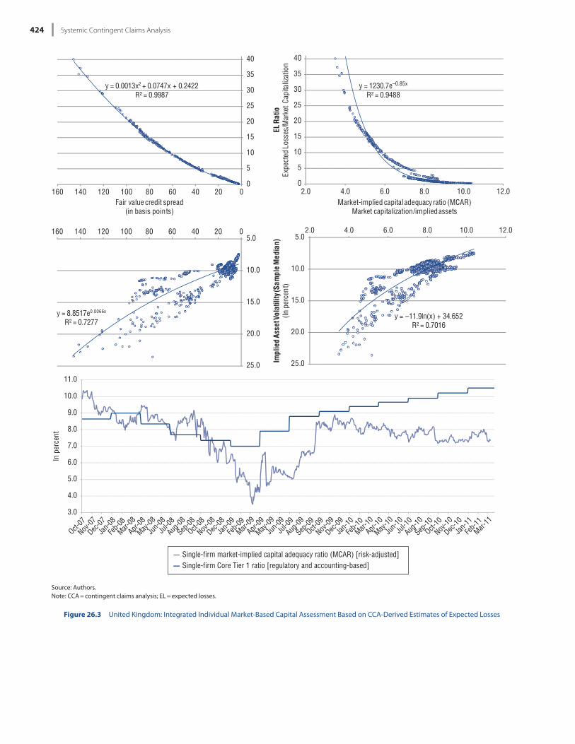
Systemic Contingent Claims Analysis 424
y = 0.0013x2 + 0.0747x + 0.2422R² = 0.9987
0
5
10
15
20
25
30
35
40
020406080100120140160
EL R
atio
Expe
cted
Los
ses/
Mar
ket C
apita
lizat
ion
Fair value credit spread(in basis points)
y = 1230.7e–0.85x
R² = 0.9488
0
5
10
15
20
25
30
35
40
2.0 4.0 6.0 8.0 10.0 12.0Market-implied capital adequacy ratio (MCAR)
Market capitalization/implied assets
y = 8.8517e0.0066x
R² = 0.7277
5.0
10.0
15.0
20.0
25.0
020406080100120140160
Impl
ied
Asse
t Vol
atili
ty (S
ampl
e M
edia
n)(In
per
cent
)
y = –11.9ln(x) + 34.652R² = 0.7016
5.0
10.0
15.0
20.0
25.0
2.0 4.0 6.0 8.0 10.0 12.0
3.0
4.0
5.0
6.0
7.0
8.0
9.0
10.0
11.0
Oct-07
Nov-07
Dec-07
Jan-0
8
Feb-0
8
Mar-08
Apr-08
May-08
Jun-0
8
Jul-0
8
Aug-08
Sep-08
Oct-08
Nov-08
Dec-08
Jan-0
9
Feb-0
9
Mar-09
Apr-09
May-09
Jun-0
9
Jul-0
9
Aug-09
Sep-09
Oct-09
Nov-09
Dec-09
Jan-1
0
Feb-1
0
Mar-10
Apr-10
May-10
Jun-1
0
Jul-1
0
Aug-10
Sep-10
Oct-10
Nov-10
Dec-10
Jan-1
1
Feb-1
1
Mar-11
In p
erce
nt
Single-firm market-implied capital adequacy ratio (MCAR) [risk-adjusted]Single-firm Core Tier 1 ratio [regulatory and accounting-based]
Source: Authors.Note: CCA = contingent claims analysis; EL = expected losses.
Figure 26.3 United Kingdom: Integrated Individual Market- Based Capital Assessment Based on CCA- Derived Estimates of Expected Losses
536-57355_IMF_StressTestHBk_ch03_3P.indd 424 11/5/14 2:06 AM
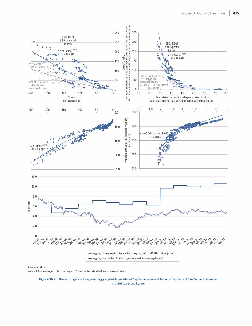
Andreas A. Jobst and Dale F. Gray 425
y = 0.1397x1.3212
R² = 0.8908
y = 0.098x1.2709
R² = 0.7964
0
50
100
150
200
250
300
050100150200250
Join
t EL
ratio
Join
t exp
ecte
d lo
sses
(95%
ES)
/agg
rega
te m
arke
t cap
italiz
atio
n [b
lack
circ
les]
Sum
of i
ndiv
idua
l exp
ecte
d lo
sses
(95%
VaR
)/mar
ket c
apita
lizat
ion
[red
circ
les]
Spread(in basis points)
Sum of 95% VaRof individual
expected losses
95% ES ofjoint expected
losses
y = 3223.3e–1.295x
R² = 0.9306
y = 4.4627x2 – 54.196x + 162.56R² = 0.92620
50
100
150
200
250
300
0.0 1.0 2.0 3.0 4.0 5.0 6.0 7.0 8.0Market-implied capital adequacy ratio (MCAR)
Aggregate market capitalization/aggregate implied assets
Sum of 95% VaRof individual
expected losses
95% ES ofjoint expected
losses
y = 8.8028e0.0038x
R² = 0.8937
5.0
10.0
15.0
20.0
25.0
050100150200250
Impl
ied
asse
t vol
atili
ty (s
ampl
e m
edia
n)(in
per
cent
) y = –8.301ln(x) + 22.843R² = 0.8383
5.0
10.0
15.0
20.0
25.0
0.0 1.0 2.0 3.0 4.0 5.0 6.0 7.0 8.0
0.0
2.0
4.0
6.0
8.0
10.0
12.0
Oct-07
Nov-07
Dec-07
Jan-0
8
Feb-0
8
Mar-08
Apr-08
May-08
Jun-0
8
Jul-0
8
Aug-08
Sep-08
Oct-08
Nov-08
Dec-08
Jan-0
9
Feb-0
9
Mar-09
Apr-09
May-09
Jun-0
9
Jul-0
9
Aug-09
Sep-09
Oct-09
Nov-09
Dec-09
Jan-1
0
Feb-1
0
Mar-10
Apr-10
May-10
Jun-1
0
Jul-1
0
Aug-10
Sep-10
Oct-10
Nov-10
Dec-10
Jan-1
1
Feb-1
1
Mar-11
In p
erce
nt
Aggregate market-implied capital adequacy ratio (MCAR) [risk-adjusted]
Aggregate core tier 1 ratio [regulatory and accounting-based]
Source: Authors.Note: CCA = contingent claims analysis; ES = expected shortfall; VaR = value at risk.
Figure 26.4 United Kingdom: Integrated Aggregate Market- Based Capital Assessment Based on Systemic CCA- Derived Estimates of Joint Expected Losses
536-57355_IMF_StressTestHBk_ch03_3P.indd 425 11/5/14 2:06 AM
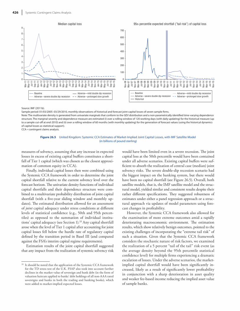
Systemic Contingent Claims Analysis 426
would have been limited even in a severe recession. Th e joint capital loss at the 50th percentile would have been contained under all adverse scenarios. Existing capital buff ers were suf-fi cient to absorb the realization of central case (median) joint solvency risks. Th e severe double- dip recession scenario had the biggest impact on the banking system, but there would have been no capital shortfall (see Figure 26.5). Overall, both satellite models, that is, the IMF satellite model and the struc-tural model, yielded similar and consistent results despite their rather diff erent specifi cations. Th ey suggested robustness of estimates under either a panel regression approach or a struc-tural approach via updates of model pa ram e ters using fore-cast changes in profi tability.
However, the Systemic CCA framework also allowed for the examination of more extreme outcomes amid a rapidly deteriorating macroeconomic environment. Th e estimation results, which show relatively benign outcomes, pointed to the existing challenges of incorporating the “extreme tail risk” of such a situation. Given that the Systemic CCA framework considers the stochastic nature of risk factors, we examined the realization of a 5 percent “tail of the tail” risk event (as the average density beyond the 95th percentile statistical confi dence level) for multiple fi rms experiencing a dramatic escalation of losses. Under the adverse scenarios, the market- implied capital shortfall would have been signifi cantly in-creased, likely as a result of signifi cantly lower profi tability in conjunction with a sharp deterioration in asset quality and weaker fee- based income reducing the implied asset value of sample banks.
mea sures of solvency, assuming that any increase in expected losses in excess of existing capital buff ers constitutes a short-fall of Tier 1 capital (which was chosen as the closest approxi-mation of common equity in CCA).
Finally, individual capital losses then were combined using the Systemic CCA framework in order to determine the joint capital shortfall relative to the current solvency level over the forecast horizon. Th e univariate density functions of individual capital shortfalls and their dependence structure were com-bined to a multivariate probability distribution of joint capital shortfall (with a fi ve- year sliding window and monthly up-dates). Th e estimated distribution allowed for an assessment of joint capital adequacy under stress conditions at diff erent levels of statistical confi dence (e.g., 50th and 95th percen-tiles) as opposed to the summation of individual institu-tions’ capital adequacy (see Section 1).33 Any capital shortfall arose when the level of Tier 1 capital after accounting for joint capital losses fell below the hurdle rate of regulatory capital defi ned by the transition period in Basel III (and compared against the FSA’s interim capital regime requirements).
Estimation results of the joint capital shortfall suggested that any impact from the realization of systemic solvency risk
33 It should be noted that the application of the Systemic CCA framework for the TD stress test of the U.K. FSAP also took into account further declines in the market value of sovereign and bank debt (in the form of valuation haircuts applied to banks’ debt holdings of all non- AAA rated sovereigns and banks in both the trading and banking books), which were added to market- implied expected losses.
0
1
2
3
4
5
6
7
8
9M
ar-1
1M
ay-1
1Ju
l-11
Sep-
11No
v-11
Jan-
12M
ar-1
2M
ay-1
2Ju
l-12
Sep-
12No
v-12
Jan-
13M
ar-1
3M
ay-1
3Ju
l-13
Sep-
13No
v-13
Jan-
14M
ar-1
4M
ay-1
4Ju
l-14
Sep-
14No
v-14
Jan-
15M
ar-1
5M
ay-1
5Ju
l-15
Sep-
15No
v-15
95th percentile expected shortfall (”tail risk”) of capital lossMedian capital loss
Baseline Adverse—mild double dip recessionAdverse—severe double dip recession Adverse—prolonged slow growth
0
100
200
300
400
500
600
700
Nov-
06M
ar-0
7Ju
l-07
Nov-
07M
ar-0
8Ju
l-08
Nov-
08M
ar-0
9Ju
l-09
Nov-
09M
ar-1
0Ju
l-10
Nov-
10M
ar-1
1Ju
l-11
Nov-
11M
ar-1
2Ju
l-12
Nov-
12M
ar-1
3Ju
l-13
Nov-
13M
ar-1
4Ju
l-14
Nov-
14M
ar-1
5Ju
l-15
Nov-
15
Baseline Adverse—mild double dip recessionAdverse—severe double dip recession Adverse—prolonged slow growthHistorical
Source: IMF (2011b).Sample period: 01/03/2005– 03/29/2010, monthly observations of historical and forecast joint capital losses of seven sample fi rms.Note: The multivariate density is generated from univariate marginals that conform to the GEV distribution and a non- parametrically identifi ed time- varying dependence structure. The marginal severity and dependence mea sure are estimated (i) over a rolling window of 120 working days (with daily updating) for the historical mea sure (up to a sample cut- off at end- 2010) and (ii) over a rolling window of 60 months (with monthly updating) for the generation of forecast values (using the historical dynamics of capital losses as statistical support).CCA = contingent claims analysis.
Figure 26.5 United Kingdom: Systemic CCA Estimates of Market- Implied Joint Capital Losses, with IMF Satellite Model (in billions of pound sterling)
536-57355_IMF_StressTestHBk_ch03_3P.indd 426 11/5/14 2:06 AM
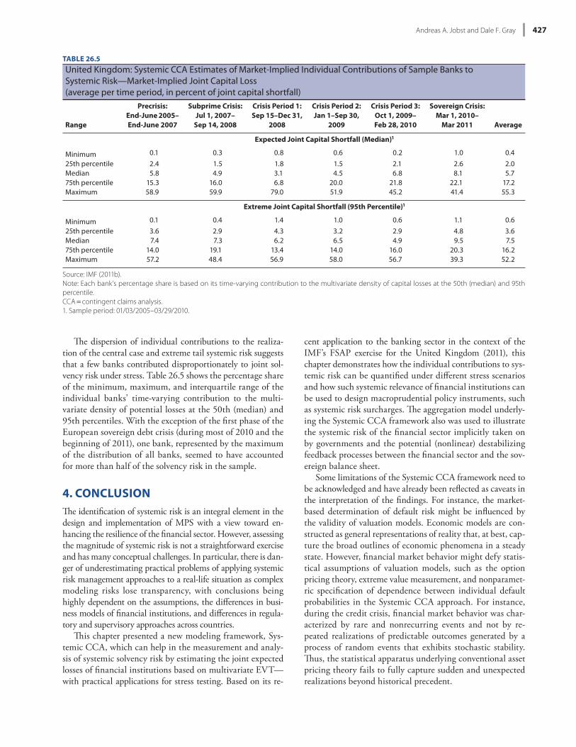
Andreas A. Jobst and Dale F. Gray 427
cent application to the banking sector in the context of the IMF’s FSAP exercise for the United Kingdom (2011), this chapter demonstrates how the individual contributions to sys-temic risk can be quantifi ed under diff erent stress scenarios and how such systemic relevance of fi nancial institutions can be used to design macroprudential policy instruments, such as systemic risk surcharges. Th e aggregation model underly-ing the Systemic CCA framework also was used to illustrate the systemic risk of the fi nancial sector implicitly taken on by governments and the potential (nonlinear) destabilizing feedback pro cesses between the fi nancial sector and the sov-ereign balance sheet.
Some limitations of the Systemic CCA framework need to be acknowledged and have already been refl ected as caveats in the interpretation of the fi ndings. For instance, the market- based determination of default risk might be infl uenced by the validity of valuation models. Economic models are con-structed as general repre sen ta tions of reality that, at best, cap-ture the broad outlines of economic phenomena in a steady state. However, fi nancial market behavior might defy statis-tical assumptions of valuation models, such as the option pricing theory, extreme value mea sure ment, and nonparamet-ric specifi cation of dependence between individual default probabilities in the Systemic CCA approach. For instance, during the credit crisis, fi nancial market behavior was char-acterized by rare and nonrecurring events and not by re-peated realizations of predictable outcomes generated by a pro cess of random events that exhibits stochastic stability. Th us, the statistical apparatus underlying conventional asset pricing theory fails to fully capture sudden and unexpected realizations beyond historical pre ce dent.
Th e dispersion of individual contributions to the realiza-tion of the central case and extreme tail systemic risk suggests that a few banks contributed disproportionately to joint sol-vency risk under stress. Table 26.5 shows the percentage share of the minimum, maximum, and interquartile range of the individual banks’ time- varying contribution to the multi-variate density of potential losses at the 50th (median) and 95th percentiles. With the exception of the fi rst phase of the Eu ro pe an sovereign debt crisis (during most of 2010 and the beginning of 2011), one bank, represented by the maximum of the distribution of all banks, seemed to have accounted for more than half of the solvency risk in the sample.
4. CONCLUSIONTh e identifi cation of systemic risk is an integral element in the design and implementation of MPS with a view toward en-hancing the resilience of the fi nancial sector. However, assessing the magnitude of systemic risk is not a straightforward exercise and has many conceptual challenges. In par tic u lar, there is dan-ger of underestimating practical problems of applying systemic risk management approaches to a real- life situation as complex modeling risks lose transparency, with conclusions being highly dependent on the assumptions, the diff erences in busi-ness models of fi nancial institutions, and diff erences in regula-tory and supervisory approaches across countries.
Th is chapter presented a new modeling framework, Sys-temic CCA, which can help in the mea sure ment and analy-sis of systemic solvency risk by estimating the joint expected losses of fi nancial institutions based on multivariate EVT— with practical applications for stress testing. Based on its re-
TABLE 26.5
United Kingdom: Systemic CCA Estimates of Market- Implied Individual Contributions of Sample Banks to Systemic Risk—Market- Implied Joint Capital Loss (average per time period, in percent of joint capital shortfall)
Range
Precrisis: End- June 2005–End- June 2007
Subprime Crisis: Jul 1, 2007–
Sep 14, 2008
Crisis Period 1: Sep 15– Dec 31,
2008
Crisis Period 2: Jan 1– Sep 30,
2009
Crisis Period 3: Oct 1, 2009– Feb 28, 2010
Sovereign Crisis: Mar 1, 2010–
Mar 2011 Average
Expected Joint Capital Shortfall (Median)
Minimum 0.1 0.3 0.8 0.6 0.2 1.0 0.4
25th percentile 2.4 1.5 1.8 1.5 2.1 2.6 2.0Median 5.8 4.9 3.1 4.5 6.8 8.1 5.775th percentile 15.3 16.0 6.8 20.0 21.8 22.1 17.2Maximum 58.9 59.9 79.0 51.9 45.2 41.4 55.3
Extreme Joint Capital Shortfall (95th Percentile)
Minimum 0.1 0.4 1.4 1.0 0.6 1.1 0.6
25th percentile 3.6 2.9 4.3 3.2 2.9 4.8 3.6Median 7.4 7.3 6.2 6.5 4.9 9.5 7.575th percentile 14.0 19.1 13.4 14.0 16.0 20.3 16.2Maximum 57.2 48.4 56.9 58.0 56.7 39.3 52.2
Source: IMF (2011b).Note: Each bank’s percentage share is based on its time- varying contribution to the multivariate density of capital losses at the 50th (median) and 95th percentile.CCA = contingent claims analysis.1. Sample period: 01/03/2005– 03/29/2010.
536-57355_IMF_StressTestHBk_ch03_3P.indd 427 11/5/14 2:06 AM
Systemic Contingent Claims Analysis 428
Basel Committee on Banking Supervision, 2012, “Results of the Basel III Monitoring Exercise as of 30 June 2011” (Basel, April 12). Available via the Internet: http:// www .bis .org /publ /bcbs217 .htm
Battiston, Stefano, Michelangelo Puliga, Rahul Kaushik, Paolo Tasca, and Guida Caldarelli, 2012, “DebtRank: Too Central to Fail? Financial Networks, the Fed and Systemic Risk,” Nature, August 2. Available via the Internet: http:// www .nature .com /srep /2012 /120802 /srep00541 /full /srep00541 .html
Black, Fischer, and John C. Cox, 1976, “Valuing Corporate Secu-rities: Some Eff ects on Bond Indenture Provisions,” Journal of Finance, Vol. 31, No. 2, pp. 351– 68.
Black, Fischer, and Myron Scholes, 1973, “Th e Pricing of Options and Corporate Liabilities,” Journal of Po liti cal Economy, Vol. 81, No. 3, pp. 637– 54.
Breeden, Douglas T., and Robert H. Litzenberger, 1978, “Prices of State- Contingent Claims Implicit in Option Prices,” Journal of Business, Vol. 51, No. 4, pp. 621– 51.
Brownlees, Christian T., and Robert F. Engle, 2011, “Volatility, Correlation and Tails for Systemic Risk Mea sure ment,” Work-ing Paper (New York: Stern School of Business, New York Uni-versity). Available via the Internet: http:// vleda .stern .nyu .edu /scrc /?p=2241
Carr, Peter, and Liuren Wu, 2007, “Th eory and Evidence on the Dynamic Interactions between Sovereign Credit Default Swaps and Currency Options,” Journal of Banking and Finance, Vol. 31, No. 8, pp. 2383– 403.
Chan- Lau, Jorge, 2010, “Regulatory Capital Charges for Too- Connected- to- Fail Institutions: A Practical Proposal,” IMF Working Paper 10/98 (Washington: International Monetary Fund). Available via the Internet: http:// www .imf .org /external /pubs /cat /longres .aspx ?sk=23753
Coles, Stuart G., Janet Heff ernan, and Jonathan A. Tawn, 1999, “Dependence Mea sures for Extreme Value Analyses,” Extremes, Vol. 2, pp. 339– 65.
Collin- Dufresne, Pierre, and Robert S. Goldstein, 2001, “Do Credit Spreads Refl ect Stationary Leverage Ratios?” Journal of Fi-nance, Vol. 56, No. 5, pp. 1929– 57.
Committee on the Global Financial System, 2012, “Operationalis-ing the Selection and Application of Macroprudential Instru-ments,” CGFS Papers No. 48, December (Basel: Committee on the Global Financial System). Available via the Internet: http:// www .bis .org /publ /cgfs48 .htm
Dall’Aglio, Georgio, Samuel I. Kotz, and Gabriella Salinetti, eds., 1991, Advances in Probability Distributions with Given Marginals (Beyond the Copulas) (Dordrecht: Kluwer Academic Publishers).
Drehmann, Mathias, and Nikola Tarashev, 2011, “Systemic Im-portance: Some Simple Indicators,” BIS Quarterly Review, pp. 25– 37 (Basel: Bank for International Settlements). Available via the Internet: http:// www .bis .org /publ /qtrpdf /r _qt1103 .htm
Duan, Jin- Chuan, 1994, “Maximum Likelihood Estimation Using Price Data of the Derivative Contract,” Mathematical Finance, Vol. 4, No. 2, pp. 155– 67.
Engle, Robert F., 2002, “Dynamic Conditional Correlation: A Simple Class of Multivariate Generalized Autoregressive Con-ditional Heteroskedasticity Models,” Journal of Business & Eco-nomic Statistics, Vol. 20, pp. 339– 50.
Engle, Robert F., and Kevin Sheppard, 2001, “Th eoretical and Empirical Properties of Dynamic Conditional Correlation Multivariate GARCH,” NBER Working Paper No. 8554 (Oc-tober). Available via the Internet: http:// www .nber .org /papers /w8554
Going forward, the Systemic CCA framework could be expanded in scale and scope to include other types of risks. For instance, most recently, the Systemic CCA framework also has been adapted to mea sure systemic liquidity risk by transforming the net stable funding ratio as standard liquidity mea sure under Basel III into a stochastic mea sure of aggregate funding risk (see Chapter 27). In addition, given the fl exibil-ity of this framework, the fi nancial sector and sovereign risk analysis could be integrated with macro- fi nancial feedbacks in order to design monetary and fi scal policies. Such an ap-proach could inform the calibration of stress scenarios of banking and sovereign balance sheets and the appropriate use of macroprudential regulation. Using an economy- wide Sys-temic CCA for all sectors, including the fi nancial sector, non-fi nancial corporates, house holds, and the government, also can provide new mea sures of economic output— the present value of risk- adjusted GDP (Gray, Jobst, and Malone, 2010).
REFERENCESAcharya, Viral V., Th omas F. Cooley, Matthew P. Richardson, and
Ingo Walter, eds., 2010, Regulating Wall Street: A New Architec-ture for Global Finance (Hoboken, NJ: Wiley).
Acharya, Viral V., Lasse H. Pedersen, Th omas Philippon, and Mat-thew P. Richardson, 2009, “Mea sur ing Systemic Risk,” Working Paper presented at the Federal Reserve Bank of Cleveland and the National Bureau of Economic Research “Research Conference on Quantifying Systemic Risk,” Cambridge, Massachusetts, No-vember 6. Available via the Internet: http:// www .clevelandfed .org /research /conferences /2009 /11 -6 -2009 /index .cfm
———, 2010, “Mea sur ing Systemic Risk,” FRBC Working Paper 10- 02 (Cleveland: Federal Reserve Bank of Cleveland). Avail-able via the Internet: http:// www .clevelandfed .org /research / workpaper /2010 /wp1002 .pdf
———, 2012, “Mea sur ing Systemic Risk,” CEPR Discussion Pa-per 8824, February. Available via the Internet: http:// www .cepr .org /pubs /dps /DP8824 .asp
Acharya, Viral V., Joao A. C. Santos, and Tanju Yorulmazer, 2010, “Systemic Risk and Deposit Insurance Premiums,” Economic Policy Review (New York: Federal Reserve Bank of New York, August).
Adrian, Tobias, and Markus K. Brunnermeier, 2008, “CoVaR,” Staff Report No. 348 (New York: Federal Reserve Bank of New York). Available via the Internet: http:// www .newyorkfed .org / research /staff _reports /sr348 .html
Aït- Sahalia, Yacine, and Andrew W. Lo, 1998, “Nonparametric Estimation of State- Price Densities Implicit in Financial Asset Prices, Journal of Finance, Vol. 53, No. 2, pp. 499– 547.
Allen, Franklin, Ana Babus, and Elena Carletti, 2010, “Financial Connections and Systemic Risk,” NBER Working Paper No. 16177 (Cambridge, MA: National Bureau of Economic Re-search). Available via the Internet: http:// www .nber .org /papers /w16177
Artzner, Philippe, Freddy Delbaen, Jean- Marc Eber, and David Heath, 1999, “Coherent Mea sures of Risk,” Mathematical Fi-nance, Vol. 9, No. 3, pp. 203– 28.
Backus, David, Silverio Foresi, and Liuren Wu, 2004, “Accounting for Biases in Black- Scholes,” Working Paper, New York Univer-sity, Goldman Sachs Group, and Baruch College.
536-57355_IMF_StressTestHBk_ch03_3P.indd 428 11/5/14 2:06 AM
Andreas A. Jobst and Dale F. Gray 429
Gray, Dale F., and Samuel Malone, 2010, “Quantifying Systemic Risk and Reconceptualizing the Role of Finance for Economic Growth,” Journal of Investment Management, Vol. 8, No. 2, pp. 90– 110.
Haldane, Andrew G., and Benjamin Nelson, 2012, “Tails of the Unexpected,” paper presented at “Th e Credit Crisis Five Years On: Unpacking the Crisis,” University of Edinburgh Business School conference, Edinburgh, June 8– 9. Available via the Inter-net: http:// www .bankofengland .co .uk /publications /Documents /speeches /2012 /speech582 .pdf
Hall, Peter, and Nader Tajvidi, 2000, “Distribution and Dependence- Function Estimation for Bivariate Extreme Value Distributions,” Bernoulli, Vol. 6, pp. 835– 44.
Huang, Xin, Hao Zhou, and Haibin Zhu, 2009, “A Framework for Assessing the Systemic Risk of Major Financial Institutions,” Journal of Banking and Finance, Vol. 33, No. 11, pp. 2036– 49.
———, 2010, “Assessing the Systemic Risk of a Heterogeneous Portfolio of Banks during the Recent Financial Crisis,” Working Paper No. 296 (Basel: Bank for International Settlements). Avail-able via the Internet: http:// www .bis .org /publ /work296 .htm
Hutchinson, Timothy P., and Chin D. Lai, 1990, Continuous Bivari-ate Distributions, Emphasizing Applications (Sydney: Rumsby Scientifi c Publishing).
International Monetary Fund, 2009a, “Assessing the Systemic Im-plications of Financial Linkages,” Global Financial Stability Re-port, Chapter 2 (Washington, April). Available via the Internet: http:// www .imf .org /External /Pubs /FT /GFSR /2009 /01 /index . htm
———, 2009b, “Detecting Systemic Risk,” Global Financial Stabil-ity Report, Chapter 3 (Washington, April). Available via the Inter-net: http:// www .imf .org /External /Pubs /FT /GFSR /2009 /01 /index .htm
———, 2010, “United States: Stress Testing— Technical Note,” IMF Country Report 10/244 (Washington, July 29). Available via the Internet: http:// www .imf .org /external /pubs /cat /longres .aspx ?sk=24101
———, 2011a, “Germany: Stress Testing— Technical Note,” IMF Country Report 11/371 (Washington, December 23). Available via the Internet: http:// www .imf .org /external /pubs /cat /longres .aspx ?sk=25461
———, 2011b, “Israel: Selected Issues,” IMF Country Report 11/23 (Washington, January 24). Available via the Internet: http:// www .imf .org /external /pubs /cat /longres .aspx ?sk=24587
———, 2011c, “Sweden: Contingent Claims Analysis Approach to Mea sure Risk and Stress Test the Swedish Banking Sector— Technical Note,” IMF Country Report 11/286 (Washington, September 1). Available via the Internet: http:// www .imf .org / external /pubs /cat /longres .aspx ?sk=25241
———, 2011d, “Toward Operationalizing Macroprudential Poli-cies: When to Act?,” Global Financial Stability Report, Chapter 3 (Washington, September). Available via the Internet: http:// www .imf .org /External /Pubs /FT /GFSR /2011 /02 /index .htm
———, 2011e, “United Kingdom: Stress Testing the Banking Sector— Technical Note,” IMF Country Report 11/227 (Wash-ington, July 1). Available via the Internet: http:// www .imf .org / external /pubs /cat /longres .aspx ?sk=25119
———, 2011f, “Th e United States: Spillover Report— 2011 Article IV Consultation,” IMF Country Report 11/203 (Washington, July 22). Available via the Internet: http:// www .imf .org /external /pubs /cat /longres .aspx ?sk=25083
———, 2012a, “Israel: Stress Test of the Banking, Insurance and Pension Sectors— Technical Note,” IMF Country Report 12/88
Ericsson, Jan, and Joel Reneby, 2004, “An Empirical Study of Structural Credit Risk Models Using Stock and Bond Prices,” Journal of Fixed Income, Vol. 13, No. 4, pp. 38– 49.
———, 2005, “Estimating Structural Bond Pricing Models,” Journal of Business, Vol. 78, No. 2, pp. 707– 35.
Espinosa- Vega, Marco, A., and Juan Solé, 2011, “Cross- Border Fi-nancial Surveillance: A Network Perspective,” Journal of Finan-cial Economic Policy, Vol. 3, No. 3, pp. 182– 205.
Financial Stability Board, International Monetary Fund, and Bank for International Settlements, 2011a, “Macroprudential Policy Tools and Frameworks,” Progress Report to the G-20 Finance Ministers and Central Bank Governors (Basel, October 26). Available via the Internet: http:// www .bis .org /publ /othp17 .pdf
———, 2011b, “Macroprudential Policy Tools and Frameworks,” Update to the G-20 Finance Ministers and Central Bank Gov-ernors (Basel, February 14). Available via the Internet: http:// www .bis .org /publ /othp13 .pdf
Fisher, Ronald A., and Leonard H. C. Tippett, 1928, “Limiting Forms of the Frequency Distribution of the Largest or Smallest Member of a Sample,” Proceedings of the Cambridge Philosophi-cal Society, Vol. 24, pp. 180– 90.
Gapen, Michael T., 2009, “Evaluating the Implicit Guarantee to Fannie Mae and Freddie Mac Using Contingent Claims,” International Finance Review: Credit, Capital, Currency, and Derivatives: Instruments of Global Financial Stability or Crisis?, Vol. 10, pp. 329– 52.
Gnedenko, Boris V., 1943, “Sur la Distribution Limite du Terme Maximum d’Une Série Aléatoire,” Annals of Mathematics, Vol. 44, pp. 423– 53.
González- Hermosillo, Brenda, Christian Capuano, Dale F. Gray, Heiko Hesse, Andreas A. Jobst, Paul Mills, Miguel Segoviano, and Tao Sun, 2009, “Methods to Identify Systemic Financial Risks,” Vox, April 23. Available via the Internet: http:// www . voxeu .org /index .php ?q=node /3495
Gray, Dale F., and Andreas A. Jobst, 2009a, “Higher Moments and Multivariate Dependence of Implied Volatilities from Equity Options as Mea sures of Systemic Risk,” Global Financial Stabil-ity Report, Chapter 3, pp. 128– 31 (Washington, April). Available via the Internet: http:// www .imf .org /External /Pubs /FT /GFSR /2009 /01 /index .htm
———, 2009b, “Using the CCA Framework to Estimate the Cost of Government Guarantees,” in “Crisis- Related Mea sures in the Financial System and Sovereign Balance Sheet Risks,” Board paper, edited by Adrienne Cheasty and Udaibir S. Das, Fiscal Aff airs and Monetary and Capital Markets Departments, July 31 (Washington: International Monetary Fund). Available via the Internet: http:// www .imf .org /external /np /sec /pn /2009 /pn09118 .htm
———, 2010, “New Directions in Financial Sector and Sovereign Risk Management, Journal of Investment Management, Vol. 8, No. 1, pp. 23– 38.
———, 2011a, “Modeling Systemic and Sovereign Risk,” in Les-sons from the Financial Crisis, edited by Arthur Berd, pp. 143– 85 (London: RISK Books).
———, 2011b, “Modelling Systemic Financial Sector and Sover-eign Risk,” Sveriges Riksbank Economic Review, No. 2, pp. 68– 106. Available via the Internet: http:// www .riksbank .se /upload /Rapporter /2011 /POV _2 /er _2011 _2 .pdf
———, 2011c, “Systemic Contingent Claims Analysis— A Model Approach to Systemic Risk,” in Managing Risk in the Financial System, edited by John R. LaBrosse, Rodrigo Olivares- Caminal, and Dalvinder Singh, pp. 93– 110 (London: Edward Elgar).
536-57355_IMF_StressTestHBk_ch03_3P.indd 429 11/5/14 2:06 AM
Systemic Contingent Claims Analysis 430
———, 1974, “On the Pricing of Corporate Debt: Th e Risk Structure of Interest Rates,” Journal of Finance, Vol. 29, No. 2, pp. 449– 70.
Ogden, Joseph P., 1987, “Determinants of the Ratings and Yields on Corporate Bonds: Tests of the Contingent Claims Model,” Jour-nal of Financial Research, Vol. 10, No. 4, pp. 329– 39.
Or ga ni za tion for Economic Cooperation and Development, 2012, “Systemic Financial Risk,” OECD Reviews of Risk Manage-ment Policies (Paris, June).
Pickands, James, 1981, “Multivariate Extreme Value Distributions,” Proceedings of the 43rd Session of the International Statistical Insti-tute, Vol. 49, pp. 859– 78.
Poon, Ser- Huan, Michael Rockinger, and Jonathan Tawn, 2003, “Extreme Value Dependence in Financial Markets: Diagnos-tics, Models, and Financial Implications,” Review of Financial Studies, Vol. 17, No. 2, pp. 581– 610.
Ronn, Ehud I., and Avinash K. Verma, 1986, “Pricing Risk- Adjusted Deposit Insurance: An Option- Based Model,” Journal of Finance, Vol. 41, No. 4, pp. 871– 95.
Rookley, Cameron, 1997, “Fully Exploiting the Information Con-tent of Intra Day Option Quotes: Applications in Option Pricing and Risk Management,” mimeo, University of Arizona.
Segoviano, Miguel A., and Charles A. E. Goodhart, 2009, “Banking Stability Measures,” IMF Working Paper 09/04 (Washington, International Monetary Fund).
Sedunov, John, III, 2012, “What Is the Systemic Risk Exposure of Financial Institutions?” mimeo, Villanova University, Depart-ment of Finance, September 1. Available via the Internet: http:// ssrn .com /abstract=2143633
Sklar, Abe, 1959, “Fonctions de Répartition à n Dimensions et Leurs Marges,” Publications de l’Institut de Statistique de L’Université de Paris, Vol. 8, pp. 229– 31.
Tarashev, Nicola, Claudio Borio, and Kostas Tsatsaronis, 2009, “Th e Systemic Importance of Financial Institutions,” BIS Quar-terly Review, pp. 75– 87 (Basel, September). Available via the In-ternet: http:// www .bis .org /publ /qtrpdf /r _qt0909 .htm
Weistroff er, Christian, 2011, “Identifying Systemically Important Financial Institutions (SIFIs),” International Topics— Current Issues, Deutsche Bank Research (August 11). Available via the Internet: http:// ideas .repec .org /p /ess /wpaper /id4383 .html
Wirch, Julia L., and Mary R. Hardy, 1999, “A Synthesis of Risk Mea sures for Capital Adequacy,” Insurance: Mathematics and Economics, Vol. 25, No. 3, pp. 337– 47.
Yu, Fan, 2006, “How Profi table Is Capital Structure Arbitrage?” Financial Analysts Journal, Vol. 62, No. 5, pp. 47– 62.
(Washington, April). Available via the Internet: http:// www .imf .org /external /pubs /cat /longres .aspx ?sk=25850
———, 2012b, “Spain: Financial System Stability Assessment,” IMF Country Report 12/137 (Washington, May 30). Available via the Internet: http:// www .imf .org /external /pubs /cat /longres .aspx ?sk=25977
———, Financial Stability Board, and Bank for International Set-tlements, 2009, “Guidance to Assess the Systemic Importance of Financial Institutions, Markets and Instruments: Initial Con-siderations,” Report to the G-20 Finance Ministers and Central Bank Governors, October. Available via the Internet: http:// www .imf .org /external /np /g20 /pdf /100109 .pdf
Jobst, Andreas A., 2007, “Operational Risk— Th e Sting Is Still in the Tail but the Poison Depends on the Dose,” Journal of Op-erational Risk, Vol. 2, No. 2, pp. 156.
———, 2013, “Multivariate Dependence of Implied Volatili-ties from Equity Options as Mea sure of Systemic Risk,” International Review of Financial Analysis, Vol. 28 ( June), pp. 112– 29.
———, 2014, “Mea sur ing Systemic Risk- Adjusted Liquidity (SRL)— A Model Approach,” Journal of Banking and Finance, Vol. 45, pp. 270–87.
———, and Dale F. Gray, 2013, “Systemic Contingent Claims Analysis— Estimating Market- Implied Systemic Risk,” IMF Working Paper 13/54 (Washington: International Monetary Fund). Available via the Internet: http:// www .imf .org /external /pubs /cat /longres .aspx ?sk=40356
———, and Herman Kamil, 2008, “Stock Market Linkages be-tween Latin America and the United States during ‘Tail Events,’ ” Regional Economic Outlook, Western Hemi sphere Department (Washington: International Monetary Fund).
Joe, Harry, 1997, Multivariate Models and Dependence Concepts, Monographs on Statistics and Applied Probability 73 (London: Chapman and Hall).
Jones, E. Philip, Scott P. Mason, and Eric Rosenfeld, 1984, “Con-tingent Claims Analysis of Corporate Capital Structures: An Empirical Investigation,” Journal of Finance, Vol. 39, No. 3, pp. 611– 25.
Longstaff , Francis A., and Eduardo S. Schwartz, 1995, “A Simple Approach to Valuing Risky Fixed and Floating Rate Debt,” Journal of Finance, Vol. 50, pp. 789– 819.
Merton, Robert C., 1973, “Th eory of Rational Option Pricing,” Bell Journal of Economics and Management Science, Vol. 4, No. 1, pp. 141– 83.
536-57355_IMF_StressTestHBk_ch03_3P.indd 430 11/5/14 2:06 AM


