Download - STATISTICA Logistic Regression - documentation.statsoft.com guide/Logistic... · STATISTICA Formula Guide Logistic Regression Version 1.1 4 Making the World More Productive® Column

STATISTICA Formula Guide Logistic Regression

Version 1.1 i

Making the World More Productive®

STATISTICA Formula Guide: Logistic Regression

Table of Contents Logistic Regression ...................................................................................................................................... 1

Overview of Logistic Regression Model .................................................................................................. 1

Dispersion ............................................................................................................................................... 2

Parameterization .................................................................................................................................... 3

Sigma-Restricted Model ...................................................................................................................... 3

Overparameterized Model ................................................................................................................. 4

Reference Coding ................................................................................................................................ 4

Model Summary (Summary Tab) ................................................................................................................ 5

Summary of All Effects ............................................................................................................................ 5

Wald Statistic ...................................................................................................................................... 5

Likelihood Ratio Test ........................................................................................................................... 6

Type 1 Likelihood Ratio Test ............................................................................................................... 7

Type 3 Likelihood Ratio Test ............................................................................................................... 7

Cell Statistics ........................................................................................................................................... 7

Mean ................................................................................................................................................... 8

Standard Deviation ............................................................................................................................. 8

Standard Error ..................................................................................................................................... 8

Upper/Lower Confidence Limits for the Mean ................................................................................... 9

Estimated Variance-Covariance Matrix .............................................................................................. 9

Estimated Correlation Matrix ............................................................................................................. 9

Parameter Estimates ........................................................................................................................... 9

Wald Statistic .................................................................................................................................... 10

Upper/Lower Confidence Limit for the Estimate ............................................................................. 10

Odds Ratio ......................................................................................................................................... 10

Confidence Limits for Odds Ratios .................................................................................................... 11

Classification of Cases and Odds Ratio ............................................................................................. 11

Iteration Results ................................................................................................................................ 12

Goodness of Fit ..................................................................................................................................... 12


Version 1.1 ii


Deviance ............................................................................................................................................ 12

Scaled Deviance ................................................................................................................................ 13

Pearson ......................................................................................................................................... 13

Scaled Pearson ............................................................................................................................. 13

Akaike Information Criterion (AIC) ................................................................................................... 14

Bayesian Information Criterion (BIC) ................................................................................................ 14

Cox-Snell R2 ....................................................................................................................................... 14

Nagelkerke R2 .................................................................................................................................... 15

Log-Likelihood ................................................................................................................................... 15

Testing Global Null Hypothesis ............................................................................................................. 15

Likelihood Ratio Test ......................................................................................................................... 15

Score Test .......................................................................................................................................... 15

Wald Test .......................................................................................................................................... 16

Hosmer-Lemeshow Test ................................................................................................................... 16

Aggregation ....................................................................................................................................... 17

Overdispersion .................................................................................................................................. 18

Residuals ................................................................................................................................................... 18

Basic Residuals ...................................................................................................................................... 18

Raw .................................................................................................................................................... 18

Pearson ............................................................................................................................................. 18

Deviance ............................................................................................................................................ 19

Predicted Values ................................................................................................................................... 19

Response ........................................................................................................................................... 19

Predicted Value ................................................................................................................................. 19

Linear Predictor ................................................................................................................................. 19

Standard Error of Linear Predictor .................................................................................................... 19

Upper/Lower Confidence Limits ....................................................................................................... 20

Leverage ............................................................................................................................................ 20

Studentized Pearson Residual .......................................................................................................... 20

Likelihood Residual ........................................................................................................................... 21

Other Obs. Stats .................................................................................................................................... 21


Version 1.1 iii


Gene al k’s D s ance ................................................................................................................... 21

Differential ................................................................................................................................... 22

Differential Deviance ........................................................................................................................ 22

Differential Likelihood ....................................................................................................................... 22

ROC Curve ......................................................................................................................................... 22

Lift Chart ............................................................................................................................................ 23

Observed, Unweighted Means ......................................................................................................... 24

Means of Groups ............................................................................................................................... 24

Observed, Weighted Means ............................................................................................................. 24

Means of Groups ............................................................................................................................... 24

Standard Error ................................................................................................................................... 25

Upper/Lower Confidence Limits of the Mean .................................................................................. 25

Predicted Means ............................................................................................................................... 25

Standard Error ................................................................................................................................... 26

Upper/Lower Confidence Limits of the Mean .................................................................................. 26

Model Building Summary .......................................................................................................................... 26

Stepwise Logistic Regression ................................................................................................................ 26

Forward Stepwise Method ................................................................................................................... 27

Backward Stepwise Method ................................................................................................................. 27

Forward Entry Method ......................................................................................................................... 27

Backward Entry Method ....................................................................................................................... 28

Wilson-Hilferty transformation ............................................................................................................ 28

Best Subsets .......................................................................................................................................... 28

References ................................................................................................................................................ 29


Version 1.1 1


Formula Guide

Logistic Regression

Logistic regression is used for modeling binary outcome variables such as credit default or warranty claims. It is assumed that the binary response, Y, takes on the values of 0 and 1 with 0 representing failure and 1 representing success.

Overview of Logistic Regression Model

The logistic regression function models the probability that the binary response is as a function of a set of predictor variables and regression coefficients as given by:

In practice, the regression coefficients are unknown and are estimated by maximizing the likelihood function. Note that the wi below are case weights and are assumed to be positive. All observations that have a case weight less than or equal to zero are excluded from the analysis and all subsequent results.

The maximization of the likelihood is achieved by an iterative method called Fisher scoring. Fisher scoring is similar to the Newton-Raphson procedure except that the hessian matrix (matrix of second order partial derivatives) is replaced with its expected value.

The Fisher scoring update formula for the regression coefficients is given by:

The algorithm completes when the convergence criterion is satisfied or when the maximum number of iterations has been reached. Convergence is obtained when the difference between the log-likelihood


Version 1.1 2


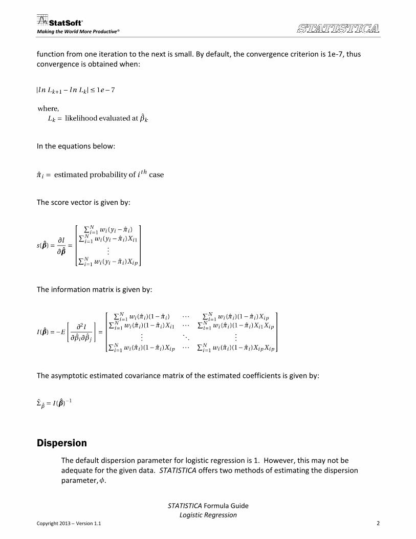
function from one iteration to the next is small. By default, the convergence criterion is 1e-7, thus convergence is obtained when:

In the equations below:

The score vector is given by:

The information matrix is given by:

The asymptotic estimated covariance matrix of the estimated coefficients is given by:

Dispersion

The default dispersion parameter for logistic regression is 1. However, this may not be adequate for the given data. STATISTICA offers two methods of estimating the dispersion parameter, . .


Version 1.1 3


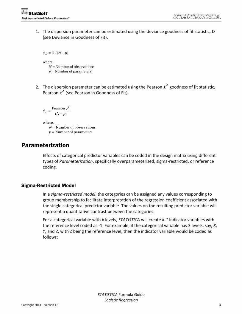
1. The dispersion parameter can be estimated using the deviance goodness of fit statistic, D (see Deviance in Goodness of Fit).

2. The dispersion parameter can be estimated using the Pearson goodness of fit statistic, Pearson (see Pearson in Goodness of Fit).

Parameterization

Effects of categorical predictor variables can be coded in the design matrix using different types of Parameterization, specifically overparameterized, sigma-restricted, or reference coding.

Sigma-Restricted Model

In a sigma-restricted model, the categories can be assigned any values corresponding to group membership to facilitate interpretation of the regression coefficient associated with the single categorical predictor variable. The values on the resulting predictor variable will represent a quantitative contrast between the categories.

For a categorical variable with k levels, STATISTICA will create k-1 indicator variables with the reference level coded as -1. For example, if the categorical variable has 3 levels, say, X, Y, and Z, with Z being the reference level, then the indicator variable would be coded as follows:


Version 1.1 4


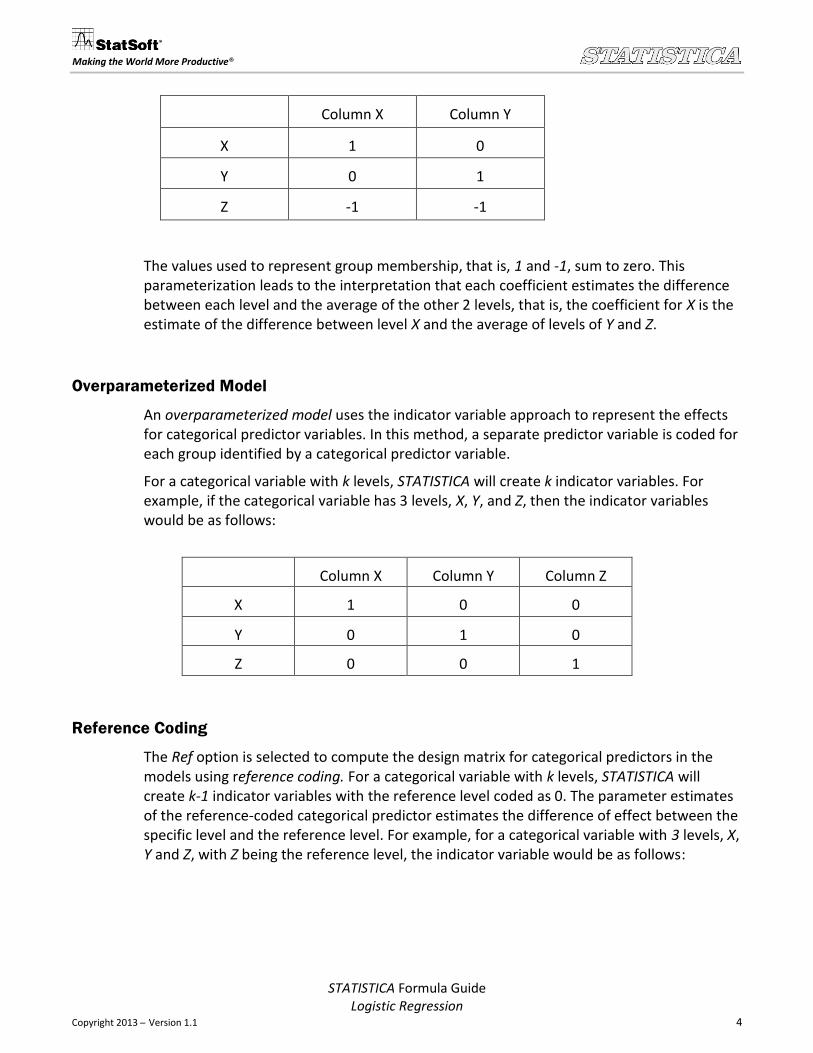
Column X Column Y

X 1 0

Y 0 1

Z -1 -1

The values used to represent group membership, that is, 1 and -1, sum to zero. This parameterization leads to the interpretation that each coefficient estimates the difference between each level and the average of the other 2 levels, that is, the coefficient for X is the estimate of the difference between level X and the average of levels of Y and Z.

Overparameterized Model

An overparameterized model uses the indicator variable approach to represent the effects for categorical predictor variables. In this method, a separate predictor variable is coded for each group identified by a categorical predictor variable.

For a categorical variable with k levels, STATISTICA will create k indicator variables. For example, if the categorical variable has 3 levels, X, Y, and Z, then the indicator variables would be as follows:

Column X Column Y Column Z

X 1 0 0

Y 0 1 0

Z 0 0 1

Reference Coding

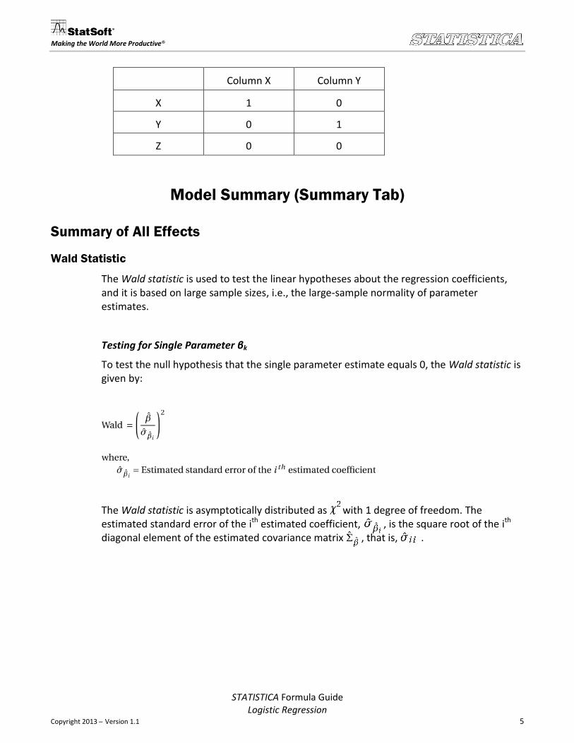
The Ref option is selected to compute the design matrix for categorical predictors in the models using reference coding. For a categorical variable with k levels, STATISTICA will create k-1 indicator variables with the reference level coded as 0. The parameter estimates of the reference-coded categorical predictor estimates the difference of effect between the specific level and the reference level. For example, for a categorical variable with 3 levels, X, Y and Z, with Z being the reference level, the indicator variable would be as follows:


Version 1.1 5


Column X Column Y

X 1 0

Y 0 1

Z 0 0

Model Summary (Summary Tab)

Summary of All Effects

Wald Statistic

The Wald statistic is used to test the linear hypotheses about the regression coefficients, and it is based on large sample sizes, i.e., the large-sample normality of parameter estimates.

Testing for Single Parameter βk

To test the null hypothesis that the single parameter estimate equals 0, the Wald statistic is given by:

The Wald statistic is asymptotically distributed as with 1 degree of freedom. The estimated standard error of the ith estimated coefficient, , is the square root of the ith diagonal element of the estimated covariance matrix , that is, .


Version 1.1 6


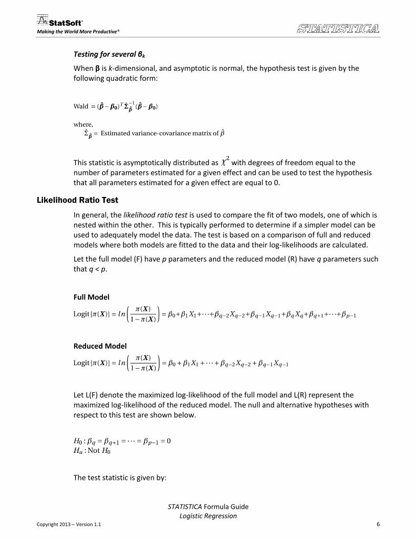
Testing for several βk

When β is k-dimensional, and asymptotic is normal, the hypothesis test is given by the following quadratic form:

This statistic is asymptotically distributed as with degrees of freedom equal to the number of parameters estimated for a given effect and can be used to test the hypothesis that all parameters estimated for a given effect are equal to 0.

Likelihood Ratio Test

In general, the likelihood ratio test is used to compare the fit of two models, one of which is nested within the other. This is typically performed to determine if a simpler model can be used to adequately model the data. The test is based on a comparison of full and reduced models where both models are fitted to the data and their log-likelihoods are calculated.

Let the full model (F) have p parameters and the reduced model (R) have q parameters such that q < p.

Full Model

Reduced Model

Let L(F) denote the maximized log-likelihood of the full model and L(R) represent the maximized log-likelihood of the reduced model. The null and alternative hypotheses with respect to this test are shown below.

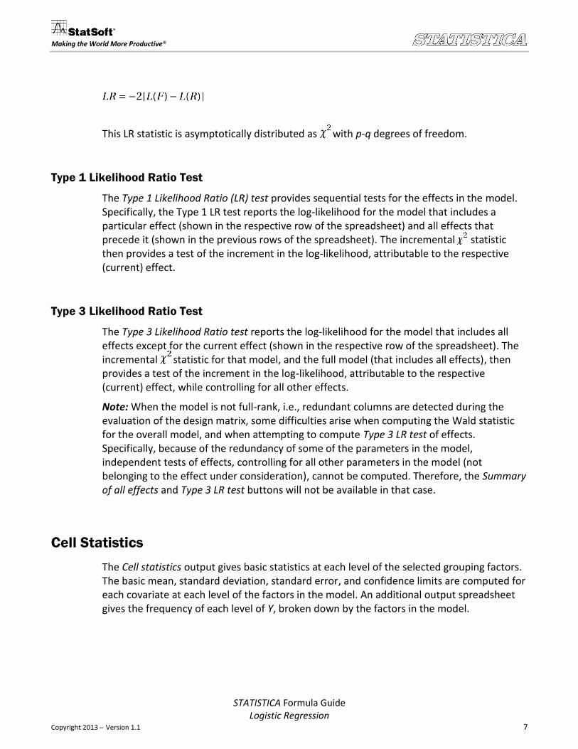
The test statistic is given by:


Version 1.1 7


This LR statistic is asymptotically distributed as with p-q degrees of freedom.

Type 1 Likelihood Ratio Test

The Type 1 Likelihood Ratio (LR) test provides sequential tests for the effects in the model. Specifically, the Type 1 LR test reports the log-likelihood for the model that includes a particular effect (shown in the respective row of the spreadsheet) and all effects that precede it (shown in the previous rows of the spreadsheet). The incremental statistic then provides a test of the increment in the log-likelihood, attributable to the respective (current) effect.

Type 3 Likelihood Ratio Test

The Type 3 Likelihood Ratio test reports the log-likelihood for the model that includes all effects except for the current effect (shown in the respective row of the spreadsheet). The incremental statistic for that model, and the full model (that includes all effects), then provides a test of the increment in the log-likelihood, attributable to the respective (current) effect, while controlling for all other effects.

Note: When the model is not full-rank, i.e., redundant columns are detected during the evaluation of the design matrix, some difficulties arise when computing the Wald statistic for the overall model, and when attempting to compute Type 3 LR test of effects. Specifically, because of the redundancy of some of the parameters in the model, independent tests of effects, controlling for all other parameters in the model (not belonging to the effect under consideration), cannot be computed. Therefore, the Summary of all effects and Type 3 LR test buttons will not be available in that case.

Cell Statistics

The Cell statistics output gives basic statistics at each level of the selected grouping factors. The basic mean, standard deviation, standard error, and confidence limits are computed for each covariate at each level of the factors in the model. An additional output spreadsheet gives the frequency of each level of Y, broken down by the factors in the model.

http://documentation.statsoft.com/STATISTICAHelp.aspx?path=Glossary/GlossaryTwo/D/DesignMatrix

http://documentation.statsoft.com/STATISTICAHelp.aspx?path=Glossary/GlossaryTwo/W/WaldStatistic


Version 1.1 8


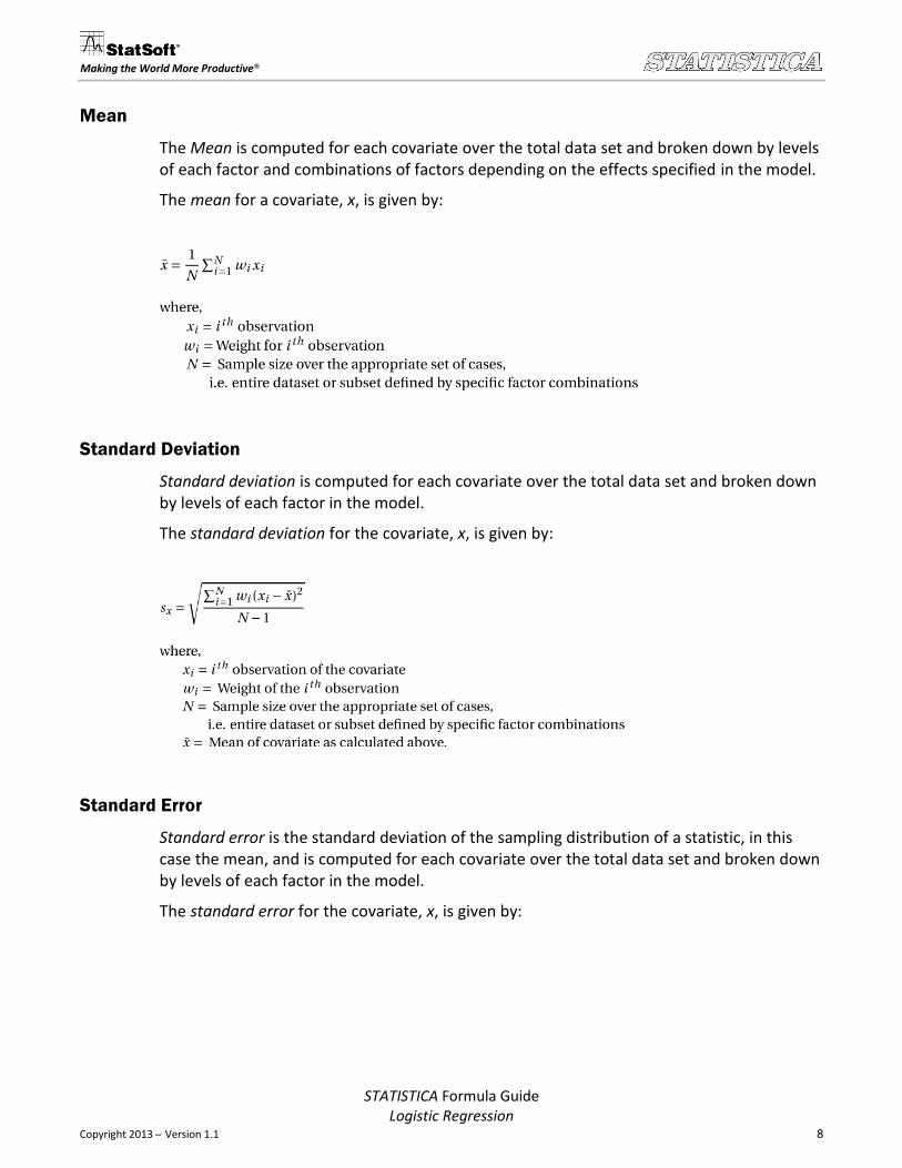
Mean

The Mean is computed for each covariate over the total data set and broken down by levels of each factor and combinations of factors depending on the effects specified in the model.

The mean for a covariate, x, is given by:

Standard Deviation

Standard deviation is computed for each covariate over the total data set and broken down by levels of each factor in the model.

The standard deviation for the covariate, x, is given by:

Standard Error

Standard error is the standard deviation of the sampling distribution of a statistic, in this case the mean, and is computed for each covariate over the total data set and broken down by levels of each factor in the model.

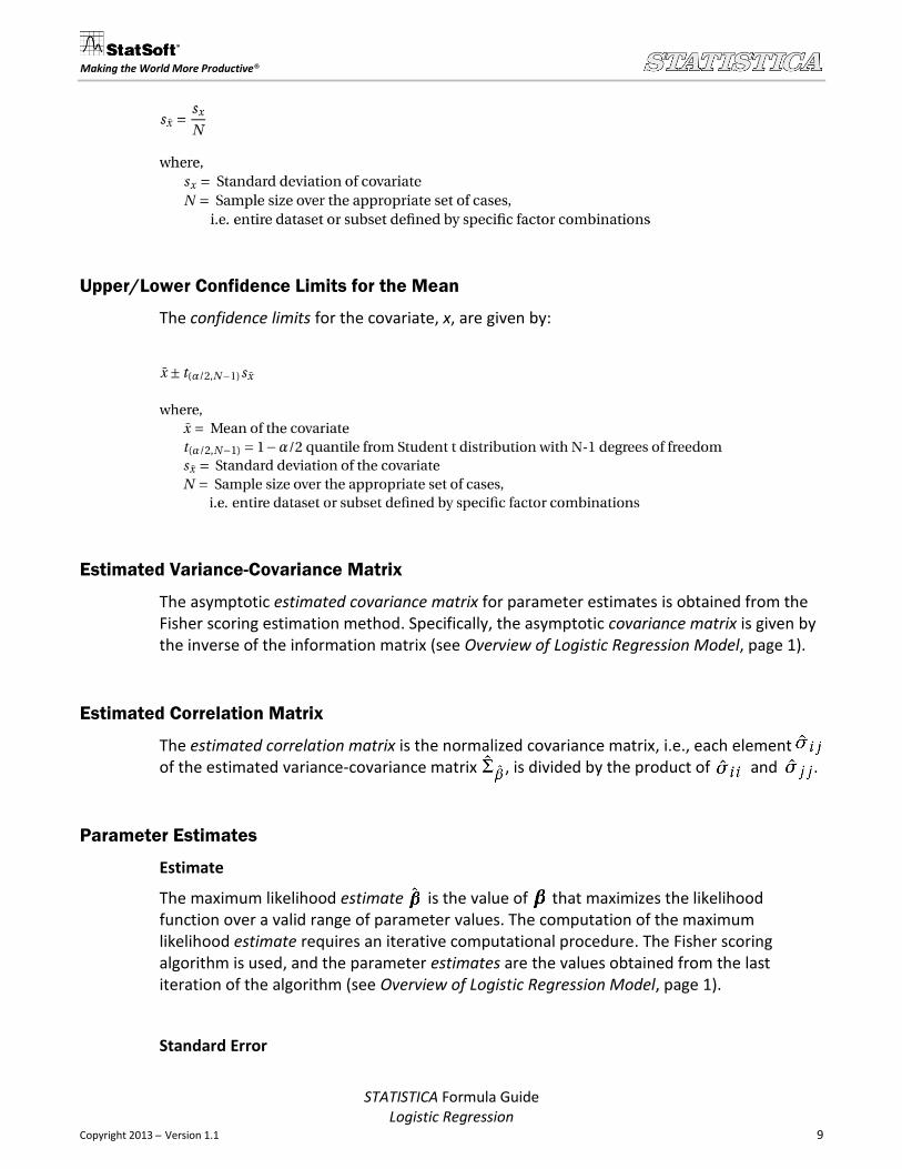
The standard error for the covariate, x, is given by:


Version 1.1 9


Upper/Lower Confidence Limits for the Mean

The confidence limits for the covariate, x, are given by:

Estimated Variance-Covariance Matrix

The asymptotic estimated covariance matrix for parameter estimates is obtained from the Fisher scoring estimation method. Specifically, the asymptotic covariance matrix is given by the inverse of the information matrix (see Overview of Logistic Regression Model, page 1).

Estimated Correlation Matrix

The estimated correlation matrix is the normalized covariance matrix, i.e., each element of the estimated variance-covariance matrix , is divided by the product of and .

Parameter Estimates

Estimate

The maximum likelihood estimate is the value of that maximizes the likelihood function over a valid range of parameter values. The computation of the maximum likelihood estimate requires an iterative computational procedure. The Fisher scoring algorithm is used, and the parameter estimates are the values obtained from the last iteration of the algorithm (see Overview of Logistic Regression Model, page 1).

Standard Error


Version 1.1 10


The standard error estimates are the square roots of the diagonals of the estimated variance-covariance matrix (see Estimated Variance-Covariance Matrix, page 9).

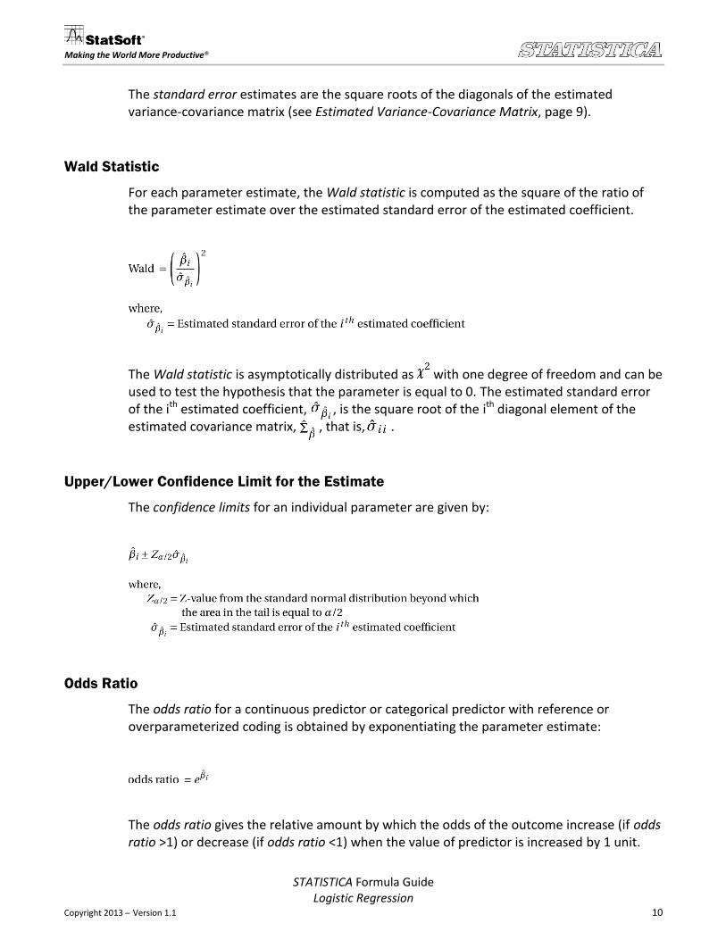
Wald Statistic

For each parameter estimate, the Wald statistic is computed as the square of the ratio of the parameter estimate over the estimated standard error of the estimated coefficient.

The Wald statistic is asymptotically distributed as with one degree of freedom and can be used to test the hypothesis that the parameter is equal to 0. The estimated standard error of the ith estimated coefficient, , is the square root of the ith diagonal element of the estimated covariance matrix, , that is, .

Upper/Lower Confidence Limit for the Estimate

The confidence limits for an individual parameter are given by:

Odds Ratio

The odds ratio for a continuous predictor or categorical predictor with reference or overparameterized coding is obtained by exponentiating the parameter estimate:

The odds ratio gives the relative amount by which the odds of the outcome increase (if odds ratio >1) or decrease (if odds ratio <1) when the value of predictor is increased by 1 unit.


Version 1.1 11


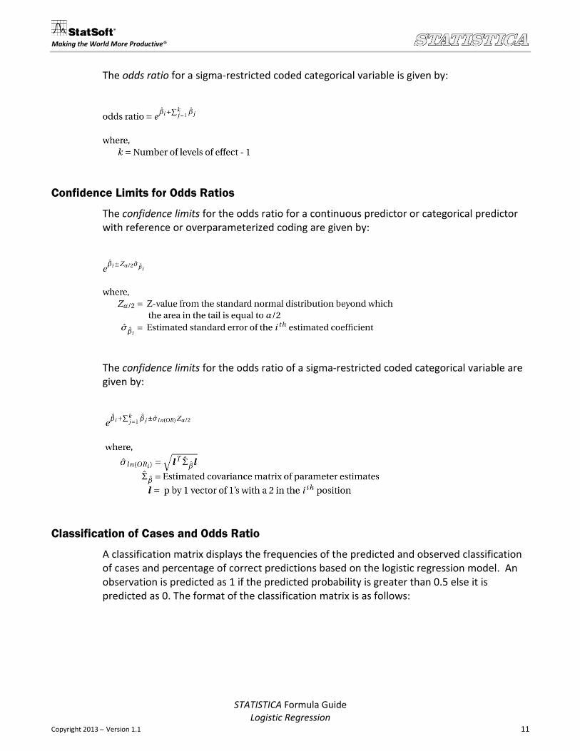
The odds ratio for a sigma-restricted coded categorical variable is given by:

Confidence Limits for Odds Ratios

The confidence limits for the odds ratio for a continuous predictor or categorical predictor with reference or overparameterized coding are given by:

The confidence limits for the odds ratio of a sigma-restricted coded categorical variable are given by:

Classification of Cases and Odds Ratio

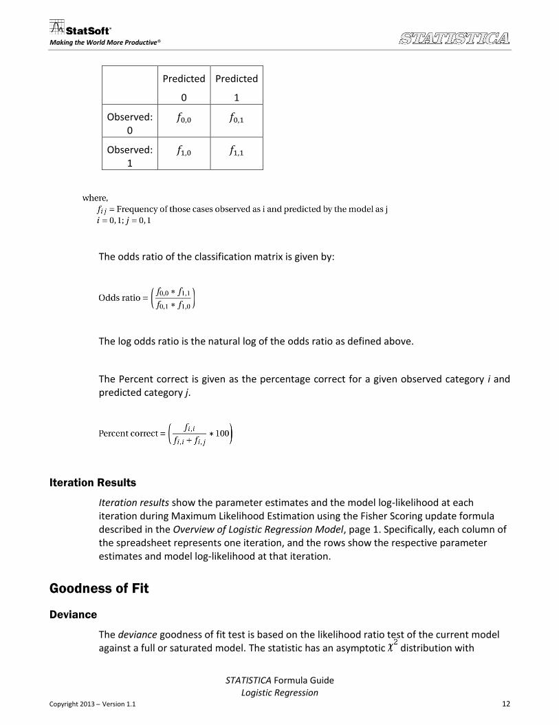
A classification matrix displays the frequencies of the predicted and observed classification of cases and percentage of correct predictions based on the logistic regression model. An observation is predicted as 1 if the predicted probability is greater than 0.5 else it is predicted as 0. The format of the classification matrix is as follows:


Version 1.1 12


Predicted

0

Predicted

1

Observed: 0

Observed: 1

The odds ratio of the classification matrix is given by:

The log odds ratio is the natural log of the odds ratio as defined above.

The Percent correct is given as the percentage correct for a given observed category i and predicted category j.

Iteration Results

Iteration results show the parameter estimates and the model log-likelihood at each iteration during Maximum Likelihood Estimation using the Fisher Scoring update formula described in the Overview of Logistic Regression Model, page 1. Specifically, each column of the spreadsheet represents one iteration, and the rows show the respective parameter estimates and model log-likelihood at that iteration.

Goodness of Fit

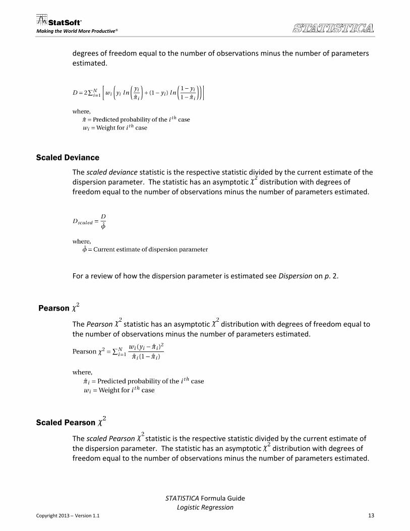
Deviance

The deviance goodness of fit test is based on the likelihood ratio test of the current model against a full or saturated model. The statistic has an asymptotic distribution with


Version 1.1 13


degrees of freedom equal to the number of observations minus the number of parameters estimated.

Scaled Deviance

The scaled deviance statistic is the respective statistic divided by the current estimate of the dispersion parameter. The statistic has an asymptotic distribution with degrees of freedom equal to the number of observations minus the number of parameters estimated.

For a review of how the dispersion parameter is estimated see Dispersion on p. 2.

Pearson

The Pearson statistic has an asymptotic distribution with degrees of freedom equal to the number of observations minus the number of parameters estimated.

Scaled Pearson

The scaled Pearson statistic is the respective statistic divided by the current estimate of the dispersion parameter. The statistic has an asymptotic distribution with degrees of freedom equal to the number of observations minus the number of parameters estimated.


Version 1.1 14


For a review of how the dispersion parameter is estimated see Dispersion on p. 2.

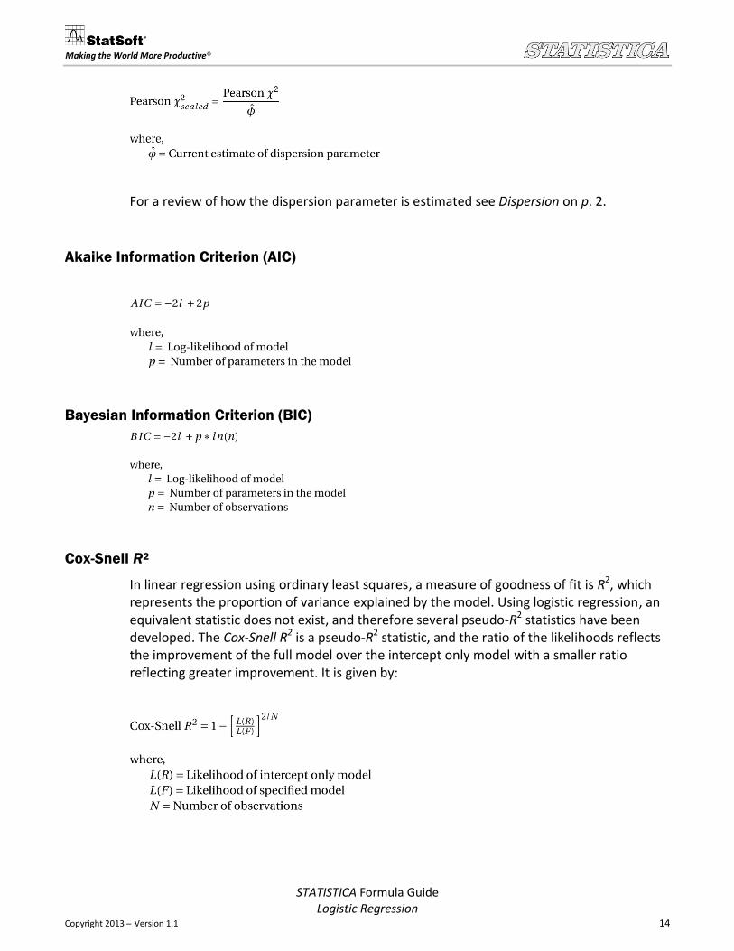
Akaike Information Criterion (AIC)

Bayesian Information Criterion (BIC)

Cox-Snell R2

In linear regression using ordinary least squares, a measure of goodness of fit is R2, which represents the proportion of variance explained by the model. Using logistic regression, an equivalent statistic does not exist, and therefore several pseudo-R2 statistics have been developed. The Cox-Snell R2 is a pseudo-R2 statistic, and the ratio of the likelihoods reflects the improvement of the full model over the intercept only model with a smaller ratio reflecting greater improvement. It is given by:


Version 1.1 15


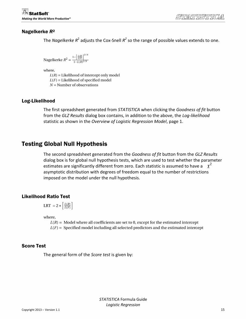
Nagelkerke R2

The Nagelkerke R2 adjusts the Cox-Snell R2 so the range of possible values extends to one.

Log-Likelihood

The first spreadsheet generated from STATISTICA when clicking the Goodness of fit button from the GLZ Results dialog box contains, in addition to the above, the Log-likelihood statistic as shown in the Overview of Logistic Regression Model, page 1.

Testing Global Null Hypothesis

The second spreadsheet generated from the Goodness of fit button from the GLZ Results dialog box is for global null hypothesis tests, which are used to test whether the parameter estimates are significantly different from zero. Each statistic is assumed to have a asymptotic distribution with degrees of freedom equal to the number of restrictions imposed on the model under the null hypothesis.

Likelihood Ratio Test

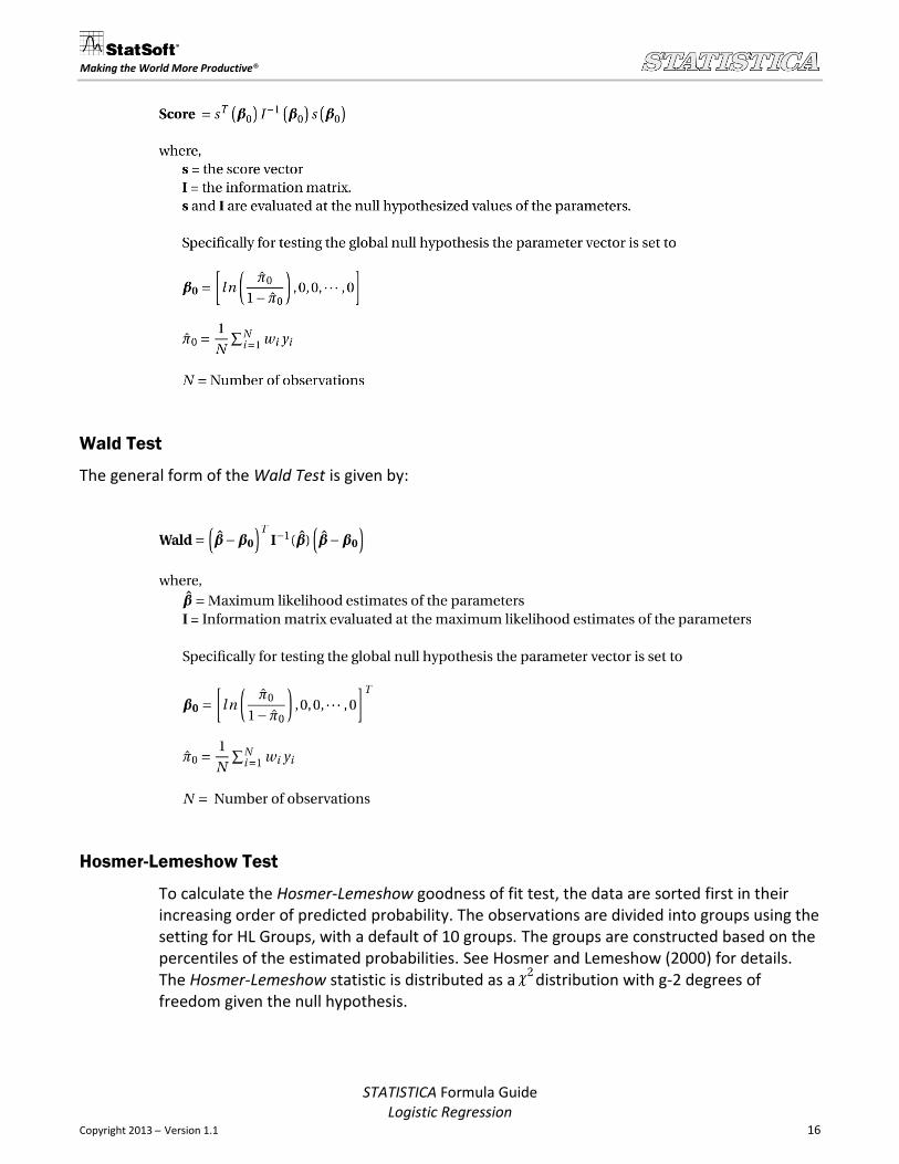
Score Test

The general form of the Score test is given by:


Version 1.1 16


Wald Test

The general form of the Wald Test is given by:

Hosmer-Lemeshow Test

To calculate the Hosmer-Lemeshow goodness of fit test, the data are sorted first in their increasing order of predicted probability. The observations are divided into groups using the setting for HL Groups, with a default of 10 groups. The groups are constructed based on the percentiles of the estimated probabilities. See Hosmer and Lemeshow (2000) for details. The Hosmer-Lemeshow statistic is distributed as a distribution with g-2 degrees of freedom given the null hypothesis.


Version 1.1 17


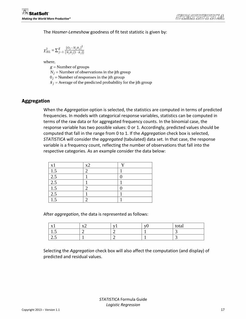
The Hosmer-Lemeshow goodness of fit test statistic is given by:

Aggregation

When the Aggregation option is selected, the statistics are computed in terms of predicted frequencies. In models with categorical response variables, statistics can be computed in terms of the raw data or for aggregated frequency counts. In the binomial case, the response variable has two possible values: 0 or 1. Accordingly, predicted values should be computed that fall in the range from 0 to 1. If the Aggregation check box is selected, STATISTICA will consider the aggregated (tabulated) data set. In that case, the response variable is a frequency count, reflecting the number of observations that fall into the respective categories. As an example consider the data below:

x1 x2 Y

1.5 2 1

2.5 1 0

2.5 1 1

1.5 2 0

2.5 1 1

1.5 2 1

After aggregation, the data is represented as follows:

x1 x2 y1 y0 total

1.5 2 2 1 3

2.5 1 2 1 3

Selecting the Aggregation check box will also affect the computation (and display) of predicted and residual values.


Version 1.1 18


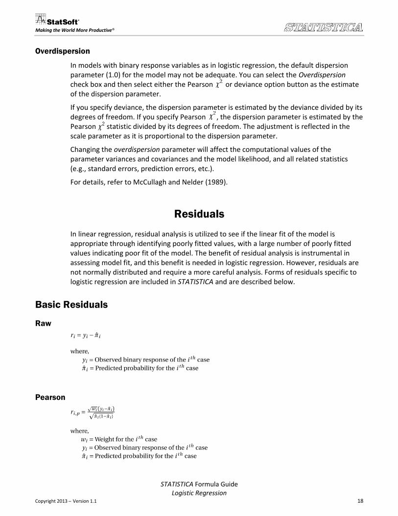
Overdispersion

In models with binary response variables as in logistic regression, the default dispersion parameter (1.0) for the model may not be adequate. You can select the Overdispersion check box and then select either the Pearson or deviance option button as the estimate of the dispersion parameter.

If you specify deviance, the dispersion parameter is estimated by the deviance divided by its degrees of freedom. If you specify Pearson , the dispersion parameter is estimated by the Pearson statistic divided by its degrees of freedom. The adjustment is reflected in the scale parameter as it is proportional to the dispersion parameter.

Changing the overdispersion parameter will affect the computational values of the parameter variances and covariances and the model likelihood, and all related statistics (e.g., standard errors, prediction errors, etc.).

For details, refer to McCullagh and Nelder (1989).

Residuals

In linear regression, residual analysis is utilized to see if the linear fit of the model is appropriate through identifying poorly fitted values, with a large number of poorly fitted values indicating poor fit of the model. The benefit of residual analysis is instrumental in assessing model fit, and this benefit is needed in logistic regression. However, residuals are not normally distributed and require a more careful analysis. Forms of residuals specific to logistic regression are included in STATISTICA and are described below.

Basic Residuals

Raw

Pearson


Version 1.1 19


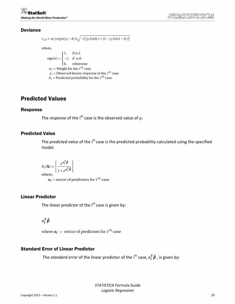
Deviance

Predicted Values

Response

The response of the ith case is the observed value of yi.

Predicted Value

The predicted value of the ith case is the predicted probability calculated using the specified model.

Linear Predictor

The linear predictor of the ith case is given by:

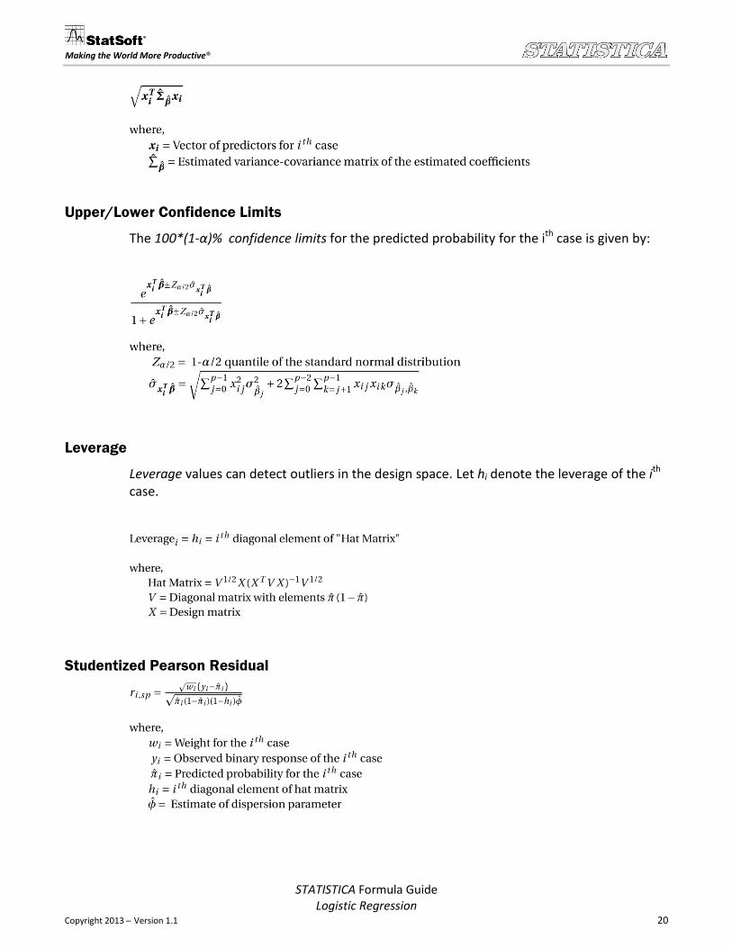
Standard Error of Linear Predictor

The standard error of the linear predictor of the ith case, , is given by:


Version 1.1 20


Upper/Lower Confidence Limits

The 100*(1-α)% confidence limits for the predicted probability for the ith case is given by:

Leverage

Leverage values can detect outliers in the design space. Let hi denote the leverage of the ith case.

Studentized Pearson Residual


Version 1.1 21


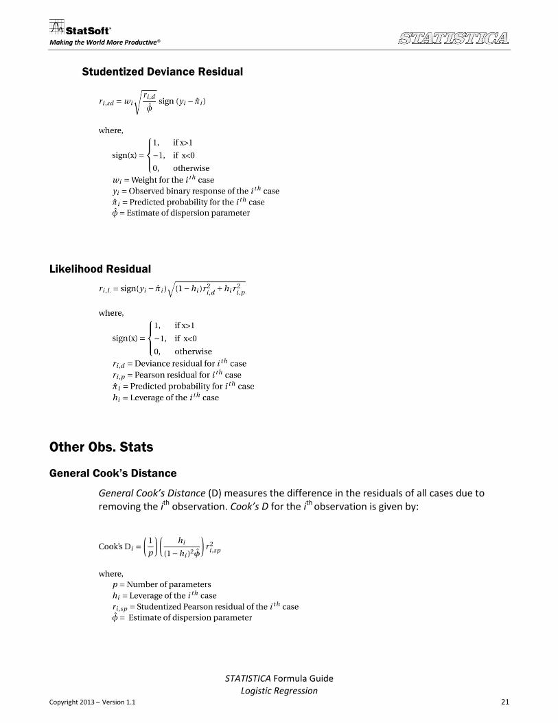
Studentized Deviance Residual

Likelihood Residual

Other Obs. Stats

General Cook’s Distance

General Cook’s Distance (D) measures the difference in the residuals of all cases due to removing the ith observation. Cook’s D for the ith observation is given by:


Version 1.1 22


Differential

The differential residual measures the difference in the Pearson statistic due to removing the ith observation.

Differential Deviance

The differential deviance residuals measure the difference in the deviance statistic due to removing the ith observation.

Differential Likelihood

The differential likelihood residuals measure the difference in the likelihood due to removing the ith observation.

ROC Curve

The ROC curve is often used as a measure of goodness-of-fit to evaluate the fit of a logistic regression model with a binary classifier. The plot is constructed using the true positive rate (rate of events that are correctly predicted as events and also called Sensitivity) on the y-axis against the false positive rate (rate of non-events predicted to be events also called 1-Specificity) on the x-axis for the different possible cutoff points based on the model


Version 1.1 23


The range of values for the predicted probabilities , Sensitivity and 1-Specificity, is provided in the corresponding spreadsheet. For each predicted probability, the algorithm iterates through each case to classify it as events or non-events using the predicted probability as the threshold value. The Sensitivity and 1-Specificity are calculated by:

The area under the ROC curve, sometimes also referred as Area Under Curve (AUC), gives a summary measure of the predictive power of the model, that is, the larger the AUC value (closer to 1), the better is the overall performance of the model to correctly classify the cases.

The AUC is computed using a nonparametric approach known as the trapezoidal rule. The area bounded by the curve and the baseline is divided into a series of trapezoidal regions (intervals) based on (1-Specifity, Sensitivity) points. The area is calculated for each region, and by summing the areas of the region, the total area under the ROC curve is computed.

Lift Chart

The lift chart provides a visual summary of the usefulness of the information provided by the logistic model for predicting a binomial dependent variable. The chart summarizes the utility (gain) that you can expect by using the respective predictive model shown by the Model curve as compared to using baseline information only.

Analogous lift values (Y-coordinate) that are calculated as the ratio between the results obtained with and without the predicted model can be computed for each percentile of the population sorted in descending order by the predicted value, that is, cases classified into the respective category with the highest classification probability. Each lift value indicates the effectiveness of a predictive model, that is, how many times it is better to use the model than not using one.

Let n be the number of true positives that appear in the top k% of the sorted list.


Version 1.1 24


Let r be the number of true positives that appear if we sort randomly, which is equal to the product of the total number of true positives and k.

Then,

The values for different percentiles can be connected by a line that will typically descend slowly and merge with the baseline.

Observed, Unweighted Means

Means of Groups

Observed, unweighted means are available for full factorial designs involving effects of 2 or more categorical factors. When cell frequencies in a multi-factor ANOVA design are equal, no difference exists between weighted and unweighted means. When cell frequencies are unequal, the unweighted means are calculated without adjusting for the differences between the sub-group frequencies. These are computed by averaging the means across the levels and combinations of levels of the factors not used in the marginal means table (or plot), and then dividing by the number of means in the average.

Observed, Weighted Means

Means of Groups

The mean of the dependent variable, y, for the jth level of the selected factor is given by:


Version 1.1 25


Standard Error

The standard error of the mean of the dependent variable, y for the jth level of the selected factor is given by:

Upper/Lower Confidence Limits of the Mean

Predicted Means

The predicted means are the expected value for the generalized linear model. When covariates are present in the model, predicted means are computed from the value of those covariates as set in the Covariate values group box. By default, covariates are set to their respective means.

The computation of the predicted means for each effect in the model is constructed by first generating the L matrix for the given effect. The L matrix is generated exactly in the same manner as in the General Linear Models (GLM) module when computing least square means which is also equivalent to how SAS® computes the L matrix. The vector of means on the logit scale for a given effect is then computed as .


Version 1.1 26


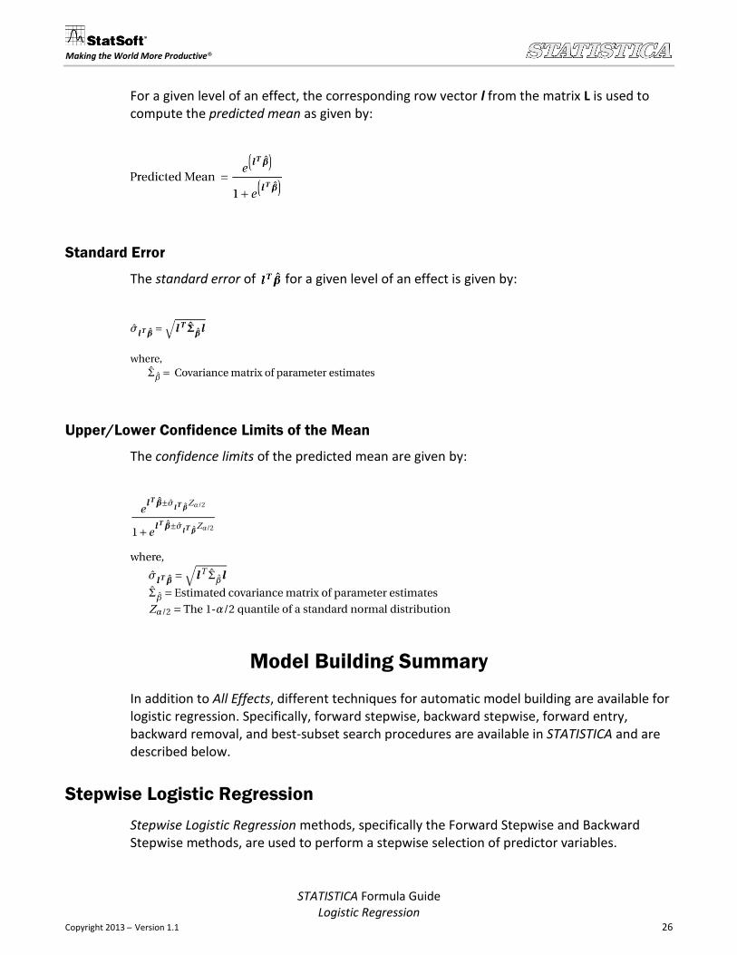
For a given level of an effect, the corresponding row vector l from the matrix L is used to compute the predicted mean as given by:

Standard Error

The standard error of for a given level of an effect is given by:

Upper/Lower Confidence Limits of the Mean

The confidence limits of the predicted mean are given by:

Model Building Summary

In addition to All Effects, different techniques for automatic model building are available for logistic regression. Specifically, forward stepwise, backward stepwise, forward entry, backward removal, and best-subset search procedures are available in STATISTICA and are described below.

Stepwise Logistic Regression

Stepwise Logistic Regression methods, specifically the Forward Stepwise and Backward Stepwise methods, are used to perform a stepwise selection of predictor variables.


Version 1.1 27


During the forward step of stepwise model building, if two or more effects have p-values that are so small as to be virtually indistinguishable from 0, STATISTICA will select the effect with the largest score statistic if the degrees of freedom for all effects in question are equal. If the effects differ with respect to the degrees of freedom, the Score statistics are normalized using the Wilson-Hilferty transformation, and the effect with the largest transformed value is entered into the model. For the backward step, if the p-values for two or more effects are virtually indistinguishable from 1, STATISTICA will remove the effect with the smallest Wald statistic in the case of equal degrees of freedom and the smallest normalized value in the case of unequal degrees of freedom.

Forward Stepwise Method

Let p be the number of total effects considered for the model. Let k be the number of effects currently in the model. Let p1, enter and p2, remove be specified by the user. The Forward Stepwise Method starts with no effects in the model and consists of two alternating steps, specifically

1. Entry step: For each of the remaining p-k effects not in the model, construct the p-k score statistics (see Testing Global Null Hypothesis, page 15, for a description of the score statistic). Enter the effect with the smallest p-value less than p1, enter.

2. Removal step: For all of the effects in the model compute the Wald statistic (see Testing Global Null Hypothesis, page 15, for a description of the score statistic). The effect with the largest p-value greater than p2, remove is removed from the model.

The procedure continues alternating between both steps until no further effects can either be added or removed or until the maximum number of steps (see the Max. steps option on the Advanced tab of the GLZ General Custom Design dialog box) has been reached.

Backward Stepwise Method

The Backward Stepwise Method is analogous to the Forward Stepwise Method; the only difference is that the initial model contains all the potential effects and begins attempting to remove effects and then subsequently attempts to enter them.

Forward Entry Method

The Forward Entry Method is the simplified version of Forward Stepwise Method. In this method, the step to test whether a variable already entered into the model should be removed is omitted. Specifically, the Forward Entry Method will only allow for effects to be entered into the model and does not allow for the removal of the variable once it has been added to the model.


Version 1.1 28


Backward Entry Method

The Backward Entry Method is the simplified version of the Backward Stepwise Method. It is the exact opposite of the Forward Entry Method.

As in the Backward Stepwise Method, this method begins with the model containing all potential predictors. It identifies the variable with the largest p-value, and if the p-value is greater than the p2, remove, the variable is dropped. This method eliminates the step of forward entering, or re-entering of the variable once it has been removed.

Wilson-Hilferty transformation

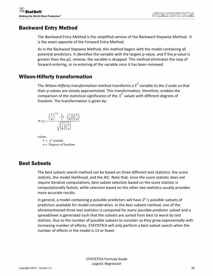
The Wilson-Hilferty transformation method transforms a variable to the Z-scale so that their p-values are closely approximated. This transformation, therefore, enables the comparison of the statistical significance of the values with different degrees of freedom. The transformation is given by:

Best Subsets

The best subsets search method can be based on three different test statistics: the score statistic, the model likelihood, and the AIC. Note that, since the score statistic does not require iterative computations, best subset selection based on the score statistic is computationally fastest, while selection based on the other two statistics usually provides more accurate results.

In general, a model containing p possible predictors will have 2p-1 possible subsets of predictors available for model consideration. In the best subsets method, one of the aforementioned three test statistics is computed for every possible predictor subset and a spreadsheet is generated such that the subsets are sorted from best to worst by test statistic. Due to the number of possible subsets to consider as they grow exponentially with increasing number of effects, STATISTICA will only perform a best subset search when the number of effects in the model is 13 or fewer.


Version 1.1 29


References

Agresti, A. (1990). Categorical Data Analysis. New York, NY: John Wiley & Sons, Inc.

Kutner, M., Nachtsheim, C., Neter, J. & Li, W. (2005). Applied linear statistical models (fifth

edition). New York, NY: McGraw-Hill Irwin

D.W. Hosmer and S. Lemeshow (2000). Applied Logistic Regression. 2nd ed. John Wiley & Sons,

Inc.

McCullagh, P. & Nelder, J. (1989). Generalized linear models (second edition). London, England:

Chapman & Hall

SAS Institute Inc. (2004). SAS 9.1.3 Help and Documentation, Cary, NC: SAS Institute Inc.

Download - STATISTICA Logistic Regression - documentation.statsoft.com guide/Logistic... · STATISTICA Formula Guide Logistic Regression Version 1.1 4 Making the World More Productive® Column

Top Related