Chapter 7
Random processes and noise
7.1 Introduction
Chapter 6 discussed modulation and demodulation, but replaced any detailed discussion of the noise by the assumption that a minimal separation is required between each pair of signal points. This chapter develops the underlying principles needed to understand noise, and the next chapter shows how to use these principles in detecting signals in the presence of noise.
Noise is usually the fundamental limitation for communication over physical channels. This can be seen intuitively by accepting for the moment that different possible transmitted waveforms must have a difference of some minimum energy to overcome the noise. This difference reflects back to a required distance between signal points, which along with a transmitted power constraint, limits the number of bits per signal that can be transmitted.
The transmission rate in bits per second is then limited by the product of the number of bits per signal times the number of signals per second, i.e., the number of degrees of freedom per second that signals can occupy. This intuitive view is substantially correct, but must be understood at a deeper level which will come from a probabilistic model of the noise.
This chapter and the next will adopt the assumption that the channel output waveform has the form y(t) = x(t) + z(t) where x(t) is the channel input and z(t) is the noise. The channel input x(t) depends on the random choice of binary source digits, and thus x(t) has to be viewed as a particular selection out of an ensemble of possible channel inputs. Similarly, z(t) is a particular selection out of an ensemble of possible noise waveforms.
The assumption that y(t) = x(t) + z(t) implies that the channel attenuation is known and removed by scaling the received signal and noise. It also implies that the input is not filtered or distorted by the channel. Finally it implies that the delay and carrier phase between input and output is known and removed at the receiver.
The noise should be modeled probabilistically. This is partly because the noise is a priori unknown, but can be expected to behave in statistically predictable ways. It is also because encoders and decoders are designed to operate successfully on a variety of different channels, all of which are subject to different noise waveforms. The noise is usually modeled as zero mean, since a mean can be trivially removed.
Modeling the waveforms x(t) and z(t) probabilistically will take considerable care. If x(t) and z(t) were defined only at discrete values of time, such as t = kT ; k ∈ Z, then they could
199
Cite as: Robert Gallager, course materials for 6.450 Principles of Digital Communications I, Fall 2006. MIT OpenCourseWare (http://ocw.mit.edu/), Massachusetts Institute of Technology. Downloaded on [DD Month YYYY].
200 CHAPTER 7. RANDOM PROCESSES AND NOISE
be modeled as sample values of sequences of random variables (rv’s). These sequences of rv’s could then be denoted as X(t) = X(kT ); k ∈ Z and Z(t) = Z(kT ); k ∈ Z. The case of interest here, however, is where x(t) and z(t) are defined over the continuum of values of t, and thus a continuum of rv’s is required. Such a probabilistic model is known as a random process or, synonomously, a stochastic process. These models behave somewhat similarly to random sequences, but they behave differently in a myriad of small but important ways.
7.2 Random processes
A random process Z(t); t ∈ R is a collection1 of rv’s, one for each t ∈ R. The parameter t usually models time, and any given instant in time is often referred to as an epoch. Thus there is one rv for each epoch. Sometimes the range of t is restricted to some finite interval, [a, b], and then the process is denoted as Z(t); t ∈ [a, b]. There must be an underlying sample space Ω over which these rv’s are defined. That is, for each epoch t ∈ R (or t ∈ [a, b]), the rv Z(t) is a function Z(t, ω); ω∈Ω mapping sample points ω ∈ Ω to real numbers.
A given sample point ω ∈ Ω within the underlying sample space determines the sample values of Z(t) for each epoch t. The collection of all these sample values for a given sample point ω, i.e., Z(t, ω); t ∈ R is called a sample function z(t) : R R of the process. →
Thus Z(t, ω) can be viewed as a function of ω for fixed t, in which case it is the rv Z(t), or it can be viewed as a function of t for fixed ω, in which case it is the sample function z(t) : R R = Z(t, ω); t ∈ R corresponding to the given ω. Viewed as a function of both t and ω,
→Z(t, ω); t ∈ R, ω ∈ Ω is the random process itself; the sample point ω is usually
suppressed, denoting the process as Z(t); t ∈ RSuppose a random process Z(t); t ∈ R models the channel noise and z(t) : R R is a sample →function of this process. At first this seems inconsistent with the traditional elementary view that a random process or set of rv’s models an experimental situation a priori (before performing the experiment) and the sample function models the result a posteriori (after performing the experiment). The trouble here is that the experiment might run from t = −∞ to t = ∞, so there can be no “before” for the experiment and “after” for the result.
There are two ways out of this perceived inconsistency. First, the notion of ‘before and after’ in the elementary view is inessential; the only important thing is the view that a multiplicity of sample functions might occur, but only one actually occurs. This point of view is appropriate in designing a cellular telephone for manufacture. Each individual phone that is sold experiences its own noise waveform, but the device must be manufactured to work over the multiplicity of such waveforms.
Second, whether we view a function of time as going from −∞ to +∞ or going from some large negative to large positive time is a matter of mathematical convenience. We often model waveforms as persisting from −∞ to +∞, but this simply indicates a situation in which the starting time and ending time are sufficiently distant to be irrelevant.
1Since a random variable is a mapping from Ω to R, the sample values of a rv are real and thus the sample functions of a random process are real. It is often important to define objects called complex random variables that map Ω to C. One can then define a complex random process as a process that maps each t ∈ R into a complex random variable. These complex random processes will be important in studying noise waveforms at baseband.
Cite as: Robert Gallager, course materials for 6.450 Principles of Digital Communications I, Fall 2006. MIT OpenCourseWare (http://ocw.mit.edu/), Massachusetts Institute of Technology. Downloaded on [DD Month YYYY].
7.2. RANDOM PROCESSES 201
In order to specify a random process Z(t); t ∈ R, some kind of rule is required from which joint distribution functions can, at least in principle, be calculated. That is, for all positive integers n, and all choices of n epochs t1, t2, . . . , tn, it must be possible (in principle) to find the joint distribution function,
FZ(t1),... ,Z(tn)(z1, . . . , zn) = PrZ(t1) ≤ z1, . . . , Z(tn) ≤ zn, (7.1)
for all choices of the real numbers z1, . . . , zn. Equivalently, if densities exist, it must be possible (in principle) to find the joint density,
∂nFZ(t1),... ,Z(tn)(z1, . . . , z )fZ(t1),... ,Z(tn)(z1, . . . , zn) =
∂zn
n, (7.2)
∂z1 · · ·for all real z1, . . . , zn. Since n can be arbitrarily large in (7.1) and (7.2), it might seem difficult for a simple rule to specify all these quantities, but a number of simple rules are given in the following examples that specify all these quantities.
7.2.1 Examples of random processes
The following generic example will turn out to be both useful and quite general. We saw earlier that we could specify waveforms by the sequence of coefficients in an orthonormal expansion. In the following example, a random process is similarly specified by a sequence of rv’s used as coefficients in an orthonormal expansion.
Example 7.2.1. Let Z1, Z2, . . . , be a sequence of rv’s defined on some sample space Ω and let φ1(t), φ2(t), . . . , be a sequence of orthogonal (or orthonormal) real functions. For each t ∈ R, let the rv Z(t) be defined as Z(t) = Zkφk(t). The corresponding random process k is then Z(t); t ∈ R. For each t, Z(t) is simply a sum of rv’s, so we could, in principle, find its distribution function. Similarly, for each n-tuple, t1, . . . , tn of epochs, Z(t1), . . . , Z(tn) is an n-tuple of rv’s whose joint distribution could in principle be found. Since Z(t) is a countably infinite sum of rv’s, ∞
k=1 Zkφk(t), there might be some mathematical intricacies in finding, or even defining, its distribution function. Fortunately, as will be seen, such intricacies do not arise in the processes of most interest here.
It is clear that random processes can be defined as in the above example, but it is less clear that this will provide a mechanism for constructing reasonable models of actual physical noise processes. For the case of Gaussian processes, which will be defined shortly, this class of models will be shown to be broad enough to provide a flexible set of noise models.
The next few examples specialize the above example in various ways.
Example 7.2.2. Consider binary PAM, but view the input signals as independent identically distributed (iid) rv’s U1, U2, . . . , which take on the values ±1 with probability 1/2 each. Assume that the modulation pulse is sinc( T
t ) so the baseband random process is
U(t) = Uk sinc t − kT
. T
k
At each sampling epoch kT , the rv U(kT ) is simply the binary rv Uk. At epochs between the sampling epochs, however, U(t) is a countably infinite sum of binary rv’s whose variance will later be shown to be 1, but whose distribution function is quite ugly and not of great interest.
Cite as: Robert Gallager, course materials for 6.450 Principles of Digital Communications I, Fall 2006. MIT OpenCourseWare (http://ocw.mit.edu/), Massachusetts Institute of Technology. Downloaded on [DD Month YYYY].
202 CHAPTER 7. RANDOM PROCESSES AND NOISE
Example 7.2.3. A random variable is said to be zero-mean Gaussian if it has the probability density
fZ (z) = √2
1
πσ2 exp[
−2σ
z2
2
], (7.3)
where σ2 is the variance of Z. A common model for a noise process Z(t); t ∈ R arises by letting
Z(t) = Zk sinc t − kT
, (7.4)T
k
where . . . , Z−1, Z0, Z1, . . . , is a sequence of iid zero-mean Gaussian rv’s of variance σ2. At each sampling epoch kT , the rv Z(kT ) is the zero-mean Gaussian rv Zk. At epochs between the sampling epochs, Z(t) is a countably infinite sum of independent zero-mean Gaussian rv’s, which turns out to be itself zero-mean Gaussian of variance σ2. The next section considers sums of Gaussian rv’s and their inter-relations in detail. The sample functions of this random process are simply sinc expansions and are limited to the baseband [−1/(2T ), 1/(2T )]. This example, as well as the previous example, brings out the following mathematical issue: the expected energy in Z(t); t ∈ R turns out to be infinite. As discussed later, this energy can be made finite either by truncating Z(t) to some finite interval much larger than any time of interest or by similarly truncating the sequence Zk; k ∈ Z. Another slightly disturbing aspect of this example is that this process cannot be ‘generated’ by a sequence of Gaussian rv’s entering a generating device that multiplies them by T -spaced sinc functions and adds them. The problem is the same as the problem with sinc functions in the previous chapter - they extend forever and thus the process cannot be generated with finite delay. This is not of concern here, since we are not trying to generate random processes, only to show that interesting processes can be defined. The approach here will be to define and analyze a wide variety of random processes, and then to see which are useful in modeling physical noise processes.
Example 7.2.4. Let Z(t); t ∈ [−1, 1] be defined by Z(t) = tZ for all t ∈ [−1, 1] where Z is a zero-mean Gaussian rv of variance 1. This example shows that random processes can be very degenerate; a sample function of this process is fully specified by the sample value z(t) at t = 1. The sample functions are simply straight lines through the origin with random slope. This illustrates that the sample functions of a random process do not necessarily “look” random.
7.2.2 The mean and covariance of a random process
Often the first thing of interest about a random process is the mean at each epoch t and the covariance between any two epochs t, τ . The mean, E[Z(t)] = Z(t) is simply a real valued function of t and can be found directly from the distribution function FZ(t)(z) or density fZ(t)(z). It can be verified that Z(t) is 0 for all t for Examples 7.2.2, 7.2.3, and 7.2.4 above. For Example 7.2.1, the mean can not be specified without specifying more about the random sequence and the orthogonal functions.
The covariance2 is a real-valued function of the epochs t and τ . It is denoted by KZ (t, τ) and 2This is often called the autocovariance to distinguish it from the covariance between two processes; we will
not need to refer to this latter type of covariance.
Cite as: Robert Gallager, course materials for 6.450 Principles of Digital Communications I, Fall 2006. MIT OpenCourseWare (http://ocw.mit.edu/), Massachusetts Institute of Technology. Downloaded on [DD Month YYYY].
7.2. RANDOM PROCESSES 203
defined by
KZ (t, τ) = E [Z(t) − Z(t)][Z(τ) − Z(τ)] . (7.5)
This can be calculated (in principle) from the joint distribution function FZ(t),Z(τ)(z1, z2) or from the density fZ(t),Z(τ )(z1, z2). To make the covariance function look a little simpler, we usually split each random variable Z(t) into its mean, Z(t), and its fluctuation, Z(t) = Z(t)− Z(t). The covariance function is then
KZ (t, τ) = E Z(t)Z(τ) . (7.6)
The random processes of most interest to us are used to model noise waveforms and usually have zero mean, in which case Z(t) = Z(t). In other cases, it often aids intuition to separate the process into its mean (which is simply an ordinary function) and its fluctuation, which is by definition zero mean.
The covariance function for the generic random process in Example 7.2.1 above can be written as
KZ (t, τ) = E Zkφk(t) Zmφm(τ) . (7.7) k m
If we assume that the rv’s Z1, Z2, . . . are iid with variance σ2, then E[ZkZm] = 0 for k = m and E[ZkZm] = σ2 for k = m. Thus, ignoring convergence questions, (7.7) simplifies to
KZ (t, τ) = σ2 φk(t)φk(τ). (7.8) k
For the sampling expansion, where φk(t) = sinc( t − k), it can be shown (see (7.48)) that the T sum in (7.8) is simply sinc( t−
Tτ ). Thus for Examples 7.2.2 and 7.2.3, the covariance is given by
KZ (t, τ) = σ2sinc t − τ
T
where σ2 = 1 for the binary PAM case of Example 7.2.2. Note that this covariance depends only on t − τ and not on the relationship between t or τ and the sampling points kT . These sampling processes are considered in more detail later.
7.2.3 Additive noise channels
The communication channels of greatest interest to us are known as additive noise channels. Both the channel input and the noise are modeled as random processes, X(t); t ∈ R and Z(t); t ∈ R, both on the same underlying sample space Ω. The channel output is another random process Y (t); t ∈ R and Y (t) = X(t) + Z(t). This means that for each epoch t the random variable Y (t) is equal to X(t) + Z(t).
Note that one could always define the noise on a channel as the difference Y (t) − X(t) between output and input. The notion of additive noise inherently also includes the assumption that the processes X(t); t ∈ R and Z(t); t ∈ R are statistically independent.3
3More specifically, this means that for all k > 0, all epochs t1, . . . , tk, and all epochs τ1, . . . , τk, the rvs X(t1), . . . , X(tk) are statistically independent of Z(τ1), . . . , Z(τk).
Cite as: Robert Gallager, course materials for 6.450 Principles of Digital Communications I, Fall 2006. MIT OpenCourseWare (http://ocw.mit.edu/), Massachusetts Institute of Technology. Downloaded on [DD Month YYYY].

204 CHAPTER 7. RANDOM PROCESSES AND NOISE
As discussed earlier, the additive noise model Y (t) = X(t) + Z(t) implicitly assumes that the channel attenuation, propagation delay, and carrier frequency and phase are perfectly known and compensated for. It also assumes that the input waveform is not changed by any disturbances other than the noise, Z(t).
Additive noise is most frequently modeled as a Gaussian process, as discussed in the next section. Even when the noise is not modeled as Gaussian, it is often modeled as some modification of a Gaussian process. Many rules of thumb in engineering and statistics about noise are stated without any mention of Gaussian processes, but are often valid only for Gaussian processes.
7.3 Gaussian random variables, vectors, and processes
This section first defines Gaussian random variables (rv’s), then jointly-Gaussian random vectors (rv’s), and finally Gaussian random processes. The covariance function and joint density function for Gaussian random vectors are then derived. Finally several equivalent conditions for rv’s to be jointly Gaussian are derived.
A rv W is a normalized Gaussian rv, or more briefly a normal4 rv, if it has the probability density
fW (w) = √12π
exp −
2 w2
.
This density is symmetric around 0 and thus the mean of W is zero. The variance is 1, which is probably familiar from elementary probability and is demonstrated in Exercise 7.1. A random variable Z is a Gaussian rv if it is a scaled and shifted version of a normal rv, i.e., if Z = σW +Z ¯ for a normal rv W . It can be seen that Z ¯ is the mean of Z and σ2 is the variance5. The density of Z (for σ2 > 0) is
fZ (z) = √2
1
πσ2 exp
−((2z− σ2
Z
))2
. (7.9)
A Gaussian rv Z of mean Z ¯ and variance σ2 is denoted as Z ∼ N ( ¯ Z, σ2). The Gaussian rv’s used to represent noise are almost invariably zero-mean. Such rv’s have the density fZ(z) = √
2
1
πσ2 exp[−z2
] and are denoted by Z ∼ N (0, σ2).2σ2
Zero-mean Gaussian rv’s are important in modeling noise and other random phenomena for the following reasons:
• They serve as good approximations to the sum of many independent zero-mean rv’s (recall the central limit theorem).
• They have a number of extremal properties; as discussed later, they are, in several senses, the most random rv’s for a given variance.
• They are easy to manipulate analytically, given a few simple properties.
• They serve as common channel noise models, and in fact the literature often assumes that noise is modeled by zero-mean Gaussian rv’s without explicitly stating it.
4Some people use normal rv as a synonym for Gaussian rv. 5It is convenient to denote Z as Gaussian even in the deterministic case where σ = 0, but (7.9) is invalid then.
Cite as: Robert Gallager, course materials for 6.450 Principles of Digital Communications I, Fall 2006. MIT OpenCourseWare (http://ocw.mit.edu/), Massachusetts Institute of Technology. Downloaded on [DD Month YYYY].
7.3. GAUSSIAN RANDOM VARIABLES, VECTORS, AND PROCESSES 205
Definition 7.3.1. A set of n of random variables, Z1, . . . , Zn is zero-mean jointly Gaussian if there is a set of iid normal rv’s W1, . . . , W such that each Zk, 1 ≤ k ≤ n, can be expressed as
Zk = akmWm; 1 ≤ k ≤ n, (7.10) m=1
where akm; 1≤k≤n, 1≤m≤ is an array of real numbers. Z1′ , . . . , Zn
′ is jointly Gaussian if Zk
′ = Zk + Z k′ where the set Z1, . . . , Zn is zero-mean jointly Gaussian and Z
1′ , . . . , Z
n′ is a set of
real numbers.
It is convenient notationally to refer to a set of n random variables, Z1, . . . , Zn as a random vector6 (rv) Z = (Z1, . . . , Zn)T . Letting A be the n by real matrix with elements akm; 1≤k≤n, 1≤m≤ , (7.10) can then be represented more compactly as
Z = A W . (7.11)
Similarly the jointly-Gaussian random vector Z ′ above can be represented as Z ′ = AZ + Z ′
where Z ′ is an n-vector of real numbers.
In the remainder of this chapter, all random variables, random vectors, and random processes are assumed to be zero-mean unless explicitly designated otherwise. Viewed differently, only the fluctuations are analyzed with the means added at the end7 .
It is shown in Exercise 7.2 that any sum m akmWm of iid normal rv’s W1, . . . , Wn is a Gaussian rv, so that each Zk in (7.10) is Gaussian. Jointly Gaussian means much more than this, however. The random variables Z1, . . . , Zn must also be related as linear combinations of the same set of iid normal variables. Exercises 7.3 and 7.4 illustrate some examples of pairs of random variables which are individually Gaussian but not jointly Gaussian. These examples are slightly artificial, but illustrate clearly that the joint density of jointly-Gaussian rv’s is much more constrained than the possible joint densities arising from constraining marginal distributions to be Gaussian.
The above definition of jointly Gaussian looks a little contrived at first, but is in fact very natural. Gaussian rv’s often make excellent models for physical noise processes because noise is often the summation of many small effects. The central limit theorem is a mathematically precise way of saying that the sum of a very large number of independent small zero-mean random variables is approximately zero-mean Gaussian. Even when different sums are statistically dependent on each other, they are different linear combinations of a common set of independent small random variables. Thus the jointly-Gaussian assumption is closely linked to the assumption that the noise is the sum of a large number of small, essentially independent, random disturbances. Assuming that the underlying variables are Gaussian simply makes the model analytically clean and tractable.
An important property of any jointly-Gaussian n-dimensional rv Z is the following: for any real m by n real matrix B, the rv Y = BZ is also jointly Gaussian. To see this, let Z = AW where W is a normal rv. Then
Y = BZ = B(AW ) = (BA)W . (7.12)
6The class of random vectors for a given n over a given sample space satisfies the axioms of a vector space, but here the vector notation is used simpy as a notational convenience.
7When studying estimation and conditional probabilities, means become an integral part of many arguments, but these arguments will not be central here.
Cite as: Robert Gallager, course materials for 6.450 Principles of Digital Communications I, Fall 2006. MIT OpenCourseWare (http://ocw.mit.edu/), Massachusetts Institute of Technology. Downloaded on [DD Month YYYY].
206 CHAPTER 7. RANDOM PROCESSES AND NOISE
Since BA is a real matrix, Y is jointly Gaussian. A useful application of this property arises when A is diagonal, so Z has arbitrary independent Gaussian components. This implies that Y = BZ is jointly Gaussian whenever a rv Z has independent Gaussian components.
Another important application is where B is a 1 by n matrix and Y is a random variable. Thus every linear combination k
n =1 bkZk of a jointly-Gaussian rv Z = (Z1, . . . , Zn)T is Gaussian. It
will be shown later in this section that this is an if and only if property; that is, if every linear combination of a rv Z is Gaussian, then Z is jointly Gaussian.
We now have the machinery to define zero-mean Gaussian processes.
Definition 7.3.2. Z(t); t ∈ R is a zero-mean Gaussian process if, for all positive integers n and all finite sets of epochs t1, . . . , tn, the set of random variables Z(t1), . . . , Z(tn) is a (zeromean) jointly-Gaussian set of random variables.
If the covariance, KZ (t, τ) = E[Z(t)Z(τ)], is known for each pair of epochs t, τ , then for any finite set of epochs t1, . . . , tn, E [Z(tk)Z(tm)] is known for each pair (tk, tm) in that set. The next two subsections will show that the joint probability density for any such set of (zero-mean) jointly-Gaussian rv’s depends only on the covariances of those variables. This will show that a zero-mean Gaussian process is specified by its covariance function. A nonzero-mean Gaussian process is similarly specified by its covariance function and its mean.
7.3.1 The covariance matrix of a jointly-Gaussian random vector
Let an n-tuple of (zero-mean) random variables (rv’s) Z1, . . . , Zn be represented as a random vector (rv) Z = (Z1, . . . , Zn)T . As defined in the previous section, Z is jointly Gaussian if Z = AW where W = (W1, W2, . . . , W)T is a vector of iid normal rv’s and A is an n by real matrix. Each rv Zk, and all linear combinations of Z1, . . . , Zn, are Gaussian.
The covariance of two (zero-mean) rv’s Z1, Z2 is E[Z1Z2]. For a rv Z = (Z1, . . . Zn)T the covariance between all pairs of random variables is very conveniently represented by the n by n covariance matrix,
KZ = E[ZZ T].
Appendix 7A.1 develops a number of properties of covariance matrices (including the fact that they are identical to the class of nonnegative definite matrices). For a vector W = W1, . . . , W
of independent normalized Gaussian rv’s, E[Wj Wm] = 0 for j = m and 1 for j = m. Thus
KW = E[WW T] = I,
where I is the by identity matrix. For a zero-mean jointly-Gaussian vector Z = AW , the covariance matrix is thus
KZ = E[AWW TAT] = AE[WW T]AT = AAT . (7.13)
The probability density, fZ (z ), of a rv Z = (Z1, Z2, . . . , Zn)T is the joint probability density of the components Z1, . . . , Zn. An important example is the iid rv W where the components Wk, 1 ≤ k ≤ n, are iid and normal, Wk ∼ N (0, 1). By taking the product of the n densities of the individual random variables, the density of W = (W1, W2, . . . , Wn)T is
fW (w) =1
exp −w1
2 − w22 − · · · − wn
2
= 1
exp −‖w‖2
. (7.14)(2π)n/2 2 (2π)n/2 2
Cite as: Robert Gallager, course materials for 6.450 Principles of Digital Communications I, Fall 2006. MIT OpenCourseWare (http://ocw.mit.edu/), Massachusetts Institute of Technology. Downloaded on [DD Month YYYY].

7.3. GAUSSIAN RANDOM VARIABLES, VECTORS, AND PROCESSES 207
This shows that the density of W at a sample value w depends only on the squared distance ‖w‖2 of the sample value from the origin. That is, fW (w) is spherically symmetric around the origin, and points of equal probability density lie on concentric spheres around the origin.
7.3.2 The probability density of a jointly-Gaussian random vector
Consider the transformation Z = AW where Z and W each have n components and A is n by n. If we let a1,a2, . . . ,an be the n columns of A, then this means that Z = m W. That is,am m
for any sample values w1, . . . wn for W , the corresponding sample value for Z is z = m amwm. Similarly, if we let b1, . . . , bn be the rows of A, then Zk = bkW .
Let Bδ be a cube, δ on a side, of the sample values of W defined by Bδ = w : 0≤wk≤δ; 1≤k≤n(see Figure 7.1). The set Bδ
′ of vectors z = Aw for w ∈ Bδ is a parallepiped whose sides are the vectors δa1, . . . , δan. The determinant, det(A), of A has the remarkable geometric property that its magnitude, | det(A)|, is equal to the volume of the parallelepiped with sides ak; 1 ≤ k ≤ n. Thus the unit cube Bδ above, with volume δn, is mapped by A into a parallelepiped of volume | det A|δn .
0δ
δ
w1
w2
z1
z2
δa1 δa2
Figure 7.1: Example illustrating how Z = AW maps cubes into parallelepipeds. Let Z1 = −W1 + 2W2 and Z2 = W1 + W2. The figure shows the set of sample pairs z1, z2
corresponding to 0 ≤ w1 ≤ δ and 0 ≤ w2 ≤ δ. It also shows a translation of the same cube mapping into a translation of the same parallelepiped.
Assume that the columns a1, . . . ,an are linearly independent. This means that the columns must form a basis for Rn, and thus that every vector z is some linear combination of these columns, i.e., that z = Aw for some vector w . The matrix A must then be invertible, i.e., there is a matrix A−1 such that AA−1 = A−1A = In where In is the n by n identity matrix. The matrix A maps the unit vectors of Rn into the vectors a1, . . . ,an and the matrix A−1 maps a1, . . . ,an
back into the unit vectors.
If the columns of A are not linearly independent, i.e., A is not invertible, then A maps the unit cube in Rn into a subspace of dimension less than n. In terms of Fig. 7.1, the unit cube would be mapped into a straight line segment. The area, in 2 dimensional space, of a straight line segment is 0, and more generally, the volume in n-space of a lower dimensional set of points is 0. In terms of the determinant, det A = 0 for any noninvertible matrix A.
Assuming again that A is invertible, let z be a sample value of Z , and let w = A−1 z be the corresponding sample value of W . Consider the incremental cube w + Bδ cornered at w . For δ very small, the probability Pδ(w) that W lies in this cube is fW (w)δn plus terms that go to zero faster than δn as δ → 0. This cube around w maps into a parallelepiped of volume δn| det(A)|around z , and no other sample value of W maps into this parallelepiped. Thus Pδ(w) is also
Cite as: Robert Gallager, course materials for 6.450 Principles of Digital Communications I, Fall 2006. MIT OpenCourseWare (http://ocw.mit.edu/), Massachusetts Institute of Technology. Downloaded on [DD Month YYYY].
| |
208 CHAPTER 7. RANDOM PROCESSES AND NOISE
equal to fZ (z )δn| det(A)| plus negligible terms. Going to the limit δ → 0, we have
Pδ(w)fZ (z ) det(A) = lim = fW (w). (7.15)| |
δ→0 δn
Since w = A−1 z , we get the explicit formula
fW (A−1 z )fZ (z ) = . (7.16) | det(A)|
This formula is valid for any random vector W with a density, but we are interested in the vector W of iid Gaussian random variables, N (0, 1). Substituting (7.14) into (7.16),
fZ (z ) = (2π)n/2
1det(A)
exp −‖A−
2
1z‖2
(7.17)
1 1 =
(2π)n/2| det(A)| exp −2z T(A−1)TA−1 z (7.18)
We can simplify this somewhat by recalling from (7.13) that the covariance matrix of Z is givenby KZ = AAT. Thus K−
Z 1 = (A−1)TA−1 .
Substituting this into (7.18) and noting that det(KZ ) = | det(A)|2 ,
1 1 TK−1fZ (z ) = (2π)n/2
det(KZ )
exp −2z Z z . (7.19)
Note that this probability density depends only on the covariance matrix of Z and not directly on the matrix A.
The above density relies on A being nonsingular. If A is singular, then at least one of its rows is a linear combination of the other rows, and thus, for some m, 1 ≤ m ≤ n, Zm is a linear combination of the other Zk. The random vector Z is still jointly Gaussian, but the joint probability density does not exist (unless one wishes to view the density of Zm as a unit impulse at a point specified by the sample values of the other variables). It is possible to write out the distribution function for this case, using step functions for the dependent rv’s, but it is not worth the notational mess. It is more straightforward to face the problem and find the density of a maximal set of linearly independent rv’s, and specify the others as deterministic linear combinations.
It is important to understand that there is a large difference between rv’s being statistically dependent and linearly dependent. If they are linearly dependent, then one or more are deterministic functions of the others, whereas statistical dependence simply implies a probabilistic relationship.
These results are summarized in the following theorem:
Theorem 7.3.1 (Density for jointly-Gaussian rv’s). Let Z be a (zero-mean) jointly-Gaussian rv with a nonsingular covariance matrix KZ. Then the probability density fZ(z) is given by (7.19). If KZ is singular, then fZ(z) does not exist but the density in (7.19) can be applied to any set of linearly independent rv’s out of Z1, . . . , Zn.
For a zero-mean Gaussian process Z(t), the covariance function KZ (t, τ) specifies E [Z(tk)Z(tm)] for arbitrary epochs tk and tm and thus specifies the covariance matrix for any finite set of epochs
Cite as: Robert Gallager, course materials for 6.450 Principles of Digital Communications I, Fall 2006. MIT OpenCourseWare (http://ocw.mit.edu/), Massachusetts Institute of Technology. Downloaded on [DD Month YYYY].
7.3. GAUSSIAN RANDOM VARIABLES, VECTORS, AND PROCESSES 209
t1, . . . , tn. From the above theorem, this also specifies the joint probability distribution for that set of epochs. Thus the covariance function specifies all joint probability distributions for all finite sets of epochs, and thus specifies the process in the sense8 of Section 7.2. In summary, we have the following important theorem.
Theorem 7.3.2 (Gaussian process). A zero-mean Gaussian process is specified by its covariance function K(t, τ ).
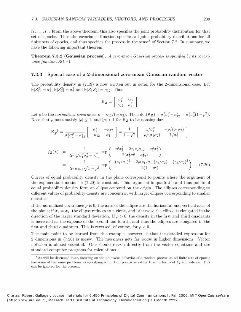
7.3.3 Special case of a 2-dimensional zero-mean Gaussian random vector
The probability density in (7.19) is now written out in detail for the 2-dimensional case. Let E[Z1
2] = σ12 , E[Z2
2] = σ22 and E[Z1Z2] = κ12. Thus
σ2 κ12KZ = 1 . κ12 σ2
2
Let ρ be the normalized covariance ρ = κ12/(σ1σ2). Then det(KZ ) = σ12σ2
2 −κ21σ2
2(1−ρ2).12 = σ2
Note that ρ must satisfy |ρ| ≤ 1, and |ρ| < 1 for KZ to be nonsingular.
K−1 =1 σ2
2 −κ12 =1 1/σ1
2 −ρ/(σ1σ2) .Z σ12σ2
2 − κ2 −κ12 σ12 1 − ρ2 −ρ/(σ1σ2) 1/σ2
12 2
fZ (z ) = 1 exp
−z12σ2 + 2z1z2κ12 − z2
2σ2 2 1
2π σ2σ22 − κ2 2(σ2σ2
2 − κ2 )1 12 1 12
1 −(z1/σ1)2 + 2ρ(z1/σ1)(z2/σ2) − (z2/σ2)2 = exp . (7.20)2πσ1σ2 1 − ρ2 2(1 − ρ2)
Curves of equal probability density in the plane correspond to points where the argument of the exponential function in (7.20) is constant. This argument is quadratic and thus points of equal probability density form an ellipse centered on the origin. The ellipses corresponding to different values of probability density are concentric, with larger ellipses corresponding to smaller densities.
If the normalized covariance ρ is 0, the axes of the ellipse are the horizontal and vertical axes of the plane; if σ1 = σ2, the ellipse reduces to a circle, and otherwise the ellipse is elongated in the direction of the larger standard deviation. If ρ > 0, the density in the first and third quadrants is increased at the expense of the second and fourth, and thus the ellipses are elongated in the first and third quadrants. This is reversed, of course, for ρ < 0.
The main point to be learned from this example, however, is that the detailed expression for 2 dimensions in (7.20) is messy. The messiness gets far worse in higher dimensions. Vector notation is almost essential. One should reason directly from the vector equations and use standard computer programs for calculations.
8As will be discussed later, focusing on the pointwise behavior of a random process at all finite sets of epochs has some of the same problems as specifying a function pointwise rather than in terms of L2 equivalence. This can be ignored for the present.
Cite as: Robert Gallager, course materials for 6.450 Principles of Digital Communications I, Fall 2006. MIT OpenCourseWare (http://ocw.mit.edu/), Massachusetts Institute of Technology. Downloaded on [DD Month YYYY].
210 CHAPTER 7. RANDOM PROCESSES AND NOISE
7.3.4 Z = AW where A is orthogonal
An n by n real matrix A for which AAT = In is called an orthogonal matrix or orthonormal matrix (orthonormal is more appropriate, but orthogonal is more common). For Z = AW , where W is iid normal and A is orthogonal, KZ = AAT = In. Thus K−
Z 1 = In also and (7.19)
becomes
T 2 2 kfZ (z ) =
exp(2−π)
1
n/
z2
z =
n exp[√−2z
π
/2] . (7.21)
k=1
This means that A transforms W into a random vector Z with the same probability density, and thus the components of Z are still normal and iid. To understand this better, note that AAT = In means that AT is the inverse of A and thus that ATA = In. Letting am be the mth
column of A, the equation ATA = In means that aT a j = δmj for each m, j, 1≤m, j≤n, i.e., that m
the columns of A are orthonormal. Thus, for the two dimensional example, the unit vectors e1, e2 are mapped into orthonormal vectors a1,a2, so that the transformation simply rotates the points in the plane. Although it is difficult to visualize such a transformation in higher dimensional space, it is still called a rotation, and has the property that ||Aw ||2 = wTATAw , which is just wTw = ||w ||2 . Thus, each point w maps into a point Aw at the same distance from the origin as itself.
Not only the columns of an orthogonal matrix are orthonormal, but the rows, say bk; 1≤k≤nare also orthonormal (as is seen directly from AAT = In). Since Zk = bkW , this means that, for any set of orthonormal vectors b1, . . . , bn, the random variables Zk = bkW are normal and iid for 1 ≤ k ≤ n.
7.3.5 Probability density for Gaussian vectors in terms of principal axes
This subsection describes what is often a more convenient representation for the probability density of an n-dimensional (zero-mean) Gaussian rv Z with a nonsingular covariance matrix KZ . As shown in Appendix 7A.1, the matrix KZ has n real orthonormal eigenvectors, q1, . . . , qn, with corresponding nonnegative (but not necessarily distinct9) real eigenvalues, λ1, . . . , λn. Also, for any vector z , it is shown that z TK−
Z 1 z can be expressed as k λ
−k
1|〈z , qk〉|2 . Substituting this in (7.19), we have
fZ (z ) = (2π)n/2
1det(KZ )
exp − |〈z
2,
λ
q
k
k〉|2 . (7.22)
k
Note that 〈z , qk〉 is the projection of z on the kth of n orthonormal directions. The determinant of an n by nreal matrix can be expressed in terms of the n eigenvalues (see Appendix 7A.1) as det(KZ ) = k
n =1 λk. Thus (7.22) becomes
n fZ (z ) =
√
21 πλk
exp −|〈z
2,
λ
q
k
k〉|2 . (7.23)
k=1
9If an eigenvalue λ has multiplicity m, it means that there is an m dimensional subspace of vectors q satisfying KZq = λq ; in this case any orthonormal set of m such vectors can be chosen as the m eigenvectors corresponding to that eigenvalue.
Cite as: Robert Gallager, course materials for 6.450 Principles of Digital Communications I, Fall 2006. MIT OpenCourseWare (http://ocw.mit.edu/), Massachusetts Institute of Technology. Downloaded on [DD Month YYYY].
7.3. GAUSSIAN RANDOM VARIABLES, VECTORS, AND PROCESSES 211
This is the product of n Gaussian densities. It can be interpreted as saying that the Gaussian random variables 〈Z , qk〉; 1 ≤ k ≤ n are statistically independent with variances λk; 1 ≤ k ≤ n. In other words, if we represent the rv Z using q1, . . . , qn as a basis, then the components of Z in that coordinate system are independent random variables. The orthonormal eigenvectors are called principal axes for Z .
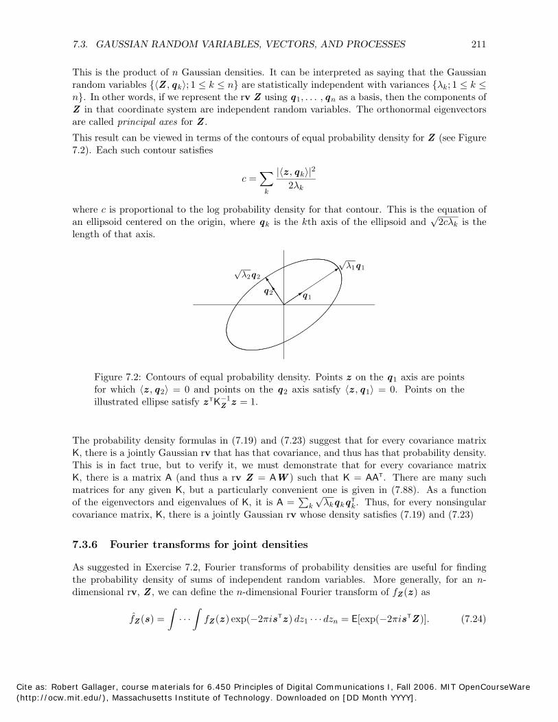
This result can be viewed in terms of the contours of equal probability density for Z (see Figure 7.2). Each such contour satisfies
c = |〈z , qk〉|2
2λkk
where c is proportional to the log probability density for that contour. This is the equation of an ellipsoid centered on the origin, where qk is the kth axis of the ellipsoid and
√2cλk is the
length of that axis.
√λ1q1√
λ2q2
q2 q1
Figure 7.2: Contours of equal probability density. Points z on the q1 axis are points for which 〈z , q2〉 = 0 and points on the q2 axis satisfy 〈z , q1〉 = 0. Points on the illustrated ellipse satisfy z Z z = 1. TK−1
The probability density formulas in (7.19) and (7.23) suggest that for every covariance matrix K, there is a jointly Gaussian rv that has that covariance, and thus has that probability density. This is in fact true, but to verify it, we must demonstrate that for every covariance matrix K, there is a matrix A (and thus a rv Z = AW ) such that K = AAT . There are many such matrices for any given K, but a particularly convenient one is given in (7.88). As a function
Tof the eigenvectors and eigenvalues of K, it is A =
k
√λkqkqk. Thus, for every nonsingular
covariance matrix, K, there is a jointly Gaussian rv whose density satisfies (7.19) and (7.23)
7.3.6 Fourier transforms for joint densities
As suggested in Exercise 7.2, Fourier transforms of probability densities are useful for finding the probability density of sums of independent random variables. More generally, for an n-dimensional rv, Z , we can define the n-dimensional Fourier transform of fZ (z ) as
fZ (s) = fZ (z ) exp(−2πis T dzn = E[exp(−2πis TZ )]. (7.24)· · · z ) dz1 · · ·
Cite as: Robert Gallager, course materials for 6.450 Principles of Digital Communications I, Fall 2006. MIT OpenCourseWare (http://ocw.mit.edu/), Massachusetts Institute of Technology. Downloaded on [DD Month YYYY].
212 CHAPTER 7. RANDOM PROCESSES AND NOISE
If Z is jointly Gaussian, this is easy to calculate. For any given s = 0 , let X = sTZ = k skZk. Thus X is Gaussian with variance E[sTZZ Ts] = sTKZs. From Exercise 7.2,
fX (θ) = E[exp(−2πiθs TZ )] = exp − (2πθ)2
2 sTKZs
. (7.25)
Comparing (7.25) for θ = 1 with (7.24), we see that
fZ (s) = exp − (2π)2s
2
TKZs . (7.26)
The above derivation also demonstrates that fZ (s) is determined by the Fourier transform of each linear combination of the elements of Z . In other words, if an arbitrary rv Z has covariance KZ and has the property that all linear combinations of Z are Gaussian, then the Fourier transform of its density is given by (7.26). Thus, assuming that the Fourier transform of the density uniquely specifies the density, Z must be jointly Gaussian if all linear combinations of Z are Gaussian.
A number of equivalent conditions have now been derived under which a (zero-mean) random vector Z is jointly Gaussian. In summary, each of the following are necessary and sufficient conditions for a rv Z with a nonsingular covariance KZ to be jointly Gaussian.
• Z = AW where the components of W are iid normal and KZ = AAT;
• Z has the joint probability density given in (7.19);
• Z has the joint probability density given in (7.23);
All linear combinations of Z are Gaussian random variables. •
For the case where KZ is singular, the above conditions are necessary and sufficient for any linearly independent subset of the components of Z .
This section has considered only zero-mean random variables, vectors, and processes. The results here apply directly to the fluctuation of arbitrary random variables, vectors, and processes. In particular the probability density for a jointly Gaussian rv Z with a nonsingular covariance matrix KZ and mean vector Z is
1 1 fZ (z ) =
(2π)n/2
det(KZ ) exp −
2(z − Z )TK−
Z 1(z − Z ) . (7.27)
7.4 Linear functionals and filters for random processes
This section defines the important concept of linear functionals on arbitrary random processes Z(t); t ∈ R and then specializes to Gaussian random processes, where the results of the previous section can be used. Assume that the sample functions Z(t, ω) of Z(t) are real L2
waveforms. These sample functions can be viewed as vectors over R in the L2 space of real waveforms. For any given real L2 waveform g(t), there is an inner product,
〈Z(t, ω), g(t)〉 = ∞
Z(t, ω)g(t) dt. −∞
By the Schwarz inequality, the magnitude of this inner product in the space of real L2 functions is upper bounded by ‖Z(t, ω)‖‖g(t)‖ and is thus a finite real value for each ω. This then maps
Cite as: Robert Gallager, course materials for 6.450 Principles of Digital Communications I, Fall 2006. MIT OpenCourseWare (http://ocw.mit.edu/), Massachusetts Institute of Technology. Downloaded on [DD Month YYYY].
7.4. LINEAR FUNCTIONALS AND FILTERS FOR RANDOM PROCESSES 213
sample points ω into real numbers and is thus a random variable,10 denoted V = ∞ Z(t)g(t) dt. −∞
This random variable V is called a linear functional of the process Z(t); t ∈ R. As an example of the importance of linear functionals, recall that the demodulator for both PAM and QAM contains a filter q(t) followed by a sampler. The output of the filter at a sampling time kT for an input u(t) is u(t)q(kT − t) dt. If the filter input also contains additive noise Z(t), then the output at time kT also contains the linear functional Z(t)q(kT − t) dt.
Similarly, for any random process Z(t); t ∈ R (again assuming L2 sample functions) and any real L2 function h(t), consider the result of passing Z(t) through the filter with impulse response h(t). For any L2 sample function Z(t, ω), the filter output at any given time τ is the inner product
〈Z(t, ω), h(τ − t)〉 = ∞
Z(t, ω)h(τ − t) dt. −∞
For each real τ , this maps sample points ω into real numbers and thus (aside from measure theoretic issues),
V (τ) = Z(t)h(τ − t) dt (7.28)
is a rv for each τ . This means that V (τ ); τ ∈ R is a random process. This is called the filtered process resulting from passing Z(t) through the filter h(t). Not much can be said about this general problem without developing a great deal of mathematics, so instead we restrict ourselves to Gaussian processes and other relatively simple examples.
For a Gaussian process, we would hope that a linear functional is a Gaussian random variable. The following examples show that some restrictions are needed even on the class of Gaussian processes.
Example 7.4.1. Let Z(t) = tX for all t ∈ R where X ∼ N (0, 1). The sample functions of this Gaussian process have infinite energy with probability 1. The output of the filter also has infinite energy except except for very special choices of h(t).
Example 7.4.2. For each t ∈ [0, 1], let W (t) be a Gaussian rv, W (t) ∼ N (0, 1). Assume also that E[W (t)W (τ )] = 0 for each t = τ ∈ [0, 1]. The sample functions of this process are discontinuous everywhere11 . We do not have the machinery to decide whether the sample functions are integrable, let alone whether the linear functionals above exist; we come back later to further discuss this example.
In order to avoid the mathematical issues in Example 7.4.2 above, along with a host of other mathematical issues, we start with Gaussian processes defined in terms of orthonormal expansions.
10One should use measure theory over the sample space Ω to interpret these mappings carefully, but this is unnecessary for the simple types of situations here and would take us too far afield.
11Even worse, the sample functions are not measurable. This process would not even be called a random process in a measure theoretic formulation, but it provides an interesting example of the occasional need for a measure theoretic formulation.
Cite as: Robert Gallager, course materials for 6.450 Principles of Digital Communications I, Fall 2006. MIT OpenCourseWare (http://ocw.mit.edu/), Massachusetts Institute of Technology. Downloaded on [DD Month YYYY].
214 CHAPTER 7. RANDOM PROCESSES AND NOISE
7.4.1 Gaussian processes defined over orthonormal expansions
Let φk(t); k ≥ 1 be a countable set of real orthonormal functions and let Zk; k ≥ 1 be a sequence of independent Gaussian random variables, N (0, σ2). Consider the Gaussian process k
defined by
∞Z(t) = Zkφk(t). (7.29)
k=1
Essentially all zero-mean Gaussian processes of interest can be defined this way, although we will not prove this. Clearly a mean can be added if desired, but zero-mean processes are assumed in what follows. First consider the simple case in which σk
2 is nonzero for only finitely many values of k, say 1 ≤ k ≤ n. In this case, Z(t), for each t ∈ R, is a finite sum,
n
Z(t) = Zkφk(t), (7.30) k=1
of independent Gaussian rv’s and thus is Gaussian. It is also clear that Z(t1), Z(t2), . . . Z(t) are jointly Gaussian for all , t1, . . . , t, so Z(t); t ∈ R is in fact a Gaussian random process. The energy in any sample function, z(t) = k zkφk(t) is k
n =1 zk
2 . This is finite (since the sample values are real and thus finite), so every sample function is L2. The covariance function is then easily calculated to be
n
KZ (t, τ) = E[ZkZm]φk(t)φm(τ) = σk 2 φk(t)φk(τ). (7.31)
k,m k=1
Next consider the linear functional Z(t)g(t) dt where g(t) is a real L2 function, n ∞ ∞V = Z(t)g(t) dt = Zk φk(t)g(t) dt. (7.32)
k=1−∞ −∞
Since V is a weighted sum of the zero-mean independent Gaussian rv’s Z1, . . . , Zn, V is also Gaussian with variance
n
σV 2 = E[V 2] = σk
2|〈φk, g〉|2 . (7.33) k=1
Next consider the case where n is infinite but σ2 < ∞. The sample functions are still L2 (atk k least with probability 1). Equations (7.29), (7.30), (7.31), (7.32) and (7.33) are still valid, and Z is still a Gaussian rv. We do not have the machinery to easily prove this, although Exercise 7.7 provides quite a bit of insight into why these results are true.
Finally, consider a finite set of L2 waveforms gm(t); 1 ≤ m ≤ . Let Vm = ∞ Z(t)gm(t) dt. −∞
By the same argument as above, Vm is a Gaussian rv for each m. Furthermore, since each linear combination of these variables is also a linear functional, it is also Gaussian, so V1, . . . , V is jointly Gaussian.
Cite as: Robert Gallager, course materials for 6.450 Principles of Digital Communications I, Fall 2006. MIT OpenCourseWare (http://ocw.mit.edu/), Massachusetts Institute of Technology. Downloaded on [DD Month YYYY].
7.4. LINEAR FUNCTIONALS AND FILTERS FOR RANDOM PROCESSES 215
7.4.2 Linear filtering of Gaussian processes
We can use the same argument as in the previous subsection to look at the output of a linear filter for which the input is a Gaussian process Z(t); t ∈ R. In particular, assume that Z(t) = k Zkφk(t) where Z1, Z2, . . . is an independent sequence Zk ∼ N (0, σk
2 satisfying σ2 < ∞ and where φ1(t), φ2(t), . . . , is a sequence of orthonormal functions. k k
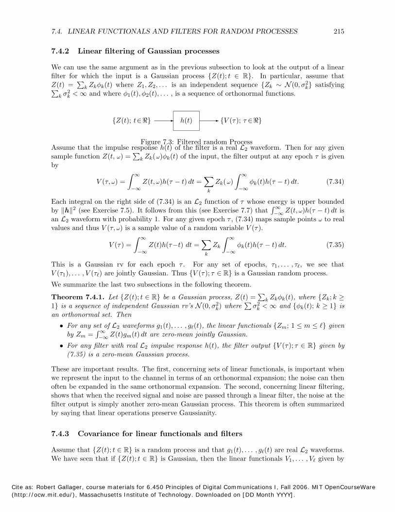
Z(t); t∈ h(t) V (τ); τ ∈
Figure 7.3: Filtered random ProcessAssume that the impulse response h(t) of the filter is a real L2 waveform. Then for any given sample function Z(t, ω) = k Zk(ω)φk(t) of the input, the filter output at any epoch τ is given by
∞ ∞V (τ, ω) = Z(t, ω)h(τ − t) dt = Zk(ω) φk(t)h(τ − t) dt. (7.34)
k−∞ −∞
Each integral on the right side of (7.34) is an L2 function of τ whose energy is upper bounded by ‖h‖2 (see Exercise 7.5). It follows from this (see Exercise 7.7) that ∞
Z(t, ω)h(τ − t) dt is −∞an L2 waveform with probability 1. For any given epoch τ , (7.34) maps sample points ω to real values and thus V (τ, ω) is a sample value of a random variable V (τ).
∞ ∞V (τ) = Z(t)h(τ−t) dt = Zk φk(t)h(τ − t) dt. (7.35)
k−∞ −∞
This is a Gaussian rv for each epoch τ . For any set of epochs, τ1, . . . , τ, we see that V (τ1), . . . , V (τ) are jointly Gaussian. Thus V (τ); τ ∈ R is a Gaussian random process.
We summarize the last two subsections in the following theorem.
Theorem 7.4.1. Let Z(t); t ∈ R be a Gaussian process, Z(t) = Zkφk(t), where Zk; k ≥ k 1 is a sequence of independent Gaussian rv’s N (0, σ2) where σ2 < ∞ and φk(t); k ≥ 1 isk k an orthonormal set. Then
• For any set of L2 waveforms g1(t), . . . , g(t), the linear functionals Zm; 1 ≤ m ≤ given by Zm = ∞
Z(t)gm(t) dt are zero-mean jointly Gaussian. −∞For any filter with real L2 impulse response h(t), the filter output V (τ); τ ∈ R given by • (7.35) is a zero-mean Gaussian process.
These are important results. The first, concerning sets of linear functionals, is important when we represent the input to the channel in terms of an orthonormal expansion; the noise can then often be expanded in the same orthonormal expansion. The second, concerning linear filtering, shows that when the received signal and noise are passed through a linear filter, the noise at the filter output is simply another zero-mean Gaussian process. This theorem is often summarized by saying that linear operations preserve Gaussianity.
7.4.3 Covariance for linear functionals and filters
Assume that Z(t); t ∈ R is a random process and that g1(t), . . . , g(t) are real L2 waveforms. We have seen that if Z(t); t ∈ R is Gaussian, then the linear functionals V1, . . . , V given by
Cite as: Robert Gallager, course materials for 6.450 Principles of Digital Communications I, Fall 2006. MIT OpenCourseWare (http://ocw.mit.edu/), Massachusetts Institute of Technology. Downloaded on [DD Month YYYY].
216 CHAPTER 7. RANDOM PROCESSES AND NOISE
Vm = ∞ Z(t)gm(t) dt are jointly Gaussian for 1 ≤ m ≤ . We now want to find the covariance −∞
for each pair Vj , Vm of these random variables. The result does not depend on the process Z(t) being Gaussian. The computation is quite simple, although we omit questions of limits, interchanges of order of expectation and integration, etc. A more careful derivation could be made by returning to the sampling theorem arguments before, but this would somewhat obscure the ideas. Assuming that the process Z(t) is zero mean,
∞ ∞E[Vj Vm] = E Z(t)gj (t) dt Z(τ)gm(τ ) dτ (7.36) −∞ −∞
= ∞ ∞
gj (t)E[Z(t)Z(τ )]gm(τ ) dt dτ (7.37) t=−∞ τ =−∞∞ ∞
= gj (t)KZ (t, τ )gm(τ) dt dτ. (7.38) t=−∞ τ =−∞
Each covariance term (including E[Vm2 ] for each m) then depends only on the covariance function
of the process and the set of waveforms gm; 1 ≤ m ≤ . The convolution V (r) = Z(t)h(r − t) dt is a linear functional at each time r, so the covariance for the filtered output of Z(t); t ∈ R follows in the same way as the results above. The output V (r) for a filter with a real L2 impulse response h is given by (7.35), so the covariance of the output can be found as
KV (r, s) = E[V (r)V (s)]
= E ∞
Z(t)h(r−t)dt ∞
Z(τ )h(s−τ)dτ −∞ −∞
= ∞ ∞
h(r−t)KZ (t, τ )h(s−τ)dtdτ. (7.39) −∞ −∞
7.5 Stationarity and related concepts
Many of the most useful random processes have the property that the location of the time origin is irrelevant, i.e., they “behave” the same way at one time as at any other time. This property is called stationarity and such a process is called a stationary process.
Since the location of the time origin must be irrelevant for stationarity, random processes that are defined over any interval other than (−∞, ∞) cannot be stationary. Thus assume a process that is defined over (−∞, ∞).
The next requirement for a random process Z(t); t ∈ R to be stationary is that Z(t) must be identically distributed for all epochs t ∈ R. This means that, for any epochs t and t + τ , and for any real number x, PrZ(t) ≤ x = PrZ(t + τ) ≤ x. This does not mean that Z(t) and Z(t + τ ) are the same random variables; for a given sample outcome ω of the experiment, Z(t, ω) is typically unequal to Z(t+τ, ω). It simply means that Z(t) and Z(t+τ ) have the same distribution function, i.e.,
FZ(t)(x) = FZ(t+τ)(x) for all x. (7.40)
This is still not enough for stationarity, however. The joint distributions over any set of epochs must remain the same if all those epochs are shifted to new epochs by an arbitrary shift τ . This includes the previous requirement as a special case, so we have the definition:
Cite as: Robert Gallager, course materials for 6.450 Principles of Digital Communications I, Fall 2006. MIT OpenCourseWare (http://ocw.mit.edu/), Massachusetts Institute of Technology. Downloaded on [DD Month YYYY].

7.5. STATIONARITY AND RELATED CONCEPTS 217
Definition 7.5.1. A random process Z(t); t∈R is stationary if, for all positive integers , for all sets of epochs t1, . . . , t ∈ R, for all amplitudes z1, . . . , z, and for all shifts τ ∈ R,
FZ(t1),... ,Z(t)(z1 . . . , z) = FZ(t1+τ),... ,Z(t+τ )(z1 . . . , z). (7.41)
For the typical case where densities exist, this can be rewritten as
fZ(t1),... ,Z(t)
(z1 . . . , z) = fZ(t1+τ ),... ,Z(t+τ )
(z1 . . . , z) (7.42)
for all z1, . . . , z ∈ R.
For a (zero-mean) Gaussian process, the joint distribution of Z(t1), . . . , Z(t) depends only on the covariance of those variables. Thus, this distribution will be the same as that of Z(t1+τ), . . . , Z(t+τ) if KZ (tm, tj ) = KZ (tm+τ, tj +τ) for 1 ≤ m, j ≤ . This condition will be satisfied for all τ , all , and all t1, . . . , t (verifying that Z(t) is stationary) if KZ (t1, t2) = KZ (t1+τ, t2+τ) for all τ and all t1, t2. This latter condition will be satisfied if KZ (t1, t2) = KZ (t1−t2, 0) for all t1, t2. We have thus shown that a zero-mean Gaussian process is stationary if
KZ (t1, t2) = KZ (t1−t2, 0) for all t1, t2 ∈ R. (7.43)
Conversely, if (7.43) is not satisfied for some choice of t1, t2, then the joint distribution of Z(t1), Z(t2) must be different from that of Z(t1−t2), Z(0), and the process is not stationary. The following theorem summarizes this.
Theorem 7.5.1. A zero-mean Gaussian process Z(t); t∈R is stationary if and only if (7.43) is satisfied.
An obvious consequence of this is that a Gaussian process with a nonzero mean is stationary if and only if its mean is constant and its fluctuation satisfies (7.43).
7.5.1 Wide-sense stationary (WSS) random processes
There are many results in probability theory that depend only on the covariances of the random variables of interest (and also the mean if nonzero). For random processes, a number of these classical results are simplified for stationary processes, and these simplifications depend only on the mean and covariance of the process rather than full stationarity. This leads to the following definition:
Definition 7.5.2. A random process Z(t); t∈ is wide-sense stationary (WSS) if E[Z(t1)] = E[Z(0)] and KZ (t1, t2) = KZ (t1−t2, 0) for all t1, t2 ∈ R.
Since the covariance function KZ (t+τ, t) of a WSS process is a function of only one variable τ , we will often write the covariance function as a function of one variable, namely KZ (τ) in place of KZ (t+τ, t). In other words, the single variable in the single argument form represents the difference between the two arguments in two argument form. Thus for a WSS process, KZ (t, τ) = KZ (t−τ, 0) = KZ (t − τ).
The random processes defined as expansions of T -spaced sinc functions have been discussed several times. In particular let
V (t) = Vk sinc t − kT
, (7.44)T
k
Cite as: Robert Gallager, course materials for 6.450 Principles of Digital Communications I, Fall 2006. MIT OpenCourseWare (http://ocw.mit.edu/), Massachusetts Institute of Technology. Downloaded on [DD Month YYYY].
218 CHAPTER 7. RANDOM PROCESSES AND NOISE
where . . . , V−1, V0, V1, . . . is a sequence of (zero-mean) iid rv’s. As shown in 7.8, the covariance function for this random process is
KV (t, τ) = σV 2 sinc
t − kT sinc
τ − kT , (7.45)
T T k
where σV 2 is the variance of each Vk. The sum in (7.45), as shown below, is a function only of
t − τ , leading to the theorem:
Theorem 7.5.2 (Sinc expansion). The random process in (7.44) is WSS. In addition, if the rv’s Vk; k ∈ Z are iid Gaussian, the process is stationary. The covariance function is given by
KV(t − τ) = σ2 sinc t − τ
. (7.46)V T
Proof: From the sampling theorem, any L2 function u(t), baseband limited to 1/(2T ), can be expanded as
u(t) = u(kT )sinc t − kT
. (7.47)T
k
For any given τ , take u(t) to be sinc( t−T
τ ). Substituting this in (7.47),
sinc t−τ
=
sinc kT−τ
sinc t−kT
=
sinc τ−kT
sinc t−kT
. (7.48)T T T T T
k k
Substituting this in (7.45) shows that the process is WSS with the stated covariance. As shown in subsection 7.4.1, V (t); t ∈ R is Gaussian if the rv’s Vk are Gaussian. From Theorem 7.5.1, this Gaussian process is stationary since it is WSS.
Next consider another special case of the sinc expansion in which each Vk is binary, taking values ±1 with equal probability. This corresponds to a simple form of a PAM transmitted waveform. In this case, V (kT ) must be ±1, whereas for values of t between the sample points, V (t) can take on a wide range of values. Thus this process is WSS but cannot be stationary. Similarly, any discrete distribution for each Vk creates a process that is WSS but not stationary.
There are not many important models of noise processes that are WSS but not stationary12 , despite the above example and the widespread usage of the term WSS. Rather, the notion of wide-sense stationarity is used to make clear, for some results, that they depend only on the mean and covariance, thus perhaps making it easier to understand them.
The Gaussian sinc expansion brings out an interesting theoretical nonsequitur. Assuming that σV
2 > 0, i.e., that the process is not the trivial process for which V (t) = 0 with probability 1 for all t, the expected energy in the process (taken over all time) is infinite. It is not difficult to convince oneself that the sample functions of this process have infinite energy with probability 1. Thus stationary noise models are simple to work with, but the sample functions of these processes don’t fit into the L2 theory of waveforms that has been developed. Even more important than the issue of infinite energy, stationary noise models make unwarranted assumptions about the
12An important exception is interference from other users, which as the above sinc expansion with binary samples shows, can be WSS but not stationary. Even in this case, if the interference is modeled as just part of the noise (rather than specifically as interference), the nonstationarity is usually ignored.
Cite as: Robert Gallager, course materials for 6.450 Principles of Digital Communications I, Fall 2006. MIT OpenCourseWare (http://ocw.mit.edu/), Massachusetts Institute of Technology. Downloaded on [DD Month YYYY].
7.5. STATIONARITY AND RELATED CONCEPTS 219
very distant past and future. The extent to which these assumptions affect the results about the present is an important question that must be asked.
The problem here is not with the peculiarities of the Gaussian sinc expansion. Rather it is that stationary processes have constant power over all time, and thus have infinite energy. One practical solution13 to this is simple and familiar. The random process is simply truncated in any convenient way. Thus, when we say that noise is stationary, we mean that it is stationary within a much longer time interval than the interval of interest for communication. This is not very precise, and the notion of effective stationarity is now developed to formalize this notion of a truncated stationary process.
7.5.2 Effectively stationary and effectively WSS random processes
T TDefinition 7.5.3. A (zero-mean) random process is effectively stationary within [−joint probability assignment for t1, . . . , tn is the same as that for t1+τ, t2+τ, . . . , tn+τ whenever
] if the0 0 2 , 2
T0 Tand t1+τ, t2+τ, . . . , tn+τ are all contained in the interval [− ]. It is effectively0t1, . . . , tn 2 , 2 T T T T] if KZ (t, τ) is a function only of t − τ for t, τ ∈ [−2 , 2 2 , 2
process with nonzero mean is effectively stationary (effectively WSS) if its mean is constant WSS within [− ]. A random0 0 0 0
T T T Twithin [− ] and its fluctuation is effectively stationary (WSS) within [− ].0 0 0 0 2 , 2 ,2 2
One way to view a stationary (WSS) random process is in the limiting sense of a process that isT Teffectively stationary (WSS) for all intervals [−
and filtering, the nature of this limit as T0 becomes large is quite simple and natural, whereas ]. For operations such as linear functionals0 0
2 , 2
for frequency domain results, the effect of finite T0 is quite subtle. T T T T
00
For an effectively WSS process within [−of a single parameter, KZ (t, τ) = KZ (t − τ) for t, τ ∈ [− 00
], the covariance within [−2 , 2 2 , 2 ] is a function0 0 0 0
T T ]. Note however that t − τ can ).
2 , 2 T T T Trange from −T0 (for t= ) to T0 (for t=0 0, τ= , τ=− −2 2 2 2
T0 T0
point where t − τ = −T00 2
T
τ
line where t − τ = −T0 2
line where t − τ = 0
line where t − τ = T0 2
3line where t − τ =0T
−
T0− 42
t2 2
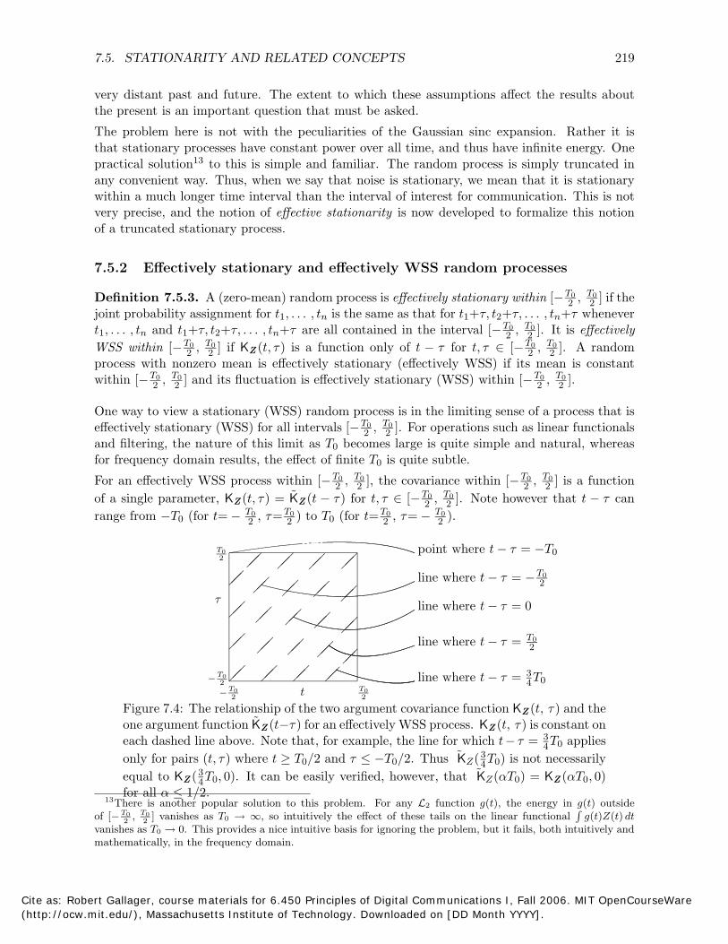
Figure 7.4: The relationship of the two argument covariance function KZ (t, τ) and the one argument function KZ (t−τ) for an effectively WSS process. KZ (t, τ) is constant on each dashed line above. Note that, for example, the line for which t− τ = 3T0 applies4
only for pairs (t, τ) where t ≥ T0/2 and τ ≤ −T0/2. Thus KZ (3T0) is not necessarily4
equal to KZ (34T0, 0). It can be easily verified, however, that KZ (αT0) = KZ (αT0, 0)
for all α ≤ 1/2. 13There is another popular solution to this problem. For any L
, so intuitively the effect of these tails on the linear functional function g(t), the energy in g(t) outside2
00T T
vanishes as T0 0. This provides a nice intuitive basis for ignoring the problem, but it fails, both intuitively and→mathematically, in the frequency domain.
Cite as: Robert Gallager, course materials for 6.450 Principles of Digital Communications I, Fall 2006. MIT OpenCourseWare (http://ocw.mit.edu/), Massachusetts Institute of Technology. Downloaded on [DD Month YYYY].
of [− ] vanishes as T0 g(t)Z(t) dt→ ∞,2 2
220 CHAPTER 7. RANDOM PROCESSES AND NOISE
Since a Gaussian process is determined by its covariance function and mean, it is effectively stationary within [− 2 ] if it is effectively WSS.T T
2 ,
Note that the difference between a stationary and effectively stationary random process for large T0 is primarily a difference in the model and not in the situation being modeled. If two models have a significantly different behavior over the time intervals of interest, or more concretely, if noise in the distant past or future has a significant effect, then the entire modeling issue should be rethought.
7.5.3 Linear functionals for effectively WSS random processes
The covariance matrix for a set of linear functionals and the covariance function for the output of a linear filter take on simpler forms for WSS or effectively WSS processes than the corresponding forms for general processes derived in Subsection 7.4.3.
Let Z(t) be a zero-mean WSS random process with covariance function KZ (t − τ) for t, τ ∈
00
T2 , 0 T
2 0 00] and let g1(t), g2(t), . . . , g(t) be a set of L2 functions nonzero only within [−T
2 , T
be given by [− ].2 For the conventional WSS case, we can take T0 = ∞. Let the linear functional Vm T0/2
Z(t)gm(t) dt for 1 ≤ m ≤ . The covariance E[VmVj ] is then given by −T0/2
T
0
0
E[VmVj ] = E Z(t)gm(t) dt T
∞2
Z(τ )gj (τ) dτ − −∞
2
0
0
0
0T T
= gmT T
22
(t)KZ (t−τ)gj (τ) dτ dt. (7.49) − −
2 2
0Note that this depends only on the covariance where t, τ ∈ [−T2 ,
effectively WSS. This is not surprising, since we would not expect Vm
0T ], i.e., where Z(t) is to depend on the behavior 2
of the process outside of where gm(t) is nonzero.
7.5.4 Linear filters for effectively WSS random processes
Next consider passing a random process Z(t); t ∈ R through a linear time-invariant filter whose impulse response h(t) is L2. As pointed out in 7.28, the output of the filter is a random process V (τ); τ ∈ R given by
V (τ) = ∞
Z(t1)h(τ −t1) dt1. −∞
Note that V (τ) is a linear functional for each choice of τ . The covariance function evaluated at t, τ is the covariance of the linear functionals V (t) and V (τ ). Ignoring questions of orders of integration and convergence,
KV (t, τ) = ∞ ∞
h(t−t1)KZ (t1, t2)h(τ −t2)dt1dt2. (7.50) −∞ −∞
First assume that Z(t); t ∈ R is WSS in the conventional sense. Then KZ (t1, t2) can be replaced by KZ (t1−t2). Replacing t1−t2 by s (i.e., t1 by t2 + s),
KV (t, τ ) = ∞ ∞
h(t−t2−s)KZ (s) ds h(τ−t2) dt2. −∞ −∞
Cite as: Robert Gallager, course materials for 6.450 Principles of Digital Communications I, Fall 2006. MIT OpenCourseWare (http://ocw.mit.edu/), Massachusetts Institute of Technology. Downloaded on [DD Month YYYY].

7.5. STATIONARITY AND RELATED CONCEPTS 221
Replacing t2 by τ+µ,
KV (t, τ) = ∞ ∞
h(t−τ −µ−s)KZ (s) ds h(−µ) dµ. (7.51) −∞ −∞
Thus KV (t, τ ) is a function only of t−τ . This means that V (t); t ∈ R is WSS. This is not surprising; passing a WSS random process through a linear time-invariant filter results in another WSS random process.
If Z(t); t ∈ R is a Gaussian process, then, from Theorem 7.4.1, V (t); t ∈ R is also a Gaussian process. Since a Gaussian process is determined by its covariance function, it follows that if Z(t) is a stationary Gaussian process, then V (t) is also a stationary Gaussian process.
We do not have the mathematical machinery to carry out the above operations carefully over the infinite time interval14 . Rather, it is now assumed that Z(t); t ∈ R is effectively WSS
]. It will also be assumed that the impulse response h(t) above is time-limited within [−T T
in the sense that for some finite A, h(t) = 0 for
00 2 , 2
|t| > A.
0
00
0
tions that are L2 within [−T T ] with probability 1. Let Z(t) be the input to a filter with an L2
T TLet ( ); be effectively WSS within [Theorem 7.5.3. RZ t t ∈ − ,2
T. Then for R→ T] and its sample functions within [0 A− −2
00
] and have sample func2
2 , 2
time-limited impulse response h(t); [−A, A] V (t); t ∈ R is WSS within [−T +A, T
are L2 with probability 1.
0
> A, the output random process2 0+A, T2 −A]2 2
0
0
within [−T2 ,
T +A, T
0T2 ]. Let
00
Proof: Let z(t) be a sample function of Z(t) and assume z(t) is L2
v(τ ) = z(t)h(τ − t) dt be the corresponding filter output. For each τ ∈ [−T T2 ,
0 2 −A], v(τ )
]. Thus, if we replace z(t) by z0(t) = z(t)rect[T0], 2
is determined by z(t) in the range t ∈ [− 2 00the filter output, say v0(τ) will equal v(τ) for τ ∈ [−T2 −A]. The time-limited function
z0(t) is L1 as well as L2. This implies that the Fourier transform z0(f) is bounded, say by z0(f) ≤ B, for each f . Since v0(f) = z0(f)h(f), we see that
2|v0(f)|2 df = |z0(f)| |h(f)|2 df ≤ B2 |h(f)|2 df < ∞
+A, T2
0
0
00
00
v0(f), and thus also v0(t), is L2. Now v0(t), when truncated to [−T
is equal to v(t) truncated to [−T2 −A], so the truncated version of v(t) is L2.
sample functions of V (t), truncated to [−T2 −A], are L2 with probability 1.
T
+A, TThis means that ˆ 0 2 −A]
Thus the 2
+A, T2
+A, T2
0TFinally, since ( ); can be truncated to [RZ t t ∈ −00
2 , that KZ (t1, t2) can be truncated to t1, t2 ∈ [−T
2 , T
becomes
] with no lack of generality, it follows2 0T2
0+A, T2 −A], (7.50) ]. Thus, for t, τ ∈ [−2
0 2
0 2
T T
h(t−t1)KZ (t1−t2)h(τ −t2)dt1dt2.KV (t, τ) = (7.52)0 2
T − 0 2
T−
0T2
0+A, T2 −A].The argument in (7.50, 7.51) shows that V (t) is effectively WSS within [−
The above theorem, along with the effective WSS result about linear functionals, shows us that results about WSS processes can be used within finite intervals. The result in the theorem about
14More important, we have no justification for modeling a process over the infinite time interval. Later, however, after building up some intuition about the relationship of an infinite interval to a very large interval, we can use the simpler equations corresponding to infinite intervals.
Cite as: Robert Gallager, course materials for 6.450 Principles of Digital Communications I, Fall 2006. MIT OpenCourseWare (http://ocw.mit.edu/), Massachusetts Institute of Technology. Downloaded on [DD Month YYYY].
222 CHAPTER 7. RANDOM PROCESSES AND NOISE
the interval of effective stationarity being reduced by filtering should not be too surprising. If we truncate a process, and then pass it through a filter, the filter spreads out the effect of the truncation. For a finite duration filter, however, as assumed here, this spreading is limited.
The notion of stationarity (or effective stationarity) makes sense as a modeling tool where T0
above is very much larger than other durations of interest, and in fact where there is no need for explicit concern about how long the process is going to be stationary.
The above theorem essentially tells us that we can have our cake and eat it too. That is, transmitted waveforms and noise processes can be truncated, thus making use of both common sense and L2 theory, but at the same time insights about stationarity can still be relied upon. More specifically, random processes can be modeled as stationary, without specifying a specific interval [−T
2 , T
asymptotic versions of finite duration processes.
00 2 ] of effective stationarity, because stationary processes can now be viewed as
Appendices 7A.2 and 7A.3 provide a deeper analysis of WSS processes truncated to an interval. The truncated process is represented as a Fourier series with random variables as coefficients. This gives a clean interpretation of what happens as the interval size is increased without bound, and also gives a clean interpretation of the effect of time-truncation in the frequency domain. Another approach to a truncated process is the Karhunen-Loeve expansion, which is discussed in 7A.4.
7.6 Stationary and WSS processes in the Frequency Domain
Stationary and WSS zero-mean processes, and particularly Gaussian processes, are often viewed more insightfully in the frequency domain than in the time domain. An effectively WSS process over [−T T
process can be viewed as a process that is effectively WSS for each T0.
00 2 , 2 ] has a single variable covariance function KZ (τ ) defined over [T0, T0]. A WSS
The energy in such aprocess, truncated to [− 00T T
2 , defined over a larger and larger interval as T0 → ∞. Assume in what follows that this limiting covariance is L2. This does not appear to rule out any but the most pathological processes.
First we look at linear functionals and linear filters, ignoring limiting questions and convergence issues and assuming that T0 is ‘large enough’. We will refer to the random processes as stationary, while still assuming L2 sample functions.
For a zero-mean WSS process Z(t); t ∈ R and a real L2 function g(t), consider the linear functional V = g(t)Z(t) dt. From (7.49),
E[V 2] = ∞
g(t) ∞
KZ (t − τ )g(τ) dτ dt (7.53) −∞ −∞ =
∞
g(t) KZ ∗ g (t) dt. (7.54) −∞
where KZ ∗g denotes the convolution of the waveforms KZ (t) and g(t). Let SZ (f) be the Fourier transform of KZ (t). The function SZ (f) is called the spectral density of the stationary process Z(t); t ∈ R. Since KZ (t) is L2, real, and symmetric, its Fourier transform is also L2, real, and symmetric, and, as shown later, SZ (f) ≥ 0. It is also shown later that SZ (f) at each frequency f can be interpreted as the power per unit frequency at f .
Let θ(t) = [KZ ∗ g ](t) be the convolution of KZ and g . Since g and KZ are real, θ(t) is also real
2 ], is linearly increasing in T0, but the covariance simply becomes
Cite as: Robert Gallager, course materials for 6.450 Principles of Digital Communications I, Fall 2006. MIT OpenCourseWare (http://ocw.mit.edu/), Massachusetts Institute of Technology. Downloaded on [DD Month YYYY].

7.6. STATIONARY AND WSS PROCESSES IN THE FREQUENCY DOMAIN 223
so θ (t ) = θ ∗(t ). Using Parseval’s theorem for Fourier transforms,
E[V 2] = ∞
g (t )θ ∗(t ) dt = ∞
g(f )θ∗(f ) df. −∞ −∞
Since θ (t ) is the convolution of KZ and g , we see that θ(f ) = S Z (f )g (f ). Thus,
E[V 2] = ∞
g(f )S Z (f )g ∗(f ) df = ∞
|g(f )| 2 S Z (f ) df. (7.55) −∞ −∞
Note that E[V 2] ≥ 0 and that this holds for all real L2 functions g (t ). The fact that g (t ) is real constrains the transform g (f ) to satisfy g (f ) = g ∗(−f ), and thus |g(f )| = |g(−f )| for all f . Subject to this constraint and the constraint that |g(f )| be L2, |g(f )| can be chosen as any L2
function. Stated another way, g (f ) can be chosen arbitrarily for f ≥ 0 subject to being L2.
Since S Z (f ) = S Z (−f ), (7.55) can be rewritten as
E[V 2] = 0
∞
2 |g(f )| 2 S Z (f ) df.
Since E[V 2] ≥ 0 and |g(f )| is arbitrary, it follows that S Z (f ) ≥ 0 for all f ∈ R.
The conclusion here is that the spectral density of any WSS random process must be nonnegative. Since S Z (f ) is also the Fourier transform of K(t ), this means that a necessary property of any single variable covariance function is that it have a nonnegative Fourier transform.
Next, let V m = g m(t )Z (t ) dt where the function g m(t ) is real and L2 for m = 1, 2. From (7.49),
E[V 1V 2] = ∞
g 1(t ) ∞
KZ (t − τ )g 2(τ ) dτ dt (7.56) −∞ −∞ =
∞
g 1(t ) K ∗ g2 (t ) dt. (7.57) −∞
Let g m(f ) be the Fourier transform of g m(t ) for m = 1, 2, and let θ (t ) = [KZ (t ) ∗ g2](t ) be the convolution of KZ and g2. Let θ(f ) = S Z (f )g 2(f ) be its Fourier transform. As before, we have
E[V 1V 2] = g1(f )θ∗(f ) df = g1(f )S Z (f )g 2∗(f ) df. (7.58)
There is a remarkable feature in the above expression. If g 1(f ) and g 2(f ) have no overlap in frequency, then E[V 1V 2] = 0. In other words, for any stationary process, two linear functionals over different frequency ranges must be uncorrelated. If the process is Gaussian, then the linear functionals are independent. This means in essence that Gaussian noise in different frequency bands must be independent. That this is true simply because of stationarity is surprising. Appendix 7A.3 helps to explain this puzzling phenomenon, especially with respect to effective stationarity.
Next, let φ m(t ); m ∈ Z be a set of real orthonormal functions and let φm(f ) be the corresponding set of Fourier transforms. Letting V m = Z (t )φ m(t ) dt , (7.58) becomes
E[V mV j ] = φm(f )S Z (f )φj∗(f ) df. (7.59)
Cite as: Robert Gallager, course materials for 6.450 Principles of Digital Communications I, Fall 2006. MIT OpenCourseWare (http://ocw.mit.edu/), Massachusetts Institute of Technology. Downloaded on [DD Month YYYY].

224 CHAPTER 7. RANDOM PROCESSES AND NOISE
If the set of orthonormal functions φm(t); m ∈ Z is limited to some frequency band, and if SZ (f) is constant, say with value N0/2 in that band, then
E[VmVj ] = N0/2 φm(f)φ∗j (f) df. (7.60)
By Parseval’s theorem for Fourier transforms, we have
φm(f)φ∗j (f) df = δmj , and thus
E[VmVj ] = N0
δmj . (7.61)2
The rather peculiar looking constant N0/2 is explained in the next section. For now, however, it is possible to interpret the meaning of the spectral density of a noise process. Suppose that SZ (f) is continuous and approximately constant with value SZ (fc) over some narrow band of frequencies around fc and suppose that φ1(t) is constrained to that narrow band. Then the variance of the linear functional ∞
Z(t)φ1(t) dt is approximately SZ (fc). In other words, −∞SZ (fc) in some fundamental sense describes the energy in the noise per degree of freedom at the frequency fc. The next section interprets this further.
7.7 White Gaussian noise
Physical noise processes are very often reasonably modeled as zero mean, stationary, and Gaussian. There is one further simplification that is often reasonable. This is that the covariance between the noise at two epochs dies out very rapidly as the interval between those epochs increases. The interval over which this covariance is significantly nonzero is often very small relative to the intervals over which the signal varies appreciably. This means that the covariance function KZ (τ) looks like a short-duration pulse around τ = 0.
We know from linear system theory that
KZ (t − τ)g(τ )dτ is equal to g(t) if KZ (t) is a unit impulse. Also, this integral is approximately equal to g(t) if KZ (t) has unit area and is a narrow pulse relative to changes in g(t). It follows that under the same circumstances, (7.56) becomes
E[V1V2 ∗] = g1(t)KZ (t − τ )g2(τ) dτ dt ≈ g1(t)g2(t) dt. (7.62)
t τ
This means that if the covariance function is very narrow relative to the functions of interest, then its behavior relative to those functions is specified by its area. In other words, the covariance function can be viewed as an impulse of a given magnitude. We refer to a zero-mean WSS Gaussian random process with such a narrow covariance function as White Gaussian Noise (WGN). The area under the covariance function is called the intensity or the spectral density of the WGN and is denoted by the symbol N0/2. Thus, for L2 functions g1(t), g2(t), . . . in the range of interest, and for WGN (denoted by W (t); t ∈ R) of intensity N0/2, the random variable Vm = W (t)gm(t) dt has the variance
2E[Vm2 ] = (N0/2) gm(t) dt. (7.63)
Similarly, the random variables Vj and Vm have the covariance
E[Vj Vm] = (N0/2) gj (t)gm(t) dt. (7.64)
Cite as: Robert Gallager, course materials for 6.450 Principles of Digital Communications I, Fall 2006. MIT OpenCourseWare (http://ocw.mit.edu/), Massachusetts Institute of Technology. Downloaded on [DD Month YYYY].
7.7. WHITE GAUSSIAN NOISE 225
Also V1, V2, . . . are jointly Gaussian.
The most important special case of (7.63) and (7.64) is to let φj(t) be a set of orthonormalfunctions and let W (t) be WGN of intensity N0/2. Let Vm = φm(t)W (t) dt. Then, from (7.63) and (7.64),
E[VjVm] = (N0/2)δjm. (7.65)
This is an important equation. It says that if the noise can be modeled as WGN, then when the noise is represented in terms of any orthonormal expansion, the resulting random variables are iid. Thus, we can represent signals in terms of an arbitrary orthonormal expansion, and represent WGN in terms of the same expansion, and the result is iid Gaussian random variables.
Since the coefficients of a WGN process in any orthonormal expansion are iid Gaussian, it is common to also refer to a random vector of iid Gaussian rv’s as WGN.
If KW (t) is approximated by (N0/2)δ(t), then the spectral density is approximated by SW (f) = N0/2. If we are concerned with a particular band of frequencies, then we are interested in SW (f) being constant within that band, and in this case, W (t); t ∈ R can be represented as white noise within that band. If this is the only band of interest, we can model15 SW (f) as equal to N0/2 everywhere, in which case the corresponding model for the covariance function is (N0/2)δ(t).
The careful reader will observe that WGN has not really been defined. What has been said, in essence, is that if a stationary zero-mean Gaussian process has a covariance function that is very narrow relative to the variation of all functions of interest, or a spectral density that is constant within the frequency band of interest, then we can pretend that the covariance function is an impulse times N0/2, where N0/2 is the value of SW (f) within the band of interest. Unfortunately, according to the definition of random process, there cannot be any Gaussian random process W (t) whose covariance function is K(t) = (N0/2)δ(t). The reason for this dilemma is that E[W 2(t)] = KW (0). We could interpret KW (0) to be either undefined or ∞, but either way, W (t) cannot be a random variable (although we could think of it taking on only the values plus or minus ∞).
Mathematicians view WGN as a generalized random process, in the same sense as the unit impulse δ(t) is viewed as a generalized function. That is, the impulse function δ(t) is not viewed as an ordinary function taking the value 0 for t = 0 and the value ∞ at t = 0. Rather, it is viewed in terms of its effect on other, better behaved, functions g(t), where ∞
g(t)δ(t) dt = g(0). In −∞the same way, WGN is not viewed in terms of random variables at each epoch of time. Rather it is viewed as a generalized zero-mean random process for which linear functionals are jointly Gaussian, for which variances and covariances are given by (7.63) and (7.64), and for which the covariance is formally taken to be (N0/2)δ(t).
Engineers should view WGN within the context of an overall bandwidth and time interval of interest, where the process is effectively stationary within the time interval and has a constant spectral density over the band of interest. Within that context, the spectral density can be viewed as constant, the covariance can be viewed as an impulse, and (7.63) and (7.64) can be used.
The difference between the engineering view and the mathematical view is that the engineering view is based on a context of given time interval and bandwidth of interest, whereas the math
15This is not at obvious as it sounds, and will be further discussed in terms of the theorem of irrelevance in the next chapter.
Cite as: Robert Gallager, course materials for 6.450 Principles of Digital Communications I, Fall 2006. MIT OpenCourseWare (http://ocw.mit.edu/), Massachusetts Institute of Technology. Downloaded on [DD Month YYYY].
226 CHAPTER 7. RANDOM PROCESSES AND NOISE
ematical view is based on a very careful set of definitions and limiting operations within which theorems can be stated without explicitly defining the context. Although the ability to prove theorems without stating the context is valuable, any application must be based on the context.
7.7.1 The sinc expansion as an approximation to WGN
Theorem 7.5.2 treated the process Z(t) = Zksinc t−kT where each rv Zk; k ∈ Z is iid k T and N (0, σ2). We found that the process is zero-mean Gaussian and stationary with covariance function KZ (t − τ) = σ2sinc( t−τ ). The spectral density for this process is then given by T
SZ (f) = σ2T rect(fT ). (7.66)
This process has a constant spectral density over the baseband bandwidth W = 1/(2T ), so by making T sufficiently small, the spectral density is constant over a band sufficiently large to include all frequencies of interest. Thus this process can be viewed as WGN of spectral density N0 = σ2T for any desired range of frequencies W = 1/(2T ) by making T sufficiently small. Note, 2 however, that to approximate WGN of spectral density N0/2, the noise power, i.e., the variance of Z(t) is σ2 = WN0. In other words, σ2 must increase with increasing W. This also says that N0
is the noise power per unit positive frequency. The spectral density, N0/2, is defined over both positive and negative frequencies, and so becomes N0 when positive and negative frequencies are combined as in the standard definition of bandwidth16 .
If a sinc process is passed through a linear filter with an arbitrary impulse response h(t), the output is a stationary Gaussian process with spectral density |h(f)|2σ2T rect(fT ). Thus, by using a sinc process plus a linear filter, a stationary Gaussian process with any desired nonnegative spectral density within any desired finite bandwith can be generated. In other words, stationary Gaussian processes with arbitrary covariances (subject to S(f) ≥ 0 can be generated from orthonormal expansions of Gaussian variables.
Since the sinc process is stationary, it has sample waveforms of infinite energy. As explained in subsection 7.5.2, this process may be truncated to achieve an effectively stationary process with L2 sample waveforms. Appendix 7A.3 provides some insight about how an effectively stationary Gaussian process over an interval T0 approaches stationarity as T0 → ∞.
The sinc process can also be used to understand the strange, everywhere uncorrelated, process in Example 7.4.2. Holding σ2 = 1 in the sinc expansion as T approaches 0, we get a process whose limiting covariance function is 1 for t−τ = 0 and 0 elsewhere. The corresponding limiting spectral density is 0 everywhere. What is happening is that the power in the process (i.e., KZ (0)) is 1, but that power is being spread over a wider and wider band as T 0, so the power per unit frequency goes to 0.
→
To explain this in another way, note that any measurement of this noise process must involve filtering over some very small but nonzero interval. The output of this filter will have zero variance. Mathematically, of course, the limiting covariance is L2-equivalent to 0, so again the mathematics17 corresponds to engineering reality.
16One would think that this field would have found a way to be consistent about counting only positive frequencies or positive and negative frequencies. However, the word bandwidth is so widely used among the mathophobic, and Fourier analysis is so necessary for engineers, that one must simply live with such minor confusions.
17This process also can not be satisfactorily defined in a measure theoretic way.
Cite as: Robert Gallager, course materials for 6.450 Principles of Digital Communications I, Fall 2006. MIT OpenCourseWare (http://ocw.mit.edu/), Massachusetts Institute of Technology. Downloaded on [DD Month YYYY].
7.8. ADDING NOISE TO MODULATED COMMUNICATION 227
7.7.2 Poisson process noise
The sinc process of the last subsection is very convenient for generating noise processes that approximate WGN in an easily used formulation. On the other hand, this process is not very believable18 as a physical process. A model that corresponds better to physical phenomena, particularly for optical channels, is a sequence of very narrow pulses which arrive according to a Poisson distribution in time.
The Poisson distribution, for our purposes, can be simply viewed as a limit of a discrete time process where the time axis is segmented into intervals of duration ∆ and a pulse of width ∆ arrives in each interval with probability ∆ρ, independent of every other interval. When such a process is passed through a linear filter, the fluctuation of the output at each instant of time is approximately Gaussian if the filter is of sufficiently small bandwidth to integrate over a very large number of pulses. One can similarly argue that linear combinations of filter outputs tend to be approximately Gaussian, making the process an approximation of a Gaussian process.
We do not analyze this carefully, since our point of view is that WGN, over limited bandwidths, is a reasonable and canonic approximation to a large number of physical noise processes. After understanding how this affects various communication systems, one can go back and see whether the model is appropriate for the given physical noise process. When we study wireless communication, we will find that the major problem is not that the noise is poorly approximated by WGN, but rather that the channel itself is randomly varying.
7.8 Adding noise to modulated communication
Consider the QAM communication problem again. A complex L2 baseband waveform u(t) is generated and modulated up to passband as a real waveform x(t) = 2[u(t)e2πifct]. A sample function w(t) of a random noise process W (t) is then added to x(t) to produce the output y(t) = x(t)+w(t), which is then demodulated back to baseband as the received complex baseband waveform v(t).
Generalizing QAM somewhat, assume that u(t) is given by u(t) = k ukθk(t) where the functions θk(t) are complex orthonormal functions and the sequence of symbols uk; k ∈ Z are complex numbers drawn from the symbol alphabet and carrying the information to be transmitted. For each symbol uk, (uk) and (uk) should be viewed as sample values of the random variables (Uk) and (Uk). The joint probability distributions of these random variables is determined by the incoming random binary digits and how they are mapped into symbols. The complex random variable19 (Uk) + i(Uk) is then denoted by Uk.
In the same way, ( Ukθk(t)) and ( Ukθk(t)) are random processes denoted respeck k
18To many people, defining these sinc processes with their easily analyzed properties but no physical justification, is more troublesome than our earlier use of discrete memoryless sources in studying source coding. Actually, the approach to modeling is the same in each case: first understand a class of easy-to-analyze but perhaps impractical processes, then build on that understanding to understand practical cases. Actually, sinc processes have an advantage here: the band limited statationary Gaussian random processes defined this way (although not the method of generation) are widely used as practical noise models, whereas there are virtually no uses of discrete memoryless sources as practical source models.
19Recall that a random variable (rv) is a mapping from sample points to real numbers, so that a complex rv is a mapping from sample points to complex numbers. Sometimes in discussions involving both rv’s and complex rv’s, it helps to refer to rv’s as real rv’s, but the modifier ‘real’ is superflous.
Cite as: Robert Gallager, course materials for 6.450 Principles of Digital Communications I, Fall 2006. MIT OpenCourseWare (http://ocw.mit.edu/), Massachusetts Institute of Technology. Downloaded on [DD Month YYYY].

228 CHAPTER 7. RANDOM PROCESSES AND NOISE
tively by (U(t)) and (U(t)). We then call U(t) = (U(t)) + i(U(t)) for t ∈ R a complex random process. A complex random process U(t) is defined by the joint distribution of U(t1), U(t2), . . . , U(tn) for all choices of n, t1, . . . , tn. This is equivalent to defining both (U(t)) and (U(t)) as joint processes.
Recall from the discussion of the Nyquist criterion that if the QAM transmit pulse p(t) is chosen to be square-root of Nyquist, then p(t) and its T -spaced shifts are orthogonal and can be normalized to be orthonormal. Thus a particularly natural choice here is θk(t) = p(t − kT ) for such a is a sequence of complex rv’s using random choices from the signal constellation rather than some
p. Note that this is a generalization of the previous chapter in the sense that Uk; k ∈ Z
given sample function of that random sequence. The transmitted passband (random) waveform is then
X(t) = 2Ukθk(t) exp[2πifct] . (7.67) k
Recall that the transmitted waveform has twice the power of the baseband waveform. Now define
ψk,1(t) = 2θk(t) exp[2πifct] ; ψk,2(t) = −2θk(t) exp[2πifct] .
Also, let Uk,1 = (Uk) and Uk,2 = (Uk). Then
X(t) = [Uk,1ψk,1(t) + Uk,2ψk,2(t)]. k
As shown in Theorem 6.6.1, the set of bandpass functions ψk,; k ∈ Z, ∈ 1, 2 are orthogonal and each have energy equal to 2. This again assumes that the carrier frequency fc is greater than all frequencies in each baseband function θk(t).
In order for u(t) to be L2, assume that the number of orthogonal waveforms θk(t) is arbitrarily large but finite, say θ1(t), . . . , θn(t). Thus ψk, is also limited to 1 ≤ k ≤ n.
Assume that the noise W (t); t ∈ R is white over the band of interest and effectively stationary over the time interval of interest, but has is a finite real orthogonal set, the projection theorem can be used to express each sample noise
L2 sample functions20. Since ψk,l; 1 ≤ k ≤ n, = 1, 2
waveform w(t); t ∈ R as
n
w(t) = [zk,1ψk,1(t) + zk,2ψk,2(t)] + w (t), (7.68)⊥k=1
where w (t) is the component of the sample noise waveform perpendicular to the space spanned ⊥by ψk,l; 1 ≤ k ≤ n, = 1, 2. Let Zk, be the rv with sample value zk,. Then each rv Zk,
is a linear functional on W (t). Since ψk,l; 1 ≤ k ≤ n, = 1, 2 is an orthogonal set, the rv’s Zk, are iid Gaussian rv’s. Let W (t) be the random process corresponding to the sample function w (t) above. Expanding W
⊥(t); t ∈ R in an orthonormal expansion orthogonal to ⊥ ⊥
ψk,l; 1 ≤ k ≤ n, = 1, 2, the coefficients are assumed to be independent of the Zk,, at least
20Since the set of orthogonal waveforms θk(t) are not necessarily time or frequency limited, the assumption here is that the noise is white over a much larger time and frequency interval than the nominal bandwidth and time interval used for communication. This assumption is discussed further in the next chapter.
Cite as: Robert Gallager, course materials for 6.450 Principles of Digital Communications I, Fall 2006. MIT OpenCourseWare (http://ocw.mit.edu/), Massachusetts Institute of Technology. Downloaded on [DD Month YYYY].
7.8. ADDING NOISE TO MODULATED COMMUNICATION 229
over the time and frequency band of interest. What happens to these coefficients outside of the region of interest is of no concern, other than assuming that W (t) is independent of Uk, and Zk, for 1 ≤ k ≤ n and = 1, 2. The received waveform Y (t) =
⊥X(t) + W (t) is then
n
Y (t) = [(Uk,1+Zk,1) ψk,1(t) + (Uk,2+Zk,2) ψk,2(t)] + W (t).⊥k=1
When this is demodulated,21 the baseband waveform is represented as the complex waveform
V (t) = (Uk + Zk)θk(t) + Z (t). (7.69)⊥k
where each Zk is a complex rv given by Zk = Zk,1 + iZk,2 and the baseband residual noise Z (t)⊥is independent of Uk, Zk; 1 ≤ k ≤ n. The variance of each real rv Zk,1 and Zk,2 is taken by convention to be N0/2. We follow this convention because we are measuring the input power at baseband; as mentioned many times, the power at passband is scaled to be twice that at baseband. The point here is that N0 is not a physical constant - rather it is the noise power per unit positive frequency in the units used to represent the signal power.
7.8.1 Complex Gaussian random variables and vectors
Noise waveforms, after demodulation to baseband, are usually complex and are thus represented, as in (7.69), by a sequence of complex random variables, best regarded as a complex random vector (rv). It is possible to view any such n dimensional complex rv Z = Z re + iZ im as a 2n
Z redimensional real rv where Z re = (Z ) and Z im = (Z ).Z im
For many of the same reasons that it is desirable to work directly with a complex baseband waveform rather than a pair of real passband waveforms, it is often beneficial to work directly with complex rv’s.
Definition 7.8.1. A complex random variable Z = Zre + iZim is Gaussian if Zre and Zim are jointly Gaussian; Z is circularly-symmetric Gaussian22 if it is Gaussian and Zre and Zim are zero mean and iid.
The amplitude of a circularly-symmetric Gaussian rv is Rayleigh distributed and the phase is uniform, i.e., it has circular symmetry. A circularly-symmetric Gaussian rv Z is fully described by its variance σ2 = E[ZZ∗] and is denoted as Z ∼ CN (0, σ2). Note that the real and imaginary parts of Z are then iid with variance σ2/2 each.
Definition 7.8.2. A complex random vector (rv) Z = (Z1, . . . , Zn)T is jointly Gaussian if the 2n real and imaginary components of Z are jointly Gaussian. It is circularly symmetric if the distribution of Z (i.e., the joint distribution of the real and imaginary parts) is the same as that of eiθZ for all phase angles θ. It is circularly -symmetric Gaussian if it is jointly-Gaussian and circularly symmetric.
21Some filtering is necessary before demodulation to remove the residual noise that is far out of band, but we do not want to analyze that here.
22This is sometimes referred to as complex proper Gaussian.
Cite as: Robert Gallager, course materials for 6.450 Principles of Digital Communications I, Fall 2006. MIT OpenCourseWare (http://ocw.mit.edu/), Massachusetts Institute of Technology. Downloaded on [DD Month YYYY].
230 CHAPTER 7. RANDOM PROCESSES AND NOISE
Example 7.8.1. An important example of a circularly-symmetric Gaussian rv is W = (W1, . . . , Wn)T where the components Wk, 1 ≤ k ≤ n are statistically independent and each is CN (0, 1). Since each Wk, is CN (0, 1), it can be seen that eiθWk has the same distribution as Wk. Using the independence, it can be seen that eiθW then has the same distribution as W . The 2n real and imaginary components of W are iid and N (0, 1/2) so that the probability density is
n
fW (w) =(π
1)n exp
−|wk|2 , (7.70)
k=1
where we have used the fact that |wk|2 = (wk)2 + (wk)2 for each k to replace a sum over 2n terms with a sum over n terms.
Definition 7.8.3. The covariance matrix KZ and the pseudo-covariance matrix MZ of a zero-mean complex rv Z = (Z1, . . . , Zn)T are the n by n matrices given respectively by
KZ = E[ZZ †] MZ = E[ZZ T], (7.71)
where Z † is the the conjugate of the transpose, Z T∗.
For real zero-mean random vectors, the covariance matrix specifies all the second moments, and thus in the jointly-Gaussian case, specifies the distribution. For complex rv’s, both KZ and MZ
combine to specify all the second moments. Specifically, a little calculation shows that
E[(Zk)(Zj )] = 12[KZ (k, j) + MZ (k, j)] E[(Zk)(Zj )] = 21[KZ (k, j) − MZ (k, j)]
E[(Zk)(Zj )] = 12[-KZ (k, j) + MZ (k, j)] E[(Zk)(Zj )] = 21[KZ (k, j) + MZ (k, j)]
When Z is a zero-mean, complex jointly-Gaussian rv then KZ and MZ specify the distribution of Z , and thus Z is circularly-symmetric Gaussian if and only if KZ = KeiθZ and MZ = MeiθZ
for all phases θ. Calculating these matrices for an arbitrary rv,
Keiθ Z = E[e iθZ e−iθZ †] = KZ ; Meiθ Z = E[e iθZ e iθZ T] = e 2iθMZ· ·
Thus, Keiθ Z is always equal to KZ but Meiθ Z is equal to MZ for all real θ if and only if MZ is the zero matrix. We have proven the following theorem.
Theorem 7.8.1. A zero-mean, complex jointly-Gaussian rv is circularly-symmetric Gaussian if and only if the pseudo-covariance matrix MZ is 0.
Since MZ is zero for any circularly-symmetric Gaussian rv Z , the distribution of Z is determined solely by KZ and is denoted as Z ∼ CN (0,KZ ) where C denotes that Z is both complex and circularly symmetric. The complex normalized iid rv of Example 7.8.1 is thus denoted as W ∼ CN (0, In).
The following two examples illustrate some subtleties in Theorem 7.8.1.
Example 7.8.2. Let Z = (Z1, Z2)T where Z1 ∼ CN (0, 1) and Z2 = UZ1 where U is statistically independent of Z1 and has possible values ±1 with probability 1/2 each. It is easy to see that Z2 ∼ CN (0, 1), but the real and imaginary parts of Z1 and Z2 together are not jointly Gaussian. In fact, the joint distribution of (Z1) and (Z2) is concentrated on the two diagonal axes and
Cite as: Robert Gallager, course materials for 6.450 Principles of Digital Communications I, Fall 2006. MIT OpenCourseWare (http://ocw.mit.edu/), Massachusetts Institute of Technology. Downloaded on [DD Month YYYY].
7.8. ADDING NOISE TO MODULATED COMMUNICATION 231
(Z1) and (Z2) is similarly distributed. Thus, Z is not jointly Gaussian, and the theorem doesn’t apply. Even though Z1 and Z2 are individually circularly-symmetric Gaussian, Z is not circularly-symmetric Gaussian. In this example, it turns out that Z is circularly symmetric and MZ = 0 0 . The example could be changed slightly, changing the definition of Z2 to0 0 (Z2) = U(Z1) and (Z2) ∼ N (0, 1/2), where (Z2) is statistically independent of all the other variables. Then MZ is still 0, but Z is not circularly symmetric. Thus, without the jointly-Gaussian property, the pseudo-covariance matrix does not specify whether Z is circularly symmetric.
Example 7.8.3. Consider a vector Z = (Z1, Z2)T where Z1 ∼ CN (0, 1) and Z2 = Z1∗. Since
(Z2) = (Z1) and (Z2) = −(Z1), we see that the four real and imaginary components of Z are jointly Gaussian, so Z is complex jointly Gaussian and the theorem applies. We see
0 1that MZ = 1 0 , and thus Z is jointly Gaussian but not circularly symmetric. This makes sense, since when Z1 is real (or approximately real), Z2 = Z1 (or Z2 ≈ Z1) and when Z1 is pure imaginary (or close to pure imaginary), Z2 is the negative of Z1 (or Z2 ≈ −Z1). Thus the relationship of Z2 to Z1 is certainly not phase invariant.
What makes this example interesting is that both Z1 ∼ CN (0, 1) and Z2 ∼ CN (0, 1). Thus, as in Example 7.8.2, it is the relationship between Z1 and Z2 that breaks up the circularly-symmetric Gaussian property. Here it is the circular symmetry that causes the problem, whereas in Example 7.8.2 it was the lack of a jointly-Gaussian distribution.
In Section 7.3, we found that an excellent approach to real jointly-Gaussian rv’s was to view them as linear transformations of a rv with iid components, each N (0, 1). We will find here that the same approach applies to circularly-symmetric Gaussian vectors. Thus let A be an arbitrary complex m by n matrix and let the complex rv Z = (Z1, . . . , Zn)T be defined by
Z = AW , (7.72)
where W ∼ CN (0, Im). The complex rv defined in this way has jointly Gaussian real and imaginary parts. To see this, represent (7.72) as the following real linear transformation of 2n real space:
Z re
Z im =
Are
Aim
−Aim
Are
W re
W im , (7.73)
where Z re = (Z ), Z im = (Z ), Are = (A), and Aim = (A).
The rv Z is also circularly symmetric.23 To see this, note that
KZ = E[AWW †A†] = AA† MZ = E[AWW TAT] = 0 (7.74)
Thus from Theorem 7.8.1, Z is circularly-symmetric Gaussian and Z ∼ CN (0, AA†).
This proves the if part of the following theorem.
Theorem 7.8.2. A complex rv Z is circularly-symmetric Gaussian if and only if it can beexpressed as Z = AW for a complex matrix A and an iid circularly-symmetric Gaussian rvW ∼ CN (0, Im).
23Conversely, as we will see later, all circularly symmetric jointly-Gaussian rv’s can be defined this way.
Cite as: Robert Gallager, course materials for 6.450 Principles of Digital Communications I, Fall 2006. MIT OpenCourseWare (http://ocw.mit.edu/), Massachusetts Institute of Technology. Downloaded on [DD Month YYYY].
232 CHAPTER 7. RANDOM PROCESSES AND NOISE
Proof: Let Z ∼ KZ be an arbitrary circularly-symmetric Gaussian rv. From Appendix 7A.1, KZ can be expressed as
KZ = QΛQ−1 , (7.75)
where Q is unitary and its columns are orthonormal eignevectors of KZ The matrix Λ is diagonal and its entries are the eignevalues of KZ , all of which are nonnegative. We can then express Z as Z = RW where R = Q
√ΛQ−1 and W ∼ CN (0, I).
Next note that any linear functional, say V = b†Z of a circularly-symmetric Gaussian rv Z can be expressed as V = (b†A)W and is thus a circularly symmetric random variable. In particular, for each orthonormal eigenfunction qk of KZ , we see that q †Z = 〈Z , qk〉 is a k
circularly-symmetric rv. Furthermore, using (7.75), it is easy to show that these variables are uncorrelated, and in particular,
E[〈Z , qk〉〈Z , q j〉∗] = λkδk,j
Since these rv’s are jointly Gaussian, this also means that they are statistically independent. From the projection theorem, any sample value z of the rv Z can be represented as z =
j〈z , q j〉z , so we also have
Z = 〈Z , q j〉q j (7.76) j
This represents Z as an orthonormal expansion whose coefficients, 〈Z , q j〉 are independent circularly-symmetric Gaussian rv’s. The probability density of Z is then simply the probability density of the sequence of coefficients.24 Remembering that each circularly-symmetric Gaussian rv 〈Z , qk〉 corresponds to two independent real rv’s with variance λk/2, the resulting density, assuming that all eigenvalues are positive is
n 1 fZ (z ) =
πλj exp −|〈z , q j〉| j (7.77)2λ−1
j=1
This is the density of n independent circularly-symmetric Gaussian random variables, (〈Z , q1〉, . . . , 〈Z , qn〉) with variances λ1, . . . , λn respectively. This is the same as the analogous result for jointly-Gaussian real random vectors which says that there is always an orthonormal basis in which the variables are Gaussian and independent. This analogy forms the simplest way to (sort of) visualize circularly-symmetric Gaussian vectors – they have the same kind of elliptical symmetry as the real case, except that here, each complex random variable is also circularly symmetric.
It is often more convenient to express fZ for Z ∼ CN (0,KZ directly in terms of KZ . Recognizing that K−
Z 1 = QΛ−1Q−1, (7.77) becomes
1 fZ (z ) =
πn det(KZ ) exp(−z †K−
Z 1 z ). (7.78)
It should be clear that (7.77) or (7.78) are also if-and-only-if conditions for circularly-symmetric jointly-Gaussian random vectors with a positive-definite covariance matrix.
24This relies on the ‘obvious’ fact that incremental volume is the same in any orthonormal basis. The sceptical reader, with some labor, can work out the probability density in R2n and then transform to Cn .
Cite as: Robert Gallager, course materials for 6.450 Principles of Digital Communications I, Fall 2006. MIT OpenCourseWare (http://ocw.mit.edu/), Massachusetts Institute of Technology. Downloaded on [DD Month YYYY].
7.9. SIGNAL TO NOISE RATIO 233
7.9 Signal to noise ratio
There are a number of different measures of signal power, noise power, energy per symbol, energy per bit, and so forth, which are defined here. These measures are explained in terms of QAM and PAM, but they also apply more generally. In the previous section, a fairly general set of orthonormal functions was used, and here a specific set is assumed. Consider the orthonormal functions pk(t) = p(t − kT ) as used in QAM, and use a nominal passband bandwidth W = 1/T . Each QAM symbol Uk can be assumed to be iid with energy Es = E[|Uk|2]. This is the signal energy per real component plus imaginary component. The noise energy per real plus imaginary component is defined to be N0. Thus the signal to noise ratio is defined to be
SNR = Es for QAM. (7.79)N0
For baseband PAM, using real orthonormal functions satisfying pk(t) = p(t − kT ), the signal energy per symbol is Es = E[|Uk|2]. Since the symbol is one dimensional, i.e., real, the noise energy in this single dimension is defined to be N0/2. Thus SNR is defined to be
2EsSNR = for PAM. (7.80)N0
For QAM there are W complex degrees of freedom per second, so the signal power is given by P = EsW. For PAM at baseband, there are 2W degrees of freedom per second, so the signal power is P = 2EsW. Thus in each case, the SNR becomes
PSNR = for QAM and PAM. (7.81)
N0W
We can interpret the denominator here as the overall noise power in the bandwidth W, so SNR is also viewed as the signal power divided by the noise power in the nominal band. For those who like to minimize the number of formulas they remember, all of these equations for SNR follow from a basic definition as the signal energy per degree of freedom divided by the noise energy per degree of freedom.
PAM and QAM each use the same signal energy for each degree of freedom (or at least for each complex pair of degrees of freedom), whereas other systems might use the available degrees of freedom differently. For example, PAM with baseband bandwidth W occupies bandwidth 2W if modulated to passband, and uses only half the available degrees of freedom. For these situations, SNR can be defined in several different ways depending on the context. As another example, frequency hopping is a technique used both in wireless and in secure communication. It is the same as QAM, except that the carrier frequency fc changes pseudo-randomly at intervals long relative to the symbol interval. Here the bandwidth W might be taken as the bandwidth of the underlying QAM system, or might be taken as the overall bandwidth within which fc hops. The SNR in (7.81) is quite different in the two cases.
The appearance of W in the denominator of the expression for SNR in (7.81) is rather surprising and disturbing at first. It says that if more bandwidth is allocated to a communication system with the same available power, then SNR decreases. This is best interpreted by viewing SNR in terms of signal to noise energy per degree of freedom. As the number of degrees of freedom per second increases, the SNR decreases, but the available number of degrees of freedom increases. We will later see that the net gain is positive.
Cite as: Robert Gallager, course materials for 6.450 Principles of Digital Communications I, Fall 2006. MIT OpenCourseWare (http://ocw.mit.edu/), Massachusetts Institute of Technology. Downloaded on [DD Month YYYY].
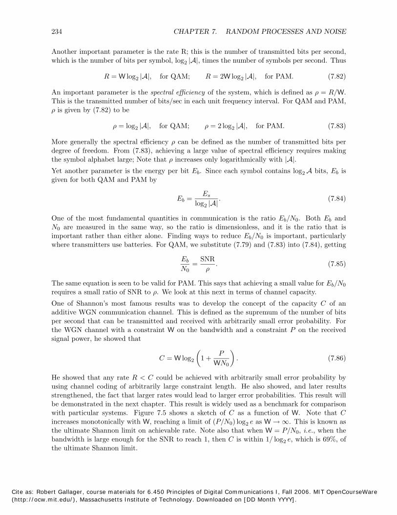
234 CHAPTER 7. RANDOM PROCESSES AND NOISE
Another important parameter is the rate R; this is the number of transmitted bits per second, which is the number of bits per symbol, log2 |A|, times the number of symbols per second. Thus
R = W log2 |A|, for QAM; R = 2W log2 |A|, for PAM. (7.82)
An important parameter is the spectral efficiency of the system, which is defined as ρ = R/W. This is the transmitted number of bits/sec in each unit frequency interval. For QAM and PAM, ρ is given by (7.82) to be
ρ = log2 |A|, for QAM; ρ = 2 log2 |A|, for PAM. (7.83)
More generally the spectral efficiency ρ can be defined as the number of transmitted bits per degree of freedom. From (7.83), achieving a large value of spectral efficiency requires making the symbol alphabet large; Note that ρ increases only logarithmically with |A|. Yet another parameter is the energy per bit Eb. Since each symbol contains log2 A bits, Eb is given for both QAM and PAM by
Eb = Es
. (7.84)log2 |A|
One of the most fundamental quantities in communication is the ratio Eb/N0. Both Eb and N0 are measured in the same way, so the ratio is dimensionless, and it is the ratio that is important rather than either alone. Finding ways to reduce Eb/N0 is important, particularly where transmitters use batteries. For QAM, we substitute (7.79) and (7.83) into (7.84), getting
Eb SNR = . (7.85)
N0 ρ
The same equation is seen to be valid for PAM. This says that achieving a small value for Eb/N0
requires a small ratio of SNR to ρ. We look at this next in terms of channel capacity.
One of Shannon’s most famous results was to develop the concept of the capacity C of an additive WGN communication channel. This is defined as the supremum of the number of bits per second that can be transmitted and received with arbitrarily small error probability. For the WGN channel with a constraint W on the bandwidth and a constraint P on the received signal power, he showed that
P C = W log2 1 + . (7.86)
WN0
He showed that any rate R < C could be achieved with arbitrarily small error probability by using channel coding of arbitrarily large constraint length. He also showed, and later results strengthened, the fact that larger rates would lead to larger error probabilities. This result will be demonstrated in the next chapter. This result is widely used as a benchmark for comparison with particular systems. Figure 7.5 shows a sketch of C as a function of W. Note that C increases monotonically with W, reaching a limit of (P/N0) log2 e as W → ∞. This is known as the ultimate Shannon limit on achievable rate. Note also that when W = P/N0, i.e., when the bandwidth is large enough for the SNR to reach 1, then C is within 1/ log2 e, which is 69%, of the ultimate Shannon limit.
Cite as: Robert Gallager, course materials for 6.450 Principles of Digital Communications I, Fall 2006. MIT OpenCourseWare (http://ocw.mit.edu/), Massachusetts Institute of Technology. Downloaded on [DD Month YYYY].
7.10. SUMMARY OF RANDOM PROCESSES 235
(P/N0) log2 e
P/N0
P/N0
W Figure 7.5: Capacity as a function of bandwidth W for fixed P/N0.
For any achievable rate, R, i.e., any rate at which the error probability can be made arbitrarily small by coding and other clever strategems, the theorem above says that R < C. If we rewrite (7.86), substituting SNR for P/(WN0) and substituting ρ for R/W, we get
ρ < log2(1 + SNR). (7.87)
If we substitute this into (7.85), we get
Eb SNR > .
N0 log2(1 + SNR)
This is a monotonic increasing function of the single variable SNR, which in turn is decreasing in W. Thus (Eb/N0)min is monotonic decreasing in W. As W → ∞ it reaches the limit ln 2 = 0.693, i.e., -1.59 dB. As W decreases, it grows, reaching 0 dB at SNR =1, and increasing without bound for yet smaller W. The limiting spectral efficiency, however, is C/W. This is also monotonic decreasing in W, going to 0 as W → ∞. In other words, there is a trade-off between Eb/N0
(which we would like to be small) and spectral efficiency (which we would like to be large). This is further discussed in the next chapter.
7.10 Summary of Random Processes
The additive noise in physical communication systems is usually best modeled as a random process, i.e., a collection of random variables, one at each real-valued instant of time. A random process can be specified by its joint probability distribution over all finite sets of epochs, but additive noise is most often modeled by the assumption that the random variables are all zero-mean Gaussian and their joint distribution is jointly Gaussian.
These assumptions were motivated partly by the central limit theorem, partly by the simplicity of working with Gaussian processes, partly by custom, and partly by various extremal properties. We found that jointly Gaussian means a great deal more than individually Gaussian, and that the resulting joint densities are determined by the covariance matrix. These densities have ellipsoidal equiprobability contours whose axes are the eigenfunctions of the covariance matrix.
A sample function, say Z(t, ω) of a random process Z(t) can be viewed as a waveform and interpreted as an L2 vector. For any fixed L2 function g(t), the inner product 〈g(t), Z(t, ω)〉maps ω into a real number and thus can be viewed over Ω as a random variable. This rv is called a linear function of Z(t) and is denoted by g(t)Z(t) dt.
Cite as: Robert Gallager, course materials for 6.450 Principles of Digital Communications I, Fall 2006. MIT OpenCourseWare (http://ocw.mit.edu/), Massachusetts Institute of Technology. Downloaded on [DD Month YYYY].

236 CHAPTER 7. RANDOM PROCESSES AND NOISE
These linear functionals arise when expanding a random process into an orthonormal expansion and also at each epoch when a random process is passed through a linear filter. For simplicity these linear functionals and the underlying random processes are not viewed in a measure theoretic form, although the L2 development in Chapter 4 provides some insight about the mathematical subtleties involved.
Noise processes are usually viewed as being stationary, which effectively means that their statistics do not change in time. This generates two problems - first that the sample functions have infinite energy and second that there is no clear way to see whether results are highly sensitive to time-regions far outside the region of interest. Both of these problems are treated by defining effective stationarity (or effective wide-sense stationarity) in terms of the behavior of the process over a finite interval. This analysis shows, for example, that Gaussian linear functionals depend only on effective stationarity over the region of interest. From a practical standpoint, this means that the simple results arising from the assumption of stationarity can be used without concern for the process statistics outside the time-range of interest.
The spectral density of a stationary process can also be used without concern for the process outside the time-range of interest. If a process is effectively WSS, it has a single variable covariance function corresponding to the interval of interest, and this has a Fourier transform which operates as the spectral density over the region of interest. How these results change as the region of interest approaches ∞ is explained in Appendix 7A.3.
7A Appendix: Supplementary topics
7A.1 Properties of covariance matrices
This appendix summarizes some properties of covariance matrices that are often useful but not absolutely critical to our treatment of random processes. Rather than repeat everything twice, we combine the treatment for real and complex rv together. On a first reading, however, one might assume everything to be real. Most of the results are the same in each case, although the complex-conjugate signs can be removed in the real case. It is important to realize that the properties developed here apply to nonGaussian as well as Gaussian rv’s. All rv’s and rv’s here are assumed to be zero-mean.
A square matrix K is a covariance matrix if a (real or complex) rv Z exists such that K = E[ZZ T∗]. The complex conjugate of the transpose, Z T∗, is called the Hermitian transpose and denoted by Z †. If Z is real, of course, Z † = Z T . Similarly, for a matrix K, the Hermitian conjugate, denoted K†, is KT∗. A matrix is Hermitian if K = K†. Thus a real Hermitian matrix (a Hermitian matrix containing all real terms) is a symmetric matrix.
An n by n square matrix K with real or complex terms is nonnegative definite if it is Hermitian and if, for all b ∈ Cn , b†Kb is real and nonnegative. It is positive definite if, in addition, b†Kb > 0 for b = 0. We now list some of the important relationships between nonnegative definite, positive definite, and covariance matrices and state some other useful properties of covariance matrices.
1. Every covariance matrix K is nonnegative definite. To see this, let Z be a rv such that K = E[ZZ †]. K is Hermitian since E[ZkZ
∗ ] = E[Z∗ Zk] for all k,m. For any b ∈ Cn, let m m
X = b†Z . Then 0 ≤ E[|X|2] = E (b†Z )(b†Z )∗ = E b†ZZ †b = b†Kb.
Cite as: Robert Gallager, course materials for 6.450 Principles of Digital Communications I, Fall 2006. MIT OpenCourseWare (http://ocw.mit.edu/), Massachusetts Institute of Technology. Downloaded on [DD Month YYYY].
7A. APPENDIX: SUPPLEMENTARY TOPICS 237
2. For any complex n by n matrix A, the matrix K = AA† is a covariance matrix. In fact, let Z have n independent unit-variance elements so that KZ is the identity matrix In. Then Y = AZ has the covariance matrix KY = E[(AZ )(AZ )†] = E[AZZ †A†] = AA†. Note that if A is real and Z is real, then Y is real and, of course, KY is real. It is also possible for A to be real and Z complex, and in this case KY is still real but Y is complex.
3. A covariance matrix K is positive definite if and only if K is nonsingular. To see this, let K = E[ZZ †] and note that if b†Kb = 0 for some b = 0, then X = b†Z has zero variance, and therefore is zero with probability 1. Thus E[XZ †] = 0, so b†E[ZZ †] = 0. Since b = 0 and b†K = 0, K must be singular. Conversely, if K is singular, there is some b such that Kb = 0, so b†Kb is also 0.
4. A complex number λ is an eigenvalue of a square matrix K if Kq = λq for some nonzero vector q ; the corresponding q is an eigenvector of K. The following results about the eigenvalues and eigenvectors of positive (nonnegative) definite matrices K are standard linear algebra results (see for example, Strang, section 5.5): All eigenvalues of K are positive (nonnegative). If K is real, the eigenvectors can be taken to be real. Eigenvectors of different eigenvalues are orthogonal, and the eigenvectors of any one eigenvalue form a subspace whose dimension is called the multiplicity of that eigenvalue. If K is n by n, then n orthonormal eigenvectors, q1, . . . , qn can be chosen. The corresponding list of eigenvalues, λ1, . . . , λn need not be distinct; specifically, the number of repetitions of each eigenvalue equals the multiplicity of that eigenvalue. Finally det(K) = k
n =1 λk.
5. If K is nonnegative definite, let Q be the matrix with the orthonormal columns, q1, . . . , qn
defined above. Then Q satisfies KQ = QΛ where Λ = diag(λ1, . . . , λn). This is simply the vector version of the eigenvector/eigenvalue relationship above. Since q †
kqm = δnm, Q also satisfies Q†Q = In. We then also have Q−1 = Q† and thus QQ† = In; this says that the rows of Q are also orthonormal. Finally, by post-multiplying KQ = QΛ by Q†, we see that K = QΛQ†. The matrix Q is called unitary if complex, and orthogonal if real.
6. If K is positive definite, then Kb = 0 for b = 0. Thus K can have no zero eigenvalues and Λ is nonsingular. It follows that K can be inverted as K−1 = QΛ−1Q†. For any n-vector b,
b†K−1b = λ−k
1|〈b, qk〉|2 . k
To see this, note that b†K−1b = b†QΛ−1Q†b. Letting v = Q†b and using the fact that the rows of QT are the orthonormal vectors qk, we see that 〈b, qk〉 is the kth component of v . We then have v †Λ−1v = k λ
−k
1|vk|2, which is equivalent to the desired result. Note that 〈b, qk〉 is the projection of b in the direction of qk.
7. det K = nk=1 λk where λ1, . . . , λn are the eigenvalues of K repeated according to their
multiplicity. Thus if K is positive definite, det K > 0 and if K is nonnegative definite, det K ≥ 0.
8. If K is a positive definite (semi-definite) matrix, then there is a unique positive definite (semi-definite) square root matrix R satisfying R2 = K. In particular, R is given by
R = QΛ1/2Q† whereΛ1/2 = diag λ1, λ2, . . . , λn . (7.88)
9. If K is nonnegative definite, then K is a covariance matrix. In particular, K is the covariance matrix of Y = RV where R is the square root matrix in (7.88) and KV = Im
Cite as: Robert Gallager, course materials for 6.450 Principles of Digital Communications I, Fall 2006. MIT OpenCourseWare (http://ocw.mit.edu/), Massachusetts Institute of Technology. Downloaded on [DD Month YYYY].
238 CHAPTER 7. RANDOM PROCESSES AND NOISE
This shows that zero-mean jointly-Gaussian rv’s exist with any desired covariance matrix; the definition of jointly Gaussian here as a linear combination of normal rv’s does not limit the possible set of covariance matrices.
For any given covariance matrix K, there are usually many choices for A satisfying K = AAT . The square root matrix R above is simply a convenient choice. Some of the results in this section are summarized in the following theorem:
Theorem 7A.1. An n by n matrix K is a covariance matrix if and only if it is nonnegative definite. Also it is a covariance matrix if and only if K = AA† for an n by n matrix A. One choice for A is the square root matrix R in (7.88).
7A.2 The Fourier series expansion of a truncated random process
Consider a (real zero-mean) random process that is effectively WSS over some interval [−T0 T0 ]2 , 2
where T0 is viewed intuitively as being very large. Let Z(t); |t| ≤ T2 0 be this process trun
cated to the interval [−T0 T0 ]. The objective of this and the next appendix is to view this 2 , 2 truncated process in the frequency domain and discover its relation to the spectral density of an untruncated WSS process. A second objective is to interpret the statistical independence between different frequencies for stationary Gaussian processes in terms of a truncated process.
Initially assume that Z(t); |t| ≤ T2 0 is arbitrary; the effective WSS assumption will be added
later. Assume the sample functions of the truncated process are L2 real functions with probability 1. Each L2 sample function, say Z(t, ω); |t| ≤ T2
0 can then be expanded in a Fourier series,
Z(t, ω) = ∞
Zk(ω)e 2πikt/T0 , |t| ≤ T
2 0 . (7.89)
m=−∞
The orthogonal functions here are complex and the coefficients Zk(ω) can be similarly complex.Since the sample functions Z(t, ω); 2 are real, Zk(ω) = Z∗ (ω) for each k. This also|t| ≤ T0
−k
implies that Z0(ω) is real. The inverse Fourier series is given by T0 2
Zk(ω) = 1
Z(t, ω)e−2πikt/T0 dt. (7.90)T0 T0
2−
For each sample point ω, Zk(ω) is a complex number, so Zk is a complex random variable, i.e., (Zk) and (Zk) are each rv’s. Also, (Zk) = (Z−k) and (Zk) = −(Z−k) for each k. It follows that the truncated process Z(t); |t| ≤ T
2 0 defined by
Z(t) = ∞
Zke 2πikt/T0 , − T
2 0 ≤ t ≤
T
2 0 . (7.91)
k=−∞
is a (real) random process and the complex random variables Zk are complex linear functionals of Z(t) given by T0
Zk =1 2
Z(t)e−2πikt/T0 dt. (7.92)T0 T0
2−
Cite as: Robert Gallager, course materials for 6.450 Principles of Digital Communications I, Fall 2006. MIT OpenCourseWare (http://ocw.mit.edu/), Massachusetts Institute of Technology. Downloaded on [DD Month YYYY].
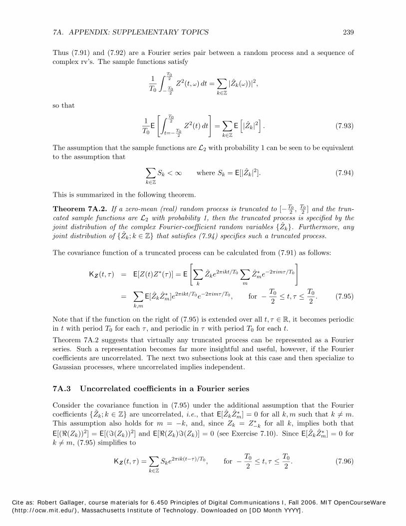
7A. APPENDIX: SUPPLEMENTARY TOPICS 239
Thus (7.91) and (7.92) are a Fourier series pair between a random process and a sequence of complex rv’s. The sample functions satisfy
1 T
20
Z2(t, ω) dt =
Zk(ω)) 2 ,T0 − T0
k∈Z
| |2
so that
1 T
20
T0
E T0
Z2(t) dt = E |Zk|2 . (7.93) t=−
2 k∈Z
The assumption that the sample functions are L2 with probability 1 can be seen to be equivalent to the assumption that
Sk < ∞ where Sk = E[|Zk|2]. (7.94) k∈Z
This is summarized in the following theorem.
Theorem 7A.2. If a zero-mean (real) random process is truncated to [−T2 0 , T0 ] and the trun2
cated sample functions are L2 with probability 1, then the truncated process is specified by the joint distribution of the complex Fourier-coefficient random variables Zk. Furthermore, any joint distribution of Zk; k ∈ Z that satisfies (7.94) specifies such a truncated process.
The covariance function of a truncated process can be calculated from (7.91) as follows:
KZ (t, τ) = E[Z(t)Z∗(τ)] = E Zke 2πikt/T0 Z∗ e−2πimτ/T0 m
k m
=
E[ZkZ∗ ]e 2πikt/T0e−2πimτ/T0 , for −
T
2 0 ≤ t, τ ≤
T0 . (7.95)m 2
k,m
Note that if the function on the right of (7.95) is extended over all t, τ ∈ R, it becomes periodic in t with period T0 for each τ , and periodic in τ with period T0 for each t.
Theorem 7A.2 suggests that virtually any truncated process can be represented as a Fourier series. Such a representation becomes far more insightful and useful, however, if the Fourier coefficients are uncorrelated. The next two subsections look at this case and then specialize to Gaussian processes, where uncorrelated implies independent.
7A.3 Uncorrelated coefficients in a Fourier series
Consider the covariance function in (7.95) under the additional assumption that the Fourier coefficients Zk; k ∈ Z are uncorrelated, i.e., that E[ZkZ
∗ ] = 0 for all k,m such that k = m.m
This assumption also holds for m = −k, and, since Zk = Z∗ for all k, implies both that −k
E[((Zk))2] = E[((Zk))2] and E[(Zk)(Zk)] = 0 (see Exercise 7.10). Since E[ZkZ∗ ] = 0 for m
k = m, (7.95) simplifies to
KZ (t, τ) = Ske 2πik(t−τ)/T0 , for − T
2 0 ≤ t, τ ≤
T0 . (7.96)
2 k∈Z
Cite as: Robert Gallager, course materials for 6.450 Principles of Digital Communications I, Fall 2006. MIT OpenCourseWare (http://ocw.mit.edu/), Massachusetts Institute of Technology. Downloaded on [DD Month YYYY].
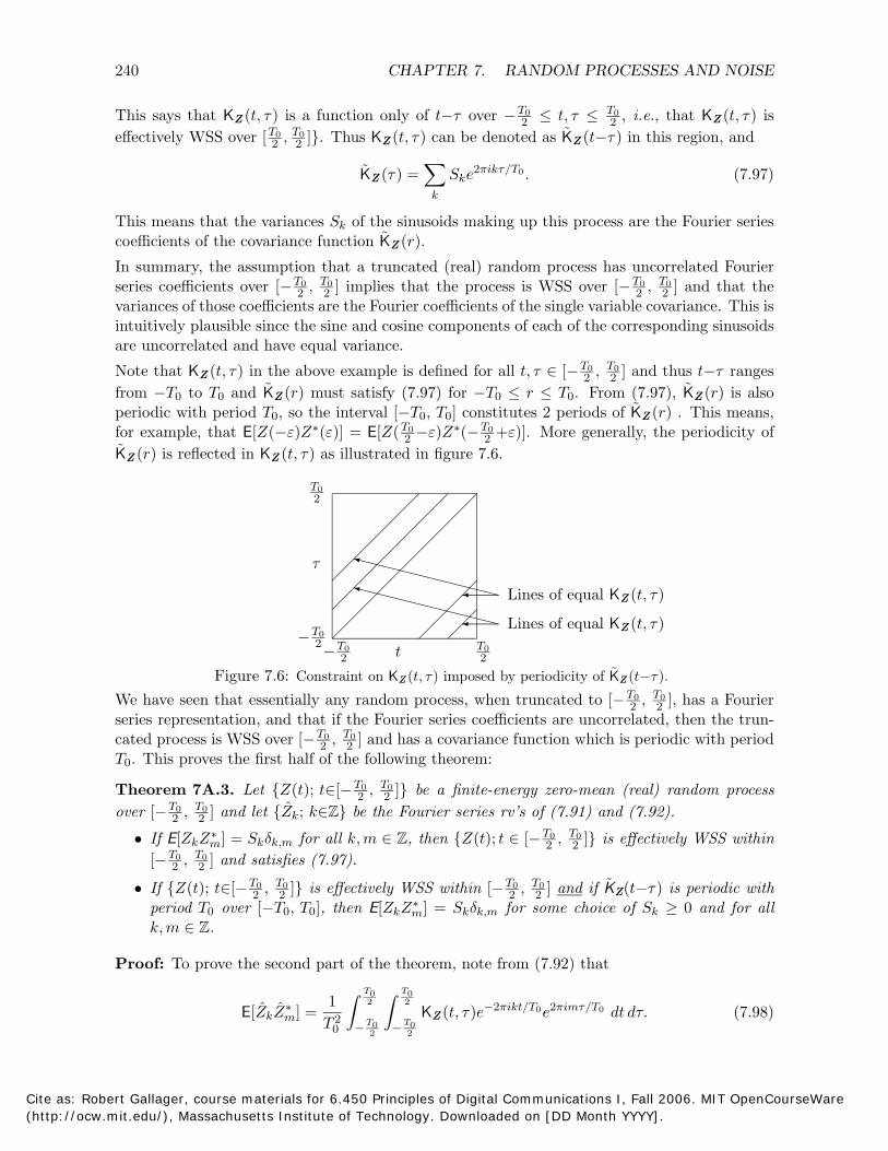
240 CHAPTER 7. RANDOM PROCESSES AND NOISE
This says that KZ (t, τ) is a function only of t−τ effectively WSS over [T
2 , T00
over −T2 0 ≤ t, τ ≤ T
2 0 , i.e., that KZ (t, τ) is
]. Thus KZ (t, τ ) can be denoted as KZ (t−τ) in this region, and2
KZ (τ ) = Ske 2πikτ/T0 . (7.97) k
This means that the variances Sk of the sinusoids making up this process are the Fourier series coefficients of the covariance function KZ (r).
In summary, the assumption that a truncated (real) random process has uncorrelated Fourier 00T T T T
2 , ] implies that the process is WSS over [− 2 , variances of those coefficients are the Fourier coefficients of the single variable covariance. This is
00series coefficients over [− ] and that the2 2
intuitively plausible since the sine and cosine components of each of the corresponding sinusoids are uncorrelated and have equal variance.
00Note that KZ (t, τ ) in the above example is defined for all t, τ ∈ [−T2 ,
T
from −T0 to T0 and KZ (r) must satisfy (7.97) for −T0 ≤ r ≤ T0.
0
periodic with period T0, so the interval [−T0, T0] constitutes 2 periods of ˜
2 −ε)Z∗(−T0
] and thus t−τ ranges From (7.97), KZ (r) is also
2
KZ (r) . This means, for example, that E[Z(−ε)Z∗(ε)] = E[Z(T
KZ (r) is reflected in KZ (t, τ) as illustrated in figure 7.6.+ε)]. More generally, the periodicity of2
T2
τ
0
0
Lines of equal KZ (t, τ)
Lines of equal KZ (t, τ)T−2 0T
2 t 0T2−
00
Figure 7.6: Constraint on KZ (t, τ) imposed by periodicity of KZ (t−τ). T TWe have seen that essentially any random process, when truncated to [− 2 ,
series representation, and that if the Fourier series coefficients are uncorrelated, then the trun], has a Fourier2
00cated process is WSS over [−T2 ,
T
T0. This proves the first half of the following theorem:] and has a covariance function which is periodic with period2
00
00T T2 , ] be a finite-energy zero-mean (real) random process
Zk; k∈Z be the Fourier series rv’s of (7.91) and (7.92). T T
00
Theorem 7A.3. Let Z(t); t∈[−T T2 , ] and let
2 ˆover [− 2
00
If E[ZkZ∗ ] = Skδk,m for all k,m ∈ Z, then Z(t); t ∈ [−• m 2 , 2
T T
] is effectively WSS within[− ] and satisfies (7.97).2 ,
If Z(t); t∈[−2
] and if ˜0000T T T T2 , 2 ,
period T0 over [−T0, T0], then E[ZkZ∗ ] = Skδk,m for some choice of Skm
k,m ∈ Z.
Proof: To prove the second part of the theorem, note from (7.92) that
] is effectively WSS within [− KZ(t−τ ) is periodic with ≥ 0 and for all
2 2•
0 2
0 2
T T
E[ZkZ∗ ] =
1 m KZ (t, τ )e−2πikt/T0 2πimτ/T0e dt dτ. (7.98)
T 2 0 0 2
T − 0 2
T−
Cite as: Robert Gallager, course materials for 6.450 Principles of Digital Communications I, Fall 2006. MIT OpenCourseWare (http://ocw.mit.edu/), Massachusetts Institute of Technology. Downloaded on [DD Month YYYY].
7A. APPENDIX: SUPPLEMENTARY TOPICS 241
T0 T0By assumption, KZ (t, τ) = KZ (t−τ ) for t, τ ∈ [− 2 , 2 ] and KZ (t − τ) is periodic with period T0. Substituting s = t−τ for t as a variable of integration, (7.98) becomes T0
T0
E[ZkZ∗ ] =
1 2 2 −τ
KZ (s)e−2πiks/T0 ds e−2πikτ/T0e 2πimτ/T0 dτ. (7.99)m T 2 T0 T00 − 2
− 2 −τ
The integration over s does not depend on τ because the interval of integration is one period and KZ is periodic. Thus this integral is only a function of k, which we denote by T0Sk. Thus T0
E[ZkZ∗ ] =
1 2
Ske−2πi(k−m)τ/T0 dτ =
Sk for m = k (7.100)m T0 T0 0 otherwise
2−
This shows that the Zk are uncorrelated, completing the proof.
The next issue is to find the relationship between these processes and processes that are WSS over all time. This can be done most cleanly for the case of Gaussian processes. Consider a WSS (and therefore stationary) zero-mean Gaussian random process25 Z ′(t); t ∈ R with covariance function KZ ′ (τ ) and assume a limited region of nonzero covariance
i.e.,
KZ ′ (τ) = 0 for |τ | >T
2 1 .
Let SZ′ (f) ≥ 0 be the spectral density of Z ′ and let T0 satisfy T0 > T1. The Fourier series coefficients of KZ ′ (τ) over the interval [−T
2 0 , T0 ] are then given by Sk = SZ′ (k/T0) . Suppose this process 2 T0
is approximated over the interval [−T2 0 , T
2 0 ] by a truncated Gaussian process Z(t); t∈[−T
2 0 , T
2 0 ]
composed of independent Fourier coefficients Zk, i.e.
Z(t) =
Zke 2πikt/T0 , − T
2 0 ≤ t ≤
T
2 0 ,
k
where
E[ZkZ∗ for all k,m ∈ Z.m] = Skδk,m
2πikt/T0By Theorem 7A.3, the covariance function of Z(t) is KZ (τ) =
k Ske . This is periodic with period T0 and for T
2 0 , KZ (τ) = KZ ′ (τ). The original process Z (t) and the approx|τ | ≤
T0 T0
′
imation Z(t) thus have the same covariance for |τ | ≤ 2 . For |τ | > 2 , KZ ′ (τ ) = 0 whereas KZ (τ) is periodic over all τ . Also, of course, Z ′ is stationary, whereas Z is effectively stationary within its domain [−T
2 0 , T0 ]. The difference between Z and Z ′ becomes more clear in terms of 2
the two-variable covariance function, illustrated in Figure 7.7.
It is evident from the figure that if Z ′ is modeled as a Fourier series over [−T2 0 , T0 ] using2
independent complex circularly symmetric Gaussian coefficients, then KZ′ (t, τ) = KZ (t, τ) for |t|, |τ | ≤ T0−T1 . Since zero-mean Gaussian processes are completely specified by their covariance 2 functions, this means that Z ′ and Z are statistically identical over this interval.
In summary, a stationary Gaussian process Z ′ can not be perfectly modeled over an interval[−T
2 0 , T
2 0 ] by using a Fourier series over that interval. The anomalous behavior is avoided,
25Equivalently, one can assume that Z′ is effectively WSS over some interval much larger than the intervals of interest here.
Cite as: Robert Gallager, course materials for 6.450 Principles of Digital Communications I, Fall 2006. MIT OpenCourseWare (http://ocw.mit.edu/), Massachusetts Institute of Technology. Downloaded on [DD Month YYYY].
|
242 CHAPTER 7. RANDOM PROCESSES AND NOISE
T0 T0 2 2
τ τ
T1
T0 T0 2 2−
T0 t T0
−T0 t T0
2 2 2 2−(a)
−(b)
Figure 7.7: Part (a) illustrates KZ (t, τ) over the region −T0 ≤ t, τ ≤ T0 for a stationary2 2
process Z ′ satisfying KZ (τ ) = 0 for |τ | > T1/2. Part (b) illustrates the approximating process Z comprised of independent sinusoids, spaced by 1/T0 and with uniformly distribuited phase. Note that the covariance functions are identical except for the anomalous behavior at the corners where t is close to T0/2 and τ is close to −T0/2 or vice versa.
however, by using a Fourier series over a larger interval, large enough to include the interval of interest plus the interval over which KZ ′ (τ) = 0. If this latter interval is unbounded, then theFourier series model can only be used as an approximation. The following theorem has been established.
Theorem 7A.4. Let Z ′(t) be a zero-mean stationary Gaussian random process with spectral density S(f) and covariance KZ′ (τ) = 0 for τ | ≥ T1/2. Then for T0 > T1, the truncated process Z(t) = Zke
2πikt/T0 for |t| ≤ T0 , where the Zk are independent and Zk ∼ CN (S(k/T0)) for allk 2 T0
k ∈ Z is statistically identical to Z ′(t) over [−T0−2
T1 , T0−2
T1 ].
The above theorem is primarily of conceptual use, rather than as a problem solving tool. It shows that, aside from the anomalous behavior discussed above, stationarity can be used over the region of interest without concern for how the process behaves outside far outside the interval of interest. Also, since T0 can be arbitrarily large, and thus the sinusoids arbitrarily closely spaced, we see that the relationship between stationarity of a Gaussian process and independence of frequency bands is quite robust and more than something valid only in a limiting sense.
7A.4 The Karhunen-Loeve expansion
There is another approach, called the Karhunen-Loeve expansion for representing a random process that is truncated to some interval [−T
2 0 , T
2 0 ] by an orthonormal expansion. The objec
tive is to choose a set of orthonormal functions such that the coefficients in the expansion are uncorrelated.
We start with the covariance function K(t, τ) defined for t, τ ∈ [−T2 0 , T
2 0 ]. The basic facts about
these time-limited covariance functions are virtually the same as the facts about covariance matrices in Appendix 7A.1. K(t, τ) is nonnegative definite in the sense that for all L2 functions g(t), T0 T0
2 2
g(t)KZ (t, τ)g(τ ) dt dτ ≥ 0 T0 T0 2 2
− −
KZ also has real valued orthonormal eigenvectors defined over [−T2 0 , T
2 0 ] and nonnegative eigen-
Cite as: Robert Gallager, course materials for 6.450 Principles of Digital Communications I, Fall 2006. MIT OpenCourseWare(http://ocw.mit.edu/), Massachusetts Institute of Technology. Downloaded on [DD Month YYYY].
7A. APPENDIX: SUPPLEMENTARY TOPICS 243
values. That is T0 2 T0 T0
KZ (t, τ)φm(τ ) dτ = λmφm(t); t ∈ − 2
, 2
where 〈φm, φk〉 = δm,k − T0
2
These eigenvectors span the L2 space of real functions over [−T T
as the orthonormal functions of Z(t) = Zmφm(t), it is easy to show that E[Zm
00 ]. By using these eigenvectors2 , 2 Zk] = λmδm,k. m
0In other words, given an arbitrary covariance function over the truncated interval [−T T
can find a particular set of orthonormal functions so that Z(t) = Zmφm(t) and E[Zm
0 2 ], we2 , Zk] =m
λmδm,k. This is called the Karhunen-Loeve expansion.
These equations for the eigenvectors and eigenvalues are well-known integral equations and can be calculated by computer. Unfortunately they do not provide a great deal of insight into the frequency domain.
Cite as: Robert Gallager, course materials for 6.450 Principles of Digital Communications I, Fall 2006. MIT OpenCourseWare (http://ocw.mit.edu/), Massachusetts Institute of Technology. Downloaded on [DD Month YYYY].
244 CHAPTER 7. RANDOM PROCESSES AND NOISE
7.E Exercises
7.1. (a) Let X, Y be iid rv’s, each with density f (x) = α exp(−x2/2). In part (b), we show X
that α must be 1/√
2π in order for fX (x) to integrate to 1, but in this part, we leave α undetermined. Let S = X2 + Y 2 . Find the probability density of S in terms of α. Hint: Sketch the contours of equal probability density in the X, Y plane. (b) Prove from part (a) that α must be 1/
√2π in order for S, and thus X and Y , to be
random variables. Show that E[X] = 0 and that E[X2] = 1. (c) Find the probability density of R =
√S. R is called a Rayleigh rv.
7.2. (a) Let X ∼ N (0, σ2 ) and Y ∼ N (0, σ2 ) be independent zero-mean Gaussian rv’s. By X Y convolving their densities, find the density of X+Y . Hint: In performing the integration for the convolution, you should do something called “completing the square” in the exponent. This involves multiplying and dividing by eαy2/2 for some α, and you can be guided in this by knowing what the answer is. This technique is invaluable in working with Gaussian rv’s. (b) The Fourier transform of a probability density fX (x) is fX (θ) =
fX (x)e−2πixθ dx =
E[e−2πiXθ]. By scaling the basic Gaussian transform in (4.48), show that for X ∼ N (0, σ2 ),X
(2πθ)2σ2
fX (θ) = exp − 2
X .
(b) Now find the density of X + Y by using Fourier transforms of the densities. (c) Using the same Fourier transform technique, find the density of V = k
n =1 αkWk where
W1, . . . , Wk are independent normal rv’s.
7.3. In this exercise you will construct two rv’s that are individually Gaussian but not jointly Gaussian. Consider the nonnegative random variable X with the density
fX (x) = 2
exp −x2
for x ≥ 0. π 2
Let U be binary, ±1, with pU (1) = pU (−1) = 1/2. (a) Find the probability density of Y1 = UX. Sketch the density of Y1 and find its mean and variance. (b) Describe two normalized Gaussian rv’s, say Y1 and Y2, such that the joint density of Y1, Y2 is zero in the second and fourth quadrants of the plane. It is nonzero in the first
2 2
and third quadrants where it has the density π 1 exp(−y1
2−y2 ). Hint: Use part (a) for Y1 and
think about how to construct Y2. (c) Find the covariance E[Y1Y2]. Hint: First find the mean of the rv X above. (d) Use a variation of the same idea to construct two normalized Gaussian rv’s V1, V2
whose probability is concentrated on the diagonal axes v1 = v2 and v1 = v2, i.e., for −which Pr(V1 = V2 and V1 = −V2) = 0.
7.4. Let W1 ∼ N (0, 1) and W2 ∼ N (0, 1) be independent normal rv’s. Let X = max(W1, W2) and Y = min(W1, W2). (a) Sketch the transformation from sample values of W1, W2 to sample values of X, Y . Which sample pairs w1, w2 of W1, W2 map into a given sample pair x, y of X, Y ?
Cite as: Robert Gallager, course materials for 6.450 Principles of Digital Communications I, Fall 2006. MIT OpenCourseWare (http://ocw.mit.edu/), Massachusetts Institute of Technology. Downloaded on [DD Month YYYY].
7.E. EXERCISES 245
(b) Find the probability density fXY (x, y) of X, Y . Explain your argument briefly but work from your sketch rather than equations. (c) Find fS(s) where S = X + Y . (d) Find fD(d) where D = X − Y . (e) Let U be a random variable taking the values ±1 with probability 1/2 each and let U be statistically independent of W1, W2. Are S and UD jointly Gaussian?
7.5. Let φ(t) be an L2 function of energy 1 and let h(t) be L2. Show that ∞φ(t)h(τ − t) dt
2 −∞
is an L2 function of τ with energy upper bounded by ‖h‖ . Hint: Consider the Fourier transform of φ(t) and h(t).
7.6. (a) Generalize the random process of (7.30) by assuming that the Zk are arbitrarily correlated. Show that every sample function is still L2. (b) For this same case, show that |KZ(t, τ)|2 dtdτ < ∞.
7.7. (a) Let Z1, Z2, . . . , be a sequence of independent Gaussian rv’s, Zk ∼ N (0, σk2) and let
φk(t) : R R be a sequence of orthonormal functions. Argue from fundamental def→ ninitions that for each t, Z(t) = k=1 Zkφk(t) is a Gaussian random variable. Find the variance of Z(t) as a function of t. (b) For any set of epochs, t1, . . . , t, let Z(tm) = k
n =1 Zkφk(tm) for 1 ≤ m ≤ . Explain
carefully from the basic definitions why Z(t1), . . . , Z(t) are jointly Gaussian and specify their covariance matrix. Explain why Z(t); t ∈ R is a Gaussian random process. (c) Now let n = ∞ above and assume that σk
2 < ∞. Also assume that the orthonormal k functions are bounded for all k and t in the sense that for some constant A, |φk(t)| ≤ A for all k and t. Consider the linear combination of rv’s
n
Z(t) = Zkφk(t) = lim Zkφk(t) k
n→∞ k=1
Let Z(n)(t) = n Zkφk(t). For any given t, find the variance of Z(j)(t) − Z(n)(t) for k=1
j > n. Show that for all j > n, this variance approaches 0 as n → ∞. Explain intuitively why this indicates that Z(t) is a Gaussian rv. Note: Z(t) is in fact a Gaussian rv, but proving this rigorously requires considerable background. Z(t) is a limit of a sequence of rv’s, and each rv is a function of a sample space - the issue here is the same as that of a sequence of functions going to a limit function, where we had to invoke the Riesz-Fischer theorem. (d) For the above Gaussian random process Z(t); t ∈ R, let z(t) be a sample function of Z(t) and find its energy, i.e., ‖z‖2 in terms of the sample values z1, z2, . . . of Z1, Z2, . . . . Find the expected energy in the process, E[‖Z(t); t ∈ R‖2]. (e) Find an upper bound on Pr‖Z(t); t ∈ R‖2 > α that goes to zero as α → ∞. Hint: You might find the Markov inequality useful. This says that for a nonnegative rv Y , PrY ≥ α ≤ E[Y ] . Explain why this shows that the sample functions of Z(t) are L2α with probability 1.
7.8. Consider a stochastic process Z(t); t ∈ R for which each sample function is a sequence of rectangular pulses as in the figure below.
Cite as: Robert Gallager, course materials for 6.450 Principles of Digital Communications I, Fall 2006. MIT OpenCourseWare (http://ocw.mit.edu/), Massachusetts Institute of Technology. Downloaded on [DD Month YYYY].

246 CHAPTER 7. RANDOM PROCESSES AND NOISE
z z2−1
z0 z1
Analytically, Z(t) = ∞ Zkrect(t − k) where . . . Z−1, Z0, Z1, . . . is a sequence of iid k=−∞normal variables, Zk ∼ N (0, 1).. (a) Is Z(t); t ∈ R a Gaussian random process? Explain why or why not carefully. (b) Find the covariance function of Z(t); t ∈ R. (c) Is Z(t); t ∈ R a stationary random process? Explain carefully. (d) Now suppose the stochastic process is modified by introducing a random time shift Φ which is uniformly distributed between 0 and 1. Thus, the new process, V (t); t ∈ R is defined by V (t) = ∞ Zkrect(t − k − Φ). Find the conditional distribution of V (0.5)k=−∞conditional on V (0) = v. (e) Is V (t); t ∈ R a Gaussian random process? Explain why or why not carefully. (f) Find the covariance function of V (t); t ∈ R. (g) Is V (t); t ∈ R a stationary random process? It is easier to explain this than to write a lot of equations.
7.9. Consider the Gaussian sinc process, V (t) = Vk sinc t−kT where . . . , V−1, V0, V1, . . . , k T is a sequence of iid rv’s, Vk ∼ N (0, σ2). (a) Find the probability density for the linear functional V (t)sinc(T
t ) dt. (b) Find the probability density for the linear functional V (t)sinc(αt ) dt for α > 1.T
(c) Consider a linear filter with impulse response h(t) = sinc(αt ) where α > 1. Let Y (t)T be the output of this filter when V (t) above is the input. Find the covariance function of the process Y (t). Explain why the process is Gaussian and why it is stationary.
(d) Find the probability density for the linear functional Y (τ) = V (t)sinc(α(tT−τ )) dt for
α ≥ 1 and arbitrary τ . (e) Find the spectral density of Y (t); t ∈ R. (f) Show that Y (t); t ∈ R can be represented as Y (t) = Yksinc t−kT and characterize k T the rv’s Yk; k ∈ Z. (g) Repeat parts (c), (d), and (e) for α < 1. (h) Show that Y (t) in the α < 1 case can be represented as a Gaussian sinc process (like V (t) but with an appropriately modified value of T ).
(i) Show that if any given process Z(t); t ∈ R is stationary, then so is the process Y (t); t ∈R where Y (t) = Z2(t) for all t ∈ R.
7.10. (Complex random variables)(a) Suppose the zero-mean complex random variables Xk
and X−k satisfy X∗ = Xk for all k. Show that if E[XkX∗ ] = 0 then E[((Xk))2] =
E[((Xk))2] and E[−k (Xk)(X−k)] = 0.
−k
(b) Use this to show that if E[XkX∗ ] = 0 then E[(Xk)(X )] = 0, E[(Xk)(X )] = 0, m m m
and E[(Xk)(Xm)] = 0 for all m not equal to either k or −k.
7.11. Explain why the integral in (7.58) must be real for g1(t) and g2(t) real, but the integrand g1(f)SZ (f)g2
∗(f) need not be real.
Cite as: Robert Gallager, course materials for 6.450 Principles of Digital Communications I, Fall 2006. MIT OpenCourseWare (http://ocw.mit.edu/), Massachusetts Institute of Technology. Downloaded on [DD Month YYYY].
7.E. EXERCISES 247
7.12. (Filtered white noise) Let Z(t) be a White Gaussian noise process of spectral density N0/2. T(a) Let Y = 0 Z(t) dt. Find the probability density of Y . (b) Let Y (t) be the result of passing Z(t) through an ideal baseband filter of bandwidth W whose gain is adjusted so that its impulse response has unit energy. Find the joint distribution of Y (0) and Y (4
1 W).
(c) Find the probability density of
∞V = e−tZ(t) dt.
0
7.13. (Power spectral density) (a) Let φk(t) be any set of real orthonormal L2 waveforms whose transforms are limited to a band B, and let W (t) be white Gaussian noise with respect to B with power spectral density SW (f) = N0/2 for f ∈ B. Let the orthonormal expansion of W (t) with respect to the set φk(t) be defined by
W (t) = Wkφk(t), k
where Wk = 〈W (t), φk(t)〉. Show that Wk is an iid Gaussian sequence, and give the probability distribution of each Wk. (b) Let the band B be B = [−1/2T, 1/2T ], and let φk(t) = (1/
√T )sinc( t−kT ), k ∈ Z.T
Interpret the result of part (a) in this case.
7.14. (Complex Gaussian vectors) (a) Give an example of a 2 dimensional complex rv Z = (Z1, Z2) where Zk ∼ CN (0, 1) for k = 1, 2 and where Z has the same joint probability distribution as eiφZ for all φ ∈ [0, 2π] but where Z is not jointly Gaussian and thus not circularly symmetric. Hint: Extend the idea in part (d) of Exercise 7.3. (b) Suppose a complex random variable Z = Zre + iZim has the properties that Zre and Zim are individually Gaussian and that Z has the same probability density as eiφZ for all φ ∈ [0, 2π]. Show that Z is complex circularly symmetric Gaussian.
Cite as: Robert Gallager, course materials for 6.450 Principles of Digital Communications I, Fall 2006. MIT OpenCourseWare (http://ocw.mit.edu/), Massachusetts Institute of Technology. Downloaded on [DD Month YYYY].


