Query processing and
optimizationoptimization
Reading (5th edition): Chapters 6.1-6.3, 15.1-15.3, 15.7-15.8.2
Jose M. Peña
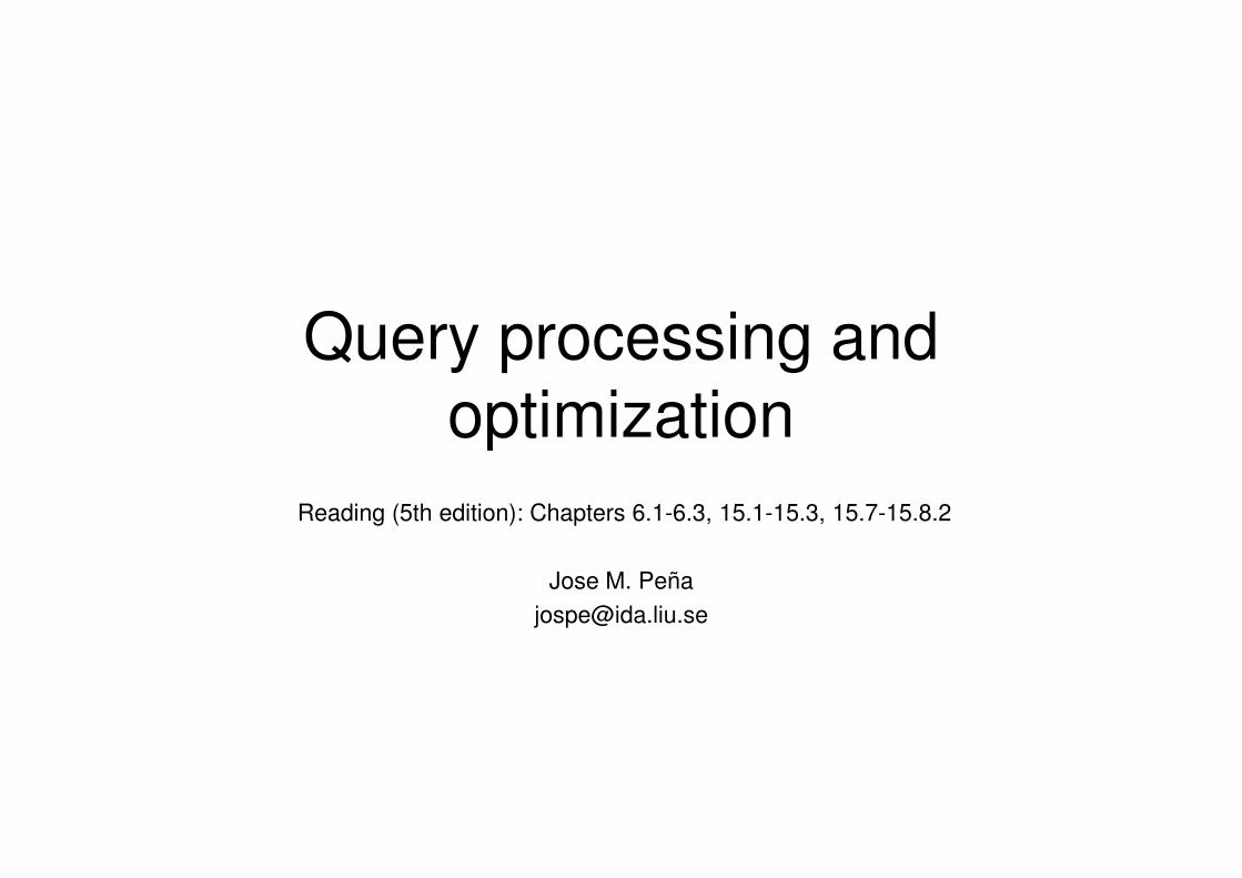
ER diagram
Relational model
MySQL
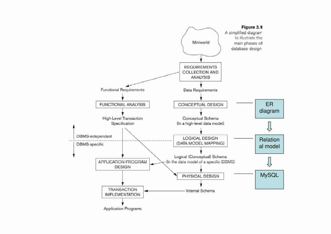
Relation schema
PNumber Name Address Telephone E-mail Age
Attributes
PNumber Name Address Telephone E-mail Age
yymmdd-xxxx
Textual string less than 30 chars
Textual string less than 30 chars
rrr - nn nn nn
aaaaannn
Positive integer
0<x<150
Domain = set of atomic values
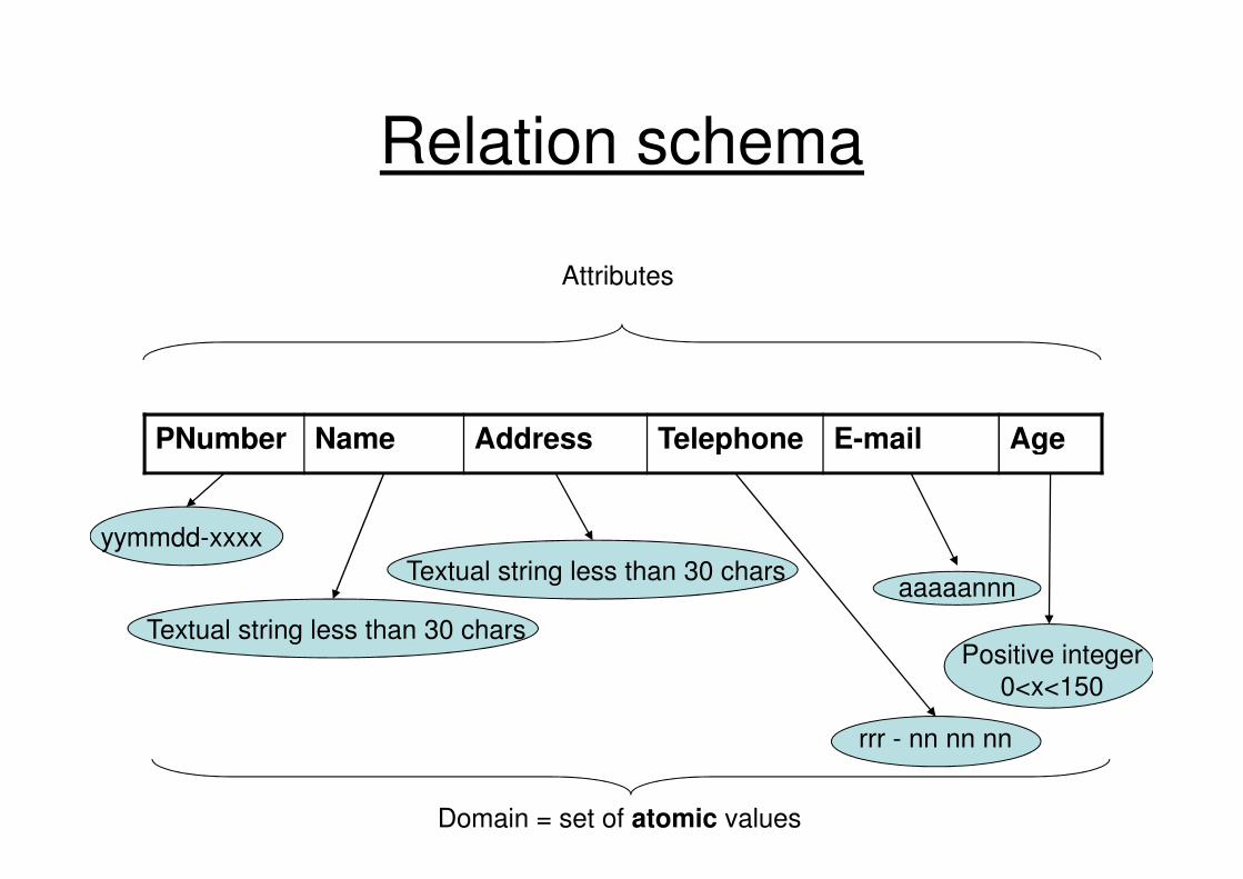
Relation (state)
PNumber Name Address Telephone E-mail Age
123456-7890 Anders
Andersson
Rydsvägen 1 013-11 22 33 andan111 25
112233-4455 Veronika Alsätersg 2 013-22 33 44 verpe222 27112233-4455 Veronika
Pettersson
Alsätersg 2 013-22 33 44 verpe222 27
Tuple = list of values in the corresponding domains, or NULL
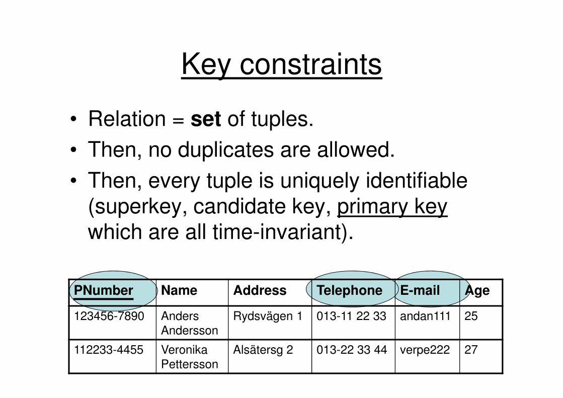
Key constraints
• Relation = set of tuples.
• Then, no duplicates are allowed.
• Then, every tuple is uniquely identifiable (superkey, candidate key, primary key(superkey, candidate key, primary keywhich are all time-invariant).
PNumber Name Address Telephone E-mail Age
123456-7890 Anders
Andersson
Rydsvägen 1 013-11 22 33 andan111 25
112233-4455 Veronika
Pettersson
Alsätersg 2 013-22 33 44 verpe222 27
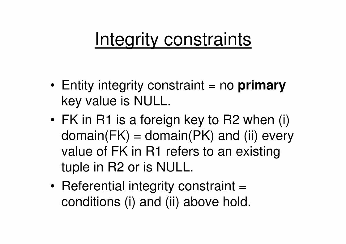
Integrity constraints
• Entity integrity constraint = no primarykey value is NULL.
• FK in R1 is a foreign key to R2 when (i) • FK in R1 is a foreign key to R2 when (i) domain(FK) = domain(PK) and (ii) every value of FK in R1 refers to an existing tuple in R2 or is NULL.
• Referential integrity constraint = conditions (i) and (ii) above hold.
Relational algebra
• Relational algebra = language for querying the relational model.
• Procedural language = how to carry out the query, as opposed to what to retrieve = query, as opposed to what to retrieve = declarative language, i.e. relational calculus.
• Basis for SQL.
• Basis for implementation and optimization of queries.
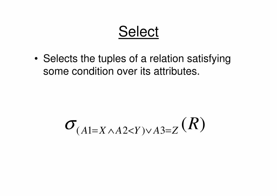
Select
• Selects the tuples of a relation satisfying some condition over its attributes.
)(3)21( RZAYAXA =∨<∧=σ

Example: select
PNum Name Address TelNr
112233-4455 Elin Rydsvägen 1 112233
223344-5566 Nisse Alsätersgatan 3 223344
334455-6677 Nisse Rydsvägen 3 334455
113322-1122 Pelle Rydsvägen 2 113322
STUDENT:
113322-1122 Pelle Rydsvägen 2 113322
552233-1144 Monika Rydsvägen 4 443322
442211-2222 Patrik Rydsvägen 6 111122
334433-1111 Camilla Alsätersgatan 1 665544
)('')'334455'''( STUDENTCamillaNameTelNrNisseName =∨=∧=
σ
PNum Name Address TelNr
334455-6677 Nisse Rydsvägen 3 334455
334433-1111 Camilla Alsätersgatan 1 665544
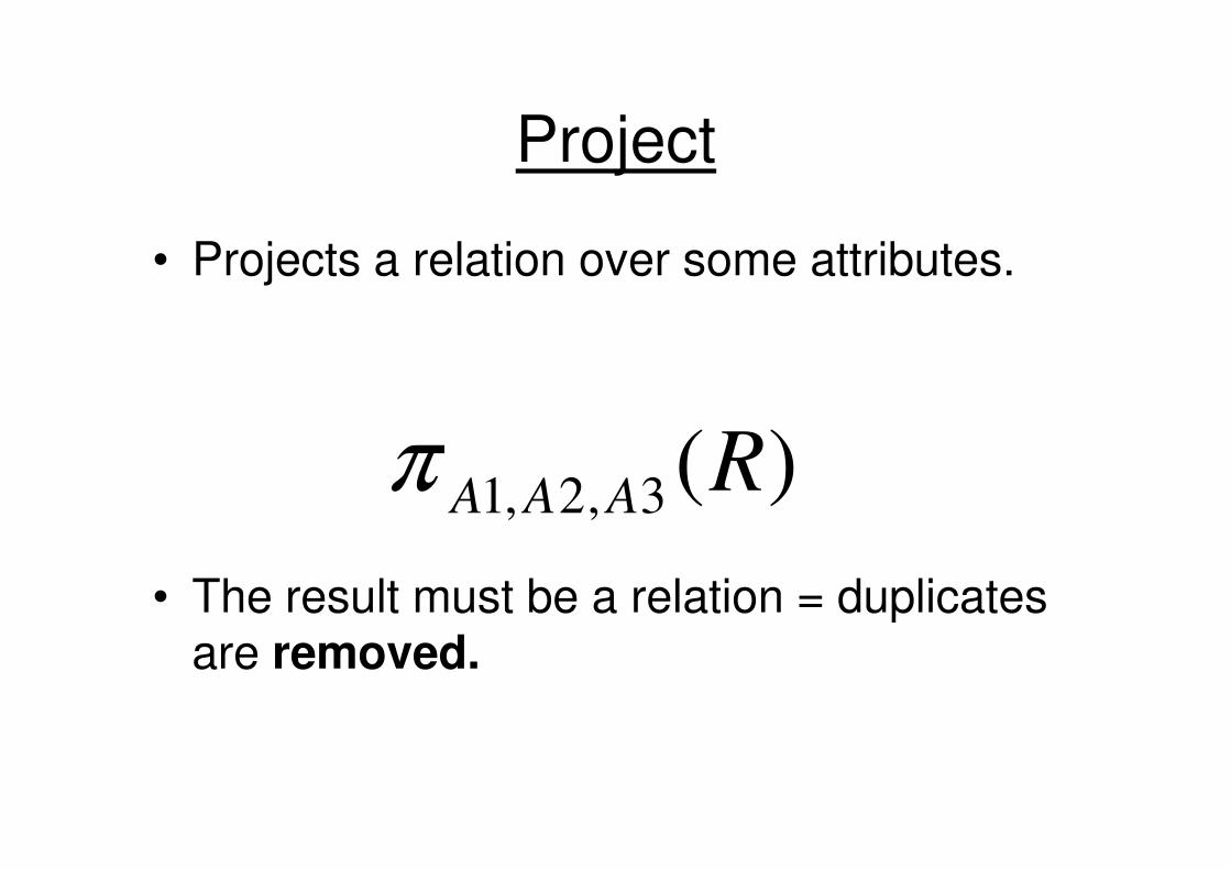
Project
• Projects a relation over some attributes.
)(Rπ
• The result must be a relation = duplicates are removed.
)(3,2,1 RAAA
π
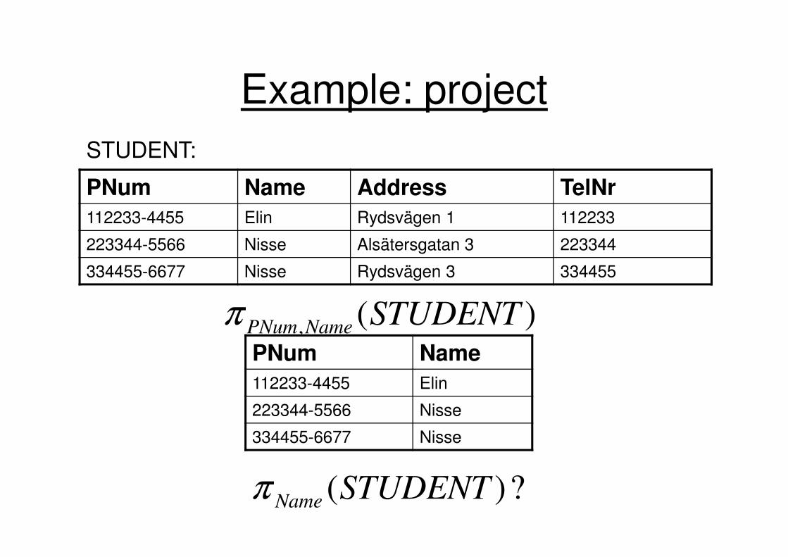
Example: project
PNum Name Address TelNr
112233-4455 Elin Rydsvägen 1 112233
223344-5566 Nisse Alsätersgatan 3 223344
334455-6677 Nisse Rydsvägen 3 334455
STUDENT:
)(, STUDENTNamePNum
π
334455-6677 Nisse Rydsvägen 3 334455
PNum Name
112233-4455 Elin
223344-5566 Nisse
334455-6677 Nisse
?)(STUDENTName
π
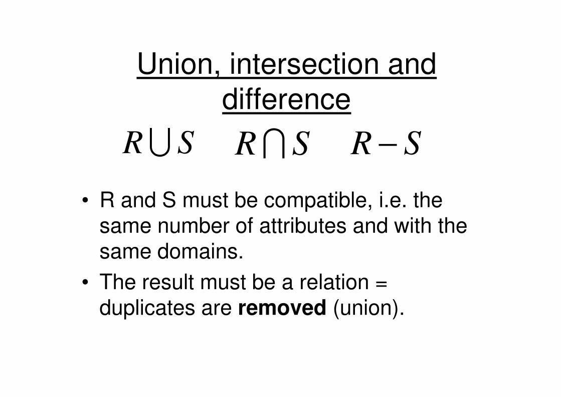
Union, intersection and
difference
• R and S must be compatible, i.e. the
SRISRU SR −
• R and S must be compatible, i.e. the same number of attributes and with the same domains.
• The result must be a relation = duplicates are removed (union).
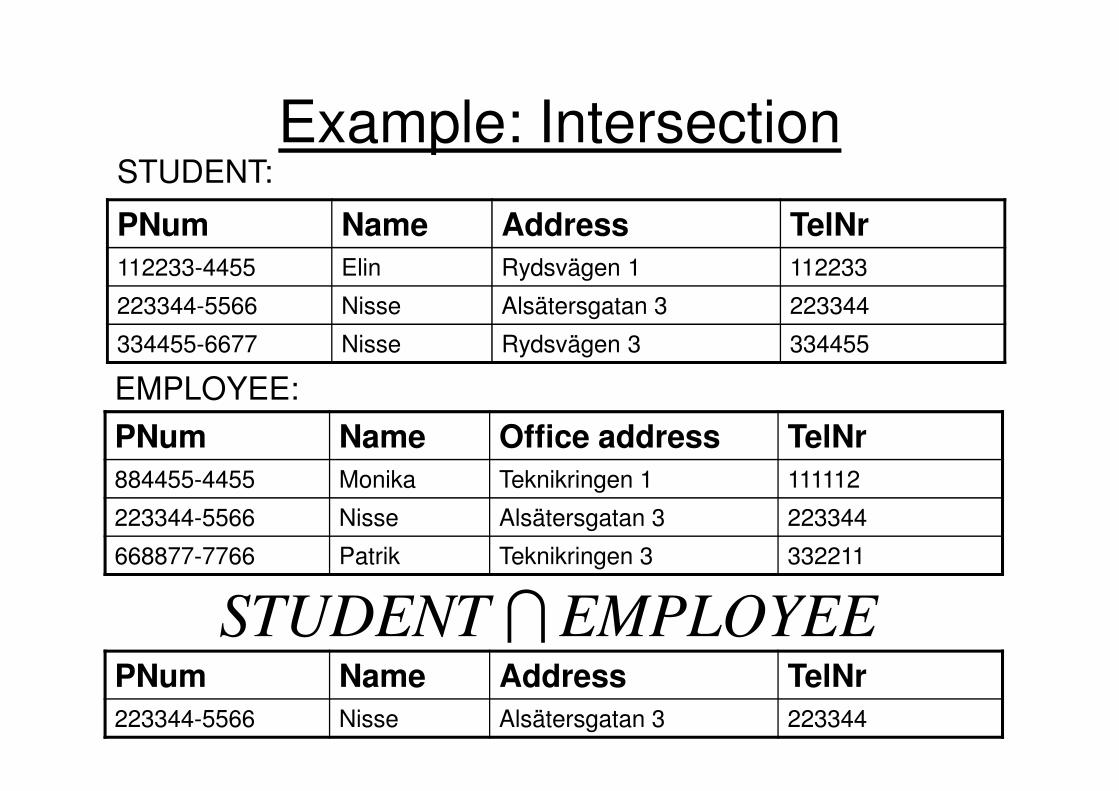
Example: Intersection
PNum Name Address TelNr
112233-4455 Elin Rydsvägen 1 112233
223344-5566 Nisse Alsätersgatan 3 223344
334455-6677 Nisse Rydsvägen 3 334455
STUDENT:
EMPLOYEE:
PNum Name Office address TelNr
884455-4455 Monika Teknikringen 1 111112
223344-5566 Nisse Alsätersgatan 3 223344
668877-7766 Patrik Teknikringen 3 332211
EMPLOYEE:
EMPLOYEESTUDENT IPNum Name Address TelNr
223344-5566 Nisse Alsätersgatan 3 223344
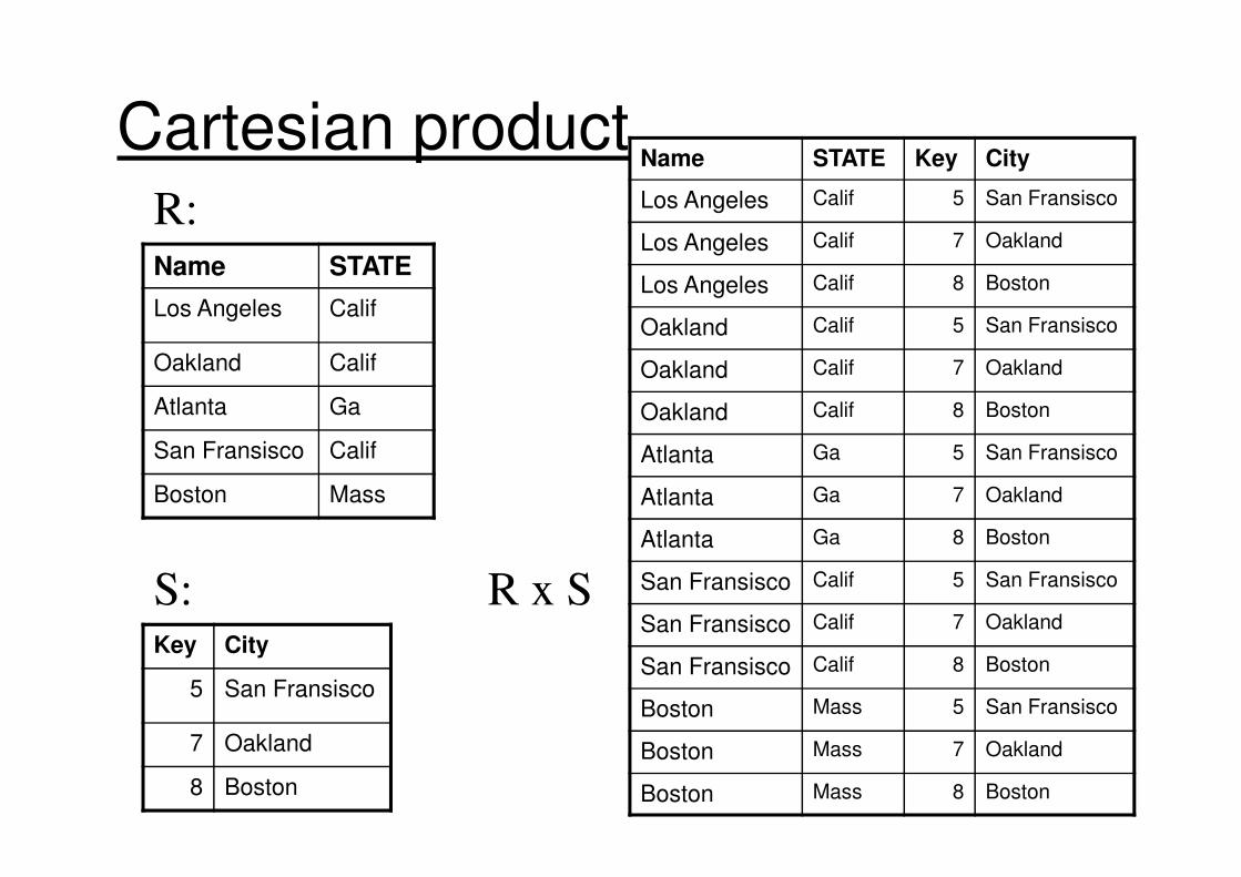
Cartesian product
Name STATE
Los Angeles Calif
Oakland Calif
Atlanta Ga
San Fransisco Calif
Name STATE Key City
Los Angeles Calif 5 San Fransisco
Los Angeles Calif 7 Oakland
Los Angeles Calif 8 Boston
Oakland Calif 5 San Fransisco
Oakland Calif 7 Oakland
Oakland Calif 8 Boston
R:
San Fransisco Calif
Boston Mass
Key City
5 San Fransisco
7 Oakland
8 Boston
Atlanta Ga 5 San Fransisco
Atlanta Ga 7 Oakland
Atlanta Ga 8 Boston
San Fransisco Calif 5 San Fransisco
San Fransisco Calif 7 Oakland
San Fransisco Calif 8 Boston
Boston Mass 5 San Fransisco
Boston Mass 7 Oakland
Boston Mass 8 Boston
S: R x S
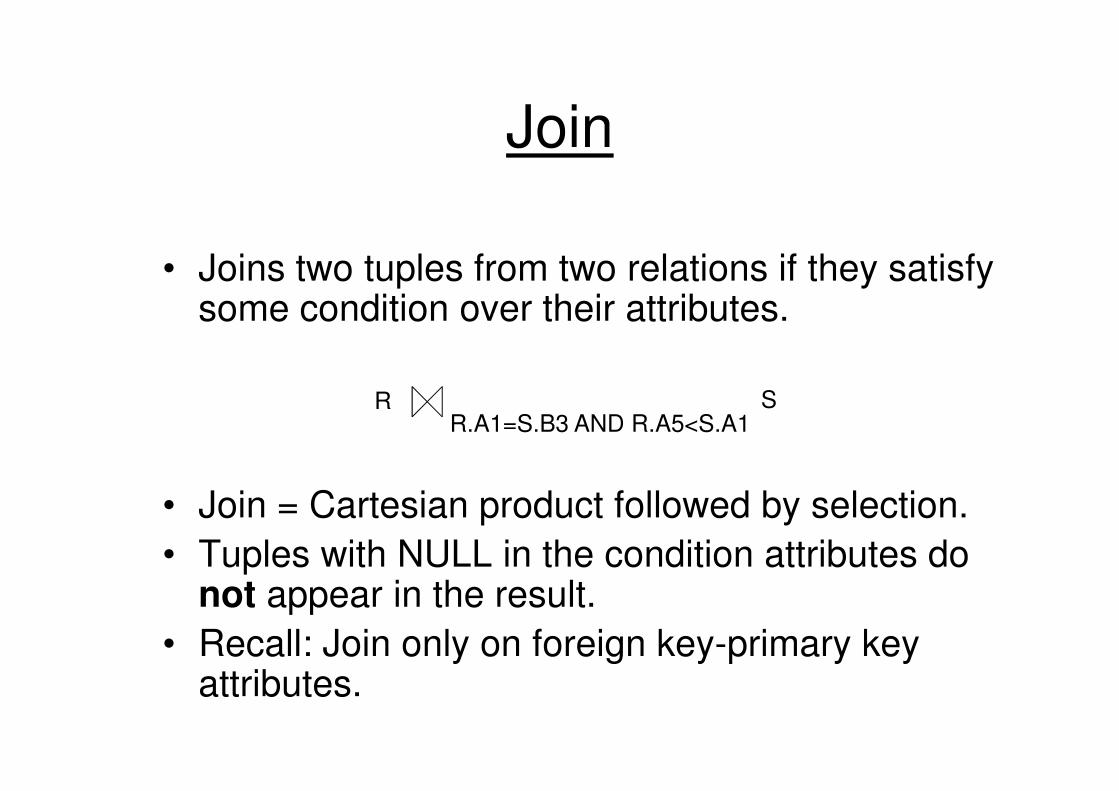
Join
• Joins two tuples from two relations if they satisfy some condition over their attributes.
R S
• Join = Cartesian product followed by selection.
• Tuples with NULL in the condition attributes do not appear in the result.
• Recall: Join only on foreign key-primary key attributes.
R.A1=S.B3 AND R.A5<S.A1R S

Example: join
Name STATE
Los Angeles Calif
Oakland Calif
Atlanta Ga
San Fransisco Calif
Key City
5 San Fransisco
7 Oakland
R:S:
San Fransisco Calif
Boston Mass
8 Boston
Name STATE Key City
Oakland Calif 7 Oakland
San Fransisco Calif 5 San Fransisco
Boston Mass 8 Boston
R.Name=S.CityR S

Name STATE Key City
Los Angeles Calif 5 San Fransisco
Los Angeles Calif 7 Oakland
Los Angeles Calif 8 Boston
Oakland Calif 5 San Fransisco
Oakland Calif 7 Oakland
Oakland Calif 8 Boston
Atlanta Ga 5 San FransiscoAtlanta Ga 5 San Fransisco
Atlanta Ga 7 Oakland
Atlanta Ga 8 Boston
San Fransisco Calif 5 San Fransisco
San Fransisco Calif 7 Oakland
San Fransisco Calif 8 Boston
Boston Mass 5 San Fransisco
Boston Mass 7 Oakland
Boston Mass 8 Boston

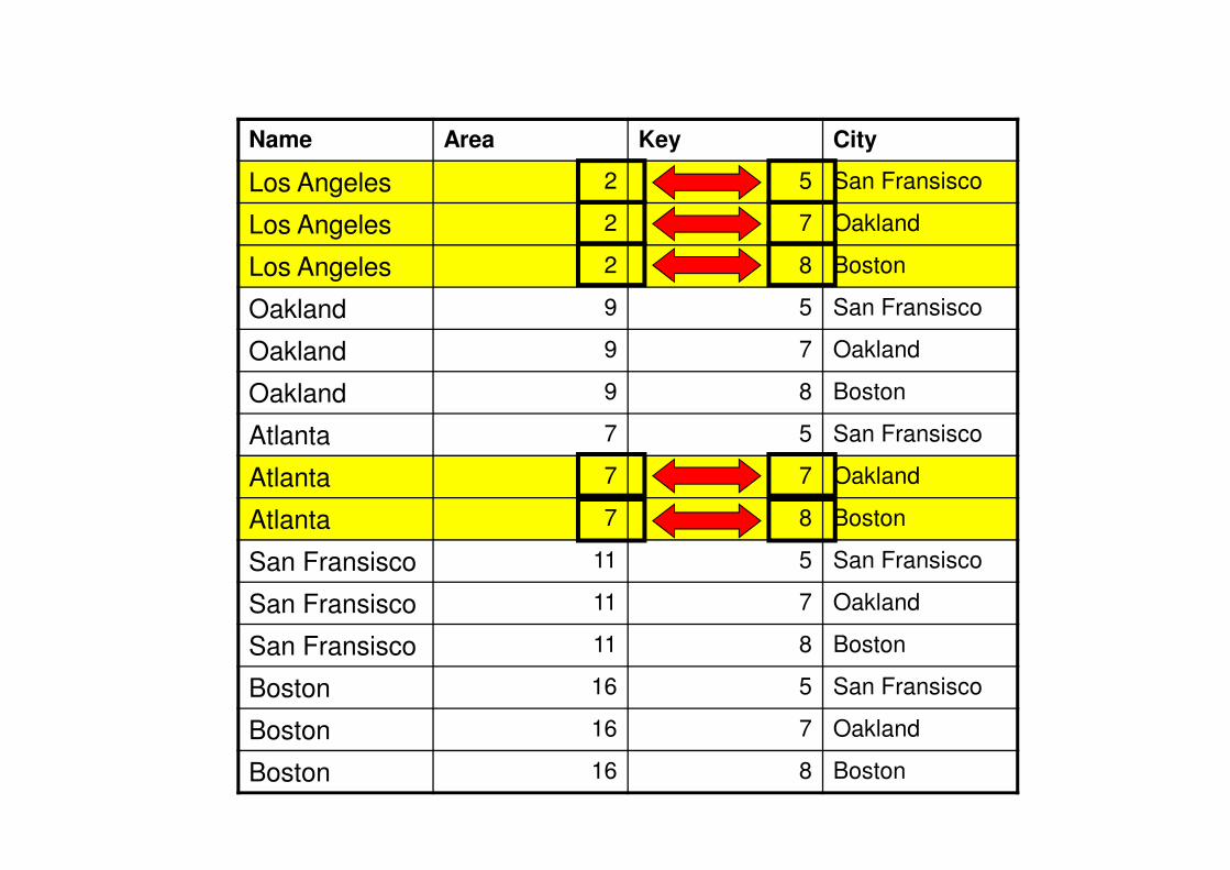
Example: join
Name Area
Los Angeles 2
Oakland 9
Atlanta 7
San Fransisco 11
R:
Name Area Key City
Los Angeles 2 5 San Fransisco
Los Angeles 2 7 Oakland
Los Angeles 2 8 Boston
Atlanta 7 7 OaklandSan Fransisco 11
Boston 16
Key City
5 San Fransisco
7 Oakland
8 Boston
S: R.Area<=S.KeyR S
Atlanta 7 7 Oakland
Atlanta 7 8 Boston
Name Area Key City
Los Angeles 2 5 San Fransisco
Los Angeles 2 7 Oakland
Los Angeles 2 8 Boston
Oakland 9 5 San Fransisco
Oakland 9 7 Oakland
Oakland 9 8 Boston
Atlanta 7 5 San FransiscoAtlanta 7 5 San Fransisco
Atlanta 7 7 Oakland
Atlanta 7 8 Boston
San Fransisco 11 5 San Fransisco
San Fransisco 11 7 Oakland
San Fransisco 11 8 Boston
Boston 16 5 San Fransisco
Boston 16 7 Oakland
Boston 16 8 Boston
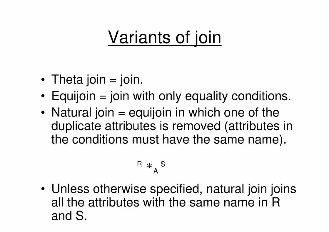
Variants of join
• Theta join = join.
• Equijoin = join with only equality conditions.
• Natural join = equijoin in which one of the • Natural join = equijoin in which one of the duplicate attributes is removed (attributes in the conditions must have the same name).
• Unless otherwise specified, natural join joins all the attributes with the same name in R and S.
AR S*
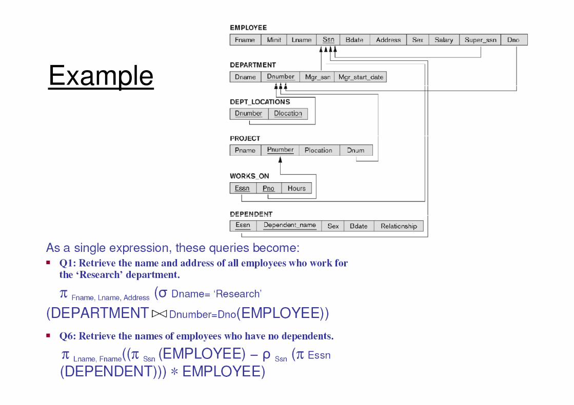
Example
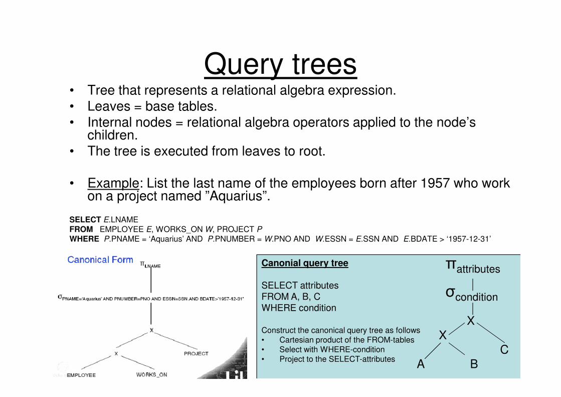
Query trees• Tree that represents a relational algebra expression.• Leaves = base tables.• Internal nodes = relational algebra operators applied to the node’s
children.• The tree is executed from leaves to root.
• Example: List the last name of the employees born after 1957 who work on a project named ”Aquarius”.on a project named ”Aquarius”.
SELECT E.LNAME
FROM EMPLOYEE E, WORKS_ON W, PROJECT P
WHERE P.PNAME = ‘Aquarius’ AND P.PNUMBER = W.PNO AND W.ESSN = E.SSN AND E.BDATE > ‘1957-12-31’
Canonial query tree
SELECT attributesFROM A, B, CWHERE condition
X
X
C
A B
σcondition
πattributes
Construct the canonical query tree as follows
• Cartesian product of the FROM-tables
• Select with WHERE-condition
• Project to the SELECT-attributes

Equivalent query trees
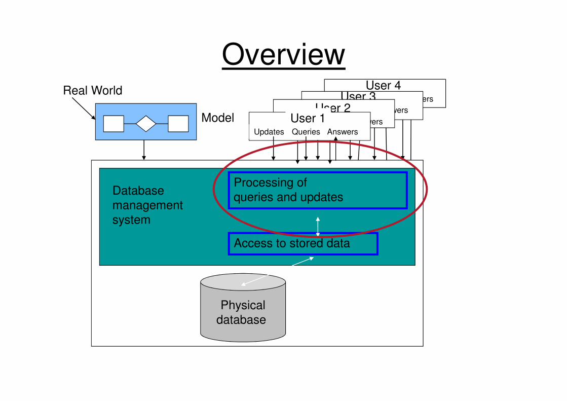
Real World
Model
Database
management
Processing of
queries and updates
Queries AnswersUpdates
User 4
Queries AnswersUpdates
User 3
Queries AnswersUpdates
User 2
Queries AnswersUpdates
User 1
Overview
Physical
database
management
system
queries and updates
Access to stored data
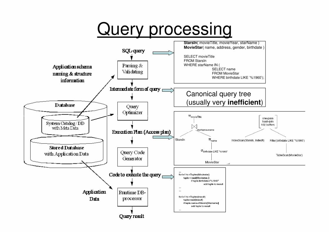
Query processingStarsIn( movieTitle, movieYear, starName )
MovieStar( name, address, gender, birthdate )
SELECT movieTitle
FROM StarsIn
WHERE starName IN (
SELECT name
FROM MovieStar
WHERE birthdate LIKE ’%1960’);
Canonical query tree
(usually very inefficient)
Parsing and validating
• Control of used relations
– Have to be declared in FROM
– Must exist in the database
• Control and resolve attributes• Control and resolve attributes
– Attributes must exist in the relations
• Type checking
– Attributes that are compared must be of the same type
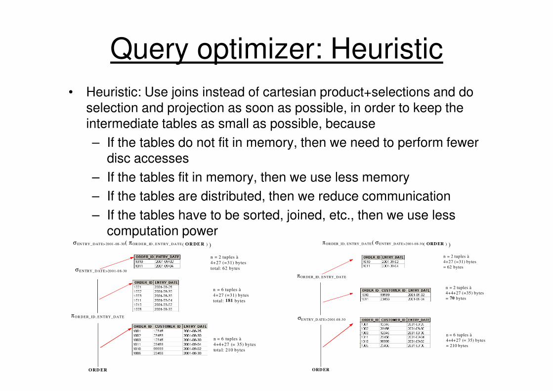
Query optimizer: Heuristic
• Heuristic: Use joins instead of cartesian product+selections and do selection and projection as soon as possible, in order to keep the intermediate tables as small as possible, because
– If the tables do not fit in memory, then we need to perform fewer disc accesses
– If the tables fit in memory, then we use less memory
– If the tables are distributed, then we reduce communication– If the tables are distributed, then we reduce communication
– If the tables have to be sorted, joined, etc., then we use less computation power
πOR DER_ID, ENTRY_DATE
σENTRY_DATE>2001-08-30
ORD ER
σENTRY_ DATE> 2001-08-30( πOR DER_ID , ENTRY_ DATE( OR DE R ) )
n = 6 tuples à
4+4+27 (= 35) bytes
tota l: 210 bytes
n = 6 tuples à
4+27 (=31) bytes
total: 181 bytes
n = 2 tuples à
4+27 (=31) bytes
total: 62 bytes
πOR DER_ID, ENTRY_DATE
σENTRY_D ATE>2001-08-30
ORD ER
πOR DER_ID, ENTRY_DATE( σENTRY _DATE>2001-08-30( ORD ER ) )
n = 6 tuples à
4+4+27 (= 35) bytes
= 210 bytes
n = 2 tuples à
4+4+27 (=35) bytes
= 70 bytes
n = 2 tuples à
4+27 (=31) bytes
= 62 bytes
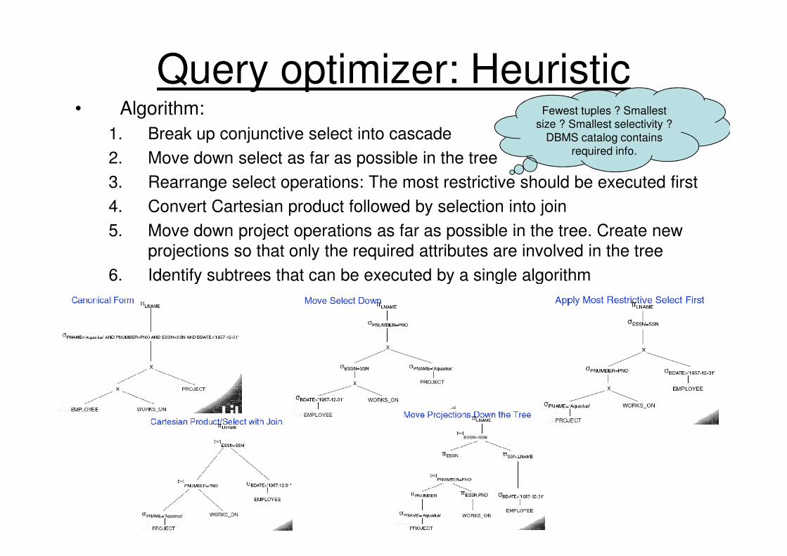
Query optimizer: Heuristic• Algorithm:
1. Break up conjunctive select into cascade
2. Move down select as far as possible in the tree
3. Rearrange select operations: The most restrictive should be executed first
4. Convert Cartesian product followed by selection into join
5. Move down project operations as far as possible in the tree. Create new
projections so that only the required attributes are involved in the tree
6. Identify subtrees that can be executed by a single algorithm
Fewest tuples ? Smallest
size ? Smallest selectivity ?
DBMS catalog contains
required info.
6. Identify subtrees that can be executed by a single algorithm
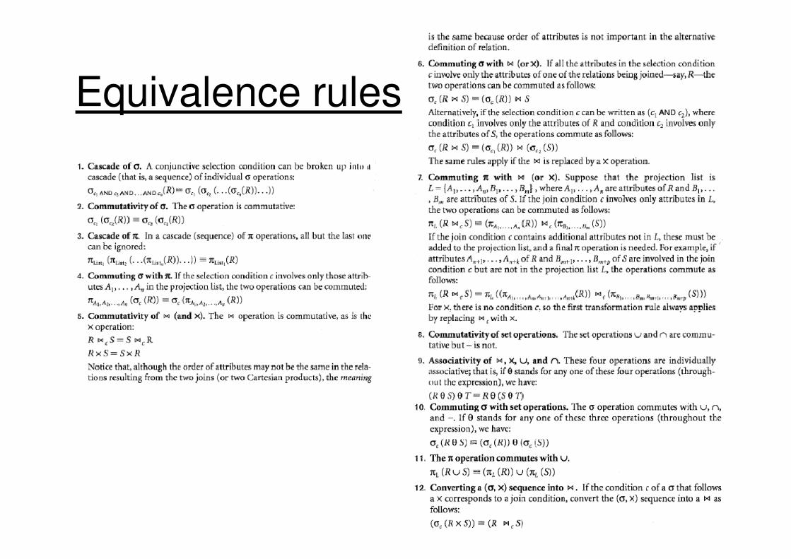
Equivalence rules
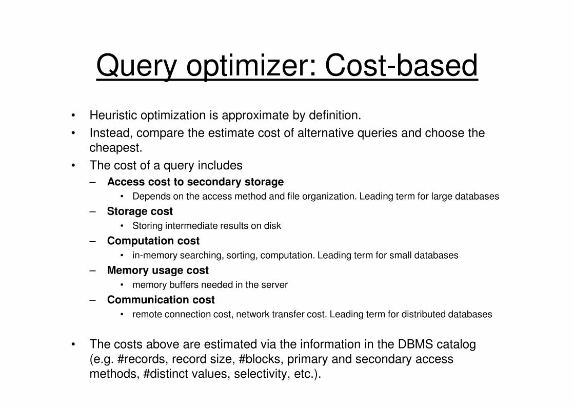
Query optimizer: Cost-based
• Heuristic optimization is approximate by definition.
• Instead, compare the estimate cost of alternative queries and choose the
cheapest.
• The cost of a query includes
– Access cost to secondary storage
• Depends on the access method and file organization. Leading term for large databases
– Storage cost
• Storing intermediate results on disk
– Computation cost
• in-memory searching, sorting, computation. Leading term for small databases
– Memory usage cost
• memory buffers needed in the server
– Communication cost
• remote connection cost, network transfer cost. Leading term for distributed databases
• The costs above are estimated via the information in the DBMS catalog
(e.g. #records, record size, #blocks, primary and secondary access
methods, #distinct values, selectivity, etc.).
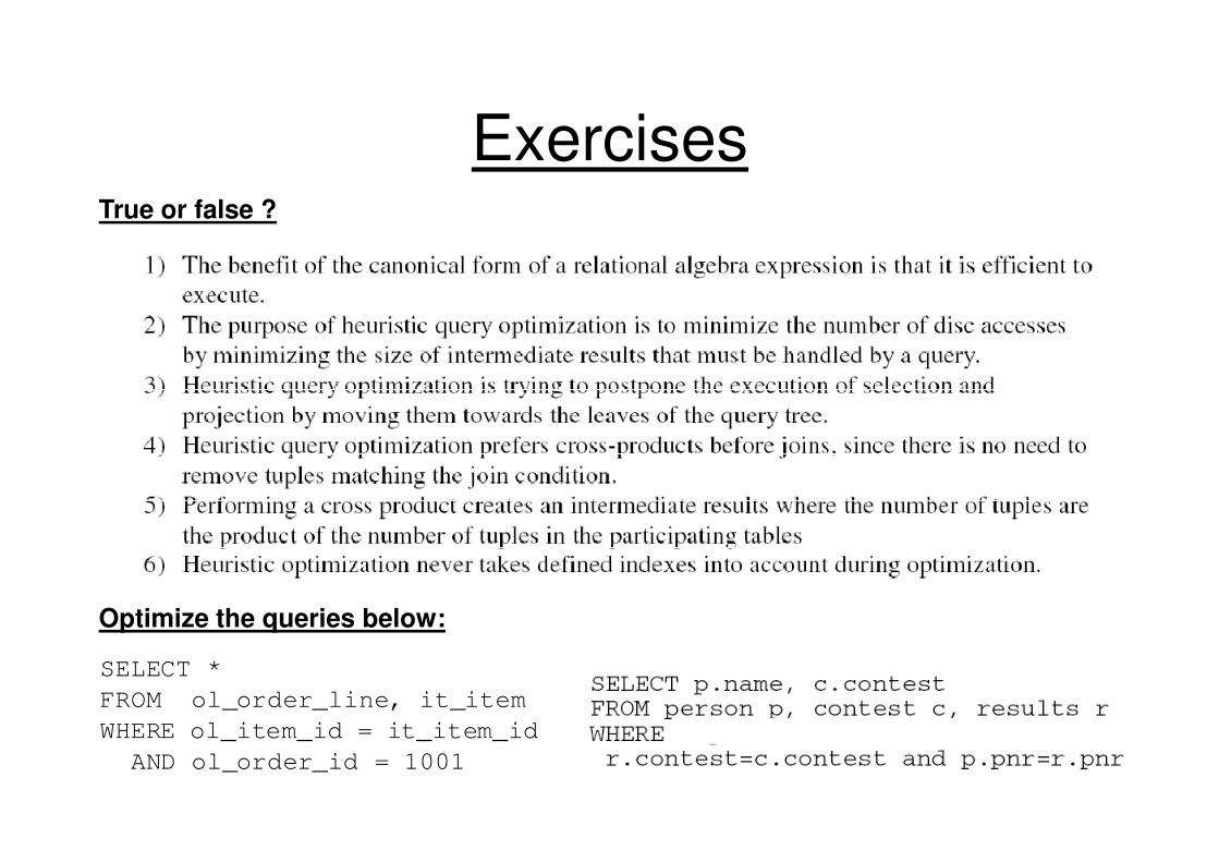
ExercisesTrue or false ?
SELECT *
FROM ol_order_line, it_item
WHERE ol_item_id = it_item_id
AND ol_order_id = 1001
Optimize the queries below:
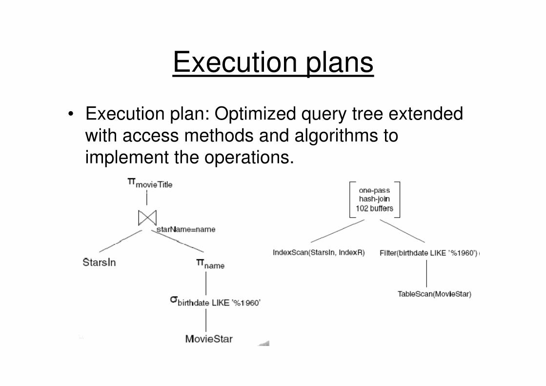
Execution plans
• Execution plan: Optimized query tree extended
with access methods and algorithms to
implement the operations.


