Download - Q922+re2+l07 v1

Reservoir Engineering 2 Course (1st Ed.)

mailto:[email protected]

http://bit.ly/Q922-RE2

mailto:[email protected]

http://bit.ly/Q922-RE2

1. Water Influx ModelsA. The Pot Aquifer Model

B. Schilthuis’ SS Model

C. Hurst’s Modified SS Model

1. mathematical Water Influx models;A. The van Everdingen-Hurst Unsteady-State Model

a. Edge-Water DriveI. computational steps for We at successive intervals

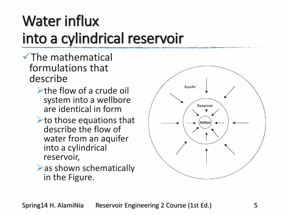
Water influx into a cylindrical reservoirThe mathematical

formulations that describe the flow of a crude oil

system into a wellbore are identical in form

to those equations that describe the flow of water from an aquifer into a cylindrical reservoir,

as shown schematically in the Figure.

Spring14 H. AlamiNia Reservoir Engineering 2 Course (1st Ed.) 5

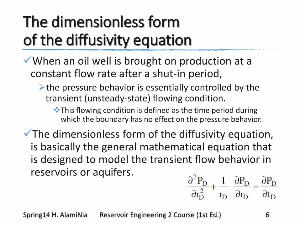
The dimensionless form of the diffusivity equationWhen an oil well is brought on production at a

constant flow rate after a shut-in period, the pressure behavior is essentially controlled by the

transient (unsteady-state) flowing condition. This flowing condition is defined as the time period during

which the boundary has no effect on the pressure behavior.

The dimensionless form of the diffusivity equation, is basically the general mathematical equation that is designed to model the transient flow behavior in reservoirs or aquifers.


Van Everdingen and Hurst (1949) solutionsVan Everdingen and Hurst (1949) proposed

solutions to the dimensionless diffusivity equation for the two reservoir-aquifer boundary conditions:Constant terminal rate

For the constant-terminal-rate boundary condition, the rate of water influx is assumed constant for a given period; and the pressure drop at the reservoir-aquifer boundary is calculated.

Constant terminal pressureFor the constant-terminal-pressure boundary condition,

a boundary pressure drop is assumed constant over some finite time period, and the water influx rate is determined.


Constant terminal pressure solution

In the description of water influx from an aquifer into a reservoir, there is greater interest in calculating the influx rate rather than the pressure. This leads to the determination of the water influx

as a function of a given pressure drop at the inner boundary of the reservoir-aquifer system.

Van Everdingen and Hurst solved the diffusivity equation for the aquifer-reservoir system by applying the Laplace transformation to the equation. The authors’ solution can be used to determine the

water influx in the following systems:Edge-water-drive system (radial system)Bottom-water-drive systemLinear-water-drive system


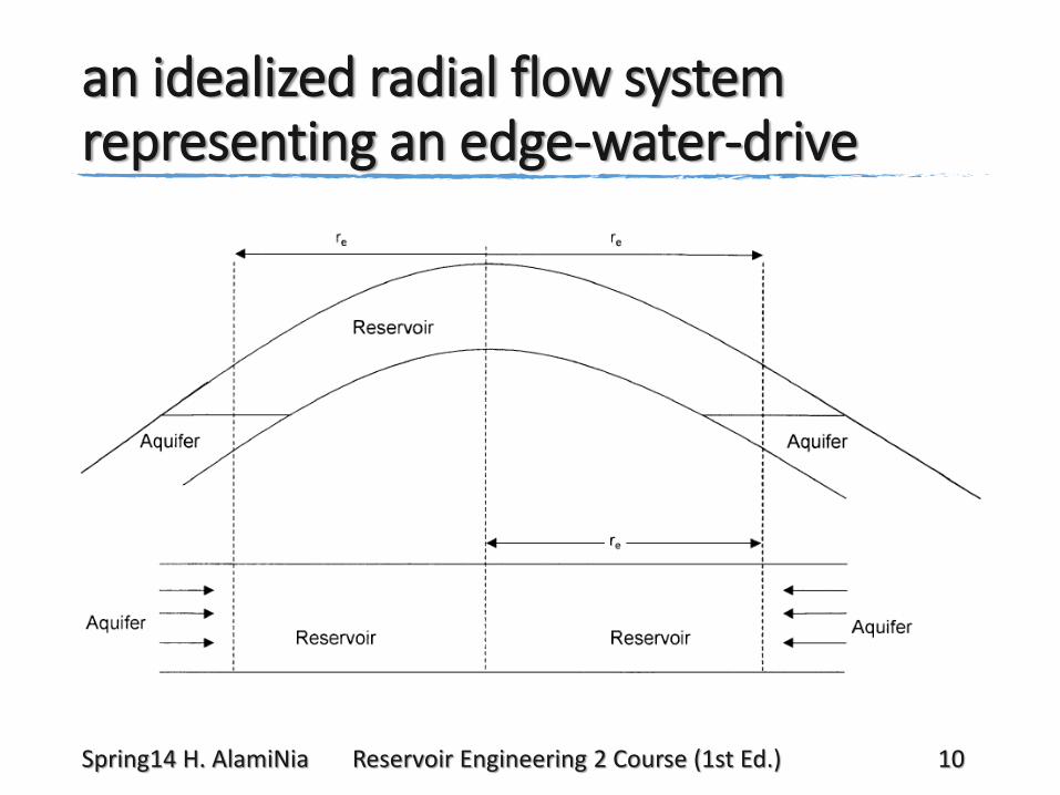
an idealized radial flow system representing an edge-water-drive


an idealized radial flow system representing an edge-water-driveIn previous slide:

The inner boundary is defined as the interface between the reservoir and the aquifer.

The flow across this inner boundary is considered horizontal and encroachment occurs across a cylindrical plane encircling the reservoir.

With the interface as the inner boundary, it is possible to impose a constant terminal pressure at the inner boundary and determine the rate of water influx across the interface.


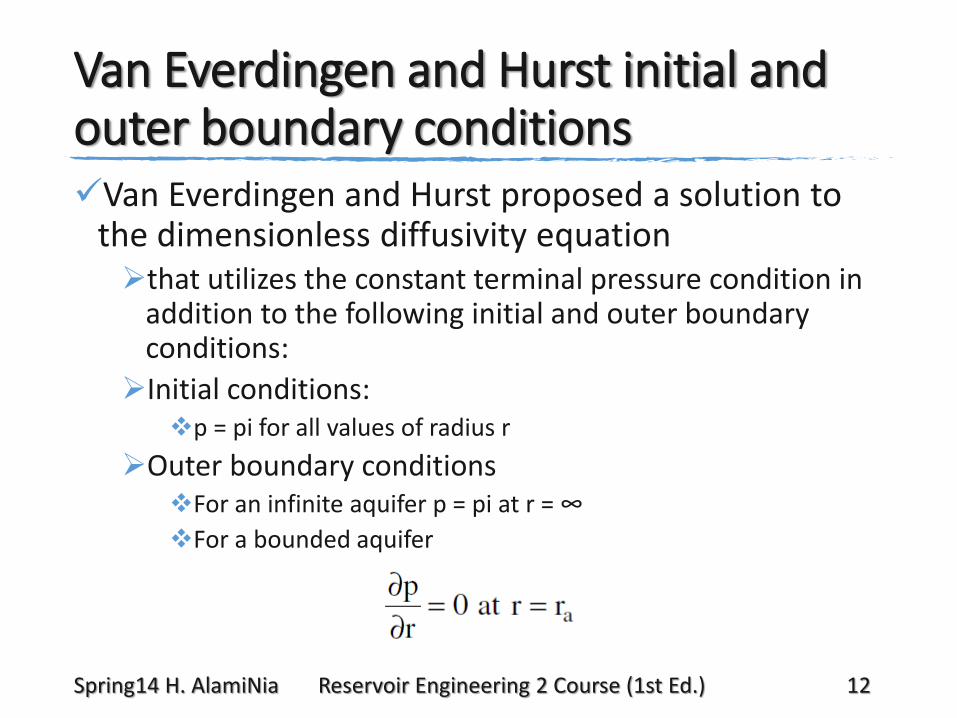
Van Everdingen and Hurst initial and outer boundary conditionsVan Everdingen and Hurst proposed a solution to

the dimensionless diffusivity equation that utilizes the constant terminal pressure condition in

addition to the following initial and outer boundary conditions:

Initial conditions:p = pi for all values of radius r

Outer boundary conditionsFor an infinite aquifer p = pi at r = ∞

For a bounded aquifer


Van Everdingen and Hurst assumption

Van Everdingen and Hurst assumed that the aquifer is characterized by:Uniform thickness

Constant permeability (k=constant)

Uniform porosity (phi)

Constant rock compressibility

Constant water compressibility


dimensionless water influx

The authors expressed their mathematical relationship for calculating the water influx in a form of a dimensionless parameter that is called dimensionless water influx

WeD.

They also expressed the dimensionless water influx as a function of the dimensionless time tD

and dimensionless radius rD,

thus they made the

solution to the diffusivity equation generalized and applicable to any aquifer where the

flow of water into the reservoir is essentially radial.

The solutions were derived for cases of bounded aquifers and

aquifers of infinite extent.

The authors presented their solution in tabulated and graphical forms.


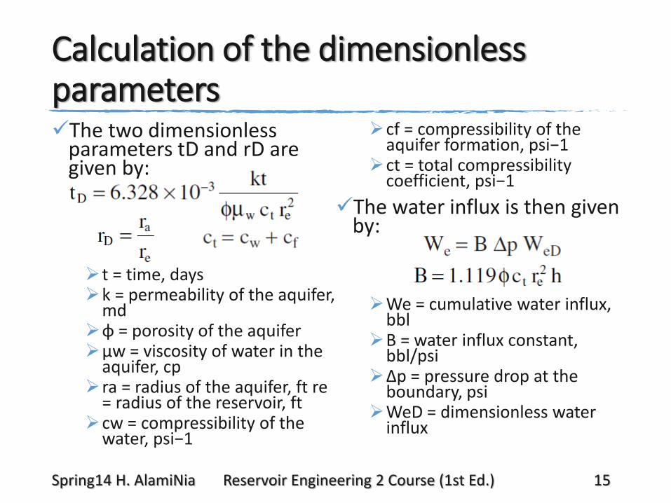
Calculation of the dimensionless parametersThe two dimensionless

parameters tD and rD are given by:

t = time, days k = permeability of the aquifer,

md φ = porosity of the aquifer μw = viscosity of water in the

aquifer, cpra = radius of the aquifer, ft re

= radius of the reservoir, ftcw = compressibility of the

water, psi−1

cf = compressibility of the aquifer formation, psi−1

ct = total compressibility coefficient, psi−1

The water influx is then given by:

We = cumulative water influx, bbl

B = water influx constant, bbl/psi

Δp = pressure drop at the boundary, psi

WeD = dimensionless water influx


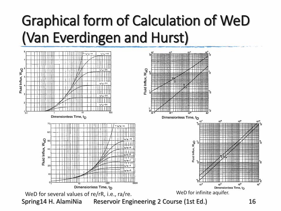
Graphical form of Calculation of WeD (Van Everdingen and Hurst)

WeD for several values of re/rR, i.e., ra/re. WeD for infinite aquifer.


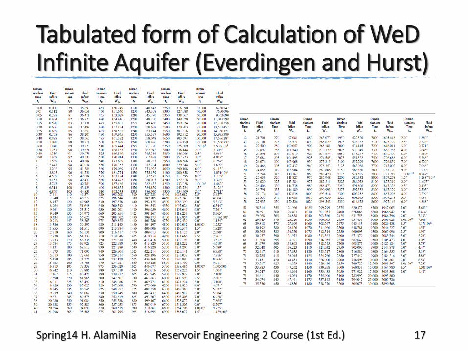
Tabulated form of Calculation of WeD Infinite Aquifer (Everdingen and Hurst)


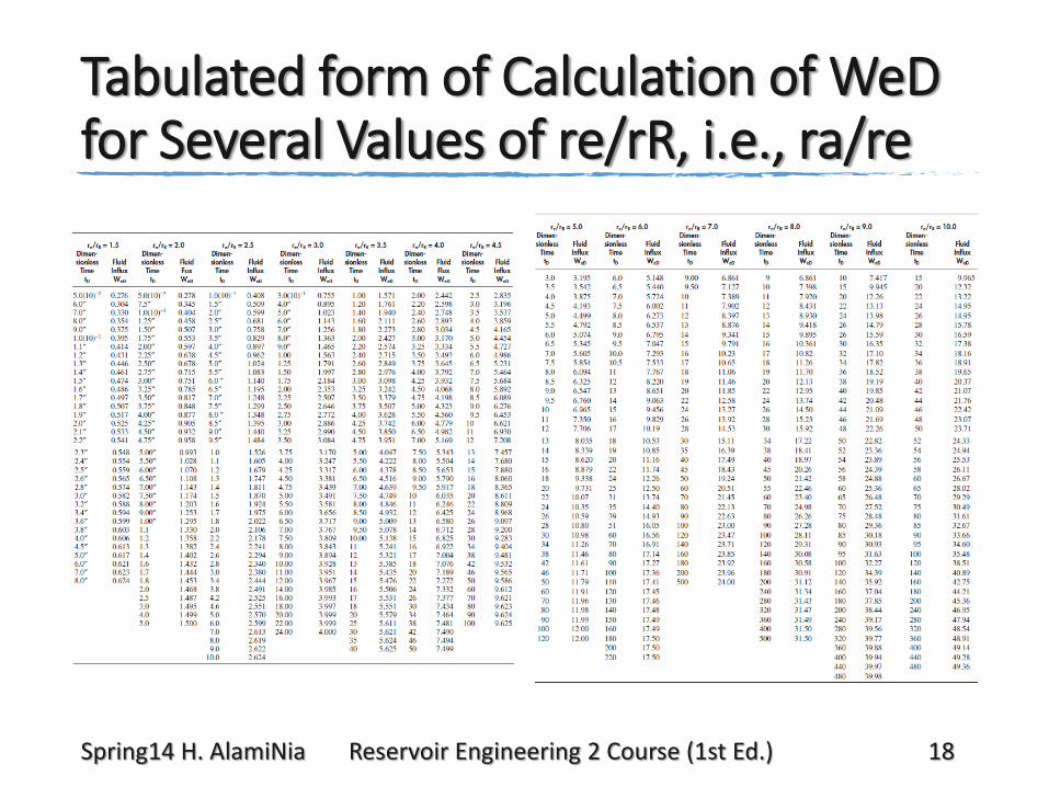
Tabulated form of Calculation of WeD for Several Values of re/rR, i.e., ra/re


not circular water encroachment

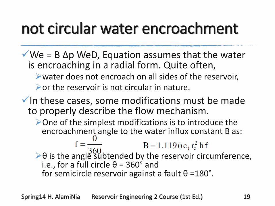
We = B Δp WeD, Equation assumes that the water is encroaching in a radial form. Quite often, water does not encroach on all sides of the reservoir, or the reservoir is not circular in nature.

In these cases, some modifications must be made to properly describe the flow mechanism. One of the simplest modifications is to introduce the

encroachment angle to the water influx constant B as:

θ is the angle subtended by the reservoir circumference, i.e., for a full circle θ = 360° and for semicircle reservoir against a fault θ =180°.


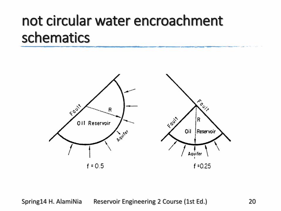
not circular water encroachment schematics


cumulative water influx calculation at successive intervalsIn order to determine the total water influx into a

reservoir at any given time, it is necessary to determine the water influx as a result of each successive pressure drop that has been imposed on the reservoir and aquifer.

In calculating cumulative water influx into a reservoir at successive intervals, it is necessary to calculate the total water influx from the beginning. This is required because of the different times during

which the various pressure drops have been effective.


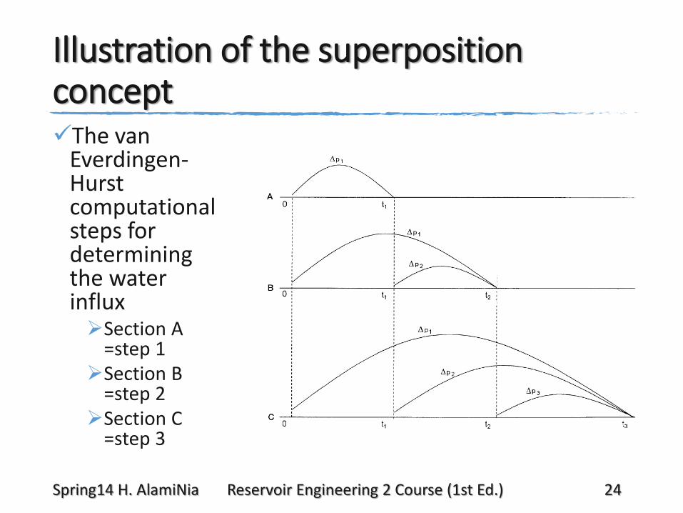
Illustration of the superposition conceptThe van

Everdingen-Hurst computational steps for determining the water influxSection A

=step 1Section B

=step 2Section C

=step 3


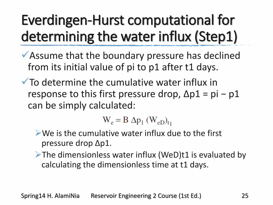
Everdingen-Hurst computational for determining the water influx (Step1)Assume that the boundary pressure has declined

from its initial value of pi to p1 after t1 days.

To determine the cumulative water influx in response to this first pressure drop, Δp1 = pi − p1 can be simply calculated:

We is the cumulative water influx due to the first pressure drop Δp1.

The dimensionless water influx (WeD)t1 is evaluated by calculating the dimensionless time at t1 days.


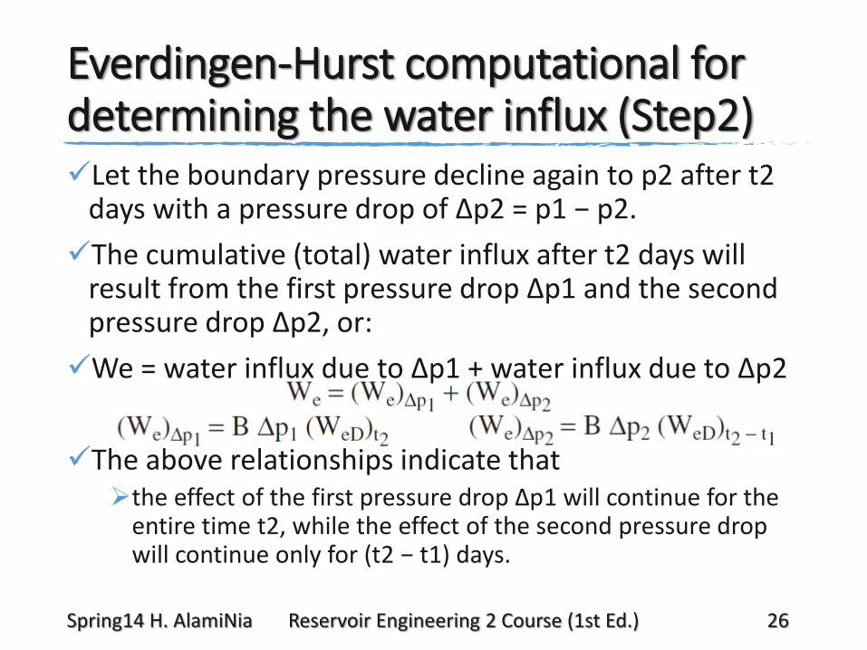
Everdingen-Hurst computational for determining the water influx (Step2)Let the boundary pressure decline again to p2 after t2

days with a pressure drop of Δp2 = p1 − p2.

The cumulative (total) water influx after t2 days will result from the first pressure drop Δp1 and the second pressure drop Δp2, or:

We = water influx due to Δp1 + water influx due to Δp2

The above relationships indicate that the effect of the first pressure drop Δp1 will continue for the

entire time t2, while the effect of the second pressure drop will continue only for (t2 − t1) days.


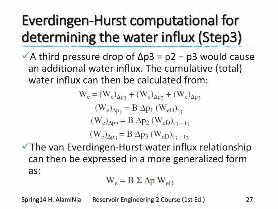
Everdingen-Hurst computational for determining the water influx (Step3)A third pressure drop of Δp3 = p2 − p3 would cause

an additional water influx. The cumulative (total) water influx can then be calculated from:

The van Everdingen-Hurst water influx relationship can then be expressed in a more generalized form as:


pressure drop modification

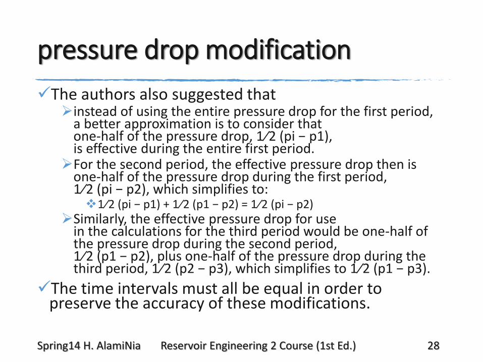
The authors also suggested that instead of using the entire pressure drop for the first period,

a better approximation is to consider that one-half of the pressure drop, 1⁄2 (pi − p1), is effective during the entire first period.

For the second period, the effective pressure drop then is one-half of the pressure drop during the first period, 1⁄2 (pi − p2), which simplifies to:1⁄2 (pi − p1) + 1⁄2 (p1 − p2) = 1⁄2 (pi − p2)

Similarly, the effective pressure drop for use in the calculations for the third period would be one-half of the pressure drop during the second period, 1⁄2 (p1 − p2), plus one-half of the pressure drop during the third period, 1⁄2 (p2 − p3), which simplifies to 1⁄2 (p1 − p3).

The time intervals must all be equal in order to preserve the accuracy of these modifications.


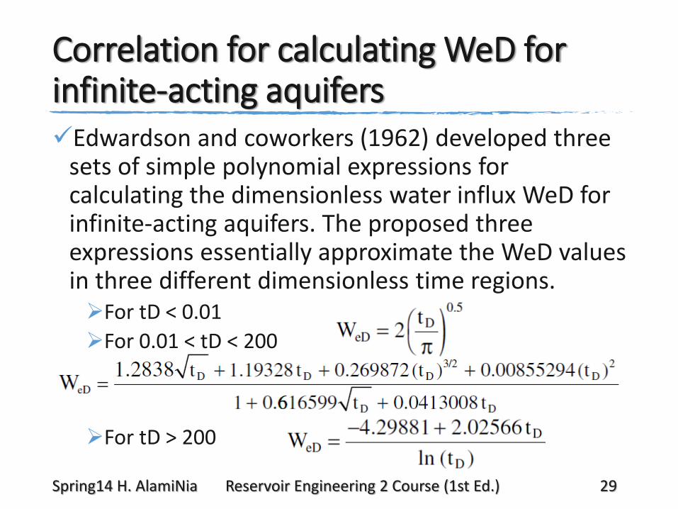
Correlation for calculating WeD for infinite-acting aquifersEdwardson and coworkers (1962) developed three

sets of simple polynomial expressions for calculating the dimensionless water influx WeD for infinite-acting aquifers. The proposed three expressions essentially approximate the WeD values in three different dimensionless time regions.For tD < 0.01

For 0.01 < tD < 200

For tD > 200


1. Ahmed, T. (2010). Reservoir engineering handbook (Gulf Professional Publishing). Chapter 10

1. mathematical Water Influx models;A. The van Everdingen-Hurst Unsteady-State Model

bottom-Water Drive

B. The Carter-Tracy Water Influx Model

C. Fetkovich’s Method

Download - Q922+re2+l07 v1

Top Related