Download - Q921 re1 lec11 v1

Reservoir Engineering 1 Course (2nd Ed.)

mailto:[email protected]

http://bit.ly/Q921-RE1

mailto:[email protected]

http://bit.ly/Q921-RE1

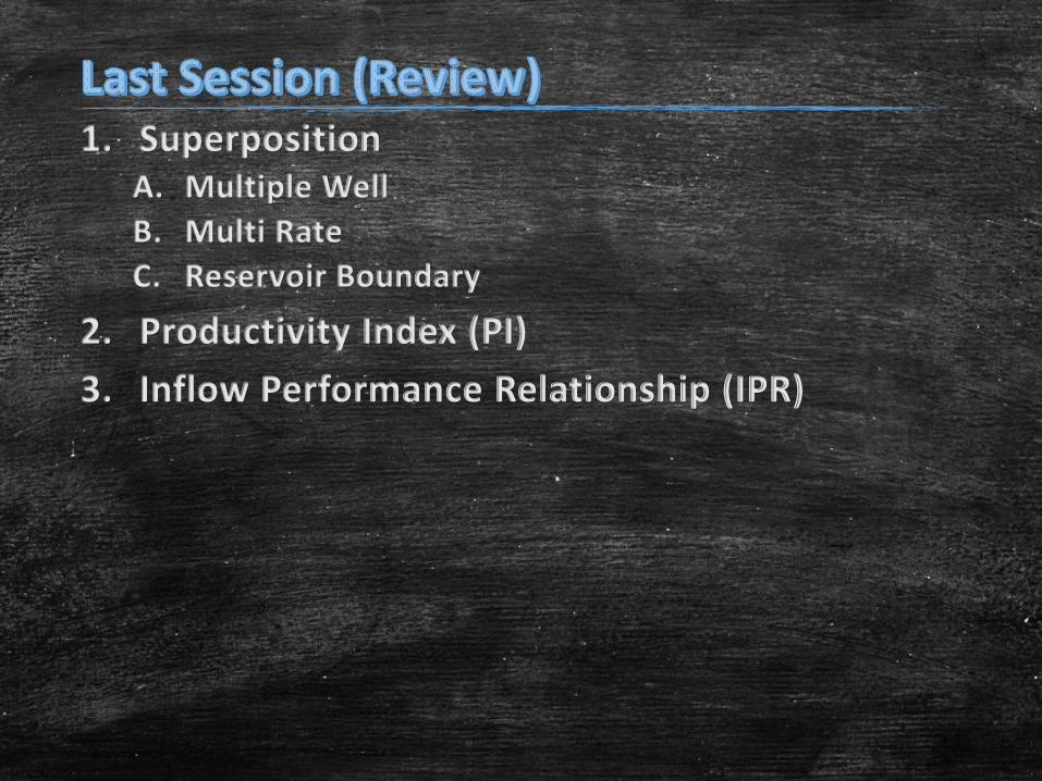
1. SuperpositionA. Multiple Well

B. Multi Rate

C. Reservoir Boundary

2. Productivity Index (PI)

3. Inflow Performance Relationship (IPR)

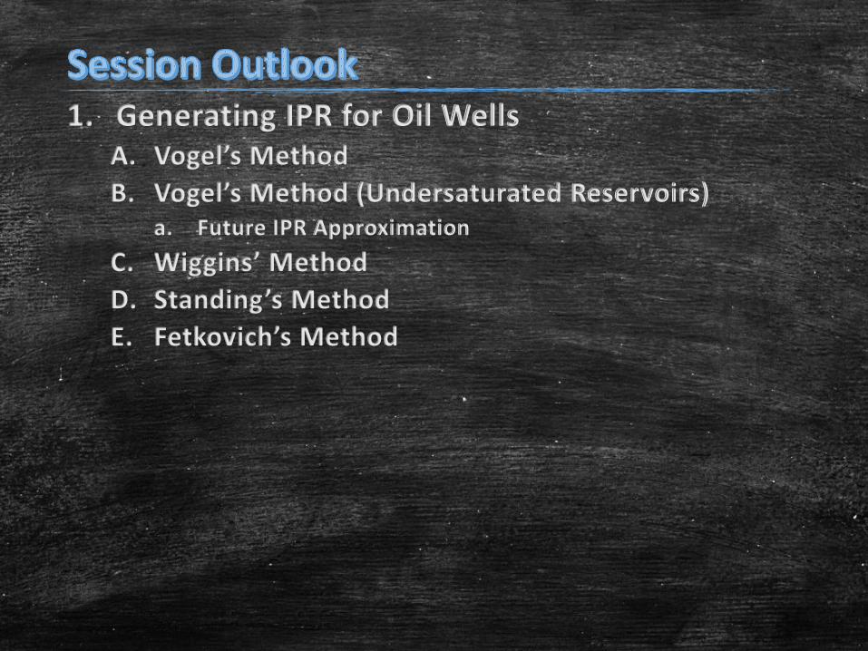
1. Generating IPR for Oil WellsA. Vogel’s Method

B. Vogel’s Method (Undersaturated Reservoirs)a. Future IPR Approximation

C. Wiggins’ Method

D. Standing’s Method

E. Fetkovich’s Method

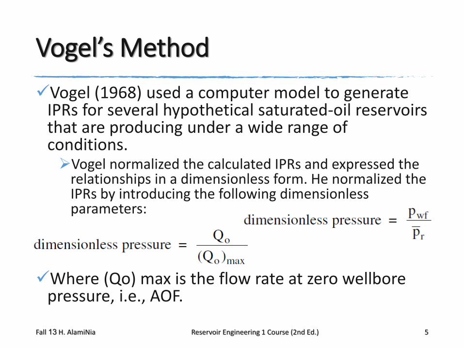
Vogel’s Method

Vogel (1968) used a computer model to generate IPRs for several hypothetical saturated-oil reservoirs that are producing under a wide range of conditions.Vogel normalized the calculated IPRs and expressed the

relationships in a dimensionless form. He normalized the IPRs by introducing the following dimensionless parameters:

Where (Qo) max is the flow rate at zero wellbore pressure, i.e., AOF.

Fall 13 H. AlamiNia Reservoir Engineering 1 Course (2nd Ed.) 5

Vogel’s IPR

Vogel plotted the dimensionless IPR curves for all the reservoir cases and arrived at the following relationship between the above dimensionless parameters:

Where Qo = oil rate at pwf

(Qo) max = maximum oil flow rate at zero wellbore pressure, i.e., AOF

p–r = current average reservoir pressure, psig

pwf = wellbore pressure, psig

Notice that pwf and p–r must be expressed in psig.


Vogel’s Method for Comingle Production of Water and OilVogel’s method can be extended to account for

water production by replacing the dimensionless rate with QL/(QL) max where QL = Qo + Qw.This has proved to be valid for wells producing at water

cuts as high as 97%.

The method requires the following data:Current average reservoir pressure p–r

Bubble-point pressure pb

Stabilized flow test data that include Qo at pwf


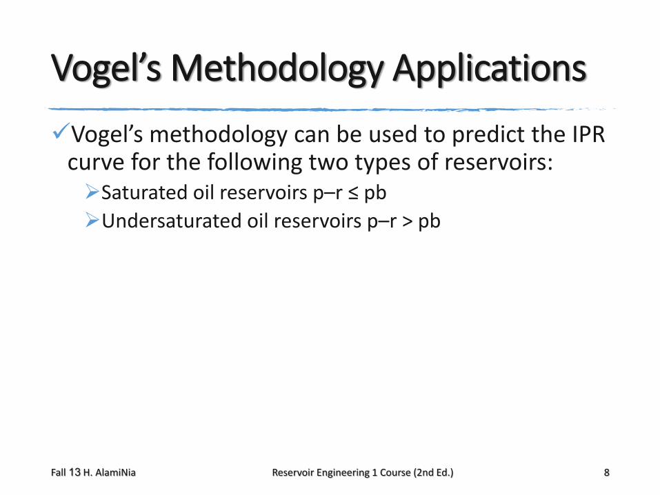
Vogel’s Methodology Applications

Vogel’s methodology can be used to predict the IPR curve for the following two types of reservoirs:Saturated oil reservoirs p–r ≤ pb

Undersaturated oil reservoirs p–r > pb


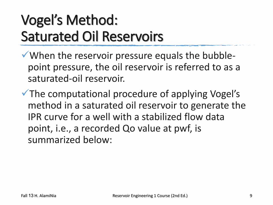
Vogel’s Method: Saturated Oil ReservoirsWhen the reservoir pressure equals the bubble-

point pressure, the oil reservoir is referred to as a saturated-oil reservoir.

The computational procedure of applying Vogel’s method in a saturated oil reservoir to generate the IPR curve for a well with a stabilized flow data point, i.e., a recorded Qo value at pwf, is summarized below:


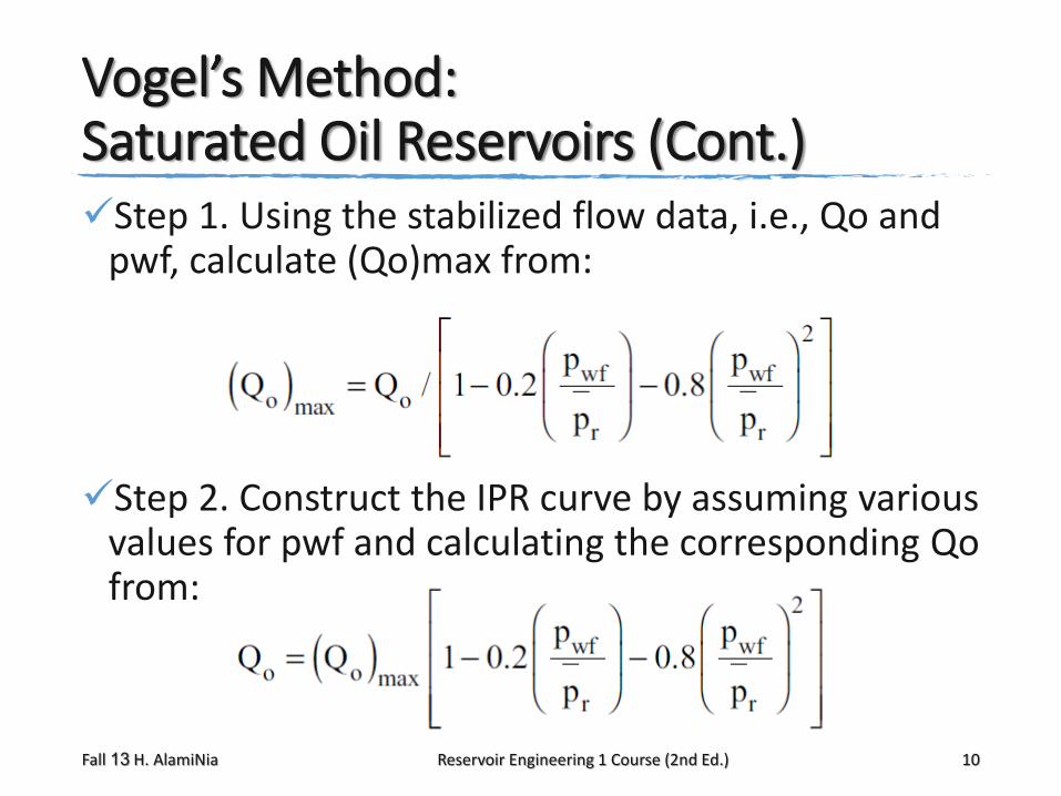
Vogel’s Method: Saturated Oil Reservoirs (Cont.)Step 1. Using the stabilized flow data, i.e., Qo and

pwf, calculate (Qo)max from:

Step 2. Construct the IPR curve by assuming various values for pwf and calculating the corresponding Qo from:


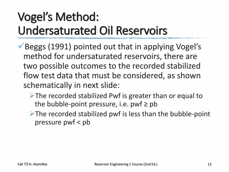
Vogel’s Method: Undersaturated Oil ReservoirsBeggs (1991) pointed out that in applying Vogel’s

method for undersaturated reservoirs, there are two possible outcomes to the recorded stabilized flow test data that must be considered, as shown schematically in next slide:The recorded stabilized Pwf is greater than or equal to

the bubble-point pressure, i.e. pwf ≥ pb

The recorded stabilized pwf is less than the bubble-point pressure pwf < pb


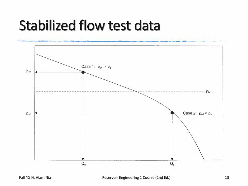
Stabilized flow test data


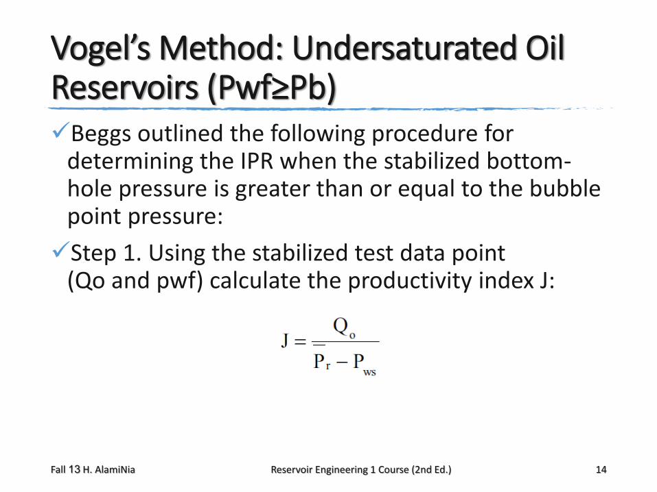
Vogel’s Method: Undersaturated Oil Reservoirs (Pwf≥Pb)Beggs outlined the following procedure for

determining the IPR when the stabilized bottom-hole pressure is greater than or equal to the bubble point pressure:

Step 1. Using the stabilized test data point (Qo and pwf) calculate the productivity index J:


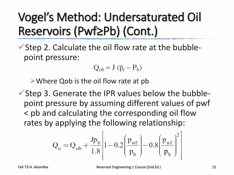
Vogel’s Method: Undersaturated Oil Reservoirs (Pwf≥Pb) (Cont.)Step 2. Calculate the oil flow rate at the bubble-

point pressure:

Where Qob is the oil flow rate at pb

Step 3. Generate the IPR values below the bubble-point pressure by assuming different values of pwf < pb and calculating the corresponding oil flow rates by applying the following relationship:


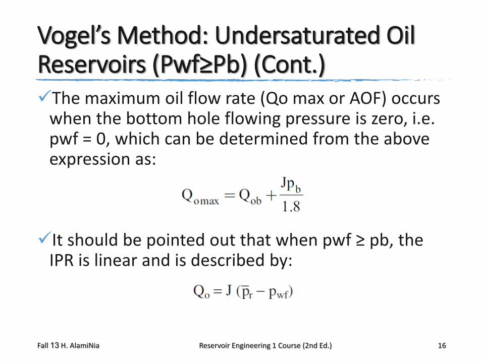
Vogel’s Method: Undersaturated Oil Reservoirs (Pwf≥Pb) (Cont.)The maximum oil flow rate (Qo max or AOF) occurs

when the bottom hole flowing pressure is zero, i.e. pwf = 0, which can be determined from the above expression as:

It should be pointed out that when pwf ≥ pb, the IPR is linear and is described by:


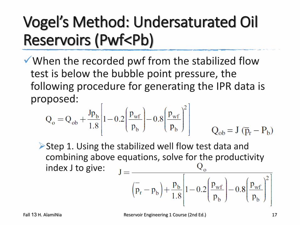
Vogel’s Method: Undersaturated Oil Reservoirs (Pwf<Pb)When the recorded pwf from the stabilized flow

test is below the bubble point pressure, the following procedure for generating the IPR data is proposed:

Step 1. Using the stabilized well flow test data and combining above equations, solve for the productivity index J to give:


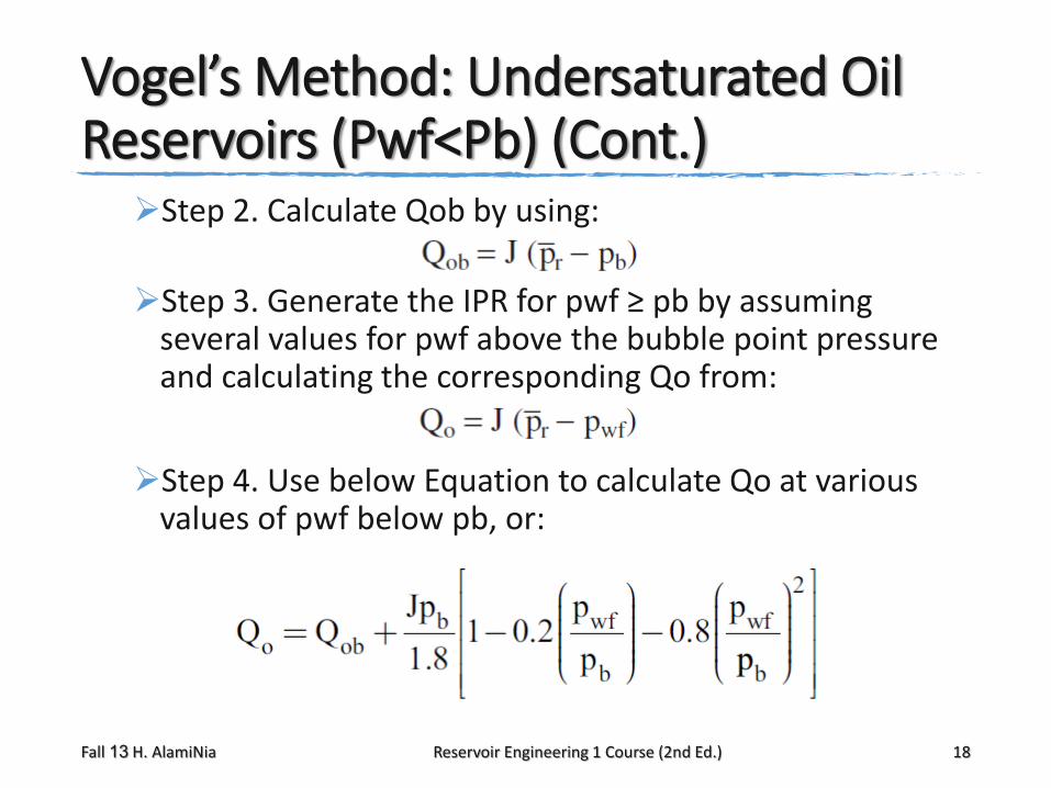
Vogel’s Method: Undersaturated Oil Reservoirs (Pwf<Pb) (Cont.)

Step 2. Calculate Qob by using:

Step 3. Generate the IPR for pwf ≥ pb by assuming several values for pwf above the bubble point pressure and calculating the corresponding Qo from:

Step 4. Use below Equation to calculate Qo at various values of pwf below pb, or:


IPR Prediction

Quite often it is necessary to predict the well’s inflow performance for future times as the reservoir pressure declines.

Future well performance calculations require the development of a relationship that can be used to predict future maximum oil flow rates.

Several methods are designed to address the problem of how the IPR might shift as the reservoir pressure declines.


IPR Prediction (Cont.)

Some of these prediction methods require the application of the material balance equation to generate future oil saturation data as a function of reservoir pressure. In the absence of such data, there are two simple

approximation methods that can be used in conjunction with Vogel’s method to predict future IPRs.


IPR Prediction: 1st Approximation Method This method provides a rough approximation of the

future maximum oil flow rate (Qomax)f at the specified future average reservoir pressure (pr)f. This future maximum flow rate (Qomax) f can be used in

Vogel’s equation to predict the future inflow performance relationships at (p–r)f.


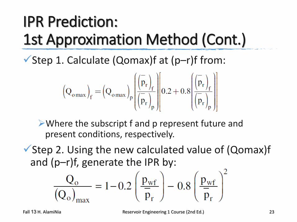
IPR Prediction: 1st Approximation Method (Cont.)Step 1. Calculate (Qomax)f at (p–r)f from:

Where the subscript f and p represent future and present conditions, respectively.

Step 2. Using the new calculated value of (Qomax)f and (p–r)f, generate the IPR by:


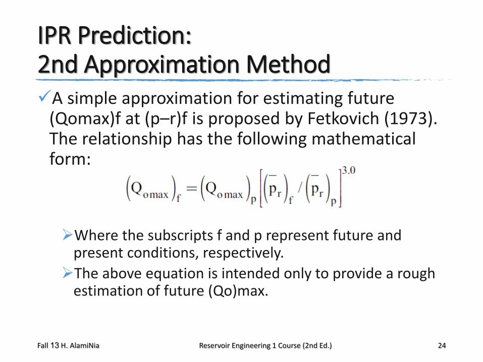
IPR Prediction: 2nd Approximation Method A simple approximation for estimating future

(Qomax)f at (p–r)f is proposed by Fetkovich (1973). The relationship has the following mathematical form:

Where the subscripts f and p represent future and present conditions, respectively.

The above equation is intended only to provide a rough estimation of future (Qo)max.


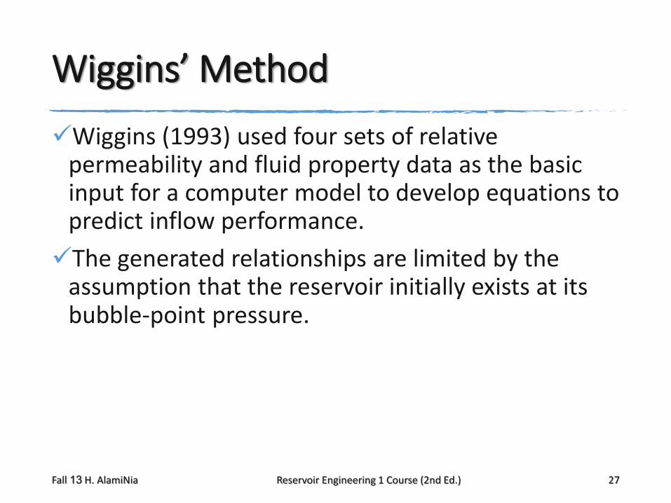
Wiggins’ Method

Wiggins (1993) used four sets of relative permeability and fluid property data as the basic input for a computer model to develop equations to predict inflow performance.

The generated relationships are limited by the assumption that the reservoir initially exists at its bubble-point pressure.


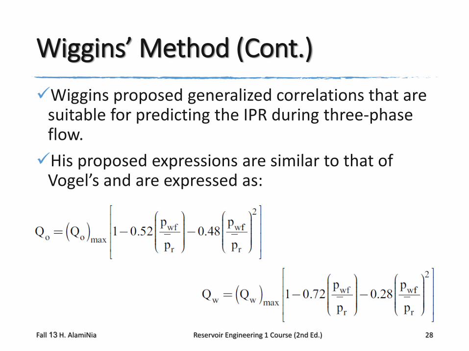
Wiggins’ Method (Cont.)

Wiggins proposed generalized correlations that are suitable for predicting the IPR during three-phase flow.

His proposed expressions are similar to that of Vogel’s and are expressed as:


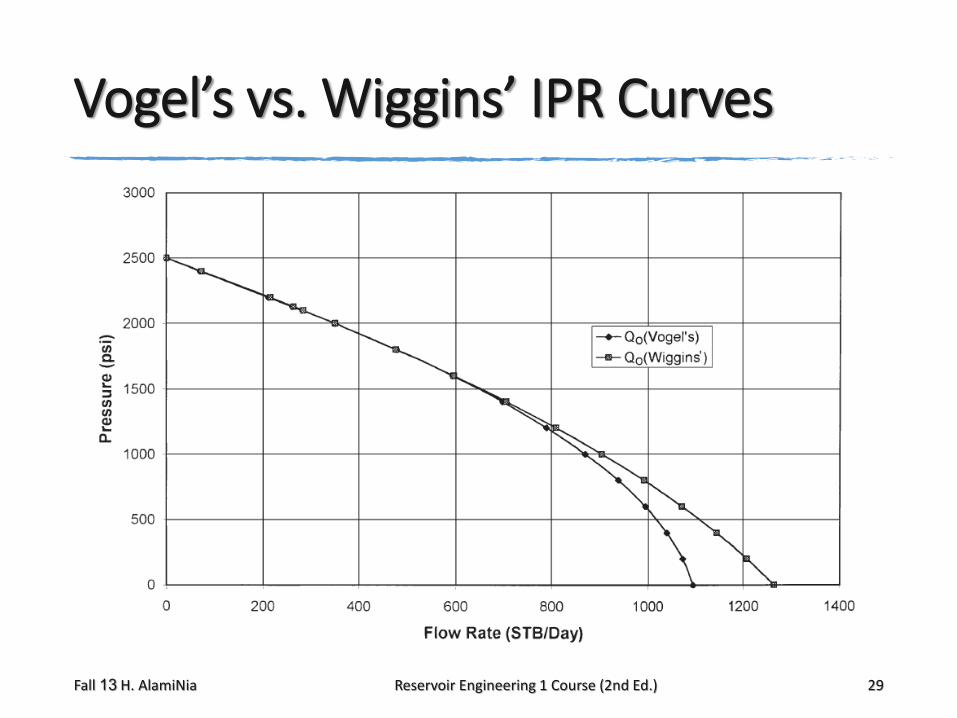
Vogel’s vs. Wiggins’ IPR Curves


Standing’s Method

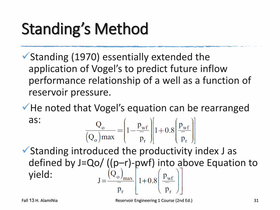
Standing (1970) essentially extended the application of Vogel’s to predict future inflow performance relationship of a well as a function of reservoir pressure.

He noted that Vogel’s equation can be rearranged as:

Standing introduced the productivity index J as defined by J=Qo/ ((p–r)-pwf) into above Equation to yield:


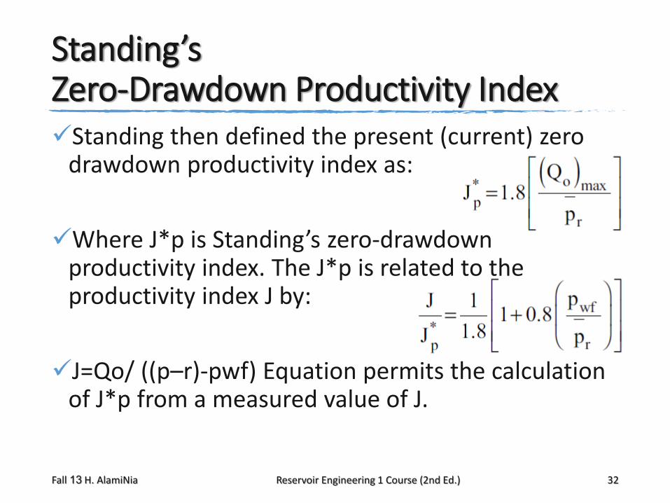
Standing’s Zero-Drawdown Productivity IndexStanding then defined the present (current) zero

drawdown productivity index as:

Where J*p is Standing’s zero-drawdown productivity index. The J*p is related to the productivity index J by:

J=Qo/ ((p–r)-pwf) Equation permits the calculation of J*p from a measured value of J.


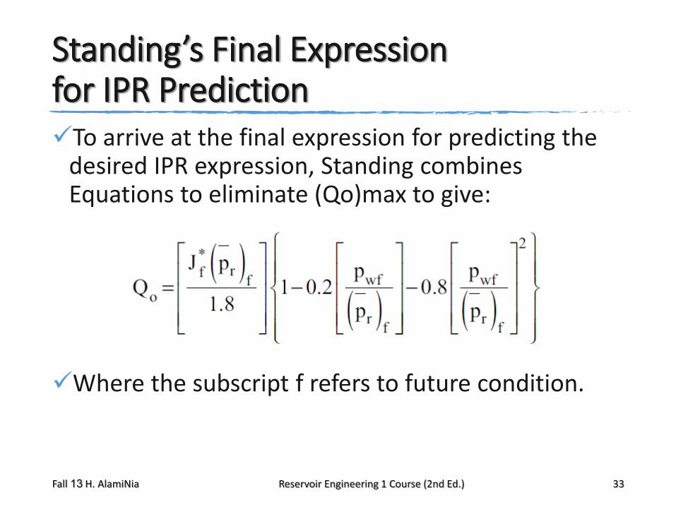
Standing’s Final Expression for IPR PredictionTo arrive at the final expression for predicting the

desired IPR expression, Standing combines Equations to eliminate (Qo)max to give:

Where the subscript f refers to future condition.


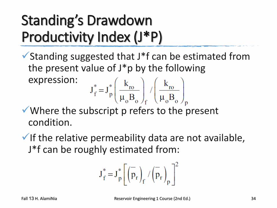
Standing’s Drawdown Productivity Index (J*P)Standing suggested that J*f can be estimated from

the present value of J*p by the following expression:

Where the subscript p refers to the present condition.

If the relative permeability data are not available, J*f can be roughly estimated from:


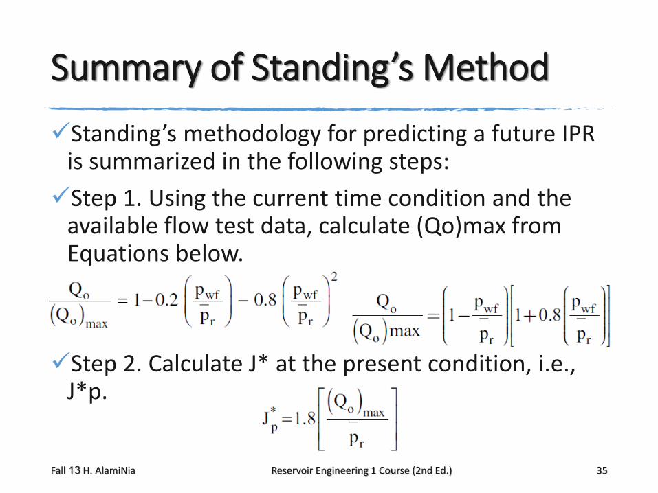
Summary of Standing’s Method

Standing’s methodology for predicting a future IPR is summarized in the following steps:

Step 1. Using the current time condition and the available flow test data, calculate (Qo)max from Equations below.

Step 2. Calculate J* at the present condition, i.e., J*p.


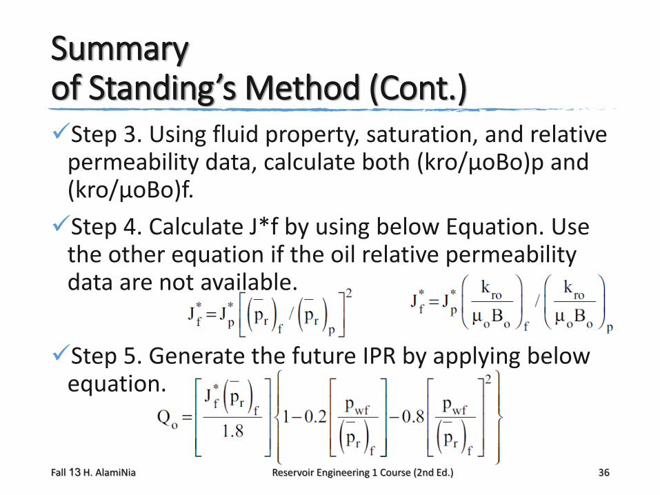
Summary of Standing’s Method (Cont.)Step 3. Using fluid property, saturation, and relative

permeability data, calculate both (kro/μoBo)p and (kro/μoBo)f.

Step 4. Calculate J*f by using below Equation. Use the other equation if the oil relative permeability data are not available.

Step 5. Generate the future IPR by applying below equation.


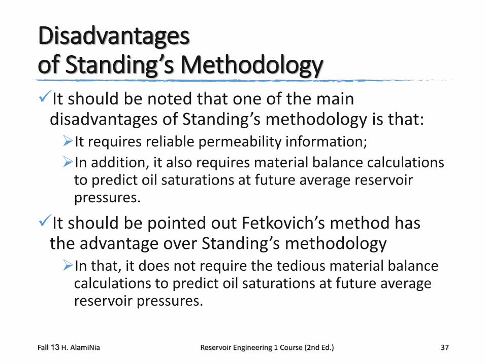
Disadvantages of Standing’s MethodologyIt should be noted that one of the main

disadvantages of Standing’s methodology is that:It requires reliable permeability information;

In addition, it also requires material balance calculations to predict oil saturations at future average reservoir pressures.

It should be pointed out Fetkovich’s method has the advantage over Standing’s methodology In that, it does not require the tedious material balance

calculations to predict oil saturations at future average reservoir pressures.


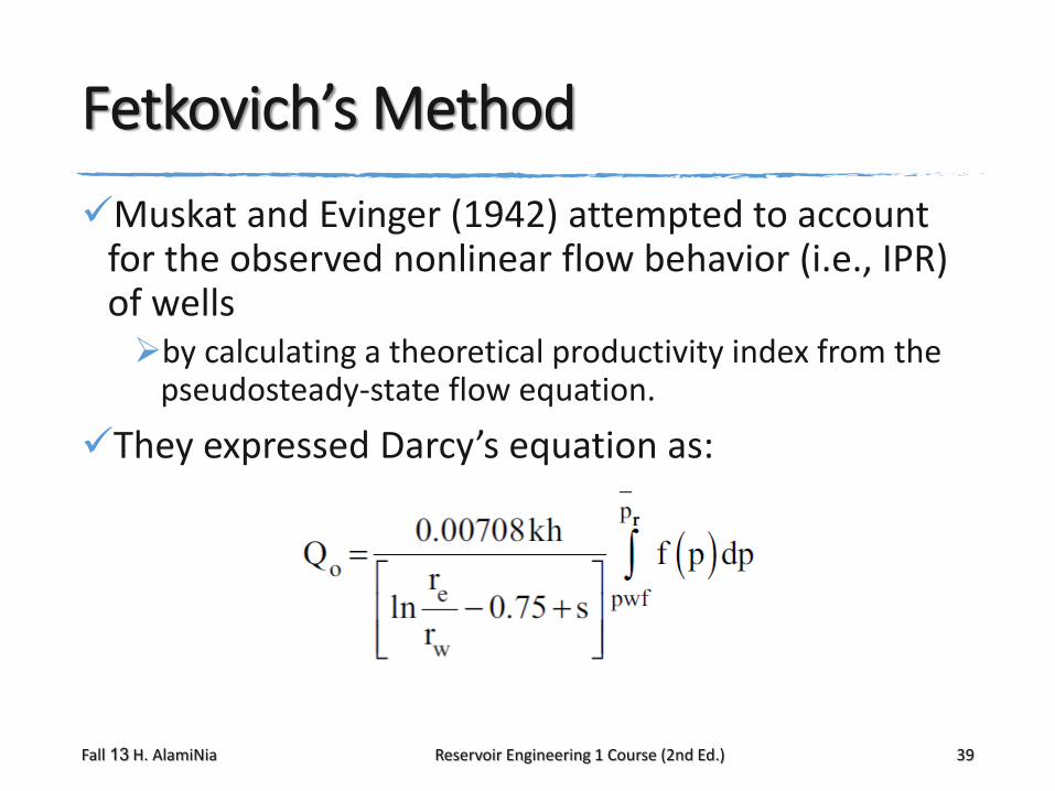
Fetkovich’s Method

Muskat and Evinger (1942) attempted to account for the observed nonlinear flow behavior (i.e., IPR) of wells by calculating a theoretical productivity index from the

pseudosteady-state flow equation.

They expressed Darcy’s equation as:


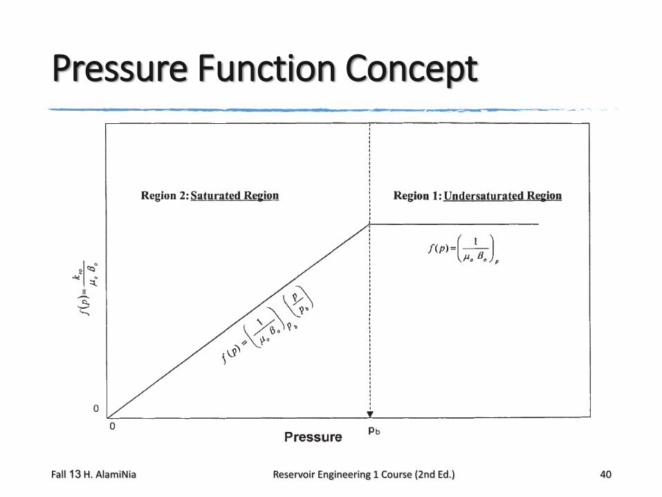
Pressure Function Concept


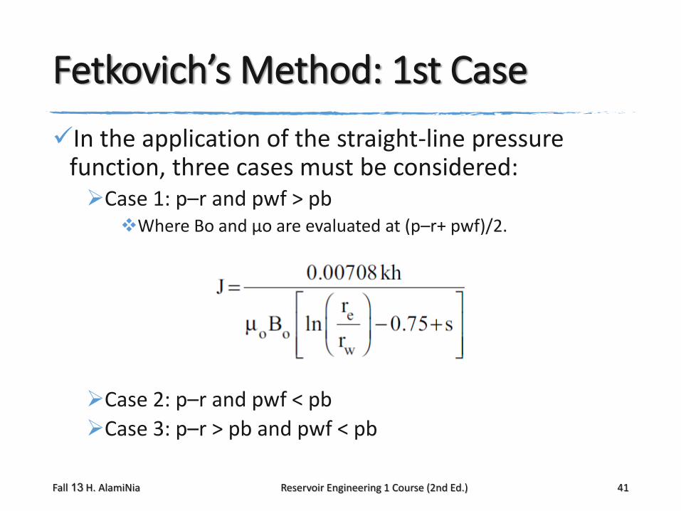
Fetkovich’s Method: 1st Case

In the application of the straight-line pressure function, three cases must be considered:Case 1: p–r and pwf > pb

Where Bo and μo are evaluated at (p–r+ pwf)/2.

Case 2: p–r and pwf < pb

Case 3: p–r > pb and pwf < pb


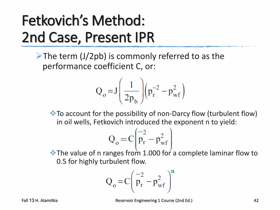
Fetkovich’s Method: 2nd Case, Present IPR

The term (J/2pb) is commonly referred to as the performance coefficient C, or:

To account for the possibility of non-Darcy flow (turbulent flow) in oil wells, Fetkovich introduced the exponent n to yield:

The value of n ranges from 1.000 for a complete laminar flow to 0.5 for highly turbulent flow.


Fetkovich’s Method: 2nd Case, Calculation of C and NThere are two unknowns in the Equation:

The performance coefficient C and the exponent n. At least two tests are required to evaluate these two

parameters:

A plot of p–2r− p2wf versus Qo on log-log scales will result in a straight line having a slope of 1/n and an intercept of C at p–2r− p2wf = 1.

The value of C can also be calculated using any point on the linear plot once n has been determined to give:


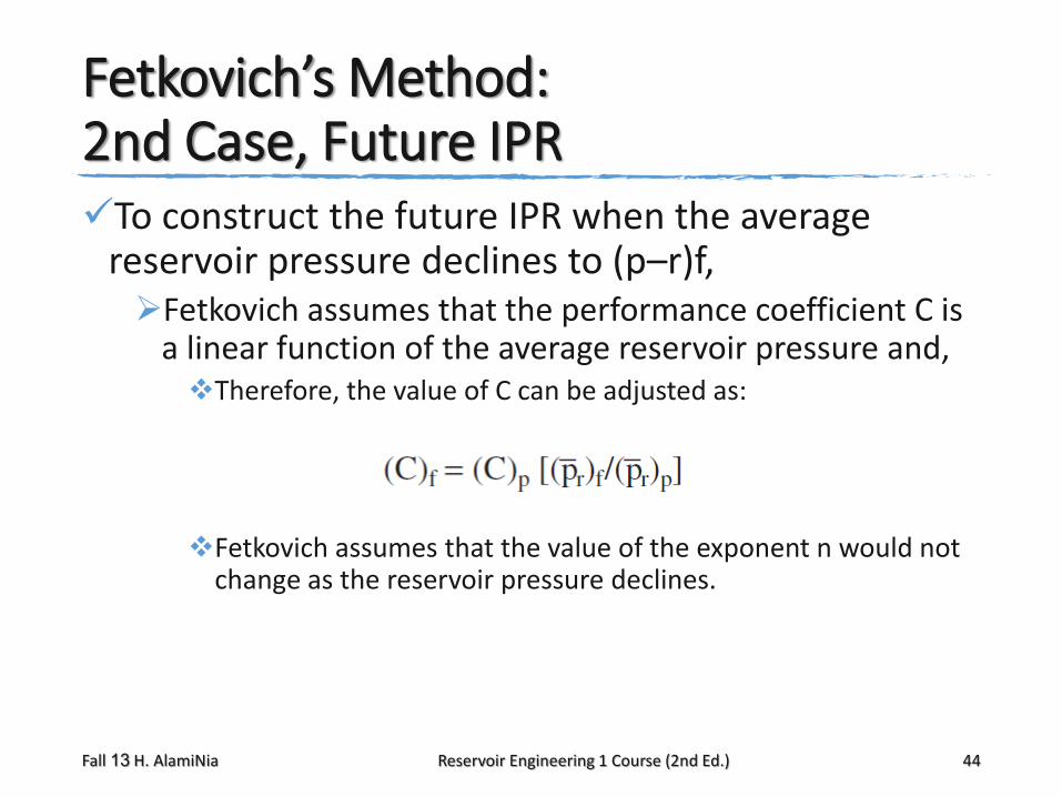
Fetkovich’s Method: 2nd Case, Future IPRTo construct the future IPR when the average

reservoir pressure declines to (p–r)f, Fetkovich assumes that the performance coefficient C is

a linear function of the average reservoir pressure and, Therefore, the value of C can be adjusted as:

Fetkovich assumes that the value of the exponent n would not change as the reservoir pressure declines.


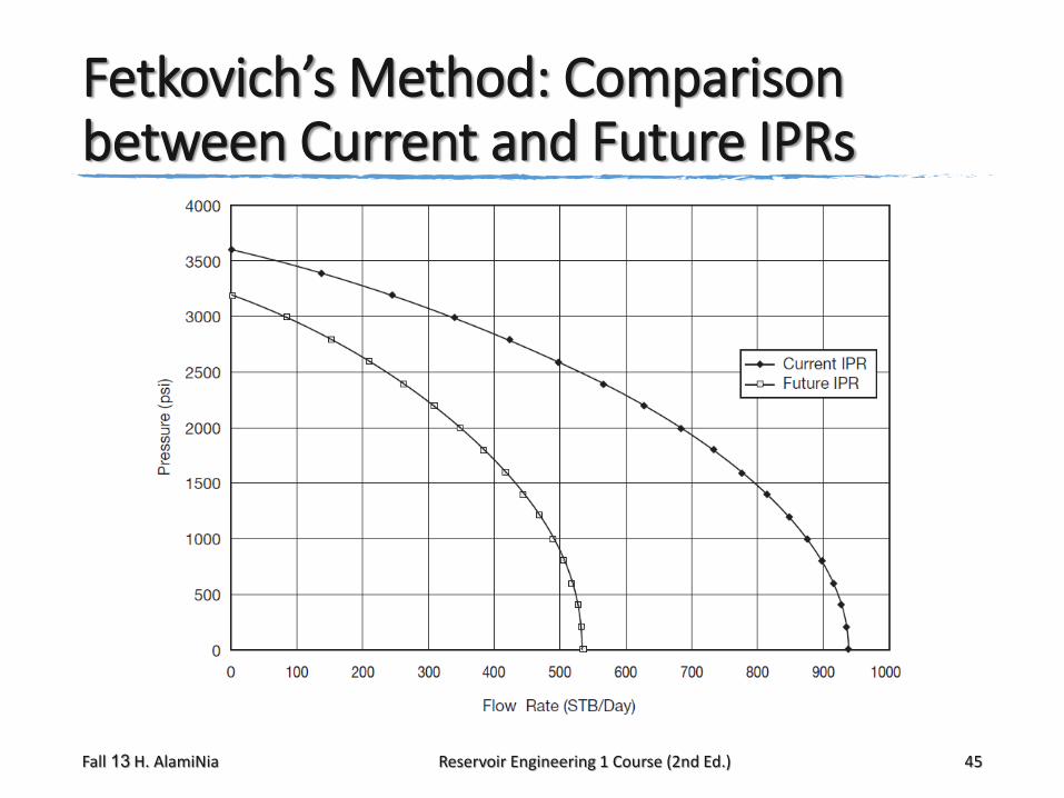
Fetkovich’s Method: Comparison between Current and Future IPRs


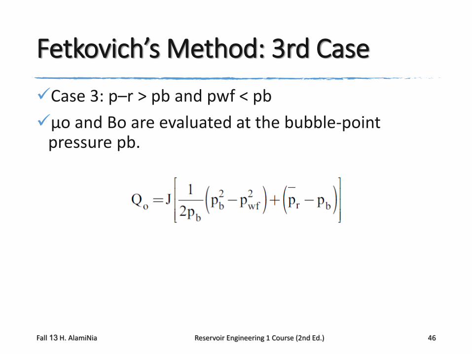
Fetkovich’s Method: 3rd Case

Case 3: p–r > pb and pwf < pb

μo and Bo are evaluated at the bubble-point pressure pb.


1. Ahmed, T. (2010). Reservoir engineering handbook (Gulf Professional Publishing). Chapter 7

1. Horizontal Oil Well Performance

2. Horizontal Well Productivity

3. Vertical Gas Well Performance

4. Pressure Application Regions

5. Turbulent Flow in Gas WellsA. Simplified Treatment Approach

B. Laminar-Inertial-Turbulent (LIT) Approach (Cases A. & B.)

Download - Q921 re1 lec11 v1

Top Related