Download - Probability, Statistics and Random Processes

ABDELKADER BENHARIABDELKADER BENHARIABDELKADER BENHARIABDELKADER BENHARI
PROBABILITY, STATISTICS AND RANDOM PROCESSESPROBABILITY, STATISTICS AND RANDOM PROCESSESPROBABILITY, STATISTICS AND RANDOM PROCESSESPROBABILITY, STATISTICS AND RANDOM PROCESSES
This course is an introduction to probability, statistics
and random processes

A.BENHARI -2-
Contents
I. POBABILITY .................................................................... 6
Basic Ideas of Probability ............................................................... 7
1. Probability Spaces ........................................................... 7
1.1. Discrete Probability Spaces ................................................... 8
1.2. Continuous Probability Spaces ................................................ 9
1.3. Properties of Probability ..................................................... 9
2. Conditional Probability and Statistical Independence ........................ 11
2.1. Conditional Probability ..................................................... 11
2.2. Composite Probability Formulae .............................................. 11
2.3. Bayes Formulae ........................................................... 12
2.4. Statistical Independence .................................................... 12
Appendix Combinatorics ......................................................... 13
Random Variables and Distributions ...................................................... 15
............................................................ 15 1. Random Variables
.................................................. 15 1.1. Discrete Random Variables
............................................... 18 1.2. Continuous Random Variables
................................. 21 1.3. Distributions of Functions of Random Variables
.......................... 23 2. Random Vectors (Multidimensional Random Variables)
................................................... 24 2.1. Discrete Random Vectors
................................................. 24 2.2. Continuous Random Vectors
................................... 24 2.3. Marginal Distributions/Probabilities/Densities
................................. 25 2.4. Conditional Distributions/Probabilities/Densities
........................................... 26 2.5. Independence of Random Variables
................................... 26 2.6. Distributions of Functions of Random VectorsMathematical Expectations (Statistical Average) of Random Variables ........................... 31
1. Mathematical Expectations (Statistical Average) ............................. 31
1.1. Definitions ............................................................... 31
1.2. Properties ................................................................ 32
1.3. Moments ................................................................ 32
1.4. Holder Inequality .......................................................... 34
2. Correlation Coefficients and Linear Regression (Approximation) .............. 35
3. Conditional Expectations and Regression Analysis ............................ 37
4. Generating and Characteristic Functions ..................................... 38
5. Normal Random Vectors ....................................................... 40
Memo ........................................................................... 42
Definition ................................................................... 42
Examples ................................................................... 42
Properties ................................................................... 42
Linear Regression ............................................................. 43
Regression .................................................................. 43
Normal Distribution ........................................................... 43
Limit Theorems ...................................................................... 44
A.BENHARI -3-
1. Inequalities ................................................................ 44
2. Convergences of Sequences of Random Variables ............................... 45
3. The Weak Laws of Large Numbers .............................................. 46
4. The Strong Laws of Large Numbers ............................................ 47
5. The Central Limit Theorems .................................................. 49
Conditioning. Conditioned distribution and expectation. ............................ 51
1. The conditioned probability and expectation. ................................ 51
2. Properties of the conditioned expectation. .................................. 53
3. Regular conditioned distribution of a random variable. ...................... 59
Transition Probabilities ........................................................... 67
1. Definitions and notations. .................................................. 67
2. The product between a probability and a transition probability. ............. 68
3. Contractivity properties of a transition probability. ....................... 70
4. The product between transition probabilities. ............................... 73
5. Invariant measures. Convergence to a stable matrix .......................... 74
Disintegration of the probabilities on product spaces .............................. 75
1. Regular conditioned distributions. Standard Borel Spaces .................... 75
2. The disintegration of a probability on a product of two spaces ............... 78
3. The disintegration of a probability on a product of n spaces ................. 79
The Normal Distribution ........................................................ 83
1. One-dimensional normal distribution .......................................... 83
2. Multidimensional normal distribution ........................................ 83
3. Properties of the normal distribution ........................................ 86
4. Conditioning inside normal distribution ...................................... 88
5. The multidimensional central limit theorem ................................... 91
II. STATISTCS ..................................................................... 95
Basic Concepts ....................................................................... 96
1. Populations, Samples and Statistics ......................................... 97
2. Sample Distributions ........................................................ 99
2.1. 2χ (Chi-Square)-Distribution ................................................ 99
2.2. t(Student)-Distribution .................................................... 100
2.3. F-Distribution ........................................................... 100
3. Normal Populations ......................................................... 103
Parameter Estimation ................................................................. 104
1. Point Estimation ........................................................... 105
1.1. Point Estimators ......................................................... 105
1.2. Method of Moments (MOM)................................................ 105
1.3. Maximum Likelihood Estimation (MLE) ...................................... 106
2. Interval Estimation ........................................................ 108
Tests of Hypotheses .................................................................. 111
1. Parameters from a Normal Population ........................................ 112
2. Parameters from two Independent Normal Populations ......................... 115
A.BENHARI -4-
III. RANDOM PTOCESSES ...................................................... 118
Introduction ........................................................................ 119
1. Definition ................................................................. 120
2. Family of Finite-Dimensional Distributions ................................. 121
3. Mathematical Expectations .................................................. 122
4. Examples ................................................................... 123
4.1. Processes with Independent, Stationary or Orthogonal Increments .................. 123
4.2. Normal Processes ........................................................ 124
Markov Processes (1) ................................................................. 125
1. General Properties ......................................................... 126
2. Discrete-Time Markov Chains ................................................ 128
2.1. Transition Probabilities .................................................... 128
2.2. Classification of States .................................................... 130
2.3. Stationary & Limit Distributions ............................................. 135
2.4. Examples: Simple Random Walks ........................................... 136
Appendix Eigenvalue Diagonalization ........................................... 138
Markov Processes (2) ................................................................. 140
1. Continuous-Time Markov Chains .............................................. 141
1.1. Transition Rates .......................................................... 141
1.2. Kolmogorov Forward and Backward Equations ................................. 142
1.3. Fokker-Planck Equations .................................................. 144
1.4. Ergodicity .............................................................. 145
1.5. Birth and Death Processes .................................................. 146
1.6. Poisson Processes ........................................................ 147
Appendix Queuing Theory .................................................... 153
2. Continuous-Time and Continuous-State Markov Processes ...................... 155
2.1. Basic Ideas .............................................................. 155
2.2. Wiener Processes ......................................................... 156
Hidden Markov Models ............................................................... 159
1. Definition of Hidden Markov Models ......................................... 160
2. Assumptions in the theory of HMMs .......................................... 161
3. Three basic problems of HMMs√ .............................................. 163
3.1. The Evaluation Problem ................................................... 163
3.2. The Decoding Problem .................................................... 163
3.3. The Learning Problem ..................................................... 163
4. The Forward/Backward Algorithm and its Application to the Evaluation Problem 165
5. Viterbi Algorithm and its Application to the Decoding Problem .............. 167
6. Baum-Welch Algorithm and its Application to the Learning Problem ........... 169
6.1. Maximum Likelihood (ML) Criterion ......................................... 169
6.2. Baum-Welch Algorithm ................................................... 169
Second-Order Processes and Random Analysis ............................................. 172
1. Second-Order Random Variables and Hilbert Spaces ........................... 173

A.BENHARI -5-
2. Second-Order Random Processes .............................................. 174
2.1. Orthogonal Increment Random Processes ...................................... 174
3. Random Analysis ............................................................ 176
3.1. Limits ................................................................. 176
3.2. Continuity .............................................................. 176
3.3. Derivatives ............................................................. 177
3.4. Integrals ................................................................ 178
Stationary Processes .................................................................. 179
1. Strictly Stationary Processes .............................................. 180
2. Weakly Stationary Processes ................................................ 181
2.1. Definition .............................................................. 181
2.2. Properties of Correlation/Covariance Functions ................................. 181
2.3. Periodicity .............................................................. 182
2.4. Random Analysis ........................................................ 182
2.5. Ergodicity (Statistical Average = Time Average) ................................ 183
2.6. Spectrum Analysis & White Noise ........................................... 184
3. Discrete Time Sequence Analysis: Auto-Regressive and Moving-Average (ARMA)
Models ........................................................................ 186
3.1. Definition .............................................................. 186
3.2. Transition Functions ...................................................... 186
3.3. Mathematical Expectations ................................................. 188
3.4. Parameter Estimation ..................................................... 189
4. Problems ................................................................... 193
Martingales ....................................................................... 196
1. Simple properties ..................................................... 197
2. Stopping times ........................................................ 199
3. An application: the ruin problem. ..................................... 205
Convergence of martingales ........................................................ 207
1. Maximal inequalities .................................................. 207
2. Almost sure convergence of semimartingales ............................ 210
3. Uniform integrability and the convergence of semimartingales in L
1
.... 214
4. Singular martingales. Exponential martingales. ........................ 218
Bibliography: ...................................................................... 221

A.BENHARI -6-
I. POBABILITY
A.BENHARI -7-
Basic Ideas of Probability
1. Probability Spaces
There are two definitions of probabilities for random events: classical and modern. The
modern definition of probability is based on the measure theory in which a random event is
nothing but a set and its probability is the measure of the set.
Definition (Sigma-Algebra) Let Ω be a set and Π a class Π of subsets of Ω , i.e., a subset
of Ω2 , Π is said to be a algebra−σ of Ω if
(1) Π∈Ω
(2) if Π∈A , then Π∈−Ω= AA (which implies that Π∈φ )
(3) if Π∈iA , where Ii ∈ and I is at most a countable index set, then Π∈∈U
IiiA (which
means that the class Π is closed with respect to union)
Remark 1: Ω2 is the power set of Ω , i.e., the set of all subsets of Ω .
Remark 2: In measure theory, ( )ΠΩ, is called a measurable space.
Remark 3: Since Π∈==∈∈∈UII
Iii
Iii
Iii AAA , Π is also closed with respect to intersection.
Example Let 21,ωω=Ω , 2121 ,,,, ωωωωφ=Π , where φ stands for empty set, Π is
then a ebralga−σ .
Definition (Probability Space) Let Ω be a set, Π a σ-algebra of Ω and P a real-valued
function defined on Π , the triplet ( )P,,ΠΩ is called a probability space if P satisfies the
following conditions
(1) ( ) 0AP ≥ for all Π∈A

A.BENHARI -8-
(2) ( )∑+∞
=
+∞
=
=
1ii
1ii APAP U for all Π∈LL ,A,,A,A n21 such that φ=ji AA I when
ji ≠
(3) ( ) 1P =Ω (which implies that ( ) 0P =φ )
Remark 1: Usually, Ω is often called sample space, Π the field of random events and for all
Π∈A , ( )AP the probability of occurrence of A.
Remark 2: In measure theory, the probability space ( )P,,ΠΩ is also called measured space.
Remark 3: Two random events A and B are said to be incompatible if φ=AB . In this case,
( ) 0ABP = .
1.1. Discrete Probability Spaces
The number of all possible occurrences in a random experiment is countable.
Definition A probability space ( )P,,ΠΩ is called a discrete probability space if the sample
space Ω is a countable (finite or denumerable infinite) set and Ω=Π 2 .
Remark 1: To specify a discrete probability P, it suffices to specify a mapping [ ]1,0:p →Ω
such that ( ) 0p ≥ω for all Ω∈ω and ( ) 1p =ω∑Ω∈ω
. Then, for all Π∈A , ( ) ( )∑∈ω
ω=A
pAP .
Remark 2: If N21 ,,, ωωω=Ω L and ( )N
1p i =ω , where N,,2,1i L= , then the resulting
triple ( )P,,ΠΩ is called classical probability space.
Example Let 21,ωω=Ω , 2121 ,,,, ωωωωφ=Π , and
(1) ( )3
1p 1 =ω , ( )
3
2p 2 =ω , then ( )P,,ΠΩ is a discrete probability space
(2) ( ) ( )2
1pp 21 =ω=ω , then ( )P,,ΠΩ is a classical probability space
A.BENHARI -9-
Example Let LL ,,,, n21 ωωω=Ω , Ω=Π 2 and ( )( )2
1k2
2
nn
6
k
1n
1
pπ
==ω∑
∞+
=
, L,2,1n = , then
( )P,,ΠΩ is a discrete probability space.
1.2. Continuous Probability Spaces
The number of all possible occurrences in a random experiment is uncountable.
Definition A probability space ( )P,,ΠΩ is called a continuous probability space if the
sample space Ω is a continuum.
Example (Geometric Probability) Assume that the sample Ω is an interval, an area or a
volume, then the probability of a point falling into a part of Ω is given by
ΩΩ
=ofMeasure
ofparttheofMeasureP
1.3. Properties of Probability
Theorem (Finite Measure) Let ( )P,,ΠΩ be a probability space, then for all Π∈A ,
( ) ( ) ( ) 1PAPAP =Ω=+ ⇒ ( ) 1AP ≤
Theorem (Monotonicity) Let ( )P,,ΠΩ be a probability space, then for all Π∈B,A ,
BA ⊆ ⇒ ( ) ( ) ( ) ( )BPABPAPAP =−+≤
Theorem (Union) Let ( )P,,ΠΩ be a probability space, then for all Π∈B,A ,
A.BENHARI -10-
( ) ( )( ) ( ) ( ) ( ) ( ) ( )BAPBPAPABPAPABAPBAP IUU −+=−+=−=
Theorem (Union) Let ( )P,,ΠΩ be a probability space, then for all Π∈n21 A,,A,A L ,
( ) ( )∑ ∑= ≤<<≤
−
=
−=
n
1k nii1ii
1kn
1ii
k1
k1AAP1AP
L
LU
Hint:
( ) ( )
−+
=
=++
=
+
=UUU
n
1i1ni1n
n
1ii
1n
1ii AAPAPAPAP
( ) ( ) ( ) ( ) ( )∑ ∑∑ ∑= ≤<<≤
+−
+= ≤<<≤
−
−−+
−=n
1k nii11nii
1k1n
n
1k nii1ii
1k
k1
k1
k1
k1AAAP1APAAP1
LL
LL
( ) ( )1nni1
i APAP1
1 +≤≤
+= ∑
( ) ( ) ( ) ( )∑ ∑∑ ∑−
= ≤<<≤+
= ≤<<≤
−
−+
−+1n
1k nii11nii
kn
2k nii1ii
1k
k1
k1
k1
k1AAAP1AAP1
LL
LL
( ) ( )∑≤<<≤
+−+nii1
1niin
n1
n1AAAP1
L
L
( )∑+≤≤
=1ni1
iAP
( ) ( ) ( )∑ ∑∑= ≤<<≤
+≤<<≤
−
+−+−
−
n
2k nii11nii
nii1ii
1k
1k1
1k1
k1
k1AAAPAAP1
LL
LL
( ) ( )1nn1n AAAP1 +−+ L
( )∑+≤≤
=1ni1
iAP ( ) ( )∑ ∑= +≤<<≤
−
−+n
2k 1nii1ii
1k
k1
k1AAP1
L
L ( ) ( )1nn1n AAAP1 +−+ L
( ) ( )∑ ∑+
= +≤<<≤
−
−=1n
1k 1nii1ii
1k
k1
k1AAP1
L
L
A.BENHARI -11-
2. Conditional Probability and Statistical Independence
2.1. Conditional Probability
Definition Let ( )P,,ΠΩ be a probability space and Π∈B,A , the conditional probability of
B, given that A has occurred, is defined as ( ) ( )( )AP
ABPABP = , where ( ) 0AP > .
Theorem Let ( )P,,ΠΩ be a probability space and Π∈A with ( ) 0AP > , the triplet
( )AAA P,,ΠΩ is also a probability space, where AA IΩ=Ω , Π∈=Π BABA and
( ) ( )ABPABPA = .
2.2. Composite Probability Formulae
Theorem (Composite Probability Formula) Let ( )P,,ΠΩ be a probability space, and
Π∈A , if Uk
kEA ⊆ , where Π∈kE with ( ) 0EP k > and φ=ji EE I for all ji ≠ , then
( ) ( ) ( )∑=k
kk EPEAPAP .
Proof:
( ) ( ) ( ) ( ) ( )∑∑ ==
=
=k
kkk
kk
kk
k EPEAPAEPAEPEAPAP UU #
Remark:
ABABA =⇒⊆ I , ( )UU IIk
kk
k EAEA =
A.BENHARI -12-
2.3. Bayes Formulae
Theorem (Bayes Formula) Let ( )P,,ΠΩ be a probability space and Π∈A with ( ) 0AP > ,
if Uk
kEA ⊆ , where Π∈kE with ( ) 0EP k > and φ=ji EE I for all ji ≠ , then
( ) ( ) ( )( ) ( )∑
=
kkk
iii EAPEP
EAPEPAEP .
Proof:
( ) ( )( )
( ) ( )( ) ( )∑
==
kkk
iiii EAPEP
EAPEP
AP
AEPAEP #
2.4. Statistical Independence
Definition Let ( )P,,ΠΩ be a probability space and Π∈B,A , A and B are said to be
statistically independent if ( ) ( ) ( )BPAPABP = .
Remark 1: If A and B are independent, then ( ) ( )( ) ( )APBP
ABPBAP == .
Remark 2: Recall that two events A and B are said to be incompatible if φ=AB . In this
case, ( ) 0ABP = .
Definition Let ( )P,,ΠΩ be a probability space and Π′ a subset of Π , Π′ is said to be
statistically independent if for all finite subsets Π ′′ of Π′ , ( )∏Π ′′∈Π ′′∈
=
AA
APAP I .
Remark: The statistical independence of any two events of Π′ can not guarantee the
statistical independence of Π′ . For example, C,B,A=Π′ , Π′ is statistically independent if
( ) ( ) ( )BPAPABP = , ( ) ( ) ( )CPAPACP = , ( ) ( ) ( )CPBPBCP = , ( ) ( ) ( ) ( )CPBPAPABCP =
are established at the same time.

A.BENHARI -13-
Appendix Combinatorics
Sample Selection Suppose there are m distinguishable elements, how many ways there are in
which one can select r elements from these m distinguishable elements?
Order
counts?
Repetitions are
allowed?
(With/Without
replacement)
The number of ways
to choose the samples Remarks
Yes Yes rm Permutation
Yes No ( )!rm
!m
− Permutation
No Yes ( )
( )!1m!r
!1rm
−−+
Combination
No No ( )!rm!r
!m
− Combination
Balls into Cells There are eight different ways in which n balls can be placed into k cells:
Distinguish the
balls?
Distinguish the
cells?
Can cells be
empty?
The number of ways to
place n balls into k cells
Yes Yes Yes nk
Yes Yes No k!
k
n
No Yes Yes ( )
( )!1k!n
!1nk
−−+
No Yes No ( )
( ) ( )!kn!1k
!1n
−−−

A.BENHARI -14-
Yes No Yes ∑=
k
1r r
n
Yes No No
k
n
No No Yes ( )∑=
k
1rr np
No No No ( )npk
where ( )∑=
−
−=
k
1r
nrk rr
k1
!k
1
k
n is the Stirling cycle number and ( )npk the number of
partition of the number n into exactly k integer pieces.
A.BENHARI -15-
Random Variables and Distributions
1. Random Variables
Let ( )P,,ΠΩ be a probability space, a random variable ξ is a function Definition
( )NumberesalReR:f →Ω such that for all Rx ∈ , ( ) ( ) Π∈<ωξΩ∈ωω= x,xE .
In terms of measure theory, a random variable is in fact a measurable function Remark 1:
over the measurable space ( )ΠΩ, .
In application, a random variable can be used to depict a random experiment and Remark 2:
( )xE can be used to depict a result of the experiment, i.e., a random event.
Let ( )P,,ΠΩ be a probability space and ξ a random variable, then the probability Definition
( ) ( ) x,PxF <ωξΩ∈ωω=
is called the distribution (function) of ξ .
Let ( )xF be the distribution of a random variable, then Theorem
(1) ( )xF is monotone increasing
(2) ( )xF is continuous from left
(3) ( ) 0xFlimx
=−∞→
, ( ) 1xFlimx
=+∞→
If the distribution ( )xF is defined as ( ) ( ) x,PxF ≤ωξΩ∈ωω= , then ( )xF is Remark 1:
continuous from right.
For all ba < , ( ) ( )aFbFbaP −=<ξ≤ . Remark 2:
1.1. Discrete Random Variables
A random variable is said to be a discrete random variable if its distribution Definition
function is not continuous.

A.BENHARI -16-
If ξ is a discrete random variable, then ( ) ∑<
=ξ=<ξ=xk
kPxPxF . Note that Remark:
( )xF is continuous from left. For all x, ( ) ( )xF0xFxP −+==ξ .
1.1.1. Bernoulli Distribution
Example (Bernoulli Distribution) A discrete random variable ξ is said to have 10 −
(Bernoulli) distribution if
==−=
==ξothers0
0kqp1
1kp
kP , where 0p > and 1qp =+
In the case, we have
( )
>≤<
≤==ξ=<ξ= ∑
< 1x1
1x0q
0x0
kPxPxFxk
Note that ( )xF is continuous from left.
1.1.2. Binomial Distribution
A discrete random variable ξ is said to have a binomial Example (Binomial Distribution)
distribution if
knknk qpCkP −==ξ , where 0p > , 1qp =+ , n,,1,0k L= , ( )!kn!k
!nCn
k −=
Remark 1: Note that ( ) ∑=
−=+n
0k
knknk
n baCba
Remark 2: If let k=ξ be an event that among the n independent random experiments only
k experiments are successful, then knknk qpCkP −==ξ .
If for all n, .Constnpn =λ= , then Theorem
( ) λ−−
+∞→
λ=− e!k
p1pClimk
knn
kn
nk
n
proof:
A.BENHARI -17-
Recall that tx
xe
x
t1lim =
+∞→
, we have
( ) λ−−−
−
+∞→
λ=
λ−
−−
−λ=
λ−
λ=− e!kn
1n
1k1
n
11
!kn1
nCp1pClim
kknkknknk
knn
kn
nk
nL #
For n large enough, ( ) ( ) npk
knknk e
!k
npp1pC −− ≈− Remark:
Example If the variables n21 ,,, ξξξ L are statistically independent and distributed with the
same 1~0 distribution, then the variable ∑=
ξ=ξn
1ii possesses the binomial distribution.
1.1.3. Negative Binomial Distribution
A discrete random variable ξ is said to have a Example (Negative Binomial Distribution)
negative binomial distribution if
nkn1k1n qpCkP −−
−==ξ , where 0p > , 1qp =+ and L,1n,nk +=
1.1.4. Geometric Distribution
A discrete random variable ξ is said to have a geometric Example (Geometric Distribution)
distribution if
pqkP 1k−==ξ , where 0p > , 1qp =+ and L,1,0k =
Remark: If let k=ξ be an event such that the kth experiment is first successful one, then
pqkP 1k−==ξ .
1.1.5. Hypergeometric Distribution
A discrete random variable ξ is said to have a Example (Hypergeometric Distribution)
hypergeometric distribution if
Nn
MNkn
Mk
C
CCkP
−−==ξ , where NM < , Mk ≤ , Nn ≤ and n,,1,0k L=
A.BENHARI -18-
1.1.6. Poission Distribution
A discrete random variable ξ is said to have a Poisson Example (Poission Distribution)
distribution if
λ−λ==ξ e!k
kPk
, where 0>λ , L,1,0k =
1.2. Continuous Random Variables
A random variable is said to be a continuous random variable if its distribution Definition
function is continuous.
A function ( )xf is called a probability density function if ( ) 0xf ≥ and Definition
( ) 1dxxf =∫+∞
∞−
.
It can be easily proven that the function Remark:
( ) ( )∫∞−
ττ=x
dfxF
is a distribution function, i.e., ( )xF is monotone increasing, continuous and ( ) 0xFlimx
=−∞→
,
( ) 1xFlimx
=+∞→
.
Let ξ be a continuous random variable with distribution ( )xF , then there must be a Theorem
probability density function ( )xf such that ( ) ( )∫∞−
ττ=x
dfxF .
Remark: For a continuous random variable, the relation between its distribution and its
probability density function is as follows:
( ) ( )∫∞−
ττ=x
dfxF ⇔ ( ) ( )xfxF =′
A.BENHARI -19-
1.2.1. Uniform Distribution
A continuous random variable ξ is said to have a uniform distribution if its Definition
density function is as follows:
( ) ( )
∈
−=others0
b,axab
1xf
1.2.2. Normal Distribution
A continuous random variable ξ is said to have a normal distribution ( )2,N σµ if Definition
its density function is as follows:
( )( )
2
2
2
x
e2
1xf σ
µ−−
σπ= , ( )+∞∞−∈ ,x
1.2.3. Exponential Distribution
A continuous random variable ξ is said to have an exponential distribution if its Definition
density function is as follows:
( )
<≥λ
=λ−
0x0
0xexf
x
, where 0>λ
The distribution of ξ follows immediately: Remark:
( ) ( )
<
≥−=λ==<ξ=λ−λ−
∞−
∫∫0x0
0xe1dtedttfxPxF
xx
0
tx
Theorem (Necessary Conditions) If a random variable ξ is exponentially distributed with
the parameter λ , then for all 0x ≥ and 0x >∆ , we have
( )xoxxxxP ∆+∆λ=≥ξ∆+<ξ
where ( )xo ∆ is the higher order infinitesimal of x∆ , i.e., ( )
0x
xolim
0x=
∆∆
→∆.
Proof:
(1) At first, we have
A.BENHARI -20-
( ) xPe
e
e
xP
xxP
xP
x;xxPxxxP x
x
xx
∆≥ξ===≥ξ
∆+≥ξ=≥ξ
≥ξ∆+≥ξ=≥ξ∆+≥ξ ∆λ−λ−
∆+λ−
This property is often called memoryless.
(2) From the memoryless property, we further have
xPxP1xxxP1xxxP ∆<ξ=∆≥ξ−=≥ξ∆+≥ξ−=≥ξ∆+<ξ
( ) ( )( ) ( ) ( )
( )xox!k
x1xe1
2k
kk
!k
x1xo2k
kkx ∆+∆λ=∆λ−+∆λ=−=
∑∆λ−=∆
+∞
=
∆λ−
∞+
=
∑ #
Remark: ∑+∞
=
=0n
nx
!n
xe .
Theorem (Sufficient Conditions) If a continuous random variable ξ satisfies the following
conditions
10P =≥ξ ; ( )xoxxxxP ∆+∆λ=≥ξ∆+<ξ for all 0x ≥ and 0x >∆
then it must be exponentially distributed with the parameter λ .
Proof:
Let ( ) tPtp ≥ξ= , then we have ( ) 10P0p =≥ξ= and
( ) tPtttPt;ttPttPttp ≥ξ≥ξ∆+≥ξ=≥ξ∆+≥ξ=∆+≥ξ=∆+
[ ] ( ) ( )[ ] ( )tptot1tptttP1 ∆+∆µ−=≥ξ∆+<ξ−=
which leads to
( ) ( ) ( ) ( ) ( ) ( )tptpt
tolim
t
tpttplimtp
0t0tµ−=
∆∆+µ−=
∆−∆+=′
→∆→∆ ⇒
( )µ−=
dt
tplnd
⇒ ( ) ( ) tt ee0ptp µ−µ− == ⇒ ( ) ( ) te1tp1tP1tPtF µ−−=−=≥ξ−=<ξ=
This shows that the random variable ξ is exponentially distributed. #
Example (Speaking Time) Suppose the probability of a telephone being used at time t and
released during the coming period ( ]tt,t ∆+ is ( )tot ∆+∆µ , what’s the distribution of time T
during which the telephone is being used, i.e., the speaking time of a telephone user?
A.BENHARI -21-
Example Suppose there are n persons speaking at time t, what’s the probability of the event
that 2 or more persons finish speaking in the coming time period ( ]tt,t ∆+ ?
Solution:
Let iξ be a random variable such that 1i =ξ represents the event that the ith person finishes
speaking in the time period ( ]tt,t ∆+ , then
( )tot1p i ∆+∆λ==ξ , ( )tot10p i ∆+∆λ−==ξ
where n,,2,1i L= . Thus, the random variable ∑=
ξn
1ii represents the number of persons who
finish speaking in the coming time period, which leads to
t
1P0P1
limt
2P
lim
n
1ii
n
1ii
0t
n
1ii
0t ∆
=ξ−
=ξ−
=∆
≥ξ ∑∑∑
==
→∆
=
→∆ ++
( )[ ] ( )[ ] ( )[ ]0
t
tot1totntot11lim
1nn
0t=
∆∆+∆λ−∆+∆λ−∆+∆λ−−=
−
→∆ +
This means that ( )to2Pn
1ii ∆=
≥ξ∑
=. #
1.2.4. Gamma Distribution
A continuous random variable ξ is said to have a Gamma distribution if its Definition
density function is as follows:
( ) ( )
≤
>γΓ
λ=
λ−−γγ
0x0
0xexxf
x1
, where 0>λ , 0>γ
Gamma Function: ( ) ∫+∞
−−γ=γΓ0
t1 dtet , where 0>γ . Remark:
1.3. Distributions of Functions of Random Variables
Given the distribution of ξ , what is the distribution of ( )ξg ?
Let ξ be a random variable, ( )xg a continuous function and ( )ξ=η g , Example
A.BENHARI -22-
If the function ( )xg is strictly monotone-increasing, then
( ) ( ) ( )( )
( )( )
∫∫−
∞−ξ
<ξη ==<ξ=η=
yg
yxg
1
dxxfdxxfygPyF ⇒ ( ) ( ) ( )( ) ( )dy
ydgygf
dy
ydFyf
11
−−
ξη
η ==
If the function ( )xg is strictly monotone-decreasing, then
( ) ( ) ( )( )
( )( )∫∫
+∞
ξ<
ξη−
==<ξ=η=ygyxg 1
dxxfdxxfygPyF ⇒ ( ) ( ) ( )( ) ( )dy
ydgygf
dy
ydFyf
11
−−
ξη
η −==
To sump up, when ( )xg is continuous and strictly monotone, Remark 1:
( ) ( ) ( )( ) ( )dy
ydgygfyf
11
g
−−
ξξ=η =
( )( )
( )( ) ( )( ) ( ) ( )( ) ( )
( )
( )
∫∫ ∂∂+′−′=
xg
xf
xg
xf
dtx
t,xhxf,xhxfxg,xhxgdtt,xh
dx
d Remark 2:
Let ξ be a random variable and ba += ξη , 0>a , then Example (Linear Transform)
( )
−=
−
<=<+==a
byF
a
byPybaPyF ξη ξξη
⇒ ( ) ( )
−=
−
==a
byf
adya
bydF
dy
ydFyf ξ
ξη
η1
For 0≠a , ( )
−=a
byf
ayf ξη
1. Remark:
Let ξ be a random variable and 2ξη = , then Example (Parabolic Function)
( ) ( ) ( )
≤>−−=<<−=<==
00
02
y
yyFyFyyPyPyF ξξ
ηξξη
⇒ ( ) ( ) ( ) ( )
≤
>−+
==00
02
y
yy
yfyf
dy
ydFyf
ξξη
η
A.BENHARI -23-
Let ξ be a random variable and ξ=η e , then Example (Exponential Function)
( ) ( )
≤>=<
=<==00
0lnln
y
yyFyPyePyF ξξ
ηξ
η
⇒ ( ) ( ) ( )
≤
>==00
0ln1
y
yyfy
dy
ydFyf ξη
η
Let ξ be a random variable and ξ=η ln , then Example (Logarithmic Function)
( ) ( ) ( )ye
0
eFdxxfylnPyF
y
ξξη ==<ξ=η= ∫ ⇒ ( ) ( ) ( ) yy eefdy
ydFyf ξ
ηη ==
Let ξ be a random variable and ξ=η sin , then Example (Triangular Function)
( ) ( )( )
−≤
≤<−
>
=<== ∑ ∫∞+
−∞=
−−
+
−
−
10
11
11
sin
1
1
sin12
sin2
y
ydxxf
y
yPyFk
yk
yk
π
πξη ξη
2. Random Vectors (Multidimensional Random Variables)
Let n21 ,,, ξξξ L be n random variables defined on the same probability space, Definition
then the vector ( )n21 ,,, ξξξ L is called a random vector.
Let ( )nξξξ ,,, 21 L be a random vector, then for all ( ) nn Rxxx ∈,,, 21 L , the Definition
function
( ) nnn xxxPxxxF <<<= ξξξ ;;;,,, 221121 LL
is called the joint distribution function of ( )nξξξ ,,, 21 L .
Let ( )ηξ, be a random vector and ( )y,xF its joint distribution, then Example
A.BENHARI -24-
( ) ( ) ( ) ( )c,aFc,bFd,aFd,bFdc;baP +−−=<η≤<ξ≤
2.1. Discrete Random Vectors
If each component of a random vector ( )n21 ,,, ξξξ L is a discrete random Definition
variable, the random vector ( )n21 ,,, ξξξ L is then called a discrete random vector.
: If ( )n21 ,,, ξξξ L is a discrete random vector, then Remark
( ) =<ξ<ξ<ξ= nn2211n21 x;;x;xPx,,x,xF LL
∑ ∑ ∑< < <
=ξ=ξ=ξ=11 22 nnxk xk xk
nn2211 k;;k;kP LL
2.2. Continuous Random Vectors
If each component of a random vector ( )n21 ,,, ξξξ L is a continuous random Definition
variable, the random vector ( )n21 ,,, ξξξ L is then called a continuous random vector.
Let ( )n21 ,,, ξξξ L be a continuous random vector and ( )n21 x,,x,xF L its joint Theorem
distribution function, then there is a function with n variables ( )n21 x,,x,xf L such that
(1) ( ) 0x,,x,xf n21 ≥L
(2) ( ) 1dxdxdxx,,x,xf n21n21 =∫ ∫ ∫+∞
∞−
+∞
∞−
+∞
∞−
LLL
(3) ( ) ( )∫ ∫ ∫∞− ∞− ∞−
ττττττ=1 2 nx x x
n21n21n21 ddd,,,fx,,x,xF LLLL
: The function ( )n21 x,,x,xf L is called joint density function of ( )n21 ,,, ξξξ L , Remark
which characterizes the random vector completely.
2.3. Marginal Distributions/Probabilities/Densities
Let ( )n21 ,,, ξξξ L be a random vector and ( )n21 x,,x,xF L its distribution, then Definition
the marginal distribution of any sub-vector of ( )n21 ,,, ξξξ L , say, ( )p21 ,,, ξξξ L , np < , is
given by
A.BENHARI -25-
( ) ( )+∞=+∞== + n1pp21p21 x,,x,x,,x,xFx,,x,xF LLL
: In the discrete case, we prefer the marginal probability as followed: Remark
∑ ∑+
=ξ=ξ=ξ=ξ==ξ=ξ ++1p nk k
nn1p1ppp11pp11 k;;k;k;;kPk;;kP LLLL
In the continuous case, we prefer the marginal density as followed:
( ) ( )∫ ∫+∞
∞−
+∞
∞−++ ττττττ=τττ n1pn1pp1p21 dd,,,,,f,,,f LLLLL
2.4. Conditional Distributions/Probabilities/Densities
Let ( )nξξξ ,,, 21 L be a discrete random vector and ( )nxxxF ,,, 21 L its Definition
distribution, then the conditional distribution of ( )nξξξ ,,, 21 L , given that its sub-vector
( )np ξξ ,,1 L+ , np < , has taken a certain value, say, ( )np kk ,,1 L+ , is given by
( )
nnpp
xk xknnpppp
npp kkP
kkkkP
kkxxxF pp
npp ==
=====
++
< <++
+
∑ ∑+ ξξ
ξξξξ
ξξξξ ;;
;;;;;
,,,,,11
1111
121,,,,11
11 L
LLL
LLLL
Again, in the discrete case, we prefer the conditional probability to the conditional Remark:
distribution:
nn1p1p
nn1p1ppp11nn1p1ppp11 k;;kP
k;;k;k;;kPk;;kk;;kP
=ξ=ξ=ξ=ξ=ξ=ξ
==ξ=ξ=ξ=ξ++
++++
L
LLLL
Let ( )n21 ,,, ξξξ L be a continuous random vector and ( )n21 x,,x,xF L its Definition
distribution, then the conditional distribution of ( )n21 ,,, ξξξ L , given that the sub-vector
( )n1p ,, ξξ + L , np < , has taken certain values, say, ( )n1p x,,x L+ , is given by
( ) ( )( )∫ ∫
∞− ∞− +ξξ
++ξξξξ ττ
ττ=
+
+
1 p
n1p
n1pp1
x x
p1n1p
n1pp1n1pp21,,,, dd
x,,xf
x,,x,,,fx,,xx,,x,xF L
L
LLLLL
L
LL
In practice, the conditional density Remark:
( ) ( )( )n1p
n1pp1n1pp1 x,,xf
x,,x,,,fx,,x,,f
n1pL
LLLL
L +ξξ
++
+
ττ=ττ is preferred to the condition distribution.

A.BENHARI -26-
2.5. Independence of Random Variables
TDefinition n21 ,,, ξξξ L are said to be independent if for all he random variables
Rx,,x,x n21 ∈L ,
nn2211nn2211 xPxPxPx;;x;xP <ξ<ξ<ξ=<ξ<ξ<ξ LL
or expressed in distribution
( ) ( ) ( ) ( )n21n21 xFxFxFx,,x,xFn21n21 ξξξξξξ = LLL
Remark 1: n21 ,,, ξξξ L any subset of If the random variables are independent, then
n21 ,,, ξξξ L , say, k21 iii ,,, ξξξ L , nk < , is also independent, i.e.,
kk2211kk2211 iiiiiiiiiiii xPxPxPx;;x;xP <ξ<ξ<ξ=<ξ<ξ<ξ LL
: For discrete random variables, the independence can be stated as Remark 2
nn2211nn2211 xPxPxPx;;x;xP =ξ=ξ=ξ==ξ=ξ=ξ LL
Also, for continuous random variables, the independence can be stated as
( ) ( ) ( ) ( )n21n21 xfxfxfx,,x,xfn21 ξξξ= LL
where ( )n21 x,,x,xf L is the joint probability density function of n21 ,,, ξξξ L , and ( )xfiξ is
the probability density function of iξ , n,,2,1i L= .
2.6. Distributions of Functions of Random Vectors
Let ξ and η be two random variables and η+ξ=ζ , then Example (Addition)
( ) ( ) ( )∫ ∫∫∫+∞
∞−
−
∞−ξη
<+ξηζ
==<η+ξ=ζ= dydxy,xfdxdyy,xfzPzF
yz
zyx
( ) ( ) ( )∫∫ ∫∫ ∫∞−
ζ∞−
+∞
∞−ξη
+∞
∞− ∞−ξη=+
=
−=
−=
zzz
uyxduufdudyy,yufdyduy,yuf
where ( ) ( ) ( )∫+∞
∞−ξη
ζζ −== dyy,yzf
dz
zdFzf .
If the random variables ξ and η are independent, then
( ) ( ) ( ) ( ) ( )( )zf*fdyyfyzfdyy,yzfzf ηξ
+∞
∞−ηξ
+∞
∞−ξηζ =−=−= ∫∫

A.BENHARI -27-
Example (Addition) Let LL ,T,,T,T n21 be independent exponential random variables with
the same parameter µ . Show that the distribution of n21n TTTS +++= L is the gamma
distribution:
( ) ( )
<
≥−
µ=
µ−−
0x0
0xe!1n
xxf
x1nn
Sn, where 1n ≥
Solution:
When 1n = , the theorem is self-evident. For 1n ≥ , ∑=
=n
1kkn TS is first assumed to be gamma-
distributed, the distribution of 1nn1n TSS ++ += will be then given by
( ) ( ) ( ) ( )( )
( )x
n1nx
0
1nx1nx
0
txt1nn
TSS e!n
xdtte
!1ndtee
!1n
tdttxftfxf
1nn1n
µ−+
−µ−+
−−µ−−+∞
∞−
µ=−
µ=µ−
µ=−= ∫∫∫ ++
By induction, the theorem is workable. #
Remark: It follows that
( )( )
≥
=µ=
−µ=
−µ
=< µ−
−
→
µ−−
→→ +++
∫
2n0
1ne
!1n
xlim
x
dte!1n
t
limx
xSPlim x
1nn
0x
x
0
t1nn
0x
n
0x
⇒ ( )xoxSP n =< , 2n ≥
This remark shows that the probability of 2 or more telephones being called by a person
during a period is the higher order infinitesimal of the period.
Let ξ and η be two random variables, then Example (Subtraction)
( ) ( ) ( )∫ ∫∫∫+∞
∞−
+
∞−ξη
<−ξηζ
==<η−ξ=ζ= dydxy,xfdxdyy,xfzPzF
yz
zyx
( ) ( ) ( )∫∫ ∫∫ ∫∞−
ζ∞−
+∞
∞−ξη
+∞
∞− ∞−ξη=−
=
+=
+=
zzz
uyxduufdudyy,yufdyduy,yuf
where ( ) ( ) ( )∫+∞
∞−ξη
ζζ +== dyy,yzf
dz
zdFzf .
If the random variables ξ and η are independent, then
A.BENHARI -28-
( ) ( ) ( ) ( )∫∫+∞
∞−ηξ
+∞
∞−ξηζ +=+= dyyfyzfdyy,yzfzf
Let ξ and η be two random variables, then Example (Division)
( ) ( ) ( ) ( )∫ ∫∫ ∫∫∫∞−
+∞
ξη
+∞
∞−ξη
<
ξηζ
+
==
<ηξ=ζ=
0
zy0
zy
zy
x
dydxy,xfdydxy,xfdxdyy,xfzPzF
( ) ( )∫ ∫∫ ∫∞−
−∞
ξη
+∞
∞−ξη
=
+
=
0
z0
z
uy
xdyduy,uyyfdyduy,uyyf
( ) ( )∫ ∫∫∞− ∞−
ξη
+∞
ξη
−=
z 0
0
dudyy,uyyfdyy,uyyf
( ) ( )∫∫ ∫∞−
ζ∞−
+∞
∞−ξη =
=
zz
duufdudyy,uyfy
where ( ) ( ) ( )∫+∞
∞−ξη
ζζ == dyy,zyfy
dz
zdFzf .
Let ξ and η be two random variables, then Example (Multiplication)
( ) ( ) ( ) ( )∫ ∫∫ ∫∫∫∞−
∞+
ξη
∞+
∞−ξη
<ξηζ
+
==<ξη=ζ=
0
yz0
yz
zxy
dydxy,xfdydxy,xfdxdyy,xfzPzF
∫ ∫∫ ∫∞−
−∞
ξη
+∞
∞−ξη=
+
=
0
z0
z
uxydyduy,
y
uf
y
1dyduy,
y
uf
y
1
∫ ∫∫∞− ∞−
ξη
+∞
ξη
−
=
z 0
0
dudyy,y
uf
y
1dyy,
y
uf
y
1
( )∫∫ ∫∞−
ζ∞−
+∞
∞−ξη =
=
zz
duufdudyy,y
uf
y
1
where ( ) ( )∫
+∞
∞−ξη
ζζ
== dyy,
y
zf
y
1
dz
zdFzf .

A.BENHARI -29-
Suppose ξ and η are independent random variables with the same exponential Example
distribution λ , i.e.,
( ) ( ) ( )( )
>>λ
==+λ−
ηξξηothers0
0y,0xeyfxfy,xf
yx2
then
( )( )
>>=
<
ηξ=ϕ<η+ξ=ψ=
∫∫<<<+<
ξη
ψϕ
others0
0v,0udxdyy,xfv;uPv,uF v
y
x0,uyx0
( )
>>
+
++= ∫∫<<<<
ξη
=+=others0
0v,0udpdq1q
p
1q
p,
1q
pqf
vq0,up02
y
xq,yxp
⇒ ( ) ( ) ( )
>>
+λ=
+
++=λ−
ξηψϕ
others0
0v,0ue1v
u
1v
u
1v
u,
1v
uvf
v,ufu
2
2
2
Remark 1:
( )
( )
+−
+
++=
∂∂
∂∂
∂∂
∂∂
=+
=+
=2
2
q1
py,
q1
pqx
q1
p
q1
1q1
p
q1
q
q
y
p
yq
x
p
x
J ⇒ ( )dpdq
q1
pdpdqJdxdy
2+==
( )v,uf ψϕ can be obtained in another way: Remark 2:
( ) ( ) ∫ ∫∫∫+
λ−−
λ−
<<<<<+<
ξηψϕ λ
λ==
<
ηξ=ϕ<η+ξ=ψ=
v1
uv
0
xxu
vx
y
v0,u0v
y
x0,uyx0
dxedyedxdyy,xfv;uPv,uF
( )∫∫+
λ−+λ−+
λ−−λ−λ−
−λ=λ
−=
v1
uv
0
ux
v
v1v1
uv
0
xxuv
x
dxeedxeee
( ) ( )uuuu uee1v1
ve
v1
uve1
v1
v λ−λ−λ−λ− λ−−+
=+
λ−−+
=
⇒ ( ) ( )( )
<<
+λ
=∂∂
∂=
λ−ψϕ
ψϕ
others0
v0,u0e1v
u
vu
v,uFv,uf
u2
22
(Jacobian Transform) Let Theorem

A.BENHARI -30-
( )( )
( )
ξξξ
ξξξξξξ
=
η
ηη
n21n
n212
n211
n
2
1
,,,f
,,,f
,,,f
L
M
L
L
M →← −− encecorrespendonetoone
( )( )
( )
ηηη
ηηηηηη
=
ξ
ξξ
n21n
n212
n211
n
2
1
,,,g
,,,g
,,,g
L
M
L
L
M
then
( ) nn2211n21 y;;y;yPy,,y,yFn21
<η<η<η=ηηη LLL
( )( )( )
( )
∫
<
<<
ξξξ=
nn21n
2n212
1n211
n21
yx,,x,xf
yx,,x,xf
yx,,x,xfn21n21 dxdxdxx,,x,xf
L
M
L
L
L LL
( )( )
( )
( ) ( )[ ]∫
<
<<
ξξξ
=
==
=
nn
22
11
n21
n21nn
n2122
n2111
yu
yu
yun21n21nn211
x,,x,xfu
x,,x,xfu
x,,x,xfudududuJu,,u,ug,,u,,u,ugf
M
L
L
M
L
LLLLL
which leads to
( ) ( ) ( )[ ]Ju,,u,ug,,u,,u,ugfu,,u,uf n21nn211n21 n21n21LLLL LL ξξξηηη =
where
∂∂
∂∂
∂∂
∂∂
∂∂
∂∂
∂∂
∂∂
∂∂
=
n
n
2
n
1
n
n
2
2
2
1
2
n
1
2
1
1
1
u
g
u
g
u
g
u
g
u
g
u
gu
g
u
g
u
g
J
L
MOMM
L
L
is Jacobian matrix.

A.BENHARI -31-
Mathematical Expectations (Statistical Average) of
Random Variables
1. Mathematical Expectations (Statistical Average)
1.1. Definitions
Definition Let ξ be a discrete random variable and ( )xg a function, then the mathematical
expectation of ( )ξg is defined as
( )[ ] ( ) ∑ α=ξα=ξk
kk PggE
if ( ) +∞<α=ξα∑k
kk Pg .
Remark 1: If ( ) +∞<α=ξα∑k
kk Pg , ( )[ ]ξgE is then said to be well defined.
Remark 2: The definition can be easily generalized to multivariate distributions. For
example,
( )[ ] ( ) ∑ β=ηα=ξβα=ηξj,i
jiji ;P,g,gE
Definition Let ξ be a continuous random variable and ( )xg a function, then the
mathematical expectation of ( )ξg is defined as
( )[ ] ( ) ( )∫+∞
∞−
=ξ dxxfxggE
if ( ) ( ) +∞<∫+∞
∞−
dxxfxg , where ( )xf is the density function of ξ .
Remark 1: If ( ) ( ) +∞<∫+∞
∞−
dxxfxg , ( )[ ]ξgE is then said to be well defined.
Remark 2: The definition can be easily generalized to multivariate distributions. For
example,
A.BENHARI -32-
( )[ ] ( ) ( )∫ ∫+∞
∞−
+∞
∞−ξη=ηξ dxdyy,xfy,xg,gE
where ( )y,xf ξη is the joint density function of ξ and η.
1.2. Properties
Theorem The expectation [ ]•E is a linear operator, i.e.,
( ) ( )[ ] ( )[ ] ( )[ ]η+ξ=η+ξ gbEfaEgbfaE
where ( )xf and ( )xg are two functions, ξ and η two random variables and a and b two
numbers.
Theorem If two random variables ξ and η are independent, then
( ) ( )[ ] ( )[ ] ( )[ ]ηξ=ηξ gEfEgfE
where ( )xf and ( )xg are two functions.
Theorem Let ξ and η be two random variables, then
[ ] 0E2 =η−ξ ⇔ 1P =η=ξ
Remark: In terms of probability, 1P =η=ξ means η=ξ .
1.3. Moments
Definition Let ξ be a random variable, then
• [ ]kE ξ is called the k-th original moment of ξ if [ ]kE ξ is well defined.
• ( )[ ]kEE ξ−ξ is called the k-th central moment of ξ if ( )[ ]kEE ξ−ξ is well defined.
Remark 1: A random variable ξ is said to be second-order if [ ]2E ξ is well defined.
Remark 2: The first-order original moment of ξ is called the mean of ξ . The second-order
central moment of ξ is called the variance of ξ , often denoted by ξD .

A.BENHARI -33-
Example Let ξ be a second-order random variable and ξξ−ξ=η
D
E, then
[ ] 0E =η , [ ] 1D =η
Remark: The variable ξξ−ξ=η
D
E is often called the standardized/normalized variable of ξ .
Theorem (Variational Inequality) For all numbers α , ( )[ ] ( )[ ]22 EEE α−ξ≤ξ−ξ .
Hint: ( )[ ] ( )[ ] ( )[ ] ( ) ( )[ ]22222 EEEEEEE α−ξ≤ξ−α−α−ξ=ξ−α+α−ξ=ξ−ξ
Theorem If n21 ,,, ξξξ L are independent, then
( )
ξ−ξα=
ξα−ξα=
ξα ∑∑∑∑====
2n
1iiii
2n
1iii
n
1iii
n
1iii EEEED
( )( )[ ] ( )[ ] ∑∑∑∑=== =
ξα=ξ−ξα=ξ−ξξ−ξαα=n
1ii
2i
n
1i
2ii
2i
n
1i
n
1jjjiiji DEEEEE
Example
Bernoulli’s distribution:
=−
===ξ
0kp1
1kpkP , then
pE =ξ , ( )[ ] ( )p1pEED 2 −=ξ−ξ=ξ
Binormial distribution: knknk qpCkP −==ξ , n,,1,0k L= , then
npE =ξ , ( )[ ] npqEED 2 =ξ−ξ=ξ
Poisson distribution: λ−λ==ξ e!k
kP , L,2,1,0k = , then
λ=ξE , ( )[ ] [ ] ( ) λ=ξ−ξ=ξ−ξ=ξ 222 EEEED
Uniform distribution: ( ) ( )
∈
−=others0
b,axab
1xf , then
2
baE
+=ξ , ( )[ ] ( )12
abEED
22 −=ξ−ξ=ξ
A.BENHARI -34-
Exponential distribution: ( ) >λ
=λ−
others0
0xexf
x
, then
λ=ξ 1
E , ( )[ ]2
2 1EED
λ=ξ−ξ=ξ
Normal distribution: ( )( )
2
2
2
x
e2
1xf σ
µ−−
σπ= , ( )+∞∞−∈ ,x , then
µ=ξE , 2D σ=ξ
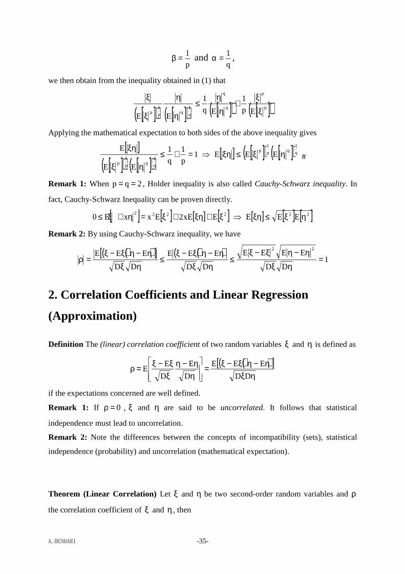
1.4. Holder Inequality
Theorem Suppose ξ and η are two random variables defined on the same probability space,
then
[ ] [ ]( ) [ ]( )q
1qp
1p
EEE ηξ≤ξη
where 1p > and 1q
1
p
1 =+ .
Proof:
(1) We first prove that vuvu β+α≤βα , where 0u ≥ , 0v ≥ , 10 <α< and 1=β+α .
Let’s begin with the function α= xy , where 10 <α< . Since ( ) 0x1y 2 <−αα=′′ −α for all
0x > , the shape of α= xy must be convex over the range ( )∞+,0 , which leads to
x xα α β≤ + , where α−=β 1 and 0x >
This is because β+α= xy is the tangent of α= xy at the point 1x = . Note that the above
inequality can be also applied to the case of 0x = , let v
ux = , where 0v > and 0u ≥ , we
then have
vuuv β+α≤αβ
Again, the above inequality can be applied to the case of 0v = .
(2) Let
[ ]p
p
Ev
ξ
ξ= , [ ]q
q
Eu
η
η= , where 1p > and 1
q
1
p
1 =+
and
A.BENHARI -35-
p
1=β and q
1=α ,
we then obtain from the inequality obtained in (1) that
[ ]( ) [ ]( ) [ ]( ) [ ]( )p
p
q
q
q
1qp
1p Ep
1
Eq
1
EEξ
ξ+
η
η≤
η
η
ξ
ξ
Applying the mathematical expectation to both sides of the above inequality gives
[ ][ ]( ) [ ]( )
1p
1
q
1
EE
E
q
1qp
1p
=+≤ηξ
ξη ⇒ [ ] [ ]( ) [ ]( )q
1qp
1p
EEE ηξ≤ξη #
Remark 1: When 2qp == , Holder inequality is also called Cauchy-Schwarz inequality. In
fact, Cauchy-Schwarz Inequality can be proven directly.
[ ] [ ] [ ] [ ]2222ExE2ExxE0 ξ+ξη+ξ=η+ξ≤ ⇒ [ ] [ ] [ ]22 EEE ηξ≤ξη
Remark 2: By using Cauchy-Schwarz inequality, we have
( )( )[ ] ( )( )1
DD
EEEE
DD
EEE
DD
EEE22
=ηξ
η−ηξ−ξ≤
ηξ
η−ηξ−ξ≤
ηξ
η−ηξ−ξ=ρ
2. Correlation Coefficients and Linear Regression
(Approximation)
Definition The (linear) correlation coefficient of two random variables ξ and η is defined as
( )( )[ ]ηξ
η−ηξ−ξ=
ηη−η
ξξ−ξ=ρ
DD
EEE
D
E
D
EE
if the expectations concerned are well defined.
Remark 1: If 0=ρ , ξ and η are said to be uncorrelated. It follows that statistical
independence must lead to uncorrelation.
Remark 2: Note the differences between the concepts of incompatibility (sets), statistical
independence (probability) and uncorrelation (mathematical expectation).
Theorem (Linear Correlation) Let ξ and η be two second-order random variables and ρ
the correlation coefficient of ξ and η, then
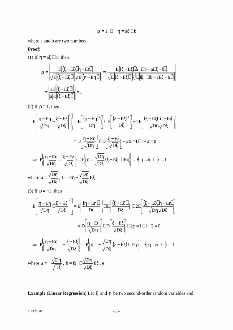
A.BENHARI -36-
1=ρ ⇔ ba +ξ=η
where a and b are two numbers.
Proof:
(1) If ba +ξ=η , then
( )( )[ ]( )[ ] ( )[ ]
( )( )[ ]( )[ ] ( )[ ]2222 baEbaEEE
baEbaEE
EEEE
EEE
−ξ−+ξξ−ξ
−ξ−+ξξ−ξ=η−ηξ−ξ
η−ηξ−ξ=ρ
( )[ ]( )[ ] 1
EEa
EaE2
2
=ξ−ξξ−ξ=
(2) If 1=ρ , then
( ) ( ) ( )( )
ξηη−ηξ−ξ−
ξξ−ξ+
ηη−η=
ξξ−ξ−
ηη−η
DD
EEE2
D
EE
D
EE
D
E
D
EE
222
02112D
ED
D
ED =−+=ρ−
ξξ−ξ+
ηη−η=
⇒ ( ) 1baPEED
DP
D
E
D
EP =+ξ=η=
η+ξ−ξξη
=η=
ξξ−ξ=
ηη−η
where ξη
=D
Da , ξ
ξη
−η= ED
DEb .
(3) If 1−=ρ , then
( ) ( ) ( )( )
ξηη−ηξ−ξ+
ξξ−ξ+
ηη−η=
ξξ−ξ+
ηη−η
DD
EEE2
D
EE
D
EE
D
E
D
EE
222
02112D
ED
D
ED =−+=ρ+
ξξ−ξ+
ηη−η=
⇒ ( ) 1baPEED
DP
D
E
D
EP =+ξ=η=
η+ξ−ξξ
η−=η=
ξξ−ξ−=
ηη−η
where ξη
−=D
Da , ξ
ξη
+η= ED
DEb . #
Example (Linear Regression) Let ξ and η be two second-order random variables and

A.BENHARI -37-
( ) ( )[ ]2baEb,ae +ξ−η=
How to choose a and b to make the error ( )b,ae as small as possible? By taking partial
derivatives of ( )b,ae with respect to a and b, one can have
( ) ( )[ ]( ) [ ]
=−ξ−η−=∂
∂
=ξ−ξ−η−=∂
∂
0baE2b
b,ae
0baE2a
b,ae
⇒ [ ] [ ]
µ=+µ
ξη=µ+ξ
21
12
ba
EbaE ⇒
µ−µ=
ρσσ
=
12
1
2
ab
a
where ξ=µ E1 , η=µ E2 , ξ=σ D1 and η=σ D2 . Let
( ) ( ) 211
2L µ+µ−ξρσσ
=ξ
( )ξL is often called the linear regression of η or linear approximation to η . The error
between a random variable and its linear regression is then given by
( )[ ] ( ) ( )[ ] ( )222
2
12
22min 1aELEe ρ−σ=µ−ξ−µ−η=ξ−η=
If 1±=ρ , ( )[ ] 0LE2 =ξ−η , i.e., ( )ξ=η L . #
3. Conditional Expectations and Regression Analysis
Definition Let η and ξ be two random variables, the conditional expectation of η , given
x=ξ , is then defined as
[ ] ( ) ( )( )∫∫
+∞
∞− ξ
ξη+∞
∞−ξη ==η dy
xf
y,xfydyxyyfxE
Remark: The conditional expectation [ ]xE η is in fact a function of x and [ ]ξηE is then a
function of the random variable ξ . The mean of [ ]ξηE is given by:
[ ][ ] [ ] ( ) ( )( ) ( )∫ ∫∫
∞+
∞−ξ
∞+
∞− ξ
ξη∞+
∞−ξ
=η=ξη dxxfdy
xf
y,xfydxxfxEEE ( ) [ ]η== ∫ ∫
+∞
∞−
+∞
∞−ξη Edydxy,xyf
Example From
( ) 0xyf ≥ξη , ( ) ( )( )
( )( ) 1xf
xfdy
xf
y,xfdyxyf ===
ξ
ξ+∞
∞− ξ
ξη+∞
∞−ξη ∫∫
A.BENHARI -38-
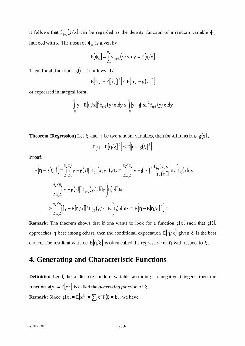
it follows that ( )xyf ξη can be regarded as the density function of a random variable xϕ
indexed with x. The mean of xϕ is given by
[ ] ( ) [ ]xEdyxyyfE x η==ϕ ∫+∞
∞−ξη
Then, for all functions ( )xg , it follows that
[ ][ ] ( )[ ]2
x
2
xx xgEEE −ϕ≤ϕ−ϕ
or expressed in integral form,
[ ] ( ) ( ) ( )∫∫+∞
∞−ξη
+∞
∞−ξη −≤η− dyxyfxgydyxyfxEy
22
Theorem (Regression) Let ξ and η be two random variables, then for all functions ( )xg ,
[ ][ ] ( )[ ]22gEEE ξ−η≤ξη−η .
Proof:
( )[ ] ( ) ( ) ( ) ( )( ) ( )∫ ∫∫ ∫
∞+
∞−ξ
∞+
∞− ξ
ξη∞+
∞−
∞+
∞−ξη
−=−=ξ−η dxxfdy
xf
y,xfxgydydxy,xfxgygE
222
( ) ( ) ( )∫ ∫+∞
∞−ξ
+∞
∞−ξη
−= dxxfdyxyfxgy
2
[ ][ ] ( ) ( ) [ ][ ]22 EEdxxfdyxyfxEy ξη−η=
η−≥ ∫ ∫
+∞
∞−ξ
+∞
∞−ξη #
Remark: The theorem shows that if one wants to look for a function ( )xg such that ( )ξg
approaches η best among others, then the conditional expectation [ ]xE η given ξ is the best
choice. The resultant variable [ ]ξηE is often called the regression of η with respect to ξ .
4. Generating and Characteristic Functions
Definition Let ξ be a discrete random variable assuming nonnegative integers, then the
function ( ) [ ]ξ= xExg is called the generating function of ξ .
Remark: Since ( ) [ ] ( )∑ =ξ== ξ
k
k kPxxExg , we have

A.BENHARI -39-
( ) ( ) ( ) ( )∑ =ξ+−−= −
k
nkn
n
kPx1nk1kkdx
xgdL
⇒ ( ) ( ) ( ) ( ) ( ) ( )[ ]1n1EkP1nk1kk
dx
xgdlim
kn
n
1x+−ξ−ξξ==ξ+−−=∑→
LL
Example Let ξ be a random variable satisfying the binomial distribution, the generating
function of ξ is then given by
( ) [ ] ( )nn
0k
knknk
k qxpqpCxxExg +=== ∑=
−ξ
With the help of ( )xg , one can calculate the moments of ξ :
[ ] ( ) ( ) nppqxpnlimdx
xdglimE 1n
1x1x=+==ξ −
→→
[ ] ( )[ ] [ ] ( ) ( )( ) ( ) npp1nnnppqxp1nnlimnpdx
xgdlimE1EE 222n
1x2
2
1x
2 +−=++−=+=ξ+−ξξ=ξ −
→→
⇒ [ ]( )[ ] [ ] [ ] ( ) ( ) npqp1nppnnpp1nnEEEE 2222222 =−=−+−=ξ−ξ=ξ−ξ=σ
Example Let ξ be a random variable satisfying the Poisson distribution, the generating
function of ξ is then given by
( ) [ ] ( )1xx
0k
kk eeee
!kxxExg −λλ−λ
+∞
=
λ−ξ ==λ== ∑
With the help of ( )xg , one can calculate the moments of ξ :
[ ] ( ) ( ) λ=λ==ξ −λ
→→
1x
1x1xelim
dx
xdglimE
[ ] ( )[ ] [ ] ( ) ( ) λ+λ=λ+λ=λ+=ξ+−ξξ=ξ −λ
→→
21x2
1x2
2
1x
2 elimdx
xgdlimE1EE
⇒ [ ]( )[ ] [ ] [ ] λ=λ−λ+λ=ξ−ξ=ξ−ξ=σ 222222 EEEE
Definition Let ξ be a random variable, then the function ( ) [ ]tjeEt ξ=φ is called the
characteristic function of ξ .
A.BENHARI -40-
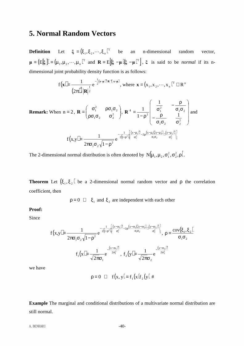
5. Normal Random Vectors
Definition Let ( )Tn21 ,,, ξξξ= Lξ be an n-dimensional random vector,
[ ]( ) ( )Tn21 ,,,E µµµ== Lξµ and ( )( )[ ]TE µξµξR −−= , ξ is said to be normal if its n-
dimensional joint probability density function is as follows:
( )( )
( ) ( )µxRµx
Rx
−−− −
π=
1T
2
1
2
1
2
ne
2
1f , where ( ) nT
n21 Rx,,x,x ∈= Lx
Remark: When 2n = ,
σσρσσρσσ
=2221
2121R ,
σσσρ−
σσρ−
σρ−
=2221
2121
2 1
1
1
11-R and
( ) ( )( ) ( )( ) ( )
σµ−
+σσ
µ−µ−ρ−
σµ−
ρ−−
ρ−σπσ=
22
22
21
2121
21
2
yyx2
x
12
1
221
e12
1x,yf
The 2-dimensional normal distribution is often denoted by ( )ρσσµµ ,,,,N 22
2121 .
Theorem Let ( )21 ,ξξ be a 2-dimensional normal random vector and ρ the correlation
coefficient, then
0=ρ ⇔ 1ξ and 2ξ are independent with each other
Proof:
Since
( ) ( )( ) ( )( ) ( )
σ−+
σσ−−ρ−
σ−
ρ−−
ρ−σπσ=
22
22
21
2121
21
2
mymymx2
mx
12
1
221
e12
1x,yf ,
( )21
21,cov
σσξξ=ρ
( )( )
21
21
2
mx
1
1 e2
1xf σ
−−
σπ= , ( )
( )22
22
2
my
2
2 e2
1yf σ
−−
σπ=
we have
0=ρ ⇔ ( ) ( ) ( )yfxfy,xf 21= #
Example The marginal and conditional distributions of a multivariate normal distribution are
still normal.
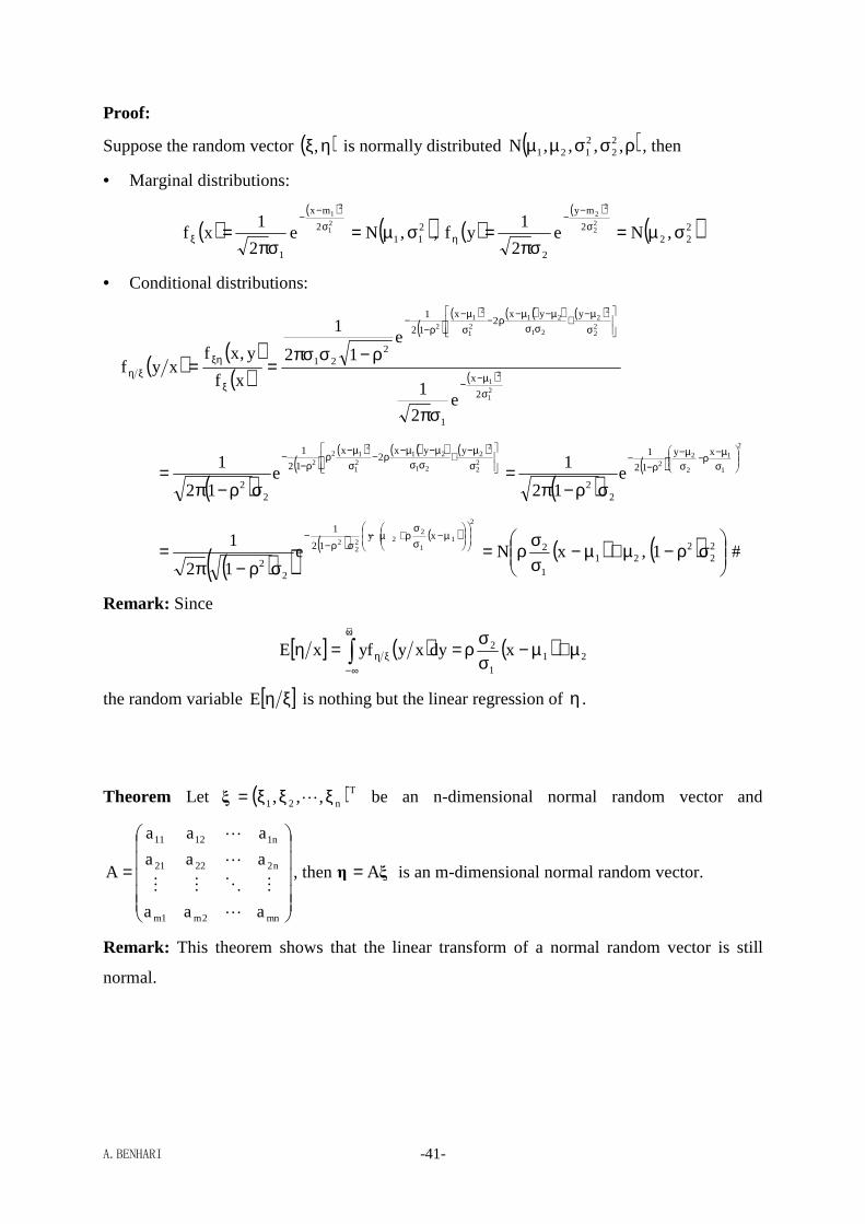
A.BENHARI -41-
Proof:
Suppose the random vector ( )ηξ, is normally distributed ( )ρσσµµ ,,,,N 22
2121 , then
• Marginal distributions:
( )( )
( )211
2
mx
1
,Ne2
1xf
21
21
σµ=σπ
= σ−
−
ξ , ( )( )
( )222
2
my
2
,Ne2
1yf
22
22
σµ=σπ
= σ−
−
η
• Conditional distributions:
( ) ( )( )
( )( ) ( )( ) ( )
( )21
21
22
22
21
2121
21
2
2
x
1
yyx2
x
12
1
221
e2
1
e12
1
xf
y,xfxyf
σµ−−
σµ−
+σσ
µ−µ−ρ−
σµ−
ρ−−
ξ
ξηξη
σπ
ρ−σπσ==
( )( )
( ) ( )( ) ( )
( )( )
2
1
1
2
222
2
22
21
2121
212
2xy
12
1
22
yyx2
x
12
1
22
e12
1e
12
1
σµ−ρ−
σµ−
ρ−−
σµ−+
σσµ−µ−ρ−
σµ−ρ
ρ−−
σρ−π=
σρ−π=
( )( )( ) ( )
( ) ( )
σρ−µ+µ−
σσρ=
σρ−π=
µ−
σσ
ρ+µ−σρ−
−22
221
1
2xy
12
1
22
1,xNe12
12
11
222
22
#
Remark: Since
[ ] ( ) ( ) 211
2 xdyxyyfxE µ+µ−σσρ==η ∫
+∞
∞−ξη
the random variable [ ]ξηE is nothing but the linear regression of η.
Theorem Let ( )Tn21 ,,, ξξξ= Lξ be an n-dimensional normal random vector and
=
mn2m1m
n22221
n11211
aaa
aaa
aaa
A
L
MOMM
L
L
, then ξη A= is an m-dimensional normal random vector.
Remark: This theorem shows that the linear transform of a normal random vector is still
normal.
A.BENHARI -42-
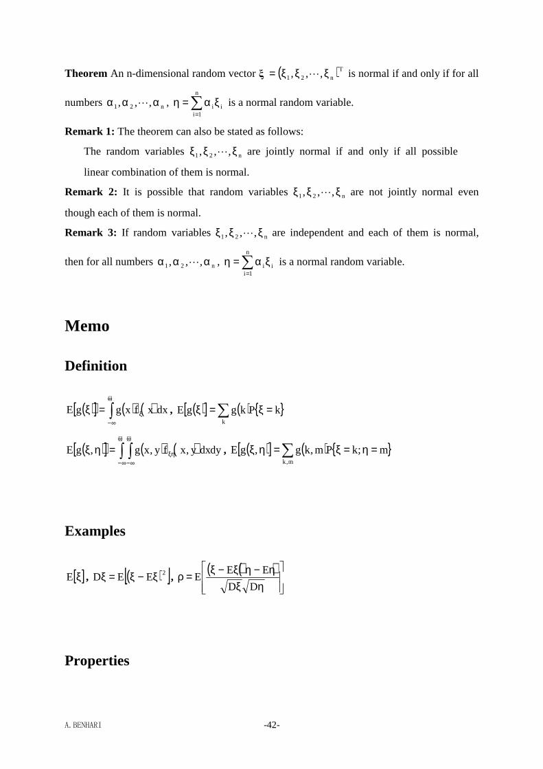
Theorem An n-dimensional random vector ( )Tn21 ,,, ξξξ= Lξ is normal if and only if for all
numbers n21 ,,, ααα L , ∑=
ξα=ηn
1iii is a normal random variable.
Remark 1: The theorem can also be stated as follows:
The random variables n21 ,,, ξξξ L are jointly normal if and only if all possible
linear combination of them is normal.
Remark 2: It is possible that random variables n21 ,,, ξξξ L are not jointly normal even
though each of them is normal.
Remark 3: If random variables n21 ,,, ξξξ L are independent and each of them is normal,
then for all numbers n21 ,,, ααα L , ∑=
ξα=ηn
1iii is a normal random variable.
Memo
Definition
( )[ ] ( ) ( )∫+∞
∞−ξ=ξ dxxfxggE , ( )[ ] ( ) kPkggE
k
=ξ=ξ ∑
( )[ ] ( ) ( )∫ ∫+∞
∞−
+∞
∞−ξη=ηξ dydxy,xfy,xg,gE , ( )[ ] ( ) m;kPm,kg,gE
m,k
=η=ξ=ηξ ∑
Examples
[ ]ξE , ( )[ ]2EED ξ−ξ=ξ , ( )( )
ηξη−ηξ−ξ=ρ
DD
EEE
Properties
A.BENHARI -43-
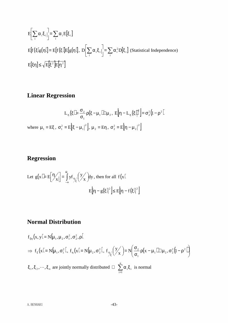
[ ]∑∑ ξα=
ξαi
iii
ii EE
( ) ( )[ ] ( )[ ] ( )[ ]ηξ=ηξ gEfEgfE , [ ]∑∑ ξα=
ξαi
i2i
iii DD (Statistical Independence)
[ ] [ ] [ ]22 EEE ηξ≤ξη
Linear Regression
( ) ( ) 211
2L µ+µ−ξρσσ
=ξη , ( )[ ] ( )222
21LE ρ−σ=ξ−η η
where ξ=µ E1 , [ ]2
121 E µ−ξ=σ , η=µ E2 , [ ]2
222 E µ−η=σ
Regression
Let ( ) ∫+∞
∞− ξη
=
η= dyx
yyfxExg , then for all ( )xf
( )[ ] ( )[ ]22fEgE ξ−η≤ξ−η
Normal Distribution
( ) ( )ρσσµµ=ξη ,,,,Ny,xf 22
2121
⇒ ( ) ( )211,Nxf σµ=ξ , ( ) ( )2
22 ,Nxf σµ=η , ( ) ( )
ρ−σµ+µ−ρ
σσ
=
ξη
22221
1
2 1,xNxyf
n21 ,,, ξξξ L are jointly normally distributed ⇔ ∑=
ξαn
1iii is normal
A.BENHARI -44-
Limit Theorems
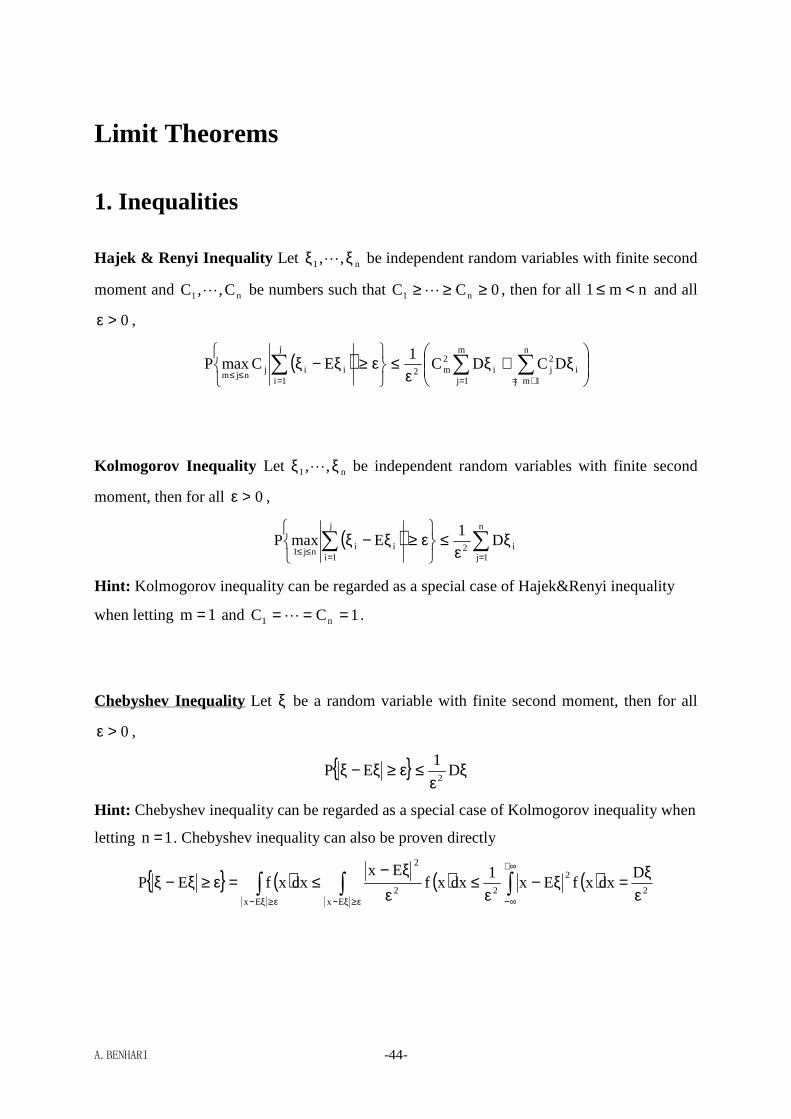
1. Inequalities
Hajek & Renyi Inequality Let n1 ,, ξξ L be independent random variables with finite second
moment and n1 C,,C L be numbers such that 0CC n1 ≥≥≥L , then for all nm1 <≤ and all
0>ε ,
( )
ξ+ξ
ε≤
ε≥ξ−ξ ∑∑∑+===≤≤
n
1mji
2j
m
1ji
2m2
j
1iiij
njmDCDC
1ECmaxP
Kolmogorov Inequality Let n1 ,, ξξ L be independent random variables with finite second
moment, then for all 0>ε ,
( ) ∑∑==≤≤
ξε
≤
ε≥ξ−ξn
1ji2
j
1iii
nj1D
1EmaxP
Hint: Kolmogorov inequality can be regarded as a special case of Hajek&Renyi inequality
when letting 1m = and 1CC n1 ===L .
Chebyshev Inequality Let ξ be a random variable with finite second moment, then for all
0>ε ,
ξε
≤ε≥ξ−ξ D1
EP2
Hint: Chebyshev inequality can be regarded as a special case of Kolmogorov inequality when
letting 1n = . Chebyshev inequality can also be proven directly
( ) ( ) ( )2
2
2Ex
2
2
Ex
DdxxfEx
1dxxf
ExdxxfEP
εξ=ξ−
ε≤
εξ−
≤=ε≥ξ−ξ ∫∫∫∞+
∞−ε≥ξ−ε≥ξ−

A.BENHARI -45-
2. Convergences of Sequences of Random Variables
Convergence in Almost Everywhere A sequence of random variables LL ,,, n1 ξξ is said to
converge almost everywhere to a random variable ξ if
( ) ( ) 1lim,P nn
=ωξ=ωξΩ∈ωω+∞→
Convergence in Probability A sequence of random variables LL ,,, n1 ξξ is said to
converge in probability to a random variable ξ if for all 0>ε ,
( ) ( ) 0,Plim nn
=ε≥ωξ−ωξΩ∈ωω+∞→
Convergence in Distribution A sequence of random variables LL ,,, n1 ξξ is said to
converge in distribution to a random variable ξ if for all x at which ( )xF is continuous,
( ) ( )xFxFlim nn
=+∞→
where ( )xF and ( )xFn are distribution functions of ξ and nξ , L,2,1n = , respectively.
Remark: Note that
( ) ( )xFxFlim nn
=+∞→
⇔ ( ) ( ) x,Px,Plim nn
<ωξΩ∈ωω=<ωξΩ∈ωω+∞→
Convergence in the rth mean/moment A sequence of random variables LL ,,, n1 ξξ is said
to converge in the rth mean/moment to a random variable ξ if
[ ] 0Elimr
nn
=ξ−ξ+∞→
Remark: If 2r = , the convergence is the well-known mean square convergence.
The relation between different types of convergence
Convergence Almost Everywhere ⇒ Convergence in Probability
⇒ Convergence in Distribution

A.BENHARI -46-
3. The Weak Laws of Large Numbers
Definition A sequence of random variables LL ,,,, n21 ξξξ is said to satisfy the weak law of
large numbers if there is a sequence of numbers LL ,a,,a,a n21 such that for all 0>ε
0an
1Plim n
n
1kk
n=
ε≥−ξ∑=+∞→
Remark: The convergence involved in the weak laws of larger numbers is exactly the type of
convergence in probability. In fact, let n
n
1kkn a
n
1 −ξ=η ∑=
, L,2,1n = , then
0Pliman
1Plim n
nn
n
1kk
n=ε≥η=
ε≥−ξ+∞→=+∞→ ∑
This means that the sequence of random variables LL ,,,, n21 ηηη converges in probability to
zero.
Theorem (The Weak Law of Large Numbers, Khintchine) Suppose the second-order
random variables LL ,,,, n21 ξξξ are independent and identically distributed, then for all
0>ε ,
0n
1Plim
n
1kk
n=
ε≥µ−ξ∑=+∞→
where [ ]kE ξ=µ .
Proof:
0n
nE
nP
n2
2
2
2n
1k
k
InequalityChebyshev
n
1k
k →ε
σ=ε
µ−ξ
≤
ε≥µ−ξ
+∞→
=
=
∑∑
where ( )[ ]2k
2 E µ−ξ=σ . #

A.BENHARI -47-
4. The Strong Laws of Large Numbers
Definition A sequence of random variables LL ,,,, n21 ξξξ is said to satisfy the strong law of
large numbers if there is a sequence of numbers LL ,a,,a,a n21 such that for all 0>ε
10an
1limP n
n
1kk
n=
=
−ξ∑=+∞→
Remark 1: The convergence involved in the strong laws of larger numbers is exactly the type
of convergence almost everywhere. In fact, let n
n
1kkn a
n
1 −ξ=η ∑=
, L,2,1n = , then
10limP0an
1limP n
nn
n
1kk
n==η=
=
−ξ+∞→=+∞→ ∑
This means that the sequence of random variables LL ,,,, n21 ηηη converges almost
everywhere to zero.
Remark 2: Since the convergence almost everywhere will lead to the convergence in
probability, a sequence of random variables satisfying the strong laws of large number must
satisfy the weak ones:
10an
1limP n
n
1kk
n=
=
−ξ∑=+∞→
⇒ 0an
1Plim n
n
1kk
n=
ε≥−ξ∑=+∞→
for all 0>ε
Theorem (The Strong Law of Large Numbers, Kolmogorov) Suppose the second-order
random variables LL ,,,, n21 ξξξ are independent with each other and +∞<ξ
∑+∞
=1n2k
n
D, then
( )10a
n
1limP0
n
ElimP n
n
1kk
nEn
1a
n
1kkk
n n
1kkn
=
=
−ξ=
=ξ−ξ
∑∑
=+∞→∑ ξ=
=
+∞→=
Theorem (The Strong Law of Large Numbers, Khintchine) Suppose the second-order
random variables LL ,,,, k21 ξξξ are independent and identically distributed, then
A.BENHARI -48-
1n
1limP
n
1kk
n=
µ=ξ∑
=+∞→
where kEξ=µ .
Hint: Since the random variables LL ,,,, k21 ξξξ are identically distributed, one can have
+∞<ξ=ξ
∑∑+∞
=
+∞
= 1k2k
1k2k
k
1D
k
D
Remark: If kξ satisfies the 0-1 distribution:
=α−=α
=α=ξ0p1
1pP k , then
pE k =ξ and 1pn
1limP
n
1kk
n=
=ξ∑
=+∞→
Note that ∑=
ξn
1kkn
1 represents the frequency of occurrence of the event 1k =ξ in n Bernoulli
experiments, the law of large numbers implies that the frequency will approximate the
corresponding probability p as +∞→n .

A.BENHARI -49-
5. The Central Limit Theorems
Let LL ,,,, i21 ξξξ be a sequence of independent random variables with finite second
moments and
ξ
ξ−ξ=η
∑
∑∑
=
==
n
1ii
n
1ii
n
1ii
n
D
E, L,2,1n = , the central limit theorems are concerned with
the conditions under which the distribution of nη will tend to the standard normal distribution
( )1,0N as +∞→n , i.e.,
∫∞−
−
+∞→ π=<η
x
2
t
nn
dte2
1xPlim
2
Remark 1: Note that nη is the standardized variable of ∑=
ξn
1ii .
Remark 2: The convergence involved in the central limit theorems is exactly the type of
convergence in distribution. In fact, let ( ) ∫∞−
−
π=Φ
x
2
t
dte2
1x
2
and ( ) xPx nn <η=Φ ,
L,2,1n = , then
∫∞−
−
+∞→ π=<η
x
2
t
nn
dte2
1xPlim
2
⇔ ( ) ( )xxlim nn
Φ=Φ+∞→
The Central Limit Theorem (Lindeberg & Levi Theorem) Let LL ,,,, n21 ξξξ be a
sequence of independent and identically distributed (IID) random variables with finite second
moment, then,
∫∞−
−
+∞→ π=<η
x
2
t
nn
dte2
1xPlim
2
where σ
µ−ξ=
ξ
ξ−ξ=η
∑
∑
∑∑=
=
==
n
n
D
En
1ii
n
1ii
n
1ii
n
1ii
n , iEξ=µ , i2 Dξ=σ .

A.BENHARI -50-
The Central Limit Theorem (de Moivre & Laplace Theorem) Let LL ,,,, n21 ξξξ be a
sequence of IID random variables with finite second moment, if
==−=
==ξ0kqp1
1kpkP i for all i, then,
1
enpq2
1
kP
lim 2
npq
npk
2
1
n
1ii
n=
π
=ξ
−−
=
+∞→
∑ , ∫
∑
∞−
−=
+∞→ π=
<−ξ x
2
t
n
1ii
ndte
2
1x
npq
npPlim
2
Remark: For the approximation calculation of ∑=
ξn
1ii , we so far have
( ) np
kn
1ii e
!k
npkP −
=
≈
=ξ∑ , when n is large enough and p is small enough
2
npq
npk
2
1n
1ii e
npq2
1kP
−−
= π≈
=ξ∑ , when n is large enough
∫∑
∞−
−=
π≈
<−ξ x
2
t
n
1ii
dte2
1x
npq
npP
2
, when n is large enough. In this case, npq
npn
1ii −ξ∑
=
can be regarded as a standard normal variable, which leads to
∫∑
∑
−
−
−=
= π≈
−<−ξ
≤−=
<ξ≤
npq
npx
npq
np
2
t
n
1iin
1ii dte
2
1x
npq
npx
npq
np
npq
npPx0P
2
A.BENHARI -51-
Conditioning. Conditioned distribution and expectation.
1. The conditioned probability and expectation. 1. The conditioned probability and expectation. 1. The conditioned probability and expectation. 1. The conditioned probability and expectation.
Let (Ω, K, P) be a probability space. Let A ∈ K be an event such that P(A) ≠ 0. Let B be another event from K. Define
(1.1) P(B A) = )(
)(
AP
BAP
This is called the conditioned probability of B given A.
Of course that P(BA) = P(B) ⇔ P(BA) = P(B)P(A) ⇔ A and B are independent.
If A is given, we may consider the function PA : K → [0,1] given by
(1.2) PA(B) = P(BA) It is obvious that PA is a new probability on the σ-algebra K, called the
conditioned probability given A.
The integral of a random variable X with respect to it will be denoted by
E(XA) or EA
(X). The computing formula is
PROPOSITION 1.1. E(XA) = )(
)1(
AP
XE A
Proof. Obvious for X = 1B
. Then apply the usual method of four steps: X simple,
X nonnegative, X any.
Let now Y be a discrete random variable and I be the set y ∈ ℜ P(Y = y) ≠ 0. Then I is at most countable and Y admits the cannonic representation
∑∈
==Iy
yYyY 1 (a.s.) . In many statistical problems one gets interested in
computing the probability of an event B if one has an information about Y. In
other words one wants to know P(B Y = y). It is natural to define P(B Y) as (1.3) P(B Y) = ∑
∈Iy
P(B Y = y)1Y = y .
This quantity will be called the conditioned probability of B given the random
variable Y.
EXAMPLE.. An urn I has n labelled balls (that is I =1,2,..,n. One draws two
balls without replacing. The first one is Y and the second one is X . One wants to
compute P(X=x Y) and to compare it with P(X = x ) . Accepting that we are in the classical context , Ω = I
2
\ (i,i)i ∈ I , thus Ω= n(n-1) . Then P(X = x
Y = y ) =
)(
),(
yYP
yYxXP
===
=
yY
yYxX
=== ,
=
≠−
=
yxifn
yxif
1
10
(as Y has only n -1
possibilities). It means that
P(X=x Y) = ∑∈ xIy \
1
1
−n1Y = y =
1
1
−n1Y ≠ x . Compare this with P(X=x) =
n
1.
Looking at (1.3) one remarks four things :(i). the conditioned probability is a
random variable ; (ii). the random variable does not depend as much on Y as on the

A.BENHARI -52-
sets Y=y which form a partition of Ω ;(iii). This random variable is measurable
with respect to the σ-algebra σ(Y) := Y-1
(BBBB(ℜ)) and, finally, (iv). The random
variable may be not defined everywhere, but only almost surely : if P(Y=y) = 0,
then P(B Y=y) may be any number form 0 to 1. A convention, as good as any other, would be that in this case to decree that P(B Y=y)=0.
It means that a more “natural” definition would be the conditioned probability
of B given a partition ∆ = (∆j) j ∈ I where I is at most countable . Then the analog
of (1.3) would be
(1.4) P(B ∆ ) = ∑≠∆
∆∆0)(:
1)(j
jPj
jBP
Taking into account Proposition 1. one is suggested to define
(1.5) E(X ∆) = ∑≠∆
∆∆0)(:
1)(j
jPj
jXE , X ∈ L
1
(the condition that X ∈ L
1
means that E X < ∞ ; it is not necessary, but
makes things easier)
The definition (1.5) has the advantage that E(1B ∆) = P(B ∆ ) , as it is normal to be .
We want to generalize the definition (1.5) in other situations. The most
general situation is when we replace “partition” by “σ-algebra” . If in (1.5) we
denote by F the σ-algebra given by by ∆ (remark that A ∈ F ⇔ A = UJj
j∈
∆ for some
J ⊂ I ) , we can say that the right hand of (5) is a definition for E(XF) ,
instead of E(X ∆). So
(1.6) E(X F F F F ) = ∑≠∆
∆∆0)(:
1)(j
jPj
jXE , X ∈ L
1
What properties characterize the dfinition (1.6) which can be generalized to
an arbitray sub-σ-algebra of K?
Remark that if we denote by Y the right hand of (1.6), then
(i). Y is FFFF –measurable ; moreover, Y ∈ L
1
(Ω, FFFF, P) (ii). If A ∈ F then E(X1A) = E(Y1A)
Indeed, Y1 = EY ≤ ∑∈
∆∆Ij
j jXEE 1)( ≤ ∑
≠∆∆∆
0)(:
)1)((j
jPj
jXEE = EX < ∞. As
about the claim (ii) , let A ∈ F ⇔ A = UJj
j∈
∆ for some J ⊂ I. Then E(Y1A) =
∑∈
∆Jj
jYE )1( (by Lebesgue’s dominated convergence) = )1)((∑
∈∆∆
Jjj j
XEE (since ∆j are
disjoint) = )()(∑∈
∆∆Jj
jj PXE = )1(∑∈
∆Jj
jXE (by Proposition 1) = E(X1A).
The conditions (i) and (ii) are used to define E(X F F F F ) in general situations.
DefinitionDefinitionDefinitionDefinition.1111. Let X ∈ L
1
(Ω,KKKK,P) and FFFF⊂ KKKK be a sub σ-algebra. We say that Y = E(X FFFF) (read : Y is the conditioned expectation of X given FFFF ) iff (1.7) Y is FFFF –measurable and A ∈ FFFF ⇒ E(X1A) = E(Y1A)
Definition.Definition.Definition.Definition.2. 2. 2. 2. Let B ∈ KKKK . By P(B KKKK) we shall understand E(1B F F F F ). Read: “the

A.BENHARI -53-
conditioned probability of B given F F F F ”.
Definition. 3. Definition. 3. Definition. 3. Definition. 3. Let X be a random variable and FFFF⊂ KKKK be a sub σ-algebra. By PoX-
1
(BF F F F ) we shall understand the random variable P(X-1
(B) FFFF). Read: “ the
conditioned distribution of X given FFFF ” .
One may remark that the key concept is that of conditioned expectation.
2. Properties of the conditioned expectation. 2. Properties of the conditioned expectation. 2. Properties of the conditioned expectation. 2. Properties of the conditioned expectation.
Property Property Property Property 1. Almost sure unicity. Almost sure unicity. Almost sure unicity. Almost sure unicity. If X is an integrable r.v., then E(XFFFF) exists and is unique a.s. , i.e. if Y1 and Y2 are two versions of E(XFFFF), then Y1 = Y2
(a.s.)
Proof. The signed measure X⋅P : FFFF → ℜ is absolutely continuous with respect to P
, since P(A)=0 ⇒ (X⋅P)(A) = ∫ X1AdP = 0 (as X1A = 0 a.s.). The Radon Nikodym
theorem says that there must be a density of X⋅P with respect to P : there must exist Y which is FFFF –measurable such that X⋅P = Y⋅P . Notice that we think both measures living on the σ-algebra FFFF. The unicity is guaranteed by the same Radon Nikodym theorem; but one may check it directly, as an exercise. If Y1⋅P = Y2⋅P , the meaning is that ∫ (Y1-Y2)1A dP = 0 ∀ A ∈ F F F F ; one may as well choose A =Y1>Y2=
U∞
=
+>
121
1
n nYY and get that P(Y1>Y2) = 0. In the same way one gets that P(Y1<Y2) =
0, that is P(Y1≠Y2)=0 ⇔ Y1 = Y2 (a.s.).
Property Property Property Property 2. Generalizing the usual expectation.Generalizing the usual expectation.Generalizing the usual expectation.Generalizing the usual expectation. Suppose that is FFFF is trivial, meaning that A ∈ FFFF ⇒ P(A) ∈0,1. Then E(XFFFF) = EX. Moreover, if X is already FFFF –measurable, then E(XFFFF) = EX. It means that the FFFF- measurable functions behave as the constants do, in the usual case.
Proof. Let Y = E(XFFFF) . As Y is FFFF- measurable, Y must be a constant a.s. Indeed, the sets Lb=Y < b ∈ FFFF. They are an increasing family, in the sense that
b < c ⇒ Lb⊂Lc.Their probability can be either 0, or 1. As 0 = P(∩bLb) = limb→-
∞P(Lb) it means that some of these sets will heve probability 0. Let c = sup b ∈
ℜ P(Lb) = 0. Then, due to the definition of c, P(Lc+ε ) = 1 ∀ ε > 0. In the same way P(Lc) = 0. By the monotonous continuity of any measure it follows that P(Y ≤ c) = 1 but P(Y<c) = 0 ⇔ P (Y = c) = 1 ⇔ Y = c (a.s.). So Y is a constant a.s.
If in (1.7) we take A = Ω , we get that EX = E(X1A) = E(Y1A) = EY = Ec = c.
As about the second claim, it is obvious from 1.7.
Property Property Property Property 3. ProjectivityProjectivityProjectivityProjectivity. If FFFF ⊂ G G G G are two σ-algebras then E(E(XGGGG)F F F F )=E(XF F F F ). As a consequence of property 2, we get that EX = E(E(XGGGG)).
Proof. Let Y = E(XG G G G ) and Z = E(XF F F F ). We want to check that E(Y FFFF) = Z . Firstly, Z is FFFF – measurable. Secondly, let A ∈ FFFF. Then E(Z1A) = E(X1A) (by 1.7) =
E(Y1A) (again by 1.7; notice that A ∈ FFFF ⇒ A ∈ GGGG ! ) It means that E(Y FFFF) = Z.
A.BENHARI -54-
Property Property Property Property 4. LinearityLinearityLinearityLinearity. If a,b ∈ ℜ and X1,X2 ∈ L
1
then E(aX1+bX2F F F F ) = aE(X1F F F F )+bE(X2F F F F ) (a.s.) Proof. Let Yj = E(XjF F F F ), j = 1,2. Let Y = aY1+bY2 and A ∈ FFFF . Then Y is FFFF –
measurable and, moreover, E(Y1A) = E((aY1+bY2 )1A) =a E(Y1 1A) +b E(Y2 1A) = a E(X1 1A)
+b E(X2 1A) (by 1.7) = E((aX1+bX2 )1A) , checking the second condition from 1.7.
Property Property Property Property 5. MonotonicityMonotonicityMonotonicityMonotonicity. If X1 ≤ X2 then E(X1F F F F ) ≤ bE(X2F F F F ) (a.s.) Proof. Using Property 4, it is enough to check that X ≥ 0 ⇒ E(XF F F F ) ≥ 0 (a.s.). Let Y = E(XF F F F ) . Y is FFFF – measurable and A ∈ FFFF ⇒ E(Y1A) = E(X1A) ≥ 0 – since X
≥ 0. If one puts A = Y<0 it follows that E(Y1A) = -E(Y-) ≥ 0 ⇒ E(Y-) ≤ 0 ⇒ E(Y-)
= 0 (a.s.) ⇒ Y = Y+ (a.s.) ⇒ Y ≥ 0 (a.s.) .
Property Property Property Property 6. JensenJensenJensenJensen’s inequalitys inequalitys inequalitys inequality. Let X : Ω → I ⊂ ℜ be a random variable and f :
I → ℜ be convex (here I is an interval!). Then E(f(X)F F F F ) ≥ f(E(XF F F F )). Proof. A convex function f can be written as f = sup haa ∈ Γ, Γ at most countable and ha affine functions, ha(x) = max+na. (for instance Γ = Q∩I and if a ∈
Γ, ha is a tangent for f at (a, f(a)) ; it is known that a convex function has at
least one tangent at every point)
Then E(f(X)F F F F ) = E(sup ha(X)a ∈ ΓF F F F ) ≥ sup E(ha(X)FFFF)a ∈ Γ (by Property 6, monotonicity) = sup E(maX+na)FFFF)a ∈ Γ= sup maE( XF F F F ) + naa ∈ Γ (by linearity and Property 2 – the expectation of a constant is the constant itself) = f(E(XFFFF)).
Property 7Property 7Property 7Property 7. ContractivityContractivityContractivityContractivity. Let p∈[1,∞] and X ∈ L
p
. Then E(XF F F F )p ≤ Xp.
As a consequence the conditioned expectation is a linear contraction from
L
p
(Ω,KKKK,P) to L
p
(Ω,FFFF,P) Proof. There are two cases.
1. 1≤p < ∞. The claim is EE(XF F F F )p
≤ EXp
. Let f(x) = xp
. Then f : ℜ →
ℜ is convex so we know that E(f(X)F F F F ) ≥ f(E(XF F F F )) ⇔ E(XpF F F F ) ≥ E(XF F F F )p
. If we take the expectation, we get E(E(XpF F F F )) ≥ E(E(XF F F F )p
) which, because of Property 3 is exactly our claim.
2. p = ∞. Let then M = X∞ . It means that X≤ M (a.s.) ⇒ E(X F F F F ) ≤ E(MF F F F ) (by property 5, monotonicity) ⇒ E(X F F F F ) ≤ M (a.s.) ⇒
E(X F F F F )∞ ≤ M .
Property Property Property Property 8888. Conditioned BeppoConditioned BeppoConditioned BeppoConditioned Beppo----Levi, Fatou and Lebesgue theorems.Levi, Fatou and Lebesgue theorems.Levi, Fatou and Lebesgue theorems.Levi, Fatou and Lebesgue theorems. Precisely, the
claim runs as follows:
1. If Xn ≥ g ∈ L
1
and Xn ↑X (or Xn↓X, Xn ≤ g ∈ L
1
) then E(XnF F F F ) ↑ E(XF F F F ) (a.s.) (or E(XnF F F F ) ↓ E(XF F F F ) (a.s.)). (Beppo – Levi);
2. If Xn ≥ g ∈ L
1
(resp. Xn ≤ g ∈ L
1
) then E(liminfn→∞ XnF F F F ) ≤ liminfn→∞ E(Xn
F F F F )(resp. E(limsupn→∞ XnF F F F ) ≥ limsupn→∞ E(Xn F F F F ) (Fatou) ; 3. If Xn → X (a.s.) and Xn ≤ g ∈ L
1
, then a.s.-lim E(XnF F F F ) = E(XF F F F ) (Dominated convergence, Lebesgue)
A.BENHARI -55-
Proof. Let Yn = E(XnF F F F ). Due to monotonicity, Yn is almost surely increasing. Let Y
be its supremum , which is a.s. the same with its limit. The claim is that Y =
E(XF F F F ). According to (1.7) what we have to do is to check the measurability (obvious) and the fact that A ∈ FFFF ⇒E(X1A) = E(Y1A). But E(X1A) = E(↑limXn1A) =
↑limE(Xn1A) (usual Beppo-Levi) = ↑limE(Yn1A) (by (1.7)) = E(↑limYn1A) (again Beppo
Levi) = E(Y1A) . That checks property 1.
As about 2., the proof is the same as in the usual case, (monotonicity and
conditioned Beppo-Levi) : E(liminfn→∞ XnF F F F ) = E(supn infk Xn+kF F F F ) = E(supn YnF F F F ) (with Yn = infk Xn+k, an increasing sequence) = E(↑limYnFFFF) = ↑limE(YnF F F F ) (conditioned Beppo-Levi) = supnE(infk Xn+kF F F F ) ≤ supn infk E(Xn+kF F F F ) (monotonicity) = liminfn→∞ E(Xn F F F F ). The conditioned Lebesgue theorem puts no problems: so X = liminfn→∞ Xn = limsupn→∞Xn
. we apply conditioned Fatou’s lemma : limsupn→∞ E(XnF F F F ) ≤ E(limsupn→∞XnFFFF)= E(XF F F F ) = E(liminfn→∞XnF F F F )≤ liminfn→∞ E(Xn
F F F F ) meaning that limsupn→∞ E(XnF F F F ) = liminfn→∞ E(Xn F F F F ) = E(XF F F F ).
Property Property Property Property 9. 9. 9. 9. The The The The FFFF----measurable functions behave as constants.measurable functions behave as constants.measurable functions behave as constants.measurable functions behave as constants.
Precisely, the property runs as follows: if X ∈L
p
and Y ∈L
q
, with 111 =+qp
, p,q
≥ 1, then E(XYF F F F ) = YE(XF F F F ). Remark that if F F F F is trivial then Y is a constant. Proof. The condition X ∈L
p
and Y ∈L
q
is put for convenience, what we want is that
XY ∈ L
1
.
The proof will be standard. Let Z = YE(XF F F F ). Our claim means that Z is F F F F – measurable (obvious) and that A ∈F F F F ⇒ E(XY1A) = E(Z1A) .
Step 1. Y = 1B, B ∈FFFF . Then E(Z1A) = E(YE(XF F F F )1A) = E(E(XF F F F )1A1B) = E(E(XF F F F )1A∩B)
= E(X1A∩B) (as A,B ∈ FFFF ⇒ A∩B ∈ FFFF , too!) = E(X1A1B) = E(XY1A) so in this case we
are done.
Step 2. Y is simple, i.e. Y = ∑=
n
iBi i
b1
1 , Bi ∈FFFF . Then E(Z1A) = E(YE(XF F F F )1A) =
∑=
n
iBAi i
Eb1
11( E(XF F F F )) = ∑=
n
iBAi i
XEb1
11( F F F F ) (by step 1!) = ∑=
n
iBiA i
bXE1
11( F F F F ) (by
linearity) = E(XY1A) finishing the proof in this case, too.
Step 3. Y is nonnegative. Then Y is the limit of a nondecreasing sequence of
simple functions, Yn. We have: E(Z1A) = E(YE(XF F F F )1A) = E(YE(X+F F F F )1A) - E(YE(X-F F F F )1A) = E(↑limnYnE(X+F F F F )1A) - E(↑limnYnE(X-F F F F )1A) = ↑limn E(YnE(X+F F F F )1A) - ↑limn
E(YnE(X-F F F F )1A) (Beppo-Levi!) =↑limn E(E(X+Yn1AF F F F ) - ↑limn E(E(X-Yn1AF F F F ) (Step 2! Yn1A is simple!) =↑limn E(X+Yn1A) - ↑limn E(X-Yn1A ) (Property 3!) = E(X+↑limn Yn1A)
- E(X-↑limn Yn1A ) (Beppo Levi again!) = E(X+Y1A) - E(X-Y1A ) = E((X+-X-)Y1A) =
E(XY1A) .
Step 4. Y is any. Then Y = Y+ -Y- hence E(Z1A) = E(YE(XF F F F )1A)
= E(Y+ E(XF F F F )1A) - E(Y- E(XF F F F )1A) = E(E(X Y+1A F F F F )) - E(E(X Y-1A F F F F )) (by step 3 ! Y+1A and Y-1A are nonnegative) = E(X Y+1A) - E(X Y-1A ) (property 3) = E(X( Y+-Y-)1A
) = E(XY1A) .
A.BENHARI -56-
Property Property Property Property 10101010. Optimality. Optimality. Optimality. Optimality. Let X ∈ L
2
. Consider the function D: L
2
(Ω,FFFF,P) → [0,∞)
given by
D(Y) = X-Y2 . Then D is convex and has an unique (a.s.) point of minimum which
is exactly Y = E(XF F F F ). Moreover, the following Pythagora rule holds:
X-Y2
2
= X-Y2
2
+
Y- E(XF F F F ) 2
2
.
As a consequence the mapping E
FFFF : L
2
→ L
2
(Ω,FFFF,P) given by EFFFF (X) = E(XF F F F ) is the
orthogonal projector from the Hilbert space L
2
to the Hilbert subspace L
2
(Ω,FFFF,P).
Proof. Let Z= E(XF F F F ). Then X-Y2
2
= E(X-Y)
2
= E((X-Z)+(Z-Y))
2
=
E((X-Z)
2
) + E((Z-Y)
2
+ 2 E((X-Z)(Z-Y)) . The last term is equal to 2 E(E((X-Z)(Z-
Y)F F F F )) (property 3) = 2E((Z-Y) E((X-Z)F F F F )) = 2E((Z-Y) (E(XF F F F )-Z)) = 2E((Z-Y)
(Z-Z)) = 0. It means that X-Y2
2
= X-Y2
2
+
Z-Y2
2
.
Property Property Property Property 11. 11. 11. 11. Conditioning and independence. Conditioning and independence. Conditioning and independence. Conditioning and independence. If X is independent on FFFF , then E(XFFFF) = EX . It is not true in general that E(XFFFF) = EX ⇒ X is independent on FFFF . However, if P(BF F F F ) = const ⇔ P(BF F F F ) = P(B) ⇔ B is independent on FFFF . Proof. Let X be independent on FFFF and Y = EX. The task is to prove that Y fulfills the conditions (1.7). As measurability is obvious, let A ∈ FFFF (hence A is independent on X ⇔ X and 1A are independent) Then E(X1A) = EX ⋅ E1A = EX⋅P(A) = E(EX⋅1A) = E(Y1A) checking the first claim. As about the converse, it cannot be
true since it is enough to choose X = 1A – 1B with P(A) = P(B) = p and FFFF =σ(∆) where ∆ = (∆j)j∈J is an (at most) countable partition of Ω. Then EX = 0 and
E(XFFFF) = P(AFFFF ) – P(BF F F F ) = ( )j
Jjjj BPAP ∆
∈∑ ∆−∆ 1()( . If we choose A and B such
that P(A∆j) = P(B∆j) ≠ pP(∆j) , that would be an example that it is possible that
E(XFFFF) = EX = 0 but X be not independent on FFFF, since P(X=1,∆j) = P(A∆j) ≠ P(X=1)P(∆j).
However, suppose that P(BF F F F ) = c where c is a constant. By (1.7) this means that E(1A1B) = E(c1A) ∀ A ∈ FFFF, or that P(AB) = cP(A) ∀ A ∈ F. F. F. F. If A = Ω
one finds the constant c = P(B) and discovers that the definition relation (1.7)
means that P(AB) = P(A)P(B) ∀ ∀ A ∈ FFFF, in other words, that B is independent on FFFF .
Property Property Property Property 12.12.12.12. RegressionRegressionRegressionRegression. If FFFF = σ(Y) = Y-1
(B B B B ) where (E,B B B B ) is a measurable space and Y : Ω → E is measurable then the conditioned expectation E(X σ(Y)) is denoted by E(XY) and is called the regression function of X given Y. The property is that E(XY) = h(Y) where h : Ω → ℜ is some measurable function.
Proof. It has nothing to do with conditioned expectation, but with the following
fact called the universality property: let (E,B B B B ) be a measurable space and Y : Ω → E be any. Endow Ω with the σ-algebra σ(Y). Let Z : Ω → ℜ be σ(Y)-measurable. Then there must exist a measurable function h : E → ℜ such that Z =
h°Y . The proof is standars: if Z = 1A then A ∈ σ(Y) ⇔ A = Y
-1
(B) for some B ∈ B B B B , hence Z = ( )BY 11 − = 1B °Y . It means that in this case h = 1B. The next step is when Z
is simple: Z = ∑≤≤ nj
Ai ia
1
1 with Ai ∈ σ(Y) ⇔ Ai = Y
-1
(Bi) for some Bi ∈ B B B B . The h =
A.BENHARI -57-
∑≤≤ nj
Bi ia
1
1 . If Z is any, then it is a limit of simple functions Zn = hn°Y . It is
enough to put h = liminfn hn. In our very case the only fact that matters is that
the regression function E(XY) must be σ(Y) measurable.
Property Property Property Property 13. 13. 13. 13. Strict JensenStrict JensenStrict JensenStrict Jensen’s inequality.s inequality.s inequality.s inequality. If f is twice differentiable and
strictly convex, then E(f(X)F F F F ) = f(E(XF F F F )) ⇔ X =E(XF F F F ). As a consequence, if E(f(X)) = E( f (E(XF F F F ))) , then X =E(XF F F F ). Proof. The assertion holds for any strictly convex function, but we shall prove it
in the particular case when f is twice differentiable. Recall that a function f is
said to be strictly convex iff the equality f(px+(1-p)y) = pf(x)+(1-p)f(y) with
0≤p≤1 is possible iff p ∈ 0,1 or if x = y. Or, equivalently, that the graph of
f contains no segment of line.
Let then f be strictly convex and twice differentiable. Then
(2.1) f(x) = f(a) + f’(a)(x-a) + f’’ (θ(x))( )
2
2ax −
for some θ lying somewhere between a and x. Remark that the mapping x a f’’ (θ(x)), being a ratio between two continuous functions is continuous itself and thus,
measurable. Now replace in (2.1) x with X and a with E(XF F F F ). We get
(2.2) f(X) = f(a) + f’(a)(X-a) + f’’ (θ(X))( )
2
2aX −
Apply in (2.2) the conditional expectation. Then
(2.3) E(f(X)F F F F ) = f(a) + f’(a)E(X-aFFFF) +E( f’’ (θ(X))( )
2
2aX −FFFF)
We applied the fact that f(a) and f’(a) are already FFFF – measurable and property 8.
Taking into account that E(X-aFFFF) = a – a = 0 it follows that
(2.4) E(f(X)F F F F ) = f(a) + E( f’’ (θ(X))( )
2
2aX −F F F F )
If E(f(X)F F F F ) = f(a) = f(E(XF F F F )) , then it means that E( f’’ (θ(X))( )
2
2aX −F F F F ) =
0. But f is convex, thus f’’ > 0. Being strictly convex, the set on which f’’ = 0
contains no interval. But if Y ≥ 0 and E(YFFFF) = 0, then Y = 0 a.s. Thus f’’ (θ(X))
( )2
2aX − = 0 a.s. Let A = ω f’’ (θ(X(ω)))=0 and B = ω
( )2
)( 2aX −ω= 0. We
know that P(A∪B) = 1. If a ∈ A then f(X(ω)) = f(a) + f’(a)(X(ω)-a) . Well, that may happen only if X(ω) = a , else on the interval joining a andX(ω) f would be linear, which we denied. So in this case X(ω) = E(XFFFF)(ω). If ω∈B there is no
problem either: X(ω) – a . So X= E(XFFFF) a.s. The second assertion is stronger, but it comes from the fact that E(f(X)) = E( f(E(XF F F F ))) ⇔ E(E(f(X)FFFF)) = E( f(E(XF F F F ))) ⇒ E(f(X)FFFF)) = f(E(XF F F F )) (as if we know that U ≤ V and EU = EV then U = V, too!) ⇒ X = E(X FFFF).
Property Property Property Property 14. 14. 14. 14. The The The The “ interiorinteriorinteriorinterior” and and and and “ adherenceadherenceadherenceadherence” of a set in a of a set in a of a set in a of a set in a σσσσ----algebraalgebraalgebraalgebra. . . .
A.BENHARI -58-
Let F F F F ⊂ K K K K be a sub σ-algebra and let A ∈ KKKK. Define
(2.5) (A )
FFFF = ω∈ΩP(AF F F F ) > 0 and (A )
FFFF = ω∈ΩP(AF F F F ) = 1
Call (A )
FFFF the “adherence” and (A )
FFFF the “interior” of the set A in the σ-algebra F F F F
. (Remark the quotation marks!). Remark also that these sets are defined only
(a.s.), their definition depending on what version one uses for the conditional
expectation!
Then
(2.6) (A )
F F F F ⊂ A ⊂ (A )
FFFF (a.s.) and (A )
FFFF , , , , (A )F F F F ∈ FFFF .
(2.7) If C ⊂ A (a.s.), C ∈F F F F then C ⊂ (A )
F F F F ( a.s.)
(2.8) If A ⊂ B (a.s.), B ∈ FFFF then (A )FFFF ⊂ B (a.s.)
Notice that properties (2.7) and (2.8) are similar with the properties of the
usual interior and adherence of a set in a topological space. Except that the
inclusions are understood to be only a.s., namely C ⊂ B means that P(C \ B) = 0
Proof. We prove first (2.6). Let C = (A )
F F F F , B = (A )
FFFF. As B,C ∈ F F F F and 0 ≤
P(AF F F F ) ≤ 1 it follows that E(1C F F F F ) = 1C ≤ P(AF F F F )( = E(1AFFFF)!) ≤ 1B = E(1B F F F F ) ⇒ E(1A – 1CFFFF) ≥ 0 ⇒ E(E(1A – 1CFFFF)1∆) ≥ 0 ∀ ∆ ∈ F F F F ⇒ E((1A – 1C )1∆) ≥ 0 ∀ ∆ ∈ F F F F (by the definition (1.7)!) ⇒ P(A∆) – P(C∆) ≥ 0 ∀ ∆ ∈ FFFF. If we choose ∆ = C it follows that P(AC) – P(C) ≥ 0 ⇔ P(AC) = P(C) ⇒ P(C \ A) = 0 ⇔ C ⊂ A (a.s.)
. On the other hand E(1B - 1AF F F F ) ≥ 0 ⇒ P(B∆) – P(A∆) ≥ 0 ∀ ∆ ∈ FFFF. If we choose ∆ = Bc
it follows that P(BB
c
) – P(ABc
) ≥ 0 ⇒ P(A \ B ) = 0 ⇒ A ⊂ B (a.s.).
Now suppose that A ⊂ B (a.s.), B ∈ FFFF then 1A ≤ 1B (a.s.) ⇒ E(1AFFFF) ≤ E(1BFFFF) = 1B (a.s.) ⇒ E(1AFFFF) > 0 ⊂ 1B > 0 ⇒ (A )
FFFF ⊂ B (a.s.). The same
method if C ⊂ A (a.s.), C ∈F F F F :::: then 1C ≤ 1A (a.s.) ⇒ 1C = E(1CFFFF) ≤ E(1AFFFF) ⇒
1C = 1 ⊂ E(1AFFFF) =1 ⇒ C ⊂ (A )
F F F F ( a.s.) .
Example. If FFFF =σ(∆), where ∆ = (∆j)j∈J is an at most countable partition of
Ω, then (A )
FFFF is the union of all the atoms ∆j having the property that P(A∆j)>0
and (A )
F F F F is the union of all the atoms ∆j such that P(∆j \ A) = 0.
Property Property Property Property 15. 15. 15. 15. Strict contractivity. Strict contractivity. Strict contractivity. Strict contractivity. If 1 < p < ∞ , then E(XF F F F )p = Xp ⇔ X =
E(XF F F F ). If p ∈ 1,∞ this is not true, but the following conditions hold:
(2.9) E(XF F F F )1 = X1 ⇔ E(X+F F F F )⋅E(X-F F F F ) = 0 ⇔ X > 0
FFFF ∩ X < 0
FFFF = ∅
(a.s.)
(2.10) E(XF F F F )∞ = X∞ ⇔ P(X>X∞-εF F F F )∞ = 1 ∀ ε > 0.
Proof. Case 1. p ∈ (1, ∞) . The function f(x) = x∞ is strictly convex and
Xp
p
= E(f(X)) and E(XF F F F )p
p
= E(f(E(XFFFF )). The assertion is a consequence
of Property 11 (Strict Jensen Inequality).
Case 2. p = 1. E(XF F F F )1 = X1 means that E(E(XF F F F )) = EX=E(E(XF F F F )) (we applied Property 3). Using the convexity of the function f(x) = x it follows that E(XF F F F ) ≤ E(XF F F F ). As these two functions have the same expectation, the only explanation is that that E(XF F F F ) = E(XF F F F ) ⇔ Y - Z = Y + Z , where Y = E(X+F F F F ) ≥ 0 and Z = E(X-F F F F )≥ 0 . That happens iff Y = 0 or Z = 0 ⇒ YZ = 0.
Let us prove the second equivalence. Let B = E(X+F F F F ) > 0 and C = X >

A.BENHARI -59-
0
FFFF . We claim that B = C. Indeed, both these sets belong to FFFF . Due to the
definition (1.7) we have that E(X+1B) = E(E(X+F F F F )1B) = E(E(X+F F F F )) (since always EY = E(Y1Y≠0) !) = E(X+). But X+1B≤X+ and have the same expectation ⇒ X+1B = X+
(a.s.) ⇒ X+ ≠ 0 ⊂ B ⇒ X > 0 ⊂ B ⇒ X > 0
FFFF ⊂ B (by (2.8)) ⇒ C ⊂ B. For
the converse inclusion, remark that E(X+FFFF) 1C = E(X+1CF F F F ) (property 8!) = E(X1X>01CF F F F ) (as X+ = X1X>0!) = E(X1X>0F F F F ) (as X>0 ⊂ C !) = E(X+FFFF). Meaning that E(X+FFFF) ⊂ C ⇔ B ⊂ C. In the same way one checks that the sets E(X-F F F F ) > 0 and X < 0
F F F F coincide. Now it is clear that YZ = 0 ⇔ Y ≠ 0 ∩ Z ≠ 0 = ∅.
Conversely, if X > 0
FFFF ∩ X < 0
FFFF = ∅ it follows that Y > 0 ∩ Z >
0 = ∅ (a.s.) ⇒ Y-Z= Y + Z , proving our equivalences (2.9). Example. If X = 1A – 1B , X1 = P(A) + P(B) and E(XF F F F )1= E(P(AF F F F )-P(BF F F F )). These two quantities coincide iff (A)
FFFF ∩(B)
FFFF =∅ (a.s.).
Case 3. p = ∞. Let M = X∞ . As X∞ = X∞ we may as well
suppose that X ≥ 0. We already know that E(XF F F F )∞ ≤ M . Let ε > 0. Then X ≤ M- ε + ε1X>M-ε ⇒ E(XFFFF) ≤ M - ε + εP(X > M - εFFFF) ⇒ E(XF F F F )∞ ≤ M - ε + εP(X > M - εFFFF)∞ = M - ε + ε P(X > M - εFFFF)∞ . If
E(XF F F F )∞ = M , then M ≤ M - ε + ε P(X > M - εFFFF)∞ ⇒ ε P(X > M - εFFFF)∞ ≥ ε ⇒ P(X > M - εFFFF)∞ ≥ 1 ⇒ P(X > M - εFFFF)∞ = 1 proving the implication
“⇒”. For the other implication remark that X ≥ (M - ε)1(X > M - ε ⇒ E(XFFFF) ≥ (M-ε)P(X > M - εFFFF) ⇒ E(XFFFF)∞ ≥ (M-ε)P(X > M - εFFFF)∞ = M-ε for any ε>0. Meaning that E(XFFFF)∞ = 1. Example. Let Ω = [1,∞), KKKK = BBBB([1,∞)), F F F F =σ(∆) with ∆=[n,n+1)n≥1 , P = ρ⋅λ,
ρ(x) = 1/x2
Let Ak = [ )U∞
=
+ε+kn
n nn 1, where εn < 1 and εn → 0 as n → ∞ , k ≥ 1.
Then P(AkFFFF) = n
knnkAP ∆
∞
=∑ ∆ 1)( =
nkn n
n n
n∆
∞
=∑ ε+
ε− 1)1( has the property that P(Ak-
FFFF) ∞ = kA1 = 1 . Notice that (Ak)
FFFF = ∅, (Ak)
FFFF = [k,∞) (a.s.) and, if X is the
indicator of Ak, then X >M-ε = X = 1 = Ak has void interior. Still, P(X > M - εFFFF) ∞ = P(AkFFFF) ∞ = 1 ∀ ε > 0.
3.3.3.3. Regular conditioned distribution of a random variable.Regular conditioned distribution of a random variable.Regular conditioned distribution of a random variable.Regular conditioned distribution of a random variable.
Let X : Ω → E be a measurable function, where (E,EEEE ) is a measurable space. Let FFFF ⊂ KKKK be a sub-σ-algebra. Then we know that the conditioned distribution of X given F is the mapping B a (PoX
-1
)(B FFFF ) from E to the set of the FFFF –measurable random variables assuming values between 0 and 1. This mapping is somewhat similar
to a distribution in the following sense: if (Bn)n is a sequence of disjoint sets
from E , then
(3.1) (PoX-1
)(U∞
=1n
Bn FFFF ) = ∑∞
=1n
(PoX-1
)(Bn FFFF ) (a.s.).
The reason is the following : (PoX-1
)(U∞
=1n
Bn FFFF ) = P(X-1
(U∞
=1n
Bn) FFFF ) (by

A.BENHARI -60-
definition!) = E(
U∞
=
−
1
1 )(1
nnBX
FFFF ) (again by definition of the conditioned
probability) = E(
U∞
=1
1
nnB(X)FFFF ) (since
)(11BX − = 1B(X) !) = E(∑
∞
=1
1n
Bn(X)F ) (as the sets
are disjoint!) = ∑∞
=1n
E(
nB1 (X)F ) (a.s.) (by Property 8.1 conditioned Beppo-Levi
!) = ∑∞
=1n
E(
)(11nBX − FFFF ) = ∑
∞
=1n
P(X
-1
(Bn)FFFF ) = ∑∞
=1n
(PoX-1
)(Bn FFFF ) .
The trouble is that the equality (3.1) holds only almost surely. That is, the
set of those ω ∈ Ω having the property that (PoX-1
)(U∞
=1n
Bn FFFF )(ω) ≠ ∑∞
=1n
(PoX-1
)(Bn
FFFF ) (ω) is neglectable. We would like to find a neglectable set , N such that if
ω ∉ N then (PoX-1
)(U∞
=1n
Bn FFFF )(ω) = ∑∞
=1n
(PoX-1
)(Bn FFFF ) (ω) for all the sequences
of disjoint sets (Bn)n . In that case PoX-1
(⋅FFFF )(ω) would be a real probability on (E,E ) for all ω ∉N . That is the regular conditioned distribution of X given FFFF.
To be precise
DefinitionDefinitionDefinitionDefinition. Let . Let . Let . Let (E,EEEE ) be a measurable space and and and and X : Ω → E be a measurable
function. A function Q : Ω×E → [0,1] having the properties
(i). ω → Q(ω,B) is a version for P(X-1
(B) FFFF ) (ω) ∀ B ∈EEEE ; (ii). B → Q(ω,B) is a probability on (E,EEEE ) ∀ ω ∈ Ω
is called the regular conditioned distribution of X given FFFF. Another name for this object could be: a regular version for the conditioned distribution of X given FFFF. At a first glance it is not at all obvious why such a regular version
should exist at all.
We shall prove the following rather remarkable fact:
Proposition 3.1. Proposition 3.1. Proposition 3.1. Proposition 3.1. If If If If (E,EEEE ) = (ℜ,BBBB(ℜ)) then a regular version for PoX-1
(⋅FFFF ) exists for anyfor anyfor anyfor any sub-σ-algebra F . Proof. Let Γ ⊂ ℜ be the set of rational numbers .
Let us define the function G: Γ×Ω → [0,1] by G(x,ω) =P(X ≤ xFFFF )(ω) = E(1(-
∞,x](X)FFFF )(ω) . (We choose arbitrary versions for P(X ≤ x FFFF) !). Let x < y ∈ Γ. Let Ax,y = ωG(x,ω) > G(y,ω). Due to the monotonicity of the conditional expectation (Property 5) all the sets Ax,y are neglectable. Let then x ∈ Γ be any
and define the sets Bx = ω ),1
(lim ωn
xGn
+ ≠ G(x,ω). As 1(-∞,x] =
]1
,(1lim
nxn +−∞
↓ ,
the conditioned Beppo Levi theorem (Property 8.1) says that P(X ≤ xFFFF ) = lim P(X
≤ x+n
1FFFF ) (a.s.) , i.e. the sets Bx are neglectable, too. Let further C :=
ωlimx → - ∞ G(x,ω) ≠ 0 and D =ωlimx → + ∞ G(x,ω) ≠ 1 . Again by Beppo-Levy , the sets C and D are neglectable. Let N be the union of all these sets : N =
U UΓ∈< Γ∈
∪yx x
xyx BA , ∪ C ∪ D ∈F . Being a countable union of neglectable sets , N is
A.BENHARI -61-
neglectable itself. Let Ω0 = Ω \ N. Then P(Ω0)=1 and
(3.2) ω ∈Ω0 ⇒ x a G(x,ω) is non-decreasing , G(x,ω) = limnG( x+
n
1,ω), and G(-
∞,ω) = 0, G(∞,ω) = 1 Let us define a new function F : ℜ×Ω → [0,1] by
(3.3) F(x,ω) =
Ω∉Ω∈>Γ∈
∞ 0),[
0
)(1
,),(inf
ωωω
ifx
ifxyyyG
o
We claim that
(i). x a F(x,ω) is a distribution function for any ω; (ii). ω a F(x,ω) is FFFF –measurable for any x∈ℜ;
(iii). F(x) = P(X ≤ xFFFF ) (a.s.) for any x ∈ ℜ.
Let us check (i). For ω ∉ Ω0, there is nothing to prove. Suppose that ω ∈ Ω0. Clearly F is non decreasing. If x ∈ Γ, then by (3.2) we see that F(x,ω) = G(x,ω) . So F(-∞,ω)=0, F(∞,ω) = 1. The only problem is to prove that F(⋅,ω) is right-continuous. If ω ∉ Ω0 , this is obvious. In this case F(x,ω) = 1[0,∞)(x).
Suppose that ω∈Ω0 is fixed. We shall not write it, to simplify the writing. Then
xy↓lim F(y) = inf F(y)y ∈(x,∞) (as F is non-decreasing !) = inf inf
G(a)a∈(y,∞)∩Γ y ∈(x,∞) = inf G(a) a ∈ U),( ∞∈ xy
(y,∞)∩Γ (as for any
function G and any family of sets (Aα)α∈I the equality inf inf G(x)x ∈ Aαα ∈ I
= inf G(x) x ∈UI∈α
Aα obviously holds – check it as an amusing exercise!) =
inf G(a)a ∈ (x,∞)∩Γ = F(x) . So F is right – continuous. As the functions
G(a) are F –measurable it follows that F is F –measurable, too.
Now we shall check (iii). Actually we shall prove more. Let µ(⋅,ω) be the probability measure on (ℜ,B(ℜ)) whose distribution function is F(⋅,ω), i.e. µ((-∞,x],ω) = F(x,ω) ∀ x ∈ ℜ. Let us denote by CCCC the family of sets fulfilling the relation
(3.4) the set NB : = ω µ(B,ω) ≠ E(1B(X)FFFF )(ω) is neglectable The claim is that
(i). CCCC contains the family M = (-∞,a] a ∈ Γ (this is clear: µ((-∞,a],ω) = F(a,ω) = G(a,ω) = E(1(-∞,a](X)FFFF )(ω) ∀ ω ∈ Ω0!)
(ii). CCCC is a π-system. (indeed,
- if B ∈ C C C C then µ(B,.) = E(1B(X)FFFF ) (a.s.) . On the other hand µ(Bc
,.)
= 1- µ(B,.) = 1- E(1B(X)FFFF ) (a.s.) = E(1 – 1B(X)F ) (a.s.) = E( cB1 (X)F ) (a.s.)
⇒ B
c
∈C .
- if Bn ∈CCCC are disjoint then µ(Bn,.) = E(
nB1 (X)FFFF ) (a.s.) ⇒ µ(U∞
=1n
Bn,.) = ∑∞
=1n
µ(Bn,.) (as µ(.,ω) are probabilities) = ∑∞
=1n
E(
nB1 (X)F ) (a.s.) = E(

A.BENHARI -62-
∑∞
=1nnB1 (X)F ) (a.s.) (by property 8.1, Conditioned Beppo-Levy) =E(
U∞
=1
1
nnB(X))
(a.s.) ⇒ U∞
=1n
Bn ∈CCCC.
- Ω ∈ CCCC. From (i) and (ii) it follows that CCCC contains the π=system generated by MMMM . It happens that this coincide with B(ℜ). The conclusion is: µ(B,.) = E(1B(X)FFFF ) (a.s) ∀ B ∈ BBBB(ℜ). Or, in another notation, µ(B,.) = PoX-1
(B FFFF ) (a.s.) . Therefore µ is a regular version for PoX-1
(⋅FFFF ).
The utility of the regular conditioned distribution is given by
Proposition 3.2Proposition 3.2Proposition 3.2Proposition 3.2. The transport formulla.. The transport formulla.. The transport formulla.. The transport formulla.
Let Let Let Let (E,EEEE ) be a measurable space , , , , X : Ω → E be a measurable function and FFFF ⊂ KKKK be a σ-algebra. Suppose that X admits a regular version for its conditioned distribution (PoX
-1
)(⋅FFFF ). Let f : E → ℜ be measurable such that f(X) ∈ L
1
. Then
(3.5) E(f(X)FFFF ) = ∫ f d(PoX-1
)(⋅FFFF ) (a.s.)
Proof. It is standard. Let us denote the regular version of (PoX-1
)(BFFFF )(ω) by µ(B,ω). To avoid confusions, we shall denote the integral with respect to this family of measures by ∫ f(x)µ(dx,ω). If we shall write ∫ fdµ we shall
understand the random variable ( ∫ fdµ)(ω) := ∫ f(x)µ(dx,ω).
- Step 1. f is an indicator. So let f = 1B , B ∈ EEEE .
Then E(f(X)FFFF ) = E(1B (X)FFFF ) = P(X-1
(B)FFFF ) (a.s.) = ∫ 1B dµ
- Step 2. f is simple. Then f = ∑=
n
iBi i
a1
1 hence E(f(X)FFFF ) = E(∑=
n
iBi i
a1
1 (X)FFFF
) = ∑=
n
iBi XEa
i1
)(1( F F F F ) (a.s.) (by Property 4, inearity) =∑ ∫=
n
iBi Xa
i1
)(1 dµ =
∑∫=
n
iBi Xa
i1
)(1 dµ = ∫ fdµ ⇒ E(f(X)FFFF ) = ∫ fdµ (a.s.)
- Step 3. f is nonnegative. Then f = nn
flim↑ , fn ≥ 0 simple. It means that
E(f(X)FFFF ) = E( nn
flim↑ F F F F ) = n
lim E(fnF F F F ) (a.s.) ((by Property 8.1 ) =n
lim ∫ fn dµ
= ∫ nlim fn dµ (by Step 2!) = ∫ fdµ ⇒ E(f(X)FFFF ) = ∫ fdµ (a.s.)
- Step 4. f is any. Then f = f+ - f- where f+ , f- are the positive
(negative) parts of f . It follows that E(f(X)FFFF ) = E(f+(X)FFFF ) - E(f-(X)FFFF )
(a.s.) (linearity) = ∫ f+ dµ - ∫ f- dµ (a.s.) (by step 3) = ∫ fdµ ⇒ E(f(X)FFFF )
= ∫ fdµ (a.s.).
Corollary 3.3. Conditioned expectation and variance.Corollary 3.3. Conditioned expectation and variance.Corollary 3.3. Conditioned expectation and variance.Corollary 3.3. Conditioned expectation and variance. Let Let Let Let X : Ω → ℜ be a
random variable from L
2
and F ⊂ K be a σ-algebra. Let µ be a regular version

A.BENHARI -63-
for its conditioned distribution, µ = (PoX-1
)(⋅F ). We know that µ exists due to Proposition 3.1.
Then the conditioned expectation is given by
(3.6) E(XFFFF ) (ω) = ∫ x µ(dx,ω) (a.s.), E(X2F ) (ω) = ∫ x
2
µ(dx,ω)
And the conditioned variance E((X – E(XF F F F )2F F F F ) is given by
(3.7) Var(X
2F ) (ω) = ∫ x
2
µ(dx,ω) - ( ∫ x µ(dx,ω) )2
Proof. These are easy consequences of the transport formulla, the first relation
with the function f(x) = x . For the second one notice that E((X – E(XF F F F )2F F F F ) = E(X
2–2X E(XFFFF)
+ E(XF F F F )2F F F F ) = E(X2F F F F ) - 2 E(XF F F F )⋅E(XF F F F ) + E(XF F F F )2
(by Property
9!) = E(X
2F F F F ) – E(XF F F F )2
.
Now we shall busy ourselves to find more or less practical formulae to
compute the conditioned regular distributions.
Corollary 3.4.Corollary 3.4.Corollary 3.4.Corollary 3.4. If X is a real r.v. , (E,EEEE ) is any measurable space and Y : Ω → E ia measurable then a regular version for (PoX
-1
)(⋅σ(Y)) exists . It is denoted by (PoX
-1
)(⋅Y) and has the form (PoX-1
)(BY)(ω) = µ(B, Y(ω)) where µ : BBBB(ℜ) × E → [0,1] has the properties
(i). B a µ(B, y) is a probability on (ℜ,BBBB(ℜ)) ∀ y ∈ Range(Y) ;(
If Range(Y)∈E E E E then µ may be chosen such that (i) hold for any y ∈ E!)
(ii) y a µ(B, y) is E E E E -measurable ∀ B ∈ BBBB(ℜ).
Proof. Let F F F F = σ(Y). According to Proposition 3.1. a regular version for (PoX
-1
)(⋅FFFF) exists. Denote it by ν. According to the definition, ν fulfills the following assumptions:
- B a ν(B,ω) is a probability on (ℜ,BBBB(ℜ)) ∀ ω ∈ Ω;
- ω a ν(B,ω) is F F F F - measurable ∀ B ∈ BBBB(ℜ) ;
- The set NB = ω ν(B,ω) ≠ P(X-1
(B)F F F F )(ω) is neglectable ∀ B ∈ BBBB(ℜ)
.
As F F F F = σ(Y) by property 12 ν(B,ω) must be of the form ν(B,ω) = hB(Y(ω)) where hB : E → ℜ is E E E E –measurable, and this measurability explains the claim (ii). Let us denote hB(Y(ω)) by µ(B, Y(ω)). Then B → µ(B, y) is a probability on (ℜ,BBBB(ℜ)) ∀ y ∈ Range(Y). Indeed, let y = Y(ω) ∈ Range(Y) and let (Bn)n be a
sequence of disjoint Borel sets. Then µ(U∞
=1nnB , y) = µ(U
∞
=1nnB , Y(ω)) = ν(U
∞
=1nnB , ω)
= ∑∞
=1n
ν(Bn,ω) (as ν(⋅,ω) is a probability) = ∑∞
=1n
µ(Bn,Y(ω)) = ∑∞
=1n
µ(Bn,y). The
problem is that B → µ(B, y) may not be a probability when y ∉ Range(Y) . If we
know that Range(Y)∈E E E E , that will not be a problem We may define, for instance µ*(B,y) to be equal to µ(B,y) if y ∈ Range(Y) and with ε0(B) if y ∉ Range(Y). In
that way we shall obtain a probability on (ℜ,BBBB(ℜ)) and the measurability will be
preserved due to the following fact: if f : E → ℜ is measurable and A ∈EEEE , then g := f 1A + c cA
1 is measurable, too no matter of the constant c. In our case f =
A.BENHARI -64-
µ(B,⋅) and c = ε0(B) = 1B(0).
In some cases we can find more useful formulae. For instance, when F F F F is given by an at most countable partition (∆i)i∈I . In that case a regular
conditioned distribution exists if X : Ω → E, (E,E E E E ) anyanyanyany measurable space.measurable space.measurable space.measurable space.
PropositionPropositionPropositionProposition 3.5. Let 3.5. Let 3.5. Let 3.5. Let (E,E E E E ) be a measurable space , X : Ω → E be
measurable and F F F F be given by an at most countable partition (∆i)i∈I . Then a
regular conditioned distribution of X given F F F F exists and it is given by the formula
(3.8) (PoX-1
)(⋅F F F F ) = ( )ii
Ii
XP ∆∈
−∆∑ ⋅1
0
1o + µ*⋅1Γ
where I0 = i ∈ I P(∆i) ≠ 0 and i
P∆ is the conditioned probability given ∆i, i.e.
iP∆ (A) =
)(
)(
i
i
P
AP
∆∆∩
as defined in 1.1, µ* is arbitrary and Γ is the union of the
neglectable athoms ∆i . Of course Γ is neglectable itself. If there are no neglectable athoms, this second term of (3.8) vanishes.
Proof. Let B ∈EEEE . Then (PoX-1
)(BF F F F ) = P(X-1
(B) F F F F ) = ii
Ii
BXP ∆∈
− ∆∑ 1))((0
1 =
iiIi
BXP ∆∈
−∆∑ 1))((
0
1=
iiIi
BXP ∆∈
−∆∑ 1))((
0
1o . Let µ(B,ω) =
iiIi
BXP ∆∈
−∆∑ 1))((
0
1o (ω). The FFFF -
measurability of the function ω a µ(B,ω) is obvious, the fact that for any given ω the function B a µ(B,ω) = )( 1−
∆ XPio (B) (with ∆i the unique set containing ω)
is a probability is clear, too, due to the definition 1.1. Finally, µ(B,⋅) coincides with (PoX
-1
)(⋅F F F F ) (a.s.).
Corollary Corollary Corollary Corollary 3.5. 3.5. 3.5. 3.5. If (E,EEEE ), (F,F F F F ) are measurable spaces X : Ω → E, Y : Ω
→ F is discrete (thus FFFF contains the singletons) then (3.9) (PoX
-1
)(⋅Y ) = ( ) 1
10
yYIy
yY XP =∈
−=∑ ⋅o + µ*⋅1Γ
where I0 = y ∈F P(Y=y) > 0 and Γ = ω Y(ω)=y,y∈Range(Y) \ I0 is
neglectable.
Proof.. According to our hypothesis, I is at most countable. Then we have
P(X ∈ B Y ) = P(X ∈ B σ(Y )) = ∑∈Iy
P(X ∈ B Y = y) 1Y = y = ∑∈Iy
(PY = yoX-1
)(B)
1Y=y
We can let the formula as it is, but if ω belongs to the neglectable set Y(ω)=yy∈Range(Y) \ I , then P(X ∈ B Y )(ω) = 0 ∀ B and that would not be a
probability. To have a regular version, we have to add a fictive probability µ* on the set Γ.
Corollary 3.Corollary 3.Corollary 3.Corollary 3.6. The discrete case.6. The discrete case.6. The discrete case.6. The discrete case.
Suppose that the vector (X,Y) is discrete. It means that I :=
A.BENHARI -65-
(x,y)P(X=x,Y=y) ≠ 0 is at most countable and P((X,Y)-1
(I
c
) ) = 0. Let p(x,y) =
P(X=x,Y=y), hence Po(X,Y)-1
=
( )∑
∈Iyx
yxp,
),( εx,y . Then X is discrete, too. Let I1 =
pr1(I) and I2 = pr2(I). Of course I1 and I2 are at most countable, I ⊂ I1×I2 . Then
(3.10) (PoX-1
)(⋅Y) = ∑∈ 1Ix )(
),(
2 Yp
Yxpεx
(3.11) (PoY-1
)(⋅X) = ∑∈ 2Iy )(
),(
1 Xp
yXpεy
where p1(x) = ∑∈ 2Iy
p(x,y) and p2(y) = ∑∈ 1Ix
p(x,y).
Proof. Remark that the distribution of X is PoX-1
= ∑∈ 1
)(1Ix
xp εx and the
distribution of Y is PoY-1
= ∑∈ 2
)(2Iy
yp εy where p1(x) = P (X=x) =∑∈ 2Iy
P(X=x,Y=y) =
∑∈ 2Iy
p(x,y) and p2(y) = P (Y=y) =∑∈ 1Ix
P(X=x,Y=y) = ∑∈ 1Ix
p(x,y). Thus P(X=xY) =
∑∈ 2Iy
P(X=xY=y)1Y=y = ∑∈ 2Iy )(
),(
yYP
yYxXP
===
1Y=y = ∑∈ 2Iy )(
),(
2 yp
yxp1Y=y hence we can write
P(X=xY) = )(
),(
2 Yp
Yxp ∀ x ∈ I1. This is a discrete distribution which can be written
in a shorter form as (PoX1
)(⋅Y) = ∑∈ 1Ix )(
),(
2 Yp
Yxpεx , proving (3.10). The equality
(3.11) has the same proof. RemarkRemarkRemarkRemark. In statistics one prefers the notation pX , pY, pXY and pYX instead of p1,p2,
p(X=xY=y) and p(Y=yX=x).
A remarkable fact is that an analog of (3.10) and (3.11) exists in the
absolutely continuous case. We shall prove that in the special case when X,Y are
real random variables and the vector (X,Y) is absolutely continunous, meaning that
Po(X,Y)-1
= ρ⋅λ2
, λ being the Lebesgue measure. Proposition Proposition Proposition Proposition 3.7.
(3.12) (PoX-1
)(⋅Y)(ω)= ρ12(⋅,ω)⋅λ (3.13) (PoY-1
)(⋅X) = ρ21(⋅,ω)⋅λ
where ρ12(x,ω) = ( ))(
))(,(
2 ωρωρ
Y
Yx , ρ21(y,ω) = ( ))(
)),((
1 ωρωρ
X
yX, ρ1(x) = ( ) ( )∫ ydyx λρ , and
ρ2(y) = ( ) ( )∫ xdyx λρ ,
Remark.Remark.Remark.Remark. In statistics one uses the notations ρX instead of ρ1, ρY instead of ρ2 ,
ρXY=y instead of ρ12 and ρYX=x instead of ρ21. They also use the notation P(X ∈AY = y) instead of P(X∈AY )(ω) which can be very misleading for a beginner, because they have no immediate meaning.
Proof.
A.BENHARI -66-
It is easy to see that ρ1 and ρ2 are the densities of X and Y (For instance,
P(X∈A) = P((X,Y)∈A×ℜ) = ∫ ρℜ×A1 dλ2
= ∫∫ ℜ× ),(1 yxA dλ(x)dλ(y) = ∫ ∫ρ)((1 xA
(x,y)dλ(y))dλ(x) = ∫ A1 ρ1dλ = ∫ A1 d(ρ1⋅λ) ∀ A ∈ BBBB(ℜ) ⇒ PoX-1
= ρ1⋅λ.
We shall prove (3.12). The task is to check that (PoX-1
)(AY)(ω)= (ρ12(⋅,ω)⋅λ)(A)
for almost all ω. Or , to check that E(1A(X)Y) = ∫ A1 ( )Y
Yx
2
),(
ρρ
dλ(x) (a.s.). As the
measurability is ensured by Fubini-Tonelly theorem,it follows that , according to
(1.7) we have to check only that
E(1A(X)1C) = E( ∫ A1 ( )Y
Yx
2
),(
ρρ
dλ(x)⋅1C) ∀ C ∈ σ(Y) . As any C with this property is of
the form C=Y
-1
(B) for some B ∈ BBBB(ℜ) , the task is to prove that
(3.14) E(1A(X)1B(Y)) = E( ∫ A1 (x) ( )Y
Yx
2
),(
ρρ
dλ(x)⋅1B(Y))
But E( ∫ A1 (x) ( )Y
Yx
2
),(
ρρ
dλ(x)⋅1B(Y)) = ∫ ∫ )(1( xA ( )Y
Yx
2
),(
ρρ
dλ(x)⋅1B(Y))dP = ∫ ∫ )(1( xA ( )y
yx
2
),(
ρρ
dλ(x)⋅1B(y))d(PoY-1
)(y) (by the transport formula)
= ∫ ∫ )(1( xA ( )y
yx
2
),(
ρρ
dλ(x)⋅1B(y))d(ρ2⋅λ)(y) = ∫ ∫ )(1( xA ( )y
yx
2
),(
ρρ
ρ2(y)1B(y))d(λ)(y) dλ(x)
(by Fubini !) = ∫ ∫ )(1( xA ρ(x,y)1B(y))d(λ)(y) dλ(x) = ∫ ×BA1 ⋅ρ dλ2
= ∫ ×BA1 d(ρ⋅λ2
) =
∫ ×BA1 d(Po(X,Y)-1
= ∫ ×BA1 (X,Y) dP (by the transport formula) = E(1A×B(X,Y)) hence
(3.14) follows. The equality (3.13) has a similar proof. RemarkRemarkRemarkRemark. . . . The statistical notation has its own reasonThe statistical notation has its own reasonThe statistical notation has its own reasonThe statistical notation has its own reason. . . . After all the formulae (3.12)
and (3.13) come from the natural feeling that something that holds in the discrete
case must also hold somehow in the absolutely continuous settings. Namely , if P(X
∈AY = y) should have a sense at all, it should be limε→0 P(X ∈Ay-ε < Y < y+ε). Sometimes this is true and coincides with ∫ 1A(x) ρ12(x,y)dλ(x), and that is a
motivation for the notation ρXY=y. Precisely
Proposition Proposition Proposition Proposition 3.8. 3.8. 3.8. 3.8. If ρ and ρ2 are continuous, then
(3.15) limε→0 P(X ∈Ay-ε < Y < y+ε) = ∫ 1A(x) ρ12(x,y)dλ(x)
Proof. limε→0 P(X ∈Ay-ε < Y < y+ε) = limε→0
)(
).(
ε+<<ε−ε+<<ε−∈
yYyP
yYyAXP =
∫∫
λρ
λρ
ε+ε−
ε+ε−
↓ε )(d)(1)(
),(d),()(1)(1lim
),(2
2),(
0 vvv
vuvuvu
yy
yyA =
∫
∫ ∫ε+
ε−
ε+
ε−
↓ερ
λρ
y
y
y
y
A
dvv
vuvuu
)(
d))(d),()(1(
lim
2
0 (we used the fact
that for continuous functions the Lebesgue and the Riemann integrals coincide and
the fact that if the function v a ∫ λρ )(),( udvu is continuous, then v a ϕA(v) : =
∫ λρ )(),()(1 udvuuA is continuous, too) . It follows that limε→0 P(X ∈Ay-ε < Y <
A.BENHARI -67-
y+ε) =
∫
∫ε+
ε−
ε+
ε−
↓ερ
ϕ
y
y
y
y
A
vv
vv
d)(
d)(
lim
2
0 =
)(
)(
2 y
yA
ρϕ
(one applies the Hospital’s rule!) =
∫ λρρ
)()(
),()(1
2
udy
yuuA = ∫ 1A(x) ρ12(x,y)dλ(x).
Transition ProbabilitiesTransition ProbabilitiesTransition ProbabilitiesTransition Probabilities
1. Definitions and notations. Let (E,E) and (F,F) be two measurable spaces. A function Q: E×F →[0,1] is
called a transition probability from transition probability from transition probability from transition probability from E to to to to F if
(i). x a Q(x,B) is E –measurable ∀ B ∈ F and
(ii). B a Q(x,B) is a probability on (F,F) ∀ x ∈ E
Thus we can imagine Q as a family Qx of probabilities on (F,F) indexed
on the set E. That is the way they do in statistics: they denote Q by (Pθ)θ∈Θ . We We We We
shall denoteshall denoteshall denoteshall denote by Q(x) the probability defined by Q(x)(B) = Q(x,B).
We shall write in short “Let E →QF” instead of “Let Q be a transition
probability from E to F”
Example 1. The regular conditioned distribution of a random variable X by a sub σ-algebra F, denoted by PoX
-1
F is a transition probability from (Ω,F ) to (ℜ,B(ℜ))
(see “Conditioning” section. 3). Indeed, if we put Q(ω,B) = P(X ∈ BF)(ω) = PoX-
1
F (B)(ω) , then (i) and (ii) are fulfilled by the very construction of Q. Example 2. A particular case is Q(x,B) when Q(X(ω),B) = P(X∈BY)(ω) (the regular version!) where X and Y are two random variables . This time Q is a transition
probability from (ℜ,B(ℜ)) to itself.
Example 3. If F is at most countable and F = P(F) (all the subsets of F!) then all
the transition probabilities from E to F are of the form
(1.1) Q(x) = ( )∑∈Fy
yxq , εy
where the mappings x a q(x,y) are measurable and ( )∑∈Fy
yxq , = 1 ∀ x ∈ F.
Indeed, if we denote Q(x,y) by q(x,y), then 1 = Q(x,F) = ( )∑∈Fy
yxQ , = ( )∑∈Fy
yxq , .
Moreover, by (i). these mappings should be measurable.
Example 4. If E is at most countable and E = P(E) then there are no measurability
problems and all families (Q(x))x∈E of probabilities on F are transition
probabilities.
Example 5. If both E and F are at most countable, then a transition probability is
A.BENHARI -68-
simply a (possible infinite) matrix Q = (q(x,y))x∈E,y∈F with the property that
( )∑∈Fy
yxq , = 1 ∀ x ∈ F. That is called a stochastic matrixstochastic matrixstochastic matrixstochastic matrix. If E, F are even
finite, this is an ordinary matrix with the sum of the entries on every line
equally to 1. We can think at a stochastic matrix as being a collection of
stochastic vectorsstochastic vectorsstochastic vectorsstochastic vectors – that isthat isthat isthat is, of nonnegative vectors with the sum of the
components equally to 1.
2. The product between a probability and a transition probability. Let (E,E) and (F,F) be two measurable spaces and E →Q
F . Let also µ be a probability (or, more general, a signed bounded measure) on (E,E). Then we denote
by µ⊗Q the function defined on E ⊗F by the relation
(2.1) µ⊗Q(C) = ∫ ,.))(,( xCxQ dµ(x)
Here C(x,.) = y (x,y) ∈ C is the section in C made at x.
We shall also use the notation
(2.2) µQ(B) = µ⊗Q(E×B) = ∫ )),( BxQ dµ(x)
Proposition Proposition Proposition Proposition 2.1.2.1.2.1.2.1.
(i).(i).(i).(i). If µ is a bounded signed measure on (E,E), then µ⊗Q is a bounded signed
measure on E ⊗F. If µ is a probability, then µ⊗Q is a probability, too. If f:
E×F → ℜ is measurable (nonnegative or bounded) then
(2.3) ∫ f dµ⊗Q = ( )∫ ∫ ))((d),( yxQyxf dµ(x)
Remark. The meaning of (2.3) is that firstly we integrate f(x,.) with respect to
the measure Q(x) and then we integrate the resulting function with respect to the
measure µ. The notation from (2.3) is awkward, that is why one denotes ∫∫ xQxf d,.)(
dµ(x) instead. The most accepted notation is, however, ∫∫ )d,(),( yxQyxf dµ(x). So
(2.3) written in a standard form becomes
(2.4) ∫ f dµ⊗Q = ∫∫ )d,(),( yxQyxf dµ(x)
(ii). If µ is a bounded signed measure on (E,E), then µQ is a bounded signed measure on F. If µ is a probability, then µ⊗Q is a probability, too. If f : F →
ℜ is measurable (nonnegative or bounded) then
(2.5) ∫ f dµQ = ∫∫ )d,()( yxQyf dµ(x)
Proof. It is easy. Firstly, both µ⊗Q and µQ are measures because of Beppo – Levi
theorem. Indeed, if Cn are disjoint, then µ⊗Q(U∞
=1nnC ) = ∫
∞
=
,.))()(,(1
xCxQn
nU dµ(x) =
∫∞
=
,.))(,(1
xCxQn
nU dµ(x) = ∑∫∞
=1n
Q(x,Cn(x,.))dµ(x) (by Beppo-Levi!) = ∑∞
=
µ1n
⊗Q(Cn). Thus,
µ⊗Q is a probability. Moreover µ⊗Q(E×F) = ∫ ),( FxQ dµ(x) = ∫1dµ(x) = µ(E) ; so,
if µ(E) = 1 , µ⊗Q(E×F) = 1 too. As about the formula (2.4) its proof is standard,
A.BENHARI -69-
into the usual steps: indicator, simple function, nonnegative function, any. The
same holds for (2.5).
Remark 2.1.Remark 2.1.Remark 2.1.Remark 2.1. Suppose that F is countable. Then Q has the form (1.1), then
(2.3) and (2.5) become
(2.6) µ⊗Q(A×y) = ∫ )(1),( xyxq A dµ(x)
(2.7) µQ(y) = ∫ ),( yxq dµ(x)
If, moreover, E is at most countable, too, then µ = ∑∈Ex
p (x)εx therefore
(2.6) and (2.7) become
(2.8) µ⊗Q((x,y)) = p(x)⋅q(x,y) (2.9) µQ(y) = ∑
∈Ex
p (x)⋅q(x,y)
The relation (2.9) motivates the notation µQ. For, if we think µ as being the rowrowrowrow vector (p(x)x∈E and Q as being the “matrix” (q(x,y))x∈E,y∈F , then µQ is the usual product between µ and Q : µQ(y) is the entry (µQ)y . That is why , when
dealing with the at most countable case it goes without saying that µ is a row vector and Q a stochastic matrix.
RemarkRemarkRemarkRemark 2.2. If µ = εx , then obviously µQ = Q(x). Therefore (2.10) εxQ = Q(x)
If we are in the at most countable case, the probabilities εx correspond to
the cannonical basis ex ; the meaning of (2.10) is that the product between ex and
Q is the row (Qx,y)y .
Let M(E,E) denote the set of all the bounded signed measures on the
measurable space (E,E) , Prob(E,E) be the set of all the probabilities on that
space and let Bo(E,E) denote the set of all the bounded measurable functions f : E
→ ℜ.
Notice that M(E,E) is a Banach space with respect to the norm variation
defined as µ = µ+(E) + µ-(E) where µ = µ+ - µ- is the Hahn-Jordan decomposition
of µ. Recall that µ+ is defined by µ+(A) = µ(AHµ) where Hµ is the Hahn-Jordan set
of µ, that is a set (almost surely defined) with the property that µ(Hµ) = sup
µ(A) A ∈ E . In this Banach space the set Prob(E,E) is closed and convex.
On the other hand Bo(E,E) is a Banach space too, with the uniform norm f = sup f(x); x ∈ E. The connection between these two spaces is given by
LemmaLemmaLemmaLemma 2.2. 2.2. 2.2. 2.2.
(i). µ ∈ M(E,E) ⇒ µ = sup ∫ f dµ: f ∈ Bo(E,E), f = 1
(ii). f ∈ Bo(E,E) ⇒ f = sup ∫ f dµ : µ ∈ M(E,E), µ = 1
(iii) ∫ f dµ≤ f⋅µ
It means that the mapping (µ,f) a <µ,f > : = ∫ f dµ is a duality . These
spaces form a dual pair.
Proof. Let H be the Hahn – Jordan set of µ . Then µ+(E) = µ(H) and µ-(H) = -

A.BENHARI -70-
µ(Hc
). So µ = µ(H) - µ(Hc
) = ∫ f dµ where f = cHH 11 − . As f = 1, µ ≤ sup
∫ f dµ: f ∈ Bo(E,E), f = 1. On the other hand ∫ f dµ= ∫ f dµ+ - ∫ f dµ-≤
∫ f dµ+ + ∫ f dµ- ≤ fµ+(E) + fµ-(E) = f(µ+(E) + µ-(E)) = f⋅µ hence
f = 1 ⇒ ∫ f dµ≤ µ so (i). and (iii). hold. As about (ii), it is even
simpler: (iii) implies that f = sup ∫ f dµ : µ ∈ M(E,E), µ = 1 and
if (xn)n is a sequence of points from E such that f = limn→∞f(xn), then f = limn→∞ ∫ f d
nxε proving the converse inequality.
Let now (E,E) and (F,F) be two measurable spaces and E →QF Consider the
mappings T : M (E,E) → M (F,F) and T’ : Bo(F,F) → Bo(E,E) defined by
(2.11) T(µ) = µQ (2.12) T’(f) = Qf defined by Qf(x) = ∫ f dQ(x) = ∫ )(yf Q(x,dy)
Proposition Proposition Proposition Proposition 2.3. Both 2.3. Both 2.3. Both 2.3. Both T and T’ are linear operators; T = T’ = 1 and T’
is the adjoint of T in the sense of the duality <,>. That is
(2.13) <T(µ),f > = <µ, T’(f) > or, explicitly, ∫ f dT(µ) = ( )∫ fT ' dµ ∀ f ∈
Bo(F,F), µ∈ M (E,E)
Proof. ∫ f dT(µ) = ∫ f dµQ = ∫∫ )d,()( yxQyf dµ(x) = ( )∫ fT ' (x)dµ(x). The
linearity is obvious. Moreover T = supTµ µ = 1 = sup ∫ f dµ:
µ=1, f=1 ≤ 1 (by Lemma 2.2(iii). But if µ is a probability, then µ = Tµ = 1 as Tµ is a probability, too.
Remark Remark Remark Remark 2.3. If F is at most countable, then by (1.1) Q(x) = ( )∑∈Fy
yxq , εy hence
(2.15) Qf(x) = ( )∑∈Fy
yxq , f(y)
We can visualize f as being a columncolumncolumncolumn vector and Q as being a “matrix” .
Clearly (2.15) means the product between the “matrix” Q and the “vector” f. That
motivates the notation. So, from now on, it goes without saying that in the at
most countable case the measures are row vectors and the functions are column
vectors.
3. Contractivity properties of a transition probabilit y. Let (E,E) and (F,F) be two measurable spaces and E →Q
F . In the previous
section we have defined the operator Tµ = µQ. We shall accept that the first space has the property that the singletons x
belong to E. As a consequence the Dirac probabilities εx and εx’ have the property
that x ≠ x’ ⇒ εx - εx’ = 2 . Indeed, if µ = εx - εx’ , then µ+ = εx µ- = εx’ ⇒ µ = µ+(E) + µ-(E) = 1 + 1 =2.
(This may be not true if there are singletons x ∉ E ; since in that case it
is possible to exist x’ ∈ E such that any set containing x contains x’, too . It
A.BENHARI -71-
means that εx - εx’ = 0. )
Let us define the quantity
(3.1) α-
(Q) =
2
1supQ(x) – Q(x’) x,x’ ∈ E = sup
( )'
'
xx
xx Q
ε−εε−ε
x ≠ x’
This is the contraction coefficient of Dobrushin. Remark that , as Q(x) and
Q(x’) are probabilities, then Q(x)=Q(x’) = 1 hence α-
(Q) ≤ 2
1sup(Q(x) +
Q(x’)) = 1. It means that the contraction coefficient has the property 0 ≤ α-
(Q)
≤ 1.
PropositionPropositionPropositionProposition 3.1. The following inequality holds for a µ ∈ M (E,E)
(3.2) µQ ≤ α-
(Q)µ + (1-α-
(Q))µ(E). Proof. Let us fix some notations. Let H be the Jordan set of µ, K be its
complementary, mmmm be the variation of µ, mmmm = µ=µ+ + µ- ,a = µ+(E) = mmmm(H), b = µ-
(E) = mmmm(K) . Then
(3.3) µ = (1H – 1K)⋅mmmm , a + b = µ, a – b = µ(E) Taking into account Lemma 2.2 (i) one sees that the task is to prove that
(3.4) f ∈ Bo(F,F) , f= 1 ⇒ ∫ f d(µQ) ≤ α-
(Q)(a+b) + (1-α-
(Q))a-b
If b = 0, µ is an usual measure then µ = µ(E) hence (3.2) becomes µQ≤ µ and this is true because of proposition 2.3 (namely T=1!) . The same if a = 0; now µ = -µ(E) = µ(E) and (3.2) becomes again µQ≤ µ.
So we shall suppose that a≠0, b≠0 and, moreover that a ≥ b (if not, replace µ with -µ and (3.2) remains the same! ) .
Then, as a-b= a-b ⇒ α-
(Q)(a+b) + (1-α-
(Q))a-b = α-
(Q)(a+b) + (1-α-
(Q))(a-b) = 2bα-
(Q) + a-b hence (3.4) becomes
(3.5) f ∈ Bo(F,F) , f= 1 ⇒ ∫ f d(µQ) ≤ 2bα-
(Q) + a-b
Now ∫ f d(µQ) = ∫∫ )d,()( yxQyf dµ(x) = ∫∫ )d,()( yxQyf d ((1H – 1K)⋅m)m)m)m) (x)
= ∫∫ )d,()( yxQyf d ((1H ⋅m)m)m)m) (x) - ∫∫ )d,'()( yxQyf d ((1H ⋅m)m)m)m) (x’)
= ∫∫ )d,()( yxQyf 1H (x)dmmmm(x) - ∫∫ )d,'()( yxQyf 1H (x’)dmmmm(x’)
= ( ∫ )'(11
xb K dmmmm(x’)) ∫∫ )d,()( yxQyf 1H (x)dmmmm(x) - ( ∫ )(1
1x
a K dmmmm(x’))∫∫ )d,'()( yxQyf 1H (x’)dmmmm(x’)
= )',(1))d,()(
( xxyxQb
yfKH×∫ ∫ dmmmm
2222
(x,x’) - )',(1))d,'()(
( xxyxQa
yfKH×∫ ∫ dmmmm
2222
(x,x’)
= )',(1))d,'()()d,()((1
xxyxQybfyxQyafab KH×∫∫ ∫ − dmmmm
2222
(x,x’)
≤ )',(1)d,'()()d,()(1
xxyxQybfyxQyafab KH×∫∫ ∫ − dmmmm
2222
(x,x’)
≤ )',(1)d,'()()d,()(sup1
',xxyxQybfyxQyaf
ab KHExx
×∈
∫∫ ∫ − dmmmm
2222
(x,x’)
= ∫∫ −∈
)d,'()()d,()(sup',
yxQybfyxQyafExx
⋅ ∫ ×
abKH1dmmmm
2222
= )(dsup '',
xxExx
bQaQf −∫∈
(as mmmm2222
(H×K) = ab
A.BENHARI -72-
; we denoted Qx instead of Q(x) for fear of confusion!) ≤ Exx ∈',
supf⋅aQ(x) –
bQ(x’) (see Lemma 2.2(iii)!) = Exx ∈',
supaQ(x) – bQ(x’) (as f=1) . But aQ(x) –
bQ(x’) = b(Q(x) – Q(x’)) + (a – b) Q(x) ≤ b(Q(x) – Q(x’)) + (a – b) Q(x)
= 2b⋅2
1(Q(x) – Q(x’)) +a – b. It follows that
Exx ∈',supaQ(x) – bQ(x’) ≤ 2bα-
(Q) + a – b , which is exactly 3.5 Corollary Corollary Corollary Corollary 3.2.3.2.3.2.3.2. Let T0 be the restriction of T on the Banach subspace M0 (E,E) of
the measures µ with the property that µ(E) = 0. Then RangeT0 ⊂ M0 (F,F) and T0 = α-
(Q). As a consequence, if µ1, µ2 are probabilities on (E,E), then µ1Q - µ2Q ≤ 2α-
(Q)
Proof. The first assertion is immediate: (T0µ)(F) = µQ(F) = ∫Q(x,F)dµ(x)
= µ(E) = 0. For the second one, remark that if µ(E) = 0, then (3.2) becomes (3.6) µQ ≤ α-
(Q)µ
Now, according to the definition of the norm of an operator, T0=µµ
µ
0supT
=
µµ
µ
Qsup ≤ α-
(Q). The other inequality is obvious since α-
(Q) =
2
1supQ(x) –
Q(x’) x,x’ ∈ F =
2
1sup(εx - εx’)Q x,x’ ∈ F =
µµ
∈µ
0supT
X ≤ T0 where X =
(εx - εx’)/2 x ≠ x’ ∈ E ⊂ M0 (F,F). The last claim comes from the fact that
µ1Q - µ2Q = (µ1 - µ2)Q ≤α-
(Q)⋅µ1 - µ2 (since (µ1-µ2)(E) = 1 – 1 = 0!) ≤ α-
(Q)(µ1+µ2) = α-
(Q)(1+1). If F is at most countable, then the coefficient α-
(Q) is computable.
Indeed, if Q(x) = ∑∈Fy
q (x,y)εy and Q(x’) = ∑∈Fy
q (x’,y)εy , then Q(x) –
Q(x’) = ∑∈
−Fy
yxqyxq ),'(),( . This is a consequence of the fact that if µ is a σ-
finite measure, then ρ⋅µ = ρ1 = ∫ ρ dµ ; in our case µ = card = ∑∈
εFy
y is σ-
finite since F is at most countable. If E is at most countable, too, then we have
the following consequence:
Corollary 3.3Corollary 3.3Corollary 3.3Corollary 3.3. Suppose that E and F are at most countable. Then µ is a stochastic vector (µ(x))x∈E and
(3.7) α-
(Q) =
2
1sup∑
∈Fy
q(x,y) – q(x’,y) : x,x’ ∈ E
In this case (3.2) becomes
(3.8) ∑∑µy x
yxqx ),()( ≤ α-
(Q)∑ µx
x)( + (1 - α-
(Q))∑µx
x)(
A.BENHARI -73-
4. The product between transition probabilities. Since a transition probability is a kind of “matrix” , sometimes it is possible
to multiply two of them. Suppose now that we have three measurable spaces (Ej,Ej)
and two transition probabilities 211 EE Q→ , 32
2 EE Q→ .
Then we may construct two other transition probabilities denoted by Q1⊗Q2 and
Q1Q2 . The first one is a transition probability from E1 to E2×E3 and the second one
is from E1 to E3. Here are the definitions:
(4.1) Q1⊗Q2(x1, A2×A3) = ( ) )d,(1),( 2111322 2xxQxAxQ A∫
(4.2) Q1Q2(x1, A3) = Q1⊗Q2(x1, E2×A3) = )d,(),( 211322 xxQAxQ∫
Proposition Proposition Proposition Proposition 4.1.
(i).(i).(i).(i). If f : E2×E3 → ℜ is bounded or nonnegative then
(4.3) ∫ f dQ1⊗Q2(x1) = ∫∫ )d,()d,().( 21132232 xxQxxQxxf ( = ((Q1⊗Q2)f)(x1) )
(ii). If f : E3 → ℜ is bounded or nonnegative then
(4.4) ∫ f dQ1Q2 = ∫∫ )d,()d,()( 2113223 xxQxxQxf ( = (Q1Q2)f)
Proof. Standard ; the four steps. Remark. Remark. Remark. Remark. If the spaces Ej are at most countable then we deal with
stochastic matrices: Q1=(q1(x1,x2))
2211 , ExEx ∈∈ , Q2 = (q2(x2,x3))
3322 , ExEx ∈∈ and (4.1),
(4.2) become
(4.5) Q1⊗Q2(x1, x2×x3) = q1(x1,x2)q2(x2,x3)
(4.6) Q1Q2(x1, x3) = ∑∈ 22 Ex
q1(x1,x2)q2(x2,x3)
(4.7) ((Q1⊗Q2)f)(x1) = ∑∈∈ 3322 , ExEx
f (x2,x3)q1(x1,x2)q2(x2,x3)
(4.8) ((Q1Q2)f)(x1) = ∑∈∈ 3322 , ExEx
f (x3)q1(x1,x2)q2(x2,x3)
The relation (4.6) is interesting: it is the usual product of the
stochastic matrices Q1 and Q2. The equality (4.5) has no obvious analog between the
matrix operations. It is easy to see that this product is associative.
Proposition Proposition Proposition Proposition 4.2. The associativity.The associativity.The associativity.The associativity.
Let µ be a bounded signed measure on E1. Then
(4.9) (µQ1)Q2 = µ(Q1Q2)
(4.10) Q1(Q2f) = (Q1Q2)f
If (E4,E 4) is another measurable space and 433 EE Q→ then
(4.11) (Q1Q2)Q3 = Q1(Q2Q3)
Proof. Let f : E3 → ℜ be bounded or nonnegative. Then ∫ f d[(µQ1)Q2] = ∫ f
(x3)Q2(x2,dx3)d(µQ1)(x2) = ∫ g (x2)d(µQ1)(x2) (with g(x2) = ∫ f (x3)Q2(x2,dx3) = Q2f(x2) !)
= ∫ g (x2)Q1(x1,dx2)dµ(x1) = ∫ ( ∫ f (x3)Q2(x2,dx3)) Q1(x1,dx2)dµ(x1). On the other hand
∫ f d[µ(Q1Q2)] = ∫ f (x3)(Q1Q2)(x1,dx3)dµ(x1) = ∫∫ )d,()d,()( 2113223 xxQxxQxf dµ(x1) (by
(4.4)) so both quantities coincide. As about (4.11) one gets (Q1Q2)Q3(x) = εx(Q1Q2)Q3
= (εxQ1Q2)Q3 and [Q1(Q2Q3)](x) = (εxQ1)(Q2Q3) =(εxQ1Q2)Q3 which is the same.
A.BENHARI -74-
RemarkRemarkRemarkRemark. If all the spaces are at most countable, then (4.9) and (4.10)
are the usual products between a row vector and a matrix (this is (4.9)) or
between matrix and column vector (this is (4.10)).
Corollary Corollary Corollary Corollary 4.3. 4.3. 4.3. 4.3. The Dobrushin contraction coefficient is
submultiplicative.
The following inequality holds
(4.12) α-
(Q1Q2) ≤ α-
(Q1)α-
(Q2)
Proof. Let T1 : M0 (E1,E 1) → M0 (E2,E 2) and T2 : M0 (E2,E 2) → M0 (E3,E
3) be defined as T1(µ) = µQ1 and T2(ν) = νQ2. Then we know from Corollary 3.2 that
α-
(Q1) = T1 and α-
(Q2) = T2. Notice that T2T1(µ) = T1(µ)Q2 = (µQ1)Q2 = µ(Q1Q2). It
means that α-
(Q1Q2) = T2T1 ≤ T2⋅T1 = α-
(Q1)α-
(Q2).
Suppose now that (Ej,Ej)j are measurable spaces and that Qj are transition
probabilities from Ej to Ej+1. Because of the associativity the product Q1Q2…Qn is
well defined . If all these spaces coincide and Qi = Q, then this product will be
denoted by Q
n
.
The fact that α-
is submultiplicative has important consequences.
5. Invariant measures. Convergence to a stable matrix Definition.Definition.Definition.Definition. A A A A transition probability Q is called scrambling if α-
(Q
k
) < 1 for
some k ≥ 1. A probability π is called invariant if πQ = π. PropositionPropositionPropositionProposition 5.1. If Q is scrambling, then the sequence Q
n
(x) converges to the
same invariant probability π. Moreover this probability is unique and the convergence is uniform in x.
Proof. We shall prove that the sequence Q
n
(x) is Cauchy in norm. Let us write n
= kc(n) + r(n) where c(n) = [n/k]. Let also λ = α-
(Q
k
). Then Qn+m
(x) – Qn
(x) = εxQ
m
Q
n
- εxQ
n = (Qm
(x) - εx)Q
n ≤ Qm
(x) - εxα-
(Q
n
) (by Corollary 3.2) ≤ 2α-
(Q
n
) ≤ 2(α-
(Q))
n
(by Corollary 4.3) ≤ 2[α-
(Q))
k
]
c(n)
= 2λc(n)
< ε if n is great enough. As M (E,E) is a Banach space, Q
n
(x) must converge to some probability π(x). Then π(x)Q = (limnQ
n
(x))⋅Q = (limn εxQ
n
)Q = limn εxQ
n+1
(by continuity of T) = limnQ
n+1
(x)
= π(x). So π(x) is invariant. Now suppose that π and π’ are both invariant. Then π=πQ = πQ2
= πQ3
= …. Hence
π=π’ = πQn
- π’Qn = (π-π’)Qn ≤ 2α(Qn
) ≤ 2λc(n)
→ 0. Therefore π-π’=0 ⇔ π = π’.
It follows that Q
n
(x) → π where π is the unique invariant probability. Moreover we have the estimation π - Qn
(x) = πQn
- εxQ
n ≤ 2α-
(Q)
n
which
points out the uniformity of the convergence.
A.BENHARI -75-
Disintegration of the Disintegration of the Disintegration of the Disintegration of the
probabilities on product probabilities on product probabilities on product probabilities on product
spacesspacesspacesspaces
1. Regular conditioned distributions. Standard Borel Spaces Let (Ω,K,P) be a probability space. Recall the following result from the
lesson “Conditioning”:
Proposition 3.1. Proposition 3.1. Proposition 3.1. Proposition 3.1. If If If If X is a real random variable (thus X : (Ω,KKKK)
→(ℜ,BBBB(ℜ)) is measurable) then a regular version for PoX-1
(⋅FFFF ) exists for anyfor anyfor anyfor any
sub-σ-algebra FFFF of K.
WeWeWeWe are interested in replacing (ℜ,BBBB(ℜ)) with more general spaces: at
least with ℜn
instead of ℜ.
So instead of being a real random variable, X is a measurable mapping
from (Ω,K) to some measurable space (E,E) .
To begin with: what happens if E ⊂ ℜ? What is the meaning o
“measurable”? Now the σ-algebra on E is the trace of BBBB(ℜ) on ℜ. Meaning that A ∈ E
iff A = E∩B for some Borel set B.
Or, more formally, E = iiii
–1(BBBB(ℜ)) where iiii : E → ℜ is the so called
cannonical embedding of E into ℜ: simply iiii(x) = x ∀ x ∈ E.
We can look of course at X as being real random variable. Formally,
replace X with Y = iiiioX and clearly Y : Ω → ℜ.
Let F F F F be a sub-σ-algebra of KKKK. Then we know that a regular version for
PoY-1
(⋅FFFF) exists. In other words there exists a transition probability Q from (Ω,FFFF) to (ℜ,BBBB(ℜ)) such that
(1.1) P (Y ∈ BF F F F )(ω) = E(1B(Y)F F F F )(ω) = Q(ω,B) for almost all ω ∀ B ∈
BBBB(ℜ)
What is wrong with this Q?
We would like to have a transition probability Q* from (Ω,FFFF) to (E,EEEE)
such that
(1.2) P (X ∈ AF F F F )(ω) = E(1A(X)F F F F )(ω) = Q(ω,A) for all A ∈ EEEE and
almost all ω ∈ Ω
If B1 and B2 are two Borel sets such that A = E∩B1 = E∩B2 (= iiii
–1(B1) = iiii
–
1
(B2)!) then P(X
-1
(A)F F F F ) = P(X-1
(iiii
–1(B1))F F F F ) = P((iiiioX)-1
(B1)F F F F ) = P(Y-1
(B1)F F F F ) = Q(⋅,B1) (a.s.) and
P(X
-1
(A)F F F F ) = P(X-1
(iiii
–1(B2))F F F F ) = P((iiiioX)-1
(B2)F F F F ) = P(Y-1
(B2)F F F F ) = Q(⋅,B2) (a.s.)
hence
A.BENHARI -76-
(1.3) E∩B1 = E∩B2 ⇒ Q(⋅,B1) = Q(⋅,B2) (a.s.)
Seemingly, it makes sense to define
(1.4) Q*(ω,A) = Q(ω,B ) if A = E∩B
This definition makes sense because of (1.3).
The trouble is that we are not able to infer anymore that Q*(ω.⋅) is a probability. For, if (An)n are disjoint we cannot infer that (Bn)n are disjoint,
too!
There is a happy case.
Namely, if E is a Borel set itself.
For, in that case we could take B = A since in this happy case EEEE = A ⊂ E A ∈ BBBB(ℜ). Indeed, A ∈EEEE iff A = EB for some Borel set B. But EB is itself
a Borel set. Meaning that A ∈EEEE iff A ⊂ E and A is a Borel set.
Replacing iiii with some other function we arrive at the following result:
PropositionPropositionPropositionProposition 1.1. Suppose that the measurable space (E,EEEE) has the
following property:
(1.4) There exists a mapping iiii : : : : E → ℜ such that EEEE = iiii
–1(BBBB(ℜ)) and
iiii(E) ∈ BBBB(ℜ)
Let X : Ω → E be measurable and FFFF be a sub-σ-algebra of KKKK. Then X has a regular
conditioned distribution with respect to FFFF. Namely, if Q is a regular conditioned
distribution of the real random variable Y := iiiioX with respect to FFFF, then
(1.5) Q*(ω,A) := Q(ω, iiii(A)) is a regular conditioned distribution of X with respect to the same σ-algebra. Proof. First we should check that (1.5) makes sense. Meaning, firstly,
that A ∈ E E E E ⇒ iiii((((A) ∈ BBBB(ℜ). But A ∈ E E E E ⇔ ∃ B ∈ BBBB(ℜ) such that A = iiii
–1(B) . So
iiii(A) = iiii(iiii
–1(B)) = B∩iiii((((E) ) ) ) ∈∈∈∈ BBBB(ℜ).
Next we should check that A → Q*(ω,A) is a probability. Let (An)n be a sequence of disjoint sets from EEEE. We claim that the sets (iiii(An))n
are disjoint, too. Indeed, An are of the form iiii
–1(Bn) with Bn Borel sets. Replacing,
if need may be, Bn with the new Borel sets Bn∩iiii(E) we may assume that (Bn)n are
disjoint as well. Then iiii((((An) = iiii((((iiii
–1(Bn)) = ) = ) = ) = Bn∩iiii(E) = are disjoint. It follows that
Q*(ω,U∞
=1nnA ) = Q(ω,iiii(U
∞
=1nnA )) = Q(ω,U
∞
=1
)(n
nAi ) = ∑∞
=1n
Q (ω,iiii(An)) = ∑∞
=1n
Q *(ω,An). The
measurability of ω a Q*(ω,A) is no problem , so the only remained thing to check is that Q*(ω,A) = P(X ∈ AFFFF). But recall that A = iiii
–1(B) for some Borel set B
hence Q*(ω,A) = Q(ω,iiii(A)) = P(iiii(X) ∈ iiii((((A)FFFF)(ω) = P(iiii(X) ∈ iiii((((iiii
–1(B))FFFF)(ω) =
P(iiii(X) ∈ B∩iiii(E))FFFF)(ω) = P(X ∈ iiii
–1(B∩iiii(E))FFFF)(ω) = P(X ∈ iiii
–1(B)FFFF)(ω) = P(X ∈
AFFFF) . A situation when Proposition 1.1 holds is if E is standard Borel.standard Borel.standard Borel.standard Borel.
Definition.Definition.Definition.Definition. A measurable space (E,EEEE) is called Standard Borel if there
exists an isomorphismisomorphismisomorphismisomorphism between (E,EEEE) and (B,BBBB(B)) where B is a Borel set of ℜ. An
isomorphism is a mapping iiii : E → B which is one to one, onto, measurable and A
A.BENHARI -77-
∈EEEE ⇒ iiii(A) ∈ BBBB(B). In other words both iiii and iiii
–1 are measurable.
Corollary Corollary Corollary Corollary 1.2. If (E,EEEE) is standard Borel, then any random variable X :
Ω → E has a regular conditioned distribution with respect to any sub=σ-algebra F F F F of K K K K . Proof. Let iiii be an isomorphism between (E,EEEE) and (B,BBBB(B)) .The only not
that obvious thing is that EEEE = iiii
–1(BBBB(ℜ)) . But A ∈ EEEE ⇒ iiii(A) ∈ BBBB(B) ⊂ BBBB(ℜ))
⇒ A ∈ iiii
–1(BBBB(B)) ⊂ iiii
–1(BBBB(ℜ)) ⇒ EEEE ⊂ iiii
–1(BBBB(ℜ)). The other inclusion means
simply that iiii is measurable.
Example Example Example Example 1. Any Borel subset E of ℜ is standard Borel, but that is not
big deal.
Example Example Example Example 2. 2. 2. 2. E = (0,1)
2
is standard Borel.
This may be a bit surprising! Let p ≥ 2 be an counting basis (for
instance p = 10 or p = 2). Then any x ∈ (0,1) can be written as x = ∑∞
=1
)(
nn
n
p
xd
where the digits dn(x) are integersa from 0 to p-1. Imposing the condition that
any x of the form x = kp
-n
be written with a finite set of digits (that is denying
the possibility of expansions of the form x = 0.c1…cnaaaa…. where a = p-1) this
expansion is unique . Now consider the mapping iiii : (0,1)
2
→ (0,1) defined by
(1.6) iiii((((x,y) = ...)()()()()()(
63
53
42
32
211 ++++++
p
yd
p
xd
p
yd
p
xd
p
yd
p
xd
(on the odd positions the digits of x and on the even ones the digits of y) this
function is one to one and measurable (since all the functions dn are measurable)
. It is true that iiii is not onto, because in Range(iiii) there are no numbers z of the
form z = 0.ac2ac4ac6…. with a = p-1 since we denied that possibility. However, the
function jjjj : (0,1) → (0,1]
2
defined by
(1.7) jjjj(z) =( ...)()()(
,...)()()(
46
242
35
231 ++++++
p
yd
p
xd
p
zd
p
zd
p
zd
p
zd)
has the obvious property that jjjj(iiii(x,y)) = (x,y) ∀ x,y ∈ (0,1) and it is
measurable. This fact ensures the measurability of iiii
–1: B := Range(iiii) → (0,1)
2
because of the following equality
(1.8) (iiii
–1)
-1
(C) = iiii(C) = jjjj
—1
(C)∩Range(iiii)
Indeed, z ∈ iiii(C) ⇔ z = iiii (u), u ∈ C ⇒ jjjj(z) =jjjj(iiii(u)) = u ∈ C ⇒ z ∈ jjjj
—
1
(C)∩Range(iiii). Conversely, z ∈ jjjj
—1
(C)∩Range(iiii) ⇒ jjjj(z) ∈ C, z = iiii(u) for some u
∈ (0,1)
2
⇒ jjjj(iiii(u)) ∈ C ⇒ u ∈ C, z = iiii(u) ⇒ z ∈ iiii(C). So the only problem is to
check that Range(iiii) is a Borel set. But that is easy: its complement is the set of
all the numbers x with the property that, starting from some n on all the odd
(even) positions there is the digit a = p-1 . Meaning that (0,1) \ Range(iiii) = ) = ) = ) =
U∞
=
∪1n
nn EO
where On = x∈(0,1)dj(x) = p-1 ∀ j ≥ n, j odd and En =x ∈(0,1)dj(x) = p-1 ∀ j
≥ n, j even . And all these sets are Borel sets. For instance En = Inj>
x∈(0,1)di
A.BENHARI -78-
(x)=a n ≤ i ≤ j, i even is the intersection of a countable family of sets , all of them being finite union of intervals.
This phenomena is more general. Namely
PropositionPropositionPropositionProposition 1.3. If (Ej,EEEEjjjj) are Standard Borel spaces then (E1×E2, EEEE
1111
×EEEE2222) is Standard Borel, too.
Proof. Let BBBBjjjj , j=1,2 be Borel sets on the line isomorphic with Bj . Let
fj : Ej → Bj the isomorphisms. Then ffff = (f1,f2) : E1×E2 → B1×B2 is an isomorphism,
too. Let then iiii be the cannonical embedding of B1×B2 into ℜ2
, h h h h :ℜ2
→ (0,1)
2
be an
isomorphism (for instance hhhh(x,y) = (h(x),h(y)) with h(x) = e
-x
/(1+e
-x
), the logistic
usual function) and ϕ : (0,1)2
→ Range(ϕ) be the isomorphism from Example 2. The composition ψ := ϕohhhhoiiiioffff is then an isomorphism from E1×E2 to Range(ψ).
2. The disintegration of a probability on a product of two spaces Let (Ej,EEEE
jjjj) be measurable spaces. Let X = (X1,X2) : Ω → E1×E2 be measurable.
Proposition Proposition Proposition Proposition 2.1. Suppose that the second space (E2,EEEE2222) is Standard
Borel. Let µ = PoX1
-1
and let Q be a transition probability from E1 to E2 such that
P(X2 ∈ B2 X1)(ω) = Q(X1(ω),B2) (a.s.) for all B2 ∈ EEEE2222. Then PoX
–1 = µ⊗Q . Or, to
serve as a thumb rule
(2.1) Po(X1,X2)
-1
= PoX
1
–1⊗(PoX2
-1X1) (the regular version)
Proof. Recall from the lesson “Conditioning” that µ⊗Q is the probability
measure on the product space with the property that
(2.2) ∫ f dµ⊗Q = ∫∫ f (x,y)Q(x,dy)dµ(x)
Recall also that P(X2 ∈ B2 X1) means actually P(X2 ∈ B2 FFFF) where FFFF = σ(X1) := X1
-
1
(EEEE1). Then X2 has a regular conditioned distribution of the form P(X2 ∈ B2 FFFF) =
Q*(ω,B2) where Q* is a transition probability from (Ω,σ(X1)) to (E2,EEEE2222) because
of Corollary 1.2. The fact that Q* is of the form Q*(ω,B) = Q(X1(ω),B) for some other transition probability Q comes from the universality property studied at the
lesson “Conditioning”.
Now all we have to do is to check that the equality
(2.3) Ef(X) = ∫ f dµ⊗Q
holds for every measurable bounded f.
Step Step Step Step 1.1.1.1. Let f be of the special form f(x,y) = f1(X)f2(y). Then Ef(X) =
E(f1(X1)f2(X2)) = E(E(f1(X1)f2(X2)X1)) (by Property 3 from “Conditioning”) =
E(f1(X1)E(f2(X2)X1)) (by Property 9) = E(f1(X1) ∫ 2f (y)Q(X1,dy)) (this is the
transport formula, Proposition 3.2 from “conditioning”) = ∫ ( f1(X1) ∫ 2f
(y)Q(X1,dy)))dP = ∫ ( f1(x) ∫ 2f (y)Q(x,dy)))dPoX1
-1
() (now this is the usual transport
formula) = ∫ ( f1(x) ∫ 2f (y)Q(x,dy)))dµ(x) = ∫∫ f 1(x)f2(y)Q(x,dy)dµ(x) = ∫∫ f
A.BENHARI -79-
(x,y)Q(x,dy)dµ(x) = ∫ f dµ⊗Q (by (2.2)!)
So our claim holds in this case.
Step 2.Step 2.Step 2.Step 2. Let f = 1C , C ∈ EEEE1111⊗EEEE
2222. We want to check (2.3) in this case.
Let C C C C = C ∈ EEEE1111⊗EEEE
2222(2.3) holds for f = 1C. According to the first step, CCCC
contains all the rectangles C = B1×B2 , Bj ∈ EEEEjjjj. On the other hand, CCCC is a π-
system (You check that, it is easy!) hence CCCC contains the π-system generated by
the rectangles. Well, this is exactly EEEE1111⊗EEEE
2222, because the intersection of two
rectangles is a rectangle itself.
Step Step Step Step 3.3.3.3. f =
iCIi
ic 1∑∈
, I finite (that is, f is simple). Ef(X) =
iCIi
ic 1(E∑∈
(X)) =
iCIi
ic 1∫∑∈
dµ⊗Q = ∫ f dµ⊗Q.
Step Step Step Step 4. f ≥ 0. Apply Beppo-Levi. StepStepStepStep 5. f = f+ - f- Corollary Corollary Corollary Corollary 2.2. 2.2. 2.2. 2.2. The disintegration theorem.The disintegration theorem.The disintegration theorem.The disintegration theorem. Let (Ej,EEEE
jjjj) be measurable
spaces. Let P be a probability on the product space (E1×E2, EEEE1111 ⊗EEEE
2222). Suppose that
the second space (E2,EEEE2222) is Standard Borel. Then P disintegrates as P = µ⊗Q where
µ is a probability on E1 and Q is a transition probability from E1 to E2.
Proof. Consider the probability space (E1×E2, EEEE1111 ⊗EEEE
2222, P) and the random
variables X1 = pr1 (the projection on E1) , X2 = pr2 (the projection on E2). Then P =
PoX –1 . Apply Proposition 2.1.
Corollary 2.3.Corollary 2.3.Corollary 2.3.Corollary 2.3. Special cases. Let (Ej,EEEEjjjj) be Standard Borel spaces. Let P
be a probability on the product space (E1×E2, EEEE1111 ⊗EEEE
2222). Then P disintegrates as P =
µ⊗Q where µ is a probability on E1 and Q is a transition probability from E1 to E2.
As a consequence any probability in plane disintegrates .
3. The disintegration of a probability on a product of n spaces Let now n standard Borel spaces (Ej,EEEE
jjjj)1≤j ≤ n and let X = (Xj)1 ≤ j ≤ n be a
random vector X : Ω → E , where E is the product space E = E1×E2×…×En endowed
with the product σ-algebra EEEE=EEEE1⊗EEEE2⊗…⊗EEEEn. . Then E is standard Borel itself,
according to Proposition 1.3 (induction!) . It we think at E as being the product
of the two spaces E1×E2×…×En-1 and En and apply Proposition 2.1, we may write
(3.1) PoX –1 = Po(X1,…,Xn-1)
-1⊗Qn-1
where Qn-1 is a transition probability from E1×E2×…×En-1 to En which characterizes
the conditioned distribution of Xn given (X1,…,Xn-1). Precisely
(3.2) P(Xn ∈ Bn X1,X2,…,Xn-1) = Qn-1(X1,…,Xn-1;Bn) (a.s.) ∀ Bn ∈ EEEEnnnn
So we have, applying (2.1) the equality
(3.3) PoX –1 = Po(X1,…,Xn-1)
-1⊗PoXn
-1
(⋅X1,…,Xn-1)
Repeating this thing we get the “thumb rule”
(3.4) PoX –1 = PoX1
-1⊗PoX2
-1
(⋅X1)⊗…⊗PoXn
-1
(⋅X1,…,Xn-1)
A.BENHARI -80-
where one takes the regular versions for the conditioned distributions.
If we denote by Qi these conditioned distributions (the precise meaning is:
Qi(X1,…,Xi;Bi+1) = P(Xi+1 ∈ Bi+1 X1,X2,…,Xi) (a.s) , i = 1,2,…,n-1 ) and we denote be
µ the distribution of X1, then one can write the not very precise relation (3.4)
as
(3.5) PoX-1
= µ⊗Q1⊗…⊗Qn-1
This product is to be understood as being computed in the prescribed order. We
have no associativity rule yet.
If all the spaces are discrete (meaning that Ej are at most countable and EEEEjjjj= PPPP(Ej)
– an obvious standard Borel space) then (3.4) says nothing more that the well
known “multiplication rule”
(3.6) P(X1=x1,…, Xn=xn) = P(X1=x1)P(X2=x2X1=x1)…P(Xn=xnX1=x1,…,Xn-1=xn-1)
(of course, if the right member has sense) and (3.5) says the same thing using
transition probabilities
(3.7) P(X1=x1,…, Xn=xn) = p(x1)q1(x1;x2)q2(x1,x2;x3)…qn-1(x1,x2,…,xn-1;xn)
where p(x1) = µ(x1) and qi(x1,x2,…,xi;xi+1) = Qi(x1,x2,…,xi;xi+1) =
P(Xi+1=xi+1X1=x1,…,Xi=xi).
We want to define the associativity of the product (3.5). To do that,
the first step is to define the precise meaning of Q1⊗Q2.
So, now n = 3. We can look at the product E1×E2×E3 as being in fact
E1×(E2×E3).
If we apply Proposition 2.1 for the standard Borel space E2×E3 and
Proposition 2.1 from the lesson “Transition probabilities” we obtain
(3.8) PoX –1 = µ⊗Q ⇔ Ef(X) = ∫∫ (f x,y,z)Q(x,d(y,z))dµ(x) if f is
measurable, bounded
where Q is a transition probability from E1 to E2×E3 with the property that
(3.9) P((X2,X3)∈CX1) = Q(X1,C) (a.s.) ∀ C ∈ EEEE2⊗EEEE3
Comparing (3.8) to (3.5) written as
(3.10) PoX –1 = (µ⊗Q1)⊗Q2 ⇔ Ef(X) = ∫∫∫ f
(x,y,z)Q2(x,y;dz)Q1(x;dy)dµ(x) (same f) which should hold for any µ (εx included) we see that we may define Q, the
product of Q1 with Q2 by the relation
(3.11) Q1⊗Q2(x,C) = ∫∫ C1 (y,z)Q2(x,y;dz)Q1(x,dy)
This product makes sense for any transition probabilities Q1 from E1 to E2
and Q2 from E1×E2 to E3. The result is a transition probability from E1 to E2×E3.
An elementary calculus points out that Q1⊗Q2 is indeed a probability on E2×E3
since Q1⊗Q2(x;E2×E3) = ∫∫ × 321 EE (y,z)Q2(x,y;dz)Q1(x,dy) = ∫∫1Q2(x,y;dz)Q1(x,dy) = 1
Example.Example.Example.Example. In the In the In the In the discrete case (3.11) becomes
(3.12) Q1⊗Q2(x;y,z) = q1(x;y)q2(x,y;z)
We arrived at the following result:
A.BENHARI -81-
Proposition Proposition Proposition Proposition 3.1. The associativityThe associativityThe associativityThe associativity. . . . If µ is a probability on E1, Q1 is a
transition probability from E1 to E2 and Q2 is a transition probability from E1×E2
to E3 then
(3.13) (µ⊗Q1)⊗Q2 = µ⊗(Q1⊗Q2)
where the product Q1⊗Q2 is defined by (3.11).
Moreover, if Q3 is another transition probability from E1×E2×E3 to E4 then
(3.14) (Q1⊗Q2)⊗Q3 = Q1⊗(Q2⊗Q3)
Proof. As (3.13) was already proven ( the very definition of the product ensures
the first associativity) we shall prove (3.15). This should be a transition
probability from E1 to E2×E3×E4. Let f: E2×E3×E4 → ℜ be measurable and bounded and
let Q = Q1⊗Q2. This is a transition probability from E1 to E2×E3 . So ∫ f
d[(Q1⊗Q2)⊗Q3](x)= ∫ f d[Q⊗Q3](x) = ∫∫ f (y,z)Q3(x,y;dz)Q(x,dy) (according to the
very definition ! . Notice that here x ∈ E1, y ∈ E2×E3 and z ∈ E4) = ∫∫ f
(y1,y2,z)Q3(x,y1,y2;dz)[Q1⊗Q2](x,dy) = ∫∫∫ f (y1,y2,z)Q3(x,y1,y2;dz)Q2(x,y1,dy2)Q1(x,dy1).
On the other hand, let Q* = Q2⊗Q3 . This is a transition probability from E1×E2 to
E3×E4. Therefore ∫ f d[Q1⊗(Q2⊗Q3)](x)= ∫ f d[Q1⊗Q*](x) = ∫∫ f (y,z)Q*(x,y;dz)Q1(x,dy)
(here x ∈ E1, y ∈ E2, z ∈ E3×E4)
= ∫∫∫ f (y,z1,z2)Q3(x,y,z1;dz2)Q2(x,y,dz1)Q1(x,dy).
It is the same integral. With more natural notations both of them can be written
as
(3.15) ∫ f d[Q1⊗Q2⊗Q3](x1) = ∫∫∫ f (x2,x3,x4)Q3(x1,x2,x3;dx4)Q2(x1,x2,dx3)Q1(x1,dx2).
As in the lesson about transition probabilities, we can define the
“usual” product between Q1 and Q2 by
(3.16) Q1Q2(x,B3) := Q1⊗Q2(x,E2×B3) = ∫∫ 31B (z)Q2(x,y;dz)Q1(x,dy) = ∫Q
2(x,y;B3)Q1(x,dy)
This is transition probability from E1 to E3.
Proposition Proposition Proposition Proposition 3.2. The usual product is associative, too.
Namely the following equalities hold:
(3.17) (µQ1)Q2 = µ(Q1Q2)
(3.18) (Q1Q2)Q3 = Q1(Q2Q3
Proof. [(µQ1)Q2](B3) = [(µQ1)⊗Q2](E2×B3) = ∫ 2Q (x2,B3)dµQ1(x2) = ∫∫ 2Q
(x2,B3)Q1(x1,dx2)dµ(x1) and [µ(Q1Q2](B3) = [µ⊗(Q1Q2)](E1×B3) = ∫ 21QQ (x1,B3)dµ(x1) and,
applying (3.16) ane sees that the result is the same.
As about (3.18), the proof is the same: [(Q1Q2)Q3](x,B4) = [(Q1Q2)⊗Q3](x,E3×B4) =
Q1⊗Q2⊗Q3 (x,E2×E3×B4) and [Q1(Q2Q3)](x,B4) = [Q1⊗(Q2Q3)](x,E2×B4) = Q1⊗Q2⊗Q3
(x,E2×E3×B4). Here is the meaning of the usual product :
A.BENHARI -82-
PropositionPropositionPropositionProposition 3.3. Using the above notations
(3.19) P(X3 ∈ B3X1) = Q1Q2(X1,B3) and PoX3
-1
= µQ1Q2
Proof. Using (3.9) one gets P(X3 ∈ B3X1) = P((X2,X3)∈E2×B3X1) = Q(X1,E2×B3) =
Q1⊗Q2(X1,E2×B3) = Q1Q2(X1,B3). Using the transport formula we see that the equality
(3.20) E(f(X3)X1) = ∫ f dQ1Q2(X1) := ∫∫ f (z) Q2(X1,y;dz)Q1(X1,dy)
should hold for any bounded measurable f : E3 → ℜ. Then E(f(X3)) = E(E(f(X3)X1))
= E( ∫ f dQ1Q2(X1)) = ∫∫∫ f (z) Q2(X1,y;dz)Q1(X1,dy)dP = ∫∫∫ f (z)
Q2(x1,y;dz)Q1(x1,dy)dµ(x1). As this equality holds for indicator functions one gets
P(X3 ∈ B3) = E
31B (X3) = ∫∫Q 2(x1,y;B3)Q1(x1,dy)dµ(x1) = µ(Q1Q2)(B3) = µ(Q1Q2)(B3) – by
associativity.
Example.Example.Example.Example. In the discrete case one gets Q1Q2(x,z) = ∑
∈ 2Ey
q 1(x,y)q2(x,y;z)
Here are two generalizations of the above discussions:
PropositionPropositionPropositionProposition 3.4. Let 3.4. Let 3.4. Let 3.4. Let f : E1×…×En×En+1 → ℜ be bounded and measurable. Then
(3.21) E(f(X1,….,Xn+1)X1,…,Xn) = ∫ + ),,...,( 11 nn xXXf Qn(X1,…,Xn; dxn+1) =
(Qnf)(X1,..,Xn)
Proof. Step Step Step Step 1. 1. 1. 1. f(x1,x2,…xn+1) = f1(x1)…fn(xn)fn+1(xn+1). Then
E(f(X1,….,Xn+1)X1,…,Xn) = f1(X1)…fn(Xn)E(fn+1(Xn+1) X1,…,Xn) = f1(X1)…fn(Xn) ∫ ++ )( 11 nn xf
Qn(X1,…,Xn; dxn+1) = ∫ + ),,...,( 11 nn xXXf Qn(X1,…,Xn; dxn+1); so (3.21) holds. Step Step Step Step 2. f =
1C , C ∈ EEEE1⊗…⊗EEEEn . The set of those C for which (3.21) holds is a π-system which contains the rectangles B1×…×Bn ; Step 3.Step 3.Step 3.Step 3. f is simple. Etc.Etc.Etc.Etc.
Proposition Proposition Proposition Proposition 3.5.3.5.3.5.3.5. Let (En,EEEEnnnn)n ≥ 1 be a sequence of Standard Borel Spaces and
let X = (Xn)n ≥ 1 be a sequence of random variables Xn : Ω → En . Let µ = PoX1
-1
.
Then there exist a sequence of transition probabilities from E1×E2×…×En to En+1 ,
denoted with Qn such that
(3.22) Po(X1,X2,…,Xn)
-1
= µ⊗Q1⊗Q2⊗…⊗Qn-1
According to Proposition 3.1 (the associativity) the right hand term
from (3.20) is well-defined. Moreover,
(3.23) PoXn
-1
= µQ1Q2…Qn-1
and
(3.24) P(Xn+k ∈ Bn+kX1,X2,.. Xn) = (QnQn+1…Qn+k-1)(X1,…,Xn;Bn+k)
Proof. Induction. The only subtlety is in (3.24). For k = 1 P(Xn+1 ∈
Bn+1
X1,X2,.. Xn) = Qn(X1,X2,…,Xn; Bn+1) by the very definition of Qn . For k = 2 P(Xn+2
∈ Bn+2
X1,X2,.. Xn) = E(
21
+nX (Bn+2) X1,X2,.. Xn) = E(E(
21
+nX (Bn+2) X1,X2,..
Xn,Xn+1)X1,X2,.. Xn) = E(Qn+1(X1,…,Xn+1;Bn+2) X1,X2,.. Xn) = ∫ +1nQ
(X1,…,Xn,xn+1)Qn(X1,…,Xn;dxn+1) = (QnQn+1)(X1,…,Xn;Bn+k) hence (3.24) holds in this case,
too. Apply Proposition 3.4 many times.
A.BENHARI -83-
The Normal Distribution
1.1.1.1. OneOneOneOne----dimensional normal distributiondimensional normal distributiondimensional normal distributiondimensional normal distribution
Let us recall some elementary facts.
Definition.Definition.Definition.Definition. Let X be a real random variable. We say that X is normally standard
distributed if PoX-1
= γ0,1⋅λ where λ is the Lebesgue measure on the real line and
γ0,1(x) = 2
2
2
1 x
e−
π. We denote that by “X ∼ N(0,1). The distribution function of
N(0,1) is denoted by Φ. Thus
(1.1) Φ(x) =P(X ≤ x) = N(0,1)((-∞,x]) = duex u
∫∞−
−2
2
2
1
π
There exists no explicit formula for Φ, but it can be computed numerically. Due
to the symmetry of the density γ0,1, it is easy to see that Φ(-x) = 1 - Φ(x) ⇒
Φ(0)=0.5 , therefore for any x > 0 we get Φ(x) = 0.5 + duex u
∫−
0
2
2
2
1
πand the last
integral can be easily approximated by Simpson’s formula, for instance.
The characteristic function of a standard normal r.v. X is ϕX(t) = Ee
itX
:=
ϕN(0,1)(t)=
2
2t
e−
, its expectation is EX = -iϕX’(0)= 0 , its second order moment is EX2
= - ϕX” (0) = 1, hence the variance V(X) = EX2
– (EX)2
= 1. That’s why one also
reads N(0,1) as “the normal distribution with expectation 0 and variance 1”
Let now Y ∼ N(0,1) , σ>0 and µ∈ ℜ. Let X = σY + µ. Then the distribution
function of X is FX(x)= P (X ≤ x) = P(Y ≤ σ
µ−x) = Φ(
σµ−x) . Thus the density
of X is
ρX(x) = F’ X(x) = σ1 Φ’(
σµ−x) =
σ1 γ0,1(
σµ−x) =
( )2
2
2
2
1 σµ
πσ
−− x
e . We denote this
density with 2,σµγ and the distribution of X with N(µ,σ2
). Due to obvious reasons we
read this distribution as “the normal with expectation µ and dispersion σ”. Its
characteristic function is
(1.2) ϕX(t) = Ee
itX
= Ee
it(µ+σY)
= e
itµEe
itσY
=
2
22σµ tit
e−
.
2.2.2.2. Multidimensional normal distributionMultidimensional normal distributionMultidimensional normal distributionMultidimensional normal distribution
Let X : Ω → ℜn
be a random vector. The components of X will be denoted by Xj, 1 ≤ j ≤ n. The vector will be considered a column one. Its transposed will be denoted by X’. So, if t ∈ ℜn
is a column vector, t’ will be a row one with the same
components. With these notations the scalar product <s,t> becomes s’t. The
euclidian norm of t will be denoted by t. Thus t = ∑=
n
jjt
1
2.
A.BENHARI -84-
We say that X ∈ L
p
if all the components Xj ∈ L
p
, 1 ≤ p ≤ ∞.
The expectation EX is the vector (EXj)1≤j≤n. This vector has the following
optimality property
Proposition Proposition Proposition Proposition 2.1.2.1.2.1.2.1. Let us consider the function f:ℜn → ℜ given by
(2.1) f(t) = X – t 2
2 : = ∑=
n
j 1
Xj – tj 2
2 = ∑=
n
j 1
E(Xj – tj )2
Then f(t) ≥ f(EX). In other words EX is the best constant which approximates X if the optimum criterion is L
2
.
Proof. We see that f(t) = ∑=
n
j 1
tj
2
- 2∑=
n
j 1
tjEXj + ∑=
n
j 1
E(Xj
2
) = ∑=
n
j 1
(tj-EXj)
2
+ ∑=
n
j 1
σ2
(Xj). The analog of the variance is the matrix C = Cov(X) with the entries ci,j =
Cov(Xi,Xj) where
(2.2) Cov(Xi,Xj) = EXiXj - EXiEXj
The reason is
Proposition Proposition Proposition Proposition 2.2. 2.2. 2.2. 2.2. Let X be a random vector from L
2
, C be its covariation
matrix and t ∈ ℜn
. Then
(2.3) Var(t’X) = t’Ct
Proof. Var(t’X) =E(t’X)2
– (E(t’X))2
= ∑≤≤ nji ,1
titjE(XiXj) - ∑≤≤ nji ,1
titjE(Xi)E( Xj) = ∑≤≤ nji ,1
ci,jtitj = t’Ct. Remark.Remark.Remark.Remark. 2.1. Any 2.1. Any 2.1. Any 2.1. Any covariance matrix C is symmetrical and non-negatively
defined , since according to (2.3) , t’Ct ≥ 0 ∀ t ∈ ℜn
. We shall see that for any
non-negatively defined matrix C there exists a random vector X having C as
covariance matrix.
Remark.Remark.Remark.Remark. 2.2. 2.2. 2.2. 2.2. We know that, if X is a random variable, then Var(µ + σX) = σ2
Var(X). The n – dimensional analog is (2.3) Cov(µ+AX) = A⋅Cov(X)⋅A’
Indeed, Cov(µ+AX) = Cov(AX) (the constants don’t matter) and (Cov(AX))i,j
=E((AX)i(AX)j) - E((AX)i)E((AX)j) = E(( ∑≤≤ nr
rri Xa1
, )( ∑≤≤ ns
ssj Xa1
, ) – ( ∑≤≤ nr
ria1
, EXr)( ∑≤≤ ns
sja1
,
EXs) = ∑≤≤ nsr
sjri aa,1
,, (E(XrXs) - E(Xr)E( Xs)) = ∑≤≤ nsr
sjri aa,1
,, (Cov(X))r,s = A⋅Cov(X)⋅A’.
Now we are in position to define the normal distributed vectors.
Definition.Definition.Definition.Definition. Let Let Let Let X1,…,Xn be i.i.d. and standard normal. Then we say that X ∼ N(0,In). Here 0 is the vector 0 ∈ ℜn
.
Remark that X ∼ N(0,In) ⇒ PoX-1
=
nj≤≤⊗
1N(0,1) =
nj≤≤⊗
1(γ0,1⋅λ) = (γ0,1⊗γ0,1⊗…⊗γ0,1)
⋅ λn
hence the density ρX is
(2.4)
2
...
,0
222
21
2
1)(
n
n
xxxn
I ex+++−
=π
γ =
22
2
)2(xn
e−−
π
The characteristic function of N(0,In) is
(2.5) )(),0( tnINϕ =Ee
it’X = ∏
=
n
j
Xit jjEe1
(due to the independence) =
2
2t
e−
A.BENHARI -85-
Remark.2.3 Remark.2.3 Remark.2.3 Remark.2.3 Due to the unicity theorem for the characteristic functions,
(2.5) may be considered an alternative definition of N(0,In) : X ∼ N(0,In) ⇔
ϕX(t) =
2
2t
e−
∀ t ∈ ℜn
.
Let now Y ∼ N(0,Ik) and A be a n×k matrix . Let µ ∈ ℜn
. Consider the vector
(2.6) X = µ + AY Its expectation is µ and, applying (2.3) its covariance C= C(X) =
A⋅Cov(Y)⋅A’ = AA’ (since clearly Cov(Y) = In ).
Its characteristic function is ϕX(t) = Ee
it’X = Ee
it’(µ+AY)
= e
it’µEe
-it’AY = e
it’µEe
-i(A’t)’Y
= e
it’µϕY(A’t) = ei t’µ 2
'2
tA
e−
= e
i t’µ 2
')''( tAtA
e⋅−
= e
i t’µ 2
'' tAAt
e−
=
2
' tCtit
e−µ
.
The first interesting fact is that ϕX depends on C, rather than on A. The
second one is that C can be any non-negative n×n defined matrix. Indeed, as one knows from the linear algebra, any nod-negative defined matrix C can be written as
C = ODO’ where O is an orthogonal matrix and D a diagonal one , with all the
elements dj,j non-negative. Let A = O∆O’ with ∆ the diagonal matrix with δj,j =
jjd , . Then ∆2
= D hence AA’ = O∆O’ (O∆O’) = O∆(O’O)∆O’ = O∆∆O’ = ODO’ = C . That
is why the following definition makes sense:
Definition.Definition.Definition.Definition. Let X be an n-dimensional random vector. We say that X is
normally distributed with expectation µ and covariance C (and denote that by X ∼ N(µ,C) !) if its characteristic function is
(2.7) ϕX(t) = ϕN(µ,C)(t) = 2
' tCtit
e−µ
∀ t ∈ ℜn
Remark 2.4.Remark 2.4.Remark 2.4.Remark 2.4. Due to the above considerations, an equivalent definition
would be : X ∼ N(µ,C) iff X can be written as X= µ + AY for some n×k matrix A such that C = AA’ and with Y ∼ N(0,Ik).
Not always a normal vector is absolutely continuous. But if det( C ) >
0, this indeed the case: it has a density.
Proposition 2.3.Proposition 2.3.Proposition 2.3.Proposition 2.3. Suppose that the covariance C = Cov(X) is invertible and X
∼ N(µ,C). Then X has the density
(2.8) γµ,C(x) =det(C)-1/2 2)2(n−
π 2
)()'( 1 µ−µ−−− xCx
e
Proof. Let A be such that X =µ + AY , C = AA’. We choose A to be square and
invertible. Then det( C ) =det(AA’) = det(A)det(A’) = det2
(A). Let f : ℜn
→ ℜ be
measurable and bounded. Then Ef(X) = Ef(µ+AY) = ( )∫ + AYf µ dP = ( )∫ + Ayf µ dPoY-1
(y)
= ( )∫ +µ Ayf 22
2
)2(yn
e−−
π dλn
(y) Let us make the bijective change of variable x =
µ+Ay ⇔ y = A
-1
(x-µ). Then , computing the Jacobian )(
)(
yD
xD one sees that dλn
(x) =
det(A)⋅ dλn
(y). It means that
Ef(X) = ( )∫ xf 2
)(
2
21
)2(µ−
−−−
πxAn
e det(A)-1⋅ dλn
(x)
A.BENHARI -86-
= det(A)-1 2)2(n−
π ( )∫ xf 2
)())'(( 11 µ−µ−−−− xAxA
e dλn
(x)
=det(C)-1/2 2)2(n−
π ( )∫ xf 2
)(')'( 11 µ−µ−−−− xAAx
e dλn
(x) (as det C = det(A)
2
)
=det(C)-1/2 2)2(n−
π ( )∫ xf 2
)()'( 1 µ−µ−−− xCx
e dλn
(x) (as A’ -1A-1
= (AA’)-1
)
= ( )∫ xf γµ,C(x) dλn
(x) = ∫ f d(γµ,C ⋅ λn
) . On the other hand, by the
transport formulla,
Ef(X) = ∫ f dPoX-1
. It means that PoX-1
= γµ,C ⋅ λn
.
3.3.3.3. Properties of the normal distributionProperties of the normal distributionProperties of the normal distributionProperties of the normal distribution
PropertyPropertyPropertyProperty 3.1. 3.1. 3.1. 3.1. Invariance with respect to affine transformationsInvariance with respect to affine transformationsInvariance with respect to affine transformationsInvariance with respect to affine transformations. . . . If X is normally
distributed then a + AX is normally distributed, too. Precisely, if X is n-
dimensional, A is a m × n matrix and a ∈ ℜm
, then
(3.1) X ∼ N(µ,C) ⇒ a + AX ∼ N(a+Aµ, ACA’)
Proof. Let Y ∼ N(0,Ik) and B be a n× k matrix such that BB’ = C and X = µ + BY. It means that Z = a + AX = a + A(µ+BY) = a + Aµ + ABY . By Remark 2.4, Z ∼N(a+Aµ, AB(AB)’) and AB(AB)’ = ABB’A’ = ACA’. Corollary 3.2.Corollary 3.2.Corollary 3.2.Corollary 3.2.
(i). X ∼ N(µ,C), t ∈ ℜn
⇒ t’X ∼ N(t’µ,t’C t). Any linear combination of the
components of a normal random vector is also normal.
(ii). X ∼ N(µ,C), 1 ≤ j ≤ n ⇒ Xj ∼ N(µj,cj,j). The components of a normal random
vector are also normal .
(iii). Let X ∼ N(µ,C) and σ∈Sn be a permutation. Let X
(σ)
be defined as (X
(σ)
)j =
Xσ(j). Then X
(σ)
is also normally distributed. By permutting the components of a
random vector we get another random vector.
(iv). Let X ∼ N(µ,C) and J ⊂ 1,2,…,n . Let XJ the vector with J components obtained from X by deleting the components j ∉ J. The XJ ∼ N(µJ,CJ) where µJ is the
vector obtained from µ by deleting the components j ∉ J and CJ is the matrix
obtained from C by deleting the entries ci,j with (i,j) ∉ J×J. Deleting components of a random normal vector preserves the normality.
Proof. All these facts are simple consequences of (3.1): (i) is the case m =1,
a=0; (ii) is a particular case of (i) for t = ej = (0,…0,1,0,..,0) (here “1” is on
the j’th position); (iii) is the particular case when A=Aσ is a permutation
matrix, namely ai,j = 0 iff i ≠ σ(j) and ai,j = 1 iff i = σ(j). Finally, (iv) is the particular case when A is a deleting matrix, namely a J× n matrix defined as follows: suppose that J=k and that J =j(1)<j(2)<…<j(k). Then a1,j(1) = a1,j(1) =
… = ak,j(k) = 1 and ar,s = 0 elsewhere. The reader is invited to check the details. It is interesting that (i) has a converse.
Property 3. 2.Property 3. 2.Property 3. 2.Property 3. 2. Let X be a n-dimensional random vector. Suppose that t’X is normal
A.BENHARI -87-
for any t ∈ ℜn
. Then X is normal itself. If any linear combination of the
components of a normal vector is normal, then the vector is normal itself.
Proof. If t = ej then t’X =Xj. According to our assumptions, Xj is normal ∀ 1≤j≤n. It follows that Xj ∈ L
2
∀ j ⇒ X ∈ L
2
⇒ XiXj ∈ L
1
∀ i,j . Let µ = EX and C = Cov(X). Then Et’X = t’EX = t’µ and Var(t’X) = t’Ct (by 2.3). It follows that t’X ∼
N(t’µ, t’Ct). By (1.2) its characteristic function is ϕt’X(s) =Eeis(t’X)
=
2
')'(
2 Cttstis
e−µ
.
Replacing s with 1 we get ϕt’X(1) =Eei(t’X)
=ϕX(t)= 2
''
Cttit
e−µ
. But acoording to (2.7),
this is the characteristic function of a normal distribution. Maybe the most important property is
Property 3.3. In a normal random vectorProperty 3.3. In a normal random vectorProperty 3.3. In a normal random vectorProperty 3.3. In a normal random vector nonnonnonnon----correlation implies independence.correlation implies independence.correlation implies independence.correlation implies independence. The
precise setting is the following: let X be a n-dimensional random vector. Let J ⊂
1,2,…,n. Suppose that i∈J, j ∈ J
c
⇒ Xi and Xj are not correlated, i.e. r(Xi,Xj)
= 0. Then XJ is independent of cJX .
Proof. Due to (iii). from Corollary 3.2 we may assume that J = 1,2,…,k hence J
c
= k+1,…,n. If i∈ J , j ∉ J then Cov(Xi,Xj) = r(Xi,Xj)σ(Xi)σ(Xj) = 0 . Let Y = XJ
and Z = cJX . We can write then X =(Y,Z)’ . From (iv)., Corollary 3.2, we know
that Y and Z are normally distributed: the first one is Y ∼ N(µJ, CJ) and Z ∼ N(µK,
CK) with K = J
c
. Moreover, as i∈ J , j ∈ K ⇒ Cov(Xi,Xj) = 0 it follows that C =
K
J
C
C
0
0. Let t ∈ ℜn
. Write t = (tJ,tK)’. It is easy to see that t’Ct = tJ’CJ tJ +
tK
’ CK tK . From (2.7) it follows that ϕX(t) =
2
' tCtit
e−µ
=
2
' JJJJJ
tCtit
e−µ
2
' KKKKK
tCtit
e−µ
. Thus
ϕ(Y,Z)(tJ,tK) = ϕY(tJ)ϕZ(tK) or , otherwise written ϕ(Y,Z) = ϕY⊗ϕZ. The unicity theorem
says that if two distributions have the same characteristic function, they must
coincide. It means that Po(Y,Z)-1
= (PoY-1
)⊗ (PoZ-1
) ⇒ Y and Z are independent. Property Property Property Property 3.4.3.4.3.4.3.4. Convolution of normal distributions is normal.Convolution of normal distributions is normal.Convolution of normal distributions is normal.Convolution of normal distributions is normal. Precisely
X1 ∼ N(µ1,C1), X2 ∼ N(µ2,C2), X1 independent of X2 ⇒ X1 + X2 ∼ N(µ1+µ2,C1+C2)
(Here it is understood that X and Y have the same dimension!)
Proof. It is easy. According to (2.7)
1Xϕ (t) = 2
' 11
tCtit
e−µ
,
2Xϕ (t) = 2
' 22
tCtit
e−µ
. It
follows
21 XX +ϕ (t) =
1Xϕ (t)
2Xϕ (t) = 2
' 11
tCtit
e−µ
2
' 11
tCtit
e−µ
=
2
)(')( 21
21tCCt
ite
+−µ+µ.
Corollary Corollary Corollary Corollary 3.5. 3.5. 3.5. 3.5. x is independent on is independent on is independent on is independent on ssss. . . . Let (Xj)1≤j≤n be i.i.d. ,Xj ∼ N(µ,σ2
). Let
nxx = be their average
n
XXX n+++ ...21 (from the law of large numbers we know
that nx → µ; in statistics one calls nx an estimator of µ) and let s :=sn(X) =
( ) ( ) ( )1
...22
2
2
1
−−++−+−
n
xXxXxX n = = = =
11
22
−
−∑=
n
xnXn
jj
((((by the same law of large numbers sn
nx
A.BENHARI -88-
→ σ2
) . Then nx is independent on sn.
Proof. Let us firstly suppose that Xj ∼ N(0,1). Let us consider the matrix A=
−−
−−−−−
⋅−
⋅⋅⋅
⋅−
⋅⋅
⋅−
⋅
)1(
1
)1(
1
)1(
1
)1(
1
)1(
1
)1(
1..................
0...43
41
43
1
43
1
43
1
0...032
31
32
1
32
1
0...0021
21
21
1
1...
1111
nn
n
nnnnnnnnnn
nnnnn
. The reader is
invited to check that A is orthogonal, that is, that AA’ = In . Let X = (Xj)1≤j≤n and
Y = AX. By (3.1), Y ∼ N(0,AInA’) = N(0,In). Thus Yj are all independent , according
to property 3.3. So, Y1, Y2
2
, Y3
2
, ..,Yn
2
are independent, too. But Y1 = nx . On the
other hand Y2
2
+ Y3
2
+ ...+Yn
2
= ∑=
n
jjY
1
2- Y1
2
= ∑=
n
jjAX
1
2)( - ( nx )
2
= ∑ ∑= =
n
j
n
kkkj Xa
1
2
1, )( -
2xn =
∑ ∑= ≤≤
n
jr
nrkkrjkj XXaa
1 ,1,, )( -
2xn =X’AA’X -
2xn = X’X -
2xn (since AA’ = In !) = ∑
=
n
jjX
1
2-
2xn =
(n-1)s . It follows that nx is independent on (n-1)s hence the assertion of the
corollary is proven in this case.
In the general case Xj = µ + σYj with Yj independent and standard normal. Then
nx =µ+σ ny and sn(X) = σ2
sn(Y). We know that ny is independent on sn(Y) , therefore
f( ny ) is independent on g(sn(Y)) for any functions f and g. As a consequence nx is
independent on sn(X) .
4.4.4.4. Conditioning inside normal distributionConditioning inside normal distributionConditioning inside normal distributionConditioning inside normal distribution
Let X = (Y,Z) be a m + n dimensional normal distributed vector. Thus Y
=(Yj)1≤j≤m and Z = (Zj)1≤j≤n . We intend to prove that the regular conditioned
distribution (see lesson ConditioningConditioningConditioningConditioning, 3333) PoY-1
(⋅Z) is also normal. First suppose that EX = 0. Let H be the Hilbert space spanned in L
2
by
(Zj)1≤j≤n. Recall that the scalar product is defined by <U,V> = EUV. Thus
(4.1) H = ∑=
λn
jjj Z
1
λj ∈ ℜ, 1≤j≤n
Let U ∈ L
2
. We shall denote the orthogonal projection of U onto H by U*. Hence
(i). U* = ∑=
λn
jjj Z
1
for some λ = (λj)1≤j≤n ∈ ℜn
(ii). U – U* ⊥ Zj ∀ 1 ≤ j ≤ n We shall suppose that all the variables Zj are linear independent (viewed as
vectors in the Hilbert space L
2
), i.e. the equality ∑=
λn
jjj Z
1
= 0 holds iff λ=0. In
that case U* can be computed as follows: write (ii). as <U-U*,Zj > = 0 ∀ 1 ≤ j ≤ n
A.BENHARI -89-
. Replacing U* from (i). , we get the following system of n equations with n
unknowns λ1,…,λn (the so called normal equations)
(4.2) ∑=
><λn
jkjj ZZ
1
, = <U,Zk> ∀ 1 ≤ k ≤ n
The matrix G =(<Zj,Zk>)1≤j,k≤n is called the Gramm matrix. Remark that this matrix is
invertible since if t ∈ ℜn
then t’Gt = ∑≤≤
><nkj
kjkj ttZZ,1
, = ∑=
n
jjj Zt
1
2
2
≥ 0 and, as Zj
were supposed to be independent, the equality is possible iff t = 0. Thus the
matrix G is positively defined hence invertible; therefore (4.2) has the unique
solution λ=G-1
b(U) with b(U) = (<U,Zk>)1≤k≤n . Therefore the projection U* is U* = λ’Z
= (G
-1⋅b(U))’Z = b(U)’G -1⋅Z (G = G’!). Proposition 4.1.Proposition 4.1.Proposition 4.1.Proposition 4.1. Suppose that all the variables Zj are linear independent.
Then the conditioned distribution PoY-1
(⋅Z) is also normal. Precisely (4.3) PoY
-1
(⋅Z) = N(Y*,C) where Y* is the vector (Y*j)1≤j≤m = (b(Yj)’G -1⋅Z)1≤j≤m and ci,j = Cov(Yi-Y*i,Yj-Y*j) = <Yi-
Y*i,Yj-Y*j>.
Proof. We shall compute the conditioned characteristic function ϕYZ(s) =
E(e
is’YZ). Let us consider the vector (Y-Y*,Z). It is normally distributed, too, because it is of the form AX for some matrix A. As Cov(Yj - Y*j, Zk) = E(Zk(Yj-Y*j))
= < Zk ,Yj-Y*j > = 0 ∀ 1≤j≤m, 1≤k≤n, Property 3.3 says that Y – Y* is independent
on Z. Therefore
E(e
is’YZ) = E(eis’(Y-Y*)+is’Y*Z) = E(eis’(Y-Y*)e
is’Y*Z) = eisY*
E(e
is’(Y-Y*)Z) (by Property 11, lesson ConditioningConditioningConditioningConditioning ) = e
isY*
E(e
is’(Y-Y*)) (by Property 9, lesson ConditioningConditioningConditioningConditioning ). Now
Y-Y* is normally distributed by Corollary 3.2(iv) and its expectation is E(Y-
Y*)=0. Then ϕY-Y*(s)= 2
' sCs
e−
where C is the covariance matrix of Y-Y*. We discovered
that ϕYZ(s) = 2
'*'
sCsYis
e−
. For every ω∈Ω this is the characteristic function of
N(Y*(ω),C). RemarkRemarkRemarkRemark. As a consequence, the regression function E(YZ) coincides with Y*.
Indeed, by the transport formula 3.5 , lesson ConditioningConditioningConditioningConditioning, , , , E(YZ) is the integral with respect to PoY
-1
(⋅Z), i.e. with respect to N(Y*,C). And that is exactly Y*. It follows that the regression function is linear in Z. Remark also that the
conditioned covariance matrix C does not depend on Z.
The restriction that all the Zj be linear independent is not serious and
may be removed.
Corollary 4.2.Corollary 4.2.Corollary 4.2.Corollary 4.2. If X =(Y,Z) is normally distributed, then the regular
conditioned distribution PoY-1
(⋅Z) is also normal. Proof. Let k be the dimension of H. Choose k r.v.’s among the Zj’s which
form a basis in H. Denote them by
kjjj ZZZ ,...,,21
. Then the other Zj are linear
combinations of these k random variables, thus the σ-algebra σ(Z) is generated only by them. Let Z
0
be the vector
kjjj ZZZ ,...,,21
. It follows that PoY-1
(⋅Z) = PoY-
1
(⋅Z0
) and this is normal. Now we shall remove the assumption that EX = 0.

A.BENHARI -90-
Corollary 4.3Corollary 4.3Corollary 4.3Corollary 4.3. . . . If X = (Y,Z) ∼ N(µ,C) then PoY-1
(⋅Z) is normal, too. Proof. Let us center the vector X. Namely, let X
0
= X - µ, Y0
= Y – µY and Z
0
= Z –
µZ where µY = EY and µZ = EZ . Then Z = Z
0
+ µZ and Y = Y
0
+ µY . From Proposition
4.1. we already know that Po(Y0
)
-1
(⋅Z0
) = N(Y
0
*,C
0
) where Y
0
* is the projection of Y
onto H and C
0
is some correlation matrix. But σ(Z) = σ(Z0
) therefore Po(Y0
)
-1
(⋅Z) = N(Y
0
*,C
0
). It means that Po(µY + Y
0
)
-1
(⋅Z) = N(µY+ Y
0
*,C
0
).
Maybe it is illuminating to study the case n=2. Let us first begin with the
case EX = 0. The covariance matrix is C =
2,21,2
2.11,1
cccc
with ci,j = EXiXj . Then c1,1 =
EX1
2
= σ1
2
, c1,2 = c2,1 = rσ1σ2 where r is the correlation coefficient between X1 and X2
(r =
21
21
σσXEX
) and c2,2 = EX2
2
= σ2
2
. Remark that Xj ∼ N(0,σj
2
) j = 1,2; and, det( C )
= det
σσσσσσ2221
2121
rr
= σ1
2σ2
2
(1-r
2
) and the inverse C
–1 =
σσσ−σσ−σ
−σσ 2121
2122
222
21 )1(
1r
r
r
=
σσσ−
σσ−
σ−
2221
2121
2 1
1
)1(
1r
r
r
r . Then the characteristic function is ϕX(s) =
2
' sCs
e−
=
2
2 22
2221
21
21 srs
eσ+σσ+σ−
and from (2.8) the density is
(4.4) γ0,C(x) =det(C)-1/2 2)2(n−
π 2
)()'( 1 µ−µ−−− xCx
e =
221
)1(2
2
12
2
22
22
21
2121
21
r
e r
xxrxx
−σπσ
−σ
+σσ
−σ−
.
In this case the projection of X1 onto H is very simple : X1* = aX2 with
a chosen such that <X1-aX2,X2> = 0 ⇔ rσ1σ2 = aσ2
2
⇔ a =
2
1
σσr
. The covariance matrix
from (4.3) becomes a positive number Var(X1 – X1*) = E(X1 – X1*)
2
= σ1
2
– 2arσ1σ2 +
a
2σ2
2
= σ1
2
(1-r
2
) thus
(4.5) Po(X1)
-1
(⋅X2) = N(
2
1
σσr
X2, σ1
2
(1-r
2
))
In the same way we see that
(4.6) Po(X2)
-1
(⋅X1) = N(
1
2
σσr
X1, σ2
2
(1-r
2
))
If EX = (µ1,µ2)’ then, taking into account that Xj and Xj-µj generate the same σ-algebra, the formulae 4.4-4.6 become
(4.7) γ0,C(x) =
221
)1(2
)())((2)(
12
2
22
222
21
221121
211
r
e r
xxxrx
−σπσ
−σ
µ−+
σσµ−µ−−
σµ−
−
(4.8) Po(X1)
-1
(⋅X2) = N(µ1+
2
1
σσr
(X2-µ2), σ1
2
(1-r
2
))
A.BENHARI -91-
(4.9) Po(X2)
-1
(⋅X1) = N(µ2+
1
2
σσr
(X1-µ1), σ2
2
(1-r
2
))
5.5.5.5. The multidimensional central limit theoremThe multidimensional central limit theoremThe multidimensional central limit theoremThe multidimensional central limit theorem
The uni-dimensional central limit theorem states that if (Xn)n is a sequence of
i.i.d. random variables from L
2
with EX1 = a and σ(X1) = σ, then sn:=
n
naXXX n −++ ...21 converges in distribution to N(0,σ2
). The multi-dimensional
analog is
Theorem 5.1.Theorem 5.1.Theorem 5.1.Theorem 5.1. Let (Xn)n be a sequence of i.i.d random k-dimensional vectors . Let a
= EX1 and C = Cov(X1). Then
(5.1) sn :=
n
naXXX n −++ ...21 → onDistributi
N(0,C)
Proof. We shall apply the convergence theorem for characteristic functions. Let Yn
= Xn - a, let ϕ be the characteristic function of Y1 and ϕn be the characteristic
function of sn. Thus ϕ(t) = E )(' 1 aXite −and ϕn(t) = E
nsite ' = )(
n
tnϕ . We shall prove
that ϕn(t) → ϕN(0,C)(t).
Let Z n = t’Yn . Then the random variables Zn are i.i.d., from L
2
, EZn = t’EYn = 0 and
Var(Zn) = t’Ct. Using the usual CLT , n
ZZZ n...21 ++ converges in distribution to
N(0, t’Ct). Let ψn the characteristic function of
n
ZZZ n...21 ++. It is easy to see
that ψn(1) = ϕn(t). But ψn (1) → ϕN(0,t’Ct)(1) = 2
'12 Ctt
e−
=2
'Ctt
e−
= ϕN(0,C)(t) hence ϕn(t) →
ϕN(0,C)(t).
Corollary 5.2.Corollary 5.2.Corollary 5.2.Corollary 5.2. Let X , Y be two i.i.d. random vectors from L
2
with the property
that PoX-1
= Po
1
2
−
+ YX. Then PoX
-1
= N(0,C) for some covariance matrix C.
Proof. If X and
2
YX + have the same distribution, then EX = E
2
YX += 2E
2
X= 2
EX hence EX = 0. Now let Xn a sequence of i.i.d. random vectors having the same
distribution as X. It is easy to prove by induction that
n
nXXX
2
...221 +++
has the
same distribution as X. (Indeed, for n = 1 it is our very assumption. Suppose it
holds for n, check it for n+1. So
n
nXXX
2
...221 +++
and
n
nnnn XXX
2
...222212 +++ +++
are
i.i.d. and both have the distribution of X. Then
2
1(
n
nXXX
2
...221 +++
+
n
nnnn XXX
2
...222212 +++ +++
) =
1
221
2
... 1
+
++++n
nXXXmust have the same distribution). But
A.BENHARI -92-
sn :=
n
nXXX
2
...221 +++
converges in distribution to N(0,C) where C = Cov(X). As
the distribution of sn does not change, being PoX-1
it means that PoX-1
= N(0,C).
Another intrinsic characterization of the normal distribution is the following:
Proposition 5.3Proposition 5.3Proposition 5.3Proposition 5.3. . . . Let X and Y be two i.i.d. random vectors. Suppose that X+Y and X-
Y are again i.i.d. Then X ∼ N(0,C) for some covariance matrix C = Cov(X). Proof. Let k be the dimension of X. Let t ∈ ℜk
. Then t’X and t’Y are again i.i.d.
As X+Y and X-Y are i.i.d, it follows that t’X + t’Y and t’X – t’Y are i.i.d.
That’s why we shall prove first our claim in the unidimensional case. That is, now
k = 1.
Let ϕ be the characteristic function of X. As X+Y and X-Y are i.i.d, it follows that ϕX+Y,X-Y(s,t) = ϕX+Y(s)ϕX-Y(t) ⇔ Ee
is(X+Y)+it(X-Y)
= Ee
is(X+Y)
E
it(X-Y)
⇔ Ee
iX(s+t)+iY(s-t)
= Ee
isX
Ee
isY
E
itX
Ee
–itY which is the same with
(5.2) ϕ(s+t)ϕ(s-t) = ϕ2
(s)ϕ(t)ϕ(-t) ∀ s,t. ∈ ℜ
On the other hand, X+Y and X-Y have the same distribution. It means that they have
the same characteristic function. As ϕX+Y(t) = ϕX(t)ϕY(t) = ϕ2
(t) and ϕX-Y(t) =
ϕX(t)ϕY(-t) = ϕ(t)ϕ(-t) we infer that ϕ(t) = ϕ(-t) = ( )tϕ ∀ t ∈ ℜ . It follows
that ϕ(t) ∈ ℜ ∀ t hence (5.2) becomes
(5.3) ϕ(s+t)ϕ(s-t) = ϕ2
(s)ϕ2
(t) ∀ s,t ∈ ℜ
If s = t (5.3) becomes ϕ(2s)ϕ(0) = ϕ4
(s) ∀ s ⇒ ϕ(2s) = ϕ4
(s) ∀ s ⇒ ϕ(2s) ≥ 0 ∀ s ⇒ ϕ(s) ≥ 0 ∀ s ∈ ℜ. Thus ϕ is non-negative and ϕ(t) = ϕ(-t) ∀ t.
Let h = logϕ . Then (5.3) becomes (5.4) h(s+t) + h(s-t) = 2(h(s)+h(t)) ∀ s,t ∈ ℜ
If in (5.4) we let t = 0, we get 2h(s) = 2(h(s) + h(0)) ⇒ h(0) = 0.
If in (5.4) we let s = 0, we get h(t) + h(-t) = 2(h(t) + h(0)) = 2h(t) ⇒ h(t) =
h(-t).
Finally, replacing h with kh , we see that (5.4) remains the same. That’s why we
shall accept that h(1)=1. By induction one checks that h(n) = n
2
∀ n positive
integer. Indeed, for n = 0 or n = 1 this is true. Suppose it holds for n, check it
for n+1. Letting in (5.3) s=n,t=1 we get
(5.5) h(n+1) + h(n-1) = 2(h(n)+h(1)) ⇔ h(n+1) + (n-1)
2
= 2n
2
+ 2 ⇒ h(n+1) =
(n+1)
2
It follows that h(x) = x
2
∀ x integer.
Let now set s=t . Then (5.4) becomes h(2t) = 4h(t). If 2t is an integer, we see
that (2t)
2
= 4 h(t) ⇒ h(t) = t
2
. So the claim holds for halfs of integers.
Repeating the reasoning, the claim “h(x)=x2” holds for any number of the form x =
m2
-n
, m , n integers. But the numbers of this form are dense, so the claim holds
for any x. Remembering the constant k ∈ ℜ we get
(5.6) h(x) = kx
2
∀ x ∈ ℜ
On the other hand, ϕ ≤ 1 ⇒ h ≤ 0 ⇒ k ≤ 0 ⇒ k = -σ2
for some nonnegative σ. The conclusion is that
(5.7) ϕ(t) = exp(-σ2
t
2
) for some σ ≥ 0.
A.BENHARI -93-
Otherwise written, PoX-1
= N(0,σ). The proof for an arbitrary k runs as follows: let t ∈ ℜk
. Then t’X and t’Y are
again i.i.d. Moreover, t’X + t’Y and t’X – t’Y are i.i.d. so t’X ∼ N(0,σ2
(t)). As
t’X is in L2
for any t it follows that X is in L
2
itself. As Et’X = 0 ∀ t ∈ ℜn
, EX
= 0. Let C be the covariance of X. Then Var(t’X) = t’Ct . But we know that t’X is
normally distributed, hence t’X ∼ N(0,t’Ct) ∀ t ∈ ℜn
. From property 3.2 we infer
that X ∼ N(0,C) .

A.BENHARI -94-

A.BENHARI -95-
II. STATISTCS

A.BENHARI -96-
Basic Concepts
A.BENHARI -97-
1. Populations, Samples and Statistics
By random samples LL ,,,, n21 ξξξ we mean the random variables that are independent and
taken from the same population ξ , i.e., random samples are independent and identically
distributed random variables.
A function of random samples is called a statistic. The commonly-used statistics are listed as
follows:
• Sample Original Moments of k-Order:
( ) ∑=
ξ=µn
1i
ki
kn n
1, L,2,1k =
Especially, the sample moment of one-order ( ) ξ=ξ=µ ∑=
n
1ii
1n n
1 is also called sample
mean.
• Sample Central Moments of k-Order:
( ) ( )∑=
ξ−ξ=σn
1i
k
ik
n n
1, L,2,1k =
• Sample Variances:
( )∑=
ξ−ξ−
=n
1i
2
i2n 1n
1S
Note that the sample variance 2S is different from the sample central moment of second
order ( ) ( )∑=
ξ−ξ=σn
1i
2
i2
n n
1.
Theorem Let LL ,,,, n21 ξξξ be the random samples taken from the population ξ , then for
all positive integers k, [ ] 1En
1limP k
n
1i
ki
n=
ξ=ξ∑
=+∞→.
Proof:
Note that LL ,,,, kn
k2
k1 ξξξ are independent and of the same distribution as that of kξ , it
follows from the strong law of large numbers that
A.BENHARI -98-
[ ] 1En
1limP k
n
1i
ki
n=
ξ=ξ∑
=+∞→ #
Remark: The theorem shows that sample average approximates to statistical average.
A.BENHARI -99-
2. Sample Distributions
The distribution of a statistic is called sample distribution.
2.1. 2χ (Chi-Square)-Distribution
Definition A continuous random variable is said to be 2χ (Chi-Square) distributed with n
degree of freedom if its density functions is as follows:
( )
>
Γ=
−−
others0
0x
2
n2
ex
xf 2
n
2
x
2
2n
Remark 1: The degree of freedom n is the only parameter of 2χ distribution.
Remark 2: For all 10 <α< , the value ( )n2αχ , called the upward percentage point, is defined
as ( )( )
α=∫+∞
χα n2
dxxf . The upward percentage point can be obtained by looking up the probability
table concerned.
Theorem If the random variable ξ has a 2χ -distribution with n degrees of freedom, then
[ ] nE == ξµ , ( )[ ] n2EE 22 =−= ξξσ
Theorem If the random variables n21 ,,, ξξξ L are independent and of the same standard
normal distribution ( )1,0N , then the random variable 2n
22
21
2 ξ++ξ+ξ=χ L is distributed in
accordance with the 2χ (Chi-square) distribution with n degree of freedom.
A.BENHARI -100-
Theorem If random variables 2k
22
21 ,,, χχχ L are independent and possess 2χ -distribution with
k21 n,,n,n L degrees of freedom respectively, then the random variable ∑=
χk
1i
2i possesses the
2χ -distribution with ∑=
k
1iin degree of freedom.
2.2. t(Student)-Distribution
Definition A continuous random variable is said to possess the so-called t- (Student)
distribution with n degree of freedom if its density functions is as follows:
( )2
1n2
2
x1
2
nn
2
1n
xf +
+
Γπ
+Γ= , where +∞<<∞− x
Remark 1: The degree of freedom n is the only parameter of t- (Student) distribution.
Remark 2: For all 10 <α< , the value ( )ntα , called the upward percentage point, is defined
as ( )( )
α=∫+∞
α nt
dxxf . The upward percentage point can be obtained by looking up the probability
table concerned.
Theorem If the random variable ξ has a t-distribution with n degrees of freedom, then
[ ] 0E == ξµ , ( )[ ]2n
nEE 22
−=−= ξξσ for 2n >
Theorem If the random variable ξ is distributed in accordance with the standard normal
distribution ( )1,0N , the random variable η in accordance with the 2χ -distribution with n
degree of freedom, and if ξ and η are independent with each other, then the random variable
ηξ n
is distributed in accordance with the t-distribution with n degree of freedom.
2.3. F-Distribution
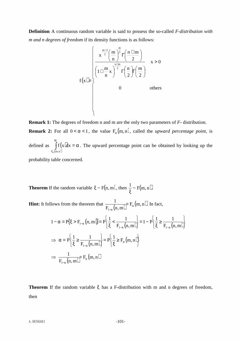
A.BENHARI -101-
Definition A continuous random variable is said to possess the so-called F-distribution with
m and n degrees of freedom if its density functions is as follows:
( )
>
Γ
Γ
+
+Γ
=
+
−
others0
0x
2
m
2
nx
n
m1
2
mn
n
mx
xf
2
mn
2
m
2
2m
Remark 1: The degrees of freedom n and m are the only two parameters of F- distribution.
Remark 2: For all 10 <α< , the value ( )n,mFα , called the upward percentage point, is
defined as ( )( )
α=∫+∞
α n,mF
dxxf . The upward percentage point can be obtained by looking up the
probability table concerned.
Theorem If the random variable ( )m,nF~ξ , then ( )n,mF~1
ξ.
Hint: It follows from the theorem that ( ) ( )n,mFm,nF
1
1α
α−
= . In fact,
( ) ( ) ( )
≥ξ
−=
<ξ
=>ξ=α−α−α−
α− m,nF
11P1
m,nF
11Pm,nFP1
111
⇒ ( ) ( )
≥
ξ=
≥ξ
=α αα−
n,mF1
Pm,nF
11P
1
⇒ ( ) ( )n,mFm,nF
1
1α
α−
=
Theorem If the random variable ξ has a F-distribution with m and n degrees of freedom,
then
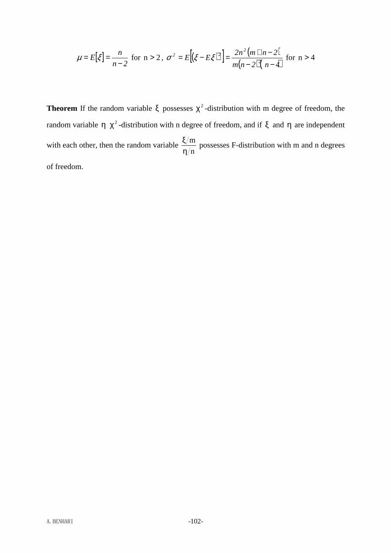
A.BENHARI -102-
[ ]2n
nE
−== ξµ for 2n > , ( )[ ] ( )
( ) ( )4n2nm
2nmn2EE
2
222
−−−+=−= ξξσ for 4n >
Theorem If the random variable ξ possesses 2χ -distribution with m degree of freedom, the
random variable η 2χ -distribution with n degree of freedom, and if ξ and η are independent
with each other, then the random variable n
m
ηξ
possesses F-distribution with m and n degrees
of freedom.
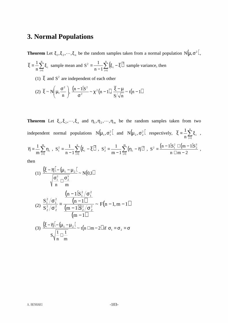
A.BENHARI -103-
3. Normal Populations
Theorem Let n21 ,,, ξξξ L be the random samples taken from a normal population ( )2,N σµ ,
∑=
ξ=ξn
1iin
1 sample mean and ( )∑
=
ξ−ξ−
=n
1i
2
i2
1n
1S sample variance, then
(1) ξ and 2S are independent of each other
(2)
σµξn
,N~2
, ( ) ( )1n~
S1n 22
2
−χσ−
, ( )1nt~nS
−µ−ξ
Theorem Let n21 ,,, ξξξ L and m21 ,,, ηηη L be the random samples taken from two
independent normal populations ( )211,N σµ and ( )2
22 ,N σµ respectively, ∑=
ξ=ξn
1iin
1,
∑=
η=ηm
1iim
1, ( )∑
=
ξ−ξ−
=n
1i
2
i21 1n
1S , ( )∑
=
η−η−
=m
1i
2i
22 1m
1S ,
( ) ( )2mn
S1mS1nS
32
212
−+−+−
= ,
then
(1) ( ) ( ) ( )1,0N~
mn
32
21
21
σ+
σ
µ−µ−η−ξ
(2)
( )( )
( )( )
( )1m,1nF~
1m
S1m1n
S1n
S
S22
22
21
21
22
22
21
21 −−
−σ−
−σ−
=σσ
(3) ( ) ( ) ( )2mnt~
m
1
n
1S
21 −++
µ−µ−η−ξ if σ=σ=σ 21
A.BENHARI -104-
Parameter Estimation

A.BENHARI -105-
1. Point Estimation
1.1. Point Estimators
Let n21 ,,, ξξξ L be the random samples taken from the same population characterized by a
random variable ξ , and θ an unknown parameter appearing in the distribution of ξ , by point
estimation we mean the attempt to look for a statistic ( )n21 ,,,g ξξξ L to estimate the unknown
parameter θ .
Unbiased Estimators An estimator ( )n21 ,,,g ξξξ L for a parameter θ is said to be unbiased
if ( )[ ] θ=ξξξθ n21 ,,,gE L .
Consistent Estimators An estimator ( )n21 ,,,g ξξξ L for a parameter θ is said to be
consistent if for all 0>ε , ( ) 0,,,gPlim n21n
=ε≥θ−ξξξθ+∞→L .
Mean Square Consistent Estimators An estimator ( )n21 ,,,g ξξξ L for a parameter θ is said
to be mean square consistent if ( )[ ] 0,,,gElim2
n21n
=θ−ξξξθ+∞→L .
Efficient Estimators A unbiased estimator ( )n211 ,,,g ξξξ L for a parameter θ is said to be
more efficient than another unbiased estimator ( )n212 ,,,g ξξξ L if
( )[ ] ( )[ ]2
n212
2
n211 ,,,gE,,,gE θ−ξξξ≤θ−ξξξ θθ LL
1.2. Method of Moments (MOM)
Assume that random samples n21 ,,, ξξξ L are taken from a population characterized by a
random variable ξ , if the distribution of population ξ has m unknown parameters
m21 ,,, θθθ L , let
A.BENHARI -106-
( ) [ ]k,,,
n
1i
ki m21
En
1 ξξ θθθ L=∑=
, m,,2,1k L=
This is a system of m equations with m unknowns, the solution to which is the so-called
MOM estimators of m21 ,,, θθθ L .
Remark: The method of moments is motivated by the following equation:
( ) ( ) [ ] ( ) [ ] ( ) [ ]k,,,
n
1i
k,,,
n
1i
ki,,,
n
1i
ki,,, m21m21m21m21
EEn
1E
n
1
n
1E ξξξξ θθθθθθθθθθθθ LLLL ===
∑∑∑
===
1.3. Maximum Likelihood Estimation (MLE)
Assume that random samples n21 ,,, ξξξ L are taken from the same population characterized
by a random variable ξ , if the distribution of population ξ has m unknown parameters
m21 ,,, θθθ L , one can define the likelihood function as follows:
if the random variable ξ is continuous and ( )( )xfmθθθ ,,, 21 L its probability density function,
then Likelihood function is defined as
( ) ( ) ( ) ( )∏=
θθθθθθ ξ=ξξξn
1ii,,,n21,,, m21m21
f,,,L LL L
if the random variable ξ is discrete and ( ) ( ) ( ) xPxpm21m21 ,,,,,, =ξ= θθθθθθ LL , then
Likelihood function is defined as
( ) ( ) ( ) ( )∏=
θθθθθθ ξ=ξξξn
1ii,,,n21,,, m21m21
p,,,L LL L
The MLE estimators ∗∗∗m21 ,θ,,θθ L are ones such that
( ) ( )( )n21,θ,,θθ,θ,,θθ
m21 ,ξ,,ξξLargmax,θ,,θθm21
m21
LL LL
=∗∗∗
Remark: It is clear that the resulting estimators ∗∗∗ θθθ m21 ,,, L are functions of n21 ,,, ξξξ L .
In practice, if the derivatives of a likelihood function ( )m21 ,,,L θθθ L with respect to the unknown
parameters exist, one can obtain the MLE estimator from the solution to the following
equations

A.BENHARI -107-
( )( )[ ]0
,,,ln 21,,, 21 =∂
∂
i
nmL
θξξξθθθ L
L , m,,2,1i L=

A.BENHARI -108-
2. Interval Estimation
Definition Let n21 ,,, ξξξ L be the random samples taken from the same population and θ an
unknown parameter appearing in the population distribution. If for all 10 <α< (usually
small enough), one can determine two statistics ( )n21 ,,,a ξξξα L and ( )n21 ,,,b ξξξα L such
that
( ) ( ) α−=ξξξ<θ<ξξξ αα 1,,,b,,,aP n21n21 LL
the interval ( ) ( )( )n21n21 ,,,b,,,,a ξξξξξξ αα LL is then called the confidence interval for the
unknown parameter θ , with the confidence coefficient α−1 .
Remark: In practice, one can consider one-tailed confidence interval:
( ) α−=ξξξ<θ<∞− α 1,,,bP n21 L or ( ) α−=+∞<θ<ξξξα 1,,,aP n21 L
Example Suppose n21 ,,, ξξξ L are the random samples taken from a normal population
( )2,N σµ .
(1) (Estimation of µ ) If the variance 2σ is known, it follows from ( )1,0N~nσµ−ξ
that for all
10 <α< ,
α−=
<σ
µ−ξα 1z
nP 2 ⇒ α−=
σ+ξ<µ<σ−ξ αα 1
nz
nzP 22
(2) (Estimation of µ ) If the variance 2σ is unknown, it follows from ( )1nt~nS
−µ−ξ that for
all 10 <α< ,
( ) α−=
−<µ−ξα 11nt
nSP 2 ⇒ ( ) ( ) α−=
−+ξ<µ<−−ξ αα 1
n
S1nt
n
S1ntP 22
(3) (Estimation of 2σ ) It follows from ( ) ( )1n~
S1n 22
2
−χσ−
that for all 10 <α< ,
( ) ( ) ( ) α−=
−χ<σ−<−χ αα− 11n
S1n1nP 2
22
22
21 ⇒ ( )
( )( )
( ) α−=
−χ−<σ<
−χ−
α−α
11n
S1n
1n
S1nP
221
22
22
2
Remark: 2zα , 2t α , ( )1n221 −χ α− and ( )1n2
2 −χα are the upward percentage points of the

A.BENHARI -109-
corresponding distributions.
Example Suppose the ransom samples n21 ,,, ξξξ L are taken from a normal population
( )211,N σµ , the random samples m21 ,,, ηηη L are taken from another normal population
( )222,N σµ and the two populations are independent with each other.
(1) ( )21ofEstimation µ−µ If the variances 21σ and 2
2σ are known, it follows from
( ) ( ) ( )1,0N~
mn
22
21
21
σ+σµ−µ−η−ξ
that for all 10 <α< ,
( ) ( ) α−=
<σ+σ
µ−µ−η−ξα 1z
mn
P 222
21
21
⇒ ( ) ( ) α−=
σ+σ+η−ξ<µ−µ<σ+σ−η−ξ αα 1
mnz
mnzP
22
21
221
22
21
2
(2) ( )21ofEstimation µ−µ If the variance 222
21 σ=σ=σ is unknown, it follows from
( ) ( ) ( )2mnt~
m
1
n
1S
21 −++
µ−µ−η−ξ, where
( ) ( )2mn
S1mS1nS
22
212
−+−+−= , that for all 10 <α< ,
( ) ( ) ( ) α−=
−+<+
µ−µ−η−ξα 12mnt
m
1
n
1S
P 221
⇒ ( ) ( ) ( ) ( ) ( ) α−=
+−++η−ξ<µ−µ<+−+−η−ξ αα 1m
1
n
1S2mnt
m
1
n
1S2mntP 2212
(3)
σσ
22
21ofEstimation It follows from
( ) ( )1n~S1n 2
21
21 −χ
σ−
and ( ) ( )1m~
S1m 222
22 −χ
σ−
that
( )( )
( )( )
( )1m,1nF~
1m
S1m1n
S1n
S
S22
22
21
21
22
22
21
21 −−
−σ−
−σ−
=σσ

A.BENHARI -110-
which leads to
( ) ( ) α−=
−−<σσ<−− αα− 11m,1nF
S
S1m,1nFP 22
222
21
21
21
⇒ ( ) ( ) α−=
−−<
σσ
<−− α−α
11m,1nF
1
S
S
1m,1nF
1
S
SP
2122
21
22
21
222
21

A.BENHARI -111-
Tests of Hypotheses
Statistical hypothesis 0H is an assumption about the unknown parameters appearing in a
population distribution or about the population distribution itself. A number of random
samples n21 ,,, ξξξ L taken from the population are then used to make the probability
trueisHrejectedisHP 00 as small as possible. This is realized in practice by setting up the
following equation:
α=trueisHrejectedisHP 00
Typically, 05.0=α , 01.0=α , or the like.
A.BENHARI -112-
1. Parameters from a Normal Population
Test of the hypothesis 00 :H µ=µ against the alternative 01 :H µ≠µ of the mean of a normal
distribution with known variance 2σ .
If the hypothesis 00 :H µ=µ is true, then ( )1,0N~n0
σµ−ξ
, which leads to
α=
≥σ
µ−ξ== α 2
00100 z
nPtrueisHacceptedisHPtrueisHrejectedisHP
⇒ if 20 z
nα<
σµ−ξ
, then 00 :H µ=µ , otherwise 01 :H µ≠µ
Test of the hypothesis 00 :H µ=µ against the alternative ( )001 :H µ>µµ<µ of the mean of
a normal distribution with known variance 2σ .
If the hypothesis 00 :H µ=µ is true, then ( )1,0N~n0
σµ−ξ
, which leads to
α=
>σ
µ−ξ=µ>µ=
α=
−<σ
µ−ξ=µ<µ=
α
α
zn
PtrueisHacceptedis:HPtrueisHrejectedisHP
zn
PtrueisHacceptedis:HPtrueisHrejectedisHP
000100
000100
⇒
µ>µµ=µ≤σ
µ−ξ
µ<µµ=µ−≥σ
µ−ξ
α
α
01000
01000
:Hotherwise,:Hthen,zn
if
:Hotherwise,:Hthen,zn
if
Test of the hypothesis 00 :H µ=µ against the alternative 01 :H µ≠µ of the mean of a normal
distribution with unknown variance.
If the hypothesis 00 :H µ=µ is true, then ( )1nt~nS
0 −µ−ξ
, which leads to
A.BENHARI -113-
( ) α=
−≥µ−ξ
== α 1ntnS
PtrueisHacceptedisHPtrueisHrejectedisHP 20
0100
⇒ ( ) 010020 :Hotherwise,:Hthen,1nt
nSif µ≠µµ=µ−<
µ−ξα
Test of the hypothesis 00 :H µ=µ against the alternative ( )001 :H µ>µµ<µ of the mean of
a normal distribution with unknown variance.
If the hypothesis 00 :H µ=µ is true, then ( )1nt~nS
0 −µ−ξ
, which leads to
( )
( )
α=
−>µ−ξ
=µ>µ=
α=
−−<µ−ξ
=µ<µ=
α
α
1ntnS
PtrueisHacceptedis:HPtrueisHrejectedisHP
1ntnS
PtrueisHacceptedis:HPtrueisHrejectedisHP
000100
000100
⇒
( )
( )
µ>µµ=µ−≤µ−ξ
µ<µµ=µ−−≥µ−ξ
α
α
01000
01000
:Hotherwise,:Hthen,1ntnS
if
:Hotherwise,:Hthen,1ntnS
if
Test of the hypothesis 00 :H σ=σ against the alternative 01 :H σ≠σ of the variance of a
normal distribution.
If the hypothesis 00 :H σ=σ is true, then ( ) ( )1n~
S1n 220
2
−χσ−
, which leads to
( ) ( ) ( ) ( ) α=
−χ≥
σ−
−χ<
σ−= αα− 1n
S1n1n
S1nPtrueisHrejectedisHP 22
0
2
2120
2
00 U
⇒ ( ) ( ) ( ) 1o220
2
21 Hotherwise,Hthne,1nS1n
1nif −χ<σ−≤−χ αα−
Test of the hypothesis 00 :H σ=σ against the alternative ( )001 :H σ>σσ<σ of the variance
of a normal distribution.
A.BENHARI -114-
If the hypothesis 00 :H σ=σ is true, then ( ) ( )1n~
S1n 220
2
−χσ−
, which leads to
( ) ( )
( ) ( )
α=
−χ<σ−=σ<σ
α=
−χ>σ−=σ>σ
=
α−
α
1nS1n
PtrueisHacceptedis:HP
1nS1n
PtrueisHacceptedis:HP
trueisHrejectedisHP
120
2
001
20
2
001
00
⇒
( ) ( )( ) ( )
σ<σσ=σ−χ>σ−
σ>σσ=σ−χ<σ−
α−
α
0100120
2
010020
2
:Hotherwise,:Hthen,1nS1n
if
:Hotherwise,:Hthen,1nS1n
if
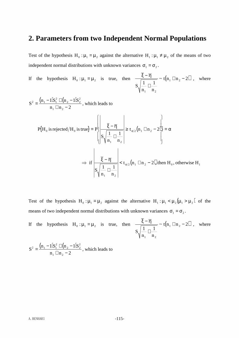
A.BENHARI -115-
2. Parameters from two Independent Normal Populations
Test of the hypothesis 210 :H µ=µ against the alternative 211 :H µ≠µ of the means of two
independent normal distributions with unknown variances 21 σ=σ .
If the hypothesis 210 :H µ=µ is true, then ( )2nnt~
n
1
n
1S
21
21
−++
η−ξ, where
( ) ( )2nn
S1nS1nS
21
222
2112
−+−+−
= , which leads to
( ) α=
−+≥+
η−ξ= α 2nnt
n
1
n
1S
PtrueisHrejectedisHP 212
21
00
⇒ ( ) 10212
21
Hotherwise,Hthen,2nnt
n
1
n
1S
if −+<+
η−ξα
Test of the hypothesis 210 :H µ=µ against the alternative ( )21211 :H µ>µµ<µ of the
means of two independent normal distributions with unknown variances 21 σ=σ .
If the hypothesis 210 :H µ=µ is true, then ( )2nnt~
n
1
n
1S
21
21
−++
η−ξ, where
( ) ( )2nn
S1nS1nS
21
222
2112
−+−+−
= , which leads to
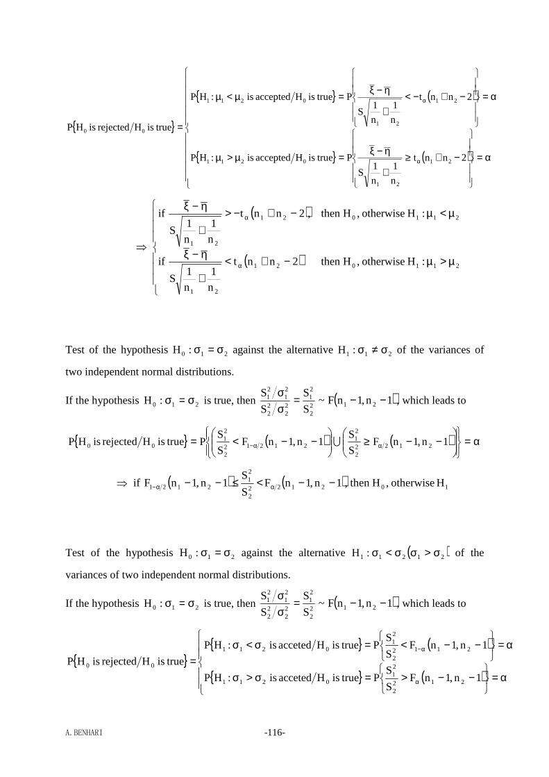
A.BENHARI -116-
( )
( )
α=
−+≥+
η−ξ=µ>µ
α=
−+−<+
η−ξ=µ<µ
=
α
α
2nnt
n
1
n
1S
PtrueisHacceptedis:HP
2nnt
n
1
n
1S
PtrueisHacceptedis:HP
trueisHrejectedisHP
21
21
0211
21
21
0211
00
⇒
( )
( )
µ>µ−+<+
η−ξ
µ<µ−+−>+
η−ξ
α
α
211021
21
211021
21
:Hotherwise,Hthen2nnt
n
1
n
1S
if
:Hotherwise,Hthen,2nnt
n
1
n
1S
if
Test of the hypothesis 210 :H σ=σ against the alternative 211 :H σ≠σ of the variances of
two independent normal distributions.
If the hypothesis 210 :H σ=σ is true, then ( )1n,1nF~S
S
S
S212
2
21
22
22
21
21 −−=
σσ
, which leads to
( ) ( ) α=
−−≥
−−<= αα− 1n,1nF
S
S1n,1nF
S
SPtrueisHrejectedisHP 2122
2
21
212122
21
00 U
⇒ ( ) ( ) 1021222
21
2121 Hotherwise,Hthen,1n,1nFS
S1n,1nFif −−<≤−− αα−
Test of the hypothesis 210 :H σ=σ against the alternative ( )21211 :H σ>σσ<σ of the
variances of two independent normal distributions.
If the hypothesis 210 :H σ=σ is true, then ( )1n,1nF~S
S
S
S212
2
21
22
22
21
21 −−=
σσ
, which leads to
( )
( )
α=
−−>=σ>σ
α=
−−<=σ<σ=
α
α−
1n,1nFS
SPtrueisHaccetedis:HP
1n,1nFS
SPtrueisHaccetedis:HP
trueisHrejectedisHP
2122
21
0211
21122
21
0211
00
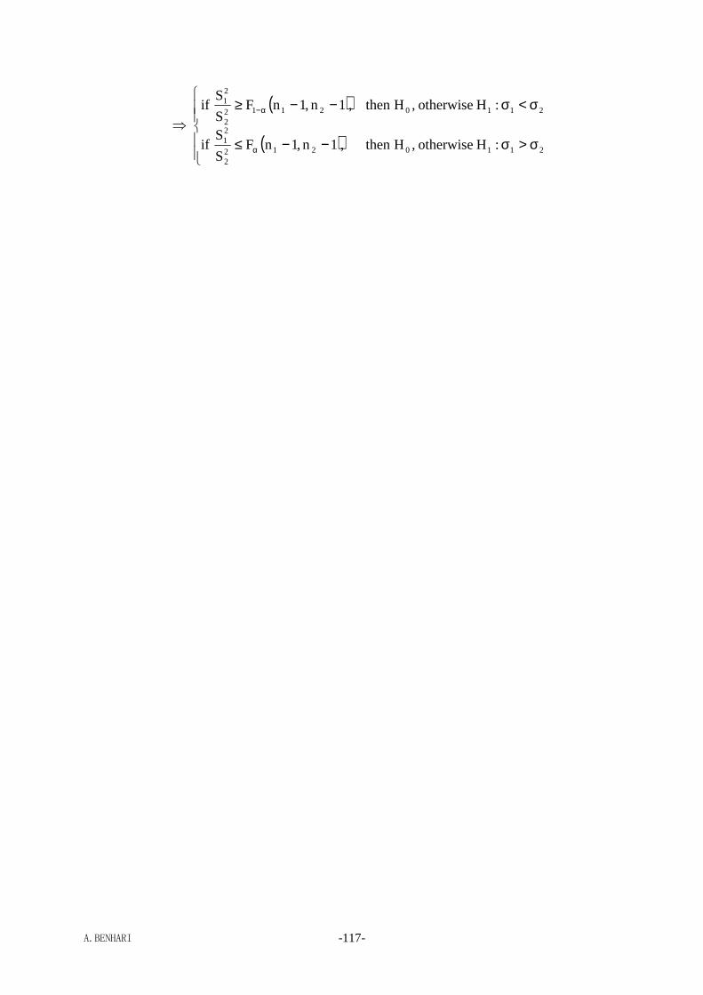
A.BENHARI -117-
⇒
( )
( )
σ>σ−−≤
σ<σ−−≥
α
α−
21102122
21
211021122
21
:Hotherwise,Hthen,1n,1nFS
Sif
:Hotherwise,Hthen,1n,1nFS
Sif

A.BENHARI -118-
III. RANDOM PTOCESSES

A.BENHARI -119-
Introduction
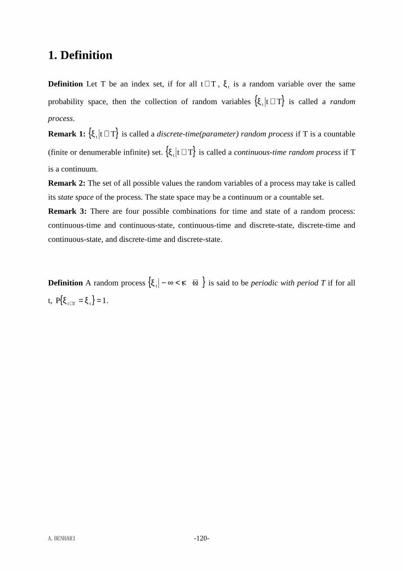
A.BENHARI -120-
1. Definition
Definition Let T be an index set, if for all Tt ∈ , tξ is a random variable over the same
probability space, then the collection of random variables Ttt ∈ξ is called a random
process.
Remark 1: Ttt ∈ξ is called a discrete-time(parameter) random process if T is a countable
(finite or denumerable infinite) set. Ttt ∈ξ is called a continuous-time random process if T
is a continuum.
Remark 2: The set of all possible values the random variables of a process may take is called
its state space of the process. The state space may be a continuum or a countable set.
Remark 3: There are four possible combinations for time and state of a random process:
continuous-time and continuous-state, continuous-time and discrete-state, discrete-time and
continuous-state, and discrete-time and discrete-state.
Definition A random process +∞<<∞−ξ tt is said to be periodic with period T if for all
t, 1P tTt =ξ=ξ + .
A.BENHARI -121-
2. Family of Finite-Dimensional Distributions
A random process Ttt ∈ξ is often characterized by the joint distributions of every possible
collection of finite random variables n21 ttt ,,, ξξξ L taken from the process:
( ) nt2t1tnn2211 x;;x;xPt,x;;t,x;t,xFn21
<ξ<ξ<ξ= LL
All these joint distributions constitute the family of finite-dimensional distributions of the
process.
The Properties of the family of finite-Dimensional Distributions:
(1) Symmetry
( ) ( ) ( ) ( ) ( ) ( ) ( )( )nQnQ2Q2Q1Q1Qnn2211 t,x;;t,x;t,xFt,x;;t,x;t,xF LL =
where ( ) ( ) ( )( )nQ,,2Q,1Q L is a permutation of ( )n,,2,1 L .
(2) Consistency
( ) ( )mnmn1n1nnn2211nn2211 t,x;;t,x;t,x;;t,x;t,xFt,x;;t,x;t,xF ++++ +∞=+∞== LLL
Kolmogorov Theorem If a family of finite-dimensional distributions satisfies the symmetry
and consistency described above, there must be then a random process such that the family is
its family of finite-dimensional distributions.
Two random processes Ttt ∈ξ and Ttt ′∈′η ′ are jointly characterized by the joint
distributions of every possible collection of finite random variables taken from the two
processes respectively
( ) mt1tnt1tmm11nn11 y;;y;x;;xPt,y;;t,y;t,x;;t,xFm1n1
<η<η<ξ<ξ=′′ ′′ξη LLLL
Two random processes Ttt ∈ξ and Ttt ′∈′η ′ are said to be independent if
( ) ( ) ( )mm11nn11mm11nn11 t,y;;t,yFt,x;;t,xFt,y;;t,y;t,x;;t,xF ′′=′′ ηξξη LLLL
A.BENHARI -122-
3. Mathematical Expectations
Definition Let Ttt ∈ξ be a random process, then
• The mean value of the process is defined as
[ ]tt E ξ=µ .
• The variance of the process is defined as
[ ] [ ] 2t
2t
2
tt2t EE µ−ξ=µ−ξ=σ
• The correlation function of the process is defined as
( ) [ ]21 tt21 Et,tR ξξ=
• The covariance of the process is defined as
( ) ( )( )[ ] ( )212211 tt21tttt21 t,tREt,tcov µµ−=µ−ξµ−ξ=
Definition A random processes Ttt ∈ξ is said to be weakly stationary if for all Tt ∈ and
Tt ∈τ+ , [ ] ( )τ=ξξ τ+ RE tt , i.e., [ ]τ+ξξ ttE is independent of the choice of t.
Definition Two random processes ξ∈ξ Ttt and η∈η Ttt are said to be uncorrelated if for
all ξ∈ Tt1 and η∈ Tt 2 , ( ) [ ] 0Et,tR21 tt21 =ξη=ξη .
A.BENHARI -123-
4. Examples
4.1. Processes with Independent, Stationary or Orthogonal
Increments
Definition (Independent Increments) A random process Ttt ∈ξ is said to have
independent increments if for all Tttt n21 ∈<<< L , the increments
1nn2312 tttttt ,,,−
ξ−ξξ−ξξ−ξ L are independent of each other.
Example Let +∞<≤ξ tat be a random process with independent increments and
1.ConstP a ==ξ , then for all 21 tta <≤ , ( ) 2t21 1
t,tcov σ= .
Proof:
For all +∞<≤ ta , let [ ]ttt E ξ−ξ=η , then the process +∞<≤η tat is one with
independent increments, mean zero and 10P a ==η . Thus we have
( ) ( )( )[ ] [ ] ( )[ ]1112121122 tttttttttt12 EEEEEt,tcov ηη+η−η=ηη=ξ−ξξ−ξ=
( )[ ] 2t
2
tt
2
tttt 1111112EEEE σ=
ξ−ξ=
η+ηη−η= #
Remark: ( ) 2
t,tmin21 21t,tcov σ=
Definition (Stationary Increments) A random process Ttt ∈ξ is said to have stationary
increments if for all Ttt ∈τ+< , the distribution of increment tt ξ−ξ τ+ has nothing to do
with t.
Definition (Orthogonal Increments) A zero-mean random process Ttt ∈ξ is said to have
orthogonal increments if for all Ttttt 4321 ∈<≤< , ( )( )[ ] 0E3412 tttt =ξ−ξξ−ξ .
Remark: ξ and η are said to be orthogonal if [ ] 0E =ηξ
A.BENHARI -124-
4.2. Normal Processes
Definition A random process Ttt ∈ξ is said to be a normal/Gaussian process if all its
finite-dimensional distributions are normal/Gaussian.

A.BENHARI -125-
Markov Processes (1)
A.BENHARI -126-
1. General Properties
Definition A random process Ttt ∈ξ is called a Markov process if for all
Ttttt 1kk21 ∈<<<< +L , its conditional distributions satisfy
( ) =−−++ξξξ + 111k1kkk1k1k t,x;;t,x;t,xt,xF1tkt1kt
LL
kt1kt1t1ktkt1kt xxPx;;x;xxPk1k11kk1k
=ξ<ξ==ξ=ξ=ξ<ξ= +−+ +−+L
( )kk1k1k t,xt,xFkt1kt ++ξξ +
=
Remark 1: The definition of a Markov process means that the future is only dependent on the
present and has nothing to do with the past (History can tell nothing about future).
Remark 2: A Markov process is called a Markov chain if its state space is discrete.
Definition A Markov process Ttt ∈ξ is said to be homogenous if for all Ttt ∈τ+< , the
conditional distribution ( ) xyPt,xt,yF tt =ξ<ξ=τ+ τ+ is independent of time t, i.e.,
( ) ( )x,yFt,xt,yF τ=τ+ .
Theorem Let 0tt ≥ξ be an IID random process, i.e., for all τ+<<<<≤ kk21 tttt0 L , the
random variables τ+ξξξξkk21 tttt ,,,, L are independent and identically distributed, then the
process is a homogenous Markov process.
Proof:
1tkt
1tktt
1tktt x;;xP
x;;x;xPx;;xxP
1k
1kk
1kk =ξ=ξ=ξ=ξ<ξ
==ξ=ξ<ξ τ+τ+
L
LL
xP
xPxP
xPxPxPk
1k
1kk
t1tkt
1tktt
tindependen<ξ=
=ξ=ξ=ξ=ξ<ξ
= τ+τ+
L
L
ktt
kt
ktt
tindependenkt
kttxxP
xP
x;xP
xP
xPxPkk
k
kk
k
kk =ξ<ξ==ξ
=ξ<ξ=
=ξ=ξ<ξ
= τ+τ+τ+
This shows that the process is a Markov Process. Furthermore, for all τ+<≤ tt0 ,
yxPxPxPyxP 0ddistributeyidenticall
ttindependen
tt =ξ<ξ=<ξ=<ξ==ξ<ξ τττ+τ+
This shows that the Markov process is homogenous. #

A.BENHARI -127-
Remark: From the proof of the theorem, one can see
Independence ⇒ Markov; Identical distribution ⇒ Homogeneity
Theorem Let 0tt ≥ξ be a random process with 00 =ξ .
(1) If the increments of 0tt ≥ξ are independent, the process is a Markov process.
(2) If the increments of 0tt ≥ξ are both independent and stationary, then the process is a
homogenous Markov process.
Proof:
1t2tkt
1t2tktt
1t2tktt x;x;;xP
x;x;;x;xPx;x;;xxP
12k
12kk
12kk =ξ=ξ=ξ=ξ=ξ=ξ<ξ
==ξ=ξ=ξ<ξ τ+τ+
L
LL
1t12tt1kktt
1t12tt1kkttktt
x;xx;;xxP
x;xx;;xx;xxP
1121kk
1121kkkk
=ξ−=ξ−ξ−=ξ−ξ=ξ−=ξ−ξ−=ξ−ξ−<ξ−ξ
=−
−τ+
−
−
L
L
1t12tt1kktt
1t12tt1kkttktt
incrementtindependen xPxxPxxP
xPxxPxxPxxP
1121kk
1121kkkk
=ξ−=ξ−ξ−=ξ−ξ=ξ−=ξ−ξ−=ξ−ξ−<ξ−ξ
=−
−τ+
−
−
L
L
kt
ktktt
ktt xP
x;xxPxxP
k
kkk
kk =ξ=ξ−<ξ−ξ
=−<ξ−ξ= τ+τ+
ktt
kt
kttxxP
xP
x;xPkk
k
kk =ξ<ξ==ξ
=ξ<ξ= τ+
τ+
This shows that the process is a Markov Process. Furthermore, for all 0t ≥ ,
kttincrementsstationary
kttktt xxPxxPxxPkkkk
−<ξ−ξ=−<ξ−ξ==ξ<ξ τ+τ+τ+
kt
ktktt
incrementstindependenkt
ktktt
xP
x;xxP
xP
xPxxP
=ξ=ξ−<ξ−ξ
==ξ
=ξ−<ξ−ξ= τ+τ+
ktt
kt
ktt xxPxP
x;xP=ξ<ξ=
=ξ=ξ<ξ
= τ+τ+
This shows that the Markov process is homogenous. #
Remark: In the probability space ( )P,,ΠΩ , we have
( ) ( ) ( ) ( ) ( ) y,yx,y,x, =ωη−=ωη−ωξΩ∈ωω==ωη=ωξΩ∈ωω
A.BENHARI -128-
2. Discrete-Time Markov Chains
For a discrete-time Markov chain, the conditional probability xyP nmn =ξ=ξ + is often
called its m-step transition probability.
Definition A discrete-time Markov chain Tnn ∈ξ is said to be homogenous if its transition
probability xyP nmn =ξ=ξ + is independent of n.
Remark: From now on, discrete-time Markov chains appearing in this section are all
assumed to be homogenous.
2.1. Transition Probabilities
For a homogenous Markov chain, its k-step transition probability is often denoted as
( ) xyPp nknk
xy =ξ=ξ= + , where k is a non-negative integer. Note that
( )
≠=
==ξ=ξ=yx0
yx1xyPp nn
0xy .
Chapman-Kolmogorov Theorem Let L,1,0nn =ξ be a homogenous Markov chain, then
( ) ( ) ( )∑=+
z
kzy
nxz
knxy ppp
Proof:
( )
∑ =ξ
=ξ=ξ=ξ=
=ξ=ξ=ξ
==ξ=ξ= +++++++
+
z m
mmkmkn
m
mmknmmkn
knxy xP
x;z;yP
xP
x;yPxyPp
∑ =ξ
=ξ=ξ=ξ=ξ=ξ= ++++
z m
mmkmmkmkn
xP
x;zPx;zyP
∑ =ξ=ξ=ξ=ξ= ++++z
mmkmkmkn xzPzyP ( ) ( )∑=z
nzy
kxz pp #
Remark: From the Chapman-Kolmogorov theorem, one can conclude that k-step transition
probabilities can be derived from the one-step transition probabilities. In fact,
( ) ∑=z
zyxz2
xy ppp , ( ) ( )∑=z
zy2
xz3
xy ppp , , ( ) ( )∑ −=z
zy1k
xzk
xy ppp ,
A.BENHARI -129-
Example If let
=
MMMMM
LL
MMMMM
LL
LL
nn1n0n
n11110
n00100
ppp
ppp
ppp
P , ( )
( ) ( ) ( )
( ) ( ) ( )
( ) ( ) ( )
=
MMMMM
LL
MMMMM
LL
LL
mnn
m1n
m0n
mn1
m11
m10
mn0
m01
m00
m
ppp
ppp
ppp
P
be the one-step transition matrix and m-step transition matrix of the chain, respectively, then
the theorem can be expressed in matrix form
( ) mm PP =
In fact, from Chapman-Kolmogorov theorem we have
( ) ∑∑+∞
=
==0z
zyxzz
zyxz2
xy ppppp ⇒ ( ) 22 PP =
( ) ( ) ( )∑∑+∞
=
==0z
zy2
xzz
zy2
xz3
xy ppppp ⇒ ( ) ( ) 323 PPPP ==
……
In this way we obtain that
( ) mm PP =
Theorem Let L,1,0nn =ξ be a homogenous Markov chain, then the distribution of nξ can
be expressed as
( ) ( )∑∑∑ ==ξ=ξ=ξ==ξ=ξ==ξ=y
nyxy
y00n
y0nn
nx ppyPyxPy;xPxPp
where yPp 0y =ξ= is the initial probability.
Remark 1: Recall that k-step transition probabilities can be derived from one-step transition
probabilities, the theorem shows that the distribution of nξ can be determined only by one-
step transition probabilities as well as initial probabilities.
Remark 2: If let
( )LL ,p,,p,p k10=p , ( ) ( ) ( ) ( )( )LL ,p,,p,p nk
n1
n0
n =p
be the initial probability vector and the probability vector at the n moment, respectively, then
the theorem can be expressed in matrix form
A.BENHARI -130-
( ) ( ) nnn PP ppp ==
Theorem Let L,1,0nn =ξ be a homogenous Markov chain, then the joint distribution of
1kk21 nnnn ,,,,+
ξξξξ L can be expressed as
==ξ=ξ=ξ ++ 1nkn1kn x;;x;xP1k1k
L
1nkn1nkn1kn x;;xPx;;xxP1k1k1k
=ξ=ξ=ξ=ξ=ξ= ++LL
1nknkn1kn x;;xPxxP1kk1k
=ξ=ξ=ξ=ξ= ++L
( ) 1nknnn
xx x;;xPp1k
k1k
1kk=ξ=ξ= −+
+L
( ) ( ) ( )k1k
1kk
1kk
k1k
12
211
nnxx
nnxx
nnxx1n pppxP −−− +
+
−
−=ξ= L
Remark: Again, the joint distribution of 1kk21 nnnn ,,,,
+ξξξξ L can be determined by one-step
transition probabilities as well as initial probabilities.
2.2. Classification of States
2.2.1. Communication
Definition A state y is said to be accessible from a state x if there is a nonnegative integer n
such that ( ) 0p nxy > , often denoted by yx → . Two states x and y are said to communicate with
each other if they are accessible from one another, often denoted by yx ↔ .
Theorem Communication is an equivalence relation, i.e.,
(1) (Reflexivity) for all states x, xx ↔
(2) (Symmetry) for any two states x and y, if yx ↔ , then xy ↔
(3) (Transitivity) for any three states x, y and z, if yx ↔ and zy ↔ , then zx ↔
Hint:
( ) 01
xP
x;xPxxPp
0
0000
0xx >=
=ξ=ξ=ξ
==ξ=ξ= (Reflexivity)
( )
( ) xy0pxy
0pyxyx k
yx
nxy ↔⇒
>⇒→>⇒→
⇒↔ (Symmetry)
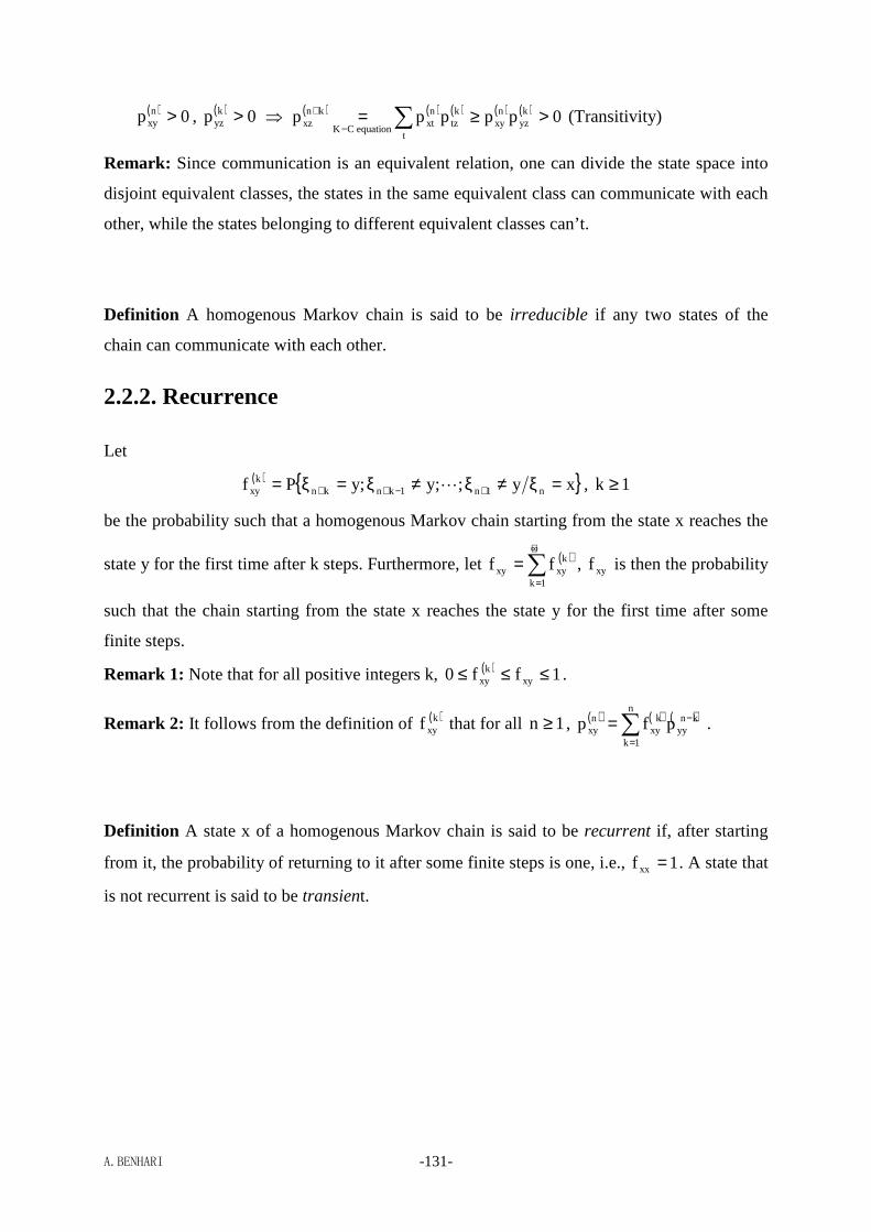
A.BENHARI -131-
( ) 0p nxy > , ( ) 0p k
yz > ⇒ ( ) ( ) ( ) ( ) ( ) 0ppppp kyz
nxy
t
ktz
nxt
equationCK
knxz >≥= ∑−
+ (Transitivity)
Remark: Since communication is an equivalent relation, one can divide the state space into
disjoint equivalent classes, the states in the same equivalent class can communicate with each
other, while the states belonging to different equivalent classes can’t.
Definition A homogenous Markov chain is said to be irreducible if any two states of the
chain can communicate with each other.
2.2.2. Recurrence
Let
( ) xy;;y;yPf n1n1knknk
xy =ξ≠ξ≠ξ=ξ= +−++ L , 1k ≥
be the probability such that a homogenous Markov chain starting from the state x reaches the
state y for the first time after k steps. Furthermore, let ( )∑+∞
=
=1k
kxyxy ff , xyf is then the probability
such that the chain starting from the state x reaches the state y for the first time after some
finite steps.
Remark 1: Note that for all positive integers k, ( ) 1ff0 xyk
xy ≤≤≤ .
Remark 2: It follows from the definition of ( )kxyf that for all 1n ≥ , ( ) ( ) ( )∑
=
−=n
1k
knyy
kxy
nxy pfp .
Definition A state x of a homogenous Markov chain is said to be recurrent if, after starting
from it, the probability of returning to it after some finite steps is one, i.e., 1f xx = . A state that
is not recurrent is said to be transient.

A.BENHARI -132-
Example Let
→
→
→
→
=
↓↓↓↓
1000
41
41
41
41
0021
21
0021
21
d
c
b
a
dcba
P be the one-step transition probability matrix of
a Markov chain, then the states a, b and d are recurrent, while c is transient..
Theorem A state x of a homogenous Markov chain is recurrent if and only if ( ) +∞=∑+∞
=1n
nxxp .
Proof:
( ) ( ) ( ) ( ) ( ) ( ) ( )∑ ∑∑∑∑∑∑=
−
== =
−
= =
−
=
===N
1k
kN
0t
txx
kxx
N
1k
N
kn
knxx
kxx
N
1n
n
1k
knxx
kxx
N
1n
nxx pfpfpfp
(1) Suppose ( ) +∞=∑+∞
=1n
nxxp , then
( ) ( ) ( ) ( ) ( )∑ ∑∑ ∑∑= ==
−
==
≤=N
1k
N
0t
txx
kxx
N
1k
kN
0t
txx
kxx
N
1n
nxx pfpfp ⇒
( )
( )
( )
( )
( )∑∑
∑
∑
∑
=
=
=
=
= ≤+
=N
1k
kxxN
1t
txx
N
1n
nxx
N
0t
txx
N
1n
nxx
fp1
p
p
p
⇒
( )
( ) ( )
( ) 1ff1p1
plim xx
1k
kxx
pbecauseN
1t
txx
N
1n
nxx
N1n
nxx
≤=≤=+
∑∑
∑ ∞+
=+∞=∑
=
=
+∞→ ∞+
=
⇒ 1f xx =
This implies that x is a recurrent state.
(2) Suppose 1f xx = , we now prove that ( ) +∞=∑+∞
=1n
nxxp . By reduction to absurdity, we first
assume that ( ) +∞<∑+∞
=1n
nxxp . Then, for all NN1 ≤′≤ ,
( ) ( ) ( ) ( ) ( )∑ ∑∑ ∑∑′
=
′−
==
−
==
≥=N
1k
NN
0t
txx
kxx
N
1k
kN
0t
txx
kxx
N
1n
nxx pfpfp ⇒ ( )
( )
( )∑
∑∑ ′−
=
=′
= +≤
NN
1t
txx
N
1n
nxxN
1k
kxx
p1
pf
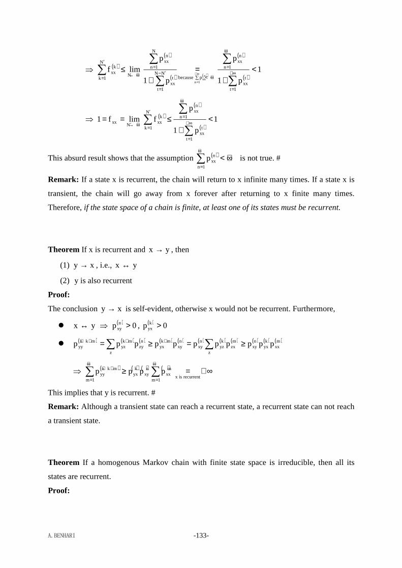
A.BENHARI -133-
⇒ ( )
( )
( ) ( )
( )
( )1
p1
p
p1
plimf
1t
txx
1n
nxx
pbecauseNN
1t
txx
N
1n
nxx
N
N
1k
kxx
1n
nxx
<+
=+
≤∑
∑
∑
∑∑ ∞+
=
+∞
=
+∞<∑′−
=
=
+∞→
′
=∞+
=
⇒ ( )
( )
( )1
p1
pflimf1
1t
txx
1n
nxxN
1k
kxx
Nxx <
+≤==
∑
∑∑ ∞+
=
+∞
=′
=+∞→′
This absurd result shows that the assumption ( ) +∞<∑+∞
=1n
nxxp is not true. #
Remark: If a state x is recurrent, the chain will return to x infinite many times. If a state x is
transient, the chain will go away from x forever after returning to x finite many times.
Therefore, if the state space of a chain is finite, at least one of its states must be recurrent.
Theorem If x is recurrent and yx → , then
(1) xy → , i.e., yx ↔
(2) y is also recurrent
Proof:
The conclusion xy → is self-evident, otherwise x would not be recurrent. Furthermore,
yx ↔ ⇒ ( ) 0p nxy > , ( ) 0p k
yx >
( ) ( ) ( ) ( ) ( ) ( ) ( ) ( ) ( ) ( ) ( )mxx
kyx
nxy
z
mzx
kyz
nxy
nxy
mkyx
z
nzy
mkyz
mknyy ppppppppppp ≥=≥= ∑∑ ++++
⇒ ( ) ( ) ( ) ( ) ∞+=≥ ∑∑+∞
=
+∞
=
++
recurrentisx1m
mxx
nxy
kyx
1m
mknyy pppp
This implies that y is recurrent. #
Remark: Although a transient state can reach a recurrent state, a recurrent state can not reach
a transient state.
Theorem If a homogenous Markov chain with finite state space is irreducible, then all its
states are recurrent.
Proof:
A.BENHARI -134-
Recall that a homogenous Markov chain with finite state space must have at least a recurrent
state x. For all other states y, it follows from the irreducibility of the chain that x and y are
communicate with each other and therefore y must also be recurrence. #
2.2.3. Decomposition of a State Space
Definition Let S be the state space of a homogenous Markov chain and SA ⊆ , A is said to be
closed if the states in A can not reach the states outside A, i.e., for all Ax ∈ , Ay ∉ and
1n ≥ , ( ) 0p nxy = .
Remark: The fact that A is closed does not exclude the possibility of a state outside A
reaching a state inside A.
Theorem Let R be the set of all recurrent states of a homogenous Markov chain, then
(1) R is closed.
(2) If a binary relation ~ is defined on R such that for all Ry,x ∈ , yxy~x def ↔= ,
then the relation is an equivalent relation.
Hint: As we have proven in the preceding subsection, a recurrent state can’t reach a transient
state. Thus R is closed.
Remark 1: Since the communication relation ~ in R is an equivalent relation, R can be then
divided into disjoint equivalent classes L++= 21 RRR . It is clear that each of equivalent
classes is also closed.
Remark 2: The state space S of a homogenous Markov chain can be decomposed as
L+++=+= 21 RRTRTS
where T is the set of all transient states of the chain.
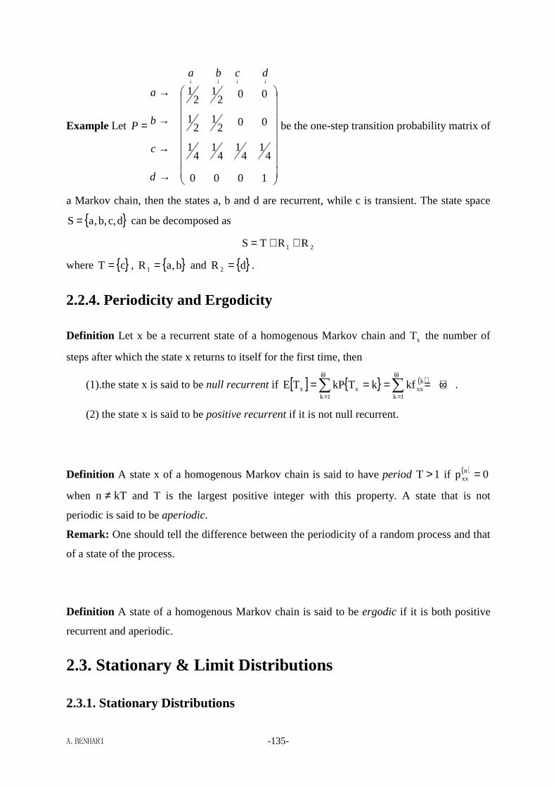
A.BENHARI -135-
Example Let
→
→
→
→
=
↓↓↓↓
1000
41
41
41
41
0021
21
0021
21
d
c
b
a
dcba
P be the one-step transition probability matrix of
a Markov chain, then the states a, b and d are recurrent, while c is transient. The state space
d,c,b,aS= can be decomposed as
21 RRTS ++=
where cT = , b,aR1 = and dR2 = .
2.2.4. Periodicity and Ergodicity
Definition Let x be a recurrent state of a homogenous Markov chain and xT the number of
steps after which the state x returns to itself for the first time, then
(1).the state x is said to be null recurrent if [ ] ( ) +∞==== ∑∑+∞
=
+∞
= 1k
kxx
1kxx kfkTkPTE .
(2) the state x is said to be positive recurrent if it is not null recurrent.
Definition A state x of a homogenous Markov chain is said to have period 1T > if ( ) 0p nxx =
when kTn ≠ and T is the largest positive integer with this property. A state that is not
periodic is said to be aperiodic.
Remark: One should tell the difference between the periodicity of a random process and that
of a state of the process.
Definition A state of a homogenous Markov chain is said to be ergodic if it is both positive
recurrent and aperiodic.
2.3. Stationary & Limit Distributions
2.3.1. Stationary Distributions

A.BENHARI -136-
Definition Let ijp be the one-step transition probability of a homogenous Markov chain, a
discrete distribution iπ is called the stationary distribution of the chain if i ij ji
pπ π=∑ .
Remark: if i 0π ≥ and ii
1π =∑ , then iπ is said to be a discrete distribution.
2.3.2. Limit Distributions
Definition A homogenous Markov chain is said to be ergodic if ( ) 0plim yn
xyn
≥π=+∞→
and
1y
y =π∑ .
Remark 1: yπ are often said to be the chain’s limit distribution.
Remark 2: ( )y
nxy
nplim π=
+∞→ means that ( )n
xyp is independent of the starting state x when n is
large enough.
2.3.3. The relation between Stationary Distributions and Limit
Distributions
Definition A homogenous Markov chain is said to be regular if there is a positive integer n
such that for all states x and y of the chain, ( ) 0p nxy > .
Remark: If the state space is finite, regular and irreducible are the same things, if the state
space is infinite, regular must lead to irreducible, but irreducible dose not necessarily lead to
regular.
Theorem (Ergodic Theorem) If a finite-state homogenous Markov chain is regular, then the
chain is ergodic and its limit distribution is also its stationary distribution.
2.4. Examples: Simple Random Walks
By the simple random walk of a particle on a line, one means that at each moment, the
particle moves its location either one step forwards with probability p or one step backwards
with probability p1q −= .
A.BENHARI -137-
Let L,1,0nn =ξ be a random process such that nξ indicates the location of the particle at
the moment n, we will then address the following issues:
Is the process a homogeneous Markov chain?
Let LL ,,,, m21 τττ be the random variables such that 1m =τ indicates the event that
the particle moves one step forwards at the moment m and 1m −=τ the event that the
particle moves one step backwards at the moment m, then 0
n
1mmn k+τ=ξ ∑
=
, where 0k is
the initial location of the particle. Note that LL ,,,, m21 τττ are independent and
identically distributed with ( )
−==−=
==τ1kqp1
1kpkP m for all m. It can be then
easily proven that the process L,1,0nn =ξ is one with independent and stationary
increments and therefore a homogenous Markov chain.
?kP n ==ξ
2
kkn
2
kknn
2
kkn0
n
1m
m0
n
1mmn
00
0qpC
2
kkn
2
1PkkPkP
+−−+
−+==
=
−+
=
+τ=
=+τ==ξ ∑∑
?ijP n1n ==ξ=ξ +
−=+=
==ξ=ξ +
others0
1ijq
1ijp
ijP n1n , 0n ≥ .
A.BENHARI -138-
Appendix Eigenvalue Diagonalization
Definition Let A be a nn × matrix, if there is a nonzero number λ and a nonzero vector x
such that xx λ=A , then λ is called an eigenvalue of A and x an eigenvector with respect to
λ .
Remark:
xx λ=A ⇒ ( ) 0x =λ− IA ⇒ 0IA =λ−
There are at most n different eigenvalues for a nn × matrix.
Theorem If a nn × matrix A has n linearly-independent eigenvectors n21 ,,, xxx L , then A
can be diagonalized as
( )n211 ,,,diagAXX λλλ=Λ=−
L
where ( )n21 ,,,X xxx L= .
Remark:
Λ= XAX ⇒ 1XXA −Λ= ⇒ 1nn XXA −Λ=
Example Let
−−
=b1b
aa1A , where 1b,a0 << .
(1) The eigenvalues and eigenvectors of A are given as follows:
( )( ) ( ) ( )( ) 01ba1abb1a1b1b
aa1IA 2 =λ−+−λ−=−λ−−λ−−=
λ−−λ−−
=λ−
⇒
−−=λ=λ
ba1
1
2
1
λ=λ=
xx
xx
2
1
A
A ⇒
−=
=
1b
a1
1
2
1
x
x
⇒ ( )
−==11b
a1,X 21 xx ,
−+=−
bb
ab
ba
1X 1
(2) It follows from 1Xba10
01XA −
−−= that

A.BENHARI -139-
( )( )
+ →
−−
+−−+
+=
−−= +∞→
−
ab
ab
ba
1
bb
aa
ba
ba1
ab
ab
ba
1X
ba10
01XA
n
n1
nn

A.BENHARI -140-
Markov Processes (2)

A.BENHARI -141-
1. Continuous-Time Markov Chains
For a continuous-time Markov chain Ttt ∈ξ , the conditional probability xyP tt =ξ=ξ τ+
is often called its transition probability.
Difinition A continuous-time Markov chain Ttt ∈ξ is homogenous if its transition
probability xyP tt =ξ=ξ τ+ is independent of t.
Remark: In this section continuous-time Markov chains are always assumed to be
homogenous.
Theorem (Chapman-Kolmogorov Equation) Let Ttt ∈ξ be a homogenous continuous-
time Markov chain and ( ) ijPp ttij =ξ=ξ=τ τ+ , then
( )
∑ =ξ
=ξ=ξ=ξ=
=ξ=ξ=ξ
==ξ=ξ=γ+τ γ+γ+τ+γ+τ+γ+τ+
k t
ttt
t
ttttij iP
i;k;jP
iP
i;jPijPp
( ) ( )∑∑ τγ==ξ=ξ=ξ=ξ=ξ= γ+γ+γ+τ+k
kjikk
ttttt ppikPi;kjP
1.1. Transition Rates
Definition A homogenous continuous-time Markov chain Ttt ∈ξ is said to be random-
continuous if
( ) ij t t ij0 0
1 i jlim p lim P j i
0 i jττ ττ ξ ξ δ
+ + +→ →
== = = = = ≠
.
Remark: Random continuity means that the chain cannot change from one state to another in
no time. From now on, homogenous continuous-time Markov chains in this section are all
assumed to be random-continuous.
Theorem For a continuous-time Markov chain,

A.BENHARI -142-
(1) ( )ij
ij0
pq lim
τ
ττ+→
= < +∞ , where i j≠
(2) ( )ii
ii0
p 1q lim
τ
ττ+→
−= > −∞
Remark 1: ijq is called transition rate from state i to state j, which plays the same role as that
of one-step transition probability in the case of discrete-time Markov Chains.
Remark 2: ijq can be uniformly expressed as
( ) ( ) ( )( )
( )
ij
0ij ijij ij
0ij
0
p 1lim i jp p 0
q p 0 = lim =p
lim i j
τ
τ
τ
ττ τ
τ ττ
+
+
+
→
→
→
−=− ′=
≠
Definition If for all i, 0qj
ij =∑ , the chain is said to be conservative.
Remark 1: If 0qj
ij =∑ , then ∑≠
−=ij
ijii qq .
Remark 2: It can be proven that finite-state Markov chains are conservative. In fact,
( ) ( )ij ijij ij j j
ij0 0 0 0j j
pp 1 1 0
q lim lim lim lim 0τ τ τ τ
τ δτ δτ τ τ τ+ + + +→ → → →
−− −= = = = =
∑ ∑∑ ∑
1.2. Kolmogorov Forward and Backward Equations
Theorem For a finite-state Markov chain, we have
(1) Kolmogorov’s forward equation
( ) ( )∑ τ=τ
τ
kkjik
ij qpd
dp, 0≥τ
(2) Kolmogorov’s backward equation
( ) ( )∑ τ=τ
τ
kkjik
ij pqd
dp, 0≥τ
Proof:
( ) ( ) ( ) ( ) ( ) ( )
τ∆
δτ−τ∆τ=
τ∆τ−τ∆+τ
=τ
τ ∑∑→τ∆→τ∆
kkjik
kkjik
0
ijij
0
ij
ppplim
pplim
d
dp
A.BENHARI -143-
( ) ( ) ( )∑∑ τ=τ∆
δ−τ∆τ=
→τ∆k
kjikk
kjkj
0ik qp
plimp
( ) ( ) ( ) ( ) ( ) ( )
τ∆
τδ−ττ∆=
τ∆τ−τ∆+τ
=τ
τ ∑∑→τ∆→τ∆
kkjik
kkjik
0
ijij
0
ij
ppplim
pplim
d
dp
( ) ( ) ( )∑∑ τ=ττ∆
δ−τ∆=
→τ∆k
kjikk
kjikik
0pqp
plim #
Remark: Kolmogorov equations are ordinary differential equations of the first order, which
can be solved out as long as the transition rates ijq and initial transition probabilities ( )0pij
are given. Note that ( ) ijij 0p δ= if the process is random continuous.
Example (Two-State Markov Chain) Consider a two-state Markov chain Ttt ∈ξ that
spends an exponential time η with rate λ in state 0 before going to state 1, where it spends
another exponential time ζ with rate µ before returning to state 0. Then, what are the
transition probabilities ( ) ?p ij =τ , where 1,0j,i = .
Solution:
• Transition rates
Suppose the chain has stayed at the state 0 for some time t ′ , then
( ) ( )tottttP01Ptp ttt01 ∆+∆λ=′≥η∆+′<η==ξ=ξ=∆ ∆+
⇒ ( ) ( ) λ=
∆∆+∆λ=
∆∆
=+∞→∆+∞→∆ t
totlim
t
tplimq
t
01
t01 ,
λ−=−= 0100 qq
Suppose the chain has stayed at the state 1 for some time t ′ , then
( ) ( )tottttP10Ptp ttt10 ∆+∆µ=′≥ζ∆+′<ζ==ξ=ξ=∆ ∆+
⇒ ( ) ( ) µ=
∆∆+∆µ=
∆∆
=+∞→∆+∞→∆ t
totlim
t
tplimq
t
10
t10 ,
µ−=−= 1011 qq
• Kolmogorov forward equations
( ) ( ) ( ) ( ) ( ) ( ) ( ) ( ) ( ) ( )[ ]( ) ( ) ( ) ( ) ( ) ( ) ( ) ( ) ( ) ( )[ ]
τ+τλ+τµ+λ−=τµ−τλ=τ+τ=τ=τ′
τ+τµ+τµ+λ−=τµ+τλ−=τ+τ=τ=τ′
∑
∑
1i0i1i1i0i111i010ik
1kik1i
1i0i0i1i0i101i000ik
0kik0i
pppppqpqpqpp
pppppqpqpqpp
A.BENHARI -144-
From the first equation and ( ) ( ) 1pp 1i0i =τ+τ , we have
( ) ( ) ( ) µ=τµ+λ+τ′ 0i0i pp ⇒ ( ) ( ) ( )[ ] ( ) ( )τµ+λτµ+λ µ=τµ+λ+τ′ eepp 0i0i
⇒ ( ) ( )[ ] ( )τµ+λτµ+λ µ=ττ
eped
d0i ⇒ ( ) ( )τµ+λ−+
µ+λµ=τ Cep 0i
⇒
( )
( )
00
10
1= 0 = +C C=
0= 0 = +C C=
p
p
µ λλ µ λ µµ µ
λ µ λ µ
⇒ + +
⇒ − + +
⇒
( )( )
( )( )
00
10
ep
ep
λ µ τ
λ µ τ
µ λτλ µ
µ µτλ µ
− +
− +
+= +
− = +
From the second equation and ( ) ( ) 1pp 1i0i =τ+τ , we have
( ) ( ) ( ) λ=τµ+λ+τ′ 1i1i pp ⇒ ( ) ( )τµ+λ−+µ+λ
λ=τ Cep 1i ⇒ ( )
( )
( )
( )( )
( )
µ+λµ+λ=τ
µ+λλ−λ=τ
τµ+λ−
=
τµ+λ−
=
ep
ep
10p11
00p01
11
01 #
1.3. Fokker-Planck Equations
Theorem (Fokker-Planck Equation) Let 0tt ≥ξ be a finite-state Markov chain and
( ) iPtp ti =ξ= , then
( ) ( )∑=k
kjkj qtp
dt
tdp
Proof:
( ) ( ) ( ) ( ) ( )==
=
=ξ=ξ= ∑∑∑i
iji
iiji
i0t
j
dt
tdp0ptp0p
dt
di;jP
dt
d
dt
tdp
( ) ( ) ( ) ( ) ( )∑∑ ∑∑ ∑ =
=
=k
kjkk
kji
ikii k
kjikiequationforwardKolmogorov
qtpqtp0pqtp0p #
Remark: Again, Fokker-Planck equations are also ordinary differential equations of the first
order and can be solved out as long as the transition rates ijq as well as the initial
probabilities ( )j jp 0π = are given.
A.BENHARI -145-
1.4. Ergodicity
Definition A Markov chain Ttt ∈ξ is said to be ergodic if all possible states i and j,
( ) 1plim jij ≤π=τ+∞→τ
and 1j
j =π∑ .
Remark 1: For a finite-state Markov chain, the requirement 1j
j =π∑ is not needed. In fact,
10 j ≤π≤ and from ( ) 1pj
ij =τ∑ we have
( ) ( ) 1plimplimj
ijj
ijj
j =τ=τ=π ∑∑∑ +∞→τ+∞→τ
This means that jπ is a discrete distribution, which we often called limiting probabilities of
the chain.
Remark 2: For an infinite-state Markov chain Ttt ∈ξ , 1j
j =π∑ is a necessary condition
for the chain to be ergodic.
Theorem For a finite-state Markov chain, if it is regular, i.e., there is a time period τ such
that for all possible states i and j, ( ) 0p ij >τ , then it is ergodic.
Remark: If a finite-state Markov chain is irreducible, i.e., any two states of the chain can
communicate with each other, then it is regularity and therefore ergodic.
Theorem If a finite-state Markov chain is ergodic, then
( ) ( ) ( )( ) +∞<π=π=== ∑∑∑ +∞→+∞→+∞→ ji
jii
ijt
ii
ijit
jt
ptplimptpplimtplim
Remark: ( ) ( )tplimplim jt
ijj +∞→+∞→τ=τ=π
Theorem If a finite-state Markov chain is ergodic, its Kolmogorov forward equations will
reduce to linear equations when time τ is large enough.
Hint: In fact, since
A.BENHARI -146-
( ) ( ) ( ) ( ) ( )0lim
pplimlim
pplimlimplim jj
0
ijij
0
ijij
0ij =
τ∆π−π
=τ∆
τ−τ∆+τ=
τ∆τ−τ∆+τ
=τ′→τ∆+∞→τ→τ∆→τ∆+∞→τ+∞→τ
we have
( ) ( )∑ τ=τ′k
kjikij qpp → +∞→τ 0qk
kjk =π∑
Theorem If a finite-state Markov chain is ergodic, its Fokker-Planck equations will reduce to
linear equations when time t is large enough.
Hint:
( ) ( )∑=′k
kjkj qtptp → +∞→t 0qk
kjk =π∑
Remark: When the chain is ergodic, its Kolmogorov forward equations and Fokker-Plank
equations approximate to the same system of linear equations.
1.5. Birth and Death Processes
Definition A conservative Markov chain Ttt ∈ξ is said to be a birth and death process if
its transition rates 0qij = for all 1ji >− .
Remark: The transition rates 1iii q +=λ are often called birthrates and 1iii q −=µ deathrates.
It follows from 0qj
ij =∑ that ( )iiiiq µ+λ−= .
Example For a birth and death process,
(1) its Kolmogorov’s forward and backward differential equations become
( ) ( ) ( ) ( ) ( ) ( ) ( ) ( ) ( )
( ) ( ) ( ) ( ) ( ) ( ) ( ) ( ) ( )1 1 1 1 1 1 1 1
1 1 1 1 1 1
ij ik kj ij j j ij jj ij j j j ij j j ij j ijk
ij ik kj ii i j ii ij ii i j i i j i i ij i i jk
p p q p q p q p q p p p
p q p q p q p q p p p p
τ τ τ τ τ λ τ λ µ τ µ τ
τ τ τ τ τ µ τ λ µ τ λ τ
− − + + − − + +
− − + + − +
′ = = + + = − + + ′ = = + + = − + +
∑
∑
If the process is ergodic, from the forward equation, we have
( ) ( ) ( ) ( ) ( )1 1 1 1lim lim lim limij j ij j j ij j ijp p p pτ τ τ τ
τ λ τ λ µ τ µ τ− − + +→+∞ →+∞ →+∞ →+∞′ = − + +
⇒ ( ) 01j1jjjj1j1j =πµ+πµ+λ−πλ ++−−
(2) its Fokker-Planck equations become

A.BENHARI -147-
( ) ( ) ( ) ( ) ( ) ( ) ( ) ( ) ( )tptptptpqtpqtpqqtptp 1j1jjjj1j1j1jj1jjjj1jj1jk
kjkj ++−−++−− µ+µ+λ−λ=++==′ ∑
If the process is ergodic, we also have
( ) ( ) ( ) ( ) ( )1 1 1 1lim lim lim limj j j j j j j jt t t t
p t p t p t p tλ λ µ µ− − + +→+∞ →+∞ →+∞ →+∞′ = − + +
⇒ ( ) 01j1jjjj1j1j =πµ+πµ+λ−πλ ++−−
Example If a birth and death process is ergodic, it follows from Fokker-Planck equations that
( )0 0 1 1
j 1 j 1 j j j j 1 j 1
m 1 m 1 m m
0
0 j=1
0
λ π µ πλ π λ µ π µ π
λ π µ π− − + +
− −
− + =
− + + = − =
L, ,m - 1
⇒ 0 0 1 1
j j j 1 j 1 j 1 j 1 j j
0
j 1, ,m 1
λ π µ πλ π µ π λ π µ π+ + − −
− + =− + = − + = − L
⇒ 01j1jjj =πµ+πλ− ++ , j 0,1, ,m 1= −L
⇒ 0
j
0i 1i
i1j
j
1j
1j
jj
1j
j1j π
µλ
==πµ
λµλ
=πµλ
=π ∏= +
−−
+++ L , j 0,1, ,m 1= −L
10j
j =π∑⇒
≥
∑ ∏≥ = +
µλ
+=π
0j
j
0i 1i
i
0
1
1 ⇒
∑ ∏
∏
≥ = +
= ++
µλ+
µλ
=π
0j
j
0i 1i
i
j
0i 1i
i
1j
1
, j 0,1, ,m 1= −L
1.6. Poisson Processes
1.6.1. Definition
Definition A random process 0tt ≥ξ is said to be a counting process if it satisfies the
following conditions:
(1) for all t, 0t ≥ξ and is integer-valued
(2) for all ts0 <≤ , ts ξ≤ξ
A.BENHARI -148-
Remark: The counting process is a continuous-time and discrete-state process, which is often
used to represent the total number of events that have occurred up to time t, i.e., within the
interval [ ]t,0 .
Definition A counting process 0tt ≥ξ is said to be a Poisson process having rate 0>λ if it
satisfies the following conditions:
(1) 00 =ξ
(2) the process has independent increments
(3) for all 0t ≥ and 0≥τ , ( ) λτ−τ+
λτ==ξ−ξ e!n
nPn
tt , L,2,1,0n =
Remark: It immediately follows from the condition (3) that the increments of a Poisson
process is stationary.
Theorem If 0tt ≥ξ is a Poisson process, then
( ) ( ) ( ) ( )( ) ( ) ( )
( )1
1
1
1 1 1!
1 1 1 1! ! k
k
k
k kk k
t tk k o
k
P e ok k
λττ
λττ
λτ λτξ ξ λτ λτ λτ λτ τ
++∞
=
++∞ +∞−
+= = = −∑
− = = = + − = + − = +
∑ ∑
( )2 1 0 1 1t t t t t tP P P e oλττ τ τξ ξ ξ ξ ξ ξ λτ τ−
+ + +− ≥ = − − = − − = = − − +
( ) ( ) ( ) ( )2
1!
kk
k
o ok
λτλτ λτ τ τ
+∞
=
= − − − + = ∑
Theorem A counting process 0tt ≥ξ is a Poisson process having rate 0>λ if and only if it
satisfies the following conditions:
(1) 00 =ξ
(2) the process has independent and stationary increments
(3) for all t, ( )tot1P t +λ==ξ , ( )to2P t =≥ξ
Proof:
A.BENHARI -149-
If 0tt ≥ξ is a Poisson process, the conditions (1)-(3) are clearly satisfied. We now prove
that the conditions (1)-(3) are sufficient for 0tt ≥ξ to be a Poisson process. For
convenience, we denote by ( ) nPtP tn =ξ= the probability of occurrence of n events within
the interval [ ]t,0 .
From
( ) 0P0P0;0P0PhtP thttincrementstindependen
thttht0 =ξ−ξ=ξ==ξ−ξ=ξ==ξ=+ +++
( ) ( ) ( )[ ]hoh1tP0PtP 0)3(condition
0h0incrementsstationary
+λ−==ξ−ξ=
one can have
( ) ( ) ( ) ( )h
hotP
h
tPhtP0
00 +λ−=−+
⇒ ( ) ( ) ( ) ( )tPh
tPhtPlimtP 0
00
0h0 λ−=
−+=′
→
⇒ ( ) t0 CetP λ−=
( ) 1C0P0P 00 ===ξ=⇒ ( ) t
0 etP λ−=
For 1n ≥ ,
( ) ==ξ=+ + nPhtP htn
∑=
+++ =ξ−ξ−=ξ+=ξ−ξ−=ξ+=ξ−ξ=ξ=n
2kthttthttthtt k;knP1;1nP0;nP
∑=
+++ =ξ−ξ−=ξ+=ξ−ξ−=ξ+=ξ−ξ=ξ=n
2kthttthttthtt
incrementstindependenkPknP1P1nP0PnP
( ) ( ) ( ) ∑=
−− =ξ+=ξ+=ξ=n
2khknh1nhn
incrementsstationarykPtP1PtP0PtP
( ) ( ) ( ) ( ) ( ) ( )∑=
−− ++=n
2kkkn11n0n hPtPhPtPhPtP
( )( ) ( ) ( ) ( )hothPtPh1 1nn
3condition+λ+λ−= −
one can have
( ) ( ) ( ) ( ) ( )h
hotPtP
h
tPhtP1nn
nn +λ+λ−=−+
− ⇒ ( ) ( ) ( )tPtPtP 1nnn −λ+λ−=′
⇒ ( ) ( )[ ] ( )tPetPtPe 1nt
nnt
−λλ λ=λ+′ ⇒ ( )[ ] ( )tPetPe
dt
d1n
tn
t−
λλ λ=
when 1n = ,
( )[ ] ( ) λ=λ= λλ tPetPedt
d0
t1
t ⇒ ( ) ( ) t1 eCttP λ−+λ= ⇒ ( )
( ) t
0C1P0P1 tetP
01
λ−
===ξ=λ=
when 2n = ,
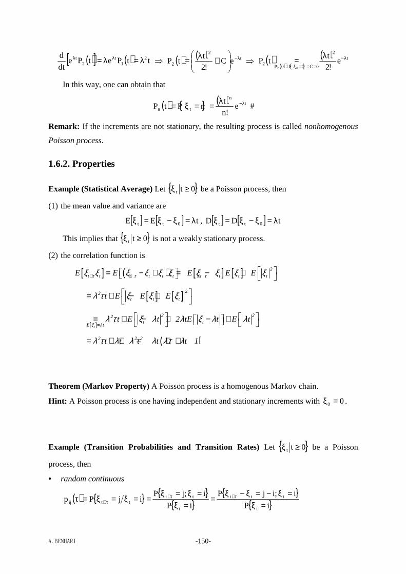
A.BENHARI -150-
( )[ ] ( ) ttPetPedt
d 21
t2
t λ=λ= λλ ⇒ ( ) ( ) t2
2 eC!2
ttP λ−
+λ= ⇒ ( )
( ) ( ) t
2
0C2P0P2 e
!2t
tP02
λ−
===ξ=
λ=
In this way, one can obtain that
( ) ( ) tn
tn e!n
tnPtP λ−λ==ξ= #
Remark: If the increments are not stationary, the resulting process is called nonhomogenous
Poisson process.
1.6.2. Properties
Example (Statistical Average) Let 0tt ≥ξ be a Poisson process, then
(1) the mean value and variance are
[ ] [ ] tEE 0tt λ=ξ−ξ=ξ , [ ] [ ] tDD 0tt λ=ξ−ξ=ξ
This implies that 0tt ≥ξ is not a weakly stationary process.
(2) the correlation function is
[ ] ( ) [ ] [ ] 2
t t t t t t t t t tE E E E Eτ τ τξ ξ ξ ξ ξ ξ ξ ξ ξ ξ+ + + = − + = − +
[ ] [ ] 22t t tt E E Eλ τ ξ ξ ξ = + − +
[ ]t
2 22t t
E tt E t 2 tE t E t
ξ λλ τ ξ λ λ ξ λ λ
= = + − + − +
( )2 2 2t t t t t 1λ τ λ λ λ λτ λ= + + = + +
Theorem (Markov Property) A Poisson process is a homogenous Markov chain.
Hint: A Poisson process is one having independent and stationary increments with 00 =ξ .
Example (Transition Probabilities and Transition Rates) Let 0tt ≥ξ be a Poisson
process, then
• random continuous
( )
iP
i;ijP
iP
i;jPijPp
t
ttt
t
ttttij =ξ
=ξ−=ξ−ξ=
=ξ=ξ=ξ
==ξ=ξ=τ τ+τ+τ+
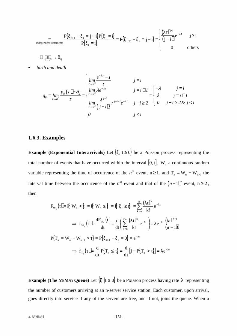
A.BENHARI -151-
( )( )
≥
−λτ
=−=ξ−ξ==ξ
=ξ−=ξ−ξ=
λτ−−
τ+τ+
others0
ije!ijijP
iP
iPijPij
ttt
ttt
incrementstindependen
ij0δ → +→τ
• birth and death
( )
( )
0
ij ij 0ij j i0
j i 1
0
e 1lim j i
j ilim e j i 1pq lim j i 1
0 j i 2 & j ilim e j i 2j i !
0 j i
λτ
τλτ
τ
τλτ
τ
τλλτ δ
λτ λ τ
+
+
+
+
−
→
−
→
−→− − −
→
− = − == +− = = = = + − ≥ <− ≥ −
<
1.6.3. Examples
Example (Exponential Interarrivals) Let 0tt ≥ξ be a Poisson process representing the
total number of events that have occurred within the interval [ ]t,0 , nW a continuous random
variable representing the time of occurrence of the thn event, 1n ≥ , and 1nnn WWT −−= the
interval time between the occurrence of the thn event and that of the ( )1th
n− event, 2n ≥ ,
then
( ) ( )∑+∞
=
λ−λ=≥ξ=≤=<=nk
tk
tnnW e!k
tnPtWPtWPtF
n
⇒ ( ) ( ) ( ) ( )( )!1n
tee
!k
t
dt
d
dt
tdFtf
1nt
nk
tk
W
Wn
n −λλ=
λ==−
λ−∞+
=
λ−∑
λτ−τ+− ==ξ−ξ=τ>−= e0PWWTP tt1nnn
⇒ ( ) [ ] λτ−λ=τ>−τ
=τ≤τ
=τ eTP1d
dTP
d
df nnTn
Example (The M/M/n Queue) Let 0tt ≥ξ be a Poisson process having rate λ representing
the number of customers arriving at an n-server service station. Each customer, upon arrival,
goes directly into service if any of the servers are free, and if not, joins the queue. When a
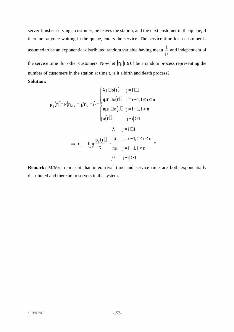
A.BENHARI -152-
server finishes serving a customer, he leaves the station, and the next customer in the queue, if
there are anyone waiting in the queue, enters the service. The service time for a customer is
assumed to be an exponential-distributed random variable having mean µ1
and independent of
the service time for other customers. Now let 0tt ≥η be a random process representing the
number of customers in the station at time t, is it a birth and death process?
Solution:
( )
( )( )( )
( )
>−τ
>−=τ+µτ
≤≤−=τ+µτ
+=τ+λτ
==η=η=τ τ+
1ijo
ni,1ijon
ni1,1ijoi
1ijo
ijPp ttij
⇒ ( )
>−
>−=µ
≤≤−=µ
+=λ
=τ
τ=
+→τ
1ij0
ni,1ijn
ni1,1iji
1ij
plimq ij
0ij #
Remark: M/M/n represent that interarrival time and service time are both exponentially
distributed and there are n servers in the system.
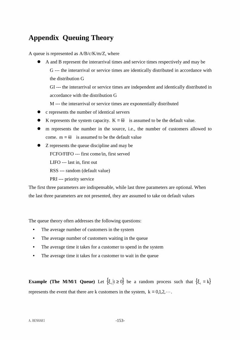
A.BENHARI -153-
Appendix Queuing Theory
A queue is represented as A/B/c/K/m/Z, where
A and B represent the interarrival times and service times respectively and may be
G --- the interarrival or service times are identically distributed in accordance with
the distribution G
GI --- the interarrival or service times are independent and identically distributed in
accordance with the distribution G
M --- the interarrival or service times are exponentially distributed
c represents the number of identical servers
K represents the system capacity. +∞=K is assumed to be the default value.
m represents the number in the source, i.e., the number of customers allowed to
come. +∞=m is assumed to be the default value
Z represents the queue discipline and may be
FCFO/FIFO --- first come/in, first served
LIFO --- last in, first out
RSS --- random (default value)
PRI --- priority service
The first three parameters are indispensable, while last three parameters are optional. When
the last three parameters are not presented, they are assumed to take on default values
The queue theory often addresses the following questions:
• The average number of customers in the system
• The average number of customers waiting in the queue
• The average time it takes for a customer to spend in the system
• The average time it takes for a customer to wait in the queue
Example (The M/M/1 Queue) Let 0tt ≥ξ be a random process such that kt =ξ
represents the event that there are k customers in the system, L,2,1,0k = .

A.BENHARI -154-
Suppose the average arrival rate of customers to the system and the average service rate are λ
and ( )λ>µ respectively, then the transition rates are given by
( )
( )
( )
>−=ττ
−=µ=τ
τ+µτ
+=λ=τ
τ+λτ
=τ
=ξ=ξ=
+
+
+
+
→τ
→τ
→τ
τ+
→τ
1ij0o
lim
1ijo
lim
1ijo
lim
ijPlimq
0
0
0
tt
0ij
Thus, the process is a birth and death process. It follows from the Fokker-Planck equation that
( ) ( ) ( )( ) ( ) ( ) ( ) ( )
≥µ+µ+λ−λ=′µ+λ−=′
+− 1jtptptptp
tptptp
1jj1jj
100
+∞→⇒
t ( )
≥µ+µ+λ−λ=µ+λ−=
∞+
∞∞−
∞∞
1jppp0
pp0
1jj1j
10
⇒
≥µ−λ=µ−λ=µ−λ
∞+
∞∞∞−
∞∞
1jpppp
pp
1jjj1j
10
⇒ ∞∞
µλ= 0
j
j pp 1p
0jj =∑
⇒∞+
=
∞
j
j 1p
µλ
µλ−=∞
The average number of customers in the system is then given
λ−µλ=
µλ−µ
λ=
µλ
µλ−=
µλ
µλ−== ∑∑∑
∞+
=
∞+
=
∞+
=
∞
1k11kkpL
0k
k
0k
k
0kk
The average number of customers in the queue is then given
( ) ( ) ( )λ−µµλ=
µλ−
µλ=−−=−= ∞
+∞
=
∞∑22
01k
kQ1
1p1Lp1kL
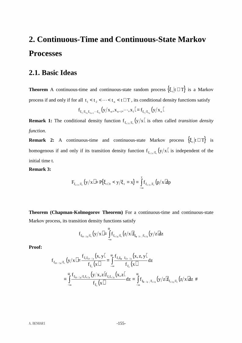
A.BENHARI -155-
2. Continuous-Time and Continuous-State Markov
Processes
2.1. Basic Ideas
Theorem A continuous-time and continuous-state random process Ttt ∈ξ is a Markov
process if and only if for all Ttttt n21 ∈<<<< L , its conditional density functions satisfy
( ) ( )n11nn xyfx,,x,xyfntt1t1ntntt ξξ−ξξξξ =
−LL
Remark 1: The conditional density function ( )xyftt ξξ τ+
is often called transition density
function.
Remark 2: A continuous-time and continuous-state Markov process Ttt ∈ξ is
homogenous if and only if its transition density function ( )xyftt ξξ τ+
is independent of the
initial time t.
Remark 3:
( ) ( )∫∞−
ξξτ+ξξ τ+τ+==ξ<ξ=
y
tt dpxpfxyPxyFtttt
Theorem (Chapman-Kolmogorov Theorem) For a continuous-time and continuous-state
Markov process, its transition density functions satisfy
( ) ( ) ( )∫+∞
∞−ξξξξξξ γ+τ+γ+γ+γ+τ+
= dzzyfxzfxyftttttt
Proof:
( )( )
( )( )
( )∫+∞
∞− ξ
ξξξ
ξ
ξξξξ
γ+τ+γ+γ+τ+
γ+τ+== dz
xf
y,z,xf
xf
y,xfxyf
t
ttt
t
tt
tt
( ) ( )( )∫
+∞
∞− ξ
ξξξξξ γ+γ+γ+τ+= dzxf
z,xfz,xyf
t
ttttt ( ) ( )∫+∞
∞−ξξξξ γ+γ+γ+τ+
= dzxzfzyftttt
#
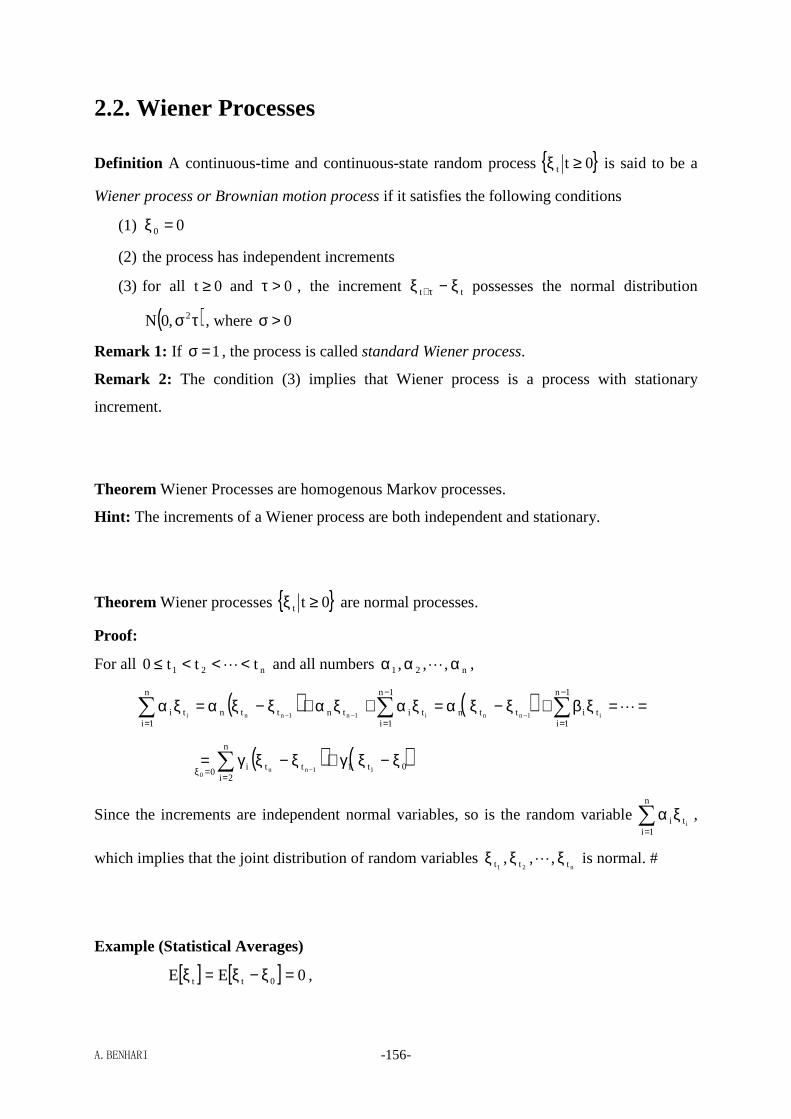
A.BENHARI -156-
2.2. Wiener Processes
Definition A continuous-time and continuous-state random process 0tt ≥ξ is said to be a
Wiener process or Brownian motion process if it satisfies the following conditions
(1) 00 =ξ
(2) the process has independent increments
(3) for all 0t ≥ and 0>τ , the increment tt ξ−ξ τ+ possesses the normal distribution
( )τσ2,0N , where 0>σ
Remark 1: If 1=σ , the process is called standard Wiener process.
Remark 2: The condition (3) implies that Wiener process is a process with stationary
increment.
Theorem Wiener Processes are homogenous Markov processes.
Hint: The increments of a Wiener process are both independent and stationary.
Theorem Wiener processes 0tt ≥ξ are normal processes.
Proof:
For all n21 ttt0 <<<≤ L and all numbers n21 ,,, ααα L ,
( ) ( ) ==ξβ+ξ−ξα=ξα+ξα+ξ−ξα=ξα ∑∑∑−
=
−
==−−−
L1n
1itittn
1n
1ititnttn
n
1iti i1nni1n1nni
( ) ( )0t1
n
2itti
0 11nn0
ξ−ξγ+ξ−ξγ= ∑==ξ −
Since the increments are independent normal variables, so is the random variable ∑=
ξαn
1iti i
,
which implies that the joint distribution of random variables n21 ttt ,,, ξξξ L is normal. #
Example (Statistical Averages)
[ ] [ ] 0EE 0tt =ξ−ξ=ξ ,

A.BENHARI -157-
[ ] [ ] [ ] tEDD 22
t0tt σ=ξ=ξ−ξ=ξ
[ ] ( )[ ] [ ] [ ] tEEEE 22
t
2
tttttt σ=ξ=ξ+ξξ−ξ=ξξ τ+τ+
[ ][ ] [ ] τ+
=ξξ
ξξ=ρτ+
ττ+
t
t
DD
E
tt
t
Remark: Wiener processes 0tt ≥ξ are not weakly stationary.
Example Let 0tt ≥ξ be a Wiener process, what’s its transition density function
( ) ?xyftt
=ξξ τ+
Solution:
( ) =<ξ<ξ+ξ−ξ=<ξ<ξ= τ+τ+ξξ τ+x;yPx;yPx,yF tttttttt
( ) ( )∫ ∫∫∫∞− ∞−
=+=<<+
ξ=ξ−ξ=−==<<+=
τ+
y x
UVvt,vus
xv,yvu
UVV,U
dtdst,tsfdudvv,ufxV;yVUPttt
Recall that ( )τσξ−ξ= τ+2
tt ,0N~U , ( )t,0N~V 2t σξ= , and U and V are independent, we
have
( ) ( ) ( ) ( ) ( )( )
t2
x
2
xy
VUUV
22
2
2
2
tt
tte
t2
1e
2
1xfxyfx,xyf
xy
x,yFx,yf σ
−τσ
−−ξξ
ξξσπσπτ
=−=−=∂∂
∂= τ+
τ+
⇒ ( ) ( )( )
( )
( )τσ
−−
σ−
σ−
τσ−
−
ξ
ξξξξ σπτ
=
σπ
σπσπτ== τ+
τ+
2
2
2
2
2
2
2
2
t
tt
tt
2
xy
t2
x
t2
x
2
xy
e2
1
et2
1
et2
1e
2
1
xf
x,yfxyf
⇒ ( ) ( )τσ=ξξ τ+
2,xNxyftt
#
Remark: The problem can be solved in another way. Recall that
( ) ( )ρσσµµ ,,,,N~Y,X 22
2121 ⇒ ( ) ( ) ( )
ρ−σµ+µ−
σσρ= 22
2211
2XY 1,xNxyf
since
( )( )τ+σξ−ξ=ξ τ+τ+ t,0N~ 20tt , ( )t,0N~ 2
0tt σξ−ξ=ξ
[ ][ ] [ ] ( ) τ+
=στ+σ
σ=ξξ
ξξ=ρτ+
τ+
t
t
tt
t
DD
E22
2
tt
tt
then, the joint distribution of ( )tt ,ξξ τ+ are
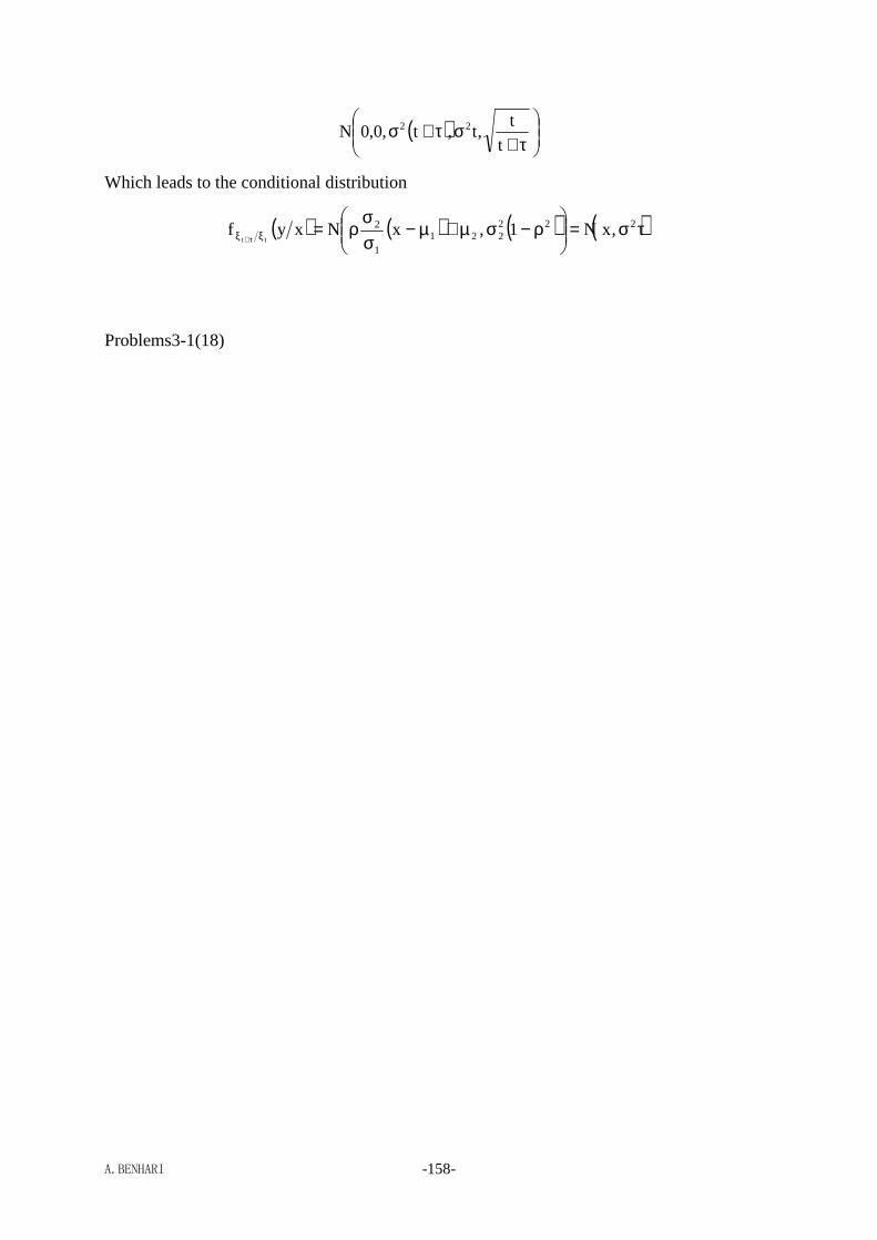
A.BENHARI -158-
( )
τ+στ+σ
t
t,t,t,0,0N 22
Which leads to the conditional distribution
( ) ( ) ( ) ( )τσ=
ρ−σµ+µ−
σσ
ρ=ξξ τ+
222221
1
2 ,xN1,xNxyftt
Problems3-1(18)

A.BENHARI -159-
Hidden Markov Models
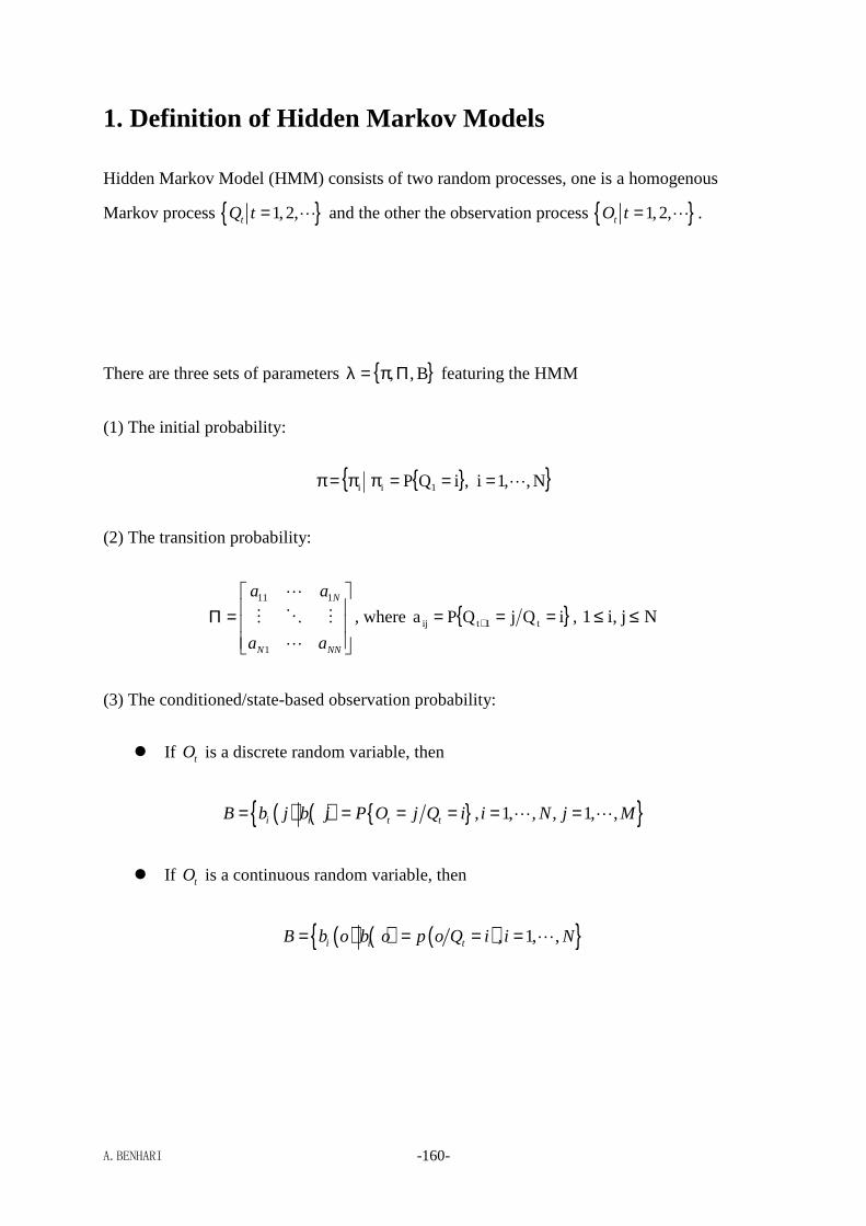
A.BENHARI -160-
1. Definition of Hidden Markov Models
Hidden Markov Model (HMM) consists of two random processes, one is a homogenous
Markov process 1,2,tQ t = L and the other the observation process 1,2,tO t = L .
There are three sets of parameters B,,Ππ=λ featuring the HMM
(1) The initial probability:
N,,1i,iQP 1ii L===ππ=π
(2) The transition probability:
11 1
1
N
N NN
a a
a a
Π =
L
M O M
L
, where iQjQPa t1tij === + , Nj,i1 ≤≤
(3) The conditioned/state-based observation probability:
If tO is a discrete random variable, then
( ) ( ) , 1, , , 1, ,i i t tB b j b j P O j Q i i N j M= = = = = =L L
If tO is a continuous random variable, then
( ) ( ) ( ) , 1, ,i i tB b o b o p o Q i i N= = = = L
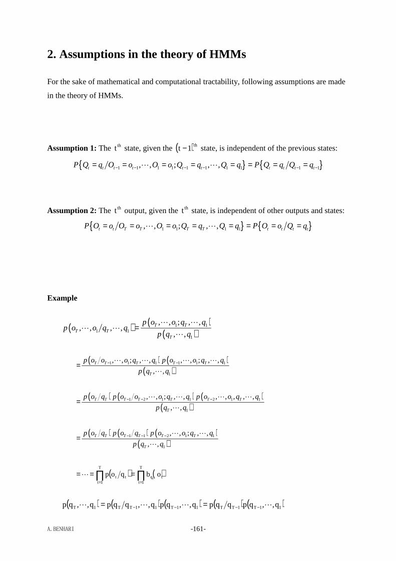
A.BENHARI -161-
2. Assumptions in the theory of HMMs
For the sake of mathematical and computational tractability, following assumptions are made
in the theory of HMMs.
Assumption 1: The tht state, given the ( )th1t − state, is independent of the previous states:
1 1 1 1 1 1 1 1 1 1, , ; , ,t t t t t t t t t tP Q q O o O o Q q Q q P Q q Q q− − − − − −= = = = = = = =L L
Assumption 2: The tht output, given the tht state, is independent of other outputs and states:
1 1 1 1, , ; , ,t t T T T T t t t tP O o O o O o Q q Q q P O o Q q= = = = = = = =L L
Example
( ) ( )( )
1 11 1
1
, , ; , ,, , , ,
, ,T T
T TT
p o o q qp o o q q
p q q=
L LL L
L
( ) ( )( )
1 1 1 1 1 1
1
, , ; , , , , ; , ,
, ,T T T T T
T
p o o o q q p o o q q
p q q− −=L L L L
L
( ) ( ) ( )( )
1 2 1 1 2 1 1
1
, , ; , , , , , , ,
, ,T T T T T T T
T
p o q p o o o q q p o o q q
p q q− − −=
L L L L
L
( ) ( ) ( )( )
1 1 2 1 1
1
, , ; , ,
, ,T T T T T T
T
p o q p o q p o o q q
p q q− − −=
L L
L
( ) ( )∏∏==
===T
1ttq
T
1ttt obqop
tL
( ) ( ) ( ) ( ) ( )11T1TT11T11TT1T q,,qpqqpq,,qpq,,qqpq,,qp LLLL −−−− ==

A.BENHARI -162-
( ) ( ) ∏∏==
− −π===
T
2tqqq
T
2t1tt1 t1t1
aqqpqpL
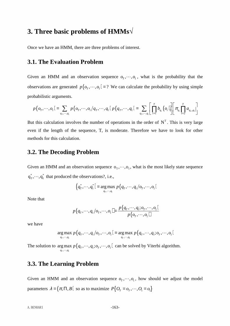
A.BENHARI -163-
3. Three basic problems of HMMs√
Once we have an HMM, there are three problems of interest.
3.1. The Evaluation Problem
Given an HMM and an observation sequence 1, ,To oL , what is the probability that the
observations are generated ( )1, , ?Tp o o =L We can calculate the probability by using simple
probabilistic arguments.
( ) ( ) ( )1
1 1 1 1, ,
, , , , , , , ,T
T T T Tq q
p o o p o o q q p q q= ∑L
L L L L ( )1 1
1, , 1 2t t t
T
T T
q t q q qq q t t
b o a−
= =
=
∑ ∏ ∏L
π
But this calculation involves the number of operations in the order of TN . This is very large
even if the length of the sequence, T, is moderate. Therefore we have to look for other
methods for this calculation.
3.2. The Decoding Problem
Given an HMM and an observation sequence 1T o,,o L , what is the most likely state sequence
*1
*T q,,q L that produced the observations?, i.e.,
( ) ( )1
* *1 1 1
, ,, , arg max , , , ,
T
T T Tq q
q q p q q o o=L
L L L
Note that
( ) ( )( )
1 11 1
1
, , ; , ,, , , ,
, ,T T
T TT
p q q o op q q o o
p o o=
L LL L
L
we have
( ) ( )1 1
1 1 1 1, , , ,
arg max , , , , arg max , , ; , ,T T
T T T Tq q q q
p q q o o p q q o o=L L
L L L L
The solution to ( )1
1 1, ,
arg max , , ; , ,T
T Tq q
p q q o oL
L L can be solved by Viterbi algorithm.
3.3. The Learning Problem
Given an HMM and an observation sequence 1, ,To oL , how should we adjust the model
parameters ( ), ,B= Πλ π so as to maximize 1 1, ,T TP O o O o= =L
A.BENHARI -164-
( )1arg max , ,Tp o oλλ
λ ∗ = L
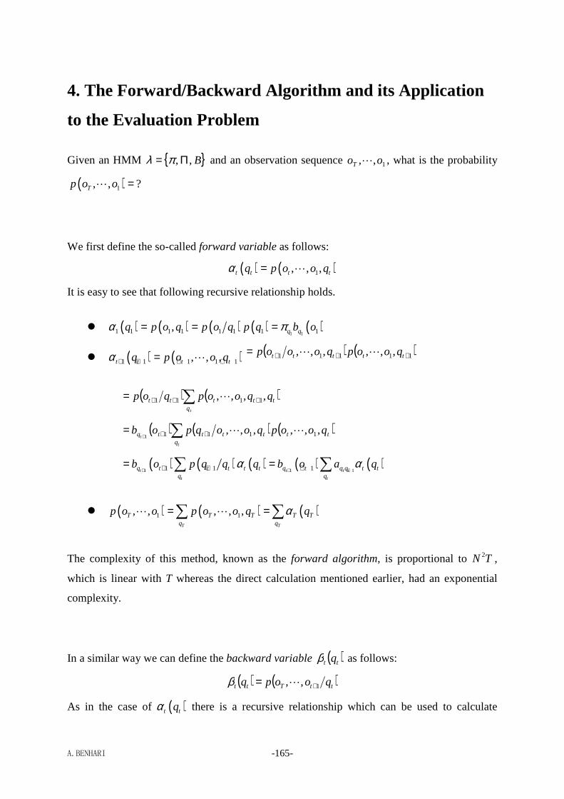
A.BENHARI -165-
4. The Forward/Backward Algorithm and its Applicati on
to the Evaluation Problem
Given an HMM B,,Π= πλ and an observation sequence 1,, ooT L , what is the probability
( )1, , ?Tp o o =L
We first define the so-called forward variable as follows:
( ) ( )1, , ,t t t tq p o o qα = L
It is easy to see that following recursive relationship holds.
( ) ( ) ( ) ( ) ( )1 11 1 1 1 1 1 1 1, q qq p o q p o q p q b oα π= = =
( ) ( )1 1 1 1 1, , ,t t t tq p o o qα + + + += L( ) ( )11111 ,,,,,, +++= ttttt qoopqooop LL
( ) ( )∑ +++=tq
ttttt qqoopqop ,,,, 1111 L
( ) ( ) ( )∑ +++=
t
tq
ttttttq qoopqooqpob ,,,,,, 11111LL
( ) ( ) ( ) ( ) ( )1 1 11 1 1t t t t
t t
q t t t t t q t q q t tq q
b o p q q q b o a qα α+ + ++ + += =∑ ∑
( ) ( ) ( )1 1, , , , ,T T
T T T T Tq q
p o o p o o q qα= =∑ ∑L L
The complexity of this method, known as the forward algorithm, is proportional to TN2 ,
which is linear with T whereas the direct calculation mentioned earlier, had an exponential
complexity.
In a similar way we can define the backward variable ( )tt qβ as follows:
( ) ( )ttTtt qoopq 1,, += Lβ
As in the case of ( )t tqα there is a recursive relationship which can be used to calculate

A.BENHARI -166-
( )tt qβ efficiently.
( ) 1=TT qβ
( ) ( )ttTtt qoopq 1,, += Lβ ( )∑+
++=1
11,,,tq
tttT qqoop L
( ) ( )∑+
+++++=1
11112 ,,,,,tq
tttttttT qqopqqooop L
( ) ( )∑+
++++=1
1112 ,,,tq
tttttT qqopqoop L ( ) ( ) ( )∑+
+++++=1
11111 ,tq
ttttttt qqpqqopqβ
( ) ( )∑+
+++++=1
11111
t
ttq
qqtttt aqopqβ ( ) ( )∑+
++ +++=1
11 111
t
tttq
qqtqtt aobqβ
( ) ( ) ( ) ( )1 1
1 1 1 2 1 1 1 1, , , , , , , , ,T T Tq q
p o o p o o q p o o o q p o q= =∑ ∑L L L
( ) ( ) ( ) ( ) ( )1 1
1 1
2 1 1 1 1 1 1 1, ,T q qq q
p o o q p o q p q q b oβ π= =∑ ∑L
Further we can see that,
( )tttT qoooop ,,,,,, 11 LL + ( ) ( )tttttT qoopqooooP ,,,,,,,, 111 LLL +=
( ) ( ) ( ) ( )1 1, , , , ,T t t t t t t t tp o o q p o o q q qβ α+= =L L
Therefore this gives another way to calculate ( )1,, oop T L , by using both forward and
backward variables as given in the following equation,
( ) ( ) ( ) ( )1 1, , , , ,t t
T T t t t t tq q
p o o p o o q q qα β= =∑ ∑L L
The above equation is very useful, specially in deriving the formulas required for gradient
based training.
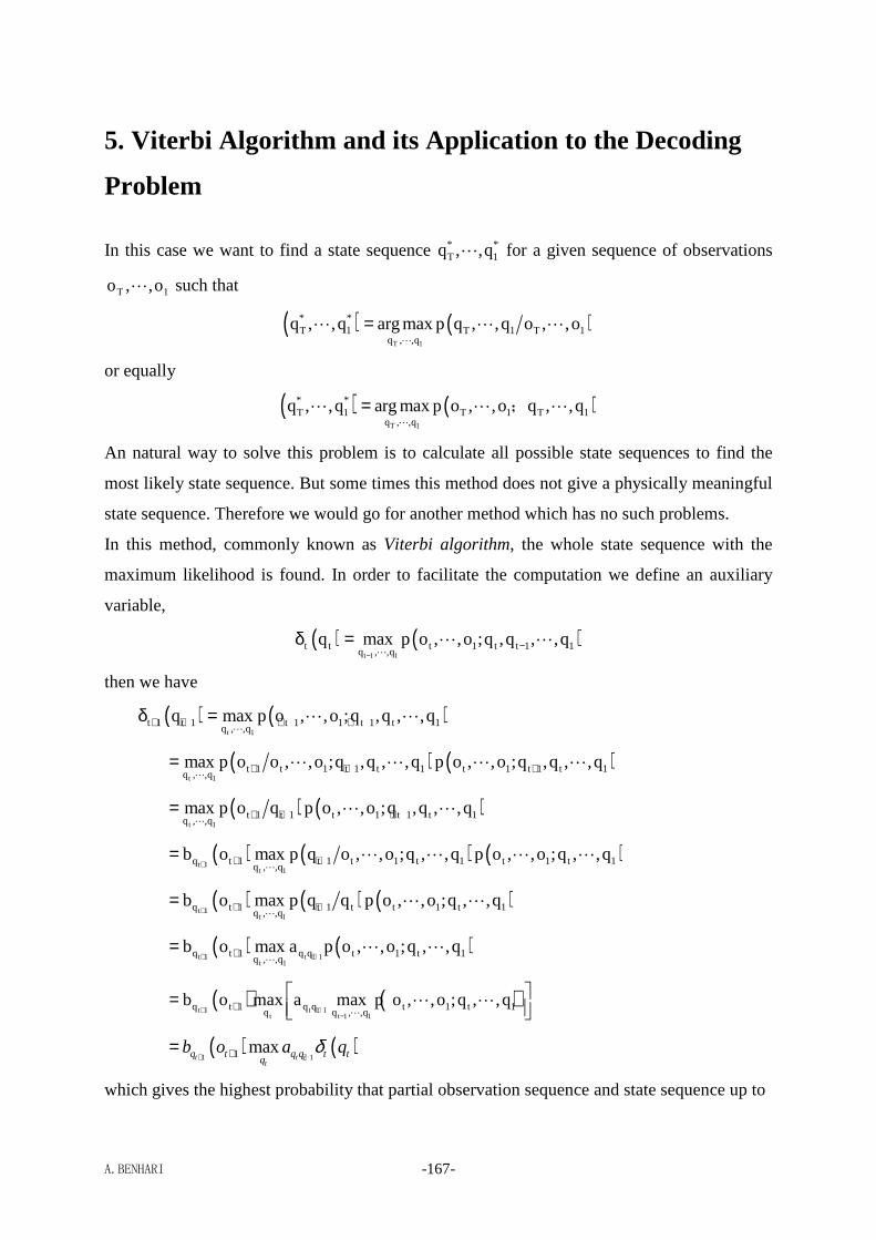
A.BENHARI -167-
5. Viterbi Algorithm and its Application to the Decoding
Problem
In this case we want to find a state sequence *1
*T q,,q L for a given sequence of observations
1T o,,o L such that
( ) ( )T 1
* *T 1 T 1 T 1
q , ,qq , ,q arg max p q , ,q o , ,o=
L
L L L
or equally
( ) ( )T 1
* *T 1 T 1 T 1
q , ,qq , ,q arg max p o , ,o q , ,q=
L
L L L;
An natural way to solve this problem is to calculate all possible state sequences to find the
most likely state sequence. But some times this method does not give a physically meaningful
state sequence. Therefore we would go for another method which has no such problems.
In this method, commonly known as Viterbi algorithm, the whole state sequence with the
maximum likelihood is found. In order to facilitate the computation we define an auxiliary
variable,
( ) ( )t 1 1
t t t 1 t t 1 1q , ,q
q max p o , ,o ;q ,q , ,q−
−δ =L
L L
then we have
( ) ( )t 1
t 1 t 1 t 1 1 t 1 t 1q , ,q
q max p o , ,o ;q ,q , ,q+ + + +δ =L
L L
( ) ( )t 1
t 1 t 1 t 1 t 1 t 1 t 1 t 1q , ,qmax p o o , ,o ;q ,q , ,q p o , ,o ;q ,q , ,q+ + +=L
L L L L
( ) ( )t 1
t 1 t 1 t 1 t 1 t 1q , ,qmax p o q p o , ,o ;q ,q , ,q+ + +=L
L L
( ) ( ) ( )t 1
t 1q t 1 t 1 t 1 t 1 t 1 t 1
q , ,qb o max p q o , ,o ;q , ,q p o , ,o ;q , ,q
+ + +=L
L L L L
( ) ( ) ( )t 1
t 1q t 1 t 1 t t 1 t 1
q , ,qb o max p q q p o , ,o ;q , ,q
+ + +=L
L L
( ) ( )t 1 t t 1
t 1q t 1 q q t 1 t 1
q , ,qb o max a p o , ,o ;q , ,q
+ ++=L
L L
( ) ( )t 1 t t 1
t t 1 1q t 1 q q t 1 t 1
q q , ,qb o max a max p o , ,o ;q , ,q
+ +−
+ = L
L L
( ) ( )1 11 max
t t tt
q t q q t tq
b o a qδ+ ++=
which gives the highest probability that partial observation sequence and state sequence up to
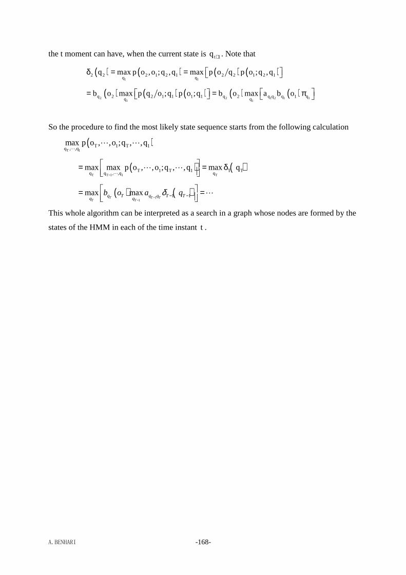
A.BENHARI -168-
the t moment can have, when the current state is 1tq + . Note that
( ) ( ) ( ) ( )1 1
2 2 2 1 2 1 2 2 1 2 1q q
q max p o ,o ;q ,q max p o q p o ;q ,qδ = =
( ) ( ) ( ) ( ) ( )2 2 1 2 1 1
1 1q 2 2 1 1 1 1 q 2 q q q 1 q
q qb o max p q o ;q p o ;q b o max a b o = = π
So the procedure to find the most likely state sequence starts from the following calculation
( )T 1
T 1 T 1q , ,qmax p o , ,o ;q , ,q
LL L
( ) ( )T T 1 1 T
T 1 T 1 T Tq q , ,q q
max max p o , ,o ;q , ,q max q−
= = δ L
L L
( ) ( )1
11 1max max
T T TT T
q T q q T Tq q
b o a qδ−
−− −
= =
L
This whole algorithm can be interpreted as a search in a graph whose nodes are formed by the
states of the HMM in each of the time instant t .
A.BENHARI -169-
6. Baum-Welch Algorithm and its Application to the
Learning Problem
Generally, the learning problem is how to adjust the HMM parameters so that the given set of
observations (called the training set) is represented by the model in the best way for the
intended application. Thus it would be clear that the “quantity” we wish to optimize during
the learning process can be different from application to application. In other words there may
be several optimization criteria for learning, out of which a suitable one is selected depending
on the application.
There are two main optimization criteria for the learning problem: Maximum Likelihood
(ML) and Maximum Mutual Information (MMI). The solutions to the learning problem under
each of those criteria is described below.
6.1. Maximum Likelihood (ML) Criterion
In ML we try to maximize the probability of a given sequence of observations 1,, ooT L , given
a HMM ( ),A,Bλ Π= . This probability is the total likelihood of the observations and can be
expressed mathematically as
( ) ( )1, ,TL p o oλλ = L
Then the ML criterion can be given as,
( )λλλ
Lmaxarg=∗
However there is no known way to analytically solve for the model ( ),A,Bλ Π= , which
maximize the quantity ( )λL . But we can choose model parameters such that it is locally
maximized, using an iterative procedure, like Baum-Welch method or a gradient based
method, which are described below.
6.2. Baum-Welch Algorithm
To describe the Baum-Welch algorithm, (also known as Forward-Backward algorithm), we
need to define two more auxiliary variables, in addition to the forward and backward variables
defined in a previous section. These variables can however be expressed in terms of the
forward and backward variables.
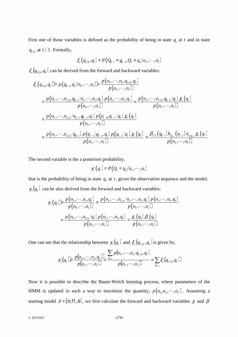
A.BENHARI -170-
First one of those variables is defined as the probability of being in state tq at t and in state
1+tq at 1+t . Formally,
( ) ( )1 1 1 1, , , ,t t t t t t t Tq q P Q q Q q o o+ + += = = Lξ
( )ttt qq ,1+ξ can be derived from the forward and backward variables:
( ) ( ) ( )( )
1 11 1 1
1
, , , ,, , , ,
, ,T t t
t t t t t TT
p o o q qq q p q q o o
p o oξ +
+ += =L
LL
( ) ( )( )
( ) ( )( )
1 1 1 1 1 1
1 1
, , , , , , , , , , , ,
, , , ,T t t t t t t T t t t t t
T T
p o o q o o q p o o q p o o q q q
p o o p o o
χ+ + + += =L L L L
L L
( ) ( ) ( )( )
2 1 1 1 1
1
, , , , ,
, ,T t t t t t t t t t
T
p o o o q q p o q q q
p o o
χ+ + + + +=L
L
( ) ( ) ( ) ( )( )
2 1 1 1 1
1
, , ,
, ,T t t t t t t t t t
T
p o o q p o q q p q q q
p o o
χ+ + + + +=L
L
( ) ( ) ( )( )
1 11 1 1
1, ,t t tt t q t q q t t
T
q b o a q
p o o
β χ+ ++ + +=
L
The second variable is the a posteriori probability,
( ) ( )1, ,t t t t Tq P Q q o o= = Lγ
that is the probability of being in state tq at t , given the observation sequence and the model.
( )tt qγ can be also derived from the forward and backward variables:
( ) ( )( )
1
1
, , ,
, ,T t
t tT
p o o qq
p o oγ =
L
L
( ) ( )( )
1 1 1
1
, , , , , , , ,
, ,T t t t t t
T
p o o o o q p o o q
p o o+=
L L L
L
( ) ( )( )
( ) ( )( )
1 1
1 1
, , , , ,
, , , ,T t t t t t t t t
T T
p o o q p o o q q q
p o o p o o
χ β+= =L L
L L
One can see that the relationship between ( )tt qγ and ( )ttt qq ,1+ξ is given by,
( ) ( )( )
( )
( ) ( )∑∑
+
++
+
===1
1 ,,,
,,,,
,,
,,,1
1
11
1
1
t
t
qttt
T
qttT
T
tTtt qq
oop
qqoop
oop
qoopq ξγ
L
L
L
L
Now it is possible to describe the Baum-Welch learning process, where parameters of the
HMM is updated in such a way to maximize the quantity, ( )1 2, , , Tp o o oL . Assuming a
starting model ( )B,,Π= πλ , we first calculate the forward and backward variables χ and β

A.BENHARI -171-
using the recursions, and then ξ and γ . Next step is to update the HMM parameters
according to the following equations, known as re-estimation formulas.
( )1q qπ γ=),
( )
( )∑
∑−
=
−
=+
=+ 1
1
1
11,
1 T
ttt
T
tttt
q
qqa
tt
γ
ξ)
, ( )( )
( )1 ,
1
ˆ t
t
t tt T o o
q T
t tt
q
b oq
γ
γ
≤ ≤ =
=
=∑
∑
( ) ( )( ) ( )
11
11
Rr
rq R
r
q r
q
q
γπ
γ=
=
=∑
∑∑
),
( ) ( )( ) ( )
1
1 11
1 1
,R T
rt
r tqq R T
rt
r t
q qa
q
ξ
γ
−
= =′ −
= =
′=∑∑
∑∑
)
( ) ( ) ( ) ( )( )1, ,r r rt t Tq P Q q o oγ = = L , ( ) ( ) ( ) ( )( )1 1, , , ,r r r
t t t Tq q P Q q Q q o oξ +′ ′= = = L
( )
( ) ( )( ) ( )
11
1
1 1
Rr
k rq R T
rt
r t
q
q
γπ
γ=
−
= =
=∑
∑∑
)
A.BENHARI -172-
Second-Order Processes and Random Analysis

A.BENHARI -173-
1. Second-Order Random Variables and Hilbert Spaces
Theorem Let H be the collection of all second-order random variables defined on a
probability space ( )P,,ΠΩ , then
(1) H is a linear space
(2) for all H, ∈ηξ , let [ ]ηξ=ηξ E, , then ( )••,,H is a Hilbert space.
Hint:
[ ] ( )( )[ ] [ ] [ ] [ ]ξη+η+ξ≤η+ξη+ξ=η+ξ ECC2ECECCCCCECCE 21
22
2
22
12121
2
21
[ ] [ ] [ ] [ ] +∞<ηξ+η+ξ≤−
22
21
22
2
22
1InequalitySwartchCauchy
EECC2ECEC
⇒ H is a linear space
10P ==ξ ⇔ [ ] 0E2 =ξ ; [ ] [ ] ξη=ηξ=ηξ=ηξ ,EE,
⇒ H is an inner space
In measure theory, one can prove that a Cauchy sequence in H is convergent
⇒ H is a complete inner space, i.e., Hilbert space
Remark 1: [ ]2E, ξ=ξξ=ξ is then a norm.
Remark 2: Since
0nnlim ξ=ξ
+∞→ def= [ ] 0Elim,limlim
2
0nn
0n0nn
0nn
=ξ−ξ=ξ−ξξ−ξ=ξ−ξ+∞→+∞→+∞→
the convergence in H is often called mean square convergence.
A.BENHARI -174-
2. Second-Order Random Processes
Definition A random process Ttt ∈ξ is called a second-order random process if for all
Tt ∈ , tξ is a second-order random variable, i.e., [ ] +∞<ξ 2E .
Theorem Let Ttt ∈ξ be a second-order random process and ( )21 tt21 ,t,t ξξ=Γ , then for
all all Tt,,t,t n21 ∈L , the matrix
( ) ( ) ( )( ) ( ) ( )
( ) ( ) ( )
ΓΓΓ
ΓΓΓΓΓΓ
=Γ
nn2n1n
n22212
n12111
t,tt,tt,t
t,tt,tt,t
t,tt,tt,t
L
MOMM
L
L
is nonnegative
definite.
Proof:
For all numbers n21 ,,, ααα L ,
( )
( ) ( ) ( )( ) ( ) ( )
( ) ( ) ( )
=
α
αα
ΓΓΓ
ΓΓΓΓΓΓ
ααα
n
2
1
nn2n1n
n22212
n12111
n21
t,tt,tt,t
t,tt,tt,t
t,tt,tt,t
M
L
MOMM
L
L
L
( ) ( )( )[ ]=ξαξα=ξαξα=Γαα= ∑∑∑∑∑∑= == == =
n
1i
n
1jjjii
n
1i
n
1jjjii
n
1i
n
1jjiji E,t,t
( )( ) 0EE
2n
1jii
n
1i
n
1jjjii ≥
ξα=
ξαξα= ∑∑∑
== = #
2.1. Orthogonal Increment Random Processes
Definition A second-order random process Ttt ∈ξ is called an orthogonal increment
random process if for all Ttttt 4321 ∈<≤< , 0,3412 tttt =ξ−ξξ−ξ .
Example Let Ttt ∈ξ be an orthogonal increment random process with [ )+∞= ,aT and
A.BENHARI -175-
0a =ξ , then
(1) For all 21 tta ≤≤ , we have
0,,121121 ttatttt =ξ−ξξ−ξ=ξ−ξξ
(2) For all Ttt 21 ∈≤ , we have
2
tttttttttttttt 11111121112121,,,,, ξ=ξξ=ξξ+ξ−ξξ=ξ+ξ−ξξ=ξξ
(3) For all Ttt 21 ∈≤ , we have
2
t
2
ttttttttttttt
2
tt 1211122122121212,,,,, ξ−ξ=ξξ+ξξ−ξξ−ξξ=ξ−ξξ−ξ=ξ−ξ
A.BENHARI -176-
3. Random Analysis
3.1. Limits
Definition Let ( ) b,att ∈ξ be a second-order random process and η a second-order random
variable, η=ξ→ t
tt 0
lim is then defined as η−ξ→ t
tt 0
lim , where ( )b,at 0 ∈ .
Theorem η=ξ→ t
tt 0
lim ⇔ the limit stts,tt
,lim00
ξξ→→
exists.
3.2. Continuity
Definition A second-order random process Ttt ∈ξ is said to be continuous at the point
Tt0 ∈ if given any 0>ε , there will be 0>δε such that for all Tt ∈ with εδ<− 0tt ,
ε<ξ−ξ0tt .
Remark 1: If ( ) Tb,at 0 =∈ , tξ is said to be continuous at 0t if 0lim0
0tt
tt=ξ−ξ
→.
Remark 2: 0lim0
0tt
tt=ξ−ξ
→ is often denoted by
00
tttt
lim ξ=ξ→
.
Theorem If 0
0tt
ttlim ξ=ξ→
, then [ ] [ ]0
0tt
ttEElim ξ=ξ
→.
Proof:
[ ] [ ] [ ] 0EEEEE000000 tttt
2
tttttttt →ξ−ξ=ξ−ξ≤ξ−ξ≤ξ−ξ=ξ−ξ →
Theorem If 0
0tt
ttlim ξ=ξ→
, 0
0ss
sslim ξ=ξ→
, then 00
00stst
ss,tt,,lim ξξ=ξξ
→→.
Proof:
00 stst ,, ξξ−ξξ
000000 sststtsstt ,,, ξ−ξξ+ξξ−ξ+ξ−ξξ−ξ=
000000 sststtsstt ,,, ξ−ξξ+ξξ−ξ+ξ−ξξ−ξ≤
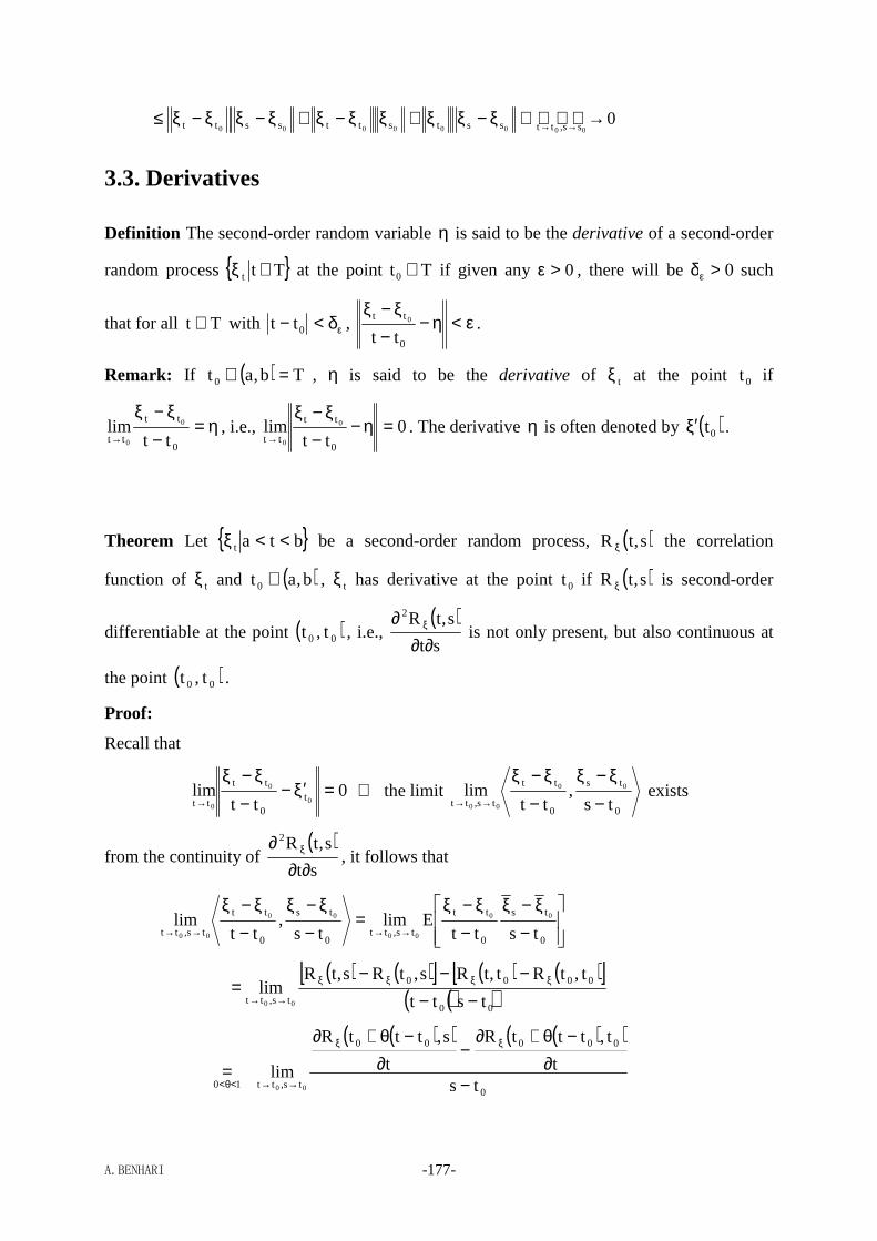
A.BENHARI -177-
000000000 ss,ttsststtsstt →ξ−ξξ+ξξ−ξ+ξ−ξξ−ξ≤ →→
3.3. Derivatives
Definition The second-order random variable η is said to be the derivative of a second-order
random process Ttt ∈ξ at the point Tt0 ∈ if given any 0>ε , there will be 0>δε such
that for all Tt ∈ with εδ<− 0tt , ε<η−−
ξ−ξ
0
tt
tt0 .
Remark: If ( ) Tb,at 0 =∈ , η is said to be the derivative of tξ at the point 0t if
η=−
ξ−ξ→
0
tt
tt ttlim 0
0
, i.e., 0tt
lim0
tt
tt
0
0
=η−−
ξ−ξ→
. The derivative η is often denoted by ( )0tξ′ .
Theorem Let btat <<ξ be a second-order random process, ( )s,tR ξ the correlation
function of tξ and ( )b,at 0 ∈ , tξ has derivative at the point 0t if ( )s,tR ξ is second-order
differentiable at the point ( )00 t,t , i.e., ( )st
s,tR2
∂∂∂ ξ is not only present, but also continuous at
the point ( )00 t,t .
Proof:
Recall that
0tt
lim0
0
0t
0
tt
tt=ξ′−
−ξ−ξ
→ ⇔ the limit
0
ts
0
tt
ts,tt ts,
ttlim 00
00 −ξ−ξ
−ξ−ξ
→→ exists
from the continuity of ( )st
s,tR2
∂∂∂ ξ , it follows that
−ξ−ξ
−ξ−ξ
=−
ξ−ξ−
ξ−ξ→→→→
0
ts
0
tt
ts,tt0
ts
0
tt
ts,tt tsttElim
ts,
ttlim 00
00
00
00
( ) ( )[ ] ( ) ( )[ ]( )( )00
0000
ts,tt tstt
t,tRt,tRs,tRs,tRlim
00 −−−−−
= ξξξξ
→→
( )( ) ( )( )
0
00000
ts,tt10 tst
t,tttR
t
s,tttR
lim00 −
∂−θ+∂
−∂
−θ+∂
=
ξξ
→→<θ<
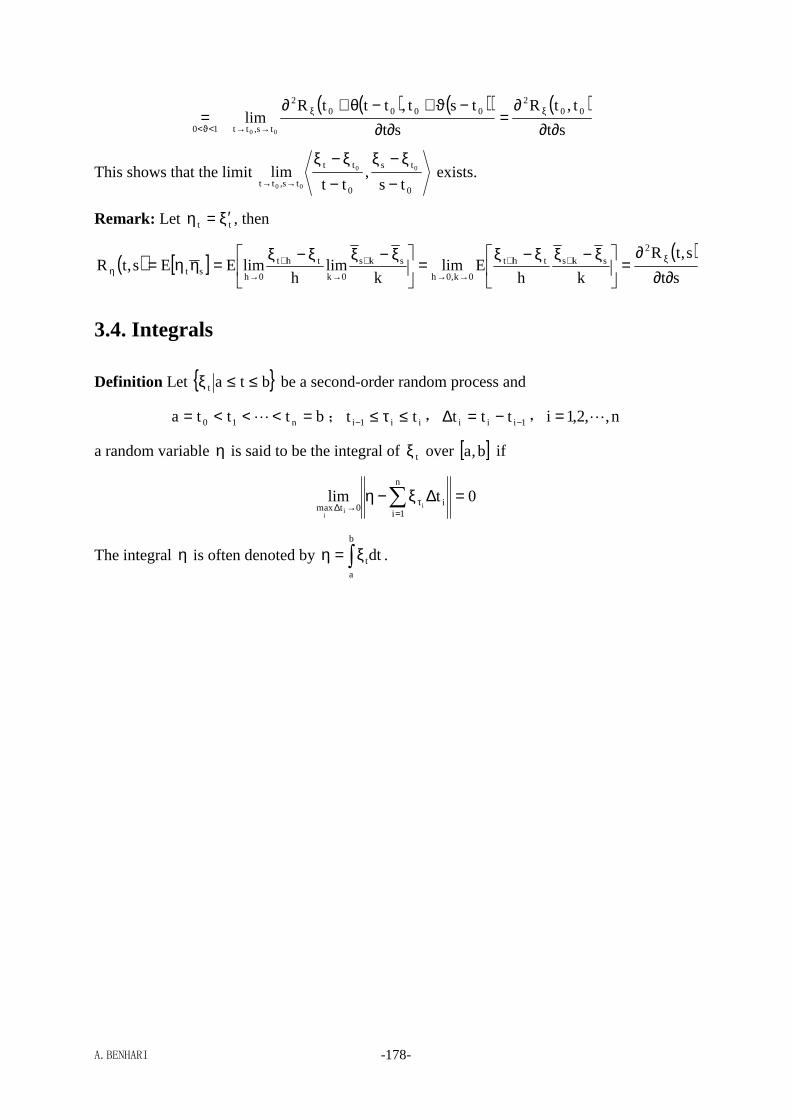
A.BENHARI -178-
( ) ( )( ) ( )st
t,tR
st
tst,tttRlim 00
20000
2
ts,tt10 00 ∂∂∂
=∂∂
−ϑ+−θ+∂= ξξ
→→<ϑ<
This shows that the limit 0
ts
0
tt
ts,tt ts,
ttlim 00
00 −ξ−ξ
−ξ−ξ
→→ exists.
Remark: Let tt ξ′=η , then
( ) [ ] ( )st
s,tR
khElim
klim
hlimEEs,tR
2
skstht
0k,0h
sks
0k
tht
0hst ∂∂
∂=
ξ−ξξ−ξ=
ξ−ξξ−ξ=ηη= ξ++
→→
+
→
+
→η
3.4. Integrals
Definition Let btat ≤≤ξ be a second-order random process and
bttta n10 =<<<= L ; ii1i tt ≤τ≤− , 1iii ttt −−=∆ , n,,2,1i L=
a random variable η is said to be the integral of tξ over [ ]b,a if
0tlimn
1ii
0tmax ii
i
=∆ξ−η ∑=
τ→∆
The integral η is often denoted by ∫ξ=ηb
a
tdt .

A.BENHARI -179-
Stationary Processes
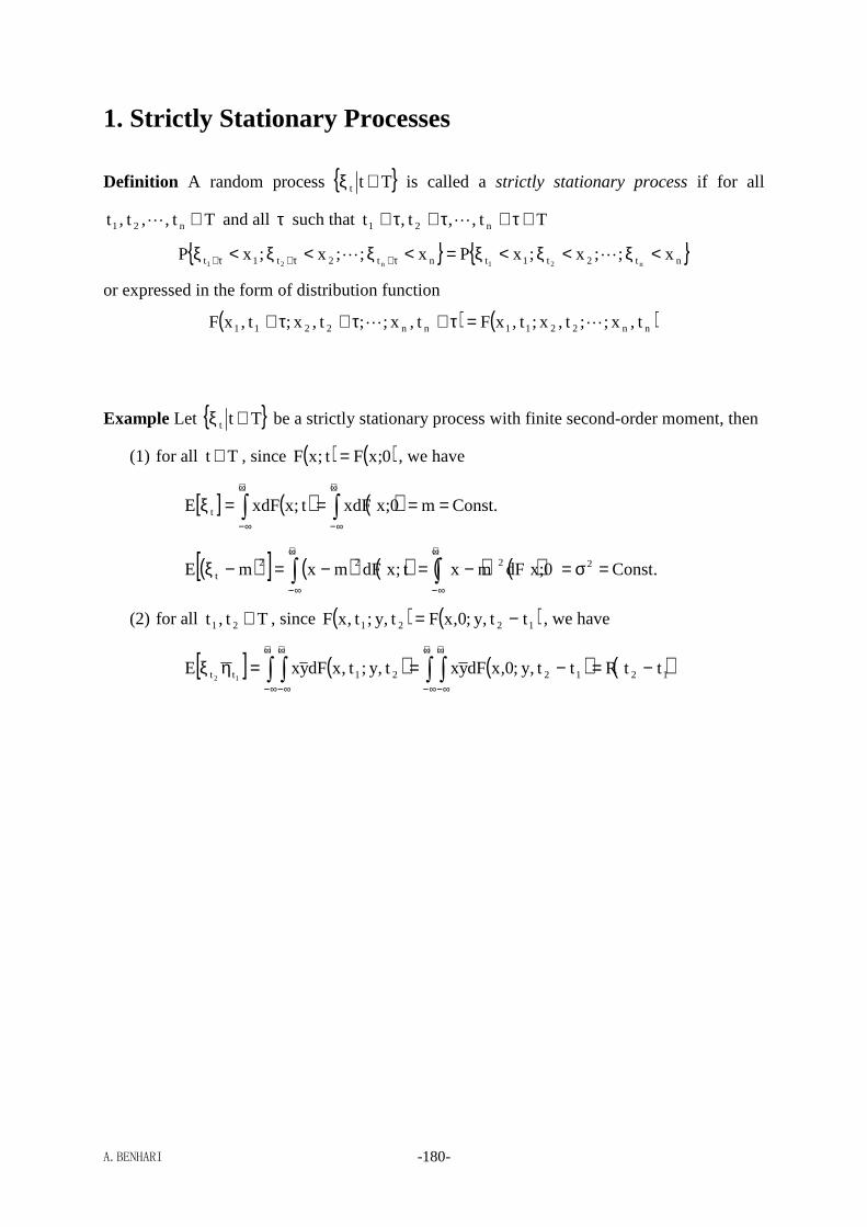
A.BENHARI -180-
1. Strictly Stationary Processes
Definition A random process Ttt ∈ξ is called a strictly stationary process if for all
Tt,,t,t n21 ∈L and all τ such that Tt,,t,t n21 ∈τ+τ+τ+ L
nt2t1tnt2t1t x;;x;xPx;;x;xPn21n21
<ξ<ξ<ξ=<ξ<ξ<ξ τ+τ+τ+ LL
or expressed in the form of distribution function
( ) ( )nn2211nn2211 t,x;;t,x;t,xFt,x;;t,x;t,xF LL =τ+τ+τ+
Example Let Ttt ∈ξ be a strictly stationary process with finite second-order moment, then
(1) for all Tt ∈ , since ( ) ( )0;xFt;xF = , we have
[ ] ( ) ( ) .Constm0;xxdFt;xxdFE t ====ξ ∫∫+∞
∞−
+∞
∞−
( )[ ] ( ) ( ) ( ) ( ) .Const0;xdFmxt;xdFmxmE 2222t =σ=−=−=−ξ ∫∫
+∞
∞−
+∞
∞−
(2) for all Tt,t 21 ∈ , since ( ) ( )1221 tt,y;0,xFt,y;t,xF −= , we have
[ ] ( ) ( ) ( )121221tt ttRtt,y;0,xdFyxt,y;t,xdFyxE12
−=−==ηξ ∫ ∫∫ ∫+∞
∞−
+∞
∞−
+∞
∞−
+∞
∞−
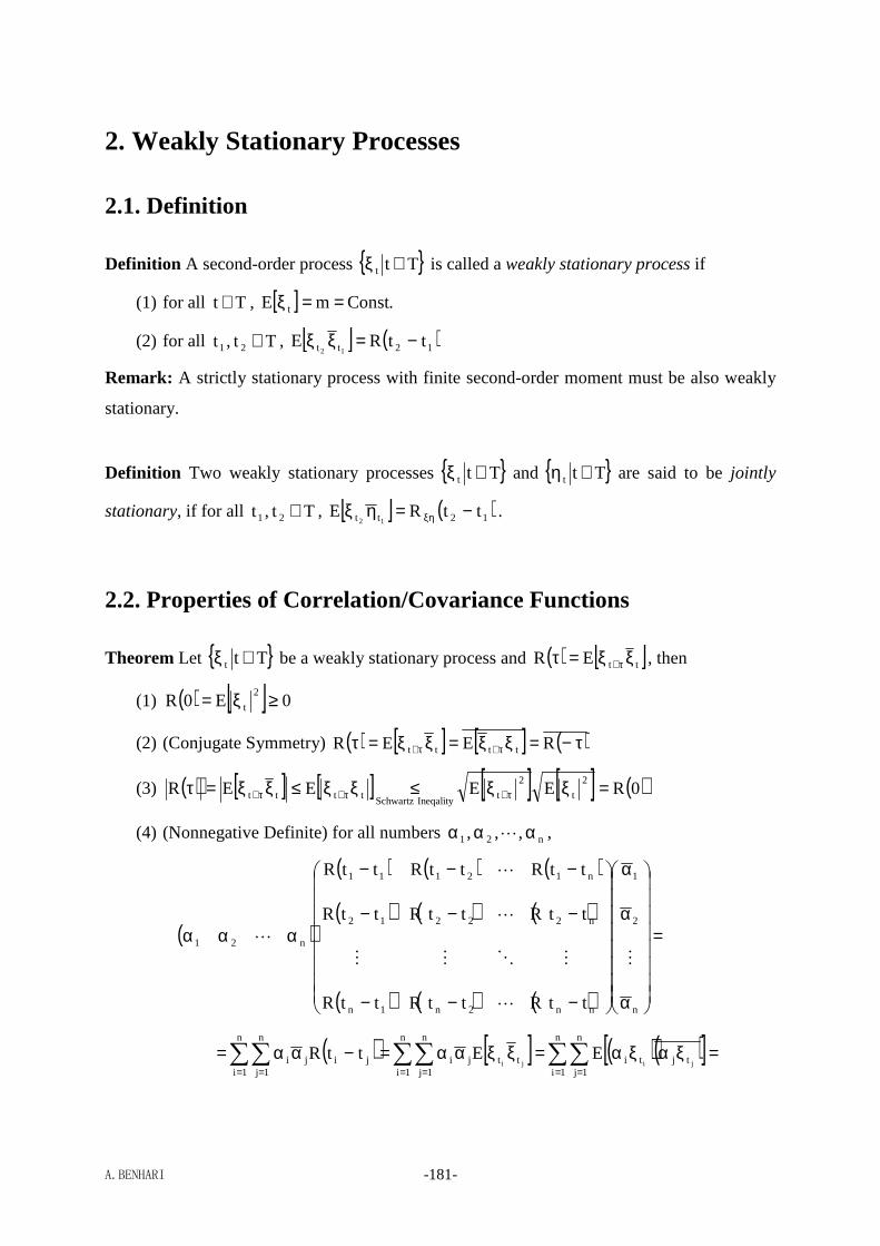
A.BENHARI -181-
2. Weakly Stationary Processes
2.1. Definition
Definition A second-order process Ttt ∈ξ is called a weakly stationary process if
(1) for all Tt ∈ , [ ] .ConstmE t ==ξ
(2) for all Tt,t 21 ∈ , [ ] ( )12tt ttRE12
−=ξξ
Remark: A strictly stationary process with finite second-order moment must be also weakly
stationary.
Definition Two weakly stationary processes Ttt ∈ξ and Ttt ∈η are said to be jointly
stationary, if for all Tt,t 21 ∈ , [ ] ( )12tt ttRE12
−=ηξ ξη .
2.2. Properties of Correlation/Covariance Functions
Theorem Let Ttt ∈ξ be a weakly stationary process and ( ) [ ]ttER ξξ=τ τ+ , then
(1) ( ) [ ] 0E0R2
t ≥ξ=
(2) (Conjugate Symmetry) ( ) [ ] [ ] ( )τ−=ξξ=ξξ=τ τ+τ+ REER tttt
(3) ( ) [ ] [ ] [ ] [ ] ( )0REEEER2
t
2
tIneqalitySchwartz
tttt =ξξ≤ξξ≤ξξ=τ τ+τ+τ+
(4) (Nonnegative Definite) for all numbers n21 ,,, ααα L ,
( )
( ) ( ) ( )
( ) ( ) ( )
( ) ( ) ( )
=
α
α
α
−−−
−−−
−−−
ααα
n
2
1
nn2n1n
n22212
n12111
n21
ttRttRttR
ttRttRttR
ttRttRttR
M
L
MOMM
L
L
L
( ) [ ] ( )( )[ ]=ξαξα=ξξαα=−αα= ∑∑∑∑∑∑= == == =
n
1i
n
1jtjti
n
1i
n
1jttji
n
1i
n
1jjiji jiji
EEttR
A.BENHARI -182-
( )( ) 0EE2n
1iti
n
1i
n
1jtjti iji
≥
ξα=
ξαξα= ∑∑∑
== =
Remark: Cauchy-Schwarz inequality: [ ] [ ] [ ]22EEE ηξ≤ξη
Theorem Let Ttt ∈ξ and Ttt ∈η be two jointly stationary processes and
( ) [ ]ttER ηξ=τ τ+ξη , then.
(1) ( ) [ ] [ ] ( )τ−=ηξ=ηξ=τ ηξτ+τ+ξη REER tttt
(2) ( ) [ ] [ ] [ ] [ ] ( ) ( )0R0REEEER2
t
2
tIneqalitySchwartz
tttt ηξτ+τ+τ+ξη =ηξ≤ηξ≤ηξ=τ
2.3. Periodicity
Theorem (Periodicity) Let +∞<<∞−ξ tt be a weakly stationary process, tξ is periodic
with period T if and only if its correlation function ( )τξR is periodic with period T.
Hint:
[ ] [ ] [ ] [ ]tTt2t
2Tt
2
tTt E2EEE ξξ−ξ+ξ=ξ−ξ +++ ( ) ( )[ ]TR0R2 ξξ −=
2.4. Random Analysis
For a weakly stationary process, the questions of random analysis such as whether the process
is continuous, differentiable or integrable are all dependent on its correlation function.
Theorem Let btat <<ξ be a weakly stationary process and ( )τξR its correlation function,
tξ has derivatives within the open interval ( )b,a if ( )τ′′ξR is present and continuous at the
point 0=τ .
Remark: Let tt ξ′=η , then
[ ] [ ] [ ]0
h
EElim
hElim
hlimEE tht
0h
tht
0h
tht
0ht =ξ−ξ=
ξ−ξ=
ξ−ξ=η +
→
+
→
+
→

A.BENHARI -183-
( ) [ ] ( ) ( ) ( )stRst
stR
st
s,tREs,tR
22
st −′′−=∂∂
−∂=
∂∂∂
=ηη= ξξξ
η ⇒ ( ) ( )τ′′−=τ ξη RR
This shows that tη is also weakly stationary.
2.5. Ergodicity (Statistical Average = Time Average)
Definition Let +∞<<∞−ξ tt be a weakly stationary random process and
[ ]tE ξ=µ ξ , ( ) [ ]ttER ξξ=τ τ+ξ (statistical average)
∫−
+∞→ξ=ξ
T
T
tT
t dtT2
1lim , ∫
−τ++∞→τ+ ξξ=ξξ
T
T
ttT
tt dtT2
1lim (time average)
(1) the mean of tξ is said to be ergodic if 1P t =µ=ξ ξ
(2) the correlation function of tξ is said to be ergodic if ( ) 1RP tt =τ=ξξ ξτ+
(3) tξ is said to be ergodic if both of its mean and correlation function are ergodic
Remark: Ergodicity means that statistical average is equal to time average.
Theorem The mean of a weakly stationary random process +∞<<∞−ξ tt is ergodic if
and only if
( )[ ] ( ) 0dCT2
1T
1limdR
T21
T
1lim
T2
0T
T2
0
2
T=ττ
τ−=τµ−τ
τ− ∫∫ ξ+∞→ξξ+∞→
where ( ) ( ) 2RC ξξξ µ−τ=τ .
Proof:
Note that
[ ] [ ] ξ−
+∞→−
+∞→µ=ξ=
ξ=ξ ∫∫
T
T
tT
T
T
tT
t dtET2
1limdt
T2
1limEE
we have
1P t =µ=ξ ξ ⇔
[ ] [ ] [ ] 2T
T
s
T
T
t2T
22
tt
2
t dsdtT4
1limEEDE0 ξ
−−+∞→ξξ µ−
ξξ=µ−ξ=ξ=µ−ξ= ∫∫
A.BENHARI -184-
[ ] ( ) 2T
T
T
T2T
2T
T
T
T
st2TdtdsstR
T4
1limdtdsE
T4
1lim ξ
− −ξ+∞→ξ
− −+∞→
µ−
−=µ−
ξξ= ∫ ∫∫ ∫
( ) 2
T2qpT2,T2qpT22Tqst,pst
dpdqqR2
1
T4
1lim ξ
<−<−<+<−ξ+∞→=−=+
µ−
= ∫∫
( ) ( ) 2T2
0
qT2
qT2
0
T2
qT2
qT22T
dqqRdpdqqRdpT8
1lim ξξ
−
+−−ξ
+
−−+∞→
µ−
+
= ∫ ∫∫ ∫
( ) ( ) ( ) 2T2
0T
2T2
02T
dqqRT2
q1
T
1limdqqRqT2
T2
1lim ξξ+∞→ξξ+∞→
µ−
−=µ−−= ∫∫
( )[ ] ( )∫∫ ξ+∞→ξξ+∞→
−=µ−
−=T2
0T
T2
0
2
TdqqC
T2
q1
T
1limdqqR
T2
q1
T
1lim #
Theorem The correlation function of a weakly stationary random process +∞<<∞−ξ tt
is ergodic if and only if
( ) ( )[ ] 0dqRqBT2
q1
T
1lim
T2
0
2
T=τ−
−∫ ξϕ+∞→
where ( ) [ ] [ ]ttqtqttqt EEqB ξξξξ=ϕϕ= τ++τ+++ϕ .
Proof:
Let ttt ξξ=ϕ τ+ , then
[ ] [ ] ( )τ=ξξ=ϕ ξτ+ REE ttt
[ ] [ ] ( )∫ ∫ ∫ ∫+∞
∞−
+∞
∞−
+∞
∞−
+∞
∞−τ+τ+ τ+τ+=ξξξξ=ϕϕ dxdydzdws,s,t,t;w,z,y,xxyzwfEE ssttst
( )∫ ∫ ∫ ∫+∞
∞−
+∞
∞−
+∞
∞−
+∞
∞−
τ−τ+−= dxdydzdw0,,st,st;w,z,y,xxyzwf
This shows that tϕ is at least weakly stationary. It follows from the preceding theorem that
[ ] ( ) 1RPEP tttt =τ=ξξ=ϕ=ϕ ξτ+ ⇔ ( ) ( )[ ] 0dqRqBT2
q1
T
1lim
T2
0
2
T=τ−
−∫ ξϕ+∞→ #
2.6. Spectrum Analysis & White Noise
Definition Let +∞<<∞−ξ tt be a random process, the spectrum of tξ is defined as
A.BENHARI -185-
( )( )[ ]T2
T,FElimS
2
T
ω=ω ξ
+∞→ξ
where ( ) ∫−
ω−ξ ξ=ω
T
T
tjt dteT,F is the Fourier transform of tξ . Note that ( )T,F ωξ is also a
random process.
Theorem (Wiener-Khintchine Theorem) Let +∞<<∞−ξ tt be a weakly stationary
random process, ( )τξR the correlation function and ( )ωξS the spectrum of tξ , then
( ) ( )∫+∞
∞−
ωτ−ξξ ττ=ω deRS j , ( ) ( )∫
+∞
∞−
ωτξξ ωω
π=τ deS
2
1R j
Example ( )ωξS is a real-valued function.
Proof:
( ) ( ) ( ) ( ) ( )ω=ττ=ττ−=ττ=ω ξ
+∞
∞−
ωτ−ξ
+∞
∞−
ωτξ
+∞
∞−
ωτξξ ∫∫∫ SdeRdeRdeRS jjj #
Definition (White Noise) A weakly stationary process +∞<<∞−ξ tt is said to be a white
noise process if its spectrum is flat, i.e., ( ) ( ).ConstS 2σ=ωξ
Remark: Since
( ) 1de j =ττδ∫+∞
∞−
ωτ− ⇔ ( )τδ=τπ ∫
+∞
∞−
ωτde2
1 j
we have
( ) ( ) ( )τδσ=τσπ
=τωπ
=τ ∫∫+∞
∞−
ωτ+∞
∞−
ωτξξ
2j2j de2
1deS
2
1R
A.BENHARI -186-
3. Discrete Time Sequence Analysis: Auto-Regressive and
Moving-Average (ARMA) Models
3.1. Definition
Definition Let ( )nx be a zero-mean white noise, i.e., ( )[ ] 0nxE = , ( ) ( )[ ] ( )mnxmnxE 2xδσ=+ ,
then
(1) a random sequence ( )ny is said to be in accordance with an auto-regressive (AR) model
of order K if it can be expressed as
( ) ( ) ( )nxknyny 0
K
1kk β=−α+∑
=
(2) a random sequence ( )ny is said to be in accordance with a moving-average (MA) model
of order M if it can be expressed as
( ) ( )∑=
−β=M
0mm mnxny
(3) a random sequence ( )ny is said to be in accordance with an auto-regressive and
moving-average (ARMA) model of order ( )M,K if it can be expressed as
( ) ( ) ( )∑∑==
−β=−α+M
0mm
K
1kk mnxknyny
Remark: The power spectrum of white noise:
( ) ( ) ( ) 2x
m
mj2x
m
mjx
j ememReS σ=δσ== ∑∑+∞
−∞=
ω−+∞
−∞=
ω−ω
3.2. Transition Functions
Definition (Transition Functions) Given an ARMA model
( ) ( ) ( )∑∑==
−β=−α+M
0mm
K
1kk mnxknyny
let ( )∑
∑
=
−
=
−
α+
β=
K
1k
kk
M
0m
mm
z1
zzH and maxz the largest pole of ( )zH , if 1zmax < , then the model is said
to be causal and stable and ( )zH is called the transition function of the model.

A.BENHARI -187-
Remark 1: From now on, the ARMA models we encounter in this lecture are all assumed to
be causal and stable, unless declared something else.
Remark 2: If ( )zH is the transition function of an ARMA model, then ( ) ( )[ ]zHZnh 1−= is
called the impulse response of the model. It can be easily proven that
( ) 0nh = for 0n < (causal) and ( ) +∞<∑+∞
=0n
2nh (stable)
Remark 3: For AR models,
( )∑
=
−α+
β=
K
1k
kk
0
z1zH ⇒ ( )nh is of infinite duration (Infinite Impulse Response, IIR)
For MR model,
( ) ∑=
−β=M
0m
mmzzH ⇒ ( )nh is of finite duration (Finite Impulse Response, FIR)
Remark 4: ( )nh can also be solved from the difference equation
( ) ( ) ( )( )
<=
−δβ=−α+ ∑∑==
0nallfor0nh
mnknhnhM
0mm
K
1kk
Example What are the impulse responses for the following models?
(1) ( )1AR
( ) ( ) ( )nx1nyny β=−α− , 1<α
⇒ ( )1z1
zH −α−β= , α>z ⇒ ( ) ( )nu
z1Znh n
11 βα=
α−β= −
−
(2) ( )2AR
( ) ( ) ( ) ( )nx2ny1nyny 21 =−α−−α−
⇒ ( ) ( ) ( ) ( )n2nh1nhnh 21 δ=−α−−α− , ( ) 0nh = for all 0n <
⇒ ( ) 10h = , ( ) 11h α= , ( ) ( ) ( )2nh1nhnh 21 −α+−α= , 2n ≥
Definition ( )ny is said to be the stationary solution/output of an AMAR model if it is given
by ( ) ( ) ( )∑+∞
=
−=0k
knxkhny , where ( )nh is the impulse response of the model.
A.BENHARI -188-
3.3. Mathematical Expectations
Theorem Assume that ( )ny is the stationary solution of an ARMA model and ( )nh the
impulse response of the model. It follows from ( ) ( ) ( )∑+∞
=
−=0k
knxkhny that
• mean value:
( )[ ] ( ) ( ) ( ) ( )[ ] 0knxEkhknxkhEnyE0k0k
y =−=
−==µ ∑∑+∞
=
+∞
=
• correlation function:
( ) ( ) ( )[ ] ( ) ( ) ( ) ( )
−
−+=+= ∑∑
∞+
=
∞+
= 0q0py qnxqhpmnxphEnymnyEmR
( ) ( ) ( ) ( )[ ] ( ) ( ) ( )∑∑∑∑+∞
=
+∞
=
+∞
=
+∞
=
+−δσ=−+−=0q 0p
2x
0q 0p
mpqqhphpmnxqnxEqhph
( ) ( ) ( )mRmqhqh h2x
0q
2x σ=+σ= ∑
+∞
=
where ( ) ( ) ( )∑+∞
=+=
0qh mqhqhmR .
• variance:
( ) ( ) ( )∑+∞
=σ=σ==σ
0n
22xh
2xy
2y nh0R0R
• correlation coefficient or standard correlation function:
( ) ( ) ( )( )0R
mRmRm
h
h2y
yy =
σ=ρ
• spectrum:
( ) ( ) ( ) ( )∑ ∑∑+∞
−∞=
ω−+∞
=
+∞
−∞=
ω−ω
+σ==m
mj
0k
2x
m
jy
jy emkhkhemReS
( ) ( ) ( ) ( ) ( )∑∑∑∑+∞
=
ω−+∞
=
ω
+=
+∞
−∞=
+ω−+∞
=
ω σ=+σ=0n
nj
0k
kj2x
mknm
kmj
0k
kj2x enhekhemkhekh
( )
2
K
1k
jkk
M
0m
jmm
2x
2j2x
e1
eeH
∑
∑
=
ω−
=
ω−
ω
α+
βσ=σ=
Remark: It is clear that ( )ny is also a zero-mean weakly stationary random process.
A.BENHARI -189-
Example For ( )1AR ,
( ) ( ) ( )nx1nyny β=−α− , 1<α ⇒ ( ) ( )nunh nβα=
⇒ ( ) ( )( ) 0
1
11
0R
mRm
m
m
2
2
2
m2
h
hy →α=
α−β
α−αβ
==ρ ±∞→
Remark: ( )myρ is said to tail off if ( ) 0mmy →ρ +∞→ .
3.4. Parameter Estimation
Theorem For an ARMA model ( ) ( ) ( )∑∑==
−β=−α+M
0mm
K
1kk mnxknyny , if mn > , then
( ) ( )[ ] ( ) ( ) ( ) ( ) ( ) ( )[ ] ( ) ( ) 0kmnkhkmxnxEkhkmxkhnxEmynxE0k
2x
0k0k
=+−δσ=−=
−= ∑∑∑+∞
=
+∞
=
+∞
=
Remark: The theorem is straightforward because of the causality of the model. The causality
states that the output from the model is only dependent upon the input to the model at present
and in the past and has nothing to do with the input in the future.
3.4.1. Estimation of AR parameters
Example (Auto-Regressive Weights) Given an ( )KAR model:
( ) ( ) ( )nxknyny 0
K
1kk β=−α−∑
=
then for K,,2,1i L= , we have
( ) ( ) ( ) ( ) ( ) ( )inynxinyknyinyny 0
K
1kk −β=−−α−− ∑
=
⇒ ( ) ( )[ ] ( ) ( )[ ] ( ) ( )[ ] 0inynxEinyknyEinynyE 0
K
1kk =−β=−−α−− ∑
=
⇒ ( ) ( )∑=
−α=K
1kyky kiRiR
( ) ( )( )0R
iRi
y
yy =ρ
⇒ ( ) ( )iki y
K
1kyk ρ=−ρα∑
=
The above equations can be expressed in matrix form:

A.BENHARI -190-
( ) ( ) ( )( ) ( ) ( )
( ) ( ) ( )
( ) ( )( ) ( )
( ) ( )
( )( )
( )
ρ
ρρ
=
α
αα
−ρ−ρ
−ρρ−ρρ
=
α
αα
ρ−ρ−ρ
−ρρρ−ρ−ρρ
K
2
1
12K1K
2K11
1K11
02K1K
K201
K110
y
y
y
K
2
1
yy
yy
yy
K
2
1
yyy
yyy
yyy
MM
L
MOMM
L
L
M
L
MOMM
L
L
The parameters K21 ,,, ααα L can be then derived from the solution to the above equations.
Remark: In practice, ( ) ( ) ( )[ ] ( ) ( )∑+−=
−≈−=n
iKnky ikyky
K
1inynyEiR , where K,,2,1i L= .
Example (Variance of White Noise) Given an ( )KAR model:
( ) ( ) ( )nxknynyK
1kk =−α−∑
=
we have
( )[ ] ( ) ( ) ( ) ( ) ( )∑∑∑∑= ===
−αα+α−=
−α−==σ
K
1p
K
1qyqp
K
1kyky
2K
1kk
22x qpRkR20RknynyEnxE
( ) ( ) ( )( ) ( )
( ) ( ) ( )∑∑∑ ∑∑===∑ −α= ==
α+α−=
−αα+α−=
=
K
1pyp
K
1kyky
pRqpR
K
1p
K
1qyqp
K
1kyky pRkR20RqpRkR20R
y
K
1qq
( ) ( )∑=
α−=K
1kyky kR0R
The variance 2xσ can be obtained after the parameters K21 ,,, ααα L have been estimated.
3.4.2. Estimation of MA parameters
Example (Moving Average Weights) Given a ( )MMA model:
( ) ( )∑=
−β=M
0mm mnxny
for M,,1,0i L= , we have
( ) ( ) ( ) ( ) ( ) ( )∑∑∑∑= ===
−−−ββ=
−−β
−β=−M
0m
M
0kkm
M
0kk
M
0mm kinxmnxkinxmnxinyny
⇒ ( ) ( ) ∑∑∑ ∑−
=+
ββ
=ββσ=σ
−
=+
= =ββσ=ββσ=
−+δββσ=iM
0kikk
2x~
,~
iM
0kikk
2x
M
0k
M
0mmk
2xy
~~~mikiR
0
kk0xx
A.BENHARI -191-
Thus, the unknowns M12X
~,,
~,~ ββσ L can be derived from the solutions to the above M+1
equations.
3.4.3. Estimation of ARMA parameters
Example Given an ( )M,KARMA model:
( ) ( ) ( )∑∑==
−β=−α−M
0mm
K
1kk mnxknyny
for K,,2,1i L= , we have
( ) ( ) ( ) ( ) ( ) ( )∑∑==
−−−β=−−−α−−−M
0mm
K
1kk iMnymnxiMnyknyiMnyny
⇒ ( ) ( )[ ] ( ) ( )[ ] ( ) ( )[ ] 0iMnymnxEiMnyknyEiMnynyEM
0mm
K
1kk =−−−β=−−−α−−− ∑∑
==
⇒ ( ) ( )∑=
−+α=+K
1kyky kiMRiMR
( ) ( )( )0R
iRi
y
yy =ρ
⇒ ( ) ( )iMkiM y
K
1kyk +ρ=−+ρα∑
=
The above equations can be expressed in matrix form:
( ) ( ) ( )( ) ( ) ( )
( ) ( ) ( )
( )( )
( )
+ρ
+ρ+ρ
=
α
αα
ρ−+ρ−+ρ
−+ρρ+ρ−+ρ−ρρ
KM
2M
1M
M2KM1KM
K2MM1M
K1M1MM
y
y
y
K
2
1
yyy
yyy
yyy
MM
L
MOMM
L
L
The parameters K21 ,,, ααα L can be then derived from the solutions to the above equations.
Example Given an ( )M,KARMA model:
( ) ( ) ( )∑∑==
−β=−α−M
0mm
K
1kk mnxknyny
if let
( ) ( ) ( )∑=
−α−=K
1kk knynyng
the ( )M,KARMA model can reduces to an ( )MMA model
( ) ( )∑=
−β=M
0mm mnxng
A.BENHARI -192-
the unknowns ( )
ββ
=β
ββ
=βσβ=σ0
MM
0
11x0x
~,,
~,~ L can be then derived from the solutions to
the following equations:
( ) ∑−
=+ββσ=
iM
0kikk
2Xg
~~~iR , M,,1,0i L=
A.BENHARI -193-
4. Problems
(1) An IID process must be strictly stationary.
In fact, let Ttt ∈ξ be an IID process, then
=<ξ<ξ<ξ=<ξ<ξ<ξ τ+τ+τ+τ+τ+τ+ nt2t1tceindependen
nt2t1t xPxPxPx,,x,xPn21n21
LL
nt2t1tceindependen
nt2t1tondistributiidentical
x,,x,xPxPxPxPn21n21
<ξ<ξ<ξ=<ξ<ξ<ξ= LL #
(2) If L,2,1nn =ξ is a discrete random process with [ ] 0E n =ξ , [ ] 22nE σ=ξ and
[ ] 0E mn =ξξ (when mn ≠ ), then
[ ] ( )mnmn0
mnE 2
2
mn −δσ=
≠=σ
=ξξ
This implies that the process L,2,1nn =ξ is a weakly stationary process. #
(3) Let θ be a random variable possessing a uniform distribution over the interval ( )π2,0 and
( ) +∞<<−∞θ+ω=ξξ t,tcosatt , then
for all +∞<<∞− t , we have
[ ] ( ) ( ) 0dyycos2
adxxtcosa
2
1E
2t
txty
2
0
t =π
=+ωπ
=ξ ∫∫π+ω
ω+ω=
π
for all +∞<≤<∞− 21 tt , we have
[ ] ( ) ( ) ( )12
22
0
21
2
tt ttcos2
adxxtcosxtcos
2
aE
12−=+ω+ω
π=ξξ ∫
π
This implies that the process ( ) +∞<<−∞θ+ω=ξξ t,tcosatt is weakly stationary. #
Remark: ( ) ( )
2
coscoscoscos
β−α+β+α=βα
A.BENHARI -194-
(4) Let ( )ts be a periodic function with period T, η be a random variable possessing the
uniform distribution on the interval ( )T,0 and ( ) +∞<<−∞η+ξ t,tst , then
for all +∞<<∞− t , we have
[ ] ( ) ( ) ( ) ( ) ( ) .constdyysT
1dyys
T
1dxxts
T
1dxxfxtsE
T
0yperiodicit
Tt
txty
T
0
t ===+=+=ξ ∫∫∫∫+
+=
+∞
∞−
for all +∞<≤<∞− 21 tt , we have
[ ] ( ) ( ) ( ) ( ) ( ) =++=++=ξξ ∫∫+∞
∞−
T
0
2121tt dxxtsxtsT
1dxxfxtsxtsE
12
( ) ( ) ( ) ( ) ( )12
T
0
12yperiodicit
Tt
t
12xty
ttRdyyttsysT
1dyyttsys
T
1 1
11
−=+−=+−= ∫∫+
+=
This implies that the process ( ) +∞<<−∞η+ξ t,tst is weakly stationary. #
(5) Let +∞<<∞−ξ tt be a random process such that for all +∞<<∞− t ,
−=
=
==ξ
others0
Ik2
1
Ik2
1
kP t
Furthermore, for all 0>τ , if we denote by kA the event that the process changes its values k
times within the period [ )τ+t,t , then
( ) λτ−λτ= e!k
APk
k ,where 0>λ , L,2,1,0k =
Thus,
for all +∞<<∞− t , we have
[ ] ( ) 02
1I
2
1IE t =×−+×=ξ
for all +∞<<<∞− 21 tt , we have
[ ] ( )LL ++++×=ξξ n2202
tt APAPAPIE12
( )LL ++++×− +1n2312 APAPAPI
( ) λτ−+∞
=
λτ− =λτ−××= ∑ 22
0k
k2 eI
!keI , where 12 tt −=τ
A.BENHARI -195-
Note that the above result can also be applied to the case of 12 tt =
This implies that the process is weakly stationary. #
(6) If +∞<<∞−ξ tt is a periodic random process with period T, then its covariance
function ( ) [ ]ttER ξξ=τ τ+ is also a periodic function with period T.
Proof:
• Since the process is periodic with period T, i.e., 1P tTt =ξ=ξ + , we have
[ ] 0E2
tTt =ξ−ξ + .
• From Cauchy-Schwarz inequality and the result obtained in (1), we have
( )[ ] [ ] [ ] 0EEE02
t
2
tTtttTt =ξξ−ξ≤ξξ−ξ≤ τ++τ+τ++τ+ ⇒ ( )[ ] 0E ttTt =ξξ−ξ τ++τ+
• Form the result obtained in (2), we have
( ) ( ) ( )[ ] ( )[ ] 0EERTR ttTtttTt =ξξ−ξ≤ξξ−ξ=τ−+τ τ++τ+τ++τ+ ⇒ ( ) ( )τ=+τ RTR #

A.BENHARI -196-
MartingalesMartingalesMartingalesMartingales
A.BENHARI -197-
1. Simple properties
DefinitionsDefinitionsDefinitionsDefinitions. Let (Ω,K,P) be a probability space. A filtrationfiltrationfiltrationfiltration is any increasing
sequence of sub-σ-algebras of K. We shall denote it by (F n)n≥1 . Usually one adds
to the filtration its tail tail tail tail σσσσ----field, that is the σ-algebra F ∞ defined by F∞ =σ(
U∞
=1n
Fn). Let X:= (Xn)n be a sequence of random variables. We call X adaptedadaptedadaptedadapted if Xn
is Fn-measurable for any positive integer n. The system (Ω,K,P, (F n)n) is called
a stochastic basisa stochastic basisa stochastic basisa stochastic basis.
Example.Example.Example.Example. If we define Fn := σ(X1,X2,…,Xn) , then X is clearly adapted. This
filtration is called the natural filtration natural filtration natural filtration natural filtration given by X.
Definitions.Definitions.Definitions.Definitions. Let X be an adapted sequence. Suppose that Xn ∈ L
1
for any n. Then X
is called
• A supermartingalesupermartingalesupermartingalesupermartingale if E(Xn+1 Fn) ≤ Xn ∀ n;
• A martingalemartingalemartingalemartingale if E(Xn+1 Fn) = Xn ∀ n;
• A submartingalesubmartingalesubmartingalesubmartingale if E(Xn+1 Fn) ≥ Xn ∀ n;
• A semimartingalesemimartingalesemimartingalesemimartingale if X is either supermartingale or martingale or
submartingale.
Remark.Remark.Remark.Remark. If one does not define the filtration, it is understood that he has in
mind the natural filtration. Also notice that a martingale is both a sub- and a
super- martingale and conversely, if X is both sub- and super- martingale, it is a
martingale.
Remark.Remark.Remark.Remark. In the literature the concept of semimartingale is slightly different.
However, we shall use it only in this sense.
Examples.Examples.Examples.Examples.
1. Let ξn be a sequence of i.i.d. r.v. from L
1
and let a = Eξ1. Let Fn =
σ(ξ1,ξ2,…,ξn) and Xn = ξ1 + ξ2 +…+ξn . Then a ≤ 0 ⇒ X is a supermartingale, a =
0 ⇒ X is a martingale and a ≥ 0 ⇒ X is a submartingale. If we think at ξn as
being the gain of a player at the n’th game, then Xn is the gain of the player
ofter n games. So we can understand a supermartingale or a martingale as the
gain in an unfair game and the martingale as the gain in a fair game.
Supermartingale = the game is unfavorable to the player and submartingale =
game favorable to the player.
Proof. E(Xn+1Fn) = E(Xn+ξn+1Fn) = E(XnFn) + E(ξn+1Fn) = Xn + E(ξn+1Fn) (as Xn is Fn -
measurable) = Xn + Eξn+1 (as Xn is independent on Fn ) ⇒ E(Xn+1Fn) = Xn + a . 2. Let ξn be a sequence of non-negative i.i.d. r.v. from L
1
and let a = Eξ1. Let Fn
= σ(ξ1,ξ2,…,ξn) and Xn = ξ1ξ2 … ξn . Then a ≤ 1 ⇒ X is a supermartingale, a =
1 ⇒ X is a martingale and a ≥ 1 ⇒ X is a submartingale.
Proof. Similar. E(Xn+1Fn) = E(Xnξn+1Fn) = XnE(ξn+1Fn) (as Xn is Fn -measurable) =
XnEξn+1 (as Xn is independent on Fn ) ⇒ E(Xn+1Fn) = aXn . 3. Let (Fn)n be a filtration and f ∈ L
1
. Let Xn = E(fFn). Then Xn is a martingale.
The random variable X∞ = E(fF∞) is called the tail of X . Martingales of this
form are called martingales with tail.
A.BENHARI -198-
Proof. E(Xn+1Fn) = E(E(fFn+1)Fn) = E(fFn) (as Fn ⊂ Fn+1) = Xn. 4. A concrete example. Let Ω = (0,1], K = B ((0,1]), P = the Lebesgue measure and
Xn =
]1
,0(1
n
n . Check that this is a non-negative martingale converging to 0 a.s.
but not in L
1
.
5. Another concrete example. Let ξn be i.i.d with the distribution (ε-1+ε1)/2. Let
Fn = σ(ξ1,…,ξn). Let Bn ∈ Fn be such that P(Bn) → 0 as n → ∞ but P(limsup Bn)
= 1. Define the sequence Xn by recurrence as follows: X1=ξ1 and Xn+1 =
Xn(1+ξn+1)+ξn+1
nB1 for n ≥ 1. Then Xn converges in probability to 0 but P(limsupXn =
liminfXn) = 0. That is, Xn diverges almost surely.
Proof. Remark that ξn+1(ω) = -1 and ω∉Bn ⇒ Xn+1(ω)=0 hence Xn+1(ω) ≠ 0 ⇒ ξn+1(ω) = 1,Xn(ω) ≠ 0 or ω ∈ Bn. That is, Xn+1 ≠ 0 ⊂ ξn+1 = 1,Xn ≠ 0 ∪ Bn ⇒ P(Xn+1 ≠ 0) ≤ P( ξn+1 = 1,Xn≠0 ∪ Bn) ≤ P(ξn+1= 1, Xn ≠ 0) + P(Bn) = P(Xn ≠ 0)P(ξn+1=1) + P(Bn) =
P(Xn ≠ 0)/2 + P(Bn).
Let pn = P(Xn≠0) and qn = P(Bn). So pn+1 ≤ pn/2 + qn ∀ n and qn → 0. Aplying the
recurrence many times we see that pn+1 ≤ 2-1
pn + qn ≤ 2-2
pn-1+ 2
-1
qn-1 + qn ≤ 2-3
pn-2 + 2
-2
qn-
2 + 2
-1
qn-1 + qn ≤ ..≤ 2-n
p1 +2
n-1
(q1 + 2q2 + …+ 2
n-1
qn). As 2
-n
p1 → 0 and , by Cesaro-
Stolz 1
121
2
2..2lim −
−
∞→
+++n
nn
n
qqq = 1
1
22
2lim −
+
∞→ − nnn
n
n
q = 2limiqn = 0 it means that P(Xn ≠ 0)
→ 0. Now suppose that Xn(ω) → a for some a ∈ ℜ. Then Xn+1(ω) – Xn(ω) → 0 . But
from the recurrence relation we infere that Xn+1 – Xn = ξn+1(Xn +
nB1 ). So, if Xn+1 –
Xn = Xn +
nB1 (as ξn = 1) converges to 0, then Xn(ω) + nB1 (ω) → 0, too ,
which is the same with the claim that Xn(ω) + nB1 (ω) → 0 , meaning that
nB1 (ω)
has a limit. But we know that P(liminf Bn) ≤ lim P(Bn) = 0 and P(limsup Bn) = 1 ,
i.e. the sequence
nB1 diverges a.s. . Therefore P( Xn converges to a finite limit)
= 0. Suppose that Xn(ω) → ∞. That will imply the fact that Xn(ω) > 0 for any n great enough. But P(Xn+k > 0 ∀ k) ≤ P(Xn+j≠0) ∀ j and that converges to 0. Meaning
that P(limXn = ∞ or -∞) = 0. We inferr that Xn diverges a.s.
The fact that Xn is a martingale is obvious, since E(Xn+1Fn) = XnE(1+ξn+1Fn)+
nB1 E(ξn+1Fn) (as Xn is Fn – measurable and Bn ∈ Fn ) = Xn E(1+ξn+1) +
nB1 E(ξn+1) = Xn
(as Eξn+1 = 0) . On the other hand remark that E(Xn+1Fn) = XnE(1+ξn+1) + nB1
E(ξn+1) = Xn + nB1 ≥ Xn points out that Xn is a submartingale with the
property that EXn= 1+∑−
=
1
1
n
jjq .
Here Here Here Here are some simple propertiessimple propertiessimple propertiessimple properties of these sequences.
Property Property Property Property 1.1.1.1. 1.1.1.1. If X is a submartingale, the sequence (EXn)n is non-
decreasing; If X is a martingale, the sequence (EXn)n is constant and if X is a
supermartingale, the sequence (EXn)n is non-increasing. Moreover, if m < n then
E(XnFm) ≤ Xm (for supermartingales), = Xm (for martingales) and ≥ Xm for
submartingales.
The proof is simple and left as an exercise. Property Property Property Property 1111.2. If X,Y are martingales (sub-, super-) and a,b ≥ 0 , then
aX+bY is the same. That is the sub (super) martingales form a positive cone.
A.BENHARI -199-
Moreover, if X,Y are martingales , then aX+bY is a martingale ∀ a,b , meaning that
the set of all the martingales of some stochastic basis is a vector space.
Moreover, X is supermartingale ⇔ -X is a submartingale.
The proof is obvious and left to the reader.
Property Property Property Property 1.3.1.3.1.3.1.3. If X is a martingale and f is a convex function such that
f(Xn) ∈ L
1
∀ n, then the sequence Yn = f(Xn) is a submartingale. If f is concave
and f(Xn) ∈ L
1
∀ n, , then the sequence Yn = f(Xn) is a supermartingale. As a
consequence, if X is a martingale, then (Xn)n, ((Xn)+)n, Xn
2
is are submartingales.
Proof. It is Jensen’s inequality for conditioned expectations.Suppose f is convex.
Then E(Yn+1Fn) = E(f(Xn+1)Fn) ≥ f(E(Xn+1Fn)) = f(Xn) = Yn . Property Property Property Property 1.4. 1.4. 1.4. 1.4. The DoobThe DoobThe DoobThe Doob----Meyer decomposition.Meyer decomposition.Meyer decomposition.Meyer decomposition. The submartingales are
actually sums between martingales and increasing sequences. Any submartingale X
can be written as X = M + A where M is a martingale and A is nondecreasing (An ≤ An+1 a.s.) and predictablepredictablepredictablepredictable (i.e. (i.e. (i.e. (i.e. An+1 is Fn – measurable) .
Proof. Let us define the sequence An by the following recurrence: A1 = 0 , A2 =
E(X2 F1) – X1 , A3 = A2 + E(X3 F2) – X2 , …., An+1 = An + E(Xn+1Fn) - Xn . As X is a
submartingale, A is indeed non-decreasing. By the definition, An+1 is Fn-
measurable. Let Mn = Xn – An . As Mn+1 = Mn + Xn+1 – E(Xn+1Fn) it follows that Mn is
indeed a martingale. Property Property Property Property 1.5.1.5.1.5.1.5. Martingale transformsMartingale transformsMartingale transformsMartingale transforms. Let X = (Xn)n≥1 and B = (Bn)n≥0 be
adapted sequences of r.v. such that Bn(Xn+1 – Xn) ∈ L
1
(that happens for instance if
Bn ∈ L
∞ and Xn ∈ L
1
∀ n). Remark that, unless X, B starts from 0. We shall agree
that B0 is a constant in order to be measurable with respect to any σ-algebra. Let us define a new sequence denoted by B⋅X by the recurrence (B⋅X)1 = B0X1 and, for
n ≥ 1, (B⋅X)n+1 = (B⋅X)n + Bn(Xn+1-Xn) .( Or, directly, (B⋅X)n =X1 + B1(X2 – X1) + B2(X3
– X2) + …+ Bn-1(Xn – Xn-1) for n ≥ 2). Call the sequence B⋅X the transform of X by B. Then
(i) If X is a martingale, B⋅X is a martingale, too; (ii). If X is a submartingale and Bn ≥ 0, ∀n, then B⋅X is a submartingale, too; if Bn ≤ 0,∀ n, B⋅X is a supermartingale. (iii). If Bn = c is a constant sequence, ξ ∈ L
∞(F1), then B⋅X = cX.
Proof. E((B⋅X)n+1Fn) = E((B⋅X)n + Bn(Xn+1-Xn)Fn) = (B⋅X)n + BnE(Xn+1-Xn)Fn) .
2. Stopping times In the theory of martingales the concept of stopping time is crucial.
Definitions. Definitions. Definitions. Definitions. Let (Ω,K,P, (F n)n) be a stochastic basis. A random variable τ: Ω
→ N ∪ ∞ is called a stopping time iff τ=n ∈ F n ∀ n. If τ is a stopping time one denotes by Fτ the family of sets A ∈ K with the property that A ∩ τ = n ∈ F n ∀ n . Remark that Fτ is a new σ-algebra called the σ-field of the events happenned before τ (the anterior σ-algebra). Let now X be a sequence of random variables. Let ξ ∈ L
1
(F∞) arbitrary. We define Xτ by the relation
(2.1) Xτ(ω) = ( ) ( )
( ) ( )
∞=ωτωξ∞<ωτωωτ
f
ifX )(
A.BENHARI -200-
Remark that, while there exists an ambiguity in the definition of Xτ on the set τ = ∞, if τ < ∞ there is no imprecision.
Property Property Property Property 2.1. 2.1. 2.1. 2.1. Examples of stopping times and properties of Fτ.
(i).(i).(i).(i). Any constant is a stopping time.
(ii). If τ = k = constant, then F τ = F k , meaning that the definition of Fτ
is natural.
(iii). If X is adapted and B ∈ B(ℜ), then χB defined as χB= inf nXn ∈ B is
a stopping time. (We adopt the convention that inf ∅ = ∞) . This stopping time is
called the hitting time of B.
(iv). If τ is a stopping time and A ∈ Fτ then τA is again stopping time where
τA = τ1A + ∞1Ω \ A .
(v). If σ and τ are stopping times and σ ≤ τ , then Fσ ⊂ Fτ.
(vi) A ∈ Fσ ⇒ A∩σ≤τ ∈ Fτ, A∩σ=τ ∈ Fσ ∩ Fτ
(vii) σ≤τ ∈ Fσ ∩ Fτ, σ = τ ∈ Fσ ∩ Fτ
(viii) Fσ ∩ Fτ = Fσ∧τ , σ(Fσ ∪ Fτ) = Fσ∨τ
Proof. (i) and (ii) are obvious. For (iii) remark that χB = n = X1∉B , X2∉B , …
, Xn-1∉B,Xn∈B ∈ F n since X is adapted.
(iv) It is easy: τA = n = τ = n ∩ A ∈ F n due to the definition of Fτ.
(v). It is also immediate: A∈Fσ ⇒ A∩σ = k∈Fk so A ∩ τ = n = Un
k
A1=
∩ τ =
n∩σ = k (since σ ≤ τ implies τ = n ⇒ σ ≤ n) =Un
kkB
1=
∩ τ = n (with Bk =
A∩σ=k ∈ Fk ⊂ Fn ) ∈ Fn . (vi). Let A ∈ Fσ. To prove that A∩σ≤τ ∈ Fτ
we have to check that A∩σ≤τ∩τ=n ∈ Fn ∀ n. But A∩σ≤τ∩τ=n = A∩σ≤ n∩τ=n belongs to Fn since A ∈ Fσ ⇒ A∩σ≤ n ∈ Fn and τ is a stopping time ⇒
τ = n ∈ Fn . As about the set A∩σ=τ, it belongs both to Fσ (as A∩σ=τ∩σ=n = (A∩σ = n)∩τ = n ) and to Fτ (as A∩σ = τ∩τ = n = (A∩σ = n)∩τ = n ).
(vii). That σ≤τ ∈ Fτ is an easy consequence of (vi) (just set A = Ω) . To
check that σ≤τ ∈ Fσ , let n be arbitrary. Then σ≤τ∩σ = n = σ=n∩τ≥n = σ=n \ σ=n∩τ<n ∈ Fn as σ=n ∈ Fn and τ < n ∈ Fn . Thus σ≤τ ∈ Fσ ∩
Fτ. As about σ = τ, it is even easier: σ = τ ∩ τ = n = σ = τ ∩ σ = n = σ = n ∩ τ = n ∈ Fn .
(viii). As σ∧τ is a stopping time and σ∧τ ≤ σ , σ∧τ ≤ τ , it follows that Fσ∧τ
⊂ Fσ ∩ Fτ . Conversely, if A ∈ Fσ ∩ Fτ , then A ∩σ∧τ ≤ n) = (A∩σ ≤ n) ∪(A∩ τ ≤ n ) ∈ Fn hence A ∈ Fσ∧τ. As both σ ≤ σ∨τ and τ ≤ σ∨τ, Fσ ∪ Fτ ⊂
Fσ∨τ ⇒ σ( Fσ ∪ Fτ) ⊂ Fσ∨τ. Conversely, A ∈ Fσ∨τ ⇒ A = (A∩σ∨τ=σ)∪(A∩σ∨τ=τ). The first set is in Fσ and the second one in Fσ hence their union is in σ(Fσ ∪
Fτ).
Property Property Property Property 2.22.22.22.2 If X is adapted, then Xτ is Fτ – measurable.
Proof. Let B be a Borel subset of ℜ. Then Xτ-1
(B) = ωXτ(ω) ∈ B =

A.BENHARI -201-
∞=τ∈∪=τ∈ τ
∞
=τ ,,
1
BXnBXnU = ∞=τ∈ξ∪=τ∈
∞
=
,,1
BnBXn
nU =
( ) ∞=τ∩ξ∪=τ∩ −∞
=
− )( 1
1
1 BnBXn
nU . We have to check that Xτ-1
(B) ∈ Fτ , meaning
that Xτ-1
(B)∩τ=n ∈ Fn ∀ n . But the above computation show that Xτ-1
(B)∩τ=n = Xn
-1
(B)∩τ=n ; as Xn is Fn – measurable , Xn
-1
(B) ∈ Fn hence, by the very definition
of a stopping time τ=n∈ Fn ⇒ Xτ-1
(B)∩τ=n ∈ Fn for finite n. If n = ∞, it is
the same. Property Property Property Property 2.3. 2.3. 2.3. 2.3. A formula to compute A formula to compute A formula to compute A formula to compute E(E(E(E(f Fτ). The following equality
holds. If f ∈ L
1
then
(2.2) E(fF τ) = ∑∞
=1
En
(fFn) 1τ=n + E(fF∞) 1τ=∞
Proof. Let Y be the left term from (2.2). By the same reasoning as before, Y
is F τ-measurable. Let A ∈ F τ. The task is to prove that E(f1A) = E(Y1A). But
E(Y1A) = E(∑∞
=1
En
(fFn) 1τ=n1A + E(fF∞) 1τ=∞1A) = E(∑∞
=1
En
(fFn) 1τ=n∩A + E(fF∞)
1τ=∞∩A) = E(∑∞
=1
En
(f 1τ=n∩A Fn) + E(f1τ=∞∩A F∞) ) = ∑∞
=1
En
(E(f 1τ=n∩A Fn)) +
E(E(f1τ=∞∩A F∞)) =∑∞
=1
En
(f 1τ=n∩A) + E(f1τ=∞∩A ) = E(f1(τ<∞)∩A) + E(f1(τ=∞)∩A) = E(f1A)
. Notice that we have commuted the sum with the expectation due to Lebesgue
dominated convergence theorem. Indeed, if gn = ∑=
n
k 1
E (f 1τ=k∩A Fk) then gn≤∑=
n
k 1
E
(f 1τ=k∩A Fk) ≤ ∑=
n
k 1
E (f 1τ=k∩A Fk) (Jensen’s inequality for the convex
function s a s!) ≤ g where g = ∑∞
=1
En
(f 1(τ=n) Fn) and g ∈ L
1
since Eg = ∑∞
=1
En
(E(f 1(τ=n) Fn)) (by Beppo-Levi!) = ∑∞
=1
En
(f 1(τ=n)) = E(f 1(τ<∞)) (again by
Beppo-Levi!) ≤ E(f) < ∞. Property Property Property Property 2.4. A stopped martingale A stopped martingale A stopped martingale A stopped martingale ((((subsubsubsub----∼∼∼∼, super, super, super, super----∼∼∼∼) ) ) ) is again a martingale is again a martingale is again a martingale is again a martingale
((((subsubsubsub----∼∼∼∼, super, super, super, super----∼∼∼∼) . ) . ) . ) . Precisely, if τ is a stopping time and X is a sequence of random variables, the sequence Y defined by
(2.3) Yn = Xn∧τ
is called the stopped of X at τ. The claim is that by stopping a martingale(submartingale, supermartingale) one
gets another martingale (submartingale, supermartingale) with respect to the same
filtration.
Proof.Proof.Proof.Proof. Let τ be a stopping time and Bn = 1τ > n = 1n < τ for n ≥ 1 and B0 = 1 . Due to
the definition of a stopping time, B is an adapted sequence. Let X be an adapted
sequence. Then (B⋅X)n = Xn∧τ. Indeed, if τ(ω) = n , n ≥ 2, then Bk(ω) = 1 if k < n and = 0 if k ≥ n . Let k ≤ n. Then (B⋅X)k (ω)=(B1X1 + B1(X2 – X1) + B2(X3 – X2) + …+
A.BENHARI -202-
Bk-1(Xk – Xk-1))(ω) = (X1 + (X2 – X1) + (X3 – X2) + …+ (Xk – Xk-1))(ω) = Xk(ω) . If k > n, then (B⋅X)k(ω) = (X1 + B1(X2 – X1) + B2(X3 – X2) + …+ Bn-1(Xn – Xn-1) + Bn(Xn+1-Xn) +
…+ Bk-1(Xk – Xk-1))(ω)= (X1 +(X2 – X1)+(X3 – X2)+ …+ (Xn – Xn-1) + 0⋅(Xn+1-Xn) + …+ 0⋅(Xk
– Xk-1))(ω) = Xn(ω) . If n = 1, then (B⋅X)1 = B0X1 = X1 = Xτ∧1 holds in this case,
too. So this property is a consequence of Property 1.5. Property 2.5.Property 2.5.Property 2.5.Property 2.5. OptionalizationOptionalizationOptionalizationOptionalization. If σ, τ are bounded stopping times and σ ≤ τ then (2.4) E(XτFσ) ≤ Xσ if X is a supermartingale
(2.5) E(XτFσ) = Xσ if X is a martingale and
(2.6) E(XτFσ) ≥ Xσ if X is a submartingale
Proof. Let A ∈ Fσ . Consider the stopping times σA and τA defined in
Property 2.1 (iv). Let Bn = 1σ ≤ n < τ∩A = AAAA nnn σ<τ<τ<≤σ −= 111 .Suppose that X is a
supermartingale. Then,
(2.7) (B⋅X)n = (Xn∧τ - Xn∧σ)1A
is again a supermartingale, according to PropertyPropertyPropertyProperty 2.4. It means that
(2.8) E((B⋅X)n) ≤ E((B⋅X)1) = E(B0X1) = 0
since B0 = 0. We assumed that σ and τ are bounded. Let n ≥ σ∨τ. From (2.7) we see that (B⋅X)n = (Xτ - Xσ)1A and (2.8) implies that
(2.9) E((Xτ - Xσ)1A) ≤ 0 ∀ A ∈ Fσ.
Let Y = E(Xτ - XσFσ). By the definition of the conditioned expectation, E((Xτ -
Xσ)1A) = E(Y1A) ∀ A ∈ Fσ. But Y is itself Fσ-measurable hence from (2.9) Y ≤ 0. Meaning that E(Xτ - XσFσ) ≤ 0 which further implies E(XτFσ) – E(XσFσ) ≤ 0 ⇔
E(XτFσ) ≤ Xσ as by property 2.2 we know that Xσ is Fσ - measurable. Notice that
as σ is finite, we do not need an extra random variable ξ to define Xσ. We have
proved the inequality (2.4). The proof holds also for (2.5) and (2.6) changing the
hypothesis that X is a supermartingale with “martingale” and “submartingale”.
Corollary Corollary Corollary Corollary 2.6. 2.6. 2.6. 2.6. Let (τn)n≥1 be an increasing sequence of bounded stopping
times. Let Yn =
nX τ and Gn = F
nτ . Suppose that X is a supermartingale (martingale,
submartingale) Then Y is a supermartingale (martingale, submartingale) too, with
respect to the new filtration (Gn)n≥1
Corollary 2.7. Corollary 2.7. Corollary 2.7. Corollary 2.7. Let X be a supermartingale (martingale, submartingale)
and τ be a bounded stopping time. Then EX1 ≥ EXτ (EX1 = EXτ , EX1 ≤ EXτ) .
Proof. Of course, since τ ≥ 1. Apply Property 2.5 with σ=1. Counterexample.Counterexample.Counterexample.Counterexample. If τ is finite but not bounded, that may not be true.
For example if X is the martingale from example 4. Let An = ]1
,1
1(
nn+ . Then F1 is
trivial and for n ≥ 2, Fn is the σ-algebra generated by the sets A1,….,An-1. Let τ
= ∑∞
=
+1
1)1(n
Ann . As An ∈ Fn+1 , τ is a stopping time and Xτ = 0. Therefore it is not
true that EXτ = EX1.
But sometimes it is true.
Definition.Definition.Definition.Definition. Let τ be a finite stopping time. Then τ is called regularregularregularregular if
Xτ∧n → Xτ in L1
is n → ∞.
Corollary. Corollary. Corollary. Corollary. 2.8. 2.8. 2.8. 2.8. Suppose that σσσσ, , , , ττττ are regular stopping times and σ ≤ τ.
A.BENHARI -203-
Then the assertions (2.4)-(2.6) still hold.
Proof. We shall prove only (2.4), the other two assertions have the same
proof. Of course Xσ∧n ∈ L
1
(since Xσ∧n1 ≤ 11∑
=
n
jjX ) and, as Xσ-Xσ∧n1 → 0 ,
it means that Xσ is in L1
, too. The same holds for Xτ. But we know that E(Xτ∧nFσ∧n)
≤ Xσ∧n for any n. Recalling the definition of the conditioned expectation, that
means that E(Xτ∧n1A) ≤ E(Xσ∧n1A) ∀ A ∈ Fσ∧n, n fixed. As Fσ∧n ⊂ Fσ∧(n+k) for k ≥ 0 , it follows that E(Xτ∧(n+k)1A) ≤ E(Xσ∧(n+k)1A) ∀ A ∈ Fσ∧n, n fixed for any k ≥ 1. Letting k → ∞ and keeping in mind that fn → f in L
1
⇒ E(fn1A) → E(f1A) ∀ A it follows that
E(Xτ1A) ≤ E(Xσ1A) ∀ A ∈ Fσ∧n , n fixed. Let A =U∞
=1n
Fσ∧n . Then A is an algebra of
sets from Fσ and σ(A ) = Fσ (since A ∈ Fσ ⇒ A =U∞
=1n
A∩σ≤n and the sets
A∩σ≤n belong both to Fσ (from Property 2.1(vi) ) and to Fn ⇒ A∩σ≤n ∈ Fσ ∩
Fn = Fσ∧n ). Moreover, we checked that E(Xτ1A) ≤ E(Xσ1A) ∀ A ∈ A ⇒ E(Xτ1A) ≤ E(Xσ1A) ∀ A ∈σ(A) ⇒ E(Xτ1A) ≤ E(Xσ1A) ∀ A ∈ Fσ which, of course is the same as
the claim (2.4).
We shall give some sufficient conditions to ensure the regularity of a
stopping time.
For the semimartingales of the form
(2.10) Xn = ξ1 + ξ2 +…+ ξn , where (ξn)n are i.i.d. from L
1
there is a simple condition.
PropositionPropositionPropositionProposition 2.9. 2.9. 2.9. 2.9. The Wald conditionThe Wald conditionThe Wald conditionThe Wald condition. Any stopping time σ with finite expectation Eσ is regular for the semimartingale defined by (2.10). As a consequence, if Eξ1=0, then EXτ = 0.
Proof. We shall prove that EXσ - Xσ∧n→ 0. But EXσ - Xσ∧n= E(Xn+1-
Xn)1σ=n+1 + (Xn+2-Xn)1σ=n+2 + … = Eξn+11σ=n+1 + (ξn+1+ξn+2)1σ=n+2 + (ξn+1+ξn+2 + ξn+3)1σ=n+3 +
… = Eξn+11σ>n + ξn+21σ>n+1 + ξn+31σ>n+2 + … ≤ )1(E0
1 knk
kn +>σ
∞
=++∑ ξ
Now E(ξn+k+11σ>n+k) = E(E(ξn+k+11σ>n+k Fn+k)) = E(E(ξn+k+1Fn+k) 1σ>n+k) (since σ is a stopping-time!) = E(E(ξn+k+1) 1σ>n+k) (as ξn+k+1 is independent on Fn+k) = aP(σ>n+k)
with a = Eξ1 (as ξn are identically distributed) . Therefore EXσ - Xσ∧n ≤ ∑∞
=0k
aP(σ > n+k) . But Eσ = ∑∞
=0k
P(σ > k) < ∞ implies that limn→∞∑∞
=0k
aP(σ > n+k) = 0.
Therefore σ is regular. Corollary 2.10. WaldCorollary 2.10. WaldCorollary 2.10. WaldCorollary 2.10. Wald’s identities.s identities.s identities.s identities. Let X be defined by (2.10) and τ be a stopping time such that Eτ < ∞. Then
(2.11) EXτ = Eξ1Eτ And, if ξn ∈ L
2
, then
(2.12) E((Xτ - τa)2
) = (Eτ)Var(ξ1)
Proof. Let a = Eξ1. Then Yn = Xn – na is a martingale (of course , with
A.BENHARI -204-
respect to its natural filtration!). As τ is regular, EYτ = 0 ⇔ E(Xτ - nτ) = 0 proving (2.11). For the second assertion, let σ2
= Var(ξ1) and Zn = Yn
2
-nσ2
. Then Z
is a martingale. Indeed, E(Zn+1Fn) = E(Yn
2
+ 2(ξn+1-a)Yn + (ξn+1-a)
2
- nσ2
-σ2 Fn) = Zn +
E(2(ξn+1-a)Yn + (ξn+1-a)
2
-σ2 Fn) = Zn + 2YnE(ξn+1-a) Fn) +E( (ξn+1-a)
2
Fn) - σ2
= Zn
+ 2YnE(ξn+1-a) +E(ξn+1-a)
2
- σ2
(since ξn+1 is independent on Fn!) = Zn (as E(ξn+1-a)
2
= σ2
!) . Moreover, EZn = 0. If we could prove that τ is regular, then EZτ = 0 ⇔
E((Xτ - τa)2
- τVar(ξ1) ) = 0 which is exactly (2.12).
It means that the task is to prove that τ is regular for Z. The trick is to prove that Yn∧τ → Yτ in L
2
as n → ∞. If so, that would
imply the convergence in L
1
of Y
2
n∧τ to Y2
τ by Holder’s inequality (notice that f2
-
g
21 = E(f-g⋅f+g) ≤ f-g2⋅f+g2). Let ηn = ξn – a . Notice that now Eηn = 0.
Then Yn∧τ - Yτ2
2
= E(Yn∧τ - Yτ)2
= E(ηn+11τ=n+1 + (ηn+1+ηn+2) 1τ=n+2 + (ηn+1+ηn+2+ηn+3) 1τ=n+3
+ ….)
2
= E(ηn+11τ>n + ηn+2 1τ>n+1 + ηn+3 1τ>n+2 + ….)
2
. Let yj=ηj1τ > j-1 considered in
the Hilbert space L
2
and Sn = y1 + y2 + …+ yn.
Notice that i ≠ j ⇒ yi⊥yj .
( Indeed, if , say, i < j then <yi,yj> = E(ηiηj1τ > i – 11τ > j-1) = E(ηiηj1τ > j-1) =
E(E(ηiηj1τ > j-1Fj-1)) = E(ηi 1τ > j-1E(ηjFj-1)) (as ηi and 1τ > j-1 are Fj-1- measurable) =
E(ηi 1τ > j-1Eηj) (as ηj is independent on Fj-1) = 0. )
On the other hand the sequence Sn = ∑=
n
jjy
1
is convergent in the Hilbert space
L
2
to some limit y, because it is Cauchy and L
2
is complete: Sn+k –Sn 2
2
= yn+12
2
+
… + yn+k2
2
(due to orthogonality) = σ2
(P(τ>n)) + P(τ>n+1) +… + P(τ > n+k-1)) (ym2
2
= E(ηm
2
1τ>m-1) =E(E(ηm
2
1τ>m-1 Fm-1)) = E(1τ>m-1E(ηm
2 Fm-1)) = E(1τ>m-1E(ηm
2
)) = σ2
P(τ
> m-1) !! ) ≤ σ2∑∞
=1k
P(τ > n+k-1) < ε if n is great enough because Eτ = ∑∞
=1k
P(τ>k-1)
< ∞ .
After all, the conclusion is that Yn∧τ - Yτ2
2
= y – Sn2
2
→ 0 as n → ∞.
Meaning that Yn∧τ2
→ Yτ2
in L
1
⇒ Yn∧τ2
– (n∧τ)σ2
→ Yτ2
– τσ2
in L
1
⇒ Zn∧τ → Zτ
in L
1
. So τ is regular for Z. RemarkRemarkRemarkRemark. In statistics . In statistics . In statistics . In statistics one uses Wald’s inequalities in a slightly different
case: τ is a “counting” variable which is independent on ξ’s. We can see that case
as a particular one of ours as follows: let us extend the natural filtration with
the σ-algebra generated by τ. So Fn = σ(ξ1,ξ2,…,ξn,τ). Then X remains a semimartingale with respect to the new filtration because E(Xn+1Fn) = E(Xn+ξn+1Fn)
= Xn + E(ξn+1Fn) and ξn+1 is independent on Fn (the associativity of the
independence: if F1 (here σ(ξ1,…,ξn)) , F2 (here σ(τ)) and F3 (here σ(ξn+1)) are
independent, then σ( F1 ∪ F2) is independent on F3 .
Remark. Remark. Remark. Remark. One should not believe that automatically any stopping time with
finite expectation is regular. For instance, if Xn = n
2
(this is a submartingale!)
and τ is such that Eτ<∞ but Eτ2
= ∞, then Xτ = τ2
is not even in L
1
, in the spite of
the fact that Xn , being constants are in L
1
. So Xn∧τ cannot converge in L1
!
A.BENHARI -205-
3. An application: the ruin problem.
There are two players, “A” and “B” playing a game . The first one has a
capital of a euro , the second one b euro (a,b positive integers). If “A” wins, he
gains 1 euro; if “B” wins, he loses 1 euro. They decide to play the game until the
ruin, i.e. until one of them loses all his money. Let τ be the ruin time, that is the number of games after which the game stops. We want to find the probability
that “A” wins and the expectation of τ. Suppose that the probability that “A” wins is p. Let q be the
probability of a draw and r the probability that B wins. To avoid trivialities we
accept that p,r ≠ 0. Let ξn the gain of A at the n’th game. So ξn ∼
−
pqr101
.
Thus
(3.1) α : = Eξ1 = p-r
and , as Eξ1
2
= p+r
(3.2) β2
:= Var(ξ1) = p+r-(p-r)
2
= p(1-p) + r(1-r) + 2pr.
We accept that the ξ’s are independent. Let Xn = ξ1+…+ξn . This is the gain
of the first player after playing n games.
The game stops the first time when Xn = b (in this case B is ruined) or
Xn = -a (now A has lost all his money). So τ = inf n Xn = b or Xn = - a .
Let (Fn)n be the natural filtration.
Remark first that τ< ∞ a.s. That is, P(-a < Xn < b for any n ) = 0.
Indeed, if α ≠ 0 the law of the large numbers says that Sn/n → α a.s. ⇒ Sn/n → α in probability. So P(n(α-ε) ≤ Sn ≤ n(α+ε)) → 1 as n → ∞ for any ε > 0. We infer that Sn → ∞ if α > 0 and Sn → - ∞ if α < 0. In both cases P(-a < Xn < b for any n ) = 0.
If α = 0, the Central Limit Theorem asserts that n
Xn
β → N(0,1) in
distribution. Therefore P(-a < Xn < b for any n ) ≤ P(-a < Xn < b ) = P(
n
b
n
X
n
a n
β<
β<
β− ) ≤ P(-ε <
n
Xn
β< ε) (for n great enough) → N(0,1)((-ε,ε)) for
any ε>0. As the normal distribution is absolutely continuous, the quantity N(0,1)((-ε,ε)) can be made arbitrarily small. So P(τ = ∞) = P(-a < Xn < b for any
n ) = 0 in this case, too.
Why Eτ < ∞?
There exists a direct proof, but it is pretty sophisticated. Here is an
indirect one.
Let Yn = Xn – na. Then (Yn)n is a martingale and EYn = 0. Then E(Yτ∧n ) = 0
since any bounded stopping time (in our case τ∧n) is regular. It means that E(Xn∧τ)
= αE(τ∧n) ∀ n. But the right hand term converges to Eτ, by Beppo-Levi . The left hand one is bounded between –a and b, since –a ≤ Xτ∧n ≤ b hence the limit EXτ =
E(a.s. – lim Xn∧τ) = αEτ ≠ ±∞.
A.BENHARI -206-
The trick holds if α ≠ 0. If α = 0, (this happens if p = r!) let us consider the martingale Zn = Xn
2
-
nβ2
. It has also null expectation: EZn = 0. Meaning that E(Xn∧τ2
) = β2
E(τ∧n). The argument is the same, because the sequence (Xn∧τ
2
)n is bounded between 0 and a
2∧b2
.
Then the result is
(3.3) Eτ = EXτ2
/β2
Let us consider first the case α ≠ 0. We know that (3.4) Eτ = (EXτ)/α. = (EXτ)/(p-r)
The only problem is to compute EXτ. Notice that Xτ = b1A –a1B where A is the
event “A wins” and B means “B wins”. Thus
(3.5) EXτ = bP(A) – aP(B).
Let us consider the new sequence Un = nXt , t > 0. Then E(Un+1Fn) = E(
1+nXt
Fn) = = E(1+ξ+ nnXt Fn) = E(
1+ξnntt X Fn) = nXt E(
1+ξnt Fn) (as nXt is Fn –measurable) =
Un E(1+ξnt ) (since
1+ξnt is independent on Fn ) = Un(pt+q+rt
-1
). Choose t≠1 such that pt+q+rt
–1 = 1 ⇔ pt+r/t = p+r ⇔ t = r/p. Then Un is a martingale and EUn = 1 ⇒
EUτ∧n = 1 by Corollary 2.7. Therefore Eτ∧nXt = 1 for any n . As Xn∧τ → Xτ a.s. and the
sequence is bounded , the sequence (τ∧nXt )n is bounded, too and converges a.s. to
Uτ. By Lebesgue’s domination principle, Uτ∧n converges in L
1
to Uτ , hence EUτ =
limn→∞ EUτ∧n = 1. But EUτ = tbbbb
P(A) + t
-a
P(B) = 1 ⇔ P(A)(t
b
-t
-a
) = 1 – t-a
. Therefore
we find
(3.6) P(“A” wins) = 1
11
−−=
−−
+−
−
ba
a
ab
a
t
t
tt
t
which, replaced in (3.5) and (3.4) gives us the possibility to compute Eτ. In the case α=0 we have p=r. . Now Xn is a martingale itself hence EXτ = 0
, as τ is regular. Replacing in (3.5) we see that
(3.7) P(A) = P(“A” wins) = ba
a
+
Which implies that EXτ2
= b
2
ba
a
++a
2
ba
b
+ = ab which, replaced in (3.3) gives us
Eτ=ab/β2
or
(3.8) Eτ = p
ab
2
Notice that if there are no draws, Eτ=ab, the win-probabilities do not change.

A.BENHARI -207-
Convergence of martingalesConvergence of martingalesConvergence of martingalesConvergence of martingales
1. Maximal inequalities Let (Ω,K,P,(Fn)n ≥ 1) be a stochastic basis and X = (Xn)n be an adapted
sequence of random variables. The random variable X* := supXn; n ≥ 1 is called the maximal variable of X.the maximal variable of X.the maximal variable of X.the maximal variable of X. A maximal inequalitymaximal inequalitymaximal inequalitymaximal inequality is any inequality
concerning X*.
We shall also denote by X*n the random variable max(X1,X2,…,Xn). Thus X* = limnX*n = supnX*n .
There are many ways to organize the material: we adopted that of Jacques
Neveu (Martingales a temps discrete Masson 1972).
We start with a result concerning the combination of two supermartingales.
PropositionPropositionPropositionProposition 1.1. Let (Xn)n and (Yn)n be two supermartingales. Let τ be stopping times. Suppose that if
(1.1) τ<∞, then Xτ ≥ Yτ. Define Zn = Xn1n < τ + Yn1n ≥ τ .
Then Z is again a supermartingale.
Proof. The task is to prove that E(Zn+1Fn) ≤ Zn .
But Zn = Xn1n < τ + Yn1n ≥ τ ≥ 1n < τE(Xn+1 Fn) + 1n ≥ τE(Yn+1Fn) (as X and Y are
supermartingales!) = E(Xn+11n < τ Fn) + E(Yn+11n ≥ τFn) (since τ is a stopping time both sets are in Fn!) = E(Xn+11n < τ+ Yn+11n ≥ τFn) = E(Xn+11n+1 < τ+Xn+11τ = n+1+
Yn+11n ≥ τFn) ≥ E(Xn+11n+1 < τ+Yn+11τ = n+1+ Yn+11n ≥ τFn) (since Xτ ≥ Yτ hence τ = n+1 ⇒
Xn+1 ≥ Yn+1!) = E(Xn+11n+1 < τ+Yn+11n+1 ≥τFn) = E(Zn+1Fn). Corollary 1.2. Maximal inequality for nonnegative supermartingales.Corollary 1.2. Maximal inequality for nonnegative supermartingales.Corollary 1.2. Maximal inequality for nonnegative supermartingales.Corollary 1.2. Maximal inequality for nonnegative supermartingales.
The following inequality holds if X is a non-negative supermartingale:
(1.2) P(X* > a) ≤ a
X1E
Proof. Let us consider the stopping time
(1.3) τ = inf n Xn > a (convention: inf ∅ = ∞!)
Remark the obvious fact that X* > a ⇔ τ < ∞.
In the previous proposition we consider Xn to be even our supermartingale X
and Yn = a (any constant is of course a martingale). The condition (1.1) is
fulfilled since τ < ∞ ⇒ Xτ > a. It means that Zn = Xn1n<τ + a1τ≤n is a
supermartingale hence EZn ≤ EZ1 = E(X11τ≠1 +a1 τ=1) ≤ EX1 (since τ=1 ⇒ Xτ = X1 > a) .
As a1τ≤n ≤ Zn it means that aP(τ≤n) ≤ EZn ⇒ P(τ≤n) ≤a
ZnE≤
a
X1E. Therefore P(τ <
∞) = P( Un
n≤τ ) = limn→∞ P(τ≤n) (since the sets increase!) ≤ a
X1E. As a
consequence P(X* > a) ≤ a
X1E.
A.BENHARI -208-
Corollary Corollary Corollary Corollary 1.3. If X is a nonnegative supermartingale, then X* < ∞ a.s.
Proof. P(X* = ∞) ≤ P(X* > a) ≤ a
X1E ∀ a > 0.
It follows that for almost all ω ∈ Ω the sequence (Xn(ω))n is bounded.
We shall prove now a maximal inequality for the submartingales.
Proposition 1.4 Proposition 1.4 Proposition 1.4 Proposition 1.4 .... Let X be a submartingale. Then
(1.4) P(X* > a) ≤ a
Xnn
Esup
(1.5) P(X*n > a) ≤
a
X aXn n)1(E * >
Proof. Let m = supn EXn , let a > 0 and let Yn = Xn. Then Y is another submartingale, by Jensen’s inequality hence m = limn→∞ EXn. Let (1.6) τ = inf n Yn > a (inf ∅ := ∞!)
Then the stopped sequence (Yn∧τ)n remains a submartingale (any bounded
stopping time is regular!) and Yτ∧n ≥ a1τ≤n + Yn1τ>n. (Indeed, by the very
definition of τ , τ<∞ ⇒ Yτ > a!)
It follows that a1τ≤n ≤ Yτ∧n ⇒ aP(τ ≤ n) ≤ EYτ∧n ≤ EYn ≤ m (the stopping theorem applied to the pair of regular stopping times τ∧n and n!) . It means that
P(τ ≤ n) ≤ a
m for any n hence P(τ<∞ ) ≤
a
m. But clearly τ < ∞ = X* > a.
The second inequality comes from the remark that τ ≤ n ⇔ X*n > a . So
a1τ≤n ≤ Yτ∧n1τ≤n ⇒ aP(τ ≤ n) ≤ E(Yτ∧n1τ≤n) ≤ E(Yn1τ≤n) (as τ∧n ≤ n ⇒ Yτ∧n ≤ E(YnFτ∧n) by the stopping theorem ⇔ E(Yτ∧n1A) ≤ E(Yn1A) ∀ A ∈ Fτ∧n ; our A is τ ≤ n!) . Recalling that τ ≤ n = X*n > a we discover that aP(X*n > a) ≤ E(Yn1 X*n > a
) = E(Xn1 X*n > a ) which is exactly (1.5).
We shall prove now another kind of maximal inequalities concerned with
X*p : the so-called Doob’s inequalities.
Proposition Proposition Proposition Proposition 1.5. Let X be a martingale
(i). Suppose that Xn ∈ L
p
∀ n for some 1 < p < ∞. Let q = p/(p-1) be the
Holder conjugate of p. Then
(1.7) X*p ≤ q supnXnp
(ii). If Xn are only in L
1
, then
(1.8) X*1 ≤ 1−e
e(1+supn E(Xnlog+Xn)
Proof.
(i). Recall the following trick when dealing with non-negative random
variables: if f:[0,∞) → ℜ is differentiable and X > 0, then Ef(X) = f(0) +
∫∞
>0
)()(' dttXPtf .
If f(x) = x
p
the above formula becomes EX
p
= ∫∞
− >0
1 )( dttXPpt p.
A.BENHARI -209-
Now write (1.5) as tP(X*n> t) ≤ E(Yn1X*n > t) and multiply it with pt
p-1
. We
obtain
pt
p-1
P(X*n> t) ≤ ptp-2
E(Yn1S*n > t). Integrating, one gets E(X*n
p
) ≤ ∫∞
>−
0
*2 )1( dtYEpt tXn
p
n=
∫ ∫∞
>−
0
*2 )1( dtdPYpt tXn
p
n= dPdtttpY
p
pnX
pn ))(1)1((
1 )*,0[2
0
−∞
∫∫ −−
(we applied Fubini, the
nonnegative case) = q ∫ ∫− dPdttY
nXp
n
*
0
1 ))'(( = qE(Yn(X*n)
p-1
) ≤ qYnp (X*n)
p-1
q (Holder
!) . But (X*n)
p-1
q = ( )qqpn dPX
1)1(* )(∫
− = ( ) p
pp
n dPX1
* )(−
∫ = X*np
p-1
hence we
obtained the inequality X*np
p
= E(X*n
p
) ≤ qYnp (X*n)
p-1
q = qYnpX*np
p-1
or
(1.9) X*np
p
≤ qYnp ∀ n.
As a consequence, X*np
p
≤ qsupkYkp ∀ n. But (X*n)n is an increasing
sequence of nonnegative random variables. By Beppo-Levi we see that X*p
p
=limn→∞X*np
p
≤ qsupkYkp proving the inequality (1.7).
(ii). Look again at (1.5) written as P(X*n> t) ≤ t
1E(Yn1X*n > t). Integrate that
from 1 to ∞:
∫∞
1
P(X*n> t) =
( )dt
t
Y tXn n∫∞
>
1
*1E=
dtdPt
Y tXn n )1
(1
*
∫ ∫∞
>= dPdt
t
tY nX
n ))(1
(1
)*,0(
∫ ∫∞
. Now
∫∞
1
),0( )(1dt
t
tb= lnb if b ≥ 1 or = 0 elsewhere. In short ∫
∞
1
),0( )(1dt
t
tb=ln+b. It means that
dPdtt
tY nX
n ))(1
(1
)*,0(
∫ ∫∞
= dPXY nn )*(ln+∫ hence the result is
(1.10) ∫∞
1
P(X*n> t) ≤ E(Ynln+(X*n))
Now look at the right hand term of (1.10). The integrand is of the form aln+b. As
alnb = aln(a⋅a
b) = alna + aln
a
b and x > 0 ⇒ lnx ≤ x/e , it follows that alnb ≤
alna + a
ae
b= alna +
e
b. The inequality holds with “xlnx” replaced with “xln+x”. If
b > 1, then aln+b = alnb ≤ alna + e
b ≤ aln+a +
e
b and if b ≤ 1, then aln+b = 0 ≤
e
b
≤ aln+a +
e
b . We got the elementary inequality
(1.11) aln+b ≤ aln+a +
e
b ∀ a,b ≥ 0
Using (1.11) in (1.10) one gets ∫∞
1
P(X*n> t) ≤ E(Ynln+Yn) +
e
EXn*
.

A.BENHARI -210-
Now we are close enough to (1.8) because EX*n = ∫∞
0
P(X*n> t) ≤ 1 + ∫∞
1
P(X*n> t) ≤
E(Ynln+Yn) +
e
EXn*
implying that (1-e
-1
) EX*n ≤ 1 + E(Ynln+Yn) ∀ n. Remark that the
sequence (Ynln+Yn)n is a submartingale due to the convexity of the function x a
xln+x and Jensen’s inequality. So the sequence (E(Ynln+Yn))n is non-decreasing. Be as
it may, it is clear now that (1-e
-1
) EX*n ≤ 1 + supk E(Ykln+Yk) which implies (1.8)
letting n → ∞. Remark.Remark.Remark.Remark. If sup Xnp < ∞ , we say that X is bounded in L
p
. Doob’s
inequalities point out that if p>1 and X is bounded in L
p
then X* is in L
p
.
However, this doesn’t hold for p=1 : if X is bounded in L1
, X* may not be in L
1.
A
counterexample is the martingale from Example 4 , previous lesson. If we want X*
to be in L
1
, it means that we want X to be bounded in Lln+L . Meaning the condition
(1.8).
2. Almost sure convergence of semimartingales We begin with the convergence of the non-negative supermartingales.
If X is a non-negative supermartingale, we know from Corollary 1.3 that X* < ∞
a.s, that is, the sequence (Xn)n is bounded a.s. . So lim inf Xn ≠ - ∞, lim sup Xn
≠ +∞. In this case the fact that (Xn(ω))n diverges is the same with the following
claim:
(2.1) There exist a,b rationale numbers, 0 < a < b such that the set n Xn(ω) < a and Xn+k(ω) > b for some k > 0 is infinite Indeed, (Xn(ω))n diverges ⇔ α : = lim inf Xn(ω) < lim sup Xn(ω) := β, 0 ≤ α
< β < ∞., then some subsequence of (Xn(ω))n converges to α and other subsequence converges to β; so for any rationales a,b such that α < a < b < β the first subsequence is smaller than a and the second is greater than b.
Let us fix a,b ∈ Q+, a < b and consider the following sequence of random
variables:
τ1(ω) = inf n Xn(ω) < a; τ2(ω) = inf n > τ1(ω) Xn(ω) > b …..
τ2n-1(ω) = inf n > τ2n-2(ω) Xn(ω) < a; τ2n(ω) = inf n > τ2n-1(ω) Xn(ω) > b …
(always with the convention inf ∅ = ∞!) . Then it is easy to see that τn are
stopping times. Indeed, it is an induction: τ1 is a stopping time and τk+1 = n =
Unj<
τk = j,Xj+1 ∉ B , … , Xn-1 ∉ B, Xn∈B ∈ Fn (since the first set is Fj ⊂ Fn),
where B = (b,∞) if k is odd and B = (-∞,a) if k is even.
Let βa,b(ω) = maxn τ2k(ω) < ∞. Then βa,b means the number of times the
sequence X(ω) crossed the interval (a,b) (the number of upcrossings) The idea of the proof (belonging to Dubins) is that the sequence X(ω) is is is is
convergent iff convergent iff convergent iff convergent iff ββββa,ba,ba,ba,b((((ωωωω) is finite) is finite) is finite) is finite for any a,b ∈ Q+.
Notice the crucial fact that
(2.2) βa,b(ω) ≥ k ⇔ τ2k(ω) < ∞
Lemma 2.1. Lemma 2.1. Lemma 2.1. Lemma 2.1. The bounded sequence Xn is convergent iff βa,b < ∞ a.s. ∀
A.BENHARI -211-
a,b∈ Q+, a < b.
Proof. Let E = ω(Xn(ω))n is divergent. Then ω∈ E ⇔ ∃ a,b∈ Q+, a <
b such that βa,b(ω) = ∞. In other words E = Ubaba
ba<∈ +
∞=β,,
,Q
. Clearly P(E) = 0 ⇔
P(βa,b = ∞) = 0 ∀ a < b, a,b∈ Q+. Proposition 2.2Proposition 2.2Proposition 2.2Proposition 2.2 ((((DubinsDubinsDubinsDubins’ inequalityinequalityinequalityinequality))))
(2.3) P(βa,b ≥ k ) ≤ (b
a)
k
Proof.
Let k be fixed and define the sequence Z of random variables as follows:
Zn(ω) = 1 if n < τ1(ω)
a
Xn if τ1(ω) ≤ n < τ2(ω) (notice that τ1(ω) <∞ ⇒
( )a
X ωτ1<
1!)
a
b if τ2(ω) ≤ n < τ3(ω) (notice that τ2(ω) <∞ ⇒
a
b<
( )a
X ωτ2!)
a
b
a
Xn if τ3(ω) ≤ n < τ4(ω) (notice that τ3(ω) <∞ ⇒
a
b ( )a
X ωτ3<
a
b!)
(
a
b)
2
if τ4(ω) ≤ n < τ5(ω) (notice that τ4(ω) <∞ ⇒ (
a
b)
2
<
a
b
( )a
X ωτ4!)
…………
(
a
b)
k-1
a
Xn if τ2k-1(ω) ≤ n < τ2k(ω) ( τ2k-1(ω) <∞ ⇒ (
a
b)
k-1
( )a
Xk
ω−τ 12
<(
a
b)
k-2
!)
(
a
b)
k
if τ2k(ω) ≤ n (notice that τ2k(ω) <∞ ⇒ (
a
b)
k
<(
a
b)
k-1
( )a
Xk
ωτ2!)
Because the constant sequences X
(j)
n = (
a
b)
j
and the sequences Y
(j)
n = (
a
b)
j-1
a
Xn
are nonnegative supermartingales and we took care that at the combining moment τj
the jump be downward, it means that we can apply Proposition (1.1) with the result
that Z is a non-negative supermartingale. Moreover, Zn ≥ (a
b)
k
nk ≤τ21 . Therefore E(
a
b)
k
nk ≤τ21 ≤ EZn ≤ EZ1 ≤ 1. We obtain the inequality P(τ2k ≤ n ) ≤ (
b
a)
k
∀ n
. Letting n → ∞, we get P(τ2k < ∞ ) ≤ (b
a)
k
which, corroborated with (2.2)
gives us (2.3). Corollary.Corollary.Corollary.Corollary. 2.3. Any non-negative supermartingale X converges a.s. to a
random variable X∞ such that E(X∞Fn) ≤ Xn. In words, we can add to X its tail X∞
A.BENHARI -212-
such that (X,X∞) remains a supermartingale.
Proof. From (2.3) we infer that P(βa,b = ∞) = 0 ∀ a < b positive rationales
which, together with Lemma 2.1 implies the first assertion. The second one comes
from Fatou’s lemma (see the lesson about conditioning!) : E(X∞Fn) =
E(liminfk→∞Xn+kFn) ≤ liminfn→∞ E(Xn+kFn) ≤ Xn. Remarks.1. Remarks.1. Remarks.1. Remarks.1. Example 4 points out that we cannot automatically replace
“nonnegative supermartingale” with “nonnegative martingale” to get a similar
result for martingales. In that example X∞ = 0 while EXn = 1. So (X,X∞) , while
supermartingale, is notnotnotnot a martingale.
2. Changing signs one gets a similar result for non-positive submartingales. 3. Example 5 points out that not all martingales converge. Rather the
contrary, if ξn are i.i.d such Eξn = 0 then the martingale Xn = ξ1 + … + ξn
never never never never converges, except in the trivial case ξn = 0. Use CLT to check that!
We study now the convergence of the submartingales.
Proposition Proposition Proposition Proposition 2.42.42.42.4. Let X be a submartingale with the property that supn E(Xn)+
< ∞. Then Xn converges a.s. to some X∞ ∈ L
1
.
ProofProofProofProof. Let Yn = (Xn)+. As x a x+ is convex and non-decreasing, Y is another
submartingale. Let Zp = E(YpFn), p ≥ n. Then Zp+1 = E(Yp+1Fn) ≥ E(E(Yp+1Fp) Fn) ≥ E(YpFn) hence (Zp)p≥n is nondecreasing. Let Mn = limp→∞Zp .
We claim that (Mn)n is a non-negative martingale. First of all, EMn =
E(limp→∞Zp) = limp→∞E(Zp) (Beppo-Levi) = limp→∞E(Yp) = supp E(Xp)+ < ∞ (as Y is a
submartingale). Therefore Mn ∈ L
1
. Next, E(Mn+1 Fn) = E(limp→∞ E(YpFn+1)Fn) =
limp→∞ E(E(YpFn+1)Fn) (conditioned Beppo-Levi!) = limp→∞ E(YpFn) = Mn. Thus M is a
martingale. Being non-negative, it has an a.s limit, M∞ , by Corollary 2.3.
Let Un = Mn - Xn .
Then U is a supermartingale and Un ≥ 0 (clearly, since Un = limp→∞ E(YpFn)
- Xn = limp→∞ E(Yp - Xn Fn) = limp→∞ E((Xp)+ - Xn Fn) ≥ limp→∞ E(Xp - Xn Fn) ≥ 0 (keep in mind that X is a submartingale!).
By Corollary 2.3, U has a limit, too , in L
1
. Denote it by U∞.
It follows that X = M – U is a diference between two convergent sequences.
As both M∞ and U∞ are finite, the meaning is that X has a limit itself, X∞ ∈ L
1
.
Corollary Corollary Corollary Corollary 2.5.2.5.2.5.2.5. If X is a martingale, supn E(Xn)+ < ∞ is
equivalent with supn E(Xn)))) < ∞ . In that case X has an
almost sure limit, X∞.
Proof. x = 2x+ - x ⇒ E(Xn) = 2E(Xn)+ - EXn . But EXn is a constant,
say a . Therefore supn EXn = 2supnEXn+ - a........ Here is a very interesting consequence of this theory, consequence that deals with
random walks.
Corollary Corollary Corollary Corollary 2.6.2.6.2.6.2.6. Let ξ = (ξn)n i.i.d. rev. from L
∞. Let Sn = ξ1+…+ξn, S0 = 0
A.BENHARI -213-
and let m = Eξ1. Let a ∈ ℜ and τ = τa be the hitting time of (a,∞), that is, τ = inf n Sn > a. Suppose that ξn are not constants.
Then m ≥ 0 ⇒ τ < ∞ (a.s.).
The same holds for the hitting time of the interval (-∞,a).
Proof. If m > 0 , it is simple. The sequence Sn converges a.s. to ∞ due
to the LLN. (Sn/n → m > 0 ⇒ Sn → ∞ !) . The problem is if m = 0 . In that case
let Xn = a - Sn. Then X is a martingale and EXn = a. If a < 0, τ=0 and there is nothing to prove. So we shall suppose that a≥0. In this case X0 = a ≥ 0 and (2.4) τ = infn Xn < 0 .
Here is how we shall use the boundedness of the steps ξn. Let M =
ξn∞. Then –M ≤ ξn ≤ M a.s. The stopping theorem tells us that Y = (Xn∧τ)n is another martingale,
since every bounded stopping time (we mean τ∧n !) is regular. But Yn ≥ - M since for n > τ ⇒ Yn = Xn ≥ 0 (from (2.4)) and n ≤ τ ⇒ Yn = Xτ = Xτ-1 + ξτ ≥ Xτ-1 – M
≥ 0 – M = M. So Yn+M is another martingale, this time nonnegative. By Corollary
2.5 Yn+M should converge a.s. . Subtracting M, it follows that Yn → f for some f ∈
L
1
. So Xn∧τ → f ⇒ a - Sn∧τ → f ⇒ Sn∧τ → a-f . Let E = τ=∞. If ω ∈ E,
then a-f(ω) = limSn(ω). Meaning that Sn(ω) is convergent. Well, the sequence Sn diverges a.sdiverges a.sdiverges a.sdiverges a.s.
Here is why: if (Sn)n would be convergent, then it should be Cauchy. Thus Sn+k –
Sn < ε ∀ k for great n. Hence Sn+k – Sn < ε, Sn+2k – Sn-k < ε, Sn+3k – Sn-2k < ε, …
. But if ξn are not constants, there exists a k such that P(Sn+k – Sn < ε) =q < 1. Then , as the above differences are i.i.d., P(Sn+k – Sn < ε, Sn+2k – Sn-k < ε, Sn+3k
– Sn-2k < ε,…) = q⋅q⋅q⋅…= 0. So P(ω(Sn(ω))n is Cauchy = 0.
The only conclusion is that P(E) = 0.

A.BENHARI -214-
3. Uniform integrability and the convergence of semimartingales
in L 1
We want to establish conditions such that a martingale X converge to X∞
in L
1
. In that case we shall call X a martingale with tail.
PropositiPropositiPropositiProposition on on on 3.1.3.1.3.1.3.1.
If X is a martingale and Xn → X∞ in L1
, then Xn = E(X∞Fn).
Proof. From the definition of the conditioned expectation we see that
the claim is that E(Xn1A) = E(X∞1A) for any A ∈Fn. But Xn+k → X∞ in L1
as k → ∞ ⇒
E(Xn+k1A) → E(X∞1A) as k→∞. And E(Xn+k1A) = E(E(Xn+k1AFn)) = E(1A E(Xn+kFn)) = E(1A
Xn). Proposition Proposition Proposition Proposition 3.2. 3.2. 3.2. 3.2. Conversely, if Xn = E(fFn) then Xn → E(fF∞) both a.s.
and in L
1
.
Proof. Let Z = E(fF∞).
Suppose first that f ≥ 0. Then Xn is a nonnegative martingale. According to
Corollary 1.3 X converges a.s. to some X ∞ from L1
.
Step 1. If f is even bounded, f ≤ M , then Xn ≤ M too; hence X∞ ≤ M ⇒ X ∞
- Xn≤ 2M. By Lebesgue’s domination criterion EX ∞ - Xn→ 0, thus Xn → X ∞ in L1
.
Moreover, if A ∈ Fn then E(Xn+k1A) → E(X ∞1A) thus E(X ∞1A) = limk→∞ E(E(Xn+k1AFn)) =
limk→∞ E(1A E(Xn+kFn))= E(1A Xn) (since X is a martingale!). It means that E(X∞Fn)
= Xn . But E(ZFn) = E(E(fF∞)Fn) = E(fFn) – Xn . Therefore Z and X∞ are both
from L
1
(F∞) and E(ZFn) = E(X∞Fn) ∀ n. As F∞ is generated by the union of all F∞
and that union is an algebra it follows that Z = X ∞. We proved the claim if f is
bounded and nonnegative.
Step 2. If f ≥ 0, let fa = f∧a. Let a be great enough such that f-fa1 < ε for a given arbitrary ε. Then E(fF∞) - E(fFn)1 ≤ E(fF∞) - E(faF∞)1 +
E(faF∞) - E(faFn)1 + E(faFn) - E(fFn)1 ≤ f - fa1 + E(faF∞) -
E(faFn)1 + fa - f1 (due to the contractivity of the conditioned expectation,
see the lesson!) 2ε + E(faF∞) - E(faFn)1. According to step 1, the second
term converges to 0 (as fa is bounded and nonnegative). It follows that
limsupn→∞E(fF∞) - E(fFn)1 ≤ 2ε + 0 ⇔ E(fFn) → E(fF∞) in L1
.
Step 3. f any. We write f =f+ - f- . Then E(f+Fn) → E(f+F∞) both a.s. and
in L
1
and the same holds for E(f-Fn) → E(f-F∞). Subtracting the two relations we
infer that E(fFn) → E(fF∞) both a.s. and in L1
. Remark.Remark.Remark.Remark. The result of proposition 3.1 and 3.2 is that even if all the
martingales bounded in L
1
converge a.s., only the martingales of the form Xn =
E(fFn) have a tail – that is, converge to it’s a.s.- limit in L1
Definition.Definition.Definition.Definition. Let X = (Xn)n be a sequence of random variables from L
1
. We say
that X is uniformly integrableuniformly integrableuniformly integrableuniformly integrable iff for any ε>0 there exists an a = a(ε) such that E(Xn aXn >1 ) < ε ∀ n. Notice that can write the condition from
the definition also as E(Xn -ϕa(Xn)) < ε ∀ n, where ϕa(x) = (x∧a)∨(-a) or as E(Xn-Xn∧a) < ε ∀n.

A.BENHARI -215-
Proposition 3.3.Proposition 3.3.Proposition 3.3.Proposition 3.3. If X is uniformly integrable, then X is bounded in L
1
.
Proof. Let ε>0 and a as in the definition. Then EXn=E(Xn∧a + (Xn-Xn∧a)) ≤ a + ε ∀ n .
The importance of this concept is given by
PropositionPropositionPropositionProposition 3.4. Let X be a sequence of r.v. from L
1
. Suppose that Xn → X∞
a.s. Then Xn → X∞ in L1
iff X is uniformly integrable.
Proof. “⇒”. Let ε>0. Let a such that X∞ - X∞∧a1 < ε/3. Let n(ε) be such that n > n(ε) ⇒ X∞ - Xn1 < ε/3. Then n > nε ⇒ Xn - Xn∧a1 ≤ Xn - X∞1 + X∞ - X∞∧a1 + X∞∧a - Xn∧a1 ≤ ε/3 + ε/3 + Xn - X∞1 ≤ 3ε/3 = ε.
For n ≤ n(ε) let bn > 0 be such that Xn - Xn∧bn1 < ε. Finally, let A = maxa,b1,b2,…,bn(ε). Then E(Xn-Xn∧A) < ε ∀ n.
“⇐”. Let ε>0 and a as in the definition of uniform integrability; from Fatou we infer that X∞ is in L
1
, too as EX∞= E(liminfn→∞Xn) ≤ liminfn→∞E(Xn) <
∞ (according to proposition 3.3!). Let then a be chosen such that X∞ - X∞∧a1 < ε and Xn∧a - Xn < ε ∀ n.
Then X∞-Xn1 ≤ X∞ - ϕa(X∞)1 + ϕa(X ∞) – ϕa(Xn)1 + ϕa(Xn) - Xn = I
+ II + III. The first term is X∞ - X∞∧a1 < ε; the last one is Xn∧a - Xn < ε; as about the term II, Xn → X∞ ⇒ ϕa(Xn) → ϕa(X∞) since ϕa is
continuous. But the sequence (ϕa(Xn))n is dominated by a therefore ϕa(X ∞) –
ϕa(Xn)1 → 0 as n → ∞ by Lebesgue’s domination principle.
The conclusion is that liminfn→∞X∞-Xn1 ≤ 2ε. And is arbitrary … Corroborating with propositions 3.1 and 3.2 we arrive at the following
conclusion:
Corollary Corollary Corollary Corollary 3.5.3.5.3.5.3.5. The only martingales with tail are the
uniform integrables ones.
How can we decide if a martingale is uniformly integrable?
Here is a very useful criterion.
Proposition Proposition Proposition Proposition 3.6.3.6.3.6.3.6. (The criterion of Valee PoussinValee PoussinValee PoussinValee Poussin)
X is uniformly integrable ⇔ there exists an nondecreasing function
Γ:[0,∞) → [0,∞) with the property that Γ(t)/t → ∞ as t → ∞ such that
supEΓ(Xn) n < ∞.
We can say that uniform integrability = boundedness in some Γ faster that x to infinity. Actually we shall see that this function Γ may be chosen to be even convex.
Proof. “⇒”. We shall first establish an auxiliary result:
A.BENHARI -216-
LemmaLemmaLemmaLemma 3.7. Let (an)n be an increasing sequence of positive integers.
Let γ(m)= n an ≤ m. (Thus γ0 = 0 and γ(am) = m ). Thus the sequence
(a(m))m is obviously non-decreasing and γ(∞) = ∞. Let
(3.1) Γ(x) = ∫ ∑ λγ∞
=+ dm x
mmm ],0[
0)1,[ 1)1)((
Then
(3.2) Γ is non-decreasing and convex;
(3.3) ( )x
xx
Γ∞→
lim = ∞;
(3.4) If Y ≥ 0 is a random variable, then EΓ(Y) ≤ ∑∞
=γ
1m
(m)P(Y ≥ m).
Proof of the Lemma. As the sequence (a(m))m is non-decreasing and non-
negative, the function χ(t):= ∑∞
=+γ
0)1,[ )(1)(
mmm tm is also non-decreasing and non-
negative. As Γ(x)= ∫ χx
0
(t)dt , Γ is clearly convex and no-decreasing. Then the
function x ⊂
x
x)(Γ is non-decreasing thus limx→∞
x
x)(Γ= limm→∞
1
)1(
++Γ
m
m (here m is
an integer!) = limm→∞1
)(...)2()1(
+γ++γ+γ
m
m = limm→∞γ(m) (by Stolz-Cesaro!) = ∞. We
have proved the claims (3.2) and (3.3).
As about the last one, EΓ(Y) = ∑∞
=0
Em
(Γ(Y)1m ≤ Y < m+1) ≤ ∑∞
=0
Em
(Γ(m+1)1m ≤ Y < m+1)
(as Γ is non-decreasing) = ∑∞
=+Γ
0
)1(m
m P(m ≤ Y < m+1) = ∑∞
=+Γ
0
)1(m
m (P(Y ≥ m) – P(Y ≥
m+1)) = ∑∞
=+Γ
0
)1(m
m P(Y ≥ m) - ∑∞
=+Γ
0
)1(m
m P(Y ≥ m+1) = ∑∞
=+Γ
0
)1(m
m P(Y ≥ m) -
∑∞
=Γ
1
)(m
m P(Y ≥ m) = ∑∞
=Γ−+Γ
1
))()1((m
mm P(Y ≥ m) (as Γ(1) = 0!) = ∑∞
=γ
1
)(m
m P(Y ≥ m)
(since ∫+
χ1m
m
(t)dt = γ(m)).
The proof of the Lemma is complete.
Continue with the proof of “⇒”.Let an ↑ ∞ be positive integers such that
E(Xk nk aX >1 ) < 2
-n
for any k. Let γ(m) and Γ be constructed as in the previous
Lemma. Let Y be one of the random variables Xk. Remark that, according with the
construction of the numbers an we have 2
-n
≥ E(Y 1naY≥ ) = ∑
∞
= nam
E (Y1m ≤ Y < m+1) ≥ ∑∞
= nam
E
(m1m ≤ Y < m+1) = ∑∞
= nam
mP(m ≤ Y < m+1) = anP(an ≤ Y < an+1) + (an+1) P(an+1 ≤ Y < an+2)
+(an+2) P(an+2 ≤ Y < an+3) + ….
=an(P(an ≤ Y < an+1) + P(an+1 ≤ Y < an+2) +P(an+2 ≤ Y < an+3) + ….) +P(an+1 ≤ Y <
A.BENHARI -217-
an+2) +2P(an+2 ≤ Y < an+3) + 3P(an+3 ≤ Y < an+4)+ …. = anP(Y ≥ an) + P(Y ≥ an + 1) +
P(Y ≥ an+2) + …. ≥ ∑∞
= nam
P(Y ≥ m) (since an ≥ 1 !) or
(3.5) ∑∞
= nam
P(Y ≥ m) ≤ 2-n
Well, the claim is that EΓ(Y) ≤ 1.
Indeed, according to the previous Lemma, EΓ(Y) ≤ ∑∞
=
γ1m
(m)P(Y ≥ m) . But a bit of
attention points out that ∑∞
=
γ1m
(m)P(Y ≥ m) = ∑≥1
n
∑∞
= nam
P(Y ≥ m) ≤ ∑≥1
n
2
-n
= 1.
Therefore we found a Γ such that supEΓ(Xn) n ≤ 1. Proof of “⇐”. This the easy implication. Let ε > 0 arbitrary. We want to discover an t such that E(Y1Y ≥ t) ≤ ε if Y = Xk for any k. Let A be such that EΓ(Xk) ≤
A ∀ k and let t > 0 be such that y ≥ t ⇒
A
yy
A
y
y )()( Γε≤⇔ε
≥Γ. We can find
such a t because of the property Γ(t)/t → ∞ as t → ∞, which we assumed.
Let then Y be one of the random variables Xk. Then E(Y1Y ≥ t) ≤ E( tYA
Y≥
Γε1
)() ≤
E(
A
Y)(Γε) =
A
εEΓ(Y) ≤
A
ε⋅ A = ε.
Corollary Corollary Corollary Corollary 3.8. 3.8. 3.8. 3.8. If a martingale X is bounded in L
p
or in Lln+L then it is
uniformly integrable. Bounded in Lln+L means that sup E(Xnln+Xn) < ∞. In this
case it has a tail.
Proof. We choose Γ(x) = xp
, p > 1 or Γ(x) = xln+x .
Remark.Remark.Remark.Remark. Example 4 points out that if X is not bounded in Lln+L then X
may not be uniform integrable. Indeed, if Xn = n
n
1,0
1 ,then E(Xnln+Xn) = lnn → ∞ as
n → ∞. This martingale is not bounded in Lln+L.
Now we establish the connection between uniform integrability and the
regularity of the stopping times.
Proposition Proposition Proposition Proposition 3.8. 3.8. 3.8. 3.8. If X is an uniformly integrable martingale, then every
stopping time τ is regular. As a consequence σ ≤ τ ⇒ E(Xτ Fσ) = Xσ for any
stopping times. In particular EXτ = EX1 for any τ. Proof. First remark that any uniform integrable martingale is
bounded in L
1
hence it has an almost sure limit X∞ which is also a L1
-limit.
Therefore Xτ makes sense even on the set τ=∞. So we can assume that Xn = E(fFn)
for some f ∈ L
1
(F∞) (actually we can put f = X∞!). Then Xτ = E(f Fτ) (indeed,
E(fFτ) = ∑∞
∞≤≤n1
E(fFn)1τ=n= ∑∞
∞≤≤n1
Xn1τ=n = Xτ ). We shall prove that the family
E(fFτ)τ stopping time is uniformly integrable. Let Γ be increasing and convex such that EΓ(f) < ∞, Γ(t)/t → ∞ if t → ∞ (such a Γ exists according to the
A.BENHARI -218-
Theorem of Vallee-Poussin: any finite set of random variables is uniformly
integrable!) Then Γ(E(fFτ)) ≤ E(Γ(f)Fτ) (Jensen!) ⇒ EΓ(Xτ) = E(Γ(E(fFτ))) ≤ E(Γ(E(fFτ))) (Jensen for x a x) ≤ E(E(Γ(f)Fτ)) =
E(Γ(f)) < ∞.
Therefore the family E(fFτ)τ stopping time is uniformly integrable. But Xτ∧n → Xτ a.s. According to Proposition 3.4 it must converge in L
1
, too; it
means that τ is a regular stopping time. For the rest, see the previous lesson (stopping theorems). E(fFτ)τ stopping time is uniformly integrable.
4. Singular martingales. Exponential martingales. A singular martingale is a nonnegative martingale, which converges to 0.
We shall construct here a family of such kind of martingales.
Let (ξn)n be a sequence of bounded i.i.d. random variables. Let Sn = ξ1+…+ξn .
The sequence (ξn)n is called a random walk. If Eξ1=0, then Sn is a martingale.
Let L(t) = E
1ξte be the Moment Generating Function of ξ1. (Notice that L(-t) is
the Laplace transform of ξ1). As ξ1 is bounded, L makes sense for any t and is a
convex function. Moreover, L(t) > 0 hence the function ϕ(t) = ln(L(t)) makes sense , too. Notice also that L is indefinitely differentiable, since we can apply
Lebesgue’s Theorem and
(4.1) L
(n)
(t) = E(ξ1
n 1ξte )
We claim that the function ϕ is convex, too. Indeed, ϕ”(t) = (L(t)L”(t)-
(L’(t))2
)/L
2
(t). We check that ϕ” > 0 ⇔ LL” > (L’)2
⇔ (E(ξ1
1ξte ))
2
< E(ξ1
2 1ξte ) E(
1ξte
). To get the result, apply Schwartz’s inequality (Efg)2
≤ Ef2
Eg
2
for f = ξ1
21ξt
e , g =
21ξt
e . Moreover, the equality is possible only if f/g = constant a.s. ⇔ ξ1 =
constant. Meaning that if ξ1 is not a constant, then ϕ is strictly convex. Let now Xn =
)(tntSne ϕ−. Thus Xn+1 = Xn
)(1 tt ne ϕ−ξ + ⇒ E(Xn+1Fn) = XnE
)(1 tt ne ϕ−ξ + (as ξn+1 is
independent on Fn !) = XnL(t)e
-ϕ(t)
(as ξn+1 has the same distribution as ξ1!) = Xn (as
e
-ϕ(t)
= e
-ln(L(t))
= 1/L(t) !) . Thus X = (Xn)n is a positive martingale and EXn = 1.
Proposition 4.1. Proposition 4.1. Proposition 4.1. Proposition 4.1. The martingale X is singular.
Proof. From the law of large numbers
n
Sn → Eξ1 ⇒ tSn - nϕ(t) = n(tn
Sn-
ϕ(t)) → ∞ if tEξ1> ϕ(t) and → - ∞ if tEξ1 < ϕ(t). The only problem is if tEξ1 =
ϕ(t) ⇔ tEξ1 = ln(L(t)) ⇔ L(t) =
)( 1ξtEe ⇔ E
1ξte =
)( 1ξtEe . But Jensen’s inequality
for the convex function x a e
tx
points out that E
1ξte ≥ )( 1ξtEe and, as this
function is strictly convex, the equality may happen iff ξ1 is constant a.s.,
which we denied.
After all, the conclusion is that tSn - nϕ(t) → - ∞ ⇒ Xn → 0.
DefinitionDefinitionDefinitionDefinition. Such kind of martingales are called exponential martingales.
They are of some interest in studying random walks.
A.BENHARI -219-
PropositionPropositionPropositionProposition 4.2. 4.2. 4.2. 4.2. Let τa be the hitting moment of (a,∞)
by S, a ≥ 0 . If Eξ1 ≥ 0 and ξ1 ∈ L
∞, then τa is regular
with respect to the martingale Xn = = = =
)(tntSne ϕ−if t ≥ 0.
As a consequence, Ea
X τ = 1.= 1.= 1.= 1.
Proof. This stopping time is finite a.s. by Corollary 2.7. It means that
Xτ∧n → Xτ (a.s.). But notice that Sτ∧n ≤ a. Thus, if t > 0, Xn ≤ eta-nϕ(t)
≤ eta
(since
ϕ(t) = logE 1ξte ≥ log 1Eξte (by Jensen!) = tEξ1 ≥ 0!) so we can apply Lebesgue’s
domination criterion to infer that Xτ∧n → Xτ in L1
, too. There is a case when this fact is enough to find the distribution of τa.
Suppose that ξn ∼
−
pq11
, p ≥ ½. This is the simplest random walk when
the probability of a step to the right is p and the probability of a step to the
left is q = 1 – p . Suppose a is a positive integer. Then Sτ = a. As the above
proposition tells us that E
)(ttSe τϕ−τ= 1 it means E
)(ttae τϕ−= 1 ∀ t ≥ 0 ⇔ Ee
-τϕ(t)
= e
-at
∀ t ≥ 0. Let us denote ϕ(t) by u ≥ 0. The function ϕ(t) becomes in our case ϕ(t) =ln(pe
t
+ qe
-t
) = u hence
(4.2) pe
t
+qe
-t
= e
u
.
The idea is to find the positive t=ψ(u) from the equation (4.1) in order to find the Laplace transform of τ , (4.3) Lτ(u) = Ee
-uτ = e
-aψ(u)
A bit of calculus points out that
(4.4) t =ψ(u) = lnp
pqee uu
2
42 −+
which, replaced in (4.3) gives us
(4.5) Lτ(u) = (p
pqee uu
2
42 −+)
-a
=
auu
q
pqee)
2
4(
2 −−
Remark that the Laplace transform is the a’th power of another Laplace
transform, which means that τ is a convolution of a i.i.d random variables. That should not be very surprising, because in order to reach the level a the random
walk S should reach successively the levels 1,2,…,a-1!
If one expands (4.5) in series one discovers the moments of τ. In order to find the distribution of τ it is more convenient to deal instead with the generating function gτ(x) = Ex
τ. We want x to be in [0,1]. We can do that replacing
e
-u
by x (since u ≥ 0 ⇒ 0 < x ≤ 1!) . Then we obtain
(4.5) gτ(x) =
a
qx
pqx
−−2
411 2
Recall now the Mac Laurin expansion of x−− 11 is
(4.6) x−− 11 =
n
nn
xn
nn
∑∞
=−−
−−
1122)12(
112
= ...256
7
128
5
1582
5432
+++++ xxxxx
A.BENHARI -220-
and replace in (4.5). One gets
(4.7) gτ(x) =
a
nnn
n
xqpn
nn
−
−−
−−∞
=∑ 121
1 )12(
112
= =(
...421452 115694573452332 ++++++ xqpxqpxqpxqpqxppx )
a
.
which gives the distribution of τ if one could effectively do the computations. For a = 1, anyway, the result is that
(4.8) Poτ1
-1
= 121
1 )12(
112
−−
∞
=
ε−
−−
∑ nnn
n
qpn
nn
.
For p = q = ½ , Poτ1
-1
= 121
122)12(
112
−
∞
=− ε⋅
−
−−
∑ nn
nn
nn
.
Remark. Remark. Remark. Remark. Notice that p > ½ ⇒ Eτa =
12
2
−p
ap< ∞ but p = ½ ⇒ Eτa = ∞ .
A.BENHARI -221-
Bibliography:
1. P.Billingsley: Probability and Measure, Wiley and sons, New-York, 1979 2. L.Breiman: Probability, Addison-Wesley, Reading, 1968 3. W. B. Davenport, Jr. and W. L. Root, An Introduction to the Theory of Random Signals
and Noise. New York, NY, USA: McGraw-Hill Inc., 1958. 4. W. B. Davenport, Jr., Probability and Random Processes: An Introduction for Applied
Scientists and Engineers. New York, NY, USA: McGraw-Hill Inc., 1970. 5. C.Dellacherie, P-A.Meyer: Probabilités et Potentiel, Vol.2, Hermann, Paris, 1980 6. J. L. Doob, Stochastic Processes. New York, NY, USA: John Wiley & Sons Inc.,
1958. 7. W. Feller An introduction to probability theory and its application Tome I&II. Wiley
(1966) 8. J. E. Freund, Mathematical Statistics. Englewood Cliffs, NJ, USA: Prentice-Hall, Inc.,
16th printing, 1962. 9. J. E. Freund and G. A. Simon, Modern Elementary Statistics. Englewood Cliffs, NJ,
USA: Prentice-Hall, Inc., 8th ed., 1992. 10. W. A. Gardner, Introduction to Random Processes with Applications to Signals and
Systems. London, UK: Collier Macmillan Publishers, 1986. 11. Peter Galko, ELG 5119/92.519 Stochastic Processes Course Notes, Faculty of
Engineering, University of Ottawa, Ottawa, ON, Canada, Fall 1987. 12. W. A. Gardner, Introduction to Random Processes with Applications to Signals and
Systems. New York, NY, USA: McGraw-Hill Publishing Company, 2nd ed., 1990. 13. B. V. Gnedenko, Theory of Probability. New York, NY, USA: Chelsea Publishing
Co., 1962. Library of Congress Card No. 61-13496. 14. R. M. Gray and L. D. Davisson, Random Processes: A Mathematical Approach for
Engineers. Englewood Cliffs, NJ, USA: Prentice-Hall, Inc., 1986. 15. H. P. Hsu, Schaum's outline of theory and problems of probability, random variables,
and random processes. New York, NY, USA: McGraw-Hill Inc., 1997. 16. A. N. Kolmogorov, Foundations of the Theory of Probability. New York, NY, USA:
Chelsea Publishing Co., english translation of 1933 german edition, 2nd english ed., 1956.
17. Alberto Leon-Garcia, Probability and Random Processes for Electrical Engineering. Reading, MA, USA: Addison Wesley Publishing Co. Inc., 2nd ed., 1994. ISBN 0-201-50037-X.
18. Alberto Leon-Garcia, Student Solutions Manual: Probability and Random Processes for Electrical Engineering. Reading, MA, USA: Addison-Wesley Publishing Co. Inc., 2nd ed., 1994. ISBN 0-201-55738-X.
19. M. Loève, Probability Theory. Princeton, NJ, USA: D. Van Nostrand Co., Inc., 2nd ed., 1960.
20. M. Loève, Probability Theory, vol. I. New York, NY, USA: Springer, 4th ed., 1977. 21. M. Loève, Probability Theory, vol. II. New York, NY, USA: Springer, 4th ed., 1978. 22. I. Miller and J. E. Freund, Probability and Statistics for Engineers. Englewood Cliffs,
NJ, USA: Prentice-Hall, Inc., 2nd ed., 1977. 23. F. Mosteller, R. E. K. Rourke, and G. B. Thomas, Jr., Probabilty and Statistics.
Reading, MA, USA: Addison Wesley Publishing Company Inc., 1961. 24. I. P. Natanson, Theory of Functions of a Real Variable. New York, NY, USA:
Frederick Ungar Publishing Co., 1955. 25. J.Neveu: Martingales à temps discret, Masson, Paris, 1972
A.BENHARI -222-
26. J.R.Norris: Markov chains, Cambridge University Press, 1997 27. M. O'Flynn, Probabilities, Random Variables, and Stochastic Processes. New York,
NY, USA: Harper & Row, Publishers, Inc., 1982. 28. Athanasios Papoulis, Random Variables and Stochastic Processes. New York, NY,
USA: McGraw-Hill Book Company, 2nd ed., 1984. ISBN 0-07-048468-6. 29. Athanasios Papoulis, Probability, Random Variables, and Stochastic Processes. New
York, NY, USA: McGraw-Hill Inc., 3rd ed., 1991. ISBN 0-07-048477-5. 30. Probability Theory, Random Processes, and Mathematical Statistics,Yu Rozanov,
Kluwer Academic Publishers, 1995 31. Sheldon Ross. A First Course in Probability. Englewoods CLiffs, NJ, USA: Prentice-
Hall, Inc., 1994. 32. A.N.Shiriyaev: Probability, Springer-Verlag, New-York, 1984 33. H. L. Van Trees, Detection, Estimation and Modulation Theory, Part I: Detection,
Estimation, and Linear Modulation Theory. New York, NY, USA: John Wiley & Sons Inc., 1968.
34. Y. Viniotis, Probability and Random Processes for Electrical Engineering. New York, NY, USA: McGraw-Hill Inc., 1998.
35. N. Wiener, Nonlinear Problems in Random Theory. Cambridge, MA, USA: The M.I.T. Press, 1966, c 1958.
36. D.Williams: Probability with Martingales, Cambridge Math.Textbooks, Cambridge, 1991
37. Probability and Stochastic Processes, Roy D. Yates and David J. Goodman, John Wiley and Sons, Second Edition, 2005


