Probability and Random Processes (Part – II)
1. If the variance 𝜎𝑥2 𝑜𝑓 𝑑(𝑛) = 𝑥(𝑛) − 𝑥(𝑛 − 1) is one-tenth the variance
𝜎𝑥2 of a stationary zero-mean discrete-time signal 𝑥(𝑛), then the
normalized autocorrelation function 𝑅𝑥𝑥(𝑘)/𝜎𝑥2at k = 1 is
(a) 0.95
(b) 0.90
(c) 0.10
(d) 0.05
[GATE 2002: 2 Marks]
Soln. The variance 𝝈𝑿𝟐 = 𝑬[(𝑿 − 𝝁𝑿)𝟐]
Where 𝝁𝑿(𝒎𝒆𝒂𝒏 𝒗𝒂𝒍𝒖𝒆) = 𝟎
𝝈𝒅𝟐 = 𝑬[{𝑿(𝒏) − 𝑿(𝒏 − 𝟏)}𝟐]
𝝈𝒅𝟐 = 𝑬[𝑿(𝒏)]𝟐 + 𝑬[𝑿(𝒏 − 𝟏)]𝟐 − 𝟐𝑬[𝑿(𝒏)𝑿(𝒏 − 𝟏)]
𝝈𝑿𝟐
𝟏𝟎= 𝝈𝑿
𝟐 + 𝝈𝑿𝟐 − 𝟐𝑹𝑿𝑿(𝟏)
𝝈𝑿𝟐 = 𝟐𝟎𝝈𝑿
𝟐 − 𝟐𝟎𝑹𝑿𝑿(𝟏)
𝑹𝑿𝑿
𝝈𝑿𝟐
=𝟏𝟗
𝟐𝟎= 𝟎. 𝟗𝟓
Option (a)
2. Let Y and Z be the random variables obtained by sampling 𝑋(𝑡) at t = 2
and t = 4 respectively. Let W = Y – Z. The variance of W is
(a) 13.36
(b) 9.36
(c) 2.64
(d) 8.00
[GATE 2003: 2 Marks]
Soln. 𝑾 = 𝒀 − 𝒁 𝑮𝒊𝒗𝒆𝒏 𝑹𝑿𝑿(𝝉) = 𝟒(𝒆−𝟎.𝟐|𝝉| + 𝟏)
𝐕𝐚𝐫𝐢𝐚𝐧𝐜𝐞[𝑾] = 𝑬[𝒀 − 𝒁]𝟐
𝝈𝑾𝟐 = 𝑬[𝒀𝟐] + 𝑬[𝒁𝟐] − 𝟐𝑬[𝒀𝒁]
Y and Z are samples of X(t) at t = 2 and t = 4
𝑬[𝒀𝟐] = 𝑬[𝑿𝟐(𝟐)] = 𝑹𝑿𝑿(𝟎)
= 𝟒[𝒆−.𝟐|𝟎| + 𝟏] = 𝟖
𝑬[𝒁𝟐] = 𝑬[𝑿𝟐(𝟒)] = 𝟒[𝒆−𝟎.𝟐|𝟎| + 𝟏] = 𝟖
𝑬[𝒀𝒁] = 𝑹𝑿𝑿(𝟐) = 𝟒[𝒆−𝟎.𝟐(𝟒−𝟐) + 𝟏] = 𝟔. 𝟔𝟖
𝝈𝑾𝟐 = 𝟖 + 𝟖 − 𝟐 × 𝟔. 𝟔𝟖 = 𝟐. 𝟔𝟒
Option (c)
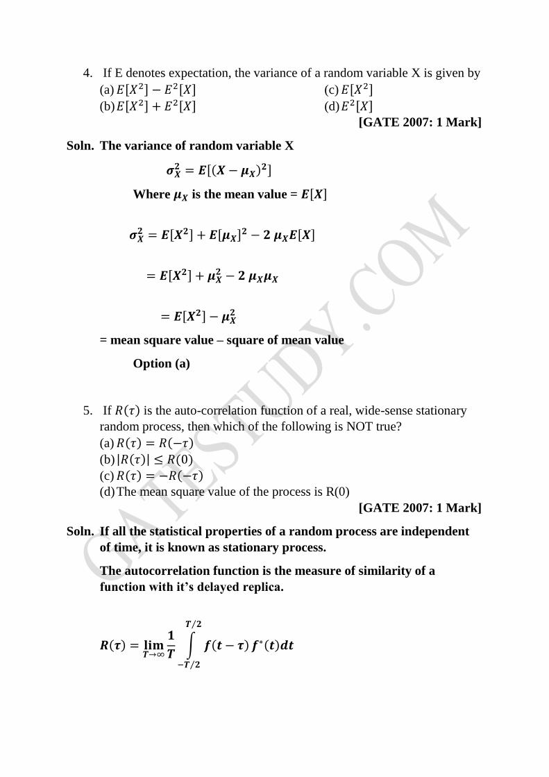
3. The distribution function 𝐹𝑋(𝑥) of a random variable X is shown in the
figure. The probability that X = 1 is
X-2 0 31
Fx(X)
0.25
0.55
1.0
(a) Zero
(b) 0.25
(c) 0.55
(d) 0.30
[GATE 2004: 1 Mark]
Soln. The probability that 𝑿 = 𝟏 = 𝑭𝑿(𝒙 = 𝟏+) − 𝑭𝑿(𝒙 = 𝟏−)
𝑷(𝒙 = 𝟏) = 𝟎. 𝟓𝟓 − 𝟎. 𝟐𝟓 = 𝟎. 𝟑𝟎
Option (d)
4. If E denotes expectation, the variance of a random variable X is given by
(a) 𝐸[𝑋2] − 𝐸2[𝑋]
(b) 𝐸[𝑋2] + 𝐸2[𝑋]
(c) 𝐸[𝑋2]
(d) 𝐸2[𝑋] [GATE 2007: 1 Mark]
Soln. The variance of random variable X
𝝈𝑿𝟐 = 𝑬[(𝑿 − 𝝁𝑿)𝟐]
Where 𝝁𝑿 is the mean value = 𝑬[𝑿]
𝝈𝑿𝟐 = 𝑬[𝑿𝟐] + 𝑬[𝝁𝑿]𝟐 − 𝟐 𝝁𝑿𝑬[𝑿]
= 𝑬[𝑿𝟐] + 𝝁𝑿𝟐 − 𝟐 𝝁𝑿𝝁𝑿
= 𝑬[𝑿𝟐] − 𝝁𝑿𝟐
= mean square value – square of mean value
Option (a)
5. If 𝑅(𝜏) is the auto-correlation function of a real, wide-sense stationary
random process, then which of the following is NOT true?
(a) 𝑅(𝜏) = 𝑅(−𝜏)
(b) |𝑅(𝜏)| ≤ 𝑅(0)
(c) 𝑅(𝜏) = −𝑅(−𝜏)
(d) The mean square value of the process is R(0)
[GATE 2007: 1 Mark]
Soln. If all the statistical properties of a random process are independent
of time, it is known as stationary process.
The autocorrelation function is the measure of similarity of a
function with it’s delayed replica.
𝑹(𝝉) = 𝐥𝐢𝐦𝑻→∞
𝟏
𝑻∫ 𝒇(𝒕 − 𝝉)
𝑻 𝟐⁄
−𝑻 𝟐⁄
𝒇∗(𝒕)𝒅𝒕
𝒇𝒐𝒓 𝝉 = 𝟎, 𝑹(𝟎) = 𝐥𝐢𝐦𝑻→∞
𝟏
𝑻∫ 𝒇(𝒕)
𝑻 𝟐⁄
−𝑻 𝟐⁄
𝒇∗(𝒕)𝒅𝒕
= 𝐥𝐢𝐦𝑻→∞
𝟏
𝑻∫ |𝒇(𝒕)|𝟐
𝑻 𝟐⁄
−𝑻 𝟐⁄
𝒅𝒕
R(0) is the average power P of the signal.
𝑹(𝝉) = 𝑹∗(−𝝉)𝒆𝒙𝒉𝒊𝒃𝒊𝒕𝒔 𝒄𝒐𝒏𝒋𝒖𝒈𝒂𝒕𝒆 𝒔𝒚𝒎𝒎𝒆𝒕𝒚
𝑹(𝝉) = 𝑹(−𝝉) 𝒇𝒐𝒓 𝒓𝒆𝒂𝒍 𝒇𝒖𝒏𝒄𝒕𝒊𝒐𝒏
𝑹(𝟎) ≥ 𝑹(𝝉) 𝒇𝒐𝒓 𝒂𝒍𝒍 𝝉
𝑹(𝝉) = −𝑹(−𝝉) is not true (since it has even symmetry)
Option (c)
6. If S(f) is the power spectral density of a real, wide-sense stationary
random process, then which of the following is ALWAYS true?
(a) 𝑆(0) ≥ 𝑆(𝑓)
(b) 𝑆(𝑓) ≥ 0
(c) 𝑆(−𝑓) = −𝑆(𝑓)
(d) ∫ 𝑆(𝑓)𝑑𝑓 = 0∞
−∞
[GATE 2007: 1 Mark]
Soln. Power spectral density is always positive
𝑺(𝒇) ≥ 𝟎
Option (b)
7. 𝑃𝑋(𝑥) = 𝑀 exp(−2|𝑥|) + 𝑁 𝑒𝑥𝑝(−3|𝑥|)is the probability density
function for the real random variable X over the entire X axis M and N
are both positive real numbers. The equation relating M and N is
(a) 𝑀 +2
3𝑁 = 1
(b) 2𝑀 +1
3𝑁 = 1
(c) 𝑀 + 𝑁 = 1
(d) 𝑀 + 𝑁 = 3
[GATE 2008: 2 Marks]
Soln.
∫ 𝑷𝑿(𝒙)
∞
−∞
𝒅𝒙 = 𝟏
∫(𝑴. 𝒆−𝟐𝒙 + 𝑵. 𝒆−𝟑𝒙)
∞
−∞
𝒅𝒙 = 𝟏
∫(𝑴. 𝒆−𝟐𝒙 + 𝑵. 𝒆−𝟑𝒙)
∞
𝟎
𝒅𝒙 =𝟏
𝟐
𝑴. 𝒆−𝟐𝒙
−𝟐|
𝟎
∞
+𝑵. 𝒆−𝟑𝒙
−𝟑|
𝟎
∞
=𝟏
𝟐
𝑴
𝟐+
𝑵
𝟑=
𝟏
𝟐
𝒐𝒓, 𝑴 +𝟐𝑵
𝟑= 𝟏
Option (a)
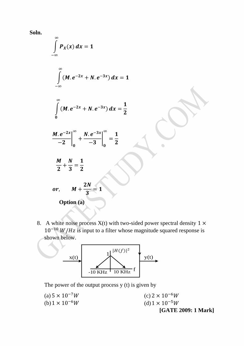
8. A white noise process X(t) with two-sided power spectral density 1 ×
10−10 𝑊/𝐻𝑧 is input to a filter whose magnitude squared response is
shown below.
x(t) y(t)
-10 KHz 10 KHzf
1
The power of the output process y (t) is given by
(a) 5 × 10⁻⁷𝑊
(b) 1 × 10⁻⁶𝑊
(c) 2 × 10⁻⁶𝑊
(d) 1 × 10⁻⁵𝑊
[GATE 2009: 1 Mark]
Soln. Power spectral density of white noise at the input of a filter = 𝑮𝒊(𝒇)
𝑮𝒊(𝒇) = 𝟏 × 𝟏𝟎−𝟏𝟎(𝑾/𝑯𝒛)
PSD at the output of a filter
𝑮𝟎(𝒇) = |𝑯(𝒇)|𝟐𝑮𝒊(𝒇)
=𝟏
𝟐(𝟐 × 𝟏𝟎 × 𝟏𝟎𝟑 × 𝟏) × 𝟏𝟎−𝟏𝟎
= 𝟏𝟎−𝟔𝑾
Option (b)
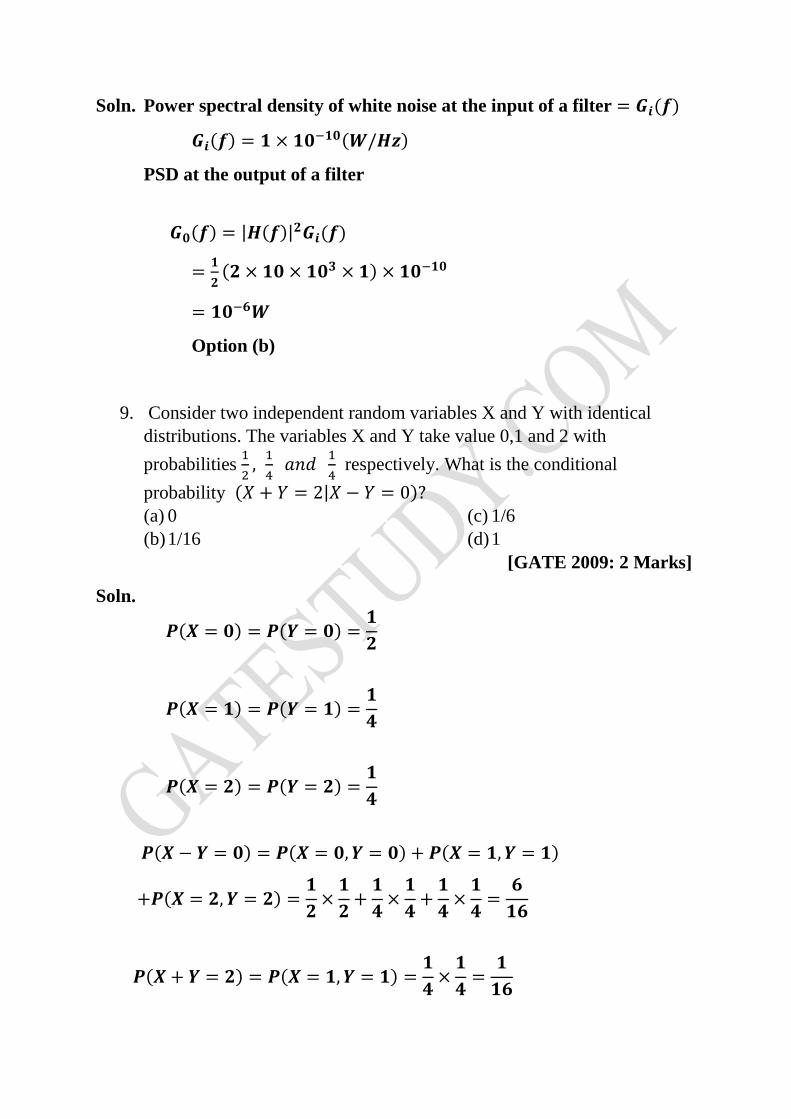
9. Consider two independent random variables X and Y with identical
distributions. The variables X and Y take value 0,1 and 2 with
probabilities 1
2,
1
4 𝑎𝑛𝑑
1
4 respectively. What is the conditional
probability (𝑋 + 𝑌 = 2|𝑋 − 𝑌 = 0)?
(a) 0
(b) 1/16
(c) 1/6
(d) 1
[GATE 2009: 2 Marks]
Soln.
𝑷(𝑿 = 𝟎) = 𝑷(𝒀 = 𝟎) =𝟏
𝟐
𝑷(𝑿 = 𝟏) = 𝑷(𝒀 = 𝟏) =𝟏
𝟒
𝑷(𝑿 = 𝟐) = 𝑷(𝒀 = 𝟐) =𝟏
𝟒
𝑷(𝑿 − 𝒀 = 𝟎) = 𝑷(𝑿 = 𝟎, 𝒀 = 𝟎) + 𝑷(𝑿 = 𝟏, 𝒀 = 𝟏)
+𝑷(𝑿 = 𝟐, 𝒀 = 𝟐) =𝟏
𝟐×
𝟏
𝟐+
𝟏
𝟒×
𝟏
𝟒+
𝟏
𝟒×
𝟏
𝟒=
𝟔
𝟏𝟔
𝑷(𝑿 + 𝒀 = 𝟐) = 𝑷(𝑿 = 𝟏, 𝒀 = 𝟏) =𝟏
𝟒×
𝟏
𝟒=
𝟏
𝟏𝟔
𝑷(𝑿 + 𝒀 = 𝟐 |𝑿−𝒀=𝟎) =𝟏
𝟏𝟔÷
𝟔
𝟏𝟔 =1/6
Option (c)
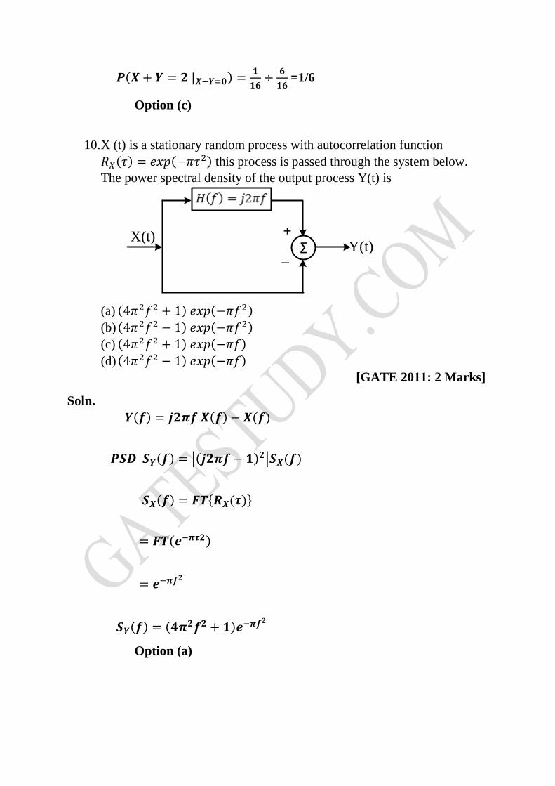
10. X (t) is a stationary random process with autocorrelation function
𝑅𝑋(𝜏) = 𝑒𝑥𝑝(−𝜋𝜏2) this process is passed through the system below.
The power spectral density of the output process Y(t) is
X(t) +
_Y(t)Σ
(a) (4𝜋2𝑓2 + 1) 𝑒𝑥𝑝(−𝜋𝑓2)
(b) (4𝜋2𝑓2 − 1) 𝑒𝑥𝑝(−𝜋𝑓2)
(c) (4𝜋2𝑓2 + 1) 𝑒𝑥𝑝(−𝜋𝑓)
(d) (4𝜋2𝑓2 − 1) 𝑒𝑥𝑝(−𝜋𝑓)
[GATE 2011: 2 Marks]
Soln.
𝒀(𝒇) = 𝒋𝟐𝝅𝒇 𝑿(𝒇) − 𝑿(𝒇)
𝑷𝑺𝑫 𝑺𝒀(𝒇) = |(𝒋𝟐𝝅𝒇 − 𝟏)𝟐|𝑺𝑿(𝒇)
𝑺𝑿(𝒇) = 𝑭𝑻{𝑹𝑿(𝝉)}
= 𝑭𝑻(𝒆−𝝅𝝉𝟐)
= 𝒆−𝝅𝒇𝟐
𝑺𝒀(𝒇) = (𝟒𝝅𝟐𝒇𝟐 + 𝟏)𝒆−𝝅𝒇𝟐
Option (a)
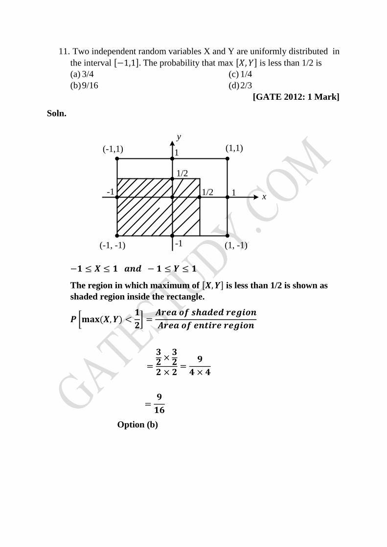
11. Two independent random variables X and Y are uniformly distributed in
the interval [−1,1]. The probability that max [𝑋, 𝑌] is less than 1/2 is
(a) 3/4
(b) 9/16
(c) 1/4
(d) 2/3
[GATE 2012: 1 Mark]
Soln.
(-1,1) (1,1)
(-1, -1) (1, -1)
-1 1
-1
1
x
y
1/2
1/2
−𝟏 ≤ 𝑿 ≤ 𝟏 𝒂𝒏𝒅 − 𝟏 ≤ 𝒀 ≤ 𝟏
The region in which maximum of [𝑿, 𝒀] is less than 1/2 is shown as
shaded region inside the rectangle.
𝑷 [𝐦𝐚𝐱 (𝑿, 𝒀) <𝟏
𝟐] =
𝑨𝒓𝒆𝒂 𝒐𝒇 𝒔𝒉𝒂𝒅𝒆𝒅 𝒓𝒆𝒈𝒊𝒐𝒏
𝑨𝒓𝒆𝒂 𝒐𝒇 𝒆𝒏𝒕𝒊𝒓𝒆 𝒓𝒆𝒈𝒊𝒐𝒏
=
𝟑𝟐
×𝟑𝟐
𝟐 × 𝟐=
𝟗
𝟒 × 𝟒
=𝟗
𝟏𝟔
Option (b)
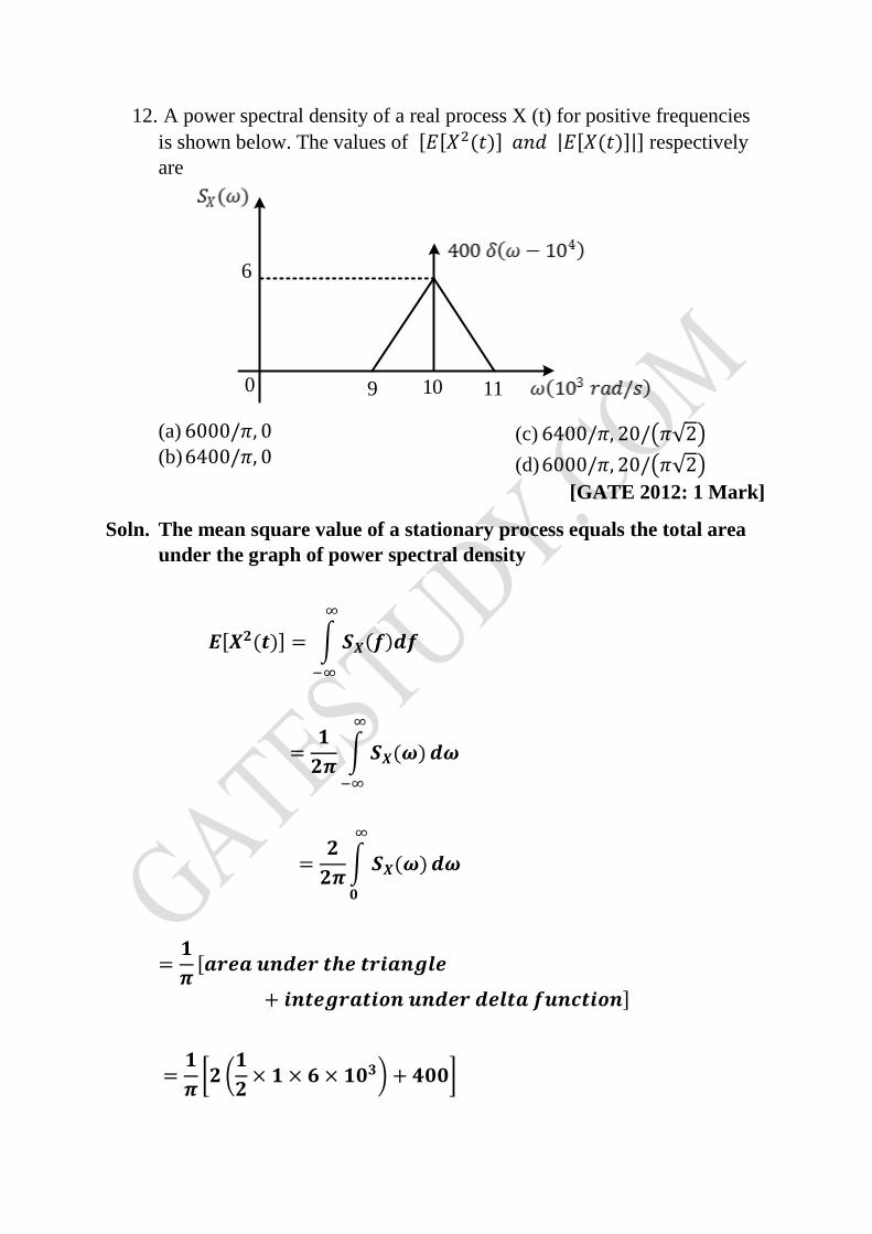
12. A power spectral density of a real process X (t) for positive frequencies
is shown below. The values of [𝐸[𝑋2(𝑡)] 𝑎𝑛𝑑 |𝐸[𝑋(𝑡)]|] respectively
are
0 10
6
9 11
(a) 6000/𝜋, 0
(b) 6400/𝜋, 0 (c) 6400/𝜋, 20/(𝜋√2)
(d) 6000/𝜋, 20/(𝜋√2)
[GATE 2012: 1 Mark]
Soln. The mean square value of a stationary process equals the total area
under the graph of power spectral density
𝑬[𝑿𝟐(𝒕)] = ∫ 𝑺𝑿(𝒇)𝒅𝒇
∞
−∞
=𝟏
𝟐𝝅∫ 𝑺𝑿(𝝎)
∞
−∞
𝒅𝝎
=𝟐
𝟐𝝅∫ 𝑺𝑿(𝝎)
∞
𝟎
𝒅𝝎
=𝟏
𝝅[𝒂𝒓𝒆𝒂 𝒖𝒏𝒅𝒆𝒓 𝒕𝒉𝒆 𝒕𝒓𝒊𝒂𝒏𝒈𝒍𝒆
+ 𝒊𝒏𝒕𝒆𝒈𝒓𝒂𝒕𝒊𝒐𝒏 𝒖𝒏𝒅𝒆𝒓 𝒅𝒆𝒍𝒕𝒂 𝒇𝒖𝒏𝒄𝒕𝒊𝒐𝒏]
=𝟏
𝝅[𝟐 (
𝟏
𝟐× 𝟏 × 𝟔 × 𝟏𝟎𝟑) + 𝟒𝟎𝟎]
=𝟔𝟒𝟎𝟎
𝝅
|𝑬[𝑿(𝒕)]| is the absolute value of mean of signal 𝑿(𝒕) which is also
equal to value of 𝑿(𝝎) at 𝝎 = 𝟎
From PSD
𝑺𝑿(𝝎)|𝝎=𝟎 = 𝟎
|𝑿(𝝎)|𝟐 = 𝟎
|𝑿(𝝎)| = 𝟎
Option (b)
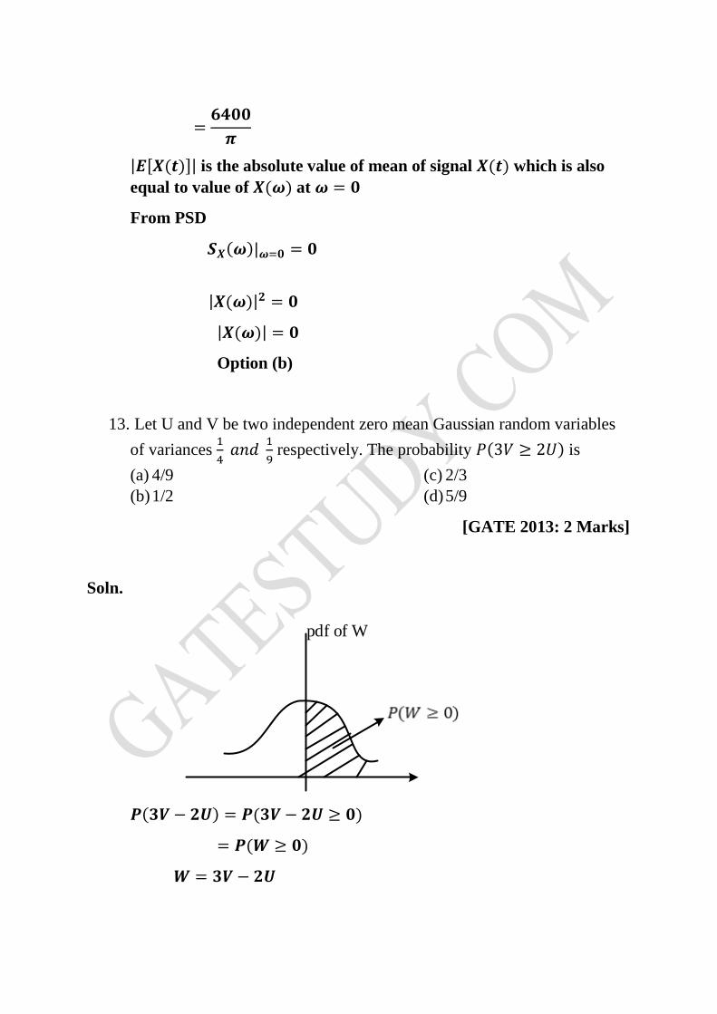
13. Let U and V be two independent zero mean Gaussian random variables
of variances 1
4 𝑎𝑛𝑑
1
9 respectively. The probability 𝑃(3𝑉 ≥ 2𝑈) is
(a) 4/9
(b) 1/2
(c) 2/3
(d) 5/9
[GATE 2013: 2 Marks]
Soln.
pdf of W
𝑷(𝟑𝑽 − 𝟐𝑼) = 𝑷(𝟑𝑽 − 𝟐𝑼 ≥ 𝟎)
= 𝑷(𝑾 ≥ 𝟎)
𝑾 = 𝟑𝑽 − 𝟐𝑼
W is the Gaussian Variable with zero mean having pdf curve as
shown below
𝑷(𝑾 ≥ 𝟎) =𝟏
𝟐(𝒂𝒓𝒆𝒂 𝒖𝒏𝒅𝒆𝒓 𝒕𝒉𝒆 𝒄𝒖𝒓𝒗𝒆 𝒇𝒓𝒐𝒎 𝟎 𝒕𝒐 ∞)
Option (b)
14. Let 𝑋1, 𝑋2, 𝑎𝑛𝑑 𝑋3 be independent and identically distributed random
variables with the uniform distribution on [0,1]. The probability
𝑃{𝑋1 𝑖𝑠 𝑡ℎ𝑒 𝑙𝑎𝑟𝑔𝑒𝑠𝑡} is ________
[GATE 2014: 1 Mark]
Soln. Probability 𝑷[𝑿𝟏] = 𝑷[𝑿𝟐] = 𝑷[𝑿𝟑]
𝑷𝟏 + 𝑷𝟐 + 𝑷𝟑 = 𝟏
𝑷(𝑿𝟏) + 𝑷(𝑿𝟐) + 𝑷(𝑿𝟑) = 𝟏
𝟑𝑷(𝑿𝟏) = 𝟏
𝑷(𝑿𝟏) =𝟏
𝟑
15. Let X be a real-valued random variable with 𝐸[𝑋] 𝑎𝑛𝑑 𝐸[𝑋2] denoting
the mean values of X and X2, respectively. The relation which always
holds
(a) (𝐸[𝑋])𝟐 > 𝐸[𝑋2]
(b) 𝐸[𝑋2] ≥ (𝐸[𝑋])𝟐
(c) 𝐸[𝑋2] = (𝐸[𝑋])2
(d) 𝐸[𝑋]2 > (𝐸[𝑋])2
[GATE 2014: 2 Marks]
Soln. variance 𝝈𝑿𝟐 = 𝑬[𝑿𝟐] − 𝒎𝑿
𝟐
𝑿𝟐̅̅̅̅ − 𝒎𝑿𝟐
= mean square value – square of mean value
𝝈𝑿𝟐 = 𝑬[𝑿𝟐] − [𝑬(𝑿)]𝟐
Variance is always positive so 𝑬[𝑿𝟐] ≥ [𝑬(𝑿)𝟐]
And can be zero
Option (b)
16. Consider a random process 𝑋(𝑡) = √2 sin(2𝜋𝑡 + 𝜙), where the random
phase ϕ is uniformly distributed in the interval[0,2𝜋]. The autocorrelation
𝐸[𝑋(𝑡1)𝑋(𝑡2)] is
(a) cos[2𝜋(𝑡1 + 𝑡2)]
(b) sin[2𝜋(𝑡1 − 𝑡2)]
(c) sin[2𝜋(𝑡1 + 𝑡2)]
(d) cos[2𝜋(𝑡1 − 𝑡2)] [GATE 2014: 2 Marks]
Soln. 𝑬[𝑿(𝒕𝟏) 𝑿(𝒕𝟐)] = 𝑬[𝑨 𝐬𝐢𝐧(𝟐𝝅𝒕𝟏 + 𝝓) × 𝑨 𝐬𝐢𝐧(𝟐𝝅𝒕𝟐 + 𝝓)]
=𝑨𝟐
𝟐𝑬[𝐜𝐨𝐬 𝟐𝝅(𝒕𝟏 − 𝒕𝟐) − 𝐜𝐨𝐬 𝟐𝝅(𝒕𝟏 + 𝒕𝟐 + 𝟐𝝓)]
=𝑨𝟐
𝟐𝐜𝐨𝐬 𝟐𝝅(𝒕𝟏 − 𝒕𝟐)
𝑬[𝐜𝐨𝐬 𝟐𝝅(𝒕𝟏 + 𝒕𝟐 + 𝟐𝝓)] = 𝟎
Option (d)
17. Let X be a random variable which is uniformly chosen from the set of
positive odd numbers less than 100. The expectation, E[X] is
[GATE 2014: 1 Mark]
Soln.
𝑬[𝑿] =𝟏 + 𝟑 + 𝟓 + − − − − (𝟐𝒏 − 𝟏)
𝟓𝟎
Where n = 50
=𝒏𝟐
𝟓𝟎= 𝟓𝟎
18. The input to a 1-bit quantizer is a random variable X with pdf 𝑓𝑋(𝑥) =
2𝑒−2𝑥 𝑓𝑜𝑟 𝑥 ≥ 0 and𝑓𝑋(𝑥) = 0 𝑓𝑜𝑟 𝑥 < 0. For outputs to be of equal
probability, the quantizer threshold should be______
[GATE 2014: 2 Marks]
Soln. The input to a 1-bit quantizer is a random variable X with pdf
𝒇𝑿(𝒙) = 𝟐𝒆−𝟐𝒙 𝒇𝒐𝒓 𝒙 ≥ 𝟎 And 𝒇𝑿(𝒙) = 𝟎 𝒇𝒐𝒓 𝒙 < 𝟎 let Vthr be the
quantizer threshold
∫ 𝟐𝒆−𝟐𝒙
𝑽𝒕𝒉𝒓
−∞
𝒅𝒙 = ∫ 𝟐𝒆−𝟐𝒙
∞
𝑽𝒕𝒉𝒓
𝒅𝒙
= ∫ 𝟐𝒆−𝟐𝒙
𝑽𝒕𝒉𝒓
𝟎
𝒅𝒙 = ∫ 𝟐𝒆−𝟐𝒙
∞
𝑽𝒕𝒉𝒓
𝒅𝒙 𝒇𝑿(𝒙) = 𝟎 𝒇𝒐𝒓 𝒙 < 𝟎
𝟐𝒆−𝟐𝒙
−𝟐|
𝟎
𝑽𝒕𝒉𝒓
=𝟐𝒆−𝟐𝒙
−𝟐|
𝑽𝒕𝒉𝒓
∞
(−𝒆−𝟐𝑽𝒕𝒉𝒓 + 𝒆−𝟎) = −(𝟎 − 𝒆−𝟐𝑽𝒕𝒉𝒓)
𝒆−𝟐𝑽𝒕𝒉𝒓 =𝟏
𝟐
−𝟐𝑽𝒕𝒉𝒓 = 𝒍𝒏 (𝟏
𝟐) = (−𝟎. 𝟔𝟗𝟑)
𝑽𝒕𝒉𝒓 =𝟎. 𝟔𝟗𝟑
𝟐
= 0.346


