Download - Principles and Instruments of Diagnostic Ultrasound

This chapter is an April 2005 revision of a chapter writtenin April 1998. During that period, the basics of ultrasoundexamination have been surprisingly stable. Electronicshave shrunk so that now full function ultrasound duplexscanners can fit in your pocket. The speed of personalcomputers has advanced so that the new scanners are justsoftware residing in personal computers equipped withan ultrasound receiver on the front end and a printer orDICOM adaptor on the back end.

In spite of shrinking electronics, all of the “modern”triplex-Doppler, color flow, (three-dimensional real-time)“four-dimensional” scanners have converged on a singlestandard package. Most instruments are still 20 inches (50cm) wide, 30 inches (75cm) long, and 50 inches (125cm) tall, with a power cord that requires 120V (240V in Europe), 60Hz (50Hz in Europe), delivering amaximum of 15 A (7.5 A in Europe) or 1800W (volts multiplied by amps) with a printer included.This standardwas developed because doorways are 30 inches (760mm)wide and the eyes of ultrasound examiners are located 60 inches (150cm) off the ground, and power outlets are ubiquitous. This way, an examiner can roll the ultrasound instrument through a door while the exam-iner’s view over the top of the instrument is unobstructedand connect the instrument to power at the patient’sbedside. Thus the systems are “portable,” something thatwill always be out of reach of the computed tomography(CT) and magnetic resonance imaging (MRI) alternativetechnologies. It is truly surprising that the manufacturers,over the period from 1979 (when commercial duplexscanners became popular) to 2005, while electronics haveshrunk to (1/2)18 or 1/250,000 size, have elected to keepthe instrument package unchanged until this year with theintroduction of notebook size systems. What has changedis that the complexity of the systems has exploded. Nowultrasound scanners are over 4000 times as complex as in 1979. But, that era has come to an end. The first companies to introduce palm size scanners have revertedto mounting them on standard size carts, not because

small size is impossible, but because the customers appearto want ultrasound scanners that look large. Now, all themajor manufacturers offer palm size ultrasound scannersas an alternative to the large systems.

This chapter was written in the United States in a worldwhere inches and feet, gallons and quarts are the rule,and room temperature is 72°F (22°C) and body tempera-ture is 98.6°F (37°C). “Science” has “advanced” to use adecimal metric system. The decimal system, however, ismisaligned with the computer-friendly binary numbersystem. As an example, 0.1 is an irrational number inbinary computer math. In the future, I predict, the decimalsystem will be discarded in favor of a binary (or hexa-decimal) system that is more compatible with computers.In the meantime, the relationship between the decimaland binary systems will require constant explanation.

In this chapter, the MKS (meter kilogram second)system will be used when alternatives are not more con-venient.To facilitate understanding, all units will be listedevery time a number is given. To make things more diffi-cult, the “scientists” have decided to honor their own bynaming often used groups of units after the great peoplein physics, like Hertz for frequency instead of cycles persecond, Pascals for pressure instead of Newton persquare meter, and Rayls for impedance instead of kilo-grams per square meter per second. In this chapter, alongwith the modern names, the more primitive units ofmeasure will be included in order to foster the ability ofthe reader to correctly perform important computations,which facilitate the understanding of future instrumentsand methods. The results of many computations are quiteastounding.

Introduction

Medical imaging of the body requires the completion ofthree tasks: (1) locating volumes of tissue in the body(voxels) to be examined, (2) measuring one or more

3Principles and Instruments of DiagnosticUltrasound and Doppler UltrasoundKirk W. Beach, Marla Paun, and Jean F. Primozich

11

12 K.W. Beach et al.

feature(s) of the tissue within each volume, and (3) deliv-ering the data to the brain of the examiner/interpreter.The primary sensory channel used in medical imaging is the retina, a two-dimensional, analog/trichromatic(color), cine-capable (motion) data path. A secondarychannel used exclusively in ultrasound Doppler is dual audio channels (two ears). Although used in physi-cal examination, the tactile, taste, and olfactory senses are not currently used in medical imaging. A two-dimensional medical image presentation involves twotasks: (1) arranging areas on a screen (pixels) that corre-spond to tissue voxels and (2) displaying the measure-ment from the corresponding tissue voxel in each pixel.If more than one measurement type is made from eachvoxel (for example, echogenicity and tissue velocity) then both data types can be shown in a single pixel onthe screen by differentiating the echogenicity (shown in gray scale) from the velocity (shown in colors) by usingthe trivariable (red-green-blue) nature of the eye. If the process is done once to form one image, the image is called “static”; if the process is repeated rapidly (10 or more times per second) to show motion, then theprocess may be called “real time.” These steps arerequired in all sectional imaging modalities such as CT,MRI, positron emission tomography (PET) imaging,and ultrasound. Note that the voxels used in sectionalimaging are different from the voxels used in projectionalimaging like conventional X-ray and nuclear imaging.In sectional imaging, the voxels are nearly cubic, whereasin projectional imaging the voxels are long rods pene-trating the entire body and viewed from the end as pixels(dots).

In the following discussion, ultrasonic imaging consistsof three steps: (1) the voxels will be located, (2) meas-urements on each tissue voxel will be made, and (3) thetissue data from each voxel in the image plane will be dis-played as a two-dimensional array of pixels. This discus-sion will be limited to pulse echo ultrasound; continuouswave ultrasound will not be covered. There are severalalternatives to the popular methods that may becomeuseful in the future.

Locating Voxels with Pulse Echo Ultrasound

A transmitting ultrasound transducer is designed todirect a pulse of ultrasound along a needle-like beampattern from the transducer through the body tissues.Voxels located along that beam pattern provide echoesthat return to the receiving transducer along a needle-like beam pattern. Usually the transmitting transduceraperture and the receiving transducer aperture are at thesame location, so the transmit beam path and the receive

beam path are the same. The location of each voxelreflecting ultrasound from along the beam can be deter-mined by the time taken for the echo to return. Data froma reflector at a depth of 1cm returns to the transducer in13µs; data from a depth of 3cm returns in 40µs; data from15cm returns in 200µs. Except for the details, this is acomplete description of pulse-echo ultrasound.To under-stand the physics and consequences on the image in moredetail, we need to separate four coordinate directions intissue: (1) distance from the ultrasound transducer(depth), (2) lateral direction in the image (ultrasoundbeam pattern width), (3) thickness direction in the image(ultrasound beam pattern thickness), and (4) time ofimage acquisition (frame interval/sweep) in the cardiaccycle. The physics of each of these is different. Thus, eachof these has an associated resolution. We will considereach of these in sequence.

Distance from the Ultrasound Transducer Depth

Pulse-echo ultrasound involves transmitting a short pulseof ultrasound into tissue and then receiving the echoesthat return from the tissues located at each depth alongthe ultrasound beam pattern.The echo time, the time aftertransmission for an echo to return from a voxel at a par-ticular depth, can be computed from the speed of ultra-sound in tissue. The speed of ultrasound in tissue is calledC. In most body tissues C is about 1500 (± 80) m/s =150,000cm/s = 1.5mm/µs.

To compute the time [t] required for an echo to returnfrom a voxel at a particular depth [d], the round trip dis-tance of travel must be used [t = 2d/C]. For an echo toreturn from a depth of 3cm (30mm), the time requiredis [t = 2 ∗ 30mm/1.5mm/µs = 40µs]. The result of thiscomputation for a series of depths is given in Table 3–1.

In a typical ultrasound machine, the time when echoesare returning is divided into 200 divisions, each divisionbeing 1µs long. Each division takes data from a 0.75-mmvoxel along the ultrasound beam pattern to provide datafor a pixel along the beam line on the screen. Each beamline on the screen is thin and straight corresponding tothe thin straight ultrasound transmit beam pattern andthin straight ultrasound receive beam pattern. Most ultra-

Table 3–1. Ultrasound echo time for depth.

Depth Time Vessel

0.75mm 1µs1.5mm 2µs Finger artery

15mm 20µs Superficial vein3cm 40µs Carotid artery9cm 120µs Renal artery

15cm 200 µs

3. Principles and Instruments of Diagnostic Ultrasound and Doppler Ultrasound 13

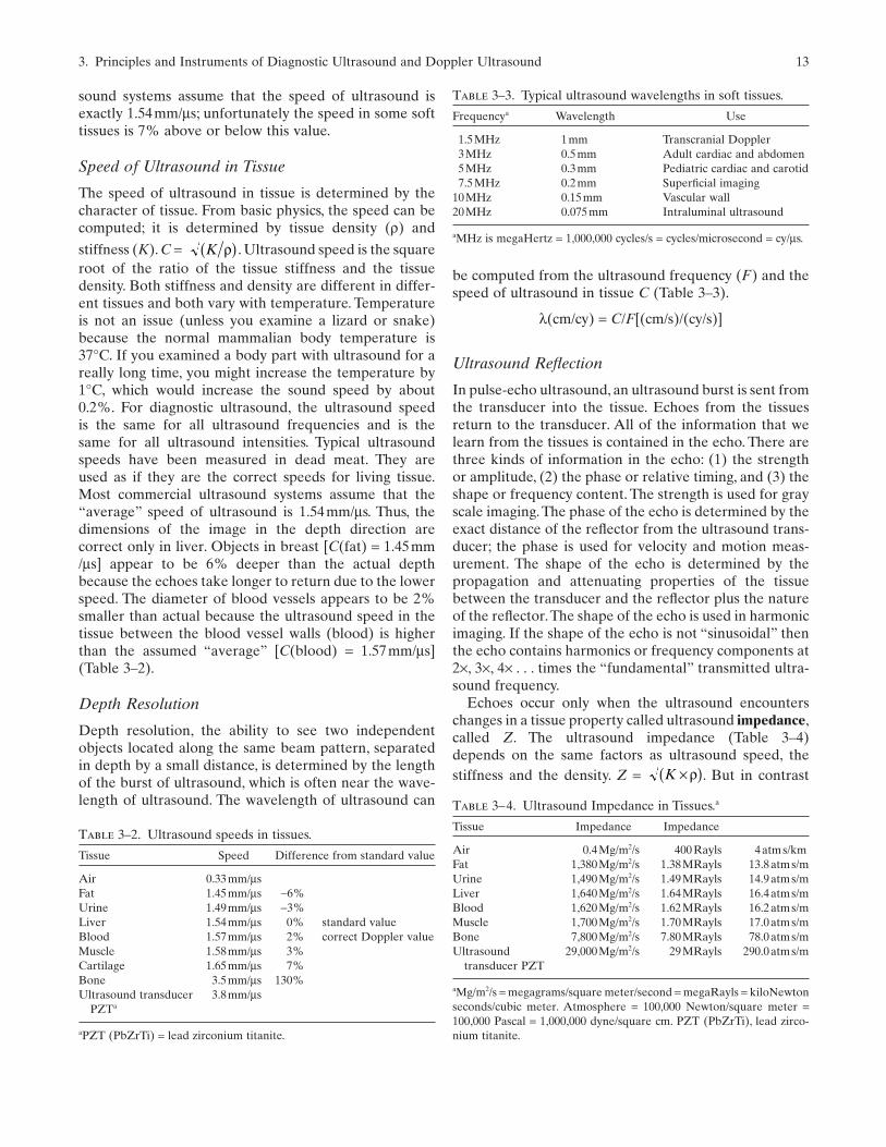
sound systems assume that the speed of ultrasound isexactly 1.54mm/µs; unfortunately the speed in some softtissues is 7% above or below this value.

Speed of Ultrasound in Tissue

The speed of ultrasound in tissue is determined by thecharacter of tissue. From basic physics, the speed can becomputed; it is determined by tissue density (ρ) and

stiffness (K). C = . Ultrasound speed is the squareroot of the ratio of the tissue stiffness and the tissuedensity. Both stiffness and density are different in differ-ent tissues and both vary with temperature. Temperatureis not an issue (unless you examine a lizard or snake)because the normal mammalian body temperature is37°C. If you examined a body part with ultrasound for areally long time, you might increase the temperature by1°C, which would increase the sound speed by about0.2%. For diagnostic ultrasound, the ultrasound speed is the same for all ultrasound frequencies and is the same for all ultrasound intensities. Typical ultrasoundspeeds have been measured in dead meat. They are used as if they are the correct speeds for living tissue.Most commercial ultrasound systems assume that the“average” speed of ultrasound is 1.54mm/µs. Thus, thedimensions of the image in the depth direction arecorrect only in liver. Objects in breast [C(fat) = 1.45mm/µs] appear to be 6% deeper than the actual depthbecause the echoes take longer to return due to the lowerspeed. The diameter of blood vessels appears to be 2%smaller than actual because the ultrasound speed in thetissue between the blood vessel walls (blood) is higherthan the assumed “average” [C(blood) = 1.57mm/µs](Table 3–2).

Depth Resolution

Depth resolution, the ability to see two independentobjects located along the same beam pattern, separatedin depth by a small distance, is determined by the lengthof the burst of ultrasound, which is often near the wave-length of ultrasound. The wavelength of ultrasound can

K ρ( )be computed from the ultrasound frequency (F) and thespeed of ultrasound in tissue C (Table 3–3).

λ(cm/cy) = C/F[(cm/s)/(cy/s)]

Ultrasound Reflection

In pulse-echo ultrasound, an ultrasound burst is sent fromthe transducer into the tissue. Echoes from the tissuesreturn to the transducer. All of the information that welearn from the tissues is contained in the echo. There arethree kinds of information in the echo: (1) the strengthor amplitude, (2) the phase or relative timing, and (3) theshape or frequency content. The strength is used for grayscale imaging.The phase of the echo is determined by theexact distance of the reflector from the ultrasound trans-ducer; the phase is used for velocity and motion meas-urement. The shape of the echo is determined by thepropagation and attenuating properties of the tissuebetween the transducer and the reflector plus the natureof the reflector.The shape of the echo is used in harmonicimaging. If the shape of the echo is not “sinusoidal” thenthe echo contains harmonics or frequency components at2×, 3×, 4× . . . times the “fundamental” transmitted ultra-sound frequency.

Echoes occur only when the ultrasound encounterschanges in a tissue property called ultrasound impedance,called Z. The ultrasound impedance (Table 3–4) depends on the same factors as ultrasound speed, the stiffness and the density. Z = . But in contrast K ×( )ρ

Table 3–2. Ultrasound speeds in tissues.

Tissue Speed Difference from standard value

Air 0.33mm/µsFat 1.45mm/µs −6%Urine 1.49mm/µs −3%Liver 1.54mm/µs 0% standard valueBlood 1.57mm/µs 2% correct Doppler valueMuscle 1.58mm/µs 3%Cartilage 1.65mm/µs 7%Bone 3.5mm/µs 130%Ultrasound transducer 3.8mm/µs

PZTa

aPZT (PbZrTi) = lead zirconium titanite.

Table 3–3. Typical ultrasound wavelengths in soft tissues.

Frequencya Wavelength Use

1.5MHz 1mm Transcranial Doppler3MHz 0.5mm Adult cardiac and abdomen5MHz 0.3mm Pediatric cardiac and carotid7.5MHz 0.2mm Superficial imaging

10MHz 0.15mm Vascular wall20MHz 0.075mm Intraluminal ultrasound

aMHz is megaHertz = 1,000,000 cycles/s = cycles/microsecond = cy/µs.

Table 3–4. Ultrasound Impedance in Tissues.a

Tissue Impedance Impedance

Air 0.4Mg/m2/s 400Rayls 4atms/kmFat 1,380Mg/m2/s 1.38MRayls 13.8atms/mUrine 1,490Mg/m2/s 1.49MRayls 14.9atms/mLiver 1,640Mg/m2/s 1.64MRayls 16.4atms/mBlood 1,620Mg/m2/s 1.62MRayls 16.2atms/mMuscle 1,700Mg/m2/s 1.70MRayls 17.0atms/mBone 7,800Mg/m2/s 7.80MRayls 78.0atms/mUltrasound 29,000Mg/m2/s 29MRayls 290.0atms/m

transducer PZT

aMg/m2/s = megagrams/square meter/second = megaRayls = kiloNewtonseconds/cubic meter. Atmosphere = 100,000 Newton/square meter =100,000 Pascal = 1,000,000 dyne/square cm. PZT (PbZrTi), lead zirco-nium titanite.


to ultrasound speed, ultrasound impedance is the squareroot of the product of the tissue stiffness and the tissuedensity.

Rayl =kg/m2/s

Some authors prefer to express impedance as the productof tissue density and ultrasound speed. With algebra, youcan demonstrate that these are the same.

The difference in impedance between the superficialtissue and the deep tissue at an interface determines thestrength of the reflector and therefore is proportional tothe amplitude of the ultrasound echo. R = (Z2 − Z1)/(Z2 + Z1). If the difference between the impedances isgreater, then the fraction of the incident ultrasound thatis reflected is larger. The pulse energy is proportional tothe square of the amplitude, so the energy reflected isequal to R2. Table 3–5 shows that the reflected energyfrom an ultrasound pulse as it crosses an interfacebetween two soft tissues is usually less than 1%. Reflec-tions at the surface of bone interfaces are near 50%.Reflections at the surface of air interfaces are greaterthan 99%. The greatest reflections between solids occurat the surface of a PZT (PbZrTi, lead zirconium titanite)ultrasound transducer. Less than 0.12% of the energy inthe transducer will pass into tissue in an ultrasound cycle;less than 0.01% will pass from the transducer into air.

As ultrasound passes from fat into muscle, 1% of theultrasound pulse energy is reflected and 99% is trans-mitted. The same percentage is reflected as ultrasoundpasses from muscle into fat. However, as shown in Table3–6, there is a difference between the two reflections. Asultrasound is passing from muscle to fat, the shape of thereflected pulse is inverted because the distal tissue has alower impedance than the proximal tissue; the inversionis indicated by the minus sign in Table 3–6.

Ultrasound Attenuation

As an ultrasound pulse travels through tissue, the energyin the pulse decreases. Some of the energy is reflected byinterfaces and scatterers where the impedance changes,some of the energy is absorbed by the tissue causing thetissue to heat, and some of the energy is converted intoharmonic ultrasound frequencies that are not received bythe ultrasound system. For imaging purposes, the impor-tance of attenuation is that the strength of the echoesreceived from deep tissues is less than the strength of theechoes from similar superficial tissues. This complicatesthe interpretation of echo strength. The time gain control(TGC) should be set to compensate for the attenuation.This control is also called depth gain compensation(DGC), system time compensation (STC), and othernames.

Table 3–5. Ultrasound energy reflection at different interfaces between materials.

Impedance Air Fat Urine Blood Liver Muscle BoneTissue MRayls 0.0004 1.38 1.49 1.62 1.64 1.7 7.8

Air 0.0004Fat 1.38 99.88%Urine 1.49 99.89% 0.15%Blood 1.62 99.90% 0.64% 0.17%Liver 1.64 99.90% 0.74% 0.23% 0.00%Muscle 1.7 99.91% 1.08% 0.43% 0.06% 0.03%Bone 7.8 99.98% 48.91% 46.13% 43.04% 42.58% 41.23%PZTa 29 99.99% 82.66% 81.41% 79.96% 79.74% 79.08% 33.19%

aPZT (PbZrTi), lead zirconium titanite.

Table 3–6. Ultrasound amplitude reflection at different interfaces between materials.

Material on the superficial side of the interface

Impedance Air Fat Urine Blood Liver Muscle Bone PZTa

Tissue Mrayls 0.0004 1.38 1.49 1.62 1.64 1.7 7.8 29

Air 0.0004 0 −0.99942 −0.99946 −0.99951 −0.99951 −0.99953 −0.99990 −0.99997Fat 1.38 0.99942 0 −0.03833 −0.08000 −0.08609 −0.10390 −0.69935 −0.90915Urine 1.49 0.99946 0.03833 0 −0.04180 −0.04792 −0.06583 −0.67922 −0.90226Blood 1.62 0.99951 0.08000 0.04180 0 −0.00613 −0.02410 −0.65605 −0.89419Liver 1.64 0.99951 0.08609 0.04792 0.00613 0 −0.01796 −0.65254 −0.89295Muscle 1.7 0.99953 0.10390 0.06583 0.02410 0.01796 0 −0.64211 −0.88925Bone 7.8 0.99990 0.69935 0.67922 0.65605 0.65254 0.64211 0 −0.57609PZT 29 0.99997 0.90915 0.90226 0.89419 0.89295 0.88925 0.57609 0

aPZT (PbZrTi), lead zirconium titanite.


The effect of attenuation on the strength of the echoreceived from a voxel can be computed using the atten-uation rate and thickness of the tissues between the ultra-sound transducer and the voxel. The attenuation rate isexpressed in three different kinds of units: Nepers, deci-bels, and half-thickness.

As a 1-MHz ultrasound pulse passes through a sectionof typical soft tissue 10cm thick, approximately 90% ofthe energy is reflected (scattered), absorbed (convertedto heat), or converted to harmonics, so only 10% of theoriginal energy is present in the pulse leaving the section.Attenuation to 0.1 of the original pulse energy is called1 bel (B) of attenuation. If the ultrasound passes throughan additional 10-cm-thick section, only 0.1 of the previ-ous 0.1 or 0.01 of the original energy survives. This iscalled 2B of attenuation. If ultrasound passes through 30cm of soft tissue, only 0.001 (0.13) of the original pulseenergy survives. This is called 3B of attenuation. Theseunits are too large for the engineers that use them so theyuse decibels: 10dB is equal to 1B.

As a 1-MHz ultrasound pulse passes through a sectionof typical soft tissue 3cm thick, approximately 50% of theenergy is reflected (scattered) or absorbed (converted toheat), so 50% of the original energy is present in the pulseleaving the section. Thus, 3cm is the half value thicknessor half value layer. If the ultrasound passes through 3 halfvalue layers or 9cm, then (0.5 × 0.5 × 0.5) 0.125 of theenergy in the pulse survives. If the ultrasound passesthrough 30cm or 10 half value layers, then (0.510) 0.001 ofthe original energy is still in the pulse. Fortunately, theanswer is the same for 30cm of tissue whether computedin decibels or in half value layers.

If Ef is the surviving energy and Eo is the incidentenergy, then

Ef/Eo = 0.1d/10 = 0.5H

where d is in decibels and H is in half value layers.If the ultrasound frequency is doubled, the attenuation

for each centimeter is doubled.The attenuation per ultra-sound cycle is constant over wide ranges. A half valuelayer of soft tissue is about 20 wavelengths thick. A tissuelayer that attenuates ultrasound by 10dB is 67 wave-lengths. The attenuation rate in some soft tissues isgreater than in others.

The attenuation refers to energy or power, but not tointensity. Power is energy/time; intensity is power/area.As ultrasound spreads or converges, the area of the beamchanges. Changes in intensity are due to a combinationof changes in power and changes in area. In turn, pres-sure amplitude is dependent on intensity. Attenuation inNepers is defined as If/Io = exp(− η) where η is the atten-uation in Nepers. This would be acceptable if the beamdid not diverge or converge so that the beam cross-sectional area did not change. In that case d = 3 × H =8.69 × η.

Attenuation in some tissues is greater than in othertissues (Table 3–7).

Ultrasound Intensity

The meaning of ultrasound impedance is not as obviousas the meaning of ultrasound speed. To understandimpedance, imagine what happens as ultrasound passesthrough tissue. As the ultrasound wave travels through a portion of tissue, the molecules in that portion of the tissue jiggle in the wave propagation direction, inresponse to pressure changes in the forward and back-ward direction as the wave passes. Since the molecularmotion is in the same direction as the wave travels, this iscalled a longitudinal wave. Ultrasound impedance is theratio of the pressure fluctuation (p) to the molecularvelocity fluctuation (v) as the wave passes Z = p/v. Theinstantaneous intensity of the wave is the product of thepressure fluctuation and the velocity fluctuation. i = p × v.P, the instantaneous air pressure, includes two parts, theatmospheric pressure A and the fluctuating part p, P =A + p. With algebra, you can show that i = Z × v2 or that i = p2/Z. Typical medical ultrasound values are shown inTable 3–8.

For continuous wave (CW) ultrasound, a continuoussound wave that can be expressed as a sine wave, theaverage intensity I can be computed.

Table 3–7. Ultrasound attenuation in tissues.a

Tissue Cycles/decibel Cycles/half thickness Cycles/Neper

Urine 1000 3010 8690Blood 37 111 321Fat 11 33 95.6Liver 7 21 60.8Muscle 3 9 38.7

aFor a nonconverging beam.

Table 3–8. Ultrasound intensity wave parameters in soft tissueif Z = 1.5MRayls.

Molecular velocityIntensitya Pressure fluctuations fluctuations

10mW/cm2 17kN/m2 = 0.17atm 1.2cm/s100mW/cm2 b 54kN/m2 = 0.54atm 3.6cm/s333mW/cm2 100kN/m2 = 1.00atmc 6.6cm/s

1,000mW/cm2 170kN/m2 = 1.70atm 11.5cm/s3,000mW/cm2 d 295kN/m2 = 2.95atm 20cm/s

10,000mW/cm2 e 540kN/m2 = 5.40atm 36.4cm/s2,000W/cm2 f 7.6MN/m2 = 76atm 510cm/s

aIntensity refers to spatial peak temporal peak for pulsed ultrasound.bMaximum “continuous wave” intensity for diagnostic ultrasound.cPressure fluctuaftion equals 1 atmosphere.dTypical continuous wave intensity used for therapeutic ultrasound.eSpatial peak temporal peak intensity typical of diagnostic ultrasound.fHigh intensity focused ultrasound cautery.


or

pm =

and similarly

vm =

Note that the relationships between intensity, the pres-sure fluctuations, and the molecular velocity fluctuationsare independent of ultrasound frequency. Each dependson the ultrasound intensity and the tissue impedance.

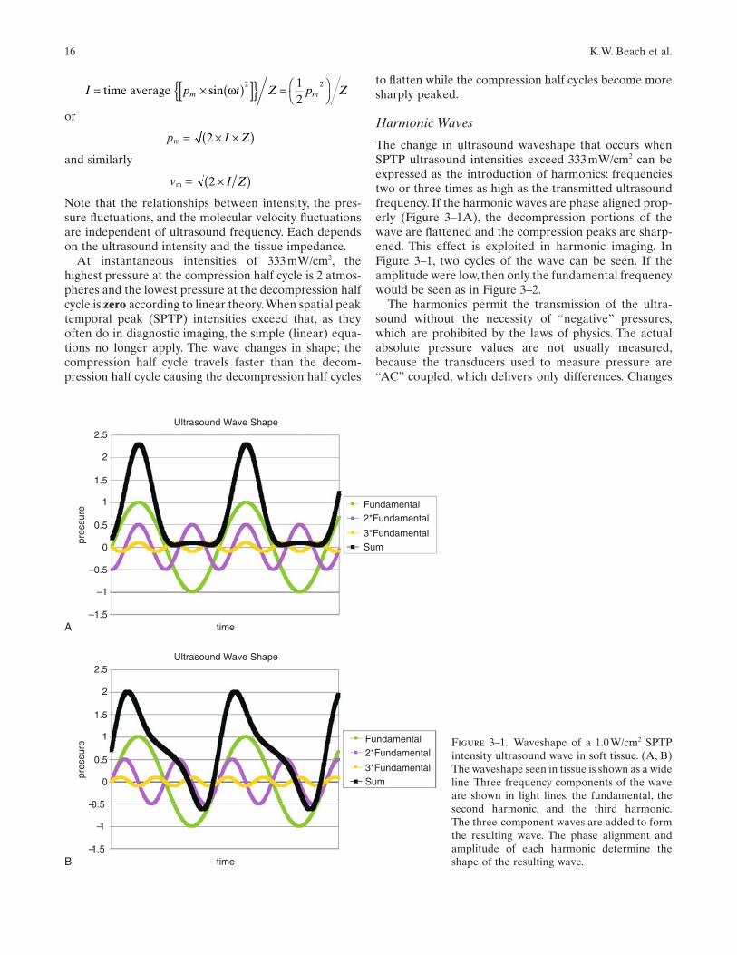
At instantaneous intensities of 333mW/cm2, thehighest pressure at the compression half cycle is 2 atmos-pheres and the lowest pressure at the decompression halfcycle is zero according to linear theory.When spatial peaktemporal peak (SPTP) intensities exceed that, as theyoften do in diagnostic imaging, the simple (linear) equa-tions no longer apply. The wave changes in shape; thecompression half cycle travels faster than the decom-pression half cycle causing the decompression half cycles

2 ×( )I Z

2 × ×( )I Z

I p t Z p Zm m= × ( )[ ]{ } = ⎛⎝

⎞⎠time average sin ω 2 21

2

to flatten while the compression half cycles become moresharply peaked.

Harmonic Waves

The change in ultrasound waveshape that occurs whenSPTP ultrasound intensities exceed 333mW/cm2 can beexpressed as the introduction of harmonics: frequenciestwo or three times as high as the transmitted ultrasoundfrequency. If the harmonic waves are phase aligned prop-erly (Figure 3–1A), the decompression portions of thewave are flattened and the compression peaks are sharp-ened. This effect is exploited in harmonic imaging. InFigure 3–1, two cycles of the wave can be seen. If theamplitude were low, then only the fundamental frequencywould be seen as in Figure 3–2.

The harmonics permit the transmission of the ultra-sound without the necessity of “negative” pressures,which are prohibited by the laws of physics. The actualabsolute pressure values are not usually measured,because the transducers used to measure pressure are“AC” coupled, which delivers only differences. Changes

Ultrasound Wave Shape

Fundamental2*Fundamental

3*FundamentalSum

2.5

2

1.5

1

0.5

0

–0.5

–1

–1.5timeA

pres

sure

Figure 3–1. Waveshape of a 1.0W/cm2 SPTPintensity ultrasound wave in soft tissue. (A, B)The waveshape seen in tissue is shown as a wideline. Three frequency components of the waveare shown in light lines, the fundamental, thesecond harmonic, and the third harmonic.The three-component waves are added to formthe resulting wave. The phase alignment andamplitude of each harmonic determine theshape of the resulting wave.

Ultrasound Wave Shape

Fundamental2*Fundamental

3*FundamentalSum

2.5

2

1.5

1

0.5

0

–0.5

–1

–1.5timeB

pres

sure


in wave speed at extreme pressures can alter the wave-shape (Figure 3–1B). George Keilman has shown that afocused ultrasound beam that forms peaks like those inFigure 3–1 will revert to a sinusoid like Figure 3–2 ifreflected by an inverting reflector in the middle of thepath (Z2 < Z1), but will convert more energy to harmon-ics if reflected by a noninverting reflector in the middleof the path (Z2 > Z1).

Harmonics are also formed when ultrasound interactswith bubbles in the ultrasound beam. The history ofbubbles and harmonic imaging is interesting. Ultrasoundcontrast made by agitating saline has been used for yearsby cardiologists to diagnose patent foramen ovale (PFO).Injected intravenously, the microbubbles are too large topass through the lung.They are very echogenic in the ven-tricle. If they appear in the left ventricle, a PFO is diag-nosed. Recently ultrasound contrast agents consisting ofbubbles smaller than 8µm in size (the size of an erythro-cyte) have been manufactured so that they will passthrough the capillaries of the lung. When injected intra-venously, these will permit ultrasound contrast studies inarteries and organs supplied by the systemic arterial circulation.

Usually, small bubbles are not stable in liquid becausethe surface tension at the interface between the gas andthe liquid squeezes the bubbles and causes the gas to dis-solve.The surface tension can be reduced by adding a sur-factant that acts like soap. Common surfactants includealbumen and sugars. Of course, the chemical propertiesof the surfactant can be used to cause the bubbles toattach to the endothelial surface of blood vessels. Ratherthan a bubble filled with air, which has a moderate solu-bility in water (which shortens the life of the contrastagent in blood), contrast bubbles often contain fluoro-carbons that have poor solubility in water and bloodplasma. This increases the duration of bubble survival in

the tissues. The fluorocarbons do have a high solubility infat, a factor that has not yet been explored in ultrasoundcontrast agents.

Unfortunately, ultrasound contrast agent bubbles arenot as echogenic as expected. Therefore, new ultrasoundimaging systems have been adapted to transmit at onefrequency and receive at a harmonic. Contrast agents areconspicuous in harmonic images. Surprisingly, manytissues produce bright harmonic echoes when contrastagents are not present. This is evidence of the harmonicconversion of ultrasound due to the high SPTP inten-sities common in ultrasound imaging. Thus, there is a new B-mode imaging method called harmonic imaging(Figure 3–3), which changes the appearance of the image,making some structures appear to be more conspicuousand others less conspicuous. There may be some utility insuperimposing the colorized images of different receivedfrequencies to form a composite.1 With current ultra-sound systems, that is not possible because they requiredifferent software at different frequencies.

Piezoelectric Transducers

An ultrasound transducer is a polarized wafer of crys-talline, ceramic, or plastic piezoelectric material that hasa conductor applied to each side. Wires connected to theconductors connect to the ultrasound imaging system. Ifa voltage ranging from 4 to 400V is applied between theconductors, the thickness of the material will expand orcontract depending on the polarity. If a compression orexpansion is applied to the transducer from outside, a

3

2

1

0Atm

osph

el

–1

–2

Figure 3–2. Waveshape of a 210mW/cm2 SPTP intensity ultra-sound wave in soft tissue. At intensities below 300mW/cm2

ultrasound behaves as predicted by linear equations and theshape of a sine wave (or any other shape) is preserved.

Figure 3–3. Fundamental frequency image and harmonic fre-quency image of liver. The left image was formed with the fun-damental frequency echo and the right image was formed withthe second harmonic of the transmitted frequency. The echostrengths of the harmonic are much lower than the echostrengths of the fundamental. Of course, attenuation of theechoes from greater depth is more severe at the second har-monic frequency.


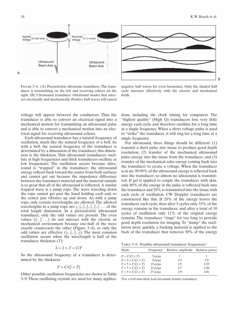
voltage will appear between the conductors. Thus thetransducer is able to convert an electrical signal into amechanical motion for transmitting an ultrasound pulseand is able to convert a mechanical motion into an elec-trical signal for receiving ultrasound echoes.

Each ultrasound transducer has a natural frequency ofoscillation, much like the natural frequency of a bell. Aswith a bell, the natural frequency of the transducer isdetermined by a dimension of the transducer; this dimen-sion is the thickness. Thin ultrasound transducers oscil-late at high frequencies and thick transducers oscillate atlow frequencies. The oscillation occurs because ultra-sound is “trapped” in the transducer; the ultrasoundenergy reflects back toward the center from both surfacesand cannot get out because the impedance differencebetween the transducer material and the material outsideis so great that all of the ultrasound is reflected. A similartrapped wave is a jump rope. The wave traveling downthe rope cannot get past the hand holding each end, sothe center just vibrates up and down. As with a jumprope, only certain wavelengths are allowed. The allowedwavelengths in a jump rope are 1–2 , 2–2 , 3–2 , 4–2 , 5–2 , 6–2 , 7–2 . . . of thetotal length dimension. In a piezoelectric ultrasoundtransducer, only the odd values are present. The evenvalues (2–2 , 4–2 . . .) do not interact with the electric ormechanical environment because one-half of the waveexactly counteracts the other (Figure 3–4), so only theodd values are effective (1–2 , 3–2 , 5–2 , 7–2 ). The most commonoscillation occurs when the wavelength is half of thetransducer thickness (T):

λ = 2 × T = C/F

So the ultrasound frequency of a transducer is deter-mined by the thickness.

F = C/(2 × T)

Other possible oscillation frequencies are shown in Table3–9. These oscillating crystals are used for many applica-

tions, including the clock timing for computers. The“highest quality” (High Q) transducers lose very littleenergy each cycle and therefore oscillate for a long timeat a single frequency. When a short voltage pulse is usedto “strike” the transducer, it will ring for a long time at asingle frequency.

For ultrasound, three things should be different: (1)transmit a short pulse into tissue to produce good depthresolution, (2) transfer of the mechanical ultrasoundpulse energy into the tissue from the transducer, and (3)transfer of the mechanical echo energy coming back intothe transducer to create a voltage. When the transduceris in air, 99.99% of the ultrasound energy is reflected backinto the transducer, so almost no ultrasound is transmit-ted. If gel is applied to couple the transducer with skin,only 80% of the energy in the pulse is reflected back intothe transducer and 20% is transmitted into the tissue witheach cycle of oscillation. CW Doppler transducers areconstructed like this. If 20% of the energy leaves thetransducer each cycle, then after 5 cycles only 33% of theenergy remains in the transducer, and after a total of 10cycles of oscillation only 11% of the original energyremains. The transducer “rings” for too long to providegood depth resolution for imaging. To “damp” the oscil-lation more quickly, a backing material is applied to theback of the transducer that removes 50% of the energy

UltrasoundBeam Axis

A

UltrasoundBeam Axis

ReceivedVoltage

AppliedVoltage 0.1–1 mVolt10–100 Volts

B

Figure 3–4. (A) Piezoelectric ultrasonic transducer. The trans-ducer is transmitting on the left and receiving echoes on theright. (B) Ultrasound transducer vibrational modes that inter-act electrically and mechanically. Positive half waves will cancel

Table 3–9. Possible ultrasound transducer frequencies.a

Mode Frequency Relative amplitude Relative power

F = C/(2 × T) 3cy/µs 1 1F = 3 × C/(2 × T) 9cy/µs 1/3 1/9F = 5 × C/(2 × T) 15cy/µs 1/5 1/25F = 7 × C/(2 × T) 21cy/µs 1/7 1/49F = 9 × C/(2 × T) 27cy/µs 1/9 1/81

aFor a 0.63-mm-thick lead zirconium titanite transducer.

negative half waves for even harmonics. Only the shaded halfcycle interacts effectively with the electric and mechanicalfields.


each cycle. With 20% leaving through the front and 50%leaving through the back, only 30% remains after 1 cycle,9% after 2 cycles, and less than 1% after 4 cycles. This iscalled a low Q transducer because it wastes so muchenergy, but makes images with good depth resolutionbecause the transmitting pulse is so short and the receiv-ing response is so quick. The wasted energy makes thetransducer warm. Such transducers are also inefficientfrom an energy point of view.

Two new methods are used in modern transducers tolower the Q and improve depth resolution (Figure 3–5).One method is to couple the transducer more effectivelyto the skin by using a piezoelectric material with lowerimpedance or using a matching layer of intermediateimpedance, one-quarter wavelength thick, between thetransducer and the skin. The other method is to combinethe damping material with the piezoelectric material inthe transducer; piezoelectric columns span from elec-trode to electrode with damping material between thecolumns. The first method makes the transducer moreefficient as a transmitter and as a receiver. The secondmethod makes transmitting and receiving less efficient.

Broad Band and Narrow Band

Well-damped and well-coupled transducers create shortpulses that provide good depth resolution. When testedfor the presence of a series of frequencies, positive testsare found over a broad band of frequencies (Figure 3–6).

Lateral Direction in the Image UltrasoundBeam Pattern Width

Ultrasound pulses are sent into tissue along a beampattern that is established by the location, orientation,widths, and shape of the active ultrasound transducer.The beam pattern is quite complex. It is useful to begin with a simplified view of the ultrasound beam

Figure 3–5. Advanced transducer damping methods. The leftimage is a composite transducer and the right image is a backedtransducer with matching layer. Black is piezoelectric material.Wires are hooked to electrodes. The damping material betweenthe transducer columns on the left transducer and on the backof the right transducer is shown as clear. Electrodes are darkgray. Light gray is the quarter wavelength matching layer on thebottom face of the right transducer where it comes in contactwith the patient.A similar matching layer could be added to theface of the left composite transducer.

A B

C

Figure 3–6. (A) Broad bandwidth pulse. A short pulse has abroad bandwidth because so many frequencies exhibit anequally poor fit with the pulse. The results of each frequencytest are shown as a bar graph spectrum on the left. (B) Mod-erate bandwidth pulse. A long pulse has a moderate bandwidthbecause several frequencies exhibit a fit with the pulse. Note:the middle frequency is the best fit. The results of each fre-quency test are shown as a bar graph spectrum on the left. (C)Narrow bandwidth wave. The continuous wave has a narrowbandwidth because only one frequency exhibits a fit with thewave. The results of each frequency test are shown as a bargraph spectrum on the left.


pattern and then to include aspects of the complexity in steps.

In the simplest view, the ultrasound beam pattern is astraight line that extends into tissue along the axis of theultrasound transducer. If the ultrasound transducer is adisk, the beam pattern is a line through the center of thedisk perpendicular to the surface. In a slightly morecomplex view (Figure 3–7), the ultrasound beam patternis a cylinder extending from the face of the transducer.Because ultrasound is a wave, the shape of the ultrasoundbeam pattern includes diffraction effects that alter theshape of the beam pattern near the transducer (Fresnelzone), far from the transducer (Fraunhoffer zone), and atthe boundary between these regions (Transition zone). In

the Fresnel zone, there is a patchwork of regions of highintensity and low intensity. From the Transition zone intothe Fraunhoffer zone, the ultrasound beam pattern issmoother. The distance from the transducer face to theTransition zone (L) is determined by half the transducerwidth (W/2) and the wavelength (λ). In a circular trans-ducer (W/2) is the radius.

L = (W/2)/λ

Thus, with shorter wavelength or a larger diameter trans-ducer [that is if (W/λ) is larger], the length of the regionover which the beam converges increases. The width ofthe ultrasound beam at the transition zone is half of thetransducer width. By increasing the bandwidth of thetransducer, unwanted variations in the beam pattern aresmoothed out (Figure 3–8).

Focusing and Lateral Resolution

The width of the ultrasound beam pattern may bedecreased to improve lateral resolution by focusing. Toachieve focusing, a transducer may have a concave face,a lens added to the front, and/or segmentation into anarray with delayed action at the center. The beam diam-eter at the focus is narrow compared to the half trans-ducer width natural focus at the Transition zone (Figure3–9). Focusing causes the beam to be narrow at onedepth. With such a narrow beam, the space betweenclosely positioned reflectors can be identified as the beampasses between them. It is easy to obtain reflections fromobjects in tissue, but it is difficult to detect and display thespace between objects. The minimum separation distancebetween objects recognized as separate is the resolution.A smaller number is better. The lateral resolution is

Figure 3–7. Concepts of ultrasound beam patterns. Increas-ingly sophisticated concepts of ultrasound beam patterns. Fromleft to right: thin beam pattern, collimated beam pattern, beampattern with Fraunhoffer zone, beam pattern with Transitionzone natural focus and Fraunhoffer zone, beam pattern withFresnel zone, Transition zone natural focus, Fraunhoffer zone,and first-order sidelobes.

Figure 3–8. Beam pattern for damped transducers. The narrowband continuous wave transducer on the left has a complexFresnel zone and narrow sidelobes. The broad band, high pulserepetition frequency (PRF) transducer in the center and thebroad band, low PRF transducer on the right have a smoothedFresnel zone and broadened sidelobes due to the differences inpatterns for each of the frequency components.

Figure 3–9. Focusing of ultrasound beam patterns. Left: trans-ducer with concave face. Middle: transducer with lens. Right:phased focus transducer.


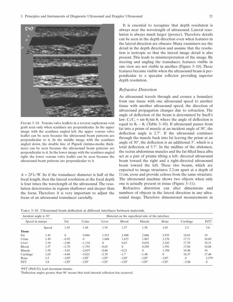
It is essential to recognize that depth resolution isalways near the wavelength of ultrasound. Lateral reso-lution is always much larger (poorer). Therefore detailscan be seen in the depth direction even when features inthe lateral direction are obscure. Many examiners see thedetail in the depth direction and assume that the resolu-tion is isotropic so that the lateral image detail is alsopresent. This leads to misinterpretation of the image. Bysteering and angling the transducer, features visible inone view are not visible in another (Figure 3–10). Thesefeatures become visible when the ultrasound beam is per-pendicular to a specular reflector providing superiordepth resolution.

Refractive Distortion

As ultrasound travels through and crosses a boundaryfrom one tissue with one ultrasound speed to anothertissue with another ultrasound speed, the direction ofultrasound propagation changes due to refraction. Theangle of deflection of the beam is determined by Snell’slaw: C2/C1 = sin θ2/sin θ1 where the angle of deflection isequal to θ2 − θ1 (Table 3–10). If ultrasound passes fromfat into a prism of muscle at an incident angle of 30°, thedeflection angle is 2.7°. If the ultrasound continuesthrough the muscle back into fat leaving the prism at anangle of 30°, the deflection is an additional 3°, which is atotal deflection of 5.7°. In the midline of the abdomen,the rectus abdominus muscles and the fat-filled linea albaact as a pair of prisms tilting a left- directed ultrasoundbeam toward the right and a right-directed ultrasoundbeam toward the left. These two beams, which areexpected to image structures 2.2cm apart at a depth of11cm, cross and provide echoes from the same structure.The ultrasound machine shows two objects when onlyone is actually present in tissue (Figure 3–11).

Refractive distortion can alter dimensions andnumbers of objects in the lateral direction in any ultra-sound image. Therefore dimensional measurements in

Figure 3–10. Venous valve leaflets in a reverse saphenous veingraft seen only when scanlines are perpendicular. In the upperimage with the scanlines angled left, the upper venous valveleaflet can be seen because the ultrasound beam patterns areperpendicular to it. In the middle image with the scanlinesangled down, the double line of Pignoli (intima-media thick-ness) can be seen because the ultrasound beam patterns areperpendicular to it. In the lower image with the scanlines angledright, the lower venous valve leaflet can be seen because theultrasound beam patterns are perpendicular to it.

Table 3–10. Ultrasound beam deflection at different interfaces between materials.

Incident angle is 30° Material on the superficial side of the interface

Speed in mm/µs Fat Urine Liver Blood Muscle Bone Cartilage PZTa

Speed 1.45 1.49 1.54 1.57 1.58 1.65 3.5 3.8TissueFat 1.45 0 0.884 1.915 2.498 2.686 3.935 18.05 19Urine 1.49 −0.92 0 1.068 1.672 1.867 3.159 17.71 18.69Liver 1.54 −2.08 −1.116 0 0.63 0.834 2.182 17.29 18.31Blood 1.57 −2.78 −1.793 −0.65 0 0.209 1.591 17.04 18.08Muscle 1.58 −3.01 −2.019 −0.86 −0.21 0 1.394 16.96 18Cartilage 1.65 −4.68 −3.621 −2.39 −1.7 −1.48 0 16.37 17.46Bone 3.5 −120b −120b −120b −120b −120b −120b 0 2.579PZT 3.8 −120b −120b −120b −120b −120b −120b −2.88 0

aPZT (PbZrTi), lead zirconium titanite.bDeflection angles greater than 90° means that total internal reflection has occurred.

A = 2Fλ /W. So if the transducer diameter is half of thefocal length, then the lateral resolution at the focal depthis four times the wavelength of the ultrasound. The reso-lution deteriorates in regions shallower and deeper thanthe focus. Therefore it is very important to adjust thefocus of an ultrasound transducer carefully.


the lateral direction are hampered by two factors: (1)poor lateral resolution and (2) lateral refractive distor-tion. This distortion becomes obvious only when dupli-cated structures are seen. A duplicated aorta is anunbelievable finding.A twin blastocyst in early pregnancyis believable. A duplicated aortic valve due to refractionin the peristernal cartilage is unbelievable.

Reflective duplications also occur such as the duplica-tion of the subclavian artery image due to reflection ofultrasound from the pleura. Refractive duplications showboth structures at generally the same depth; reflectiveduplications usually show the duplicate at a deeperdepth. Duplications appear in B-mode images and incolor Doppler images. Spectral waveforms can beobtained from both images. Therefore the only defenseagainst misdiagnosis is knowledge of anatomy and ofanatomic anomalies.

Sidelobes

Undesired sidelobes are also present in the beam pat-terns of ultrasound transducers, in addition to the desiredcentral beam patterns. Sidelobes degrade the image. Thesidelobes are shown in Figure 3–7 as lines angled out tothe left and right of the image. If the transducer is circu-lar, the beam pattern is symmetrical around the axis ofthe beam pattern. Thus, the sidelobe(s) look like a coneextending from the face of the transducer. The angle atwhich the sidelobes diverge (µ) can be computed fromthe ultrasound wavelength and the transducer width (W).

Sin α = [(2n + 1) × λ]/(2 × W)

n is any integer that is equal to 1 or greater. If (W/λ) islarge, then n can have many values and therefore manysidelobes form. The position of each sidelobe is deter-mined by the wavelength.

Sidelobes are a problem in imaging because strongreflectors in tissue that are located within a sidelobe at adistance of 3cm from the transducer will send a weakecho back to the ultrasound transducer that is indistin-guishable from an echo from a weak reflector in thestrong central beam at the same depth. The ultrasoundinstrument will show the sidelobe echo in the image as areflector along the central beam direction. This is one ofthe causes of poor ultrasound images.

The amplitude of the signal along the sidelobe portionof the beam is about 1/n of the central amplitude, dimin-ished further by the divergence of the sidelobe pattern.For n = 3, the sidelobe amplitude is 1/3, the power is 1/9,and the receiver sensitivity is 1/9. The overall pulse-echostrength is diminished 1/81 compared to a similar reflec-tor in the central lobe of the beam pattern. The reductionis greater when the effect of divergence is included. Sothe echo from the sidelobe is suppressed by about 20dB(about 1/100) compared to echoes from the beam axis.The difference in echogenicity between blood and muscleat 5MHz is about 30dB, so a strong reflector in the side-lobe could appear to be along the beam in the imageinside a blood vessel where the central lobe echoes areweak.

Other factors and methods can suppress sidelobes. Onemethod is to cut notches in the boundary of the trans-ducer so that the width W is fuzzy. This will smear thesidelobes. A similar method is to reduce the transmitstrength and receive sensitivity near the edge of the trans-ducer. This method is called apodization. The sidelobeposition depends on wavelength (λ) as well as width (W).Therefore, a broad band transducer with a range of wave-lengths will have smeared sidelobes with diminished sensitivity.

Sidelobe effects are more severe in Doppler kinds ofimaging because large differences in amplitude areignored in the signal analysis process, minimizing the dif-ference between sidelobe echoes and beam axis echoes.

Thickness Direction in the Image UltrasoundBeam Pattern Thickness

Most ultrasound instruments use one-dimensional elec-tronic array transducers to sweep the ultrasound beamacross a plane in tissue to form an image (Figure 3–12).The fixed focusing in the thickness direction causes thebeam pattern to be thick at most depths. Thereforeobjects in tissue that are outside the tissue “plane” areincluded in the image (Figure 3–13).

An additional interesting feature of Figure 3–13 is thepresence of reflected images. A moderately bright circu-

Figure 3–11. Duplication of abdominal aorta image due toultrasound beam refraction. Beginning at a depth of 11cm atthe center of the image, the 1.8-cm-diameter aorta can be seen(pulsating in real time); 2.2cm to the left of that image is asecond image of the aorta (pulsating in real time). A further 2.4cm to the left is the 2.1-cm-diameter inferior vena cava. The“duplication” of the aorta is due to ultrasound refraction fromthe linea alba/rectus abdominus muscles.2


surface and finally back to the transducer. The additionaltime for that “reverberant” trip forms the moderatelybright reflected image.A third deeper image is also barelydetectable.

Time of Image Acquisition FrameInterval/Sweep

When ultrasound image data are acquired, data alongeach line extending from the scanhead into tissue aregathered within one pulse-echo cycle. The conventionaltwo-dimensional image is formed by a series of such lines,each gathered in sequence. Common formats are sectorfrom a phase or curved array or raster from a linear array(Figure 3–14). With modern linear arrays, the location ofthe aperture can be selected as well as the direction ofbeam pointing (Figure 3–15).

The time to acquire data from each scan line is deter-mined by two factors: (1) the maximum depth from whichdata are coming, and (2) the number of pulse-echo cyclesrequired to acquire the data from the scanline (ensemblelength). The time for each pulse-echo cycle is T = 2 × D/Cwhere D is the maximum depth and C is the speed ofultrasound. For a maximum depth of 3cm, the timerequired is 40µs and for a maximum depth of 15cm, thetime required is 200µs. For B-mode imaging, the ensem-ble length is 1 and for typical Doppler color flow imaging,the ensemble length is 8 (Table 3–11).

In a typical Doppler color flow image that is 3cm wide(Figure 3–15), the images are formed from 128 B-modescanlines and 64 color scanlines. The B-mode scanlinesextend to a depth of 6cm (requiring 80µs) for each of the128 scanlines. The B-mode portion of the image requires(80µs × 128) 10.2ms for image formation.The color scan-lines extend to a depth of 3cm (requiring 40µs eachcycle) with an ensemble length of 8 requiring (40µs × 8)320µs for each of the 64 scanlines. The color Dopplerportion of the image requires (320µs × 64) 20.5ms forimage formation. The total time to create the image is(10.2ms + 20.5ms) 30.7ms, which nearly matches the 33ms time for each image in a standard ultrasound

Figure 3–12. Different arrangements of ultrasound transduc-ers from the patient view. Upper left: circular single elementtransducer. Upper center: annular array transducer for elec-tronic focusing. Upper right: linear array transducer for elec-tronic beam pointing in the lateral direction and fixedmechanical focus in the thickness direction. Lower left: singleelement “star” transducer to suppress sidelobes; a five-pointdesign or seven-point design is preferred because of fewer sym-metries. Lower center: two-dimensional array to steer the beamelectronically in two directions for three-dimensional imaging.Lower right: 1.5-dimensional array to steer the beam electron-ically in the lateral direction and electronically focus the beamin the thickness direction.

Figure 3–13. Five-millimeter-diameter straw in cross sectionand longitudinal section. To demonstrate the effect of ultra-sound image thickness on the image of a 5-mm-diameter veingraft, a 5-mm-diameter drinking straw is imaged in a water tank.A wire was attached to the side, outside the lumen. In crosssection (left) the wire can be seen outside the lumen. In longi-tudinal section on the right, the wire image appears to be withinthe lumen between the superficial and deep walls. The strongspecular (mirror like) reflections from the superficial and deepwalls combined with excessive image gain cause a “blooming”of the image that smears the echoes making the superficial anddeep walls appear thicker than they are. Reducing the ultra-sound transmit power will provide a proper image of the per-pendicular wall thickness.

Figure 3–14. Image scan formats. Left: sector format from aphase array. Middle: sector format from a curved linear array.Right: raster format from a straight linear array.

lar image of the straw appears below the “real” image.This deeper image is formed because of ultrasound thatreflects from the lower straw surface, back up to theupper straw surface, then back down to the lower straw


(National Television Standard Code) at 30 images persecond. If greater depths are required, then more time isrequired for each scanline and either the number of scan-lines or the frame rate must be sacrificed.

In “real time” imaging, a frame is not formed instantly,but the data are acquired systematically from left to right. In Doppler color flow imaging, the data for colorlines are acquired in sequence across the 3cm imagewidth in 0.02s (20ms); the acquisition proceeds from left to right at a speed of 150cm/s. This speed should

be compared with the speeds in the vascular system:wall motion <1cm/s, average arterial blood velocity = 30cm/s, and pulse propagation speed = 1000cm/s. It takesabout five cardiac cycles for blood to travel 150cm fromthe heart to the toes; it takes only 0.15s for the pulse to travel from the heart to the toes. Note that the speedof the Doppler acquisition line moves across the imagemore slowly than the pulse propagation speed. Thiscauses a time distortion in all color flow images (Figure3–16).

ACTIVE

A

APERTURE

B

Figure 3–15. (A) Modern phased-linear array beam steering.The ability to steer the beam pattern to a variety of angles forB-mode imaging is easier that to steer to a variety of angles forDoppler data. (B) Receiver channel echoes from each trans-ducer. The echoes received by each of 32 transducer elements

are displayed. Before adding the transducer data together,“beam forming” time delays are introduced on each channel toalign the echoes from a particular depth and location, then thedata from the channels are added to produce “beam formed”RF data for demodulation and display.


Table 3–11. Ultrasound modes and factors.a

Ultrasound operating modes

Color power Color flow Pulsed DopplerFactor B-mode angiography imaging waveform CW Doppler Harmonic imaging

Ultrasound frequency b c c c c Depressed Tx Elevated RcvUltrasound bandwidth Wide Moderate Moderate Moderate Narrow Broad splitDemodulation method Amplitude Phase Phase Phase Phase Band filtered/pulse invertEnsemble length 1 8 8 128 NA 1 or 2PRF Max Low Max Max 0 Max or max/2Filter method None Hi pass Hi pass Hi pass Hi pass Dual bandAnalysis method Square sum Variance Lambda FFT Heterodyne Square sumDisplay method Gray Colorize Bicolor Gray/V-t Audio GrayFrame rate High Low Moderate 0 0 High or moderateAveraging None Time and space Time None Time or none None or difference

aCW, continuous wave; PRF, pulse repetition frequency; FFT, fast Fourier transform.bThe dynamic range of echogenicity of solid tissues in ultrasound images is about 42dB (7 bits in a computer) and most instruments are capableof processing a dynamic range of 96dB (16 bits). Thus, echoes attenuated by 54dB still have the full dynamic range. A soft tissue layer that atten-uates ultrasound by 10dB is 67 wavelengths (from the attenuation discussion). So the roundtrip path of (67 × 54/10) 360 wavelengths defines themaximum imaging depth, or 180 wavelengths deep.cThe echogenicity of blood is 54dB (9 bits) lower than the brightest solid tissues in ultrasound images. Thus, for attenuation and Doppler fromblood in the presence of solid tissues, 42dB (7 bits) remains. Blood echogenicity increases with the fourth power of the frequency of ultrasound.Selection of the best ultrasound frequency depends on the balance between increased blood echogenicity and increased attenuation. For bloodvessels in liver (0.5dB/MHz/cm) the best ultrasound frequency is F = 1.7cmMHz/d where d is the depth of the blood vessel in cm.

Figure 3–16. The effect of image sweep speed on color flowimages.These are three images of the same segment of an arterytaken in sequence. Although we intend to show distance dis-played along the horizontal dimension, because of the slowsweep speed compared to the pulse propagation speed, the hor-

izontal dimension shows time. Peak systole shows as an aliasedblue velocity. In the bottom image, the Doppler data wereacquired near the left edge of the image during peak systole; inthe middle image, the Doppler data were acquired near theright edge of the image during peak systole.


The interaction between the pulse propagation speedand the Doppler acquisition speed suggests that a “sys-tolic velocity bolus” is just 2cm long, however, high systolic velocities appear at the toes while they are stillpresent at the aortic valve during systole.

Learning about the Tissues within Voxels

In modern ultrasound systems, the information displayedin each pixel about the corresponding voxel depends onthe selection of 10 factors: (1) the frequency of the ultra-sound pulse transmitted into tissue—“ultrasound fre-quency,” (2) the shape and duration of the ultrasoundpulse transmitted into tissue—“ultrasound bandwidth,”(3) the measurements made on the echo that come fromthe voxel—“demodulation method,” (4) the number of times that similar pulse-echo cycles are from thevoxel—“ensemble length,” (5) the time interval betweenthe pulse-echo cycles—“pulse repetition interval” (the

inverse of the pulse repetition frequency, PRF), (6) the filter method, (7) the analysis method, (8) the displaymethod, (9) the time required to update the other pixelson the screen—“frame interval” (the inverse of framerate), and (10) averaging between times and/or betweenpixels. The basic modes of ultrasound imaging can becharacterized by the alternative choices between the pos-sibilities of each of these factors.

The process of voxel interrogation has two parts: ananalog part and a digital part. In modern ultrasound scan-ners, most of the processing is done digitally. In old instru-ments everything was done with analog electronics.Figure 3–17 diagrams the analog signal portion of amodern instrument. This Figure is the basis for describ-ing the methods.

The ultrasound transmit pulse consists of a selectednumber of cycles. Transmit voltages applied to the trans-ducer range from 4 to 400V. The echo is segmented intopixels that are equal in length to the transmit pulse. Inmodern ultrasound imaging systems, the radio frequencyoscillations in each pixel are converted to a digital signal.The voltages along the oscillation are measured, fourtimes for each cycle, and the measured numbers are com-bined to form the digital signal. This process is called dig-itization. In modern instruments, each measurement hasa dynamic range of 16 bits (binary digits). Each operat-ing mode has a different pulse protocol and computationmethod.

Each of the following modes will be described usingthe same format. The number of cycles in the transmitpulse will be specified; this number will be called m. Theduration of each received pixel is equal to the transmitpulse duration.The oscillations in each received pixel willbe digitized at a frequency equal to four times the trans-mitted frequency, so there will be 4m sampled measure-ments digitized. Each of those sampled voltages will beidentified by number. In the case in Figure 3–17 with twocycles transmitted, there are two cycles in each receivedpixel and 4 × 2 or 8 samples in each pixel. The sampledvoltages are called V1, V2, V3, V4, V5, V6, V7, and V8. Finally,we may need to transmit along the ultrasound beam linemore than once to determine if the tissue is moving. Thenumber of times that we transmit, called ensemble length,will be called k. From here, the method is as simple as anincome tax form.

B-Mode Imaging at 5MHz

The length of the transmit pulse is short to create the bestdepth resolution, therefore m = 1. At 5MHz, one cyclelasts just 0.2µs. The echo digitizing rate is four times thetransmit frequency or 20MHz. The pixel is short, con-taining just one cycle, so we digitize just four voltages,called V1, V2, V3, and V4. Now we calculate the energy inthat 0.2-µs segment of the echo.

1

1 3

2 4 6 8 2 4 6 8 2 4 6 8 2 4 6 8

5 7 1 3 5 7 1 3 5 7 1 3 5 7

2 3 4

Figure 3–17. Ultrasound echo signals and demodulation.Upper: ultrasound transmit pulse. Middle: radio frequencyultrasound echo segmented into pixels. Lower: pixels parsed fordigitization.


Echo energy for each pixel = V 12 + V 2

2 + V 32 + V 4

2

The pixels with the highest energies are displayed aswhite on the screen and the pixels with the lowest ener-gies are displayed as black. An inverted gray scale or col-orized scale may also be used.

Before display, time gain compensation is applied. Fora pixel representing depth d from a tissue with attenua-tion rate A in dB/cm/MHz and ultrasound frequency F,the measured pixel voltage (square root of energy) ismultiplied by 1.26AxdxF.

The eye can see only 16 levels of gray. Video screensdisplay about the same. To convert 256 possible bright-ness levels into 16 levels of gray, the brightness levels areusually converted by postprocessing into a logarithmicbrightness scale using Table 3–12.

Digitizing for Flow Measurement

To prepare for the flow imaging methods, we should showhow to determine the amplitude and phase of the echooscillation in the pixel. It is equal to the square root of the energy. The computation requires two numbers, Iand Q.

I = V1 − V3

and

Q = V2 − V4

With algebra you can show that

Energy = I2 + Q2

if

V1 × V3 + V2 × V4 = 0

which is true in the absence of harmonics that result fromhigh ultrasound intensities or the presence of ultrasoundcontrast agents.

I and Q can be used to form a diagram (Figure 3–18) that shows both the phase and the amplitude of the wave. The amplitude is shown as distance from the origin of the plot and the phase is shown as angle.This phase map forms the basis of the flow imagingmethods.

Table 3–12. Conversion of time gain compensation adjusted received voltages into abrightness scale.a

0 1 2 3 5 7 11 15 22 31 45 63 90 127 181 2550 1 2 3 4 6 8 12 16 23 32 46 64 91 128 1820 1 2 3 4 5 6 7 8 9 10 11 12 13 14 15

aUpper row: upper bound of voltage range. Middle row: lower bound of voltage range. Lower row:corresponding brightness level.

+3I Q I R I Q I Q

1 2 3 4 5 6 7 8

1 2 3 4 5 6 7 8

I Q I Q I Q I Q

1 2 3 4 5 6 7 8

I Q I Q I Q I Q

+3

I

2

1

7

6

9

θ

9

0,8

3

4

5 A = 12

Q

–3

–3

0

1

2

3

4

5A

+

θ

+3

–3

7

8

6

I = V1 – V3 + V5 – V7I = 0 – 0 + 0 – 0 = 0

Q = V2 – V4 + V6 – V8Q = 3 – (–3) + 3 – (–3) = 12

I = 2 – (–2) + 2 – (–2) = 8

Q = 2 – (–2) + 2 – (–2) = 8

I = (–3) – 3 + (–3) – 3 + (–3) = –12

Q = 0 – 0 + 0 – 0 = 0

Figure 3–18. Formation of a phase diagram from an ultrasoundecho pixel.

Autocorrelation Doppler

For all Doppler methods, the length of the transmit pulseis long, about 5 cycles or 1µs at 5MHz to ensure that thephase measurement is accurate. The echo digitizing rate


is 20MHz. The pixel is long containing five cycles, so 20voltage values are digitized to represent the voxel, V1 toV20. Then the phase of the echo in the voxel is calculatedby computing the components I and Q.

I = V1 − V3 + V5 − V7 + V9 − V11 + V13 − V15 + V17 − V19

and

Q = V2 − V4 + V6 − V8 + V10 − V12 + V14 − V16 + V18 − V20

The measurement produces a single value on the I vs. Qphase plane (Figure 3–19). From the value, the amplitudecan be determined, but the phase has little meaning.The amplitude is the distance from the origin to the measurement. The energy is the square of the amplitude.By the Pythagorean theorem, the echo energy is I2 + Q2.

If the process of transmitting a pulse along a beampattern and receiving an echo from the selected depth isrepeated eight times, the resulting echo samples from thevoxel under investigation can be compared. If the tissuein the voxel has neither moved nor changed, then overthe period of the sampling, all samples are identical. If,however, all the tissue in the sample volume is movingtoward the ultrasound transducer, then the magnitudewill stay constant, but the phase of the echo will progressively change and each of the echoes will contribute a point to a circle of rotation around the origin (Figure 3–20). The number of samples collectedfrom each voxel, to form this circle, is called the ensem-ble length.

In Figure 3–20, in each pulse repetition interval (PRI =1/PRF), the phase of the echo has moved 1/8 cycle toward the transducer. The velocity component toward

the transducer is

VD = dp × λ/(2 × PRI) = dp × λ × PRF/2= (dp/PRI) × (C/F) × (1/2)

where = dp is the fraction of a complete cycle that thephase has shifted between one echo to another, λ is theultrasound wavelength (C/F), 2 accounts for the roundtrip of the ultrasound, PRI is the time between echosamples, and PRF is the number of echo samples persecond.

The component of the blood velocity measured by theDoppler is the leg of a right triangle. A right triangle canbe circumscribed with a semicircle with the hypotenuse(the real velocity vector) shown in Figure 3–21. The com-

I

Q

Figure 3–19. I/Q plot for one pulse-echo cycle.

I

3 2

1

8

76

5

4

3

Q

Figure 3–20. I/Q plot for eight pulse-echo cycles from tissuemoving through the sample volume.

Vbloodθ

VDoppler

Figure 3–21. Component of blood velocity measured byDoppler.


ponent velocity is represented by a cord of the circleformed by the blood velocity as diameter.

VD × cos θ = VD = (dp/PRI) × (C/F) × (1/2)= (f/2) × (C/F)

This is the well-known Doppler equation where (dp/PRI) is known as the Doppler frequency and happens,by fortunate chance, to be in the audible frequency range.

Unfortunately, in many cases, the interrogated Voxelcontains echogenic solid tissue as well as moving bloodso the phase diagram usually looks like Figure 3–22. Thephase circle is rotating in a counterclockwise direction sothe velocity component is away from the transducer. Thestationary echo S makes analysis more difficult. If only

two pulse-echo cycles were taken, then an incorrectvelocity measurement would result. Although the direc-tion of rotation appears to be counterclockwise, as indi-cated by the arrow suggesting flow away from thetransducer in Figure 3–23, the flow could be aliased, twiceas fast toward the transducer.

In a color flow image, flow toward the transducer indi-cated by clockwise rotation on the I/Q diagram is usuallyshown as a red pixel on the image and flow away fromthe transducer indicated by counterclockwise rotation onthe I/Q diagram is usually shown as a blue pixel on theimage. If the points do not form a uniform circle on theI/Q phase diagram, then the signal contains variance;cardiac color Doppler systems show high variance as agreen pixel on the image.

Color Power Angiography

Blood vessels usually are parallel to the skin and Dopplerultrasound beams are nearly perpendicular to the skinand vessels. Therefore, the Doppler examination angle isusually greater than 45° to the vessel axis. For conven-ience and consistency, many examiners use a Dopplerexamination angle of 60° between the ultrasound beampattern and the vessel axis. However, the normal bloodflow in a blood vessel is helical, converging into stenosesand diverging downstream. Therefore, color Dopplerimages usually contain intriguing color changes that canbe confusing. To avoid the confusion of “too much infor-mation” some instruments provide a feature called “colorpower angiography,” which shows pixels with bloodmotion in color without showing direction.These systemsare based on an ensemble of pulse-echo cycles plotted ona phase diagram such as Figure 3–24.

I

Q7 6

5

4

32

1

8

S

Figure 3–22. I/Q phase diagram with stationary echo S.

36

14 7

2

58

I

Q

Figure 3–23. I/Q phase diagram with stationary echo S andhigh velocity flow.

I

Q

1

27

468

53

Figure 3–24. I/Q diagram for color power angiography.


In the example, data from a voxel acquired by eightpulse-echo cycles are shown. All of the echoes fall withinthe shaded region. The area of the shaded region on theI/Q diagram is the “Doppler power.”

Fast Fourier Transform Spectral Waveform

The fast fourier transform (FFT) spectral waveform iscreated from the same kind of data as shown in Figures3–18 through 3–23.The FFT spectrum uses 128 pulse-echocycles for input data from a single voxel in tissue for eachspectrum. A waveform is a collection of 100 spectra persecond. Each I/Q phase diagram contains 128 points. Theperiod of data gathering is about 10ms (for a PRF of 12.8kHz). The voxel (sample volume) is about 1mm across. Ifthe blood velocity is 100cm/s (1000mm/s), a cluster of redblood cells will cross the voxel in 1ms; during the 10-msdata acquisition period, the blood in the voxel will becompletely exchanged 10 times. There is no relationshipbetween the phase of the echo of one cluster of red bloodcells and another. Therefore every millisecond (13 pulse-echo cycles) the point on the phase diagram is unrelatedto the prior phase. This introduces transit time spectralbroadening into the spectral waveform.3 Spectral broad-ening also occurs because of fluctuations in the bloodvelocity and because of system noise. The spectral broad-ening can be manipulated by adjusting the voxel size. Itcan also be used to measure “transverse velocity.” Spec-tral broadening and spectral shape, however, are mostuseful for figuring out complex flow dynamics becausethey show all of the velocities all of the time.

A spectral waveform from a voxel shows the detailedtime history of the flow through that voxel. Two-dimen-sional color flow imaging shows a single velocity for eachvoxel between 10 and 30 times per second (frame rate).Hemodynamic eddies can oscillate at frequencies of 50Hz or greater. The FFT waveform, displayed 100 timesper second, can show those eddies.

Conclusion

Over the past half century noninvasive examination ofvascular disease has advanced greatly as Dopplermethods were augmented with B-mode imaging to formduplex scanners. Duplex pulse Doppler spectral wave-form analysis has become the standard noninvasivemethod for evaluating arterial stenoses, venous obstruc-tion, and venous valve incompetence. The evolution hasbenefited from contributions by both manufacturers andclinical examiners. Confusions and disagreements are anatural part of that process. One of those disagreements

is over the visualization of lesions and plaques in ultra-sound B-mode images. Many examiners have classifiedplaque as “hard,” “soft,” “heterogeneous,” “homoge-neous,” or “intimal thickening.” In our experience,B-mode imaging of vascular structures has not providedclinically useful information. Another disagreement is the question of choice of Doppler examination angle. Because the geometry of arteries and veins prevents the use of coaxial ultrasound beams (which are possible when examining the aortic and mitralvalves), some examiners believe that the cosine of theexamination angle can be used to “correct” the velocitymeasurement taken at the poor angles permitted by anatomical restrictions. Other examiners believe that the definition of velocity is obscure, that a consistentexamination angle should be used, and that the resultant velocity value should be used only in compari-son with an empirical standard. We subscribe to the latter view.

All examiners hope that new examination methodssuch as color flow imaging can improve diagnostic accu-racy. This is an elusive goal because each examinationmethod has strengths and weaknesses. Comparisonbetween methods yields surprises and increased under-standing. A comparison between velocity measurementstaken with color flow imaging and taken with Dopplerspectral waveform (Figure 3–25) demonstrates the dis-agreement in results that invite resolution.

To ensure that the different modes of Doppler display work in concert, the methods of two-dimensionalcolor Doppler imaging, color Doppler M-mode imaging and spectral waveform imaging should be combined (Figure 3–26). This permits an exact compari-son between the Doppler FFT spectral waveform velocity information and the autocorrelation colordisplay. Note that the two methods of velocity determination occur in different sections of the ultra-sound system and use different ensemble lengths.Therefore, the velocity ranges and baseline shift can beset differently.

Ultrasound instruments are passing through a newrapid evolution, plunging in cost and size. It is now possible for a patient to buy an ultrasound system to wear and obtain constant examination.4 It is also possible to obtain a correct velocity measurement from peripheral blood vessels without assumptions about the examination angle5–8 and to measure tissue pulsations and vibrations as small as 0.05µm. The depthderivative of displacement is pulsatility. It is possible to measure pulsatility due to capillary filling and displaythis information in ultrasound images.9–11 This method has been used by Robert Pretlow to show that canceroustissues in breast have pulse amplitudes three times as high as normal tissues. It has also been used by


John Kucewicz to show maternal and fetal pulsations inthe placenta.

With access to internet information services, it is easyto keep track of the latest advancements in the medicalliterature12 and the most recent patents.13

Acknowledgments. This work was supported by theDefense Research Projects Administration (DARPA)and the Office of Naval Research (ONR) N00014-96-1-0630.

References

1. Comess KA, Beach KW, Hatsukami T, Strandness DE Jr,Daniel-W. Pseudocolor displays in B-mode imaging appliedto echocardiography and vascular imaging: An update.J Am Soc Echocardiogr 1992;5(1):13–32.

2. Vandeman FN, Meilstrup JW, Nealy PA. Acoustic prismcausing sonographic duplication artifact in the upperabdomen. Invest Radiol 1990;25:658–63.

3. McArdle A, Newhouse VL, Beach KW. Demonstration ofthree-dimensional vector flow estimation using bandwidthand two transducers on a flow phantom. Ultrasound MedBiol 1995;21(5):679–92.

4. http://www.dxu.com/pci5000_f.html.5. Papadofrangakis E, Engeler WE, Fakiris JA. Measurement

of true blood velocity by an ultrasound system. U.S. Patent4265126: Assignees: General Electric Company, Schenec-tady, NY; Issued: May 5, 1981; Filed: June 15, 1979.

6. Beach K, Overbeck J. Vector Doppler medical devices forblood velocity studies. U.S. Patent 5409010: Board ofRegents of the University of Washington, Seattle, WA;Issued: April 25, 1995; Filed: May 19, 1992.

7. Overbeck J, Beach KW, Strandness DE Jr. Vector Doppler:Accurate measurement of blood velocity in two dimen-sions. Ultrasound Med Biol 1992;18(1):19–31.

Figure 3–25. Comparison between Doppler color velocity andspectral waveform velocity,The peak systolic velocity accordingto the aliased color flow image is 38 + 30 or 68cm/s. The peaksystolic velocity according to the aliased spectral waveform is74 + 70 or 144cm/s. The difference in measured values could bea difference in angle adjustment and/or a difference in the pro-cessing of color flow data vs. spectral waveform data. In spite ofthe high velocity, which is localized in the middle of the colorflow image, no stenosis is present in this artery. Arterial systoleoccurred by chance as the color flow data for the center of theimage were being acquired.

Figure 3–26. Combined spectral waveform and color M-modeimaging.


8. Beach KW, Dunmire B, Overbeck JR, Waters D, Billeter M,Labs KH,Strandness DE Jr.Vector Doppler systems for arte-rial studies, Part I: Theory. J Vasc Invest 1996;2(4):155–65.

9. Beach KW, Phillips DJ, Kansky J. Ultrasonic plethysmo-graph. U.S. Patent 5289820: Assignees: The Board ofRegents of the University of Washington, Seattle, WA;Issued: March 1, 1994; Filed: November 24, 1992.

10. Beach KW, Phillips DJ, Kansky J. Ultrasonic plethysmo-graph. U.S. Patent 5183046: Assignees: Board of Regents of

the University of Washington, Seattle, WA; Issued: Febru-ary 2, 1993; Filed: November 15, 1991.

11. Beach KW, Phillips DJ, Kansky J. Ultrasonic plethysmograph. U.S. Patent 5088498: Assignees: The Board of Regents of the University of Washington,Seattle, WA; Issued: February 18, 1992; Filed: January 18,1991.

12. http://www.ncbi.nlm.nih.gov/entrez/.13. http://www.uspto.gov/.

Download - Principles and Instruments of Diagnostic Ultrasound

Top Related