ARTICLE IN PRESS
Neurocomputing 71 (2008) 3295– 3302
Contents lists available at ScienceDirect
Neurocomputing
0925-23
doi:10.1
� Corr
matics a
Tel.: +8
E-m
journal homepage: www.elsevier.com/locate/neucom
Multistage RBF neural network ensemble learningfor exchange rates forecasting
Lean Yu a,b,�, Kin Keung Lai b, Shouyang Wang a
a Institute of Systems Science, Academy of Mathematics and Systems Science, Chinese Academy of Sciences, Beijing 100190, Chinab Department of Management Sciences, City University of Hong Kong, Tat Chee Avenue, Kowloon, Hong Kong
a r t i c l e i n f o
Available online 21 June 2008
Keywords:
RBF neural networks
Ensemble learning
Conditional generalized variance
Exchange rates prediction
12/$ - see front matter & 2008 Elsevier B.V. A
016/j.neucom.2008.04.029
esponding author at: Institute of Systems S
nd Systems Science, Chinese Academy of Sci
6 10 62565817; fax: +86 10 62541823.
ail address: [email protected] (L. Yu).
a b s t r a c t
In this study, a multistage nonlinear radial basis function (RBF) neural network ensemble forecasting
model is proposed for foreign exchanger rates prediction. In the process of ensemble modeling, the first
stage produces a great number of single RBF neural network models. In the second stage, a conditional
generalized variance (CGV) minimization method is used to choose the appropriate ensemble members.
In the final stage, another RBF network is used for neural network ensemble for prediction purpose. For
testing purposes, we compare the new ensemble model’s performance with some existing neural
network ensemble approaches in terms of four exchange rates series. Experimental results reveal that
the predictions using the proposed approach are consistently better than those obtained using the other
methods presented in this study in terms of the same measurements.
& 2008 Elsevier B.V. All rights reserved.
1. Introduction
Combining the outputs of multiple neural networks into anaggregate output often gives improved accuracy over anyindividual neural network output [13,23]. Initially, the genericmotivation of neural network ensemble procedure is based uponan intuitive idea that by combining the outputs of severalindividual neural networks, one might improve on the perfor-mance of a single generic one [10]. But this idea has been provedto be true only when the ensemble models are simultaneouslyaccurate and diverse enough, which requires an adequate trade-off between the conflicting conditions. That is, performanceimprovement can result from training the individual neuralnetworks to be decorrelated with each other [14] with respectto their errors. For this, ensemble learning and modeling havebeen a common research stream in the last few decades[3,6,8,10–14,17,22,23]. Over this time, the research stream hasgained momentum with the advancement of computer technol-ogies, which have made many elaborate computation methodsavailable and practical [22].
Actually, neural networks provide a natural framework forensemble learning. This is so, because neural networks are a kindof unstable learning techniques, i.e., small changes in the trainingset and/or parameter selection can produce large changes in thepredicted output. Many experiments have shown that the
ll rights reserved.
cience, Academy of Mathe-
ences, Beijing 100190, China.
generalization of single neural network is not unique, that is,the neural network’s solutions are not stable. Even for somesimple problems, different structures of neural networks(e.g., different number of hidden layers, different number ofhidden nodes and different initial conditions) result in differentpatterns of network generalization. In addition, even the mostpowerful neural network model still cannot cope well whendealing with complex data sets containing some random errors orinsufficient training data. Thus, the performance for these datasets may not be as good as expected [6,11,12,22].
Instability of the single neural network has hampered thedevelopment of better neural network models. Why can the sametraining data applied to different neural network models or thesame neural models with different initialization lead to differentperformance? What are the major factors affecting this differ-ence? Through the analysis of error distributions, it has beenfound that the ways neural networks have of getting to the globalminima vary, and some networks just settle into local minimainstead of global minima. In any case, it is hard to justify whichneural network’s error reaches the global minima if the error rateis not zero. Since the number of neural models and their potentialinitialization is unlimited, the possible number of resultsgenerated for any training data set applied to those models istheoretical infinite. The best performance we typically get is onlythe best one selected from a limited number of neural networks,i.e., the single model with the best generalization to a testing set.One interesting point is that, in a prediction case, other less-accurate predictors may generate a more accurate forecast thanthe most-accurate predictor. Thus, it is clear that simply selectingthe best predictors according to their performance is not the
ARTICLE IN PRESS
X1
X2
Xk
W0
W1
W2
Wm
+Y
Cm
C1
C2
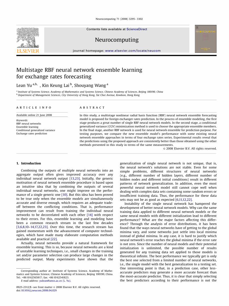
Fig. 1. The generic architecture of the RBF neural network.
L. Yu et al. / Neurocomputing 71 (2008) 3295–33023296
optimal choice. More and more researchers have realized thatmerely selecting the predictor that gives the best performance onthe testing set will lead to losses of potentially valuableinformation contained by other less successful predictors. Thelimitation of individual neural network suggested a differentapproach to solving these problems that considers those dis-carded neural networks, whose performance is less accurate aspotential candidates for new network models: a neural networkensemble model [8].
In addition, another important motivation behind ensemblelearning method integrating different neural network models isbased on the fundamental assumption that one cannot identifythe true process exactly, but different models may play acomplementary role in the approximation of this process. In thissense, an ensemble learning model is generally better than asingle model.
However, it is worth noting that there are still several mainproblems to be addressed. First of all, the existing neural networkensemble learning models are basically relied on the standardfeed-forward neural network models [3,6,8,10–14,17,22] such asback-propagation neural networks (BPNN). But one main draw-back of the standard feed-forward neural networks is that theirlearning processes are time-consuming and have a tendency toget stuck at local minima [7]. For this reason, this study adoptsanother neural network type—radial basis function (RBF) neuralnetwork for ensemble learning purpose. As [2,19] indicated, theRBF neural network can overcome the above drawbacks to obtaingood performance.
Second, the output of the existing neural network ensemblemodel is a weighted average of the outputs of each neuralnetwork, with the ensemble weights determined as a function ofthe relative error of each network determined in training [13,23]methods include simple averaging method [22,23], simple meansquared error (MSE) method [1,23], stacked regression method[4,23] and variance-based weighting method [10,23]. However,numerous empirical experiments have been demonstrated thateach existing method has its own drawbacks, as will be indicatedin the following section. For this problem, the study proposes anovel ensemble strategy—RBF-based ensembling method. That is,we use another RBF network for neural network ensemble. In thissense, the RBF network ensemble learning model is actually anembedded learning model or a modularized learning model.
Third, in the existing neural network ensemble learningmodels, most studies focused on the ensemble strategy and theensemble learning processes are often neglected. For this issue,this study proposes a multistage process to formulate an overallensemble learning procedure.
In terms of the above three aspects, this study will formulate amultistage RBF neural network ensemble learning model in anattempt to solve the three main issues mentioned above. Forfurther illustration and verification, this proposed RBF neuralnetwork ensemble learning model is applied to exchange ratesprediction. The main goal of the proposed RBF ensemble learningmethod is to overcome the shortcomings of the existing neuralnetwork ensemble methods and ameliorate forecasting perfor-mance. The main objectives of this study are three-fold: (1) toshow how to construct a multistage RBF neural network ensemblelearning model; (2) to show how to predict exchange rates usingthe proposed RBF neural network ensemble learning model and(3) to display how various methods compare in their performancein predicting foreign exchange rates. According to the threeobjectives, this study mainly describes the building process of theproposed nonlinear ensemble learning model and the applicationsof the RBF neural network ensemble learning approach in foreignexchange rate forecasting between the US dollar and four othermajor currencies: British pounds, euros, German marks and
Japanese yen, while comparing forecasting performance with allkinds of evaluation criteria.
The rest of this study is organized as follows. The next sectionbriefly describes the RBF neural network. Section 3 presents thebuilding process of the multistage RBF neural network ensemblelearning model in detail. For illustration purpose, the empiricalresults of the exchange rates of four main currencies are reportedin Section 4. The conclusions are contained in Section 5.
2. An overview of the RBF neural network
The RBF neural network [2,19] is generally composed of threelayers: input layer, hidden layer and output layer. The input layerfeeds the input data to each of the nodes of the hidden layer. Thehidden layer of nodes differs greatly from other neural networksin that each node represents a data cluster which is centered at aparticular point with a given radius. Each node in the hidden layercalculates the distance from the input vector to its own center. Thecalculated distance is transformed via some basis function and theresult is output from a node. The output from the node ismultiplied by a constant or weighting value and fed into theoutput layer. The output layer consists of only one node whichacts to sum the outputs of the previous layer and to yield a finaloutput value [23]. A generic architecture of an RBF network with k
input and m hidden nodes is illustrated in Fig. 1.The computation process of the RBF neural network follows
the following procedures. When the network receives a k
dimensional input vector X, the network computes a scalar valueusing the following formula
Y ¼ f ðXÞ ¼ w0 þXm
i¼1
wijðDiÞ (1)
where w0 is the bias, wi is the weight parameter, m is the numberof nodes in the hidden layers of the RBF neural network, and j(Di)is the RBF. In this study, the Gaussian function is used as RBF, asshown below
jðDiÞ ¼ expð�D2i =s
2Þ (2)
where s is the radius of the cluster represented by the centernode, the Di represents the distance between the input vector Xand all the data centers. It is clear that j(Di) will return valuesbetween 0 and 1. Usually, the Euclidean norm is used to calculatedistance, but other metrics can also be used. The Euclidean normis calculated by
Di ¼
ffiffiffiffiffiffiffiffiffiffiffiffiffiffiffiffiffiffiffiffiffiffiffiffiffiffiffiXk
j¼1
ðxj � cjiÞ2
vuut (3)
where c is a cluster center for any of the given nodes in the hiddenlayer.
ARTICLE IN PRESS
L. Yu et al. / Neurocomputing 71 (2008) 3295–3302 3297
Complex nonlinear systems such as foreign exchange ratesdata are generally difficult to model using linear regressionmethodologies [19]. Dissimilar to the regression, neural networksare nonlinear and their parameters are determined by somelearning techniques and search algorithms such as error backpropagation and steep gradient algorithm. The main shortcomingsof the standard BPNN are that their learning process is slow, andthus it is a time-consuming process. Furthermore, they have atendency to get stuck at local minima [7]. But RBF neuralnetworks overcome the above problems to obtain good perfor-mance since their parameters that need to be trained are the onesin the hidden layer of the network. Finding their values is thesolution of a linear problem and can be obtained throughinterpolation [2]. Therefore, their parameters are found muchfaster than in BPNN. Furthermore, the RBF neural network canusually reach near perfect accuracy on the training data setwithout trapping into local minima [19].
3. Building process of the RBF neural networkensemble model
In this section, a three-stage RBF neural network ensemblelearning model is proposed for exchange rates prediction. In thefirst stage, multiple single RBF neural network predictors areproduced in terms of diversification. In the second stage, anappropriate number of RBF neural network predictors are chosenfrom the considerable number of candidate predictors generatedby the previous stage. That is, the previous two stages adopt anunderlying ‘‘overproduce and choose’’ paradigm. In the final stage,the selected RBF neural network predictors are combined into anaggregated output in an embedded learning way in terms ofanother RBF neural network model.
3.1. Producing multiple single RBF neural network predictors
According to bias-variance trade-off principle [24], an ensem-ble model consisting of diverse models with much disagreementis more likely to have a good performance. Therefore, how togenerate the diverse model is a crucial factor. For RBF neuralnetwork model, several methods have been investigated for thegeneration of ensemble members making different errors. Suchmethods basically depended on varying the parameters ofRBF neural networks or utilizing different training sets. Inparticular, the main methods include the following four ways
(1)
Varying different RBF neural network architecture: by chan-ging the number of nodes in hidden layer, diverse RBF neuralnetworks with much disagreement can be created.(2)
Utilizing different cluster center of the RBF neural networks:through varying the cluster center c of the RBF neuralnetworks, different RBF neural networks can be produced.(3)
Adopting different cluster radius of the RBF neural networks:through varying the cluster center o of the RBF neuralnetworks, different RBF neural networks can be generated.(4)
Using different training data: by re-sampling and pre-processing data, we can obtain different training sets. Typicalmethods include bagging [5], cross-validation (CV) [10],stacking [20], and boosting [15]. With these different trainingdatasets, diverse RBF neural network models can be produced.In the above methods, we can use any one of the four ways. Ofcourse, diverse RBF neural network ensemble candidates could becreated using a hybridization of two or more of the abovemethods, e.g., different RBF network architectures plus different
training data [16]. In this study, we adopt a certain single way tocreate ensemble members. Once some individual RBF neuralnetwork predictors are created, we are required to select somerepresentative members for ensemble purposes to save computa-tional costs and speedup the computational process.
3.2. Choosing appropriate ensemble members
Using the diverse RBF neural network model generated by theprevious stage and training data, each individual RBF neuralpredictor has generated its own result when facing a new sample.However, if there are a great number of individual members (i.e.,the previous stage overproduces multiple ensemble members or apool of ensemble members), we need to select a subset ofrepresentatives in order to improve ensemble efficiency and savecomputational cost. As Yu et al. [22] claimed, not all circum-stances are satisfied with the rule of ‘‘the more, the better’’. Thus,it is necessary to use an appropriate method to choose ordetermine the number of individual neural network models(i.e., ensemble members) for ensemble forecasting purpose.Generally, we chose some ensemble members with error weakcorrelation for diverse RBF neural models. In the work of Yu et al.[22], they utilized a principal component analysis (PCA) techniqueto select the appropriate number of ensemble members andobtained good performance from experimental analysis. However,the PCA is a kind of data-reduction technique, which it does notconsider the internal correlations between different ensemblemembers. To overcome this problem, a conditional generalizedvariance (CGV) minimization method is proposed here.
Supposed that there are p neural predictors with n forecastvalues. Then the error matrix (e1,e2,y,ep) of p predictors isrepresented as
E ¼
e11 e12 � � � e1p
e21 e22 � � � e2p
..
. ... ..
.
en1 en2 � � � enp
2666664
3777775
n�p
(4)
From the matrix, the mean, variance and covariance of E can becalculated as
Mean : ei ¼1
n
Xn
k¼1
eki ði ¼ 1;2; . . . ; pÞ (5)
Variance : Vii ¼1
n
Xn
k¼1
ðeki � eiÞ2ði ¼ 1;2; . . . ; pÞ (6)
Covariance : Vij ¼1
n
Xn
k¼1
ðeki � eiÞðekj � ejÞ ði; j ¼ 1;2; . . . ;pÞ (7)
Considering Eqs. (6) and (7), we can obtain a variance–covariance matrix
Vp�p ¼ ðVijÞ (8)
Here, we use the determinant of V, i.e., |V| to represent thecorrelation among the p predictors. When p is equal to one,|V| ¼ |V11| ¼ the variance of e1 (the first predictor). When p islarger than one, |V| can be considered to be the generalization ofvariance: therefore, we call |V| as the generalized variance. Clearlywhen the p predictors are correlated, the generalized variance |V|is equal to zero. On the other hand, when the p predictors areindependent, the generalization variance |V| reaches its max-imum. Therefore, when the p predictors are neither independentnor correlated, the measurement of generalized variance |V|reflects the correlation among the p predictors.
ARTICLE IN PRESS
L. Yu et al. / Neurocomputing 71 (2008) 3295–33023298
Now we introduce the concept of CGV. The matrix V can bereformulated with the block matrix. The detailed process is asfollows: (e1,e2,y,ep) is divided into two parts: (e1,e2,y,ep1) and(ep1+1,ep1+2,y,ep), denoted as e(1) and e(2), i.e.,
E ¼
e1
e2
..
.
ep
2666664
3777775 ¼
eð1Þ
eð2Þ
!p1�1
p2�1
; p1 þ p2 ¼ p (9)
V ¼
V11
V21
V12
V22
!p1
p2
p1 p2
(10)
where V11, V22 represent the covariance matrix of e(1) and e(2).Given e(1), the CGV of e(2), V(e(2)|e(1)), can be expressed as
Vðeð2Þjeð1ÞÞ ¼ V22 � V21V�111 V12 (11)
The above equation shows the change of e(2) given that e(1) isknown. If e(2) has a small change under e(1), then the predictorse(2) can be deleted. This implies that the predictors e(1) can obtainall the information that the predictors e(2) reflect. Now we cangive an algorithm for minimizing the CGV below
(1)
Considering that the p predictors, the errors can be dividedinto two parts: (e1,e2,y,ep�1) is seen as e(1), (ep) is seen as e(2).(2)
The CGV V(e(2)|e(1)) can be calculated according to Eq. (11). Itshould be noted here that V(e(2)|e(1)) is a value, denoted as tp.(3)
Similarly, for the ith predictor (i ¼ 1,2,y,p), we can use (ei) ase(2), and other p�1 predictors are seen as e(1); then we cancalculate CGV of the ith predictor, ti, with Eq. (11).(4)
For a pre-specified threshold y, if ti oy, then the ith predictorshould be deleted from the p predictors. On the contrary, if ti4y, then the ith predictor should be retained.
(5) For the retained predictors, we can perform the previousprocedures (1)–(4) iteratively until satisfactory results areobtained.
3.3. Combining the selected members
Depended on the work done in previous stages, a collection ofappropriate ensemble members can be collected. The subsequenttask is to combine these selected members into an aggregatedpredictor in an appropriate ensemble strategy. For helping readerunderstand the following notations, the ensemble predictors canbe first defined. Suppose there are n individual RBF neuralnetworks trained on a data set D ¼ {xi, yi} (i ¼ 1,2,y,n). Aftertraining, n individual RBF neural network outputs, i.e.,f1(x),f2(x),y,fn(x) are generated. Through selection procedurepresented in Section 3.2, m RBF ensemble member,f1(x),f2(x),y,fm(x), are chosen. The current question of the RBFneural network ensemble forecasting is how to combine (en-semble) these selected members into an aggregate output y ¼ f(x),which is assumed to be a more accurate output. The general formof the model for such an ensemble predictor can be defined as
f ðxÞ ¼Xm
i¼1
wif iðxÞ (12)
where wi denotes the assigned weight of fi(x), and in general thesum of the weight is equal to one. In the RBF neural networkensemble forecasting, how to determine ensemble weights is akey issue. As earlier mentioned, there are a variety of methods for
determining ensemble weights in the past studies, which ispresented in the following. Generally, there are four ensemblestrategies, which are described below.
Typically, simple averaging [3,4,22,23] and weighted averaging[13,22] are the two main ensemble strategies. Of the weighted-averaging strategy, there are three variants: simple MSE approach[1,23], stacked regression method [4,23] and variance-basedweighting method [10,23].
Simple averaging method is one of the most frequently usedensemble approaches that are easy to understand and implement[3]. Some experiments [4,8] have shown that this approach byitself can lead to improved performance and it is an effectiveapproach to improve neural network performance. Specially, it ismore useful when the local minima of ensemble members aredifferent, i.e., when the local minima of ensemble networks aredifferent. Different local minima mean that ensemble membersare diverse. Thus, averaging them can reduce the ensemblevariance. Usually, the simple averaging method for ensembleforecasting is defined as
f ðxÞ ¼Xm
i¼1
wif iðxÞ ¼1
m
Xm
i¼1
f iðxÞ (13)
where the weight of each individual network output wopt,i ¼ 1/m.However, this approach treats each member equally, i.e., it
does not stress ensemble members that can make morecontribution to the final generalization. That is, it does not takeinto account the fact that some networks may be more accuratethan others. If the variances of ensemble networks are verydifferent, we do not expect to obtain a better result using simpleaveraging method [18]. In addition, since the weights in thecombination are so unstable, a simple average may not the bestchoice in practice [9].
The simple MSE approach estimates the linear weight para-meter wi in Eq. (12) by minimizing the MSE [1], that is, fori ¼ 1,2,y,m,
wopt;i ¼ arg minwi
Xk
ðwTi f iðxjÞ � djiðxjÞÞ
2
( )
¼Xk
j¼1
f iðxjÞfTi ðxjÞ
0@
1A�1Xk
j¼1
djiðxÞf iðxjÞ (14)
where d(x) is the expected value.The simple MSE solution seems to be reasonable, but, as
Breiman [4] has pointed out, this approach has two seriousproblems in practice
(1)
The data are used both in the training of each predictor, and inthe estimation of wi and(2)
Individual predictors are often strongly correlated since theytry to predict the same task.Due to these problems, this approach’s generalization abilitywill be poor. To address these two issues, another ensemblemethod called stacked regression is proposed.
The stacked regression method was proposed by Breiman [4] inorder to solve the problems associated with the previous simpleMSE method. Thus, the stacked regression method is also calledthe modified MSE method. This approach utilizes CV data tomodify the simple MSE solution, i.e.,
wopt;i ¼ arg minwi
Xk
j¼1
ðwTi giðxjÞ � djiðxjÞÞ
2
8<:
9=;; i ¼ 1;2; . . . ;m (15)
where giðxjÞ ¼ ðfð1Þ
i ðxj;DcvÞ; � � � ; fðkÞ
i ðxj;DcvÞÞT2 <K is a CV version
f iðxjÞ 2 <K and Dcv is the CV data.
ARTICLE IN PRESS
Output layer
Hidden layer
Radial basis function(Gaussian function)
Input layer
RBF1Output
RBF2Output
RBFmOutput
y
w1 w2
wm
� (x1, c)^ � (x2, c)^� (xm, c)^
xm^x1 x2
^
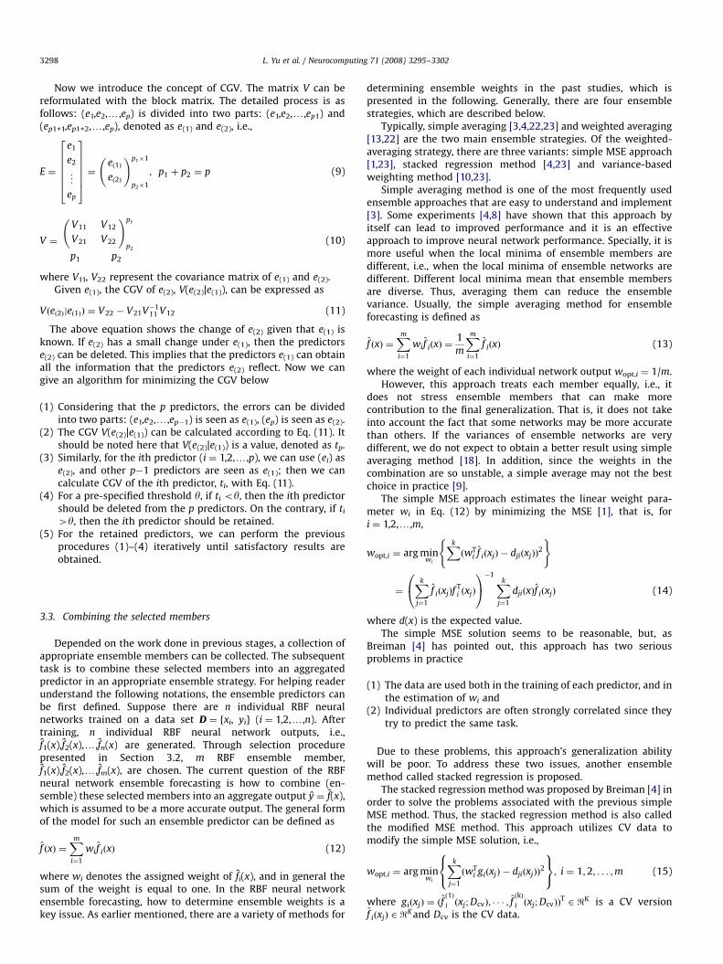
Fig. 2. The basic structure of RBF neural network ensemble forecasting model.
L. Yu et al. / Neurocomputing 71 (2008) 3295–3302 3299
Although this approach overcomes the limitations of thesimple MSE method, the solution is based on the assumptionthat the error distribution of each validated set is normal. Inpractice, however, this normal assumption does not always hold,and thus this approach does not lead to the optimal solution in theBayes sense [18].
Recently, another ensemble method based on the error-variance is proposed. Basically, the error-variance-based weight-ing ensemble approach is to estimate the weight parameter wi byminimizing error-variance si
2 [10]. That is, all ensemble predictorsare error-independent networks, and the optimal weights aredetermined by the following optimal problem, i.e.,
wopt;i ¼ arg minwi
Xmi¼1
ðwis2i Þ
2
( ); ði ¼ 1;2; . . . ;mÞ (16)
under the constraints Smi¼1wi ¼ 1and wiX0. Using the Lagrange
multiplier, the optimal weights are as
wopt;i ¼ðs2
i Þ�1Pn
j¼1ðs2j Þ�1; ði ¼ 1;2; . . . ;mÞ (17)
The variance-based weighting method is based on the assump-tion of error-independence. Moreover, as mentioned earlier,individual predictors are often strongly correlated for the sametask. This indicates that this approach has serious drawbacks forminimizing error-variance when neural predictors with strongcorrelation are included within the ensemble members.
According to the previous descriptions and literature review,the above four neural network ensemble strategies have widelybeen used, but we can also find that the weights of theseensemble methods are determined by the error or error variance.In practice, error-dependent network ensemble model may notoften obtain good forecasting performance when error is corre-lated each other [13]. Thus, the existing ensemble strategies interms of error or error-variance are insufficient. For this issue, thisstudy uses another RBF neural network as an ensemble tool toaggregate the ensemble members.
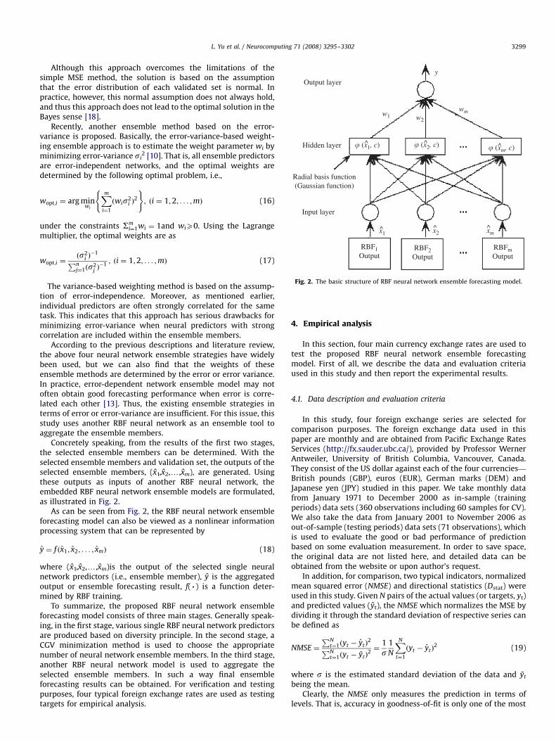
Concretely speaking, from the results of the first two stages,the selected ensemble members can be determined. With theselected ensemble members and validation set, the outputs of theselected ensemble members, (x1,x2,y,xm), are generated. Usingthese outputs as inputs of another RBF neural network, theembedded RBF neural network ensemble models are formulated,as illustrated in Fig. 2.
As can be seen from Fig. 2, the RBF neural network ensembleforecasting model can also be viewed as a nonlinear informationprocessing system that can be represented by
y ¼ f ðx1; x2; . . . ; xmÞ (18)
where (x1,x2,y,xm)is the output of the selected single neuralnetwork predictors (i.e., ensemble member), y is the aggregatedoutput or ensemble forecasting result, f( . ) is a function deter-mined by RBF training.
To summarize, the proposed RBF neural network ensembleforecasting model consists of three main stages. Generally speak-ing, in the first stage, various single RBF neural network predictorsare produced based on diversity principle. In the second stage, aCGV minimization method is used to choose the appropriatenumber of neural network ensemble members. In the third stage,another RBF neural network model is used to aggregate theselected ensemble members. In such a way final ensembleforecasting results can be obtained. For verification and testingpurposes, four typical foreign exchange rates are used as testingtargets for empirical analysis.
4. Empirical analysis
In this section, four main currency exchange rates are used totest the proposed RBF neural network ensemble forecastingmodel. First of all, we describe the data and evaluation criteriaused in this study and then report the experimental results.
4.1. Data description and evaluation criteria
In this study, four foreign exchange series are selected forcomparison purposes. The foreign exchange data used in thispaper are monthly and are obtained from Pacific Exchange RatesServices (http://fx.sauder.ubc.ca/), provided by Professor WernerAntweiler, University of British Columbia, Vancouver, Canada.They consist of the US dollar against each of the four currencies—
British pounds (GBP), euros (EUR), German marks (DEM) andJapanese yen (JPY) studied in this paper. We take monthly datafrom January 1971 to December 2000 as in-sample (trainingperiods) data sets (360 observations including 60 samples for CV).We also take the data from January 2001 to November 2006 asout-of-sample (testing periods) data sets (71 observations), whichis used to evaluate the good or bad performance of predictionbased on some evaluation measurement. In order to save space,the original data are not listed here, and detailed data can beobtained from the website or upon author’s request.
In addition, for comparison, two typical indicators, normalizedmean squared error (NMSE) and directional statistics (Dstat) wereused in this study. Given N pairs of the actual values (or targets, yt)and predicted values (yt), the NMSE which normalizes the MSE bydividing it through the standard deviation of respective series canbe defined as
NMSE ¼
PNt¼1ðyt � ytÞ
2PNt¼1ðyt � ytÞ
2¼
1
s1
N
XN
t¼1
ðyt � ytÞ2 (19)
where s is the estimated standard deviation of the data and yt
being the mean.Clearly, the NMSE only measures the prediction in terms of
levels. That is, accuracy in goodness-of-fit is only one of the most
ARTICLE IN PRESS
L. Yu et al. / Neurocomputing 71 (2008) 3295–33023300
important criteria for forecasting models—the others being theprofit earnings generated from improved decisions. From thebusiness point of view, the latter is more important thanthe former. For business practitioners, the aim of forecasting isto support or improve decisions so as to make more money. Thus,profits or returns are more important than conventional fitmeasurements. But in exchange rate forecasting, improveddecisions often depend on correct forecasting directions orturning points between the actual and predicted values, yt andyt, respectively, in the testing set with respect to directionalchange of exchange rate movement (expressed in percentages).The ability to predict movement direction or turning points can bemeasured by a statistic developed by Yao and Tan [21]. Directionalchange statistics (Dstat) can be expressed as
Dstat ¼1
N
XN
t¼1
at � 100% (20)
where at ¼ 1 if (yt+1�yt)(yt+1�yt)X0, and at ¼ 0 otherwise, andN is the number of the testing samples.
4.2. Experimental results
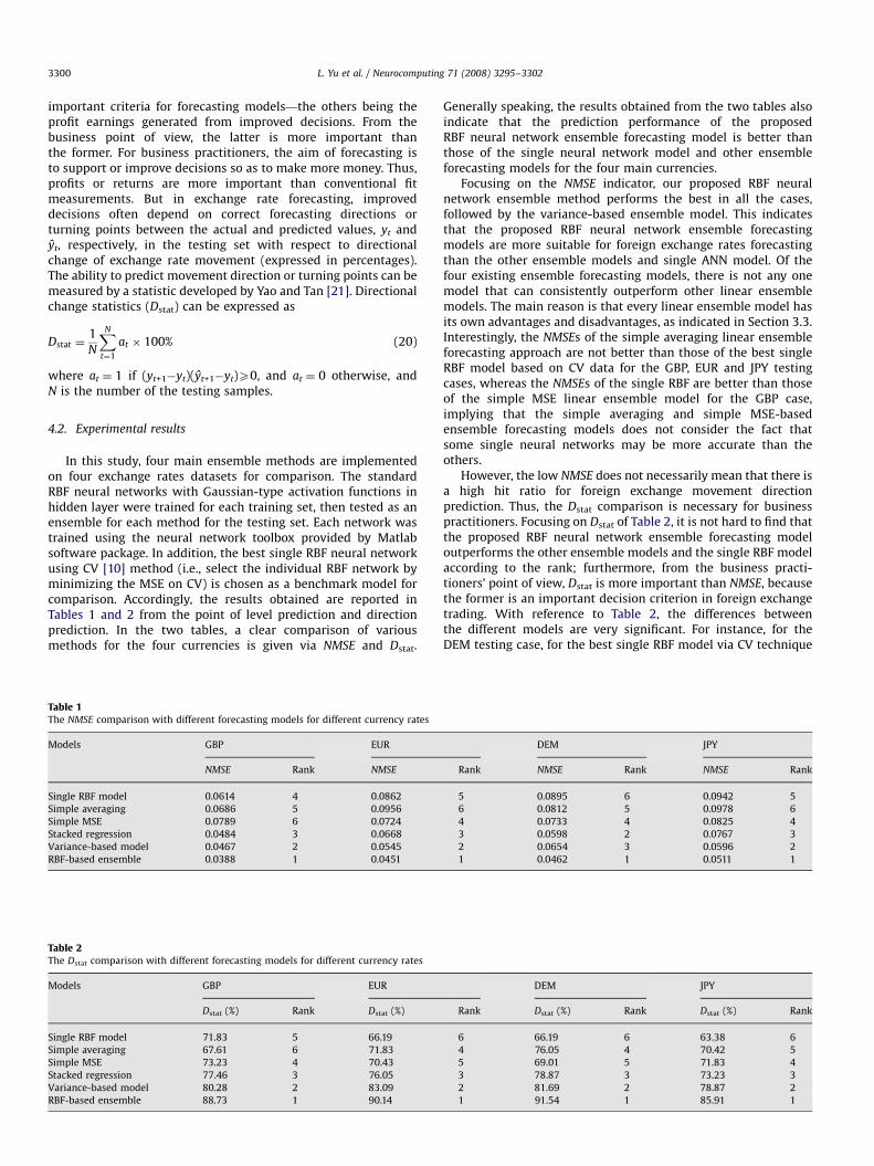
In this study, four main ensemble methods are implementedon four exchange rates datasets for comparison. The standardRBF neural networks with Gaussian-type activation functions inhidden layer were trained for each training set, then tested as anensemble for each method for the testing set. Each network wastrained using the neural network toolbox provided by Matlabsoftware package. In addition, the best single RBF neural networkusing CV [10] method (i.e., select the individual RBF network byminimizing the MSE on CV) is chosen as a benchmark model forcomparison. Accordingly, the results obtained are reported inTables 1 and 2 from the point of level prediction and directionprediction. In the two tables, a clear comparison of variousmethods for the four currencies is given via NMSE and Dstat.
Table 1The NMSE comparison with different forecasting models for different currency rates
Models GBP EUR
NMSE Rank NMSE
Single RBF model 0.0614 4 0.0862
Simple averaging 0.0686 5 0.0956
Simple MSE 0.0789 6 0.0724
Stacked regression 0.0484 3 0.0668
Variance-based model 0.0467 2 0.0545
RBF-based ensemble 0.0388 1 0.0451
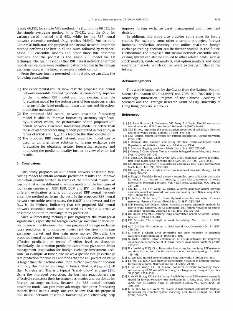
Table 2The Dstat comparison with different forecasting models for different currency rates
Models GBP EUR
Dstat (%) Rank Dstat (%)
Single RBF model 71.83 5 66.19
Simple averaging 67.61 6 71.83
Simple MSE 73.23 4 70.43
Stacked regression 77.46 3 76.05
Variance-based model 80.28 2 83.09
RBF-based ensemble 88.73 1 90.14
Generally speaking, the results obtained from the two tables alsoindicate that the prediction performance of the proposedRBF neural network ensemble forecasting model is better thanthose of the single neural network model and other ensembleforecasting models for the four main currencies.
Focusing on the NMSE indicator, our proposed RBF neuralnetwork ensemble method performs the best in all the cases,followed by the variance-based ensemble model. This indicatesthat the proposed RBF neural network ensemble forecastingmodels are more suitable for foreign exchange rates forecastingthan the other ensemble models and single ANN model. Of thefour existing ensemble forecasting models, there is not any onemodel that can consistently outperform other linear ensemblemodels. The main reason is that every linear ensemble model hasits own advantages and disadvantages, as indicated in Section 3.3.Interestingly, the NMSEs of the simple averaging linear ensembleforecasting approach are not better than those of the best singleRBF model based on CV data for the GBP, EUR and JPY testingcases, whereas the NMSEs of the single RBF are better than thoseof the simple MSE linear ensemble model for the GBP case,implying that the simple averaging and simple MSE-basedensemble forecasting models does not consider the fact thatsome single neural networks may be more accurate than theothers.
However, the low NMSE does not necessarily mean that there isa high hit ratio for foreign exchange movement directionprediction. Thus, the Dstat comparison is necessary for businesspractitioners. Focusing on Dstat of Table 2, it is not hard to find thatthe proposed RBF neural network ensemble forecasting modeloutperforms the other ensemble models and the single RBF modelaccording to the rank; furthermore, from the business practi-tioners’ point of view, Dstat is more important than NMSE, becausethe former is an important decision criterion in foreign exchangetrading. With reference to Table 2, the differences betweenthe different models are very significant. For instance, for theDEM testing case, for the best single RBF model via CV technique
DEM JPY
Rank NMSE Rank NMSE Rank
5 0.0895 6 0.0942 5
6 0.0812 5 0.0978 6
4 0.0733 4 0.0825 4
3 0.0598 2 0.0767 3
2 0.0654 3 0.0596 2
1 0.0462 1 0.0511 1
DEM JPY
Rank Dstat (%) Rank Dstat (%) Rank
6 66.19 6 63.38 6
4 76.05 4 70.42 5
5 69.01 5 71.83 4
3 78.87 3 73.23 3
2 81.69 2 78.87 2
1 91.54 1 85.91 1
ARTICLE IN PRESS
L. Yu et al. / Neurocomputing 71 (2008) 3295–3302 3301
is only 66.19%, for simple MSE method, the Dstat is only 69.01%, forthe simple averaging method, it is 76.05%, and the Dstat forvariance-based method is 81.69%, while for the RBF neuralnetwork ensemble method, Dstat reaches 91.54%. Furthermore,like NMSE indicator, the proposed RBF neural network ensemblemethod performs the best in all the cases, followed by variance-based RBF ensemble models and other three RBF ensemblemethods, and the poorest is the single RBF model via CVtechnique. The main reason is that RBF neural network ensemblemodels can capture some nonlinear patterns hidden in the foreignexchange rates, while linear ensemble models cannot.
From the experiments presented in this study, we can draw thefollowing conclusions
(1)
The experimental results show that the proposed RBF neuralnetwork ensemble forecasting model is consistently superiorto the individual RBF model and four existing ensembleforecasting model for the testing cases of four main currenciesin terms of the level-prediction measurement and direction-prediction measurement;(2)
The proposed RBF neural network ensemble forecastingmodel is able to improve forecasting accuracy significan-tly—in other words, the performance of the proposed RBFneural network ensemble forecasting model is better thanthose of all other forecasting models presented in this study interms of NMSE and Dstat. This leads to the third conclusion;(3)
The proposed RBF neural network ensemble model can beused as an alternative solution to foreign exchange rateforecasting for obtaining greater forecasting accuracy andimproving the prediction quality further in view of empiricalresults.5. Conclusions
This study proposes an RBF neural network ensemble fore-casting model to obtain accurate prediction results and improveprediction quality further. In terms of the empirical results, wecan find that across different ensemble models for the test cases offour main currencies—GBP, EUR, DEM and JPY—on the basis ofdifferent evaluation criteria, our proposed RBF neural networkensemble method performs the best. In the proposed RBF neuralnetwork ensemble testing cases, the NMSE is the lowest and theDstat is the highest, indicating that the proposed RBF neuralnetwork ensemble model can be used as a viable alternativeensemble solution to exchange rates prediction.
Such a forecasting technique just highlights the managerialsignificance, especially for foreign exchange investment decision.For business practitioners, the main purpose of foreign exchangerates prediction is to improve investment decision in foreignexchange market and thus gain more money. Obviously, theproposed neural network models in this study can produce a moreeffective prediction in terms of either level or direction.Particularly, the direction prediction can almost give some directmanagement implication for foreign exchange investment deci-sion. For example, at time t, one makes a specific foreign exchangerate prediction for time t+1 and finds that the t+1 prediction valueis larger than the t actual value, then his/her investment decisionis to buy this foreign exchange at time t. That is, if (xt+1�xt)40then buy else sell. This is a typical ‘‘trend-follow’’ strategy [21].Using the improved prediction, the business practitioners caneffectively construct their investment strategies and portfolios forforeign exchange markets. Because the RBF neural networkensemble model can gain more advantage than other forecastingmodels listed in this study, one can believe that the proposedRBF neural network ensemble forecasting can effectively help
improve foreign exchange asset management and investmentdecision.
In addition, this study also provides some clues for futurestudies. For example, some other ensemble strategies, forecasthorizons, prediction accuracy, and online real-time foreignexchange trading decision can be further studied in the future.Furthermore, the proposed RBF neural network ensemble fore-casting system can also be applied to other related fields, such asstock markets, crude oil markets, real option markets and someemerging markets, which can be worth exploring further in thefuture.
Acknowledgments
This work is supported by the Grants from the National NaturalScience Foundation of China (NSFC nos. 70601029, 70221001), theKnowledge Innovation Program of the Chinese Academy ofSciences and the Strategic Research Grant of City University ofHong Kong (SRG no. 7001677).
References
[1] J.A. Benediktsson, J.R. Sveinsson, O.K. Ersoy, P.H. Swain, Parallel consensualneural networks, IEEE Trans. Neural Networks 8 (1997) 54–64.
[2] C.M. Bishop, Improving the generalization properties of radial basis functionneural networks, Neural Comput. 3 (1991) 579–588.
[3] C.M. Bishop, Neural Networks for Pattern Recognition, Oxford UniversityPress, 1995.
[4] L. Breiman, Bias, variance, and arcing classifiers, Technical Report TR460,Department of Statistics, University of California, 1994.
[5] L. Breiman, Bagging predictors, Mach. Learn. 24 (1996) 123–140.[6] J. Carney, P. Cunningham, Tuning diversity in bagged ensembles, Int. J. Neural
Syst. 10 (2000) 267–280.[7] S. Chen, S.A. Billings, C.F.N. Cowan, P.M. Grant, Nonlinear systems identifica-
tion using radial basis functions, Int. J. Syst. Sci. 21 (1990) 2513–2539.[8] L.K. Hansen, P. Salamon, Neural network ensembles, IEEE Trans. Pattern Anal.
Mach. Intell. 12 (1990) 993–1001.[9] B.H. Kang, Unstable weights in the combination of forecasts, Manage. Sci. 32
(1986) 683–695.[10] A. Krogh, J. Vedelsby, Neural network ensembles, cross validation, and active
learning, in: G. Tesauro, D. Touretzky, T. Leen (Eds.), Advances in NeuralInformation Processing Systems, Vol. 7, MIT Press, Cambridge, MA, 1995, pp.231–238.
[11] K.K. Lai, L. Yu, S.Y. Wang, W. Huang, A novel nonlinear neural networkensemble model for financial time series forecasting, Lect. Notes Comput. Sci.1991 (2006) 790–793.
[12] U. Naftaly, N. Intrator, D. Horn, Optimal ensemble averaging of neuralnetworks, Network Comput. Neural Syst. 8 (1997) 283–296.
[13] M.P. Perrone, L.N. Cooper, When networks disagree: ensemble methods forhybrid neural networks, in: R.J. Mammone (Ed.), Neural Networks for Speechand Image Processing, Chapman & Hall, 1993, pp. 126–142.
[14] B.E. Rosen, Ensemble learning using decorrelated neural networks, Connec-tion Sci. 8 (1996) 373–384.
[15] R.E. Schapire, The strength of weak learnability, Mach. Learn. 5 (1990)197–227.
[16] A.J.C. Sharkey, On combining artificial neural nets, Connection Sci. 8 (1996)299–314.
[17] K. Tumer, J. Ghosh, Error correlation and error reduction in ensembleclassifiers, Connection Sci. 8 (1996) 385–404.
[18] N. Ueda, Optimal linear combination of neural networks for improvingclassification performance, IEEE Trans. Pattern Anal. Mach. Intell. 22 (2000)207–215.
[19] D.K. Wedding II, K.J. Cios, Time series forecasting by combining RBF networkscertainty factors and the Box-Jenkins model, Neurocomputing 10 (1996)149–168.
[20] D. Wolpert, Stacked generalization, Neural Networks 5 (1992) 241–259.[21] J.T. Yao, C.L. Tan, A case study on using neural networks to perform technical
forecasting of forex, Neurocomputing 34 (2000) 79–98.[22] L. Yu, S.Y. Wang, K.K. Lai, A novel nonlinear ensemble forecasting model
incorporating GLAR and ANN for foreign exchange rates, Comput. Oper. Res.32 (2005) 2523–2541.
[23] L. Yu, W. Huang, K.K. Lai, S.Y. Wang, A reliability-based RBF network ensemblemodel for foreign exchange rates prediction, in: I. King, et al. (Eds.), ICONIP2006, Part III, Lecture Notes in Computer Science, Vol. 4234, 2006, pp.380–389.
[24] L. Yu, K.K. Lai, S.Y. Wang, W. Huang, A bias-variance-complexity trade-offframework for complex system modeling, Lect. Notes Comput. Sci. 3980(2006) 518–527.

ARTICLE IN PRESS
L. Yu et al. / Neurocomputing 71 (2008) 3295–33023302
Lean Yu received the Ph.D. degree in ManagementSciences and Engineering from the Academy of Mathe-matics and Systems Science, Chinese Academy ofSciences (CAS), Beijing in 2005. He has published morethan 30 papers in journals including IEEE Transactionson Knowledge and Data Engineering, European Journalof Operational Research, International Journal ofIntelligent Systems, and Computers & OperationsResearch. He is currently an associate professor in theAcademy of Mathematics and Systems Science ofChinese Academy of Sciences. His research interestsinclude artificial intelligent system, computer simula-tion, decision support systems, knowledge manage-
ment and financial forecasting.K. K. Lai is the Chair Professor of Management Scienceat City University of Hong Kong, and he is also theAssociate Dean of the Faculty of Business. Currently, heis also acting as the Dean of College of BusinessAdministration at Hunan University, China. Prior to hiscurrent post, he was a Senior Operational ResearchAnalyst at Cathay Pacific Airways and the AreaManager on Marketing Information Systems at UnionCarbide Eastern. Professor Lai received his Ph.D. atMichigan State University, USA. Professor Lai’s mainresearch interests include logistics and operationsmanagement, computer simulation, AI and business
decision modeling.Shouyang Wang received the Ph.D. degree in Opera-tions Research from Institute of Systems Science,Chinese Academy of Sciences (CAS), Beijing in 1986.He is currently a Bairen distinguished professor ofManagement Science at Academy of Mathematics andSystems Sciences of CAS and a Lotus chair professor ofHunan University, Changsha. He is the editor-in-chiefor a co-editor of 12 journals. He has published 18 booksand over 120 journal papers. His current researchinterests include financial engineering, e-auctions anddecision support systems.


