
Multinomial logistic regression
Azmi Mohd Tamil

Extension of Binary Logistic Regression• Multinomial logistic regression is the extension for
the (binary) logistic regression when the categorical dependent outcome has more than two levels.
• For example, instead of predicting only • dead or
• alive,
• we may have three groups, namely: • dead,
• lost to follow-up, and
• alive.
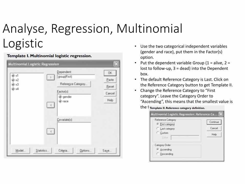
Analyse, Regression, Multinomial Logistic • Use the two categorical independent variables
(gender and race), put them in the Factor(s) option.
• Put the dependent variable Group (1 = alive, 2 = lost to follow-up, 3 = dead) into the Dependent box.
• The default Reference Category is Last. Click on the Reference Category button to get Template II.
• Change the Reference Category to “First category”. Leave the Category Order to “Ascending”, this means that the smallest value is the first category.

Model Options
• The Main effects option will include all the variables specified with no interaction terms whereas the Full factorial option will provide the main effects with all possible interactions.
• For the Custom/Stepwise option, we have a choice to set up the relevant main effects and interaction terms using the Forced Entry option or to perform a Stepwise analysis.
• Let us use the Main effects option.

Further Options
Results
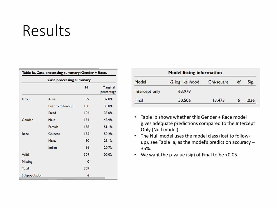
• Table Ib shows whether this Gender + Race model gives adequate predictions compared to the Intercept Only (Null model).
• The Null model uses the model class (lost to follow-up), see Table Ia, as the model’s prediction accuracy –35%.
• We want the p-value (sig) of Final to be <0.05.
Results
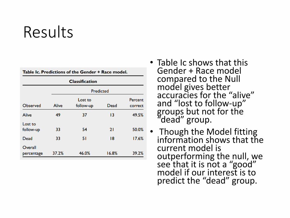
• Table Ic shows that this Gender + Race model compared to the Null model gives better accuracies for the “alive” and “lost to follow-up” groups but not for the “dead” group.
• Though the Model fitting information shows that the current model is outperforming the null, we see that it is not a “good” model if our interest is to predict the “dead” group.
Results
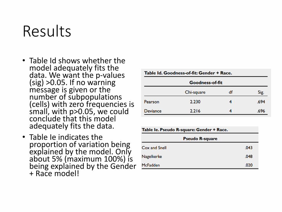
• Table Id shows whether the model adequately fits the data. We want the p-values (sig) >0.05. If no warning message is given or the number of subpopulations (cells) with zero frequencies is small, with p>0.05, we could conclude that this model adequately fits the data.
• Table Ie indicates the proportion of variation being explained by the model. Only about 5% (maximum 100%) is being explained by the Gender + Race model!

Results
• The Likelihood ratio test (Table If) shows the contribution of each variable to the model –Gender had a significant (p<0.05) contribution but not Race.
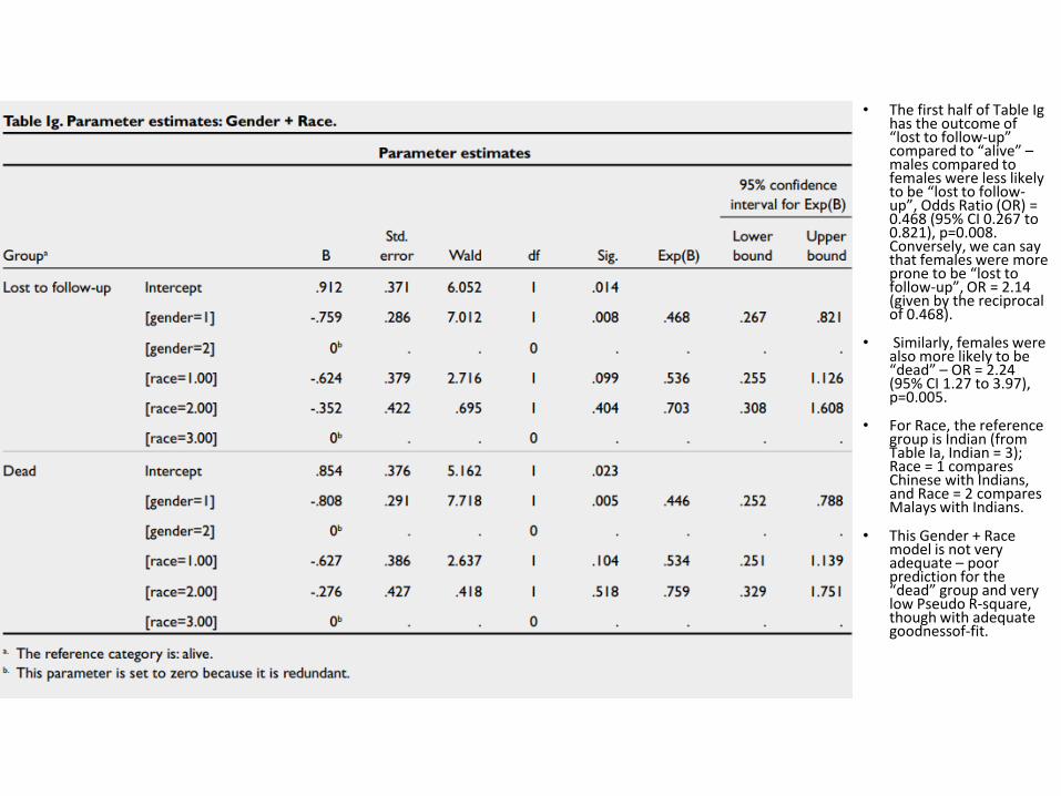
• The first half of Table Ig has the outcome of “lost to follow-up” compared to “alive” –males compared to females were less likely to be “lost to follow-up”, Odds Ratio (OR) = 0.468 (95% CI 0.267 to 0.821), p=0.008. Conversely, we can say that females were more prone to be “lost to follow-up”, OR = 2.14 (given by the reciprocal of 0.468).
• Similarly, females were also more likely to be “dead” – OR = 2.24 (95% CI 1.27 to 3.97), p=0.005.
• For Race, the reference group is Indian (from Table Ia, Indian = 3); Race = 1 compares Chinese with Indians, and Race = 2 compares Malays with Indians.
• This Gender + Race model is not very adequate – poor prediction for the “dead” group and very low Pseudo R-square, though with adequate goodnessof-fit.
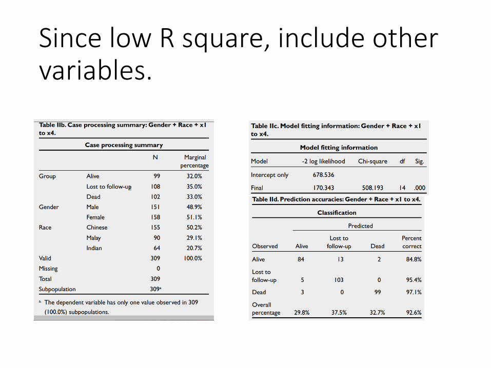
Since low R square, include other variables.
Results

Results
• Significant contributors to the model are x1 and x2 (Table IIg).
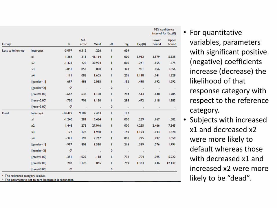
• For quantitative variables, parameters with significant positive (negative) coefficients increase (decrease) the likelihood of that response category with respect to the reference category.
• Subjects with increased x1 and decreased x2 were more likely to default whereas those with decreased x1 and increased x2 were more likely to be “dead”.


