Download - Maureen O'Leary
IMAGING WITH DIFFUSE PHOTON DENSITY WAVES
Maureen A. O'Leary
A DISSERTATION
in
PHYSICS
Presented to the Faculties of the University of Pennsylvania in Partial Ful�llment of
the Requirements for the Degree of Doctor of Philosophy
1996
Arjun G. Yodh
Supervisor of Dissertation
Robert Hollebeek
Graduate Group Chairperson
COPYRIGHT
Maureen Ann O'Leary
1996
DEDICATION
This work is dedicated to
Mom, Dad,
Terry, Stephen, Kathleen,
and Surge.
iii
ACKNOWLEDGEMENTS
Because my project has straddled the mutually exclusive worlds of Penn physics
and Penn biophysics, it has been my privilege to have had the guidance of two ad-
visors, Dr. Britton Chance from the Biochemistry and Biophysics Department, and
Dr. Arjun Yodh from the Physics department.
Arjun Yodh provided me with many of the ideas and helped me learn the physics I
needed to solve some di�cult problems. I thank him for the many nights and weekends
he spent helping me with papers and presentations. In the physics department I took
my courses, and exams, and defended this thesis. Dr. Ralf Amado has been a constant
support throughout this process. Tony Dinsmore, Peter Kaplan and especially Xingde
Li, have been valuable coworkers from the physics department.
But it was in the Department of Biochemistry and Biophysics that I �nally felt at
home. I thank Dr. Les Dutton for supporting me on his training grant and allowing
me to work in his lab. He introduced me to the Biochemistry and Biophysics depart-
ment, where both men and women can enjoy scienti�c inquiry without intimidation.
He also introduced me to my second advisor, Dr. Britton Chance. Britton Chance,
besides being a scienti�c and athletic legend, is an incredibly supportive advisor and
does his best to advance everyone around him. Britton gave me the opportunity to
speak at many meetings, and made me known to some of the most in uential people
in research today.
I also thank him for setting up a terri�c group of people who are part of the
lab. Although this list is no where near complete, it has been a pleasure to work
with Hanli Liu, Shoko Nioka, Mary Leonard, Dot Colemna, Shiyin Zhao, and Henry
Williams. Libo He, Ben Duggan and Jian Weng taught me all I needed to know about
electronics.
It has been my honor, to have had the opportunity to work for four years with
David Boas. Besides being the greatest scientist that I have ever known, he is a good
friend and an enthusiastic coworker. Without David, this project would not have been
the success that it was, and I probably would not have had the strength to �nish it
iv

Acknowledgements v
without David's support.
ABSTRACT
IMAGING WITH DIFFUSE PHOTON DENSITY WAVES
Maureen A. O'Leary
Arjun G. Yodh
Di�using photons can be used to probe and characterize optically thick turbid sam-
ples such as paints, foams and human tissue. In this work, we present experiments
which illustrate the properties of di�use photon density waves. Our observations
demonstrate the manipulation of these waves by adjustment of the photon di�usion
coe�cients of adjacent media. The waves are imaged, and are shown to obey simple
relations such as Snell's Law.
Next we present images of heterogeneous turbid media derived frommeasurements
of di�use photon density waves. These images are the �rst experimental reconstruc-
tions based on frequency-domain optical tomography. We demonstrate images of both
absorbing and scattering homogeneities, and show that this method is sensitive to the
optical properties of a heterogeneity. The algorithm employs a di�erential measure-
ment scheme which reduces the e�ect of errors resulting from incorrect estimations
of the background optical properties.
In addition to imaging absorption and scattering changes, we are also able to
image the lifetime and concentration pro�le of heterogeneous uorescent media.
vi
Contents
1 Introduction 1
1.1 Historical Perspective : : : : : : : : : : : : : : : : : : : : : : : : : : : 2
1.2 Photon Di�usion Equation : : : : : : : : : : : : : : : : : : : : : : : : 5
1.3 Introduction to Optical Imaging : : : : : : : : : : : : : : : : : : : : : 6
1.3.1 Forward Models : : : : : : : : : : : : : : : : : : : : : : : : : : 6
1.3.2 The Inverse Problem : : : : : : : : : : : : : : : : : : : : : : : 10
1.4 Resolution : : : : : : : : : : : : : : : : : : : : : : : : : : : : : : : : : 11
1.5 Contrast : : : : : : : : : : : : : : : : : : : : : : : : : : : : : : : : : : 13
2 Optics for Di�use Photon Density Waves 17
3 Hardware Speci�cations 33
3.1 Photon Detection - Photomultiplier tubes : : : : : : : : : : : : : : : 34
3.2 Photon Detection - Avalanche Photodiodes : : : : : : : : : : : : : : : 39
3.3 Laser diodes : : : : : : : : : : : : : : : : : : : : : : : : : : : : : : : : 42
3.4 Amplitude-phase detector : : : : : : : : : : : : : : : : : : : : : : : : 44
3.5 Signal Generators : : : : : : : : : : : : : : : : : : : : : : : : : : : : : 46
3.6 Filters : : : : : : : : : : : : : : : : : : : : : : : : : : : : : : : : : : : 47
3.7 Mixers : : : : : : : : : : : : : : : : : : : : : : : : : : : : : : : : : : : 51
3.8 Summary : : : : : : : : : : : : : : : : : : : : : : : : : : : : : : : : : 51
4 Imaging the Absorption Coe�cient 55
4.1 The Heterogeneous Di�usion Equation : : : : : : : : : : : : : : : : : 56
vii
viii O'Leary, Imaging with Di�use Photon Density Waves
4.2 Born Approximation : : : : : : : : : : : : : : : : : : : : : : : : : : : 56
4.3 Rytov Approximation : : : : : : : : : : : : : : : : : : : : : : : : : : : 58
4.4 Breakdown of the Born and Rytov Approximations : : : : : : : : : : 59
4.5 Inverting the Solutions to the Heterogeneous Di�usion Equation : : : 60
4.6 Singular Value Decomposition : : : : : : : : : : : : : : : : : : : : : : 64
4.7 Algebraic Reconstruction Techniques : : : : : : : : : : : : : : : : : : 69
4.8 Data Analysis : : : : : : : : : : : : : : : : : : : : : : : : : : : : : : : 72
4.9 Experimental and Computational Results : : : : : : : : : : : : : : : : 79
4.10 Updating the Weight Functions : : : : : : : : : : : : : : : : : : : : : 80
4.11 Resolving Multiple Objects : : : : : : : : : : : : : : : : : : : : : : : : 83
4.12 DPDW Imaging Combined With Other Imaging Modalities : : : : : 84
4.13 Finite Systems : : : : : : : : : : : : : : : : : : : : : : : : : : : : : : 92
5 Imaging the Scattering coe�cient 95
5.1 Born Expansion : : : : : : : : : : : : : : : : : : : : : : : : : : : : : : 96
5.2 Rytov Expansion : : : : : : : : : : : : : : : : : : : : : : : : : : : : : 97
5.3 Matrix Equations : : : : : : : : : : : : : : : : : : : : : : : : : : : : : 101
6 Absorption and Scattering 105
6.1 Simulation Results : : : : : : : : : : : : : : : : : : : : : : : : : : : : 106
7 Imaging Fluorescence 111
7.1 Fluorescent Di�use Photon Density Wave Theory : : : : : : : : : : : 112
7.2 Localizing Fluorescent Objects : : : : : : : : : : : : : : : : : : : : : : 116
7.3 Tomographic Imaging of Fluorescent Objects : : : : : : : : : : : : : : 123
8 Summary 133
A Singular Matrices 135
B Time Resolved Spectroscopy 137
ix
C Time Domain Fluorescent DPDW Derivation 141
D Back Projection 143
E The Photon Migration Imaging Software Package 147
E.1 Sample PMI scripts : : : : : : : : : : : : : : : : : : : : : : : : : : : : 149
E.2 PMI Command Summary : : : : : : : : : : : : : : : : : : : : : : : : 152
F Parallel Processing 177
List of Figures
1.1 Absorption spectra of major tissue chromophores. : : : : : : : : : : : 3
1.2 A simpli�ed schematic of the RunManTM instrument. : : : : : : : : : 4
1.3 A typical RunManTM oxygenation trace : : : : : : : : : : : : : : : : 4
1.4 A reconstruction of two absorbing objects : : : : : : : : : : : : : : : 7
1.5 Sample weight distributions for CAT and di�use photon imaging. : : 8
1.6 Sample weight distributions for a pulsed source on the surface of a
semi-in�nite medium. : : : : : : : : : : : : : : : : : : : : : : : : : : : 9
2.1 Experimental DPDW phase contours. : : : : : : : : : : : : : : : : : : 24
2.2 Refraction of DPDW's. : : : : : : : : : : : : : : : : : : : : : : : : : : 27
2.3 Refraction by a spherical surface : : : : : : : : : : : : : : : : : : : : : 28
2.4 The amplitude and phase of a simulated phased array : : : : : : : : : 29
2.5 The amplitude and phase of scanned phased array : : : : : : : : : : : 30
2.6 Three possible con�gurations for the phased array measurements. : : 31
3.1 A schematic of the frequency domain instrument. : : : : : : : : : : : 34
3.2 The spectral sensitivity and quantum e�ciency of the R928 PMT. : : 36
3.3 Experimental setup for testing the amplitude-phase cross-talk of the
PMT. : : : : : : : : : : : : : : : : : : : : : : : : : : : : : : : : : : : 37
3.4 The dynode structure and position sensitivity of the R928 PMT. : : : 38
3.5 Holding the DC current from the PMT constant reduces the amplitude-
phase cross-talk. : : : : : : : : : : : : : : : : : : : : : : : : : : : : : : 39
3.6 The current versus voltage curve of an ideal zener diode. : : : : : : : 39
3.7 A Zener diode is used to reduce the space-charge e�ect on the phase. 40
x
xi
3.8 Schematic of a silicon photo-diode. : : : : : : : : : : : : : : : : : : : 42
3.9 The spectral sensitivity and quantum e�ciency of the photodiode in
an APD. : : : : : : : : : : : : : : : : : : : : : : : : : : : : : : : : : : 43
3.10 An AC signal is capacitor coupled to the laser diode driving current. : 44
3.11 A schematic of the lock-in ampli�er. : : : : : : : : : : : : : : : : : : : 45
3.12 Amplitude-phase cross-talk of the SRS530. : : : : : : : : : : : : : : : 47
3.13 Twin-T bandpass �lter. : : : : : : : : : : : : : : : : : : : : : : : : : : 48
3.14 The response of the twin-T band-pass �lter at several di�erent Q. : : 49
3.15 Amplitude-phase cross-talk of the twin-T �lter : : : : : : : : : : : : : 49
3.16 RLC bandpass �lter. : : : : : : : : : : : : : : : : : : : : : : : : : : : 50
3.17 Amplitude-phase cross-talk of the RLC �lter : : : : : : : : : : : : : : 50
3.18 Schematics of sample mixers. : : : : : : : : : : : : : : : : : : : : : : 52
4.1 Schematic of the Born solution to the heterogeneous di�usion equation. 58
4.2 A comparison of the Born and Rytov approximations. : : : : : : : : : 60
4.3 A typical scanning geometry and volume digitization. : : : : : : : : : 62
4.4 Linear algebra de�nitions for SVD : : : : : : : : : : : : : : : : : : : : 66
4.5 Eigenvalue smoothing algorithm for singular value decomposition : : 68
4.6 Algebraic reconstruction : : : : : : : : : : : : : : : : : : : : : : : : : 70
4.7 Algebraic reconstruction using noisy or incomplete data : : : : : : : : 71
4.8 Reconstructed absorption images as a function of SIRT iteration : : : 72
4.9 Geometry of the reference measurements. : : : : : : : : : : : : : : : : 74
4.10 Reconstructions of absorption when the background absorption is mis-
estimated - no SIRT constraints. : : : : : : : : : : : : : : : : : : : : : 77
4.11 Reconstructions of absorption when the background absorption is mis-
estimated - with SIRT constraints. : : : : : : : : : : : : : : : : : : : 78
4.12 Reconstruction of a single perfect absorber. : : : : : : : : : : : : : : : 80
4.13 Reconstruction of a series of absorbing spheres. : : : : : : : : : : : : 81
4.14 Resolution of two absorbing spheres : : : : : : : : : : : : : : : : : : : 85
4.15 An overly simpli�ed breast model. : : : : : : : : : : : : : : : : : : : : 86
xii O'Leary, Imaging with Di�use Photon Density Waves
4.16 1st and 2nd iteration of reconstructed absorption versus the true value,
for a single spherical inhomogeneity. : : : : : : : : : : : : : : : : : : : 89
4.17 Simulation with six absorbing inhomogeneities. : : : : : : : : : : : : 89
4.18 A tissue phantom simulating a human breast : : : : : : : : : : : : : : 91
4.19 A schematic of the image sources and image objects needed to model
a semi-in�nite boundary condition. : : : : : : : : : : : : : : : : : : : 93
5.1 The reconstruction of a highly scattering sphere. : : : : : : : : : : : : 102
5.2 Reconstructed scattering images as a function of SIRT iteration : : : 103
6.1 Simultaneous reconstructions of absorption and scattering. : : : : : : 108
6.2 E�ect of absorption versus scattering variation on amplitude and phase.109
6.3 Reconstruction of absorption and scattering using amplitude and/or
phase data : : : : : : : : : : : : : : : : : : : : : : : : : : : : : : : : : 110
7.1 A schematic of uorescent DPDW generation. : : : : : : : : : : : : : 115
7.2 Experimental measurements of uorescent di�use photon density waves.118
7.3 Experimentalmeasurements of uorescent di�use photon density waves
from a cylindrical object. : : : : : : : : : : : : : : : : : : : : : : : : : 118
7.4 A device for localizing the center of a uorescent object. : : : : : : : 120
7.5 The estimated position of a reradiator using the �tting algorithm. : : 121
7.6 Localization of a uorescent object using a phased array. : : : : : : : 122
7.7 Images proportional to uorophore concentration show spurious voxels
with unphysical optical properties. : : : : : : : : : : : : : : : : : : : 126
7.8 A plot of tan�1(!� ) versus !� shows the saturation e�ect for !� greater
than 1. : : : : : : : : : : : : : : : : : : : : : : : : : : : : : : : : : : 127
7.9 Reconstruction of uorophore lifetime and concentration in a system
with no background uorophore. : : : : : : : : : : : : : : : : : : : : 128
7.10 A cartoon describing the breakdown of the background uorescence
problem. : : : : : : : : : : : : : : : : : : : : : : : : : : : : : : : : : : 129
xiii
7.11 Reconstruction of uorophore lifetime and concentration in a system
with background uorophore. : : : : : : : : : : : : : : : : : : : : : : 131
B.1 A schematic of the TRS system : : : : : : : : : : : : : : : : : : : : : 138
B.2 Signal processing by the constant fraction discriminator (CFD) : : : : 138
B.3 Equivalent circuit for the time amplitude converter (TAC). : : : : : : 138
D.1 The measurement geometry for the NIM back-projection imaging project.145
D.2 Sample back-projection images for a solid block sample with an em-
bedded heterogeneity. : : : : : : : : : : : : : : : : : : : : : : : : : : : 145
F.1 An overview of the PMI software : : : : : : : : : : : : : : : : : : : : 178
F.2 A block diagram of the ow of the parallel code. : : : : : : : : : : : : 179
F.3 The CPU times for various homogeneous and heterogeneous systems. 181
List of Tables
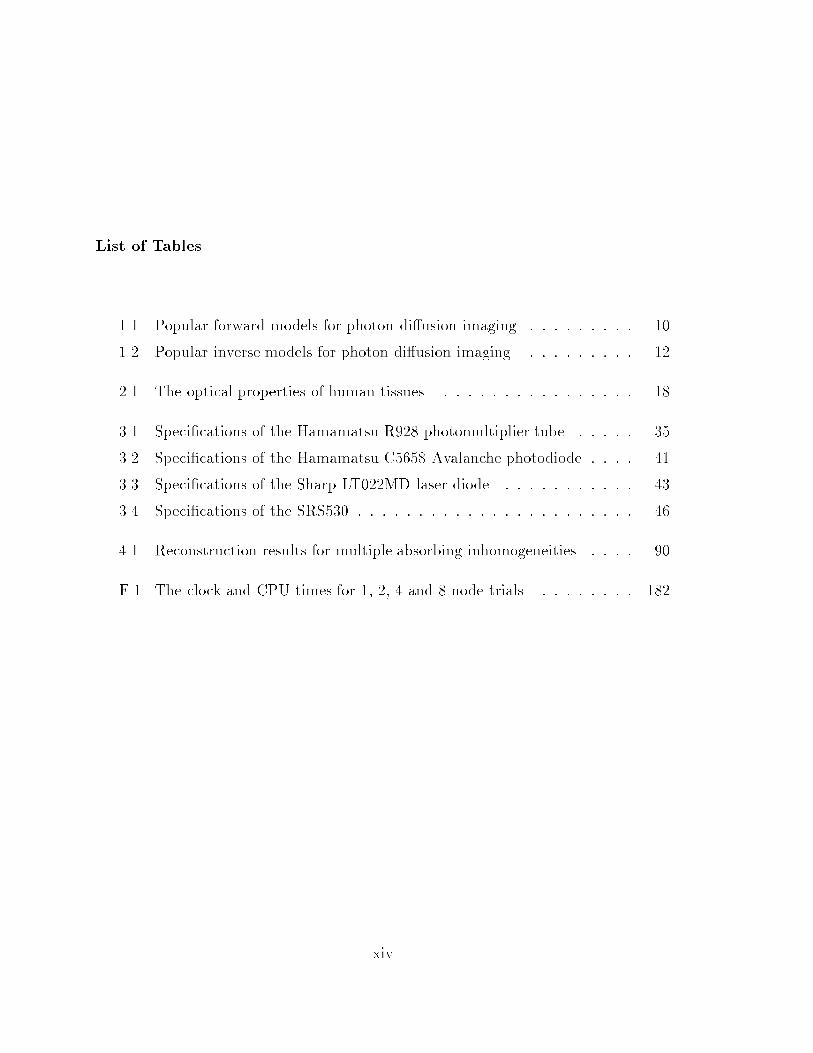
1.1 Popular forward models for photon di�usion imaging. : : : : : : : : : 10
1.2 Popular inverse models for photon di�usion imaging. : : : : : : : : : 12
2.1 The optical properties of human tissues. : : : : : : : : : : : : : : : : 18
3.1 Speci�cations of the Hamamatsu R928 photomultiplier tube. : : : : : 35
3.2 Speci�cations of the Hamamatsu C5658 Avalanche photodiode. : : : : 41
3.3 Speci�cations of the Sharp LT022MD laser diode. : : : : : : : : : : : 43
3.4 Speci�cations of the SRS530 : : : : : : : : : : : : : : : : : : : : : : : 46
4.1 Reconstruction results for multiple absorbing inhomogeneities. : : : : 90
F.1 The clock and CPU times for 1, 2, 4 and 8 node trials. : : : : : : : : 182
xiv
Chapter 1
Introduction
In this work, we will explore how light travels through highly scattering media. Al-
though we are primarily concerned with light di�usion through tissue for medical
diagnostic purposes, there are many applications of interest. For example, clouds,
paint and foams are all highly scattering media. We model the transport of light
through the media as a di�usion process. The analysis used here can be applied
to other di�usional processes such as heat di�usion, neutron di�usion, or chemical
di�usion.
In this chapter we will brie y review some uses of light in medical diagnostics.
Next we will give an overview of di�use photon imaging. As in most imaging tech-
niques, creation of an image requires an understanding of the interaction between
the probe and the media (i.e. the forward model). The forward model relates a
measurement to the optical properties of the medium. When the forward problem is
well understood, a series of measurements are made, and �nally, the measurements
and the forward model are used together to derive a map of the properties of the
medium (i.e. the inverse problem). We will outline some popular forward models and
inversion methods, and discuss the resolution of di�usive wave based optical imaging
and the types of contrasts measurable using optical probes.
1
2 O'Leary, Imaging with Di�use Photon Density Waves
1.1 Historical Perspective
As early as 1929, researchers investigated passing bright light through the body to cre-
ate shadow images [1]. These transillumination images were of poor quality because
light is multiply scattered as it passes through tissue, and it is di�cult to separate
scattering e�ects from absorption e�ects. In the past 20 years, a better understand-
ing of how photons travel through tissue has enabled researchers to correlate internal
physiological changes to optical changes. We and other investigators have begun to
image the these optical changes using a variety of methods.
As the diagnostic power of optical measurements is improved, optical measure-
ments are be expected to gain wider acceptance within the medical community. Re-
cent technological developments a�ord the possibility of compact, low cost medical
optical instruments In low power (less than 100 mW peak power) near infra-red stud-
ies, the developments include light emitting diodes and laser diodes, which replace
table top laser systems used in research laboratories, and solid state detectors such
as the avalanche photodiode which have a fast response time and broad spectral
sensitivity.
Most medical optical instruments use single scattering to probe tissue at or near
its surface. Laser Doppler ow-meters and angiograms are examples of near surface
measurements. In this work we are interested in developing instruments which probe
more deeply (3 - 10 cm) into the tissue.
An example of an instrument which uses multiply scattered light is the �nger pulse
meter. Here the amount of light which passes through a patient's �nger changes as
blood pressure causes vessels to expand and contract. As the �nger �lls with blood
and expands, the amount of transmitted light decreases. This change in transmission
is currently used to continuously, and non-invasively monitor the pulse rate of many
intensive care patients.
An improvement to the pulse meter introduces the use of spectral �lters to com-
pare light transmission at di�erent wavelengths. If we examine the water absorption
spectra of the major tissue chromophores (�gure 1.1), we see that in the near infra-
Introduction 3
WAVELENGTH (nm)
Deoxy Hb
Water0.25
700 800 900 1000
0.30
0.20
0.15
0.10
0.05
0.00
600 1100
Oxy Hb
AB
SOR
PT
ION
CO
EF
ICIE
NT
(1/
cm)
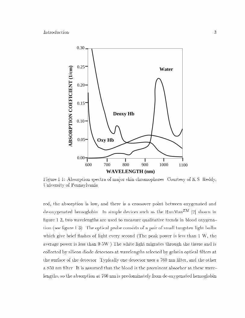
Figure 1.1: Absorption spectra of major skin chromophores. Courtesy of K.S. Reddy,University of Pennsylvania.
red, the absorption is low, and there is a crossover point between oxygenated and
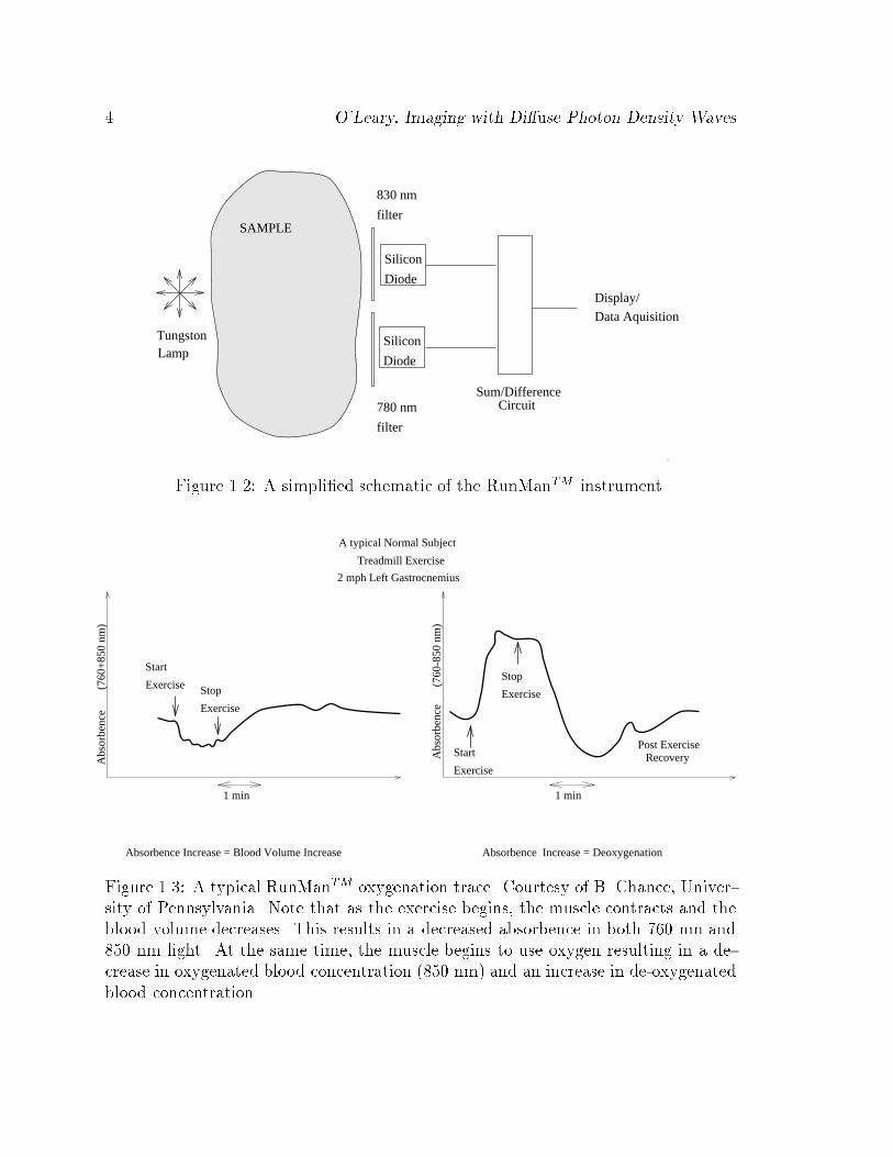
de-oxygenated hemoglobin. In simple devices such as the RunManTM [2] shown in
�gure 1.2, two wavelengths are used to measure qualitative trends in blood oxygena-
tion (see �gure 1.3). The optical probe consists of a pair of small tungsten light bulbs
which give brief ashes of light every second (The peak power is less than 1 W, the
average power is less than 0.5W.) The white light migrates through the tissue and is
collected by silicon diode detectors at wavelengths selected by gelatin optical �lters at
the surface of the detector. Typically one detector uses a 760 nm �lter, and the other
a 850 nm �lter. It is assumed that the blood is the prominent absorber at these wave-
lengths, so the absorption at 760 nm is predominately from de-oxygenated hemoglobin
4 O'Leary, Imaging with Di�use Photon Density Waves
Diode
Silicon
Circuit
LampTungston
Diode
Sum/Difference
Silicon
filter
780 nm
filter
830 nm
Display/
Data Aquisition
SAMPLE
Figure 1.2: A simpli�ed schematic of the RunManTM instrument.
Stop
ExerciseStop
Exercise
Start
Exercise
Start
Exercise
Treadmill Exercise
A typical Normal Subject
2 mph Left Gastrocnemius
Post ExerciseRecovery
1 min 1 min
Absorbence Increase = Blood Volume Increase
(760
-850
nm
)
(760
+85
0 nm
)
Absorbence Increase = Deoxygenation
Abs
orbe
nce
Abs
orbe
nce
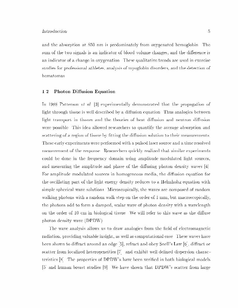
Figure 1.3: A typical RunManTM oxygenation trace. Courtesy of B. Chance, Univer-sity of Pennsylvania. Note that as the exercise begins, the muscle contracts and the
blood volume decreases. This results in a decreased absorbence in both 760 nm and
850 nm light. At the same time, the muscle begins to use oxygen resulting in a de-crease in oxygenated blood concentration (850 nm) and an increase in de-oxygenated
blood concentration.
Introduction 5
and the absorption at 850 nm is predominately from oxygenated hemoglobin. The
sum of the two signals is an indicator of blood volume changes, and the di�erence is
an indicator of a change in oxygenation. These qualitative trends are used in exercise
studies for professional athletes, analysis of myoglobin disorders, and the detection of
hematomas.
1.2 Photon Di�usion Equation
In 1988 Patterson et al. [3] experimentally demonstrated that the propagation of
light through tissue is well described by a di�usion equation. Thus analogies between
light transport in tissues and the theories of heat di�usion and neutron di�usion
were possible. This idea allowed researchers to quantify the average absorption and
scattering of a region of tissue by �tting the di�usion solution to their measurements.
These early experimentswere performed with a pulsed laser source and a time resolved
measurement of the response. Researchers quickly realized that similar experiments
could be done in the frequency domain using amplitude modulated light sources,
and measuring the amplitude and phase of the di�using photon density waves [4].
For amplitude modulated sources in homogeneous media, the di�usion equation for
the oscillating part of the light energy density reduces to a Helmholtz equation with
simple spherical wave solutions. Microscopically, the waves are composed of random
walking photons with a random walk step on the order of 1 mm, but macroscopically,
the photons add to form a damped, scalar wave of photon density with a wavelength
on the order of 10 cm in biological tissue. We will refer to this wave as the di�use
photon density wave (DPDW).
The wave analysis allows us to draw analogies from the �eld of electromagnetic
radiation, providing valuable insight, as well as computational ease. These waves have
been shown to di�ract around an edge [5], refract and obey Snell's Law [6], di�ract or
scatter from localized heterogeneities [7]. and exhibit well de�ned dispersion charac-
teristics [8]. The properties of DPDW's have been veri�ed in both biological models
[5] and human breast studies [9]. We have shown that DPDW's scatter from large
6 O'Leary, Imaging with Di�use Photon Density Waves
spherical inhomogeneities in a way that is similar to, but simpler than, Mie scattering
[10]; and that DPDW's in a uorescent medium are absorbed and then re-radiated
creating uorescent DPDW's whose wavelengths are governed by the optical proper-
ties of the medium at the Stoke-shifted optical wavelength [7, 11, 12].
1.3 Introduction to Optical Imaging
Since the advent of the photon di�usion equation, researchers have struggled to ac-
curately measure the optical properties of biological systems. For example, the head
is made up of blood, white matter, grey matter, bone, skin, etc. Each of these types
of tissues has di�erent optical properties. If one assumes a homogeneous model to
calculate the average optical properties, one cannot obtain accurate values for the ab-
sorption and the scattering. Instead, an average value of the tissue optical properties
is derived. Thus, there has been a great deal of interest in creating a quantitative map
or \image" of the optical properties. In particular, physicians are interested in func-
tional imaging and the localization and characterization of tumors and hematomas.
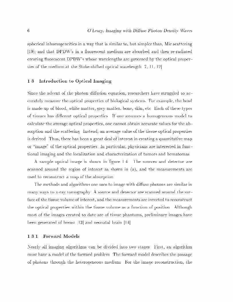
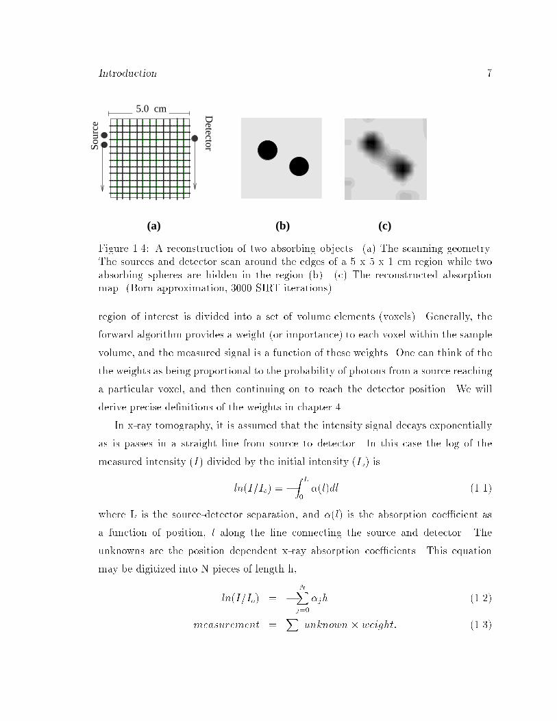
A sample optical image is shown in �gure 1.4. The sources and detector are
scanned around the region of interest as shown in (a), and the measurements are
used to reconstruct a map of the absorption.
The methods and algorithms one uses to image with di�use photons are similar in
many ways to x-ray tomography. A source and detector are scanned around the sur-
face of the tissue volume of interest, and the measurements are inverted to reconstruct
the optical properties within the tissue volume as a function of position. Although
most of the images created to date are of tissue phantoms, preliminary images have
been generated of breast [13] and neonatal brain [14].
1.3.1 Forward Models
Nearly all imaging algorithms can be divided into two stages. First, an algorithm
must have a model of the forward problem. The forward model describes the passage
of photons through the heterogeneous medium. For the image reconstruction, the
Introduction 7
(a) (c)(b)
5.0 cm
Sour
ce
Detector
Figure 1.4: A reconstruction of two absorbing objects. (a) The scanning geometry.The sources and detector scan around the edges of a 5 x 5 x 1 cm region while two
absorbing spheres are hidden in the region (b). (c) The reconstructed absorptionmap. (Born approximation, 3000 SIRT iterations)
region of interest is divided into a set of volume elements (voxels). Generally, the
forward algorithm provides a weight (or importance) to each voxel within the sample
volume, and the measured signal is a function of these weights. One can think of the
the weights as being proportional to the probability of photons from a source reaching
a particular voxel, and then continuing on to reach the detector position. We will
derive precise de�nitions of the weights in chapter 4.
In x-ray tomography, it is assumed that the intensity signal decays exponentially
as is passes in a straight line from source to detector. In this case the log of the
measured intensity (I) divided by the initial intensity (Io) is
ln(I=Io) = �Z L
0
�(l)dl (1.1)
where L is the source-detector separation, and �(l) is the absorption coe�cient as
a function of position, l along the line connecting the source and detector. The
unknowns are the position dependent x-ray absorption coe�cients. This equation
may be digitized into N pieces of length h,
ln(I=Io) = �
NXj=0
�jh (1.2)
measurement =X
unknown � weight: (1.3)
8 O'Leary, Imaging with Di�use Photon Density Waves
DetectorDetector
Source Source
0
−β
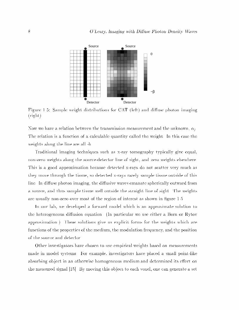
Figure 1.5: Sample weight distributions for CAT (left) and di�use photon imaging(right).
Now we have a relation between the transmission measurement and the unknown, �j.
The relation is a function of a calculable quantity called the weight. In this case the
weights along the line are all -h.
Traditional imaging techniques such as x-ray tomography typically give equal,
non-zero weights along the source-detector line of sight, and zero weights elsewhere.
This is a good approximation because detected x-rays do not scatter very much as
they move through the tissue, so detected x-rays rarely sample tissue outside of this
line. In di�use photon imaging, the di�usive waves emanate spherically outward from
a source, and thus sample tissue well outside the straight line of sight. The weights
are usually non-zero over most of the region of interest as shown in �gure 1.5.
In our lab, we developed a forward model which is an approximate solution to
the heterogeneous di�usion equation. (In particular we use either a Born or Rytov
approximation.) These solutions give us explicit forms for the weights which are
functions of the properties of the medium, the modulation frequency, and the position
of the source and detector.
Other investigators have chosen to use empirical weights based on measurements
made in model systems. For example, investigators have placed a small point-like
absorbing object in an otherwise homogeneous medium and determined its e�ect on
the measured signal [15]. By moving this object to each voxel, one can generate a set
Introduction 9
Max
Min
Detector
Source
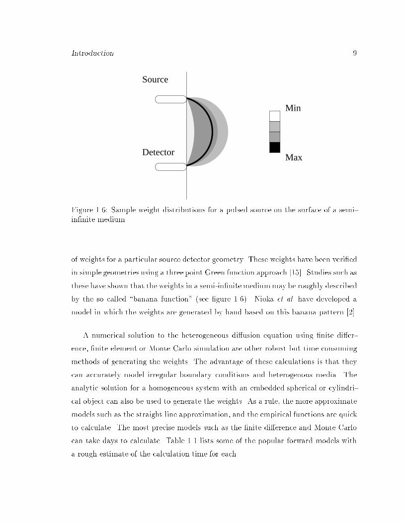
Figure 1.6: Sample weight distributions for a pulsed source on the surface of a semi-in�nite medium.
of weights for a particular source detector geometry. These weights have been veri�ed
in simple geometries using a three point Green function approach [15]. Studies such as
these have shown that the weights in a semi-in�nitemediummay be roughly described
by the so called \banana function" (see �gure 1.6). Nioka et al. have developed a
model in which the weights are generated by hand based on this banana pattern [2].
A numerical solution to the heterogeneous di�usion equation using �nite di�er-
ence, �nite element or Monte Carlo simulation are other robust but time consuming
methods of generating the weights. The advantage of these calculations is that they
can accurately model irregular boundary conditions and heterogenous media. The
analytic solution for a homogeneous system with an embedded spherical or cylindri-
cal object can also be used to generate the weights. As a rule, the more approximate
models such as the straight line approximation, and the empirical functions are quick
to calculate. The most precise models such as the �nite di�erence and Monte Carlo
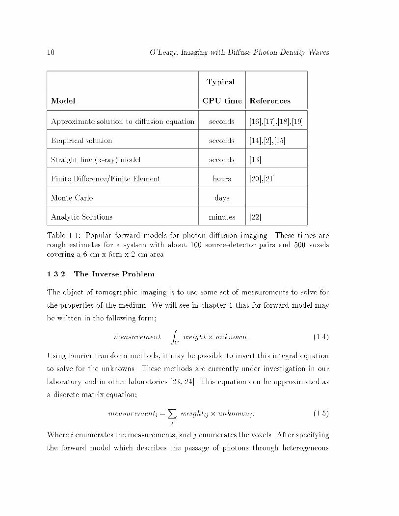
can take days to calculate. Table 1.1 lists some of the popular forward models with
a rough estimate of the calculation time for each.
10 O'Leary, Imaging with Di�use Photon Density Waves
Typical
Model CPU time References
Approximate solution to di�usion equation seconds [16],[17],[18],[19]
Empirical solution seconds [14],[2],[15]
Straight line (x-ray) model seconds [13]
Finite Di�erence/Finite Element hours [20],[21]
Monte Carlo days
Analytic Solutions minutes [22]
Table 1.1: Popular forward models for photon di�usion imaging. These times arerough estimates for a system with about 100 source-detector pairs and 500 voxels
covering a 6 cm x 6cm x 2 cm area.
1.3.2 The Inverse Problem
The object of tomographic imaging is to use some set of measurements to solve for
the properties of the medium. We will see in chapter 4 that for forward model may
be written in the following form;
measurement=ZV
weight� unknown: (1.4)
Using Fourier transform methods, it may be possible to invert this integral equation
to solve for the unknowns. These methods are currently under investigation in our
laboratory and in other laboratories [23, 24]. This equation can be approximated as
a discrete matrix equation;
measurementi =Xj
weightij � unknownj : (1.5)
Where i enumerates the measurements, and j enumerates the voxels. After specifying
the forward model which describes the passage of photons through heterogeneous
Introduction 11
media, the investigator must then invert the problem to solve for the unknown optical
properties in each voxel.
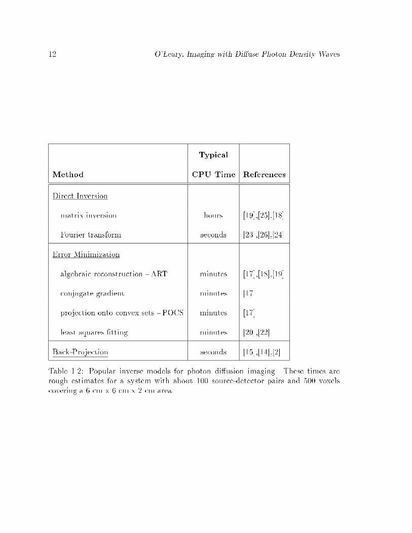
Table 1.2 lists some of the popular inversion methods. One set of methods is to
directly invert the forward equations to solve for the unknowns. Theoretically, the
direct matrix inversion should yield the unknowns in equation 1.5. But the inversion of
a large matrix is a time consuming calculation, and due to the nature of the problem,
the solutions are not unique. We will use regularization techniques to control the
uniqueness problem. In addition, the inverse matrix can be pre-calculated and stored
before the experiment.
There are many error minimization routines which �nd the unknowns by �tting the
forward model to the measured data. The error minimization routines mainly di�er
in the way that they move from an initial guess toward the correct solution. Some
error minimization methods, such as the algebraic reconstruction techniques (ART),
are only valid for linear equations. In our lab we use both ART and a direct matrix
inversion to create images. The relative merits of these techniques are discussed in
chapter 4.
Back-projection algorithms, often used in creating x-ray images, are gaining popu-
larity in photon imaging, especially for two dimensional projection images. Generally,
a back-projection algorithm will give a fast, rough image. In some cases we have used
a modi�ed back projection method which is brie y described in appendix D.
1.4 Resolution
The resolution of images with di�use photons is ultimately limited by the underlying
length scale of the di�usion theory, the random walk step of the photon (typically
about 1 mm in tissue). In our experiments, we have resolved two 1.2 cm diameter
spheres separated by a center-to-center distance of 2 cm. The resolution is depen-
dent on the wavelength of the DPDW. The shorter the wavelength, the better the
resolution. However, the positive e�ect of shortening the wavelength is o�set by the
fact that the amplitude of the wave decays exponentially at a spatial rate inversely
12 O'Leary, Imaging with Di�use Photon Density Waves
Typical
Method CPU Time References
Direct Inversion
matrix inversion hours [19],[25],[18]
Fourier transform seconds [23],[26],[24]
Error Minimization
algebraic reconstruction - ART minutes [17],[18],[19]
conjugate gradient minutes [17]
projection onto convex sets - POCS minutes [17]
least squares �tting minutes [20],[22]
Back-Projection seconds [15],[14],[2]
Table 1.2: Popular inverse models for photon di�usion imaging. These times are
rough estimates for a system with about 100 source-detector pairs and 500 voxelscovering a 6 cm x 6 cm x 2 cm area.
Introduction 13
proportional to the wavelength (ekr). The shorter the wavelength, the smaller the
measured signal. The wavelength can be shortened by increasing the modulation
frequency or increasing the background absorption or scattering.
Boas et al. have used a noise analysis to study the limits of object detection and
characterization [22]. The authors found that using a simulation based on realistic
positional uncertainties and shot noise, objects whose optical properties are approx-
imately twice the background levels and are 3 mm or larger can be detected and
localized; and objects 5 mm or larger can be characterized. The authors studied a
system designed to model a lightly compressed breast with an embedded tumor [27].
1.5 Contrast
Optical imaging provides fundamentally di�erent information than MRI, x-ray or
ultrasound imaging. Although we generate low resolution images, the contrasts are
optical properties, and this opens the door to a host of new physiologic mechanisms.
In our lab we have imaged absorption [28], the mean photon scattering length [18]
(reduced scattering coe�cient) and uorophore lifetimeand concentration [12]. In this
thesis, we will concentrate on these studies. Other work in our lab has demonstrated
imaging of the dynamic properties of scatterers, such as Brownian motion and ow
in model systems [29].
It important to note that by varying the incident optical wavelength it becomes
possible to perform spectroscopy in each of these contrasts. Researchers are just
beginning to investigate and quantify the optical changes which accompany physio-
logical changes in the body. There is considerable evidence that mitochondria are the
dominant light scatterers in most tissues [30]. This corroborates studies which show
that a rapidly growing tumor, which has an increased concentration of mitochondria,
is generally more highly scattering than the surrounding tissue [31]. A tumor also
has an increased vascularity, and thus a higher absorption due to the high volume
fraction of blood [31].
In the past two years, there has been a great deal of interest in the non-invasive
14 O'Leary, Imaging with Di�use Photon Density Waves
detection of glucose changes in the body [32, 15]. Since scattering depends on a mis-
match in the index of refraction, the presence of solutes such as glucose or potassium,
which change the index of refraction of the intra- or extra-cellular uid change the
scattering properties of the system.
In addition to natural optical changes, a wide range of optical dyes have been
developed for medical purposes. For example, the lifetime of some uorescent dyes
has been shown to vary with the amount of oxygen in its environment [33]. Some
dyes have already been approved by the FDA for other uses, but happen to be quite
useful for near infra-red imaging. Indocyanine green (ICG) has been used in liver
studies for over 20 years. Usually the dye is injected into the blood stream, and small
volumes of blood are taken every minute. The rapid decrease of ICG in the blood
indicates a that a healthy liver is removing the ICG.
It is possible that ICG will prove to be a useful contrast agent for optical tumor
detection. ICG has a strong absorption peak in the near infra-red (at 780 nm),
and uoresces at 830 nm making it an excellent candidate for optical studies. ICG's
molecular size is roughly the same as gadolinium chelate. Gadolinium chelate has been
shown to leak from the blood vessels in a rapidly growing tumor, and is currently
used as a MRI contrast agent for tumor detection.
The remainder of this thesis will follow the outline below. After a discussion of
di�use photon density waves (chapter 2), the experimental apparatus we use to mea-
sure the amplitude and phase of the waves will be discussed (chapter 3). Then we
move on to imaging. In chapter 4 we discuss the forward model and inverse algo-
rithms used to image inhomogeneous absorption. Computer simulated experiment
and experimental results are shown. Next we describe a parallel analysis for inho-
mogeneous scattering (chapter 5). Finally, we examine systems with both absorption
and scattering changes (chapter 6). In chapter 7 we discuss di�use photons in a
uorescent media. We develop the theory which describes uorescent di�use photon
density waves, show how these uorescent waves can be used to locate the center of
a uorescent object, and �nally we show that the lifetime and concentration of uo-
Introduction 15
rophore can be tomographically imaged in a manner similar to the absorption case.
Additional background information on singular matrices, time resolved spectroscopy
and the time-domain uorescent DPDW derivation is given in appendices A , B, and
C respectively. The results of some preliminary back-projection imaging work are
shown in appendix D. Appendix E gives an overview of the PMI software program
developed in our lab, and appendix F demonstrates a increase in PMI processing
speed using parallel processing.

16 O'Leary, Imaging with Di�use Photon Density Waves

Chapter 2
Optics for Di�use Photon Density Waves
In order to develop models for the forward and inverse problems, we must �rst under-
stand how photons travel through homogeneous media. In this section we begin by
describing the passage of photons through homogeneous media, and later incorporate
heterogeneous media using planar and curved boundaries. In this work we treat the
photons as particles, ignoring polarization and interference e�ects. This approach
is valid when the mean free path for photon scattering (1=�0
s) is much smaller than
the absorption length (1=�a) and much smaller than the sample size. The optical
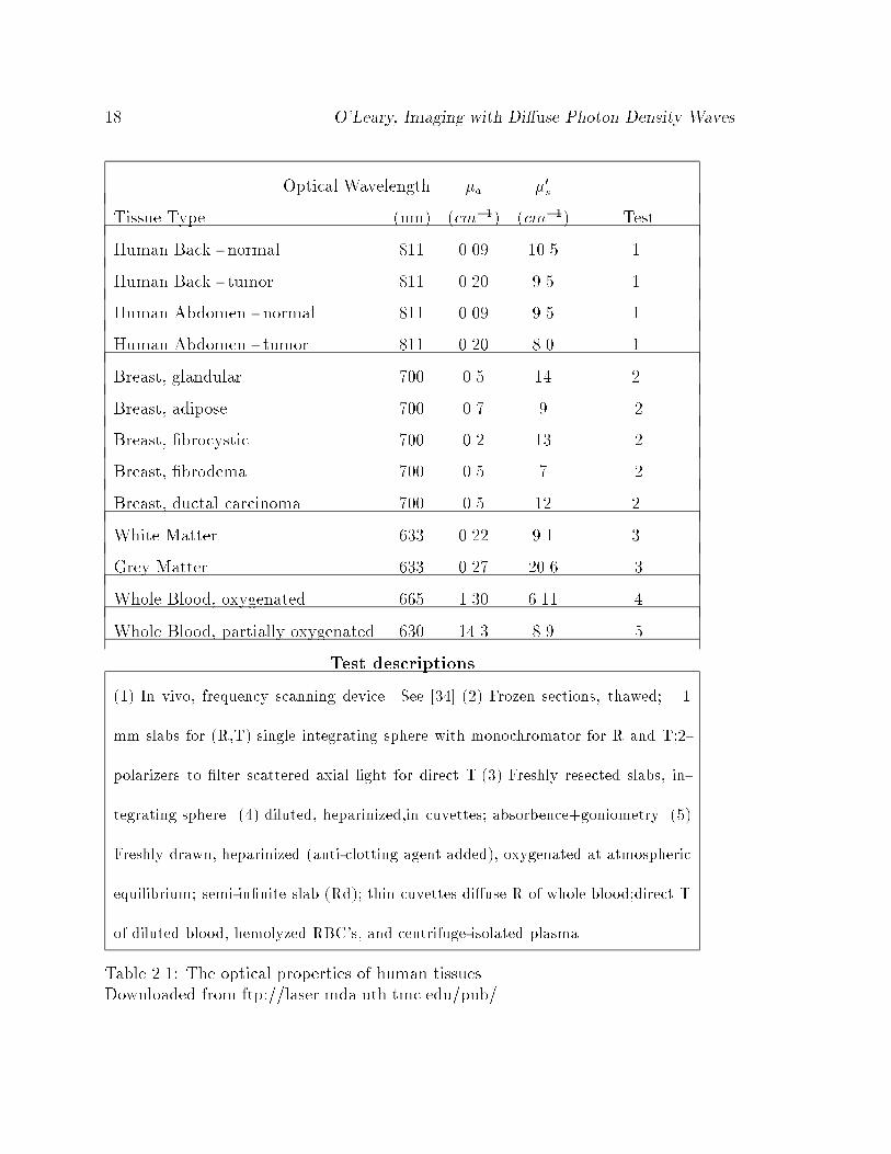
properties of some human tissues (table 2.1) demonstrate that this approximation is
good for systems such as the brain or breast, and source detector separations of a few
random walk steps.
As light enters such a medium, the photons undergo a random walk. When the
source-detector separation is much greater than the random walk mean free path, the
photon propagation can be modeled by the di�usion approximation to the Boltzmann
transport equation [3].
@U(r; t)
@t+ v�aU(r; t) +r � J(r; t) = qo(r; t); (2.1)
rU(r; t) +3@J(r; t)
v2@t+J(r; t)
D= 0 (2.2)
where U is the photon density (number of photons per unit volume), J is the photon
current density (number of photons per unit area per unit time), qo is the isotropic
source term (number of photons per unit volume per unit time), v is the speed of
17
18 O'Leary, Imaging with Di�use Photon Density Waves
Optical Wavelength �a �0
s
Tissue Type (nm) (cm�1) (cm�1) Test
Human Back - normal 811 0.09 10.5 1
Human Back - tumor 811 0.20 9.5 1
Human Abdomen - normal 811 0.09 9.5 1
Human Abdomen - tumor 811 0.20 8.0 1
Breast, glandular 700 0.5 14 2
Breast, adipose 700 0.7 9 2
Breast, �brocystic 700 0.2 13 2
Breast, �brodema 700 0.5 7 2
Breast, ductal carcinoma 700 0.5 12 2
White Matter 633 0.22 9.1 3
Grey Matter 633 0.27 20.6 3
Whole Blood, oxygenated 665 1.30 6.11 4
Whole Blood, partially oxygenated 630 14.3 8.9 5
Test descriptions
(1) In vivo, frequency scanning device. See [34] (2) Frozen sections, thawed; 1
mm slabs for (R,T) single integrating sphere with monochromator for R and T;2-
polarizers to �lter scattered axial light for direct T.(3) Freshly resected slabs, in-
tegrating sphere. (4) diluted, heparinized,in cuvettes; absorbence+goniometry. (5)
Freshly drawn, heparinized (anti-clotting agent added), oxygenated at atmospheric
equilibrium; semi-in�nite slab (Rd); thin cuvettes di�use R of whole blood;direct T
of diluted blood, hemolyzed RBC's, and centrifuge-isolated plasma.
Table 2.1: The optical properties of human tissues.Downloaded from ftp://laser.mda.uth.tmc.edu/pub/
Optics for DPDW's 19
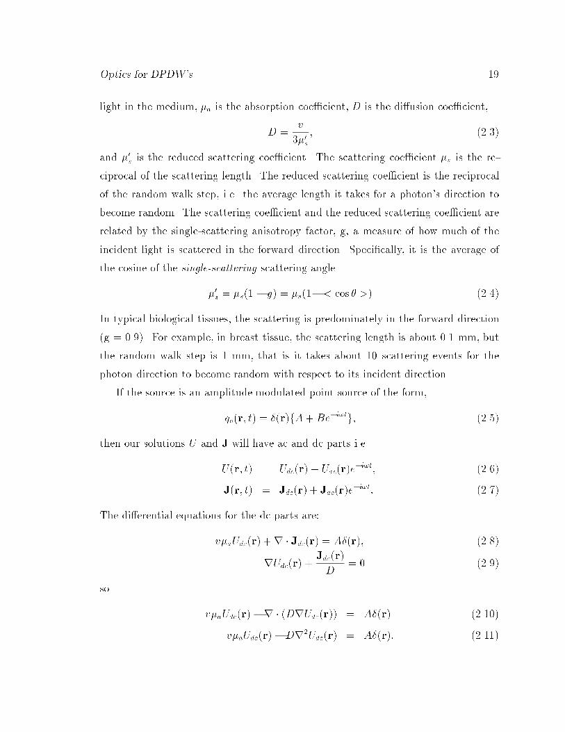
light in the medium, �a is the absorption coe�cient, D is the di�usion coe�cient,
D =v
3�0s
; (2.3)
and �0
s is the reduced scattering coe�cient. The scattering coe�cient �s is the re-
ciprocal of the scattering length. The reduced scattering coe�cient is the reciprocal
of the random walk step, i.e. the average length it takes for a photon's direction to
become random. The scattering coe�cient and the reduced scattering coe�cient are
related by the single-scattering anisotropy factor, g, a measure of how much of the
incident light is scattered in the forward direction. Speci�cally, it is the average of
the cosine of the single-scattering scattering angle.
�0
s = �s(1 � g) = �s(1� < cos � >) (2.4)
In typical biological tissues, the scattering is predominately in the forward direction
(g = 0.9). For example, in breast tissue, the scattering length is about 0.1 mm, but
the random walk step is 1 mm, that is it takes about 10 scattering events for the
photon direction to become random with respect to its incident direction.
If the source is an amplitude modulated point source of the form,
qo(r; t) = �(r)fA+Be�i!tg; (2.5)
then our solutions U and J will have ac and dc parts i.e.
U(r; t) = Udc(r) + Uac(r)e�i!t; (2.6)
J(r; t) = Jdc(r) + Jac(r)e�i!t: (2.7)
The di�erential equations for the dc parts are:
v�aUdc(r) +r � Jdc(r) = A�(r); (2.8)
rUdc(r) +Jdc(r)
D= 0 (2.9)
so
v�aUdc(r)�r � (DrUdc(r)) = A�(r) (2.10)
v�aUdc(r)�Dr2Udc(r) = A�(r): (2.11)
20 O'Leary, Imaging with Di�use Photon Density Waves
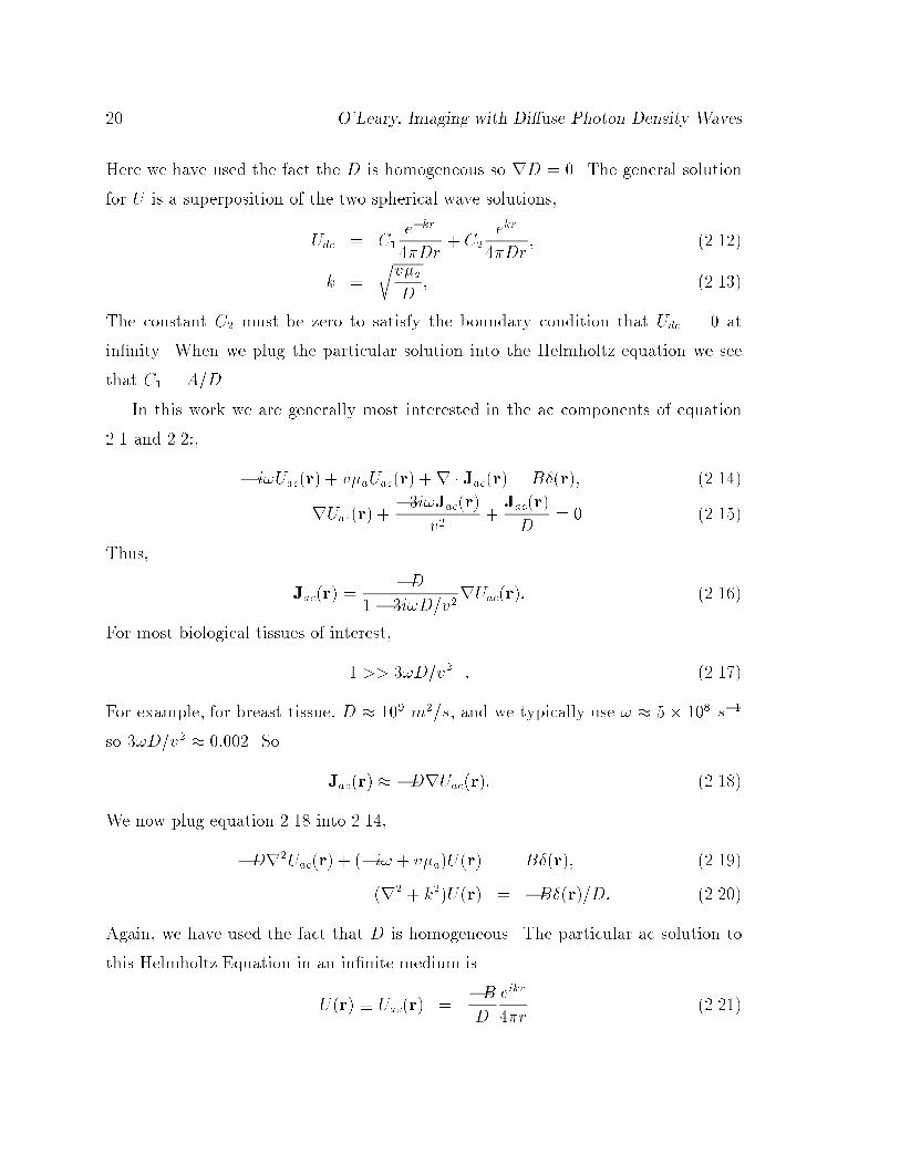
Here we have used the fact the D is homogeneous so rD = 0. The general solution
for U is a superposition of the two spherical wave solutions,
Udc = C1
e�kr
4�Dr+ C2
ekr
4�Dr; (2.12)
k =
rv�a
D; (2.13)
The constant C2 must be zero to satisfy the boundary condition that Udc = 0 at
in�nity. When we plug the particular solution into the Helmholtz equation we see
that C1 = A=D.
In this work we are generally most interested in the ac components of equation
2.1 and 2.2:,
� i!Uac(r) + v�aUac(r) +r � Jac(r) = B�(r); (2.14)
rUac(r) +�3i!Jac(r)
v2+Jac(r)
D= 0 (2.15)
Thus,
Jac(r) =�D
1� 3i!D=v2rUac(r): (2.16)
For most biological tissues of interest,
1 >> 3!D=v2 : (2.17)
For example, for breast tissue, D � 109 m2=s, and we typically use ! � 5 � 108 s�1
so 3!D=v2 � 0:002. So
Jac(r) � �DrUac(r): (2.18)
We now plug equation 2.18 into 2.14,
�Dr2Uac(r) + (�i! + v�a)U(r) = B�(r); (2.19)
(r2 + k2)U(r) = �B�(r)=D: (2.20)
Again, we have used the fact that D is homogeneous. The particular ac solution to
this Helmholtz Equation in an in�nite medium is
U(r) � Uac(r) =�B
D
eikr
4�r(2.21)
Optics for DPDW's 21
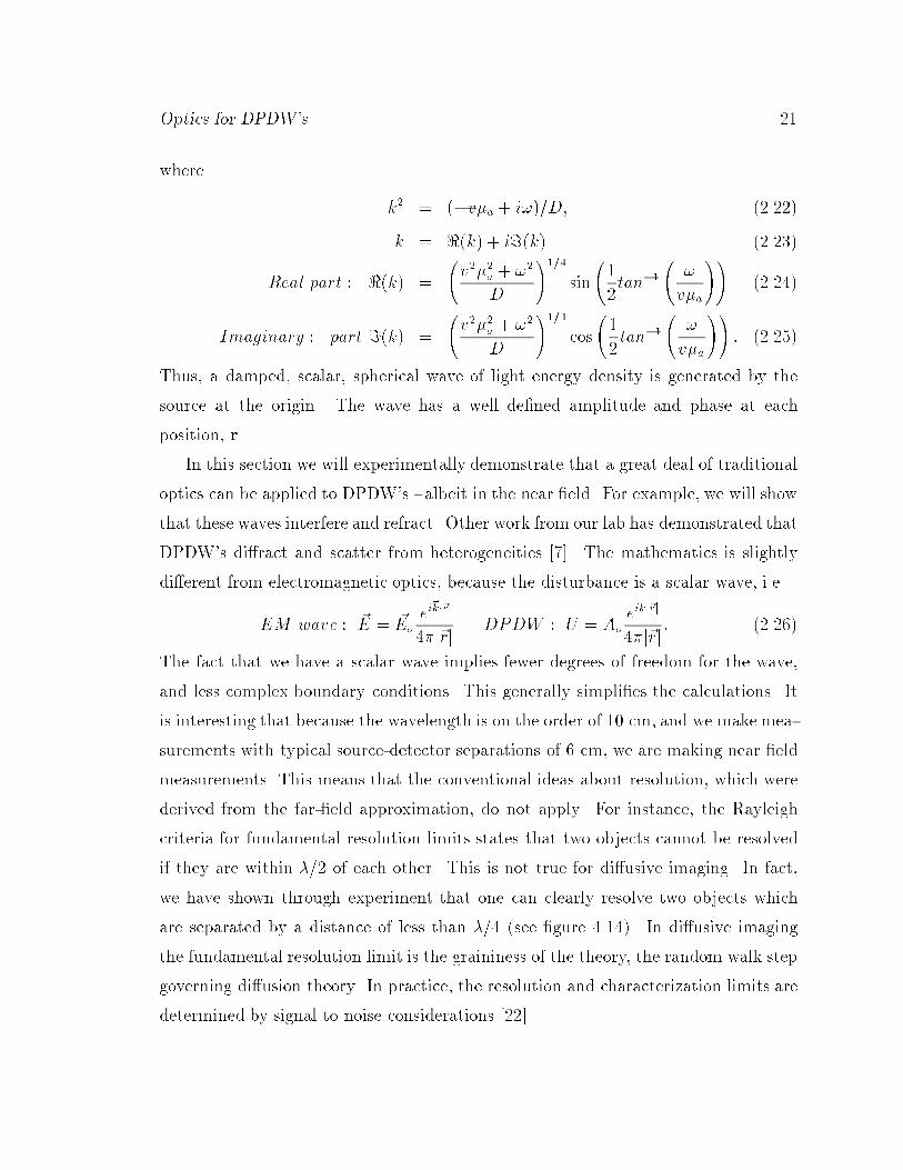
where
k2 = (�v�a + i!)=D; (2.22)
k = <(k) + i=(k) (2.23)
Real part : <(k) =
v2�2a + !2
D
!1=4
sin
1
2tan�1
!
v�a
!!(2.24)
Imaginary : part =(k) =
v2�2a + !2
D
!1=4
cos
1
2tan�1
!
v�a
!!: (2.25)
Thus, a damped, scalar, spherical wave of light energy density is generated by the
source at the origin. The wave has a well de�ned amplitude and phase at each
position, r.
In this section we will experimentally demonstrate that a great deal of traditional
optics can be applied to DPDW's - albeit in the near �eld. For example, we will show
that these waves interfere and refract. Other work from our lab has demonstrated that
DPDW's di�ract and scatter from heterogeneities [7]. The mathematics is slightly
di�erent from electromagnetic optics, because the disturbance is a scalar wave, i.e.
EM wave : ~E = ~Eo
ei~k�~r
4�j~rjDPDW : U = Ao
eikj~rj
4�j~rj: (2.26)
The fact that we have a scalar wave implies fewer degrees of freedom for the wave,
and less complex boundary conditions. This generally simpli�es the calculations. It
is interesting that because the wavelength is on the order of 10 cm, and we make mea-
surements with typical source-detector separations of 6 cm, we are making near �eld
measurements. This means that the conventional ideas about resolution, which were
derived from the far-�eld approximation, do not apply. For instance, the Rayleigh
criteria for fundamental resolution limits states that two objects cannot be resolved
if they are within �=2 of each other. This is not true for di�usive imaging. In fact,
we have shown through experiment that one can clearly resolve two objects which
are separated by a distance of less than �=4 (see �gure 4.14). In di�usive imaging
the fundamental resolution limit is the graininess of the theory, the random walk step
governing di�usion theory. In practice, the resolution and characterization limits are
determined by signal to noise considerations [22].
22 O'Leary, Imaging with Di�use Photon Density Waves
We begin by demonstrating that these waves exist in a homogeneous, in�nite
medium. Our experimental setup consisted of a large �sh tank (30 x 30 x 60 cm)
�lled with a model biological material called Intralipid [35]. Intralipid is a turbid,
polydisperse suspension of soy lipid. The particle diameter ranges from about 0.1�m
to 1.1�m with an average of about 0.4�m. By changing the solution concentration
one can vary the light di�usion constant over a wide range. We typically use con-
centrations varying from 0.1% (D = 7:5 � 109m2=s) to 1.5% (D = 5:0 � 109m2=s).
We can also add inks (such as india ink) and dyes (such as any water soluble laser
dye) to vary the absorption coe�cient. The absorption of the inks and dyes can be
calibrated in a standard spectrophotometer. A laser diode was �ber coupled to the
medium using a 0.3 cm diameter �ber bundle, and a similar optical �ber was used to
detect di�use photons. A translation stage enabled measurements of amplitude and
phase as a function of position within the tank.
The experimental setup is described in detail in chapter 3. Brie y, source and
detector optical �bers (�3 mm in diameter) were immersed in the solution at the
same height above the tank oor (see �gure 2.1). The source light was derived from
a 3 mW diode laser operating at 780 nm. The diode laser was amplitude modulated
at 200 MHz. The detector �ber could be positioned anywhere in the plane, and
was connected to a photomultiplier tube on its other end. In order to facilitate the
phase and amplitude measurements, both the reference signal from the source and
the detected signal were down-converted to 25 kHz by heterodyning with a second
oscillator at 200.025 MHz. The low frequency signals were then measured using
a lock-in ampli�er. The phase shift and AC amplitude of the detected light were
measured with respect to the source at each point on a 0.5 cm square planar grid
throughout the sample. Constant phase contours were easily determined by linear
interpolation of the grid data. Since the signal amplitude decays by a factor of e2�=r
in one wavelength, the range of our experiments is limited to slightly more than one
wavelength. Nevertheless it is possible to clearly distinguish the essential physical
phenomena in the experiments.
Optics for DPDW's 23
Throughout this work, we assume that we have an isotropic point source and a
point detector. In reality, we have a �nite detector area (usually about 3 mm diame-
ter) and a nearly collimated source �ber with a �nite size (usually 1-3 mm diameter).
In a collimnated source, the light will travel ballistically for approximately one ran-
dom walk step. After 1 random walk step, a signi�cant portion of the light has been
scattered, and the isotropic source approximation is a good approximation. Some
researchers place an e�ective source one random walk step away from the true source
to correct for this e�ect. In this work we have not investigated or used a correction
method. This will contribute small errors in the experimental measurements.
Figure 2.1 shows the measured constant phase contours of the disturbance pro-
duced by a �ber source located at the origin. First we note that the phase contours
are spherical and centered about the source position. Second, both the phase and
the log of the amplitude times the source-detector separation are linear with the
source-detection separation as shown in the inset of �gure 2.1. We can calculate the
absorption and scattering coe�cients of the medium from the measurements of am-
plitude and phase. Typically, we characterize a medium by measuring the amplitude
and phase as a function of distance. The slopes of these lines give us the real and
imaginary parts of the wavenumber k;
ln(rjU(r)j) = �=(k)r + ln(B)� ln(4�D) ; (2.27)
phase(U(r)) = <(k)r : (2.28)
Once we know k, we can easily calculate the absorption and and reduced scattering
of the medium,
1=�a =v
!tan
2 tan�1
<(k)
=(k)
!!(2.29)
1=D =<(k)2 + =(k)2
(v2�2a + !2)1=2: (2.30)
From these measurements we deduced the wavelength of the di�use photon density
wave (11.2 cm), as well as the photon transport mean free path (0.1 cm), and the

24 O'Leary, Imaging with Di�use Photon Density Waves
0.5% Intralipid
Source Detector
Translation Stage
Optical Fiber
Position (cm)
Pos
ition
(cm
)
ln |rA
C |
Distance (cm)
Pha
se (
degr
ees)
Figure 2.1: Constant phase contours shown as a function of position for homogeneous,0.5% Intralipid solution. The contours are shown in 20 degree intervals. Inset: Themeasured phase shift (circles), and ln(rUac(r)) (squares) are plotted as a function ofradial distance from the source So.
Optics for DPDW's 25
photon absorption length (52.4 cm) in 0.5% Intralipid at room temperature. The
photon absorption can be attributed almost entirely to water [36] at 780 nm.
In �gure 2.2 we demonstrate the refraction of these waves in three ways. Figure
2.2 shows constant phase contours (every 20� ). This time however, a plane boundary
was introduced, separating the lower medium with concentration [l] = 1.0% and light
di�usion coe�cient Dl, from the upper medium with concentration [u] = 0.25% and
light di�usion coe�cient Du. The contours below the boundary are just the homo-
geneous media contours (without re ection); they were obtained before the partition
was introduced into the sample. The contours above the boundary were derived from
the di�use photon density waves transmitted into the less concentrated medium. As
a result of our detector geometry, our closest approach to the partition was about 1
cm. We expect a number of general results. First, the wavelength in the less dense
medium ( �u = 14.8 cm ) should be greater than the wavelength of the di�use photon
density wave in the incident medium ( �l = 8.17 cm ). This was observed. The ratio
of the two wavelengths should equal the ratio of the di�usive indices of refraction of
the two media. Speci�cally we found, as expected, that
�u = �l
sDl
Du
� �l
vuut [l]
[u]: (2.31)
We would expect that the apparent source position (Si), as viewed from within the
upper medium, should be shifted from the real source position (So = 4.0 � 0.2 cm)
by the factor �l / �u = 0.55. Using the the radii from the full contour plots, we see
that the apparent source position is shifted from 4.0 � 0.2 cm to 2.0 � 0.25 cm.
Finally in �gure 2.2 we explicitly demonstrate Snell's law for di�use photon density
waves. This can be seen by following the ray from So to the point A at the boundary,
and then into the upper medium. The ray in the lower medium makes an angle �i =
14� with respect to the surface normal. The upper ray is constructed in the standard
way between the apparent source position Si, through the point A on the boundary,
and into the medium above the boundary [37]. It is perpendicular to the circular
wavefronts in the less dense medium, and makes an angle �t = 26.6� with respect to
26 O'Leary, Imaging with Di�use Photon Density Waves
the boundary normal. Within the accuracy of the experiment we see that
sin(�i)
sin(�t)= 0:54 �
�l
�u; (2.32)
Thus Snell's law accurately describes the propagation of di�use photon density waves
across the boundary. It is interesting to note that the wavefronts become quite dis-
torted when the source ray angle exceeds 30� . These irregularities are a consequence
of total internal re ection, di�raction, and some spurious boundary e�ects.
A third important observation is presented in �gure 2.3. We used a circular
boundary separating two turbid media to demonstrate that we can alter the curvature
of the di�use photon density wavefronts in analogy with a simple lens in optics. The
constant phase contours on the left occur in 20� intervals, and the constant phase
contours on the right occur in 40� intervals. The constant phase contours of the
transmitted wave exhibit a shorter wavelength, and are clearly converging toward
some image point to the right of the boundary. The medium on the left (ll) has
an Intralipid concentration of [l] � 0.1%, and the medium on the right (lr) has a
concentration of [r] � 1.6%. The wavelength ratio was measured to be lr=ll = 3.8 �
0.3. The curved surface has a radius R = 9.0 � 0.4 cm. The object position (the
source) is So = 9.4 � 0.3 cm, and the image position Si = 10:9 cm is predicted from
the well known paraxial result from geometrical optics for imaging by a spherical
refracting surface [37];q1=[l]
So
+
q1=[r]
Si
=
q1=[r] �
q1=[l]
R(2.33)
The image position was measured to be Si = 12 � 2 cm, which is close to the predicted
value, 10.9 cm. The image position was found by using a compass to determine
the center of the four wavefronts. Although the error in this measurement is large,
the central point remains, that is, the curvature of the wavefronts is reversed after
traversing the circular boundary.
DPDW's have also been shown to interfere. In much of our work, we will exploit
the destructive interference of two DPDW's to increase our sensitivity to hetero-
geneities [9] and reduce our sensitivity to the background properties. In a typical
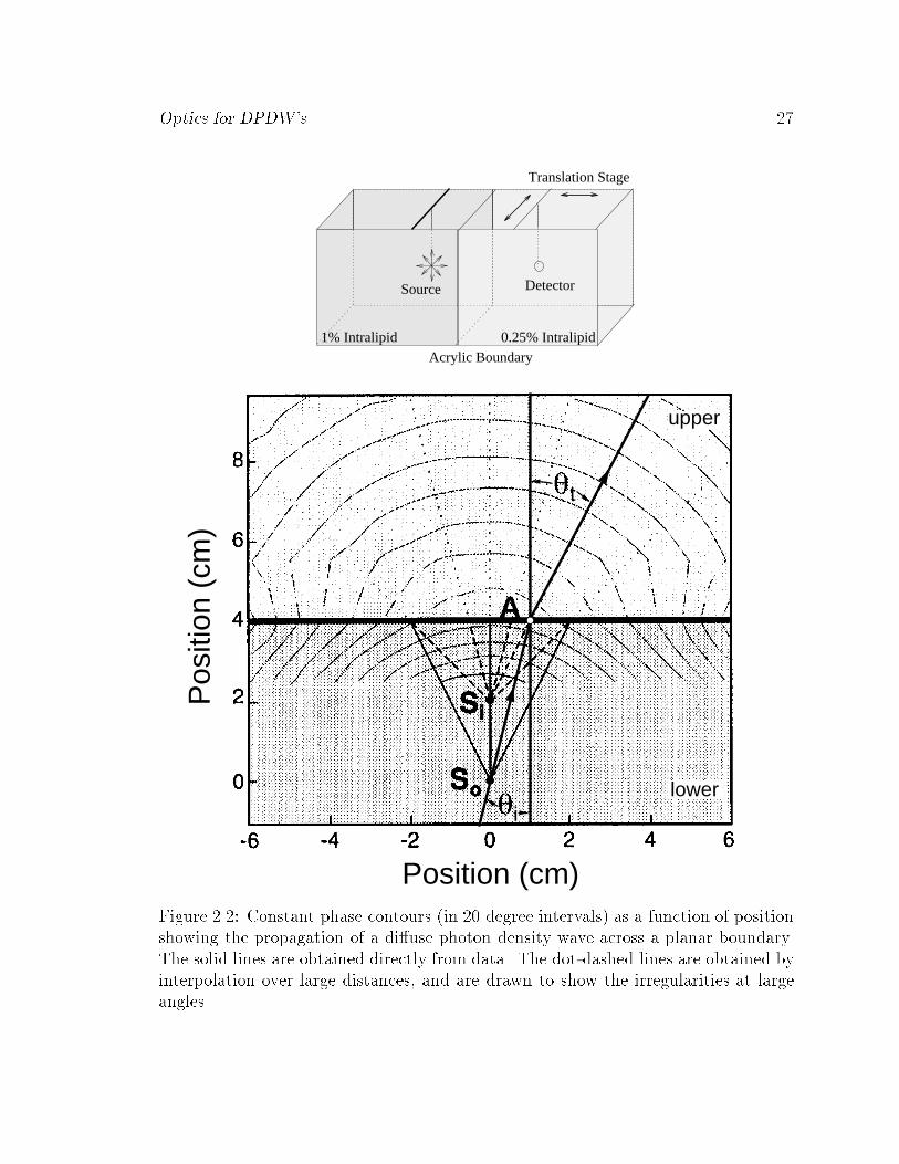
Optics for DPDW's 27
Translation Stage
1% Intralipid 0.25% Intralipid
Source Detector
Acrylic Boundary
A
t
i
Position (cm)
Pos
ition
(cm
)
upper
lower
Figure 2.2: Constant phase contours (in 20 degree intervals) as a function of positionshowing the propagation of a di�use photon density wave across a planar boundary.The solid lines are obtained directly from data. The dot-dashed lines are obtained byinterpolation over large distances, and are drawn to show the irregularities at largeangles.
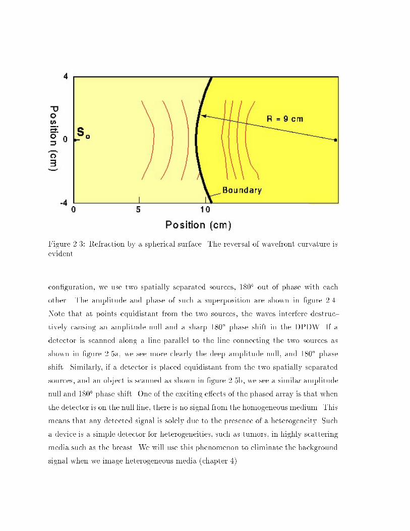
28 O'Leary, Imaging with Di�use Photon Density Waves
Figure 2.3: Refraction by a spherical surface. The reversal of wavefront curvature isevident.
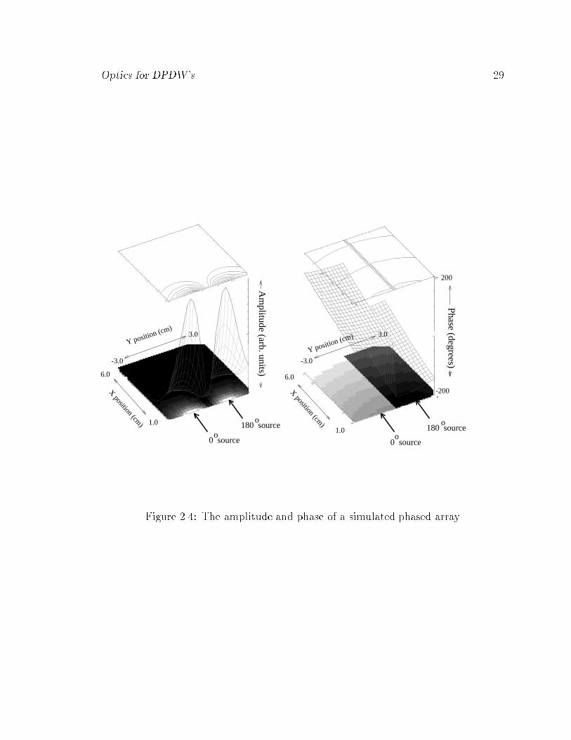
con�guration, we use two spatially separated sources, 180� out of phase with each
other. The amplitude and phase of such a superposition are shown in �gure 2.4.
Note that at points equidistant from the two sources, the waves interfere destruc-
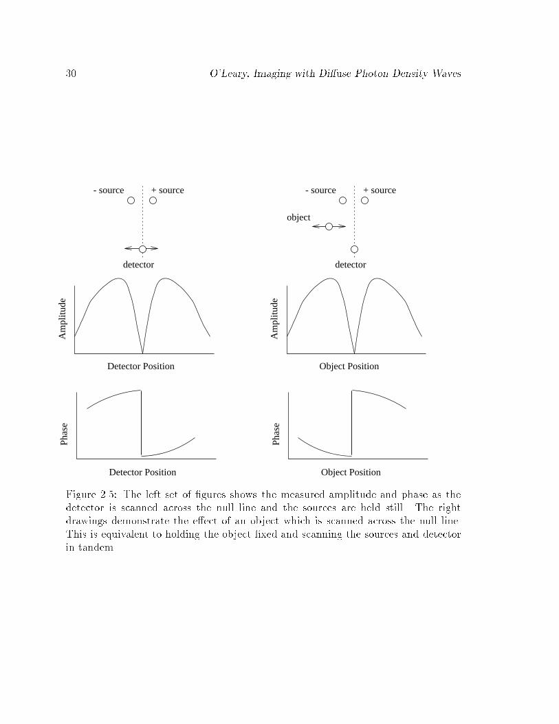
tively causing an amplitude null and a sharp 180� phase shift in the DPDW. If a
detector is scanned along a line parallel to the line connecting the two sources as
shown in �gure 2.5a, we see more clearly the deep amplitude null, and 180� phase
shift. Similarly, if a detector is placed equidistant from the two spatially separated
sources, and an object is scanned as shown in �gure 2.5b, we see a similar amplitude
null and 180� phase shift. One of the exciting e�ects of the phased array is that when
the detector is on the null line, there is no signal from the homogeneous medium. This
means that any detected signal is solely due to the presence of a heterogeneity. Such
a device is a simple detector for heterogeneities, such as tumors, in highly scattering
media such as the breast. We will use this phenomenon to eliminate the background
signal when we image heterogeneous media (chapter 4).
Optics for DPDW's 29
Phase (degrees)
3.0
-3.0
3.0
-3.0
0 sourceo o
0 source
6.0
1.0180 source
o
6.0
-200
200
X position (cm) 1.0
X position (cm)
Y position (cm)
Y position (cm)
180 sourceo
Am
plitude (arb. units)
Figure 2.4: The amplitude and phase of a simulated phased array
30 O'Leary, Imaging with Di�use Photon Density Waves
+ source- source
detectorPh
ase
Am
plitu
de
object
+ source- source
detector
Detector Position
Phas
eA
mpl
itude
Detector Position Object Position
Object Position
Figure 2.5: The left set of �gures shows the measured amplitude and phase as thedetector is scanned across the null line and the sources are held still. The rightdrawings demonstrate the e�ect of an object which is scanned across the null line.This is equivalent to holding the object �xed and scanning the sources and detectorin tandem.
Optics for DPDW's 31
simultaneous measurement
2 source
(c)
2 detector
subtracted simultaneous measurement
2 single source measuments
(b)
detector detector
source source
(a)
-
sourcedetector
+ source - source + detector - detector
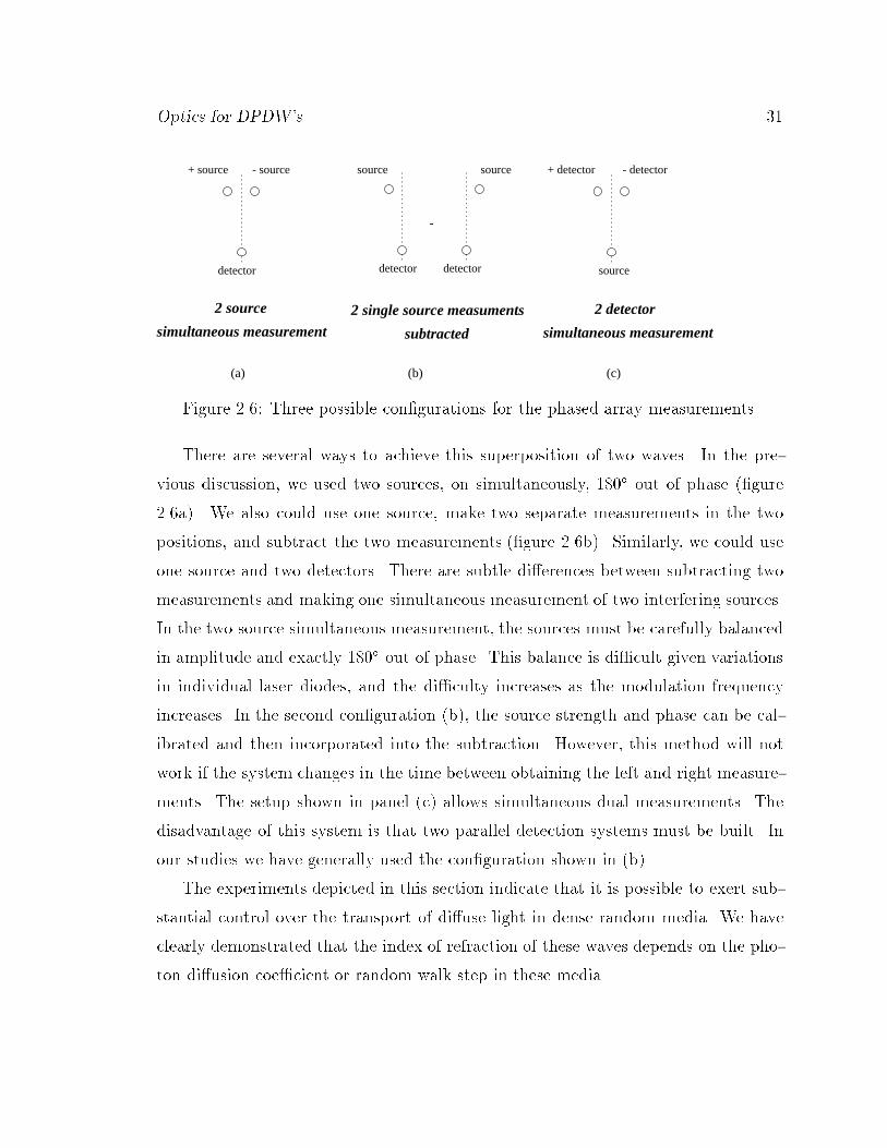
Figure 2.6: Three possible con�gurations for the phased array measurements.
There are several ways to achieve this superposition of two waves. In the pre-
vious discussion, we used two sources, on simultaneously, 180� out of phase (�gure
2.6a). We also could use one source, make two separate measurements in the two
positions, and subtract the two measurements (�gure 2.6b). Similarly, we could use
one source and two detectors. There are subtle di�erences between subtracting two
measurements and making one simultaneous measurement of two interfering sources.
In the two source simultaneous measurement, the sources must be carefully balanced
in amplitude and exactly 180� out of phase. This balance is di�cult given variations
in individual laser diodes, and the di�culty increases as the modulation frequency
increases. In the second con�guration (b), the source strength and phase can be cal-
ibrated and then incorporated into the subtraction. However, this method will not
work if the system changes in the time between obtaining the left and right measure-
ments. The setup shown in panel (c) allows simultaneous dual measurements. The
disadvantage of this system is that two parallel detection systems must be built. In
our studies we have generally used the con�guration shown in (b).
The experiments depicted in this section indicate that it is possible to exert sub-
stantial control over the transport of di�use light in dense random media. We have
clearly demonstrated that the index of refraction of these waves depends on the pho-
ton di�usion coe�cient or random walk step in these media.
32 O'Leary, Imaging with Di�use Photon Density Waves
Chapter 3
Hardware Speci�cations
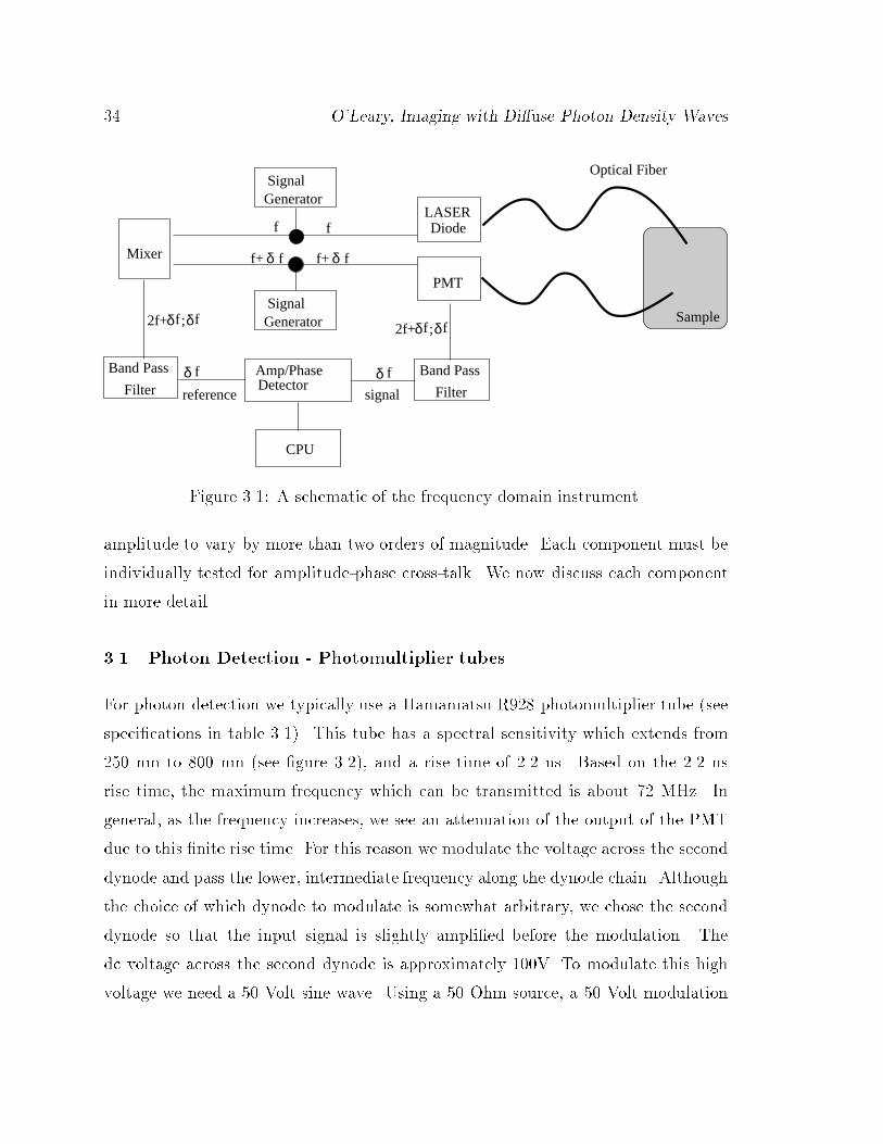
A schematic of the phase modulation device is shown in �gure 3.1. The driving current
of a laser diode is modulated at a high (radio) frequency, ! = 2�f , causing the output
of the diode to be intensity modulated. The modulated light passes through the
sample medium, and the intensity is monitored using a photomultiplier tube (PMT).
A second radio frequency source with an angular frequency of !+ �! = 2�(f + �f) is
used to modulate the gain of the detector. 3 mm diameter multimode �ber bundles
deliver the modulated light from the laser source to the medium, and from the medium
to the PMT.
The current output of the PMT is proportional to the modulated intensity and
the modulated gain (as described in more detail below). By modulating the gain, a
\mixed" current composed of sum and di�erence frequencies is generated. The sum
and di�erence frequency signals are passed through a band pass �lter centered around
the di�erence frequency, �!. A reference signal is generated in a similar manner by
electronically mixing a portion of the two RF signals and then passing the output
reference signal through a similar band pass �lter centered at �!. The phase and
amplitude of the DPDW are measured with respect to the reference signal using
traditional lock-in techniques. In our system we typically use a frequency of around
f = 200 MHz, and an intermediate frequency of �f = 26:6 KHz.
A great deal of care must be taken when measuring the phase shift. Many elec-
tronic devices will measure phase accurately as long as the amplitude of the signal is
approximately constant. Since we have an exponentially damped signal, we expect to
33
34 O'Leary, Imaging with Di�use Photon Density Waves
Mixer
PMT
Filter
Band PassFilter
Band Pass
Optical Fiber
signalreference
LASERDiode
Sample
f f
; fδfδ2f+
δ f
ff+ δ ff+ δ
;2f+ fδ fδ
δ fAmp/Phase Detector
CPU
GeneratorSignal
GeneratorSignal
Figure 3.1: A schematic of the frequency domain instrument.
amplitude to vary by more than two orders of magnitude. Each component must be
individually tested for amplitude-phase cross-talk. We now discuss each component
in more detail.
3.1 Photon Detection - Photomultiplier tubes
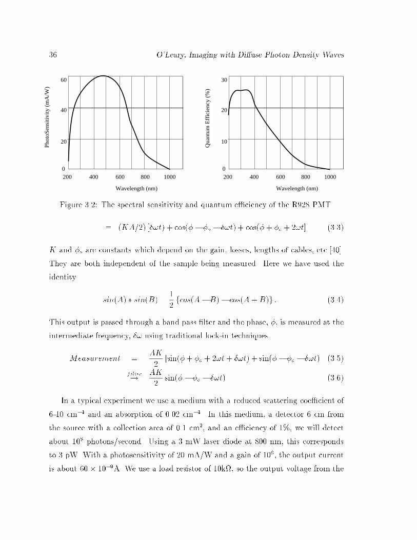
For photon detection we typically use a Hamamatsu R928 photomultiplier tube (see
speci�cations in table 3.1). This tube has a spectral sensitivity which extends from
250 nm to 800 nm (see �gure 3.2), and a rise time of 2.2 ns. Based on the 2.2 ns
rise time, the maximum frequency which can be transmitted is about 72 MHz. In
general, as the frequency increases, we see an attenuation of the output of the PMT
due to this �nite rise time. For this reason we modulate the voltage across the second
dynode and pass the lower, intermediate frequency along the dynode chain. Although
the choice of which dynode to modulate is somewhat arbitrary, we chose the second
dynode so that the input signal is slightly ampli�ed before the modulation. The
dc voltage across the second dynode is approximately 100V. To modulate this high
voltage we need a 50 Volt sine wave. Using a 50 Ohm source, a 50 Volt modulation
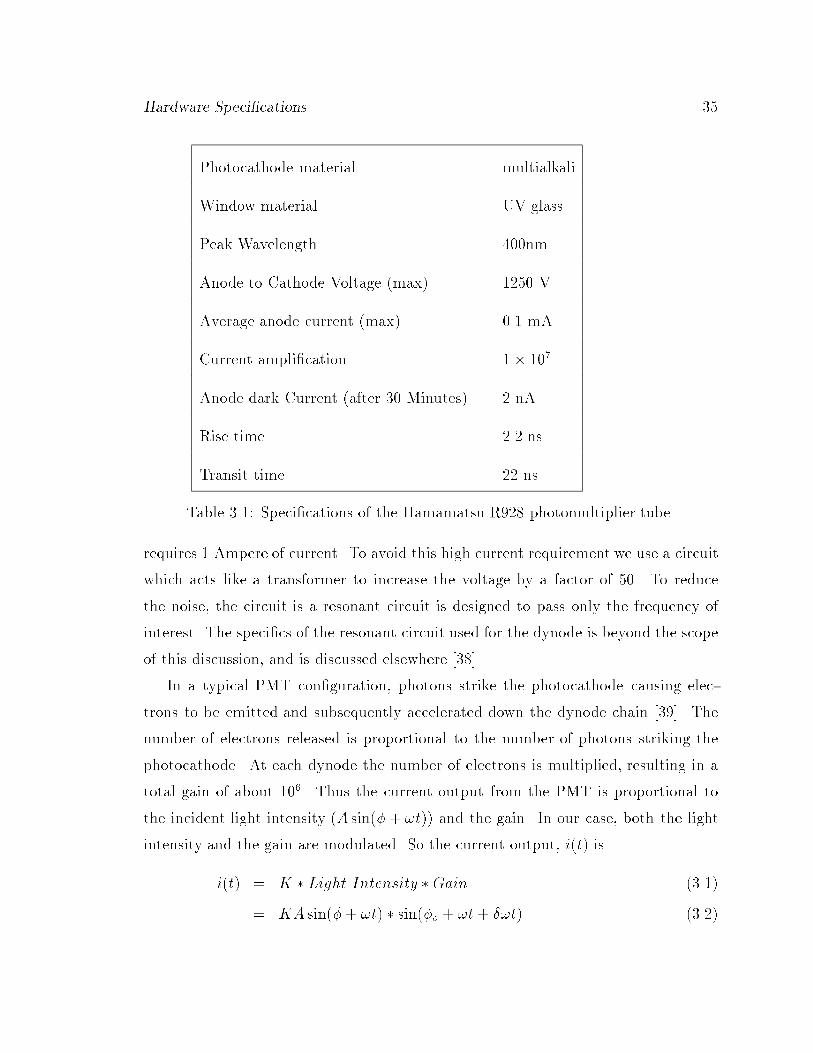
Hardware Speci�cations 35
Photocathode material multialkali
Window material UV glass
Peak Wavelength 400nm
Anode to Cathode Voltage (max) 1250 V
Average anode current (max) 0.1 mA
Current ampli�cation 1� 107
Anode dark Current (after 30 Minutes) 2 nA
Rise time 2.2 ns
Transit time 22 ns
Table 3.1: Speci�cations of the Hamamatsu R928 photomultiplier tube.
requires 1 Ampere of current. To avoid this high current requirement we use a circuit
which acts like a transformer to increase the voltage by a factor of 50. To reduce
the noise, the circuit is a resonant circuit is designed to pass only the frequency of
interest. The speci�cs of the resonant circuit used for the dynode is beyond the scope
of this discussion, and is discussed elsewhere [38].
In a typical PMT con�guration, photons strike the photocathode causing elec-
trons to be emitted and subsequently accelerated down the dynode chain [39]. The
number of electrons released is proportional to the number of photons striking the
photocathode. At each dynode the number of electrons is multiplied, resulting in a
total gain of about 106. Thus the current output from the PMT is proportional to
the incident light intensity (A sin(� + !t)) and the gain. In our case, both the light
intensity and the gain are modulated. So the current output, i(t) is
i(t) = K � Light Intensity �Gain (3.1)
= KA sin(�+ !t) � sin(�o + !t+ �!t) (3.2)
36 O'Leary, Imaging with Di�use Photon Density Waves
200 400 600 800 1000
Wavelength (nm)
0
60
40
20
Phot
oSen
sitiv
ity (
mA
/W)
200 400 600 800 1000
Wavelength (nm)
0
30
20
10
Qua
ntum
Eff
icie
ncy
(%)
Figure 3.2: The spectral sensitivity and quantum e�ciency of the R928 PMT.
= (KA=2) [�!t) + cos(�� �o � �!t) + cos(�+ �o + 2!t] (3.3)
K and �o are constants which depend on the gain, losses, lengths of cables, etc.[40].
They are both independent of the sample being measured. Here we have used the
identity
sin(A) � sin(B) =1
2fcos(A�B)� cos(A+B)g : (3.4)
This output is passed through a band pass �lter and the phase, �, is measured at the
intermediate frequency, �! using traditional lock-in techniques.
Measurement =AK
2[sin(�+ �o + 2!t+ �!t) + sin(�� �o � �!t)] (3.5)
filter!
AK
2sin(�� �o � �!t) (3.6)
In a typical experiment we use a medium with a reduced scattering coe�cient of
6-10 cm�1 and an absorption of 0.02 cm�1. In this medium, a detector 6 cm from
the source with a collection area of 0.1 cm2, and an e�ciency of 1%, we will detect
about 108 photons/second. Using a 3 mW laser diode at 800 nm, this corresponds
to 3 pW. With a photosensitivity of 20 mA/W and a gain of 106, the output current
is about 60 � 10�9A. We use a load resistor of 10k, so the output voltage from the
Hardware Speci�cations 37
Mixer
GeneratorFunction
GeneratorFunction
PMT
Filter
Density
Filters
Neutral
Optical Fiber
signalreference
LASERDiode
FilterAmp/Phase Detector
CPU
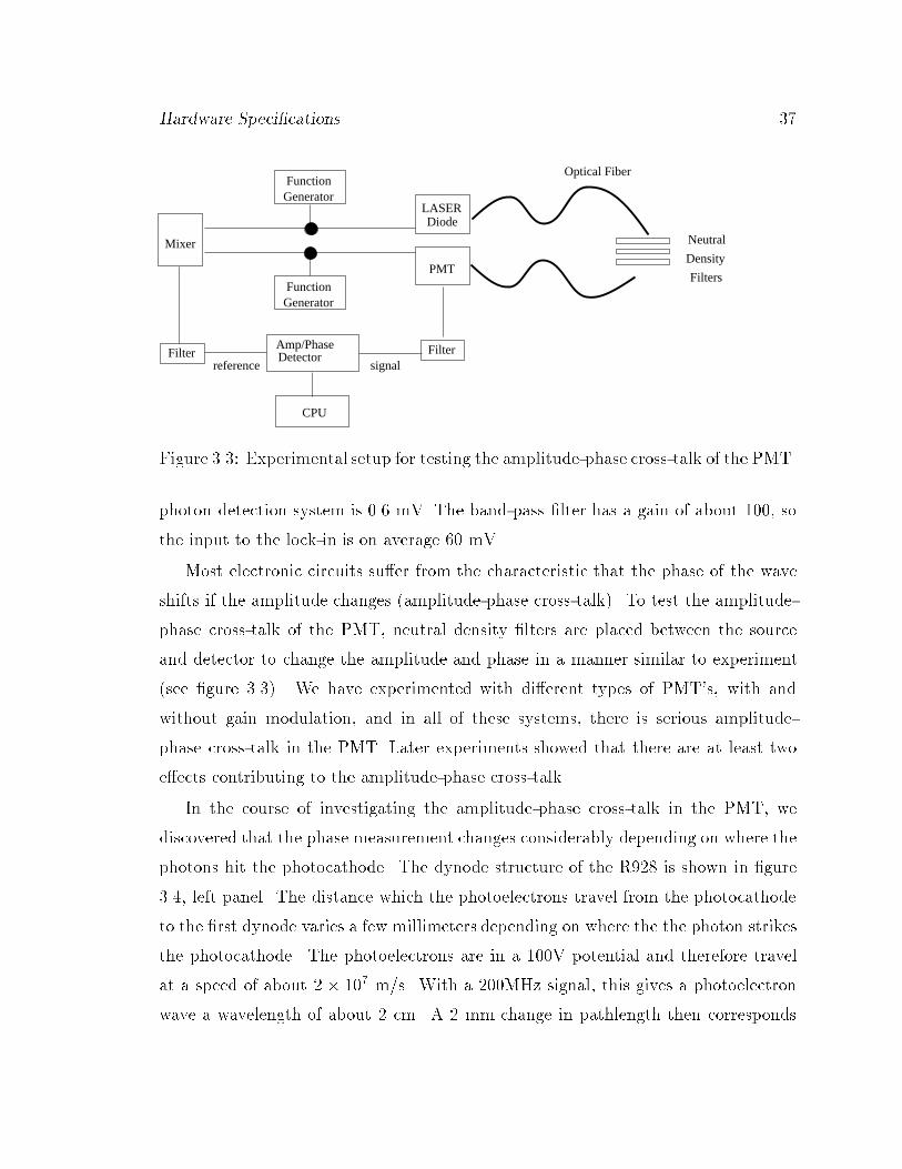
Figure 3.3: Experimental setup for testing the amplitude-phase cross-talk of the PMT.
photon detection system is 0.6 mV. The band-pass �lter has a gain of about 100, so
the input to the lock-in is on average 60 mV.
Most electronic circuits su�er from the characteristic that the phase of the wave
shifts if the amplitude changes (amplitude-phase cross-talk). To test the amplitude-
phase cross-talk of the PMT, neutral density �lters are placed between the source
and detector to change the amplitude and phase in a manner similar to experiment
(see �gure 3.3). We have experimented with di�erent types of PMT's, with and
without gain modulation, and in all of these systems, there is serious amplitude-
phase cross-talk in the PMT. Later experiments showed that there are at least two
e�ects contributing to the amplitude-phase cross-talk.
In the course of investigating the amplitude-phase cross-talk in the PMT, we
discovered that the phase measurement changes considerably depending on where the
photons hit the photocathode. The dynode structure of the R928 is shown in �gure
3.4, left panel. The distance which the photoelectrons travel from the photocathode
to the �rst dynode varies a few millimeters depending on where the the photon strikes
the photocathode. The photoelectrons are in a 100V potential and therefore travel
at a speed of about 2 � 107 m/s. With a 200MHz signal, this gives a photoelectron
wave a wavelength of about 2 cm. A 2 mm change in pathlength then corresponds
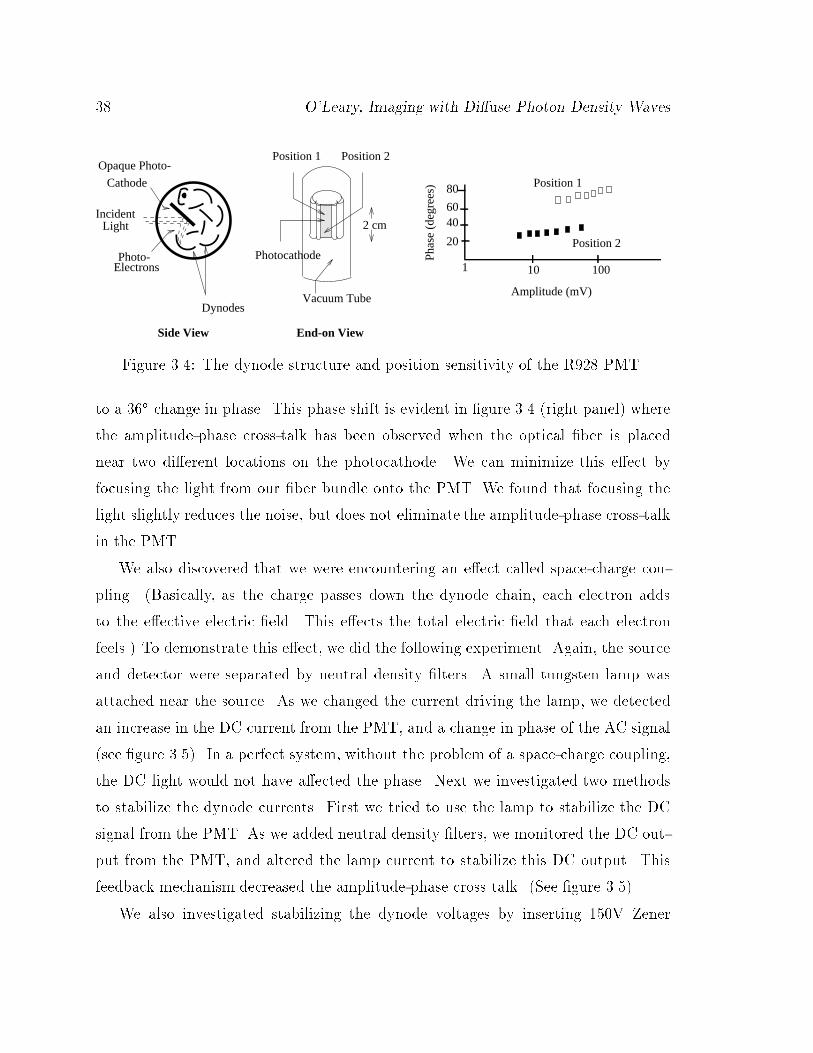
38 O'Leary, Imaging with Di�use Photon Density Waves
End-on ViewSide View
Vacuum Tube
Position 2Position 1
Photocathode
2 cm
Cathode
IncidentLight
Photo-Electrons
Opaque Photo-
Phas
e (d
egre
es)
10 100
Amplitude (mV)
80
6040
20
1
Position 2
Position 1
Dynodes
Figure 3.4: The dynode structure and position sensitivity of the R928 PMT.
to a 36� change in phase. This phase shift is evident in �gure 3.4 (right panel) where
the amplitude-phase cross-talk has been observed when the optical �ber is placed
near two di�erent locations on the photocathode. We can minimize this e�ect by
focusing the light from our �ber bundle onto the PMT. We found that focusing the
light slightly reduces the noise, but does not eliminate the amplitude-phase cross-talk
in the PMT.
We also discovered that we were encountering an e�ect called space-charge cou-
pling. (Basically, as the charge passes down the dynode chain, each electron adds
to the e�ective electric �eld. This e�ects the total electric �eld that each electron
feels.) To demonstrate this e�ect, we did the following experiment. Again, the source
and detector were separated by neutral density �lters. A small tungsten lamp was
attached near the source. As we changed the current driving the lamp, we detected
an increase in the DC current from the PMT, and a change in phase of the AC signal
(see �gure 3.5). In a perfect system, without the problem of a space-charge coupling,
the DC light would not have a�ected the phase. Next we investigated two methods
to stabilize the dynode currents. First we tried to use the lamp to stabilize the DC
signal from the PMT. As we added neutral density �lters, we monitored the DC out-
put from the PMT, and altered the lamp current to stabilize this DC output. This
feedback mechanism decreased the amplitude-phase cross talk. (See �gure 3.5).
We also investigated stabilizing the dynode voltages by inserting 150V Zener
Hardware Speci�cations 39
SupplyCurrentVariable
Photon ModulationDevice
FiltersNeutral Density
ammeterDC
Detector Fiber
Feedback Loop
Tungston Lamp
Source Fiber
PMT 128
132
136
140
144
0 1 2 3 4 5 6
With FeedbackNo feedback
number of ND filters
Pha
se (
degr
ees)
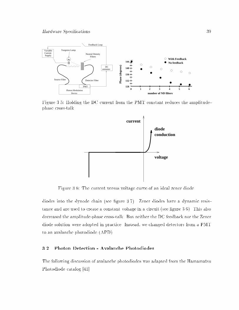
Figure 3.5: Holding the DC current from the PMT constant reduces the amplitude-phase cross-talk.
diodeconduction
current
voltage
Figure 3.6: The current versus voltage curve of an ideal zener diode.
diodes into the dynode chain (see �gure 3.7). Zener diodes have a dynamic resis-
tance and are used to create a constant voltage in a circuit (see �gure 3.6). This also
decreased the amplitude-phase cross-talk. But neither the DC feedback nor the Zener
diode solution were adopted in practice. Instead, we changed detectors from a PMT
to an avalanche photodiode (APD).
3.2 Photon Detection - Avalanche Photodiodes
The following discussion of avalanche photodiodes was adapted from the Hamamatsu
Photodiode catalog [41].
40 O'Leary, Imaging with Di�use Photon Density Waves
GNDGND
-HV
AnodeCathode
0
16
12
8
4
0.4 0.6 0.8 1.0 1.2 1.4 1.6 1.8
With diodeNo diode
Optical Density
Phas
e (d
egre
es)
GNDGND
-HV
AnodeCathode
No Diode
With Diode
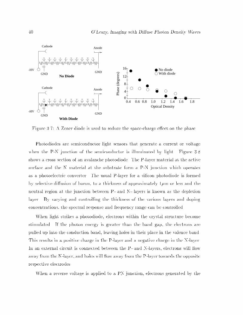
Figure 3.7: A Zener diode is used to reduce the space-charge e�ect on the phase.
Photodiodes are semiconductor light sensors that generate a current or voltage
when the P-N junction of the semiconductor is illuminated by light. Figure 3.8
shows a cross section of an avalanche photodiode. The P-layer material at the active
surface and the N material at the substrate form a P-N junction which operates
as a photoelectric converter. The usual P-layer for a silicon photodiode is formed
by selective di�usion of boron, to a thickness of approximately 1�m or less and the
neutral region at the junction between P- and N- layers is known as the depletion
layer. By varying and controlling the thickness of the various layers and doping
concentrations, the spectral response and frequency range can be controlled.
When light strikes a photodiode, electrons within the crystal structure become
stimulated. If the photon energy is greater than the band gap, the electrons are
pulled up into the conduction band, leaving holes in their place in the valence band.
This results in a positive charge in the P-layer and a negative charge in the N-layer.
In an external circuit is connected between the P- and N-layers, electrons will ow
away from the N-layer, and holes will ow away from the P-layer towards the opposite
respective electrodes.
When a reverse voltage is applied to a PN junction, electrons generated by the

Hardware Speci�cations 41
Active area 0.19 mm2
Window material borosilicate glass
Peak Wavelength 800nm
Anode to Cathode Voltage (max) 200 V
Current ampli�cation (without external
ampli�er)
1� 102
Dark current 0.1 nA
Frequency range (equivalent to rise time) 1MHz - 1GHz
Table 3.2: Speci�cations of the Hamamatsu C5658 Avalanche photodiode.
incident light collide with atoms in the �eld and produce secondary electrons. This
process occurs repeatedly. This is known as the avalanche e�ect, and since it results
in the signal being ampli�ed, this type of device is ideally suited for detection of low
light levels.
The APD we used was a Hamamatsu C5658, and the speci�cations are given in
table 3.2. This particular APD has a built-in bias supply, current to voltage converter
and a low noise, broad band ampli�er.
Because the APD is compact, there are virtually no path length variations as in
the photomultiplier tube. We were not able to detect any amplitude-phase cross-talk
using the APD, although Yokoyama et al. [42] have detected a small amplitude-phase
cross-talk in the APD at 1 GHz. In addition, the sensitivity range of the APD extends
much further into the infra-red (400 nm - 1000 nm for the APD, (�gure 3.9,) 400 nm
- 800 nm for the PMT). The disadvantages of the APD are its small active area (0.5
mm) and low gain (with a built in low noise ampli�er the ADP module gain is 105
compared to the PMT gain of 106). Finally, the response of the APD is fast enough
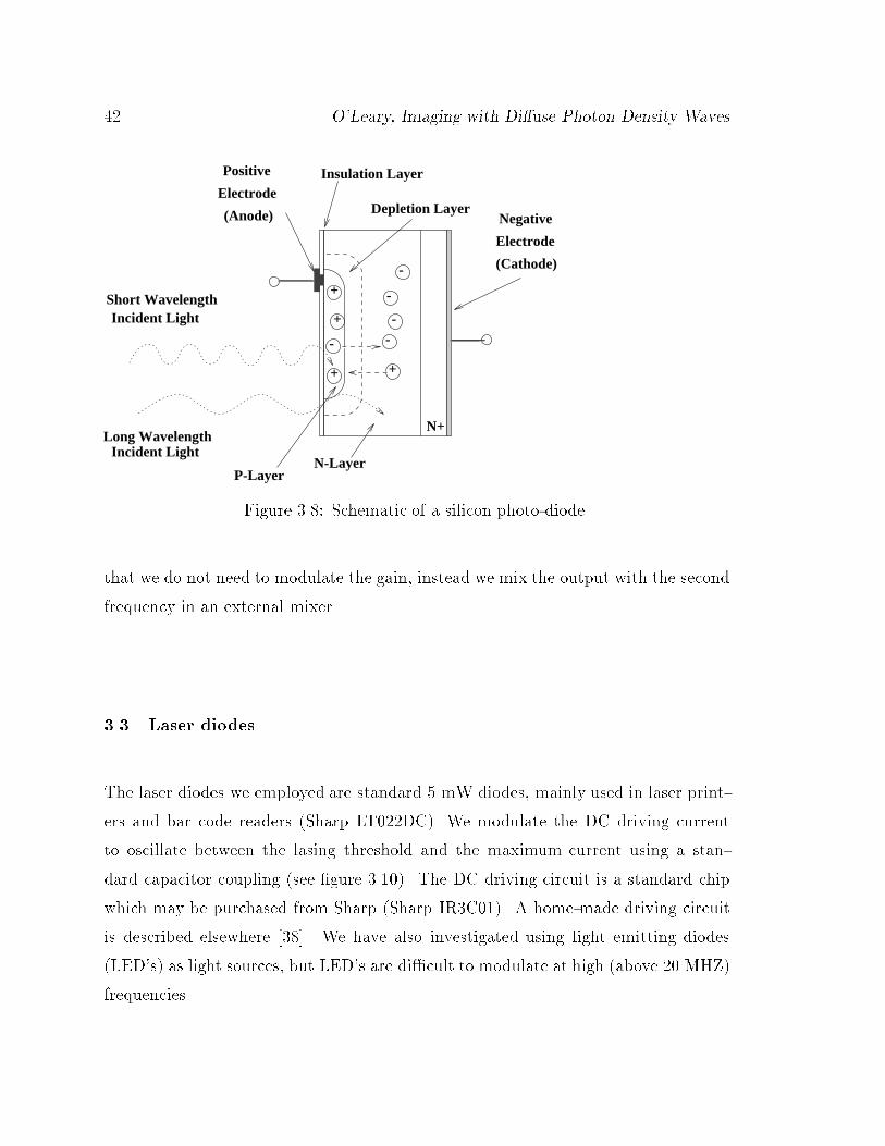
42 O'Leary, Imaging with Di�use Photon Density Waves
-
-
(Anode)
-
-
Electrode
-
+
+
+
Negative
Electrode
+
(Cathode)
Positive
N-Layer
Insulation Layer
Depletion Layer
N+Long Wavelength
Short WavelengthIncident Light
Incident Light
P-Layer
Figure 3.8: Schematic of a silicon photo-diode.
that we do not need to modulate the gain, instead we mix the output with the second
frequency in an external mixer.
3.3 Laser diodes
The laser diodes we employed are standard 5 mW diodes, mainly used in laser print-
ers and bar code readers (Sharp LT022DC). We modulate the DC driving current
to oscillate between the lasing threshold and the maximum current using a stan-
dard capacitor coupling (see �gure 3.10). The DC driving circuit is a standard chip
which may be purchased from Sharp (Sharp IR3C01). A home-made driving circuit
is described elsewhere [38]. We have also investigated using light emitting diodes
(LED's) as light sources, but LED's are di�cult to modulate at high (above 20 MHZ)
frequencies.
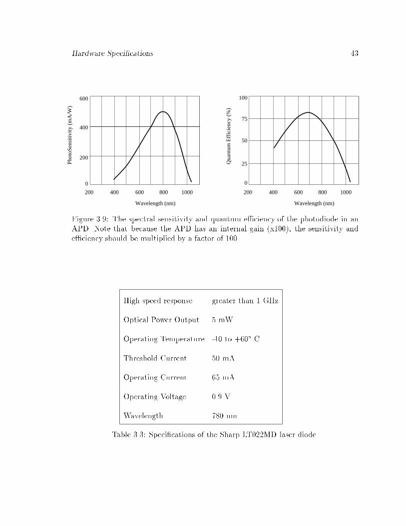
Hardware Speci�cations 43
200 400 600 800 1000
0
100
75
25
50
200 400 600 800 1000
0
600
400
200
Wavelength (nm)
Qua
ntum
Eff
icie
ncy
(%)
Wavelength (nm)
Phot
oSen
sitiv
ity (
mA
/W)
Figure 3.9: The spectral sensitivity and quantum e�ciency of the photodiode in anAPD. Note that because the APD has an internal gain (x100), the sensitivity ande�ciency should be multiplied by a factor of 100.
High speed response greater than 1 GHz
Optical Power Output 5 mW
Operating Temperature -10 to +60� C
Threshold Current 50 mA
Operating Current 65 mA
Operating Voltage 0.9 V
Wavelength 780 nm
Table 3.3: Speci�cations of the Sharp LT022MD laser diode.
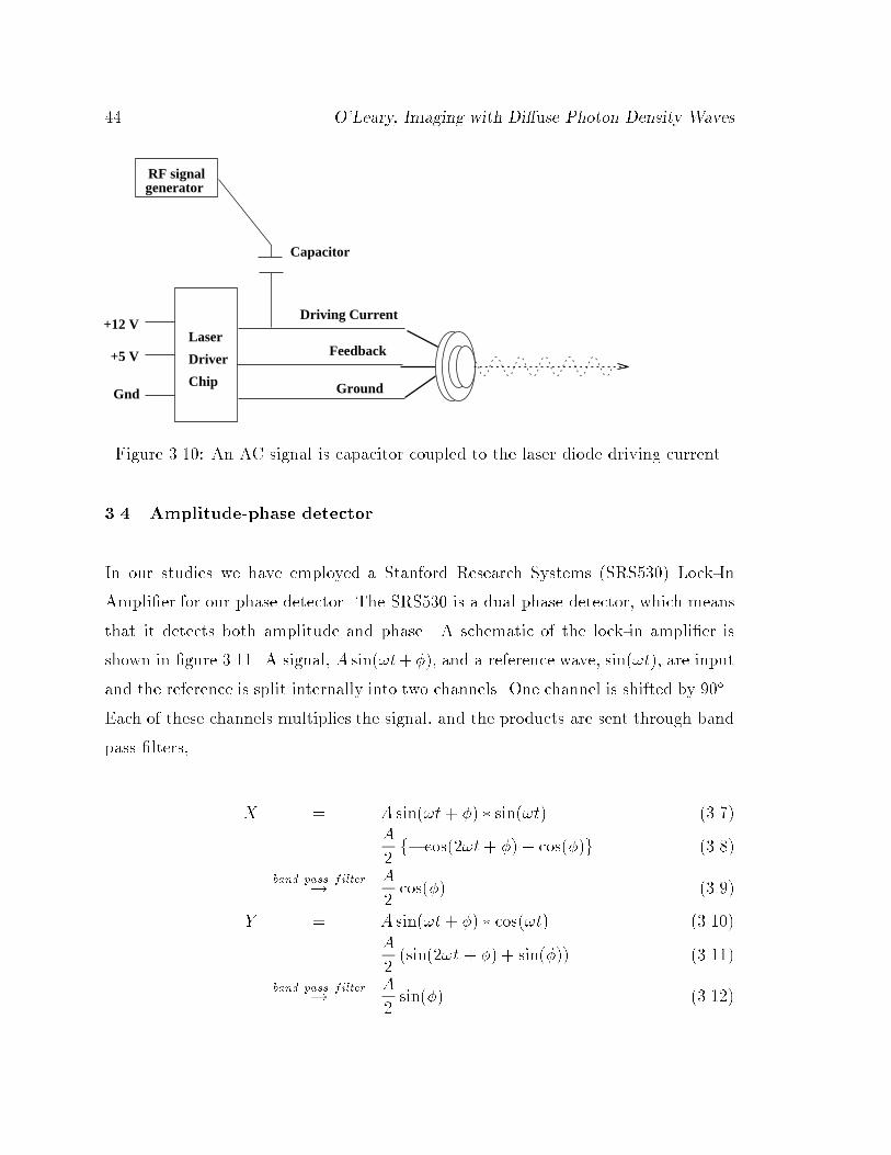
44 O'Leary, Imaging with Di�use Photon Density Waves
+12 V
+5 V
Gnd Ground
FeedbackLaser
Driver
Chip
Driving Current
Capacitor
generatorRF signal
Figure 3.10: An AC signal is capacitor coupled to the laser diode driving current.
3.4 Amplitude-phase detector
In our studies we have employed a Stanford Research Systems (SRS530) Lock-In
Ampli�er for our phase detector. The SRS530 is a dual phase detector, which means
that it detects both amplitude and phase. A schematic of the lock-in ampli�er is
shown in �gure 3.11. A signal, A sin(!t+�), and a reference wave, sin(!t), are input
and the reference is split internally into two channels. One channel is shifted by 90� .
Each of these channels multiplies the signal, and the products are sent through band
pass �lters,
X = A sin(!t+ �) � sin(!t) (3.7)
=A
2f� cos(2!t+ �) + cos(�)g (3.8)
band pass filter!
A
2cos(�) (3.9)
Y = A sin(!t+ �) � cos(!t) (3.10)
=A
2(sin(2!t + �) + sin(�)) (3.11)
band pass filter!
A
2sin(�) (3.12)
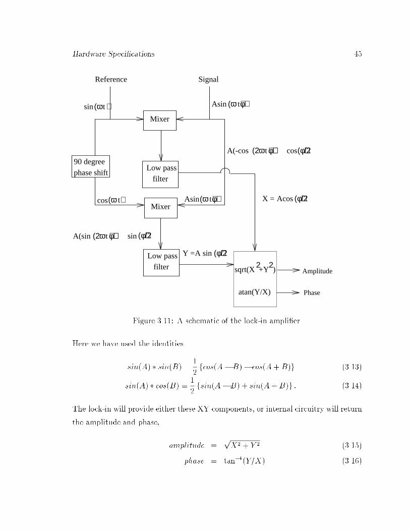
Hardware Speci�cations 45
(2ω +φ)+
(φ))/2
Low passfilter
Mixer
Mixert(ω ) (ω +φ)tAsin
sin (ω )t (ω +φ)tAsin
2 2sqrt(X +Y )
(2ω +φ)+t
X = Acos (φ))/2
A sinY = (φ))/2
A(sin
tA(-cos cos(φ))/2
Reference
Low passfilter
cos
atan(Y/X)
Amplitude
Phase
Signal
phase shift
sin
90 degree
Figure 3.11: A schematic of the lock-in ampli�er.
Here we have used the identities
sin(A) � sin(B) =1
2fcos(A�B)� cos(A+B)g (3.13)
sin(A) � cos(B) =1
2fsin(A�B) + sin(A+B)g : (3.14)
The lock-in will provide either these XY components, or internal circuitry will return
the amplitude and phase,
amplitude =pX2 + Y 2 (3.15)
phase = tan�1(Y=X) (3.16)
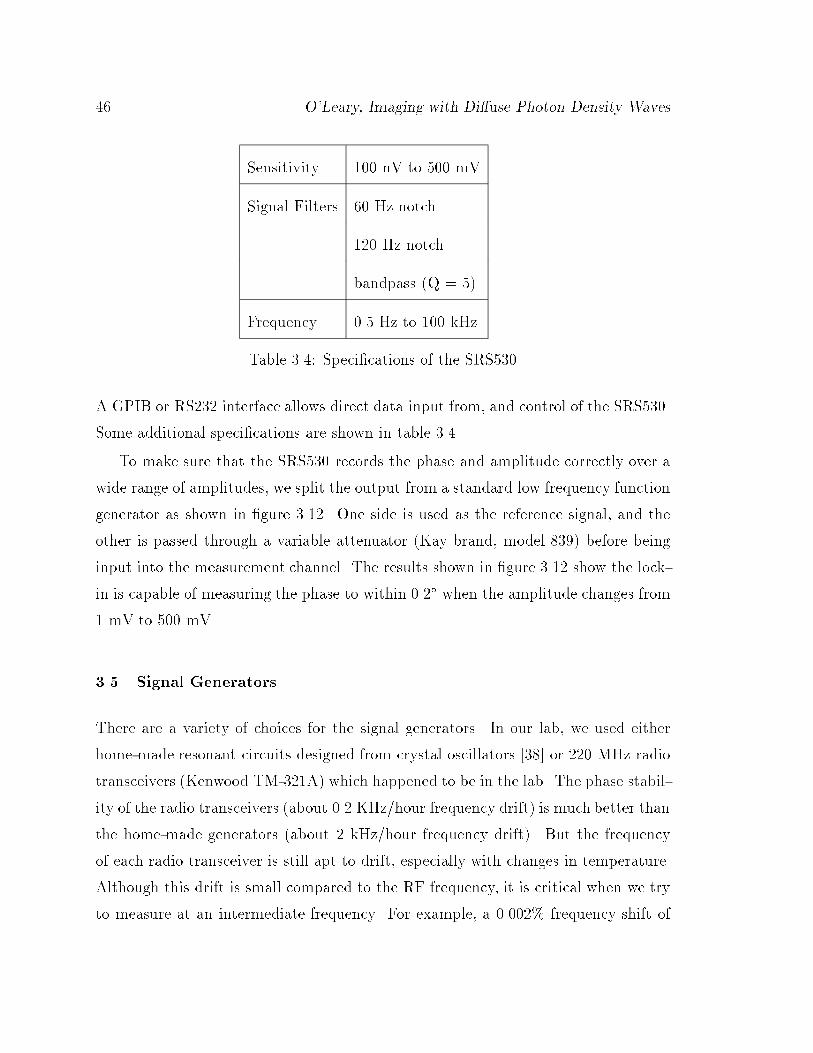
46 O'Leary, Imaging with Di�use Photon Density Waves
Sensitivity 100 nV to 500 mV
Signal Filters 60 Hz notch
120 Hz notch
bandpass (Q = 5)
Frequency 0.5 Hz to 100 kHz
Table 3.4: Speci�cations of the SRS530
A GPIB or RS232 interface allows direct data input from, and control of the SRS530.
Some additional speci�cations are shown in table 3.4.
To make sure that the SRS530 records the phase and amplitude correctly over a
wide range of amplitudes, we split the output from a standard low frequency function
generator as shown in �gure 3.12. One side is used as the reference signal, and the
other is passed through a variable attenuator (Kay brand, model 839) before being
input into the measurement channel. The results shown in �gure 3.12 show the lock-
in is capable of measuring the phase to within 0.2� when the amplitude changes from
1 mV to 500 mV.
3.5 Signal Generators
There are a variety of choices for the signal generators. In our lab, we used either
home-made resonant circuits designed from crystal oscillators [38] or 220 MHz radio
transceivers (Kenwood TM-321A) which happened to be in the lab. The phase stabil-
ity of the radio transceivers (about 0.2 KHz/hour frequency drift) is much better than
the home-made generators (about 2 kHz/hour frequency drift). But the frequency
of each radio transceiver is still apt to drift, especially with changes in temperature.
Although this drift is small compared to the RF frequency, it is critical when we try
to measure at an intermediate frequency. For example, a 0.002% frequency shift of
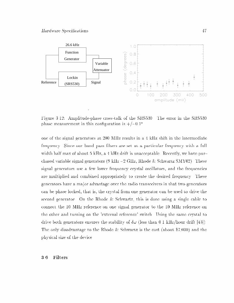
Hardware Speci�cations 47
(SRS530)
Attenuator
Lockin
Variable
Function
Generator
Reference Signal
26.6 kHz
.
Figure 3.12: Amplitude-phase cross-talk of the SRS530. The error in the SRS530phase measurement in this con�guration is +/- 0.1� .
one of the signal generators at 200 MHz results in a 4 kHz shift in the intermediate
frequency. Since our band pass �lters are set at a particular frequency with a full
width half max of about 5 kHz, a 4 kHz drift is unacceptable. Recently, we have pur-
chased variable signal generators (9 kHz - 2 GHz, Rhode & Schwartz SMY02). These
signal generators use a few lower frequency crystal oscillators, and the frequencies
are multiplied and combined appropriately to create the desired frequency. These
generators have a major advantage over the radio transceivers in that two generators
can be phase locked, that is, the crystal from one generator can be used to drive the
second generator. On the Rhode & Schwartz, this is done using a single cable to
connect the 10 MHz reference on one signal generator to the 10 MHz reference on
the other and turning on the 'external reference' switch. Using the same crystal to
drive both generators ensures the stability of �! (less than 0.1 kHz/hour drift [43]).
The only disadvantage to the Rhode & Schwartz is the cost (about $7,000) and the
physical size of the device.
3.6 Filters
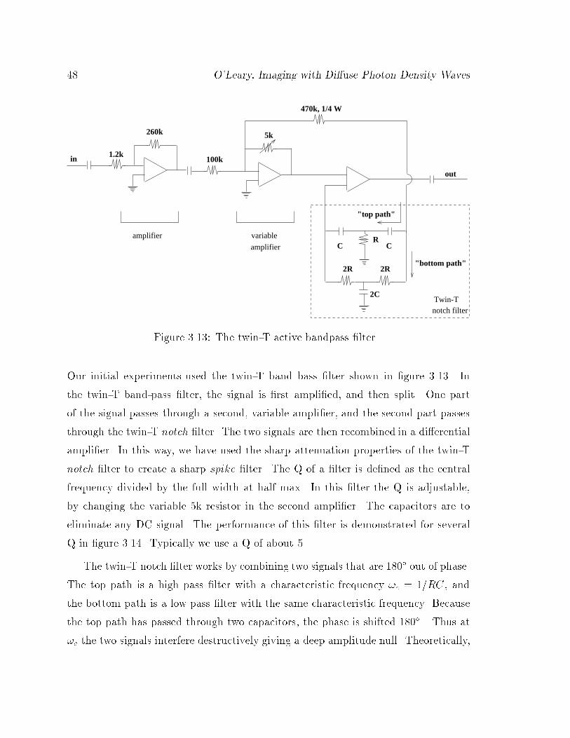
48 O'Leary, Imaging with Di�use Photon Density Waves
amplifier
variable
Twin-T notch filter
R
2C
5k
in
out
1.2k
470k, 1/4 W
amplifier
100k
260k
C C
2R 2R
"top path"
"bottom path"
Figure 3.13: The twin-T active bandpass �lter.
Our initial experiments used the twin-T band bass �lter shown in �gure 3.13. In
the twin-T band-pass �lter, the signal is �rst ampli�ed, and then split. One part
of the signal passes through a second, variable ampli�er, and the second part passes
through the twin-T notch �lter. The two signals are then recombined in a di�erential
ampli�er. In this way, we have used the sharp attenuation properties of the twin-T
notch �lter to create a sharp spike �lter. The Q of a �lter is de�ned as the central
frequency divided by the full width at half max. In this �lter the Q is adjustable,
by changing the variable 5k resistor in the second ampli�er. The capacitors are to
eliminate any DC signal. The performance of this �lter is demonstrated for several
Q in �gure 3.14. Typically we use a Q of about 5.
The twin-T notch �lter works by combining two signals that are 180� out of phase.
The top path is a high pass �lter with a characteristic frequency !c = 1=RC, and
the bottom path is a low pass �lter with the same characteristic frequency. Because
the top path has passed through two capacitors, the phase is shifted 180� . Thus at
!c the two signals interfere destructively giving a deep amplitude null. Theoretically,
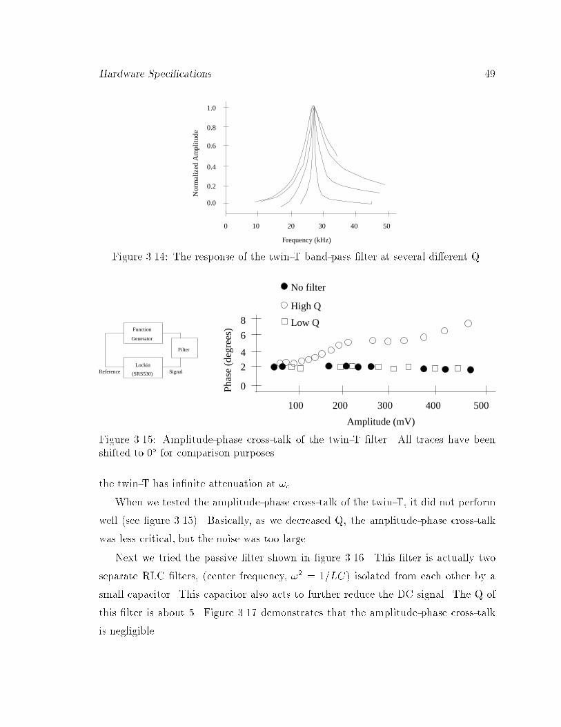
Hardware Speci�cations 49
0 10 20 30 40 50
1.0
0.8
0.6
0.4
0.2
0.0N
orm
aliz
ed A
mpl
itude
Frequency (kHz)
Figure 3.14: The response of the twin-T band-pass �lter at several di�erent Q.
(SRS530)
Generator
Function
LockinReference Signal
Filter
0
2
4
6
8
100 200 300 400 500
High Q
No filter
Low Q
Phas
e (d
egre
es)
Amplitude (mV)
Figure 3.15: Amplitude-phase cross-talk of the twin-T �lter. All traces have beenshifted to 0� for comparison purposes.
the twin-T has in�nite attenuation at !c.
When we tested the amplitude-phase cross-talk of the twin-T, it did not perform
well (see �gure 3.15). Basically, as we decreased Q, the amplitude-phase cross-talk
was less critical, but the noise was too large.
Next we tried the passive �lter shown in �gure 3.16. This �lter is actually two
separate RLC �lters, (center frequency, !2 = 1=LC) isolated from each other by a
small capacitor. This capacitor also acts to further reduce the DC signal. The Q of
this �lter is about 5. Figure 3.17 demonstrates that the amplitude-phase cross-talk
is negligible.
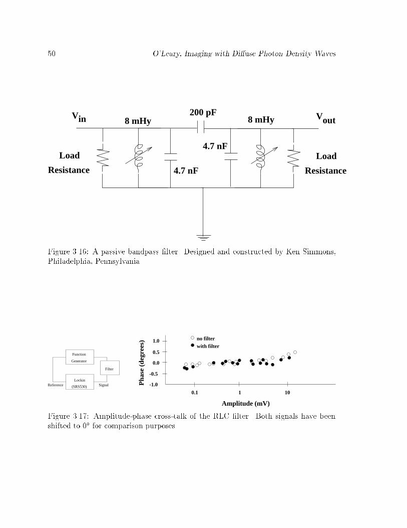
50 O'Leary, Imaging with Di�use Photon Density Waves
Load
Resistance
Load
Resistance
200 pFVin Vout8 mHy 8 mHy
4.7 nF
4.7 nF
Figure 3.16: A passive bandpass �lter. Designed and constructed by Ken Simmons,Philadelphia, Pennsylvania.
(SRS530)
Generator
Function
LockinReference Signal
Filter
-1.0
-0.5
0.5
1.0
0.0
10.1 10
no filterwith filter
Amplitude (mV)
Pha
se (
degr
ees)
Figure 3.17: Amplitude-phase cross-talk of the RLC �lter. Both signals have beenshifted to 0� for comparison purposes.
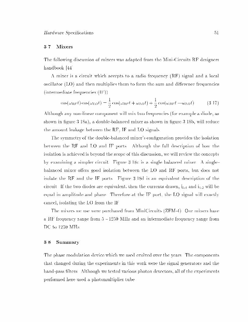
Hardware Speci�cations 51
3.7 Mixers
The following discussion of mixers was adapted from the Mini-Circuits RF designers
handbook [44].
A mixer is a circuit which accepts to a radio frequency (RF) signal and a local
oscillator (LO) and then multiplies them to form the sum and di�erence frequencies
(intermediate frequencies (IF)).
cos(!RF t) cos(!LOt) =1
2cos(!RF t+ !LOt) +
1
2cos(!RF t� !LOt) (3.17)
Although any non-linear component will mix two frequencies (for example a diode, as
shown in �gure 3.18a), a double-balanced mixer as shown in �gure 3.18b, will reduce
the amount leakage between the RF, IF and LO signals.
The symmetry of the double-balanced mixer's con�guration provides the isolation
between the RF and LO and IF ports. Although the full description of how the
isolation is achieved is beyond the scope of this discussion, we will review the concepts
by examining a simpler circuit. Figure 3.18c is a single balanced mixer. A single-
balanced mixer o�ers good isolation between the LO and RF ports, but does not
isolate the RF and the IF ports. Figure 3.18d is an equivalent description of the
circuit. If the two diodes are equivalent, then the currents drawn, ilo1 and ilo2 will be
equal in amplitude and phase. Therefore at the IF port, the LO signal will exactly
cancel, isolating the LO from the IF.
The mixers we use were purchased from MiniCircuits (ZFM-4). Our mixers have
a RF frequency range from 5 - 1250 MHz and an intermediate frequency range from
DC to 1250 MHz.
3.8 Summary
The phase modulation device which we used evolved over the years. The components
that changed during the experiments in this work were the signal generators and the
band-pass �lters. Although we tested various photon detectors, all of the experiments
performed here used a photomultiplier tube.
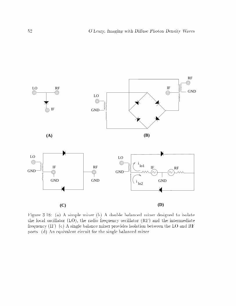
52 O'Leary, Imaging with Di�use Photon Density Waves
IF
GND
LO
GND
GND
RF
GNDIF
LO
GND
RF
LO RF
IF
(A) (B)
(C) (D)
LO
GNDRFIF
GND
i
i
lo1
lo2
Figure 3.18: (a) A simple mixer (b) A double balanced mixer designed to isolatethe local oscillator (LO), the radio frequency oscillator (RF) and the intermediatefrequency (IF). (c) A single balance mixer provides isolation between the LO and RFports. (d) An equivalent circuit for the single balanced mixer.
Hardware Speci�cations 53
The initial experiments demonstrating the existence and properties of DPDW
(presented in chapter 2) used a system composed of the twin-T band-pass �lter and
the home-made radio oscillators. Most of the absorption and scattering images were
created using the radio transceivers and the twin-T band-pass �lters. The absorption
calibration curve was created using the radio transceivers and the LC band-pass �lters.

54 O'Leary, Imaging with Di�use Photon Density Waves
Chapter 4
Imaging the Absorption Coe�cient
Near infrared di�using light probes o�er new possibilities for medical imaging. Appli-
cations include non-invasive measurement of tissue oxygenation, and tumor detection
and characterization [45]. Although investigators have determined the bulk optical
properties based on a homogeneous model, direct imaging of the optical properties
of heterogeneous tissue is an important potential improvement that has only recently
been considered [46, 47]. It is expected that these images will lead to a more accu-
rate representation of the optical properties for tissue characterization and functional
imaging.
In this chapter we will assume that only the absorption coe�cient varies with
position. The other optical properties, such as the scattering coe�cient, are assumed
to be constant. To investigate the passage of photons through heterogeneous media
we �rst write down the heterogeneous di�usion equation, and then generate solutions
to this equation using two methods. The �rst involves a linear or Born expansion of
the light energy density changes, and the second is an exponential or Rytov expansion
of the light energy density changes.
We next discuss methods for inverting these solutions to obtain images of the
medium. Again, we have investigated two di�erent methods: the �rst is a matrix
inversion, singular value decomposition (SVD), and the second is an algebraic re-
construction technique (SIRT). We present experimental results which demonstrate
the feasibility of image reconstruction and characterization of the optical properties.
Finally, we suggest an algorithm which exploits a high resolution imaging modality
55
56 O'Leary, Imaging with Di�use Photon Density Waves
such as MRI, x-ray tomography or ultra-sound to improve tissue characterization.
4.1 The Heterogeneous Di�usion Equation
The systems we are concerned with in this chapter have an absorption coe�cient,
�a(r) which may be divided into two components, the background, or homogeneous
component, �oa, and the spatially varying part ��a(r);
�a(r) = �oa + ��a(r): (4.1)
When we substitute equation 4.1 into the di�usion equation or its related Helmholtz
equation:
�Dr2Uac(r) + (�i! + v�a)U(r) = �A�(rs); (4.2)
(r2 + k2)U(r) = A�(rs)=D: (4.3)
we arrive at the heterogeneous equation for the light energy density at r from a source
at rs, A�(rs);
hr
2 + k2 +O(r)iU(r; rs) = A�(rs)=D; (4.4)
O(r) = v��a(r)=D: (4.5)
To solve this heterogeneous di�usion equation, we will explore both the Born and the
Rytov formulations. The following discussion is an adaptation of the discussion by
Kak et al. [48].
4.2 Born Approximation
In the Born expansion we divide the photon density from a source at rs measured at
a position r, into a linear superposition of its incident (homogeneous) and scattered
(heterogeneous) parts;
U(r; rs) = Uo(r; rs) + Usc(r; rs): (4.6)
Imaging Absorption 57
The heterogeneous di�usion equation (equation 4.4) becomes
hr
2 + k2 +O(r)i[Uo(r; rs) + Usc(r; rs)] = �A�(rs)=D; (4.7)
If we subtract o� the homogeneous Helmholtz equation,
(r2 + k2)Uo(r; rs) = �A�(rs)=D (4.8)
then we are left with the following heterogeneous Helmholtz equation for Usc.
(r2 + k20)Usc(r; rs) = �O(r) [Uo(r; rs) + Usc(r; rs)] (4.9)
We next convolve this di�erential equation with the appropriate Green function so-
lution to the Helmholtz equation, to arrive at the following integral solution for Usc;
Usc(rd; rs) = �
ZG(r� rd)O(r) [Uo(r; rs) + Usc(r; rs)]d
3r; (4.10)
G(r� rd) = exp(ikjr� rdj)=4�jr� rdj: (4.11)
The integral is over the entire sample volume. We now make the Born approximation,
i.e. we assume that
Usc(r)� Uo(r); (4.12)
and we can write down an explicit solution for the scattered DPDW in a heterogeneous
medium,
Usc(rd; rs) = �
ZG(r� rd)O(r)Uo(r; rs) d
3r (4.13)
with
U(rd; rs) = Uo(rd; rs) + Usc(rd; rs) (4.14)
We will refer to this solution (equation 4.13) as the Born solution. Figure 4.1 demon-
strates the components of the Born solution. One can think of this solution for Usc
as the number of photons which pass from the source (rs) to some position r, scat-
ter with an amplitude proportional to ��a, and then travel from the position r to a
detector at rd.
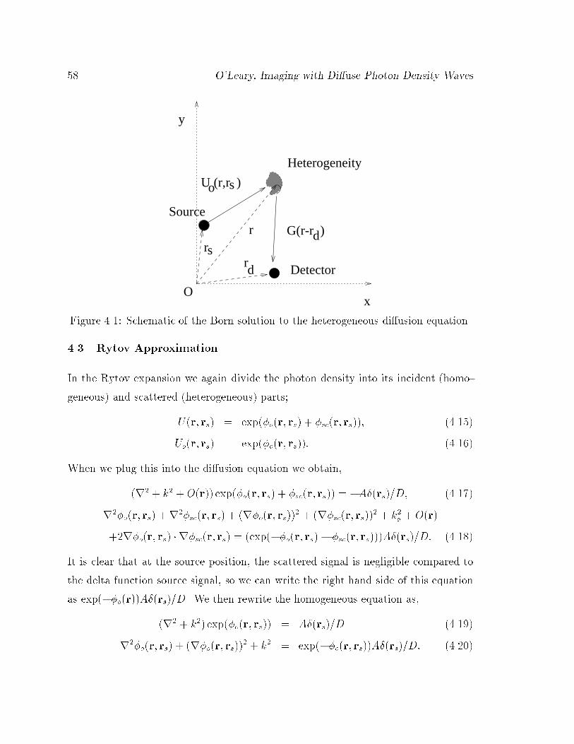
58 O'Leary, Imaging with Di�use Photon Density Waves
dr
r
O
Detector
Source
G(r-r )
U (r,r )o
d
x
y
s
rs
Heterogeneity
Figure 4.1: Schematic of the Born solution to the heterogeneous di�usion equation.
4.3 Rytov Approximation
In the Rytov expansion we again divide the photon density into its incident (homo-
geneous) and scattered (heterogeneous) parts;
U(r; rs) = exp(�o(r; rs) + �sc(r; rs)); (4.15)
Uo(r; rs) = exp(�o(r; rs)): (4.16)
When we plug this into the di�usion equation we obtain,
(r2 + k2 +O(r)) exp(�o(r; rs) + �sc(r; rs)) = �A�(rs)=D; (4.17)
r2�o(r; rs) +r
2�sc(r; rs) + (r�o(r; rs))2 + (r�sc(r; rs))
2 + k2o +O(r)
+2r�o(r; rs) � r�sc(r; rs) = (exp(��o(r; rs)� �sc(r; rs)))A�(rs)=D: (4.18)
It is clear that at the source position, the scattered signal is negligible compared to
the delta function source signal, so we can write the right hand side of this equation
as exp(��o(r))A�(rs)=D. We then rewrite the homogeneous equation as,
(r2 + k2) exp(�o(r; rs)) = A�(rs)=D (4.19)
r2�o(r; rs) + (r�o(r; rs))
2 + k2 = exp(��o(r; rs))A�(rs)=D: (4.20)
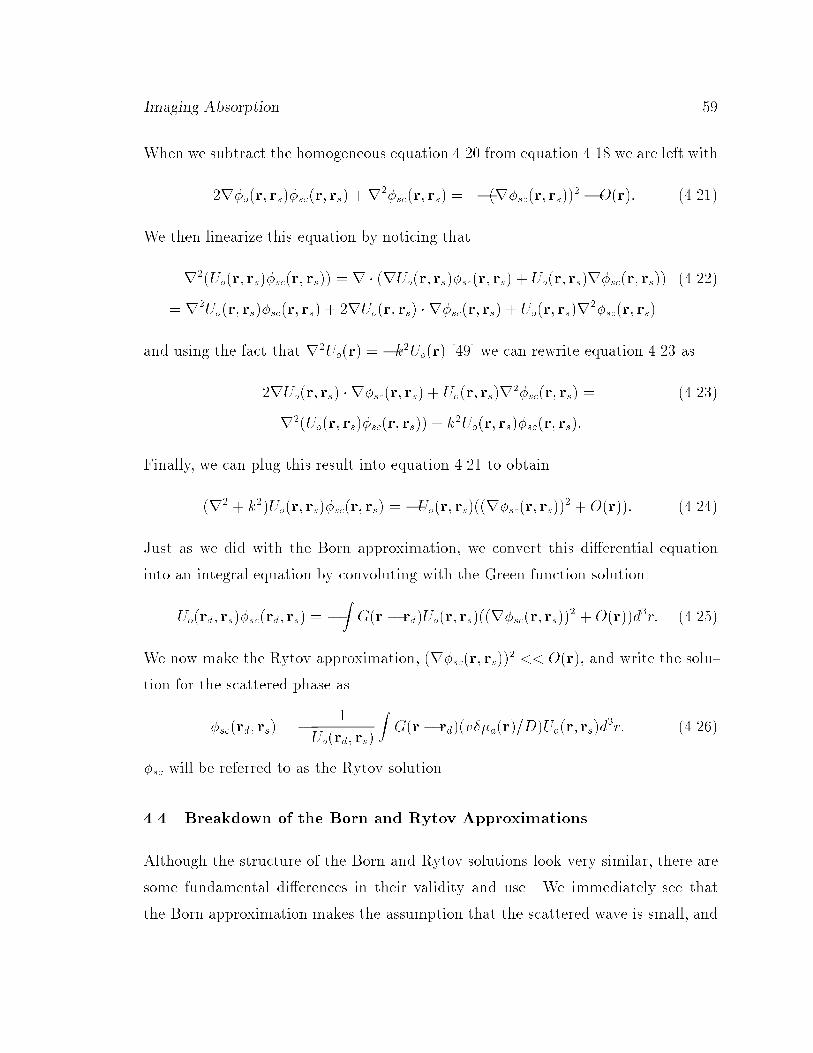
Imaging Absorption 59
When we subtract the homogeneous equation 4.20 from equation 4.18 we are left with
2r�o(r; rs)�sc(r; rs) +r2�sc(r; rs) = �(r�sc(r; rs))2 �O(r): (4.21)
We then linearize this equation by noticing that
r2(Uo(r; rs)�sc(r; rs)) = r � (rUo(r; rs)�sc(r; rs) + Uo(r; rs)r�sc(r; rs)) (4.22)
= r2Uo(r; rs)�sc(r; rs) + 2rUo(r; rs) � r�sc(r; rs) + Uo(r; rs)r
2�sc(r; rs)
and using the fact that r2Uo(r) = �k2Uo(r) [49] we can rewrite equation 4.23 as
2rUo(r; rs) � r�sc(r; rs) + Uo(r; rs)r2�sc(r; rs) = (4.23)
r2(Uo(r; rs)�sc(r; rs)) + k2Uo(r; rs)�sc(r; rs):
Finally, we can plug this result into equation 4.21 to obtain
(r2 + k2)Uo(r; rs)�sc(r; rs) = �Uo(r; rs)((r�sc(r; rs))2 +O(r)): (4.24)
Just as we did with the Born approximation, we convert this di�erential equation
into an integral equation by convoluting with the Green function solution.
Uo(rd; rs)�sc(rd; rs) = �
ZG(r � rd)Uo(r; rs)((r�sc(r; rs))
2 +O(r))d3r: (4.25)
We now make the Rytov approximation, (r�sc(r; rs))2 << O(r), and write the solu-
tion for the scattered phase as
�sc(rd; rs) = �1
Uo(rd; rs)
ZG(r� rd)(v��a(r)=D)Uo(r; rs)d
3r: (4.26)
�sc will be referred to as the Rytov solution.
4.4 Breakdown of the Born and Rytov Approximations
Although the structure of the Born and Rytov solutions look very similar, there are
some fundamental di�erences in their validity and use. We immediately see that
the Born approximation makes the assumption that the scattered wave is small, and
60 O'Leary, Imaging with Di�use Photon Density Waves
5.04.03.02.01.00.00.0
0.2
0.4
0.6
0.8
1.0
Rytov
Born
reco
nstr
ucte
d ab
sorp
tion
(1/c
m)
true absorption (1/cm)
1/l* = 10.0 1/cmabsorption varies
absorption = 0.05 1/cm
1/l* = 10.0 1/cm
Detector
Source
Figure 4.2: A comparison of the Born and Rytov approximations. A 1.0 cm diametersphere is embedded in a medium with an absorption of 0.03 cm�1 and a reducedscattering coe�cient of 10.0 cm�1. Although a cylindrical region was reconstructed,an in�nite model was used for both the forward and inverse problems.
the scattered wave scales approximately linearly with the absorption. In biological
tissue we are interested in imaging absorption values which vary from about 0.02
cm�1 to 0.30 cm�1. In fact, this linear assumption will break down for absorption
di�erences greater than about 0.10 cm�1, well within our region of interest. The
Rytov approximation does not place a restriction on the magnitude of the scattered
wave change, but rather assumes that the scattered �eld is slowly varying. Figure
4.2 demonstrates the breakdown of each approximation in the context of an isolated
spherical heterogeneity. We see that the Rytov approximation is much more suitable
for most biological situations. These and other di�erences will be discussed in section
4.8 and chapter 6.
4.5 Inverting the Solutions to the Heterogeneous Di�usion Equation
Our goal is to use either the Born or Rytov equations to solve for the absorption as a
function of position within the medium. Thus we must invert the integral equations
Imaging Absorption 61
(4.13, 4.26). There are many methods available to �nd the best solution to the inverse
problem. But care must be taken since the integral equation is a Fredholm integral
of the �rst kind (FI) and is highly susceptible to high frequency noise. A FI is an
equation of the form
u(x) =Z b
ak(x; s)�(s)ds: (4.27)
The di�culty in solving a FI for � arises from the instability of the inverse operator.
Certain high frequency oscillatory noise in a solution may be screened out by the
integral operator, giving a result which is very close to the left hand side. For example,
if th correct solution to our problem is �(s), consider the residual of another solution
�(s) + ��(s) where
��(s) = exp(i!s) (4.28)
The residual, �u(x) that this alternate solution adds to the measurements is
�u(x) =Z b
ak(x; s)��(s)ds (4.29)
=Z b
ak(x; s) exp(iws)ds: (4.30)
If we integrate by parts,
�u(x) =1
i!k(x; s)��(s)
����a
b
�1
i!
Z b
a
@k(x; s)
@sexp(iws)ds (4.31)
we see that the residual is of order 1=!. Thus high frequency solutions for � will
contribute little to the measurement, but can contribute signi�cantly to the the image.
There are regularization schemes, such as Tikhonov regularization, which reduce
the e�ect of high frequency noise on the reconstructed image. To invert the following
equation;
~u = ~A~x (4.32)
we would minimize the norm
jj~u� ~A~xjj: (4.33)
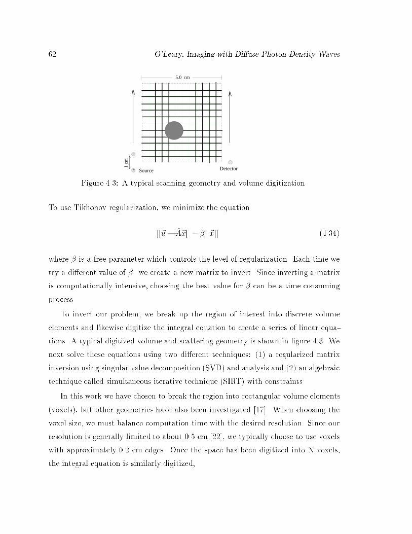
62 O'Leary, Imaging with Di�use Photon Density Waves
5.0 cm
1 cm
-
+ DetectorSource
Figure 4.3: A typical scanning geometry and volume digitization.
To use Tikhonov regularization, we minimize the equation
jj~u� ~A~xjj+ �jj~xjj (4.34)
where � is a free parameter which controls the level of regularization. Each time we
try a di�erent value of �. we create a new matrix to invert. Since inverting a matrix
is computationally intensive, choosing the best value for � can be a time consuming
process.
To invert our problem, we break up the region of interest into discrete volume
elements and likewise digitize the integral equation to create a series of linear equa-
tions. A typical digitized volume and scattering geometry is shown in �gure 4.3. We
next solve these equations using two di�erent techniques: (1) a regularized matrix
inversion using singular value decomposition (SVD) and analysis and (2) an algebraic
technique called simultaneous iterative technique (SIRT) with constraints.
In this work we have chosen to break the region into rectangular volume elements
(voxels), but other geometries have also been investigated [17]. When choosing the
voxel size, we must balance computation time with the desired resolution. Since our
resolution is generally limited to about 0.5 cm [22], we typically choose to use voxels
with approximately 0.2 cm edges. Once the space has been digitized into N voxels,
the integral equation is similarly digitized,
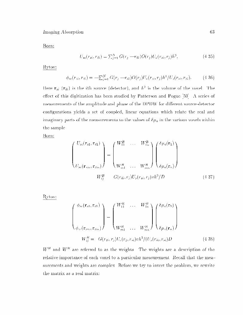
Imaging Absorption 63
Born:
Usc(rsi; rdi) =PN
j=1G(rj � rdi)O(rj)Uo(rsi; rj)h3; (4.35)
Rytov:
�sc(rsi; rdi) = �PN
j=1G(rj � rdi)O(rj)Uo(rsi; rj)h3=Uo(rsi; rdi): (4.36)
Here rsi (rdi) is the ith source (detector), and h3 is the volume of the voxel. The
e�ect of this digitization has been studied by Patterson and Pogue [50]. A series of
measurements of the amplitude and phase of the DPDW for di�erent source-detector
con�gurations yields a set of coupled, linear equations which relate the real and
imaginary parts of the measurements to the values of ��a in the various voxels within
the sample.
Born: 0BBBBB@
Usc(rs1; rd1)
...
Usc(rsm; rdm)
1CCCCCA =
0BBBBB@
WB11 : : : WB
1n
.... . .
...
WBm1
: : : WBmn
1CCCCCA
0BBBBB@
��a(r1)
...
��a(rn)
1CCCCCA
WBij = G(rdi; rj)Uo(rsi; rj)vh
3=D (4.37)
Rytov: 0BBBBB@
�sc(rs1; rd1)
...
�sc(rsm; rdm)
1CCCCCA =
0BBBBB@
WR11 : : : WR
1n
.... . .
...
WRm1 : : : WR
mn
1CCCCCA
0BBBBB@
��a(r1)
...
��a(rn)
1CCCCCA
WRij = G(rdi; rj)Uo(rj ; rsi)vh3=(Uo(rdi; rsi)D (4.38)
WB and WR are referred to as the weights. The weights are a description of the
relative importance of each voxel to a particular measurement. Recall that the mea-
surements and weights are complex. Before we try to invert the problem, we rewrite
the matrix as a real matrix;
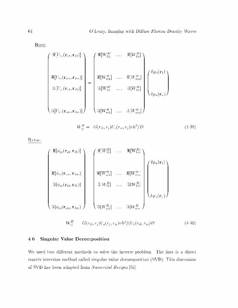
64 O'Leary, Imaging with Di�use Photon Density Waves
Born:
0BBBBBBBBBBBBBBBBBBBB@
<[Usc(rs1; rd1)]
...
<[Usc(rsm; rdm)]
=[Usc(rs1; rd1)]
...
=[Usc(rsm; rdm)]
1CCCCCCCCCCCCCCCCCCCCA
=
0BBBBBBBBBBBBBBBBBBBB@
<[WB11] : : : <[WB
1n]
.... . .
...
<[WBm1] : : : <[WB
mn]
=[WB11] : : : =[WB
1n]
.... . .
...
=[WBm1] : : : =[WB
mn]
1CCCCCCCCCCCCCCCCCCCCA
0BBBBB@
��a(r1)
...
��a(rn)
1CCCCCA
WBij = G(rdi; rj)Uo(rsi; rj)vh3=D (4.39)
Rytov:
0BBBBBBBBBBBBBBBBBBBB@
<[�sc(rs1; rd1)]
...
<[�sc(rsm; rdm)]
=[�sc(rs1; rd1)]
...
=[�sc(rsm; rdm)]
1CCCCCCCCCCCCCCCCCCCCA
=
0BBBBBBBBBBBBBBBBBBBB@
<[WR11] : : : <[WR
1n]
.... . .
...
<[WRm1] : : : <[WR
mn]
=[WR11] : : : =[WR
1n]
.... . .
...
=[WRm1] : : : =[WR
mn]
1CCCCCCCCCCCCCCCCCCCCA
0BBBBBBBBBB@
��a(r1)
...
��a(rn)
1CCCCCCCCCCA
WRij = G(rdi; rj)Uo(rj ; rsi)vh3=(Uo(rdi; rsi)D (4.40)
4.6 Singular Value Decomposition
We used two di�erent methods to solve the inverse problem. The �rst is a direct
matrix inversion method called singular value decomposition (SVD). This discussion
of SVD has been adapted from Numerical Recipes [51].
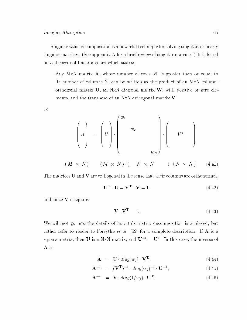
Imaging Absorption 65
Singular value decomposition is a powerful technique for solving singular, or nearly
singular matrices. (See appendix A for a brief review of singular matrices.) It is based
on a theorem of linear algebra which states:
Any MxN matrix A, whose number of rows M, is greater than or equal to
its number of columns N, can be written as the product of an MxN column-
orthogonal matrix U, an NxN diagonal matrix W, with positive or zero ele-
ments, and the transpose of an NxN orthogonal matrix V.
i.e.
0BBBBB@A
1CCCCCA =
0BBBBB@U
1CCCCCA �
0BBBBBBBBBB@
w1
w2
. . .
wN
1CCCCCCCCCCA�
0BBBBB@ V T
1CCCCCA
(M � N ) (M � N ) � ( N � N ) � (N � N ) (4.41)
The matricesU andV are orthogonal in the sense that their columns are orthonormal,
UT�U = VT
�V = 1: (4.42)
and since V is square,
V �VT = 1: (4.43)
We will not go into the details of how this matrix decomposition is achieved, but
rather refer to reader to Forsythe et al. [52] for a complete description. If A is a
square matrix, then U is a NxN matrix, and U�1 = UT . In this case, the inverse of
A is
A = U � diag(wj) �VT; (4.44)
A�1 = (VT)�1 � diag(wj)�1�U�1; (4.45)
A�1 = V � diag(1=wj) �UT: (4.46)
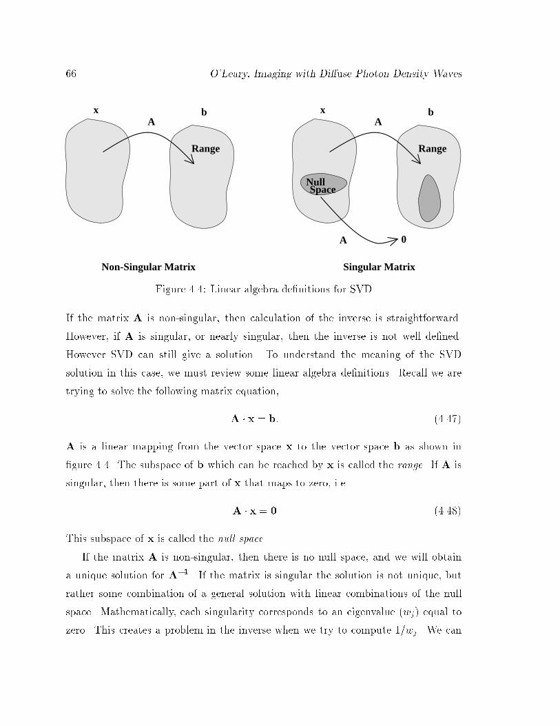
66 O'Leary, Imaging with Di�use Photon Density Waves
Non-Singular Matrix Singular Matrix
xA
b
Range
xA
b
0
Range
NullSpace
A
Figure 4.4: Linear algebra de�nitions for SVD
If the matrix A is non-singular, then calculation of the inverse is straightforward.
However, if A is singular, or nearly singular, then the inverse is not well de�ned.
However SVD can still give a solution. To understand the meaning of the SVD
solution in this case, we must review some linear algebra de�nitions. Recall we are
trying to solve the following matrix equation,
A � x = b: (4.47)
A is a linear mapping from the vector space x to the vector space b as shown in
�gure 4.4. The subspace of b which can be reached by x is called the range. If A is
singular, then there is some part of x that maps to zero, i.e.
A � x = 0 (4.48)
This subspace of x is called the null space.
If the matrix A is non-singular, then there is no null space, and we will obtain
a unique solution for A�1. If the matrix is singular the solution is not unique, but
rather some combination of a general solution with linear combinations of the null
space. Mathematically, each singularity corresponds to an eigenvalue (wj) equal to
zero. This creates a problem in the inverse when we try to compute 1/wj . We can
Imaging Absorption 67
however, generate the solution with the smallest absorption by setting 1/wj equal to
zero when wj equals zero. This is equivalent to throwing out all null space solutions.
This altering of the eigenvalues is called singular value analysis (SVA). One of the
powerful advantages of SVD is that the columns of V with zero eigenvalues form
a basis set for the null space. Thus we can easily check the solutions that we are
discarding for physical relevance.
The condition number of a matrix is the ratio of the smallest eigenvalue to the
largest. The closer to unity the condition number, the more robust the inversion. A
condition number of 10�6 for oating point precision of 10�12 for double precision
will result in eigenvalues which are dominated by round o� error. So SVA is also
needed when the range of the eigenvalues is larger that the numerical precision of the
computer. In the photon di�usion problem the condition number of the matrix is
typically 10�12. In this case we could zero the inverse of the small eigenvalues to gen-
erate the solution. We have found the that reconstructed images are improved when
we use a simple smoothing algorithm [53] instead of eliminating the small eigenvalues;
wj ! wj + �=wj (4.49)1
wj
!1
wj + �=wj
(4.50)
Figure 4.5 demonstrates how the eigenvalues are e�ected by such an algorithm. �
is an arbitrary free parameter. If � is much larger than the square of the maximum
eigenvalue, then the eigenvalues are dramatically reduced, and we obtain a solution
composed of only a few of the largest eigenfunctions. If � is small compared to
the square of the smallest eigenvalue, then there is e�ectively no smoothing, and we
obtain a solution dominated by noise. Although the norm of the solution is reduced
as we increase the smoothing, this is not the same as Tikhonov regularization where
we minimize the norm of the residual plus the norm of the solution. The advantage
of using the smoothing method over Tikhonov regularization is that we only have to
perform the time consuming matrix decomposition once.
We can now write down an explicit solution for the absorption as a function of

68 O'Leary, Imaging with Di�use Photon Density Waves
0
σ =
1e10σ =
1e05
σ = 1e15
σ = 1e10
σ =
σ = 1e05
1e20
σ = 0
σ =
σ = 1e20
1e15
σ =
Figure 4.5: A singular or numerically singular matrix will have eigenvalues wj whichare zero or below the numerical precision of the calculation. In this case, we apply aneigenvalue smoothing procedure to minimize the e�ect of the small eigenvalues. Theleft panel shows how the eigenvalues are altered when wj ! wj + �=wj for a series ofdi�erent values of �. The right panel shows how the inverse eigenvalue is a�ected.
position;
( ��a ) = [(V ) � ( diag( 1
wj+�=wj) ) � (UT )] � ( data ) (4.51)
As we increase �, the image becomes less noisy and the image appears smoother.
Since the smoothing algorithm always decreases the inverse of wj , the reconstructed
absorption will also decrease as the smoothing factor is increased.
There are many other regularization algorithms. In particular, Arridge et al. [19]
have tested discussed Tikhonov regulation and SVA within the framework of di�usion
imaging.
We have presented SVD for a square matrix. In our case, we often have many
more voxels of unknown absorption than we do measurements. This means that we
have more unknowns than equations. In this situation, we simply pad the matrix A
with rows of zeros, and likewise pad the measurement vector with zeros. We can then
invert the square matrix. The solution that we obtain will have a zero eigenvalue
for each row of padding, and the solution we get is approximately the minimum
Imaging Absorption 69
absorption solution as discussed above.
4.7 Algebraic Reconstruction Techniques
The second method we used to solve the linear system of equations is an algebraic
reconstruction technique called SIRT - simultaneous iterative reconstruction tech-
nique. SIRT is a slight modi�cation to an algebraic reconstruction technique (ART).
In this section we will describe ART, and then SIRT. This discussion is based on the
discussion in Kak et al. [48].
The ART algorithm is best demonstrated pictorially using a simple example. Sup-
pose we have a system with two linear equations and two unknowns,
~A � ~x = ~b (4.52)
A11x1 +A12x2 = b1 (4.53)
A21x1 +A22x2 = b2: (4.54)
Here b1 and b2 are measurements, x1 and x2 are unknowns, and the A's are calcu-
lable. The solution space is a 2 dimensional space, i.e. a plane spanned by x1 and
x2. The measurements are lines in that plane with slopes �A11=A12, �A21=A22 and
intercepts b1=A12; b2=A22 as shown in �gure 4.6a. The solution we are searching for is
the intersection of these two lines. To �nd the intersection using ART, we �rst start
from any point in space. (Typically we choose the origin as the initial guess.) We
then move from the origin to the closest point on line �rst line as shown in �gure 4.6.
The mathematical equation for the move is
~xnew = ~x�~x � ~A� bj~A � ~A
~A (4.55)
Here ~A = (Aj1; Aj2:::AjN) and ~x = (x1; x2) is the the initial guess. We next make a
similar move from the �rst line to the second line. These two moves constitute one
iteration. This process, called the Kaczmarz method, is repeated until convergence
is achieved. Tanube [54] has shown that the algorithm will always converge on the
correct solution if a unique solution exists.
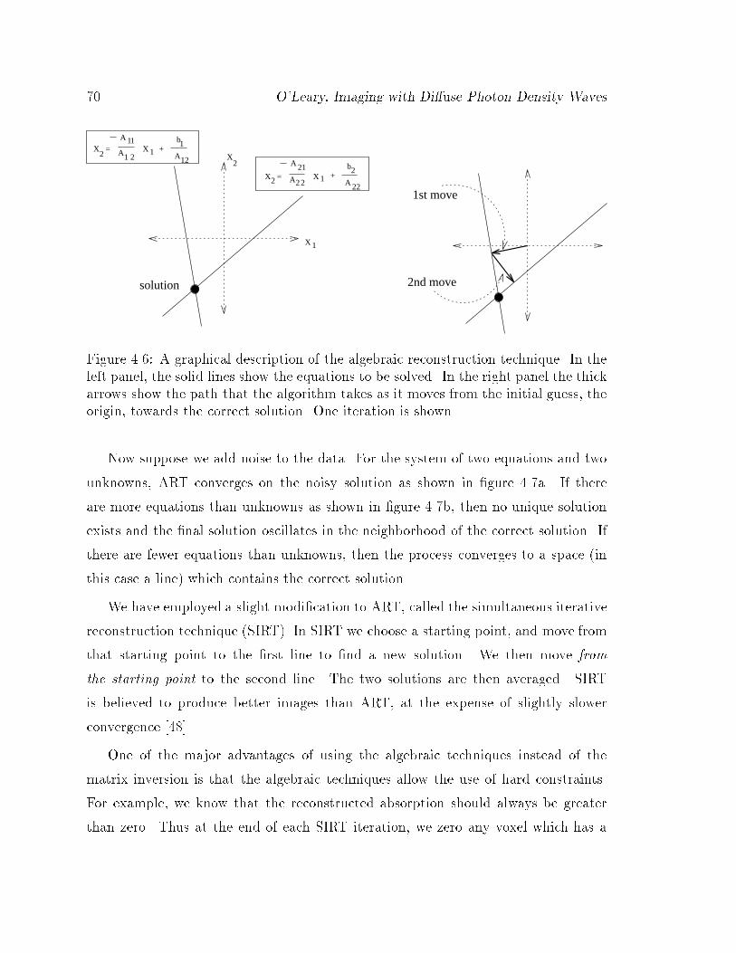
70 O'Leary, Imaging with Di�use Photon Density Waves
A 21
A22X 1 A 22
X = 2
X2
X 1
+A 1
A 2X 1
b
A 2X =
2
1
1
1
1
+b2
2nd move
1st move
solution
Figure 4.6: A graphical description of the algebraic reconstruction technique. In theleft panel, the solid lines show the equations to be solved. In the right panel the thickarrows show the path that the algorithm takes as it moves from the initial guess, theorigin, towards the correct solution. One iteration is shown.
Now suppose we add noise to the data. For the system of two equations and two
unknowns, ART converges on the noisy solution as shown in �gure 4.7a. If there
are more equations than unknowns as shown in �gure 4.7b, then no unique solution
exists and the �nal solution oscillates in the neighborhood of the correct solution. If
there are fewer equations than unknowns, then the process converges to a space (in
this case a line) which contains the correct solution.
We have employed a slight modi�cation to ART, called the simultaneous iterative
reconstruction technique (SIRT). In SIRT we choose a starting point, and move from
that starting point to the �rst line to �nd a new solution. We then move from
the starting point to the second line. The two solutions are then averaged. SIRT
is believed to produce better images than ART, at the expense of slightly slower
convergence [48].
One of the major advantages of using the algebraic techniques instead of the
matrix inversion is that the algebraic techniques allow the use of hard constraints.
For example, we know that the reconstructed absorption should always be greater
than zero. Thus at the end of each SIRT iteration, we zero any voxel which has a
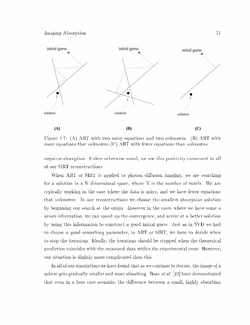
Imaging Absorption 71
solution
(A) (B) (C)
solution solution
initial guessinitial guessinitial guess
Figure 4.7: (A) ART with two noisy equations and two unknowns. (B) ART withmore equations that unknowns (C) ART with fewer equations than unknowns.
negative absorption. Unless otherwise noted, we use this positivity constraint in all
of our SIRT reconstructions.
When ART or SIRT is applied to photon di�usion imaging, we are searching
for a solution in a N dimensional space, where N is the number of voxels. We are
typically working in the case where the data is noisy, and we have fewer equations
that unknowns. In our reconstructions we choose the smallest absorption solution
by beginning our search at the origin. However in the cases where we have some a
priori information, we can speed up the convergence, and arrive at a better solution
by using this information to construct a good initial guess. Just as in SVD we had
to choose a good smoothing parameter, in ART or SIRT, we have to decide when
to stop the iterations. Ideally, the iterations should be stopped when the theoretical
prediction coincides with the measured data within the experimental error. However,
our situation is slightly more complicated than this.
In all of our simulations we have found that as we continue to iterate, the image of a
sphere gets gradually smaller and more absorbing. Boas et al. [22] have demonstrated
that even in a best case scenario, the di�erence between a small, highly absorbing
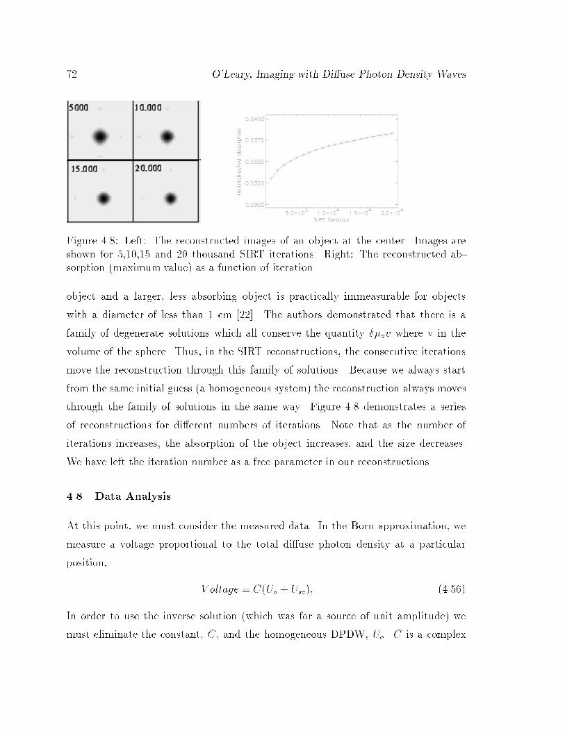
72 O'Leary, Imaging with Di�use Photon Density Waves
Figure 4.8: Left: The reconstructed images of an object at the center. Images areshown for 5,10,15 and 20 thousand SIRT iterations. Right: The reconstructed ab-sorption (maximum value) as a function of iteration.
object and a larger, less absorbing object is practically immeasurable for objects
with a diameter of less than 1 cm [22]. The authors demonstrated that there is a
family of degenerate solutions which all conserve the quantity ��av where v in the
volume of the sphere. Thus, in the SIRT reconstructions, the consecutive iterations
move the reconstruction through this family of solutions. Because we always start
from the same initial guess (a homogeneous system) the reconstruction always moves
through the family of solutions in the same way. Figure 4.8 demonstrates a series
of reconstructions for di�erent numbers of iterations. Note that as the number of
iterations increases, the absorption of the object increases, and the size decreases.
We have left the iteration number as a free parameter in our reconstructions.
4.8 Data Analysis
At this point, we must consider the measured data. In the Born approximation, we
measure a voltage proportional to the total di�use photon density at a particular
position,
V oltage = C(Uo + Usc); (4.56)
In order to use the inverse solution (which was for a source of unit amplitude) we
must eliminate the constant, C, and the homogeneous DPDW, Uo. C is a complex
Imaging Absorption 73
number which includes such factors as the signal ampli�cation, the e�ciency of the
light detection and the initial amplitude and phase of the source. In our experiments
we measure the amplitude and phase of C by making measurements in a homogeneous
in�nite medium.
After calculating C, we have to subtract o� the homogeneous part of the sig-
nal. This may be done using an analytic solution if the background properties are
known. Alternatively, researchers have measured the signal with and without the
presence on an inhomogeneity to eliminate the background. However, since both of
these measurements are impractical in a clinical situation, we have instead chosen to
make a reference measurement which does not rely on �nding a homogeneous portion
of the sample. In such a scheme we make two measurements with the same source
and detector separations as shown in �gure 4.9. We then subtract the two measure-
ments, eliminating the homogeneous signal, and are left with only the di�erence of
the heterogeneous signals.
V oltage 1� V oltage 2 = C(Uo + U1
sc) �C(Uo + U2
sc) (4.57)
= C(U1
sc � U2
sc:) (4.58)
Of course using pairs of measurements changes the form of the weights;
WBij = [G(rj � rdi1)Uo(rsi1; rj)�G(rj � rdi2)Uo(rsi2; rj)] vh
3=D: (4.59)
For the Rytov approximation, the situation is slightly simpler. In this case we
measure
V oltage = CUo exp(�sc) (4.60)
Again, we could measure or calculate C and Uo. However, if we use the reference
scheme discussed above, and this time divide the two measurements,
ln
V oltage 1
V oltage 2
!= ln
CUo exp(�sc1)
CUo exp(�sc2)
!= �sc1 � �sc2; (4.61)
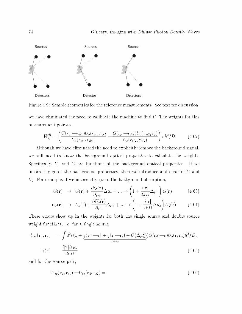
74 O'Leary, Imaging with Di�use Photon Density Waves
DetectorDetectors Detectors
SourcesSources Source
Figure 4.9: Sample geometries for the referencemeasurements. See text for discussion.
we have eliminated the need to calibrate the machine to �nd C. The weights for this
measurement pair are
WRij =
G(rj � rdi1)Uo(rsi1; rj)
Uo(rsi1; rdi1)�G(rj � rdi2)Uo(rsi2; rj)
Uo(rsi2; rdi2)
!vh3=D: (4.62)
Although we have eliminated the need to explicitly remove the background signal,
we still need to know the background optical properties to calculate the weights.
Speci�cally, Uo and G are functions of the background optical properties. If we
incorrectly guess the background properties, then we introduce and error in G and
Uo. For example, if we incorrectly guess the background absorption,
G(r) ! G(r) +@G(r)
@�a��a + :::!
1 +
ijrj
2kD��a
!G(r) (4.63)
Uo(r) ! Uo(r) +@Uo(r)
@�a��a + :::!
1 +
ijrj
2kD��a
!Uo(r) (4.64)
These errors show up in the weights for both the single source and double source
weight functions, i.e. for a single source
Usc(rd; rs) =Zd3r(1 + (rd � r) + (r� rs) +O(��2a)| {z }
error
)G(rd � r)Uo(r; rs)h3=D;
(r) =ijrj��a2kD
(4.65)
and for the source pair,
Usc(rd; rs1)� Usc(rd; rs2) = (4.66)
Imaging Absorption 75
Zd3r
264(1 + (rd � r) + (r� rs1) +O(��2a)| {z }
error
)G(rd � r)Uo(r; rs1)
�(1 + (rd � r) + (r� rs2) +O(��2a)| {z }error
)G(rd � r)Uo(r; rs2)
375h3=D
We can see that the same systematic error is introduced in each equation for incorrect
estimates of �a. If we now look at the calculation of Usc from the measured data, we
see the di�erence between the one source and two source measurements. When we
measure the amplitude and phase, we measure the total wave,
Utotal = Uo + Usc ! Usc = Utotal � Uo: (4.67)
In the one source Born approximation we must subtract o� the calculated value of
Uo. Since we use a guess for the background properties to calculate Uo, we introduce
some error here, i.e.
Usc(rs; rd) = Utotal(rs; rd)� (1 + (rs; rd))Uo(rs; rd): (4.68)
But when we use the two source referencing method, since jrd � rs1j = jrd � rs2j this
error is eliminated,
Usc(rs1; rd)� Usc(rs2; rd) = [Utotal(rs1; rd)� (1 � (rd; rs1))(Uo(rs1; rd)] (4.69)
� [Utotal(rs2; rd)� (1 � (rd; rs2))Uo(rs2; rd)]
= Utotal(rs1; rd)� Utotal(rs2; rd) (4.70)
There is no systematic error introduced in the measurement of Usc when using the
referencing scheme. Note that the if there is random measurement noise, then the
subtraction of the two source measurements will e�ectively double the random noise.
Only the error in the processed data is reduced by the referencing scheme, the
error in the weights is not reduced. Nevertheless, we have found that the proce-
dure gives superior reconstruction as shown in �gure 4.10. In these simulations, the
background medium has an absorption coe�cient of �a = 0:03 cm�1 and a reduced
76 O'Leary, Imaging with Di�use Photon Density Waves
scattering coe�cient of �0s = 10:0 cm�1. A 1 cm diameter sphere with the same
reduced scattering coe�cient as the background and an absorption coe�cient of 0:05
cm�1 is embedded in the medium. The source (or sources) are scanned around the
edges of a 7 cm square, and 26 measurements of amplitude and phase are simulated at
a source modulation frequency of 500 MHz. We use the analytic solution for a sphere
[10] to simulate the data. No noise was added to the data. We obtained data for two
di�erent con�gurations, �rst, a single source directly across from a single detector,
and second, a source pair separated by 1 cm, directly across from a single detector.
Before we began reconstructing the image, we took a guess at the background
absorption, (we assume that we know the correct reduced scattering coe�cient). For
the single source measurements, we use this guess to calculate the weights. We
also use the guess to analytically subtract o� the background signal from the total
measurement. When the guess for the background was too low, (top left images in
�gure 4.10) a noisy image with a large positive absorption region in the center, and
negative absorption region at the edges. When the background absorption is guessed
correctly, we obtain a good image (center left image in �gure 4.10), and when the
background absorption guess is too high, we obtain the opposite image we saw when
we under estimated the background absorption (lower left images in �gure 4.10).
When we use the source pair, and underestimate the background absorption, this
error cancels in the measured data, and the error is propagated only through the
weights. In this situation, we can still see the outline of the solution in each case (see
�gure 4.11, right column). Although the error in the weights has e�ected the image
quality, but it has not totally degraded the image.
When a positivity constraint is placed on the absorption solution (i.e. we set all
voxels with negative absorption equal to zero in the reconstruction algorithm), the
quality of the two source reconstructions is improved. The single source reconstruction
only works when have the correct guess for the background (see �gure 4.11).
If the geometry of the system does not allow these symmetric measurements,
this algorithm for background subtraction cannot be used. Instead, the background
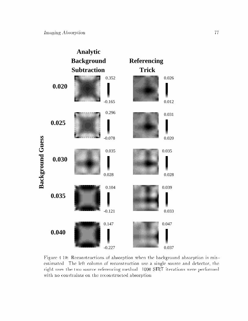
Imaging Absorption 77
0.040
0.035
0.030
0.025
0.020
BackgroundSubtraction
AnalyticReferencing
Trick
-0.165
-0.078
-0.121
-0.227
0.012
0.020
0.033
0.037
0.352
0.296
0.035
0.104
0.147
0.026
0.031
0.035
0.028
0.039
0.047
0.028
Bac
kgro
und
Gue
ss
Figure 4.10: Reconstructions of absorption when the background absorption is mis-estimated. The left column of reconstruction use a single source and detector, theright uses the two source referencing method. 1000 SIRT iterations were performedwith no constraints on the reconstructed absorption.
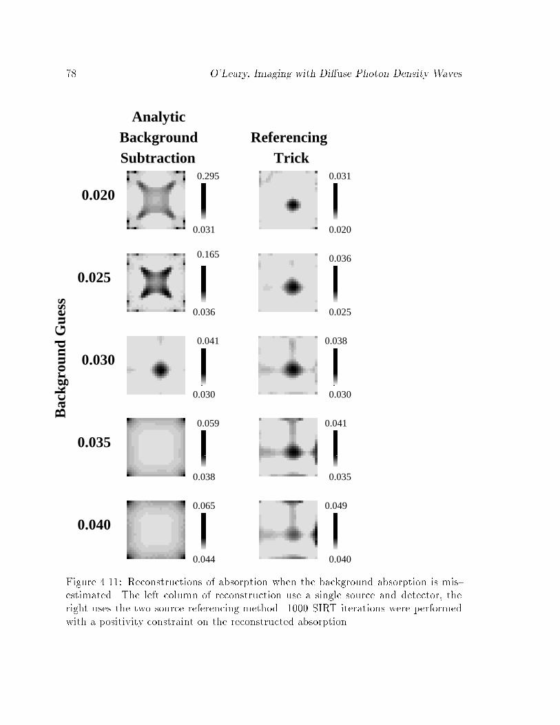
78 O'Leary, Imaging with Di�use Photon Density Waves
0.040
0.035
0.030
0.025
0.020
BackgroundSubtraction
AnalyticReferencing
Trick
0.031
0.036
0.030
0.038
0.044
0.020
0.025
0.030
0.035
0.040
0.295
0.165
0.041
0.059
0.065
0.031
0.036
0.038
0.041
0.049
Bac
kgro
und
Gue
ss
Figure 4.11: Reconstructions of absorption when the background absorption is mis-estimated. The left column of reconstruction use a single source and detector, theright uses the two source referencing method. 1000 SIRT iterations were performedwith a positivity constraint on the reconstructed absorption.
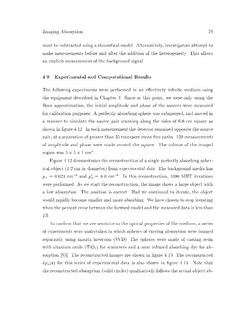
Imaging Absorption 79
must be subtracted using a theoretical model. Alternatively, investigators attempt to
make measurements before and after the addition of the heterogeneity. This allows
an explicit measurement of the background signal.
4.9 Experimental and Computational Results
The following experiments were performed in an e�ectively in�nite medium using
the equipment described in Chapter 3. Since at this point, we were only using the
Born approximation, the initial amplitude and phase of the sources were measured
for calibration purposes. A perfectly absorbing sphere was submerged, and moved in
a manner to simulate the source pair scanning along the sides of 6:0 cm square as
shown in �gure 4.12. In each measurement the detector remained opposite the source
pair, at a separation of greater than 35 transport mean free paths. 120 measurements
of amplitude and phase were made around the square. The volume of the imaged
region was 5 � 5 � 1 cm3.
Figure 4.12 demonstrates the reconstruction of a single perfectly absorbing spher-
ical object (1.2 cm in diameter) from experimental data. The background media has
�a = 0.023 cm�1 and �0s = 6.0 cm�1. In this reconstruction, 1000 SIRT iterations
were performed. As we start the reconstruction, the image shows a large object with
a low absorption. The position is correct. Had we continued to iterate, the object
would rapidly become smaller and more absorbing. We have chosen to stop iterating
when the percent error between the forward model and the measured data is less than
1%.
To con�rm that we are sensitive to the optical properties of the medium, a series
of experiments were undertaken in which spheres of varying absorption were imaged
separately using matrix inversion (SVD). The spheres were made of casting resin
with titanium oxide (TiO2) for scatterers and a near infrared absorbing dye for ab-
sorption [55]. The reconstructed images are shown in �gure 4.13. The reconstructed
��a(r) for this series of experimental data is also shown in �gure 4.13. Note that
the reconstructed absorption (solid circles) qualitatively follows the actual object ab-
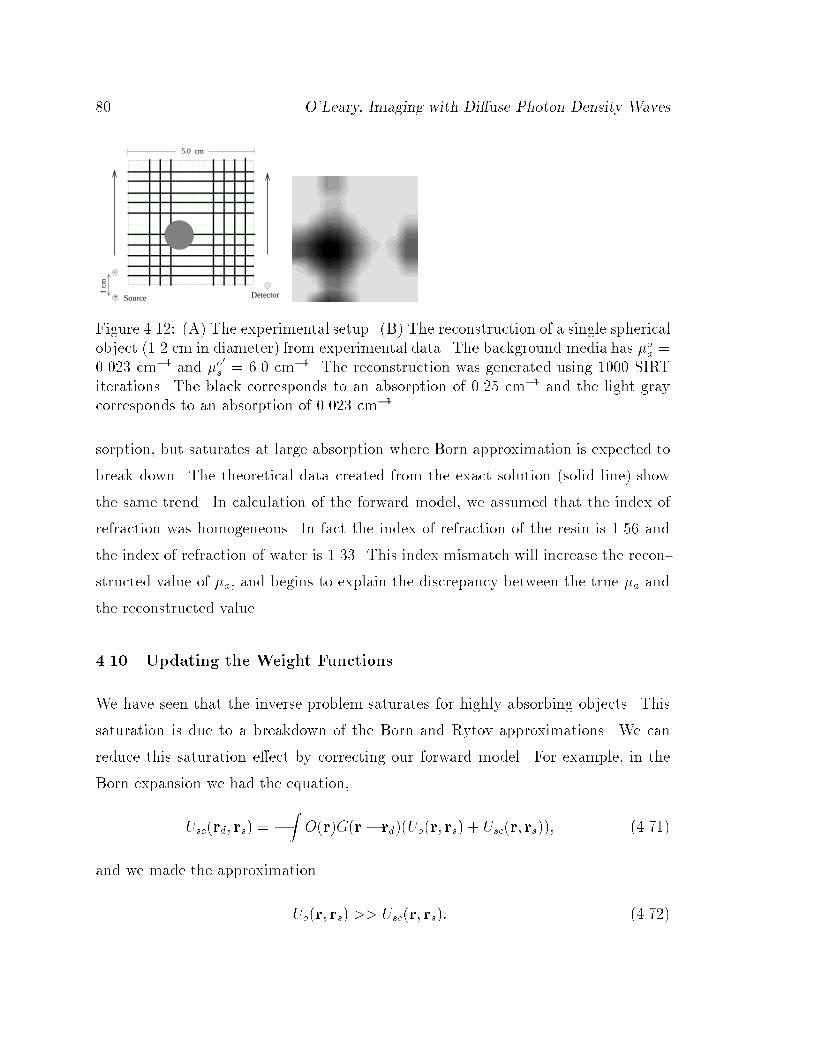
80 O'Leary, Imaging with Di�use Photon Density Waves
5.0 cm
1 cm
-
+ DetectorSource
Figure 4.12: (A) The experimental setup. (B) The reconstruction of a single sphericalobject (1.2 cm in diameter) from experimental data. The background media has �oa =0.023 cm�1 and �o
0
s = 6.0 cm�1. The reconstruction was generated using 1000 SIRTiterations. The black corresponds to an absorption of 0.25 cm�1 and the light graycorresponds to an absorption of 0.023 cm�1
sorption, but saturates at large absorption where Born approximation is expected to
break down. The theoretical data created from the exact solution (solid line) show
the same trend. In calculation of the forward model, we assumed that the index of
refraction was homogeneous. In fact the index of refraction of the resin is 1.56 and
the index of refraction of water is 1.33. This index mismatch will increase the recon-
structed value of �a, and begins to explain the discrepancy between the true �a and
the reconstructed value.
4.10 Updating the Weight Functions
We have seen that the inverse problem saturates for highly absorbing objects. This
saturation is due to a breakdown of the Born and Rytov approximations. We can
reduce this saturation e�ect by correcting our forward model. For example, in the
Born expansion we had the equation,
Usc(rd; rs) = �
ZO(r)G(r� rd)(Uo(r; rs) + Usc(r; rs)); (4.71)
and we made the approximation
Uo(r; rs) >> Usc(r; rs): (4.72)
Imaging Absorption 81
Figure 4.13: Top: In this experiment, resin spheres (1.2 cm diameter) made witha mixture of scatterer and a known concentration of ink were imaged using matrixinversion (SVD). Bottom: The reconstructed absorption from both the experimentaldata (circles) and the simulated data (line) are plotted vs the actual absorption. Seetext for further discussion. Error bars are derived from estimated the calibrationerrors which we believe to be most signi�cant.
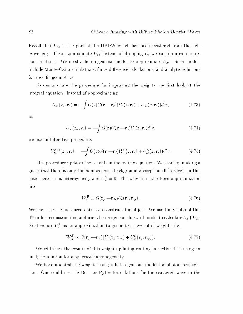
82 O'Leary, Imaging with Di�use Photon Density Waves
Recall that Usc is the part of the DPDW which has been scattered from the het-
erogeneity. If we approximate Usc instead of dropping it, we can improve our re-
constructions. We need a heterogeneous model to approximate Usc. Such models
include Monte-Carlo simulations, �nite di�erence calculations, and analytic solutions
for speci�c geometries.
To demonstrate the procedure for improving the weights, we �rst look at the
integral equation. Instead of approximating
Usc(rd; rs) = �
ZO(r)G(r � rd)(Uo(r; rs) + Usc(r; rs))d
3r; (4.73)
as
Usc(rd; rs) = �
ZO(r)G(r � rd)Uo(r; rs)d
3r; (4.74)
we use and iterative procedure,
Un+1sc (rd; rs) = �
ZO(r)G(r � rd)(Uo(r; rs) + Un
sc(r; rs))d3r: (4.75)
This procedure updates the weights in the matrix equation. We start by making a
guess that there is only the homogeneous background absorption (0th order). In this
case there is not heterogeneity and U0
sc = 0. The weights in the Born approximation
are
WBij / G(rj � rdi)Uo(rj; rsj): (4.76)
We then use the measured data to reconstruct the object. We use the results of this
0th order reconstruction, and use a heterogeneous forward model to calculate Uo+U1
sc.
Next we use U1
sc as an approximation to generate a new set of weights, i.e.,
WBij / G(rj � rdi)(Uo(rj; rsj) + U1
sc(rj; rsj)): (4.77)
We will show the results of this weight updating routing in section 4.12 using an
analytic solution for a spherical inhomogeneity.
We have updated the weights using a heterogeneous model for photon propaga-
tion. One could use the Born or Rytov formulations for the scattered wave in the
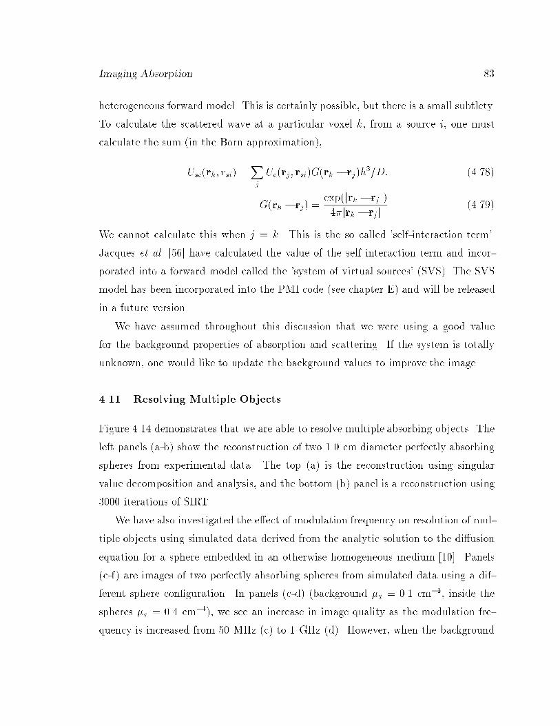
Imaging Absorption 83
heterogeneous forward model. This is certainly possible, but there is a small subtlety.
To calculate the scattered wave at a particular voxel k, from a source i, one must
calculate the sum (in the Born approximation),
Usc(rk; rsi) =Xj
Uo(rj; rsi)G(rk � rj)h3=D: (4.78)
G(rk � rj) =exp(jrk � rj j)
4�jrk � rjj(4.79)
We cannot calculate this when j = k. This is the so called 'self-interaction term'.
Jacques et al. [56] have calculated the value of the self interaction term and incor-
porated into a forward model called the 'system of virtual sources' (SVS). The SVS
model has been incorporated into the PMI code (see chapter E) and will be released
in a future version.
We have assumed throughout this discussion that we were using a good value
for the background properties of absorption and scattering. If the system is totally
unknown, one would like to update the background values to improve the image.
4.11 Resolving Multiple Objects
Figure 4.14 demonstrates that we are able to resolve multiple absorbing objects. The
left panels (a-b) show the reconstruction of two 1.0 cm diameter perfectly absorbing
spheres from experimental data. The top (a) is the reconstruction using singular
value decomposition and analysis, and the bottom (b) panel is a reconstruction using
3000 iterations of SIRT.
We have also investigated the e�ect of modulation frequency on resolution of mul-
tiple objects using simulated data derived from the analytic solution to the di�usion
equation for a sphere embedded in an otherwise homogeneous medium [10]. Panels
(c-f) are images of two perfectly absorbing spheres from simulated data using a dif-
ferent sphere con�guration. In panels (c-d) (background �a = 0.1 cm�1, inside the
spheres �a = 0.4 cm�1), we see an increase in image quality as the modulation fre-
quency is increased from 50 MHz (c) to 1 GHz (d). However, when the background
84 O'Leary, Imaging with Di�use Photon Density Waves
absorption is high (background �a = 1.0 cm�1, inside the spheres �a = 4.0 cm�1), the
image quality does not noticeably improve as the modulation frequency is increased
from 50 MHz (e) to 1 GHz (f). This may be understood qualitatively by noting that
the wavenumber of a DPDW,
k =q(�v�a + i!)=D; (4.80)
is nearly independent of ! when v�a >> !. This result suggests that sources at
low modulation frequencies and sources with high frequency components will yield
roughly equivalent images in media characterized by a high average absorption such
as the brain. On the other hand, when imaging within bodies with low average
absorption, such as the breast, high modulation frequency images will give better
resolution.
4.12 DPDW Imaging Combined With Other Imaging Modalities
An important contribution of the optical method is its ability to quantify the concen-
trations of physiologically important pigments, such as oxygenated and de-oxygenated
hemoglobin, by providing absolute spatial quanti�cation of scattering and absorption
coe�cients in the near infra-red region. Anatomical details derived from a conven-
tional medical image, as in the case of X-ray tomography or MRI, can be taken into
account in order to improve the quantitative accuracy of the optical image. The feasi-
bility of simultaneously combining optical with other imaging modalities promises to
increase the diagnostic certainty of the acquired images. Other researchers have used
a priori structural information to improve the formulation of the forward problem
[57, 58]. In this section we describe an algorithm which uses structural information
to reduce the number of unknowns in the inverse problem, from the number of voxels
in the image, to the number of tissue types. This reduces both the complexity of the
inverse problem and the number of measurements necessary for an accurate recon-
struction. We present simulations which con�rm the e�ciency of the algorithm, and
experimental measurements on a tissue phantom which demonstrate the feasibility of

Imaging Absorption 85
f)
c)
Experimental Datae)
Simulated Data
b)
a)
d)
Figure 4.14: The left panels (a-b) show the reconstruction of two 1.0 cm diameterperfectly absorbing spheres from experimental data. The top (a) is the reconstruc-tion using singular value decomposition and analysis, and the bottom (b) panel is areconstruction using 3000 iterations of SIRT. Panels (c-f) are images of two perfectlyspheres from simulated data using a di�erent sphere con�guration. In panels (c-d)(background �a = 0.1 cm�1, inside the spheres �a = 0.4 cm�1), we see an increase inimage quality as the modulation frequency is increased from 50 MHz (c) to 1 GHz(d). However, when the background absorption is high (background �a = 1.0 cm�1,inside the spheres �a = 4.0 cm�1) the image quality does not noticeably improve asthe modulation frequency is increased from 50 MHz (e) to 1 GHz (f).
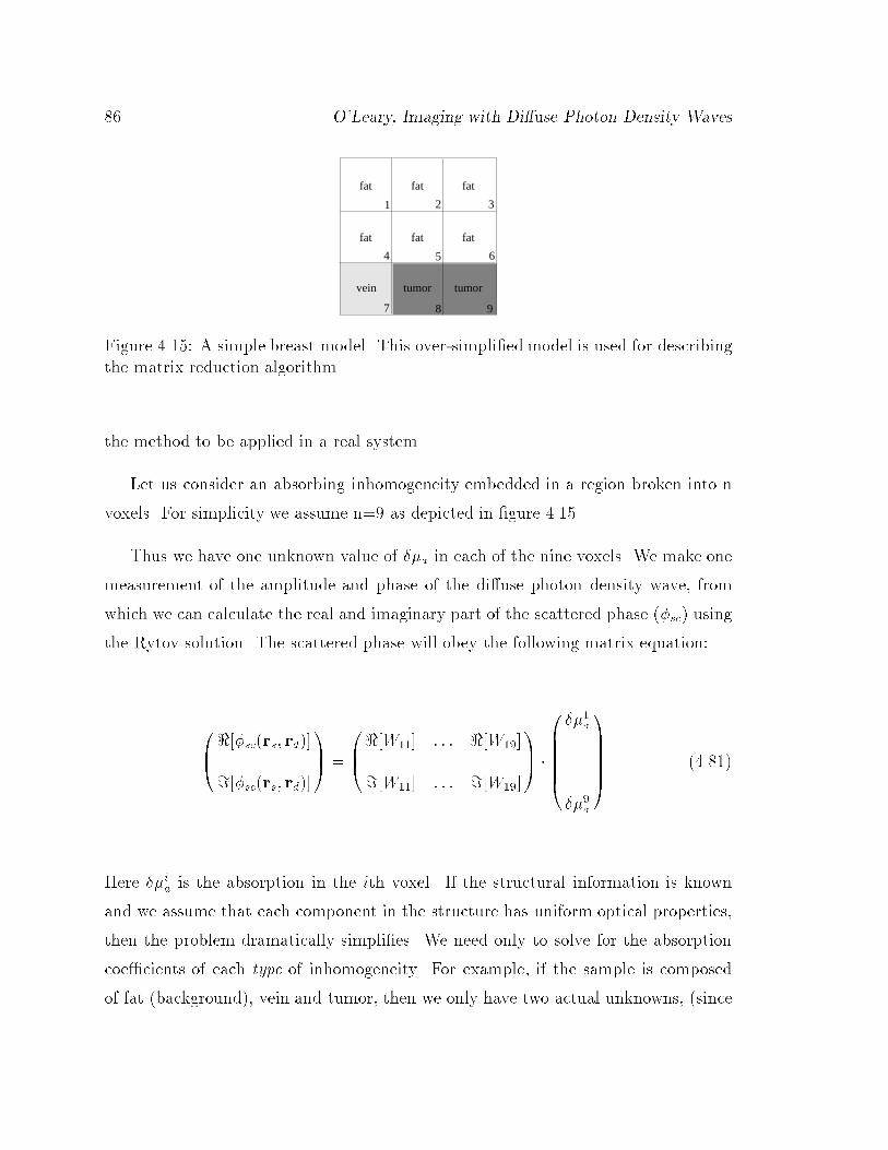
86 O'Leary, Imaging with Di�use Photon Density Waves
fat fat fat
fat fat fat
1 2 3
4 5 6
7 8 9
tumor tumorvein
Figure 4.15: A simple breast model. This over-simpli�ed model is used for describingthe matrix reduction algorithm.
the method to be applied in a real system.
Let us consider an absorbing inhomogeneity embedded in a region broken into n
voxels. For simplicity we assume n=9 as depicted in �gure 4.15.
Thus we have one unknown value of ��a in each of the nine voxels. We make one
measurement of the amplitude and phase of the di�use photon density wave, from
which we can calculate the real and imaginary part of the scattered phase (�sc) using
the Rytov solution. The scattered phase will obey the following matrix equation:
0B@<[�sc(rs; rd)]=[�sc(rs; rd)]
1CA =
0B@<[W11] : : : <[W19]
=[W11] : : : =[W19]
1CA �
0BBBBB@
��1a
...
��9a
1CCCCCA (4.81)
Here ��ia is the absorption in the ith voxel. If the structural information is known
and we assume that each component in the structure has uniform optical properties,
then the problem dramatically simpli�es. We need only to solve for the absorption
coe�cients of each type of inhomogeneity. For example, if the sample is composed
of fat (background), vein and tumor, then we only have two actual unknowns, (since
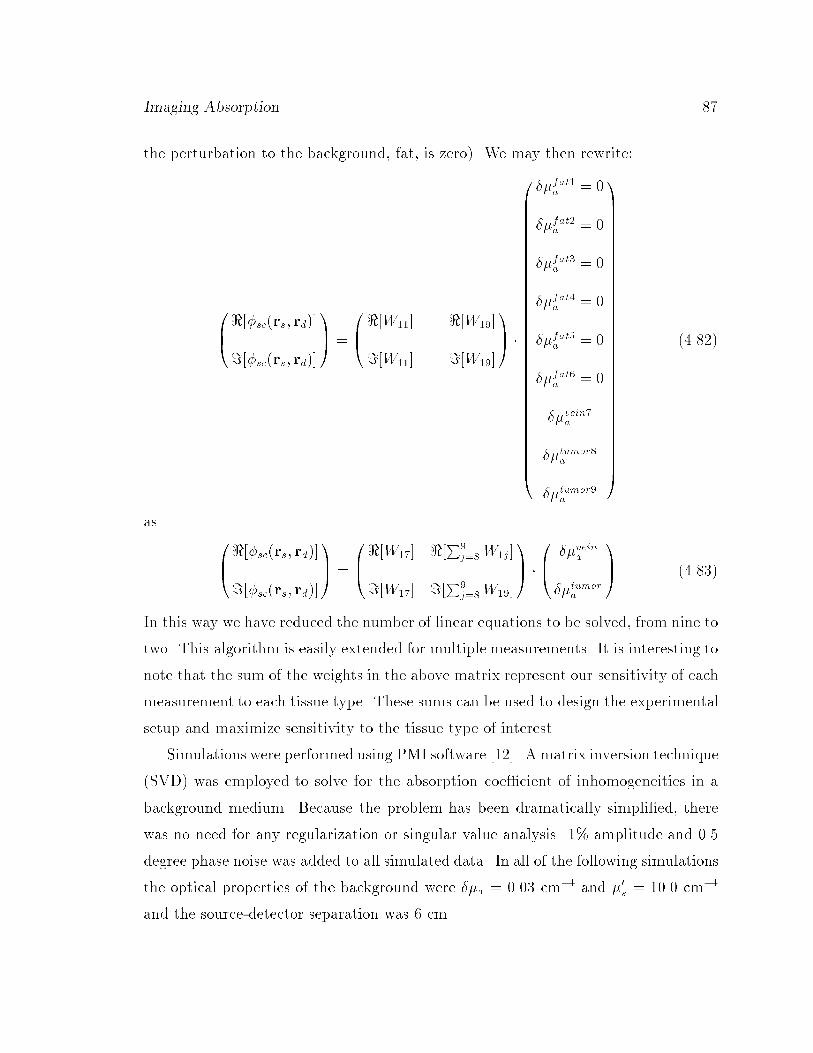
Imaging Absorption 87
the perturbation to the background, fat, is zero). We may then rewrite:
0B@<[�sc(rs; rd)]=[�sc(rs; rd)]
1CA =
0B@<[W11]
... <[W19]
=[W11]... =[W19]
1CA �
0BBBBBBBBBBBBBBBBBBBBBBBBBBBBBBBBBB@
��fat1a = 0
��fat2a = 0
��fat3a = 0
��fat4a = 0
��fat5a = 0
��fat6a = 0
��vein7a
��tumor8a
��tumor9a
1CCCCCCCCCCCCCCCCCCCCCCCCCCCCCCCCCCA
(4.82)
as 0B@<[�sc(rs; rd)]=[�sc(rs; rd)]
1CA =
0B@<[W17] <[
P9
j=8W1j]
=[W17] =[P
9
j=8W19]
1CA �
0B@ ��veina
��tumora
1CA (4.83)
In this way we have reduced the number of linear equations to be solved, from nine to
two. This algorithm is easily extended for multiple measurements. It is interesting to
note that the sum of the weights in the above matrix represent our sensitivity of each
measurement to each tissue type. These sums can be used to design the experimental
setup and maximize sensitivity to the tissue type of interest.
Simulations were performed using PMI software [12]. A matrix inversion technique
(SVD) was employed to solve for the absorption coe�cient of inhomogeneities in a
background medium. Because the problem has been dramatically simpli�ed, there
was no need for any regularization or singular value analysis. 1% amplitude and 0.5
degree phase noise was added to all simulated data. In all of the following simulations
the optical properties of the background were ��a = 0.03 cm�1 and �0s = 10.0 cm�1
and the source-detector separation was 6 cm.

88 O'Leary, Imaging with Di�use Photon Density Waves
We �rst tested this algorithm on a series of simple one object systems. The 1 cm
diameter spheres had the same scattering properties as the surrounding medium, but
the absorption varied from 0.035 to 0.355 cm�1. The area of interest, a 6 cm x 6
cm x 1 cm region, was divided into 120 x 120 x 20 = 288,000 voxels. Using a single
source-detector pair and making measurements of amplitude and phase at 4 di�erent
source modulation frequencies (50, 200, 350, 500 Mhz), we had a 8 x 288,000 matrix
to invert. But using the a priori structural information we were able to compress the
8 x 288,000 matrix down to a 8 x 1 matrix. In this reconstruction the computation
time was totally dominated by the time it takes to calculate the weights, and the
matrix inversion time was negligible. In �gure 4.16 the reconstructed value of the
object absorption is plotted versus the true value for each sphere simulation (labeled
1st iteration). Note that the reconstructed values agree well at low absorption, but
show saturation e�ects at higher absorption.
As we mentioned earlier, these saturation e�ects are a result of the breakdown of
the Rytov approximation. Basically, we have used a homogeneous model to calculate
the weight functions. To improve the reconstructions, we must take into account that
there is a heterogeneity present. When we updated the weight functions using the
1st iteration results, as suggested by Pogue et al. [20], we were able to overcome the
saturation e�ects. The imaging process now consists of several steps;
1. Create the weights using a homogeneous model.
2. Calculate the inverse using SVD.
3. Use this solution to calculate the weights using a heterogeneous model.
4. Calculate the inverse using SVD.
We have used the exact solution for a sphere to calculate the heterogeneous
weights. The results of this iterative process are also shown in 4.16, labeled 2nd
iteration.
The next simulation used six objects in the medium (background) as shown in
Fig. 3. Objects a,b,c,d had �a =0.036 cm�1, object e had �a =0.042 cm-1 and object
f had �a =0.050 cm�1. A single source and detector were scanned along the sides of
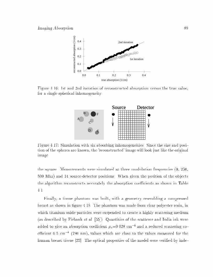
Imaging Absorption 89
0.0 0.1 0.2 0.3 0.4
0.0
0.1
0.2
0.3
0.4
reco
nstr
ucte
d ab
sorp
tion
(1/c
m)
true absorption (1/cm)
2nd iteration
1st iteration
Figure 4.16: 1st and 2nd iteration of reconstructed absorption versus the true value,for a single spherical inhomogeneity.
Source DetectorSource Detector
C
D E
FA
B
Figure 4.17: Simulation with six absorbing inhomogeneities. Since the size and posi-tion of the spheres are known, the 'reconstructed' image will look just like the originalimage.
the square. Measurements were simulated at three modulation frequencies (0, 250,
500 Mhz) and 14 source-detector positions. When given the position of the objects
the algorithm reconstructs accurately the absorption coe�cients as shown in Table
4.1.
Finally, a tissue phantom was built, with a geometry resembling a compressed
breast as shown in �gure 4.18. The phantom was made from clear polyester resin, in
which titanium oxide particles were suspended to create a highly scattering medium
(as described by Firbank et al. [55]). Quantities of the scatterer and India ink were
added to give an absorption coe�cient �a=0.028 cm�1 and a reduced scattering co-
e�cient 6.5 cm�1 (780 nm), values which are close to the values measured for the
human breast tissue [22]. The optical properties of the model were veri�ed by inde-
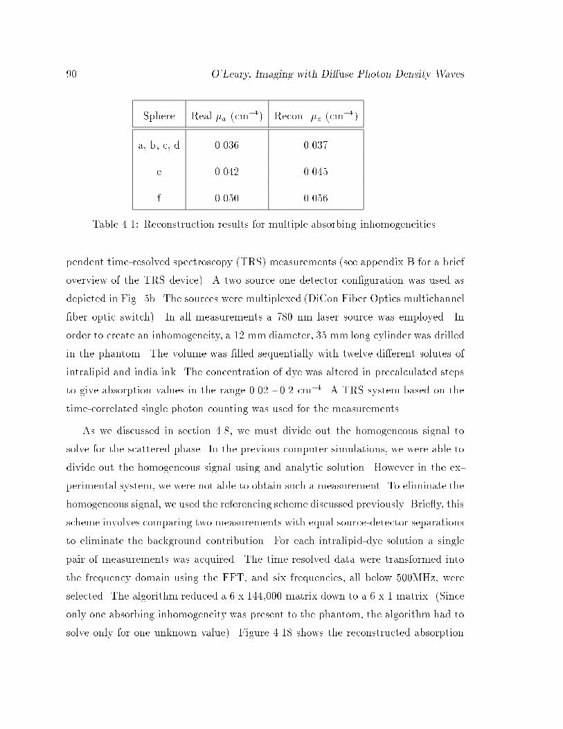
90 O'Leary, Imaging with Di�use Photon Density Waves
Sphere Real �a (cm�1) Recon. �a (cm
�1)
a, b, c, d 0.036 0.037
e 0.042 0.045
f 0.050 0.056
Table 4.1: Reconstruction results for multiple absorbing inhomogeneities.
pendent time-resolved spectroscopy (TRS) measurements (see appendix B for a brief
overview of the TRS device). A two source one detector con�guration was used as
depicted in Fig. 5b. The sources were multiplexed (DiCon Fiber Optics multichannel
�ber optic switch). In all measurements a 780 nm laser source was employed. In
order to create an inhomogeneity, a 12 mm diameter, 35 mm long cylinder was drilled
in the phantom. The volume was �lled sequentially with twelve di�erent solutes of
intralipid and india ink. The concentration of dye was altered in precalculated steps
to give absorption values in the range 0.02 - 0.2 cm�1. A TRS system based on the
time-correlated single photon counting was used for the measurements.
As we discussed in section 4.8, we must divide out the homogeneous signal to
solve for the scattered phase. In the previous computer simulations, we were able to
divide out the homogeneous signal using and analytic solution. However in the ex-
perimental system, we were not able to obtain such a measurement. To eliminate the
homogeneous signal, we used the referencing scheme discussed previously. Brie y, this
scheme involves comparing two measurements with equal source-detector separations
to eliminate the background contribution. For each intralipid-dye solution a single
pair of measurements was acquired. The time resolved data were transformed into
the frequency domain using the FFT, and six frequencies, all below 500MHz, were
selected. The algorithm reduced a 6 x 144,000 matrix down to a 6 x 1 matrix. (Since
only one absorbing inhomogeneity was present to the phantom, the algorithm had to
solve only for one unknown value). Figure 4.18 shows the reconstructed absorption
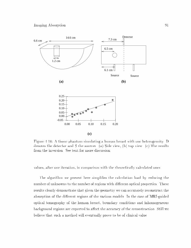
Imaging Absorption 91
-0.050.000.05
0.100.150.20
0.25
0.200.150.100.050.00
(b)(a)
14.6 cm7.3 cm
6.5 cm
6.1 cm
1.2 cm
6.6 cmDetector
SourceSource
(c)
Figure 4.18: A tissue phantom simulating a human breast with one heterogeneity. Ddenotes the detector and S the sources. (a) Side view, (b) top view. (c) The resultsfrom the inversion. See text for more discussion.
values, after one iteration, in comparison with the theoretically calculated ones.
The algorithm we present here simpli�es the calculation load by reducing the
number of unknowns to the number of regions with di�erent optical properties. These
results clearly demonstrate that given the geometry we can accurately reconstruct the
absorption of the di�erent regions of the various models. In the case of MRI-guided
optical tomography of the human breast, boundary conditions and inhomogeneous
background regions are expected to a�ect the accuracy of the reconstruction. Still we
believe that such a method will eventually prove to be of clinical value.
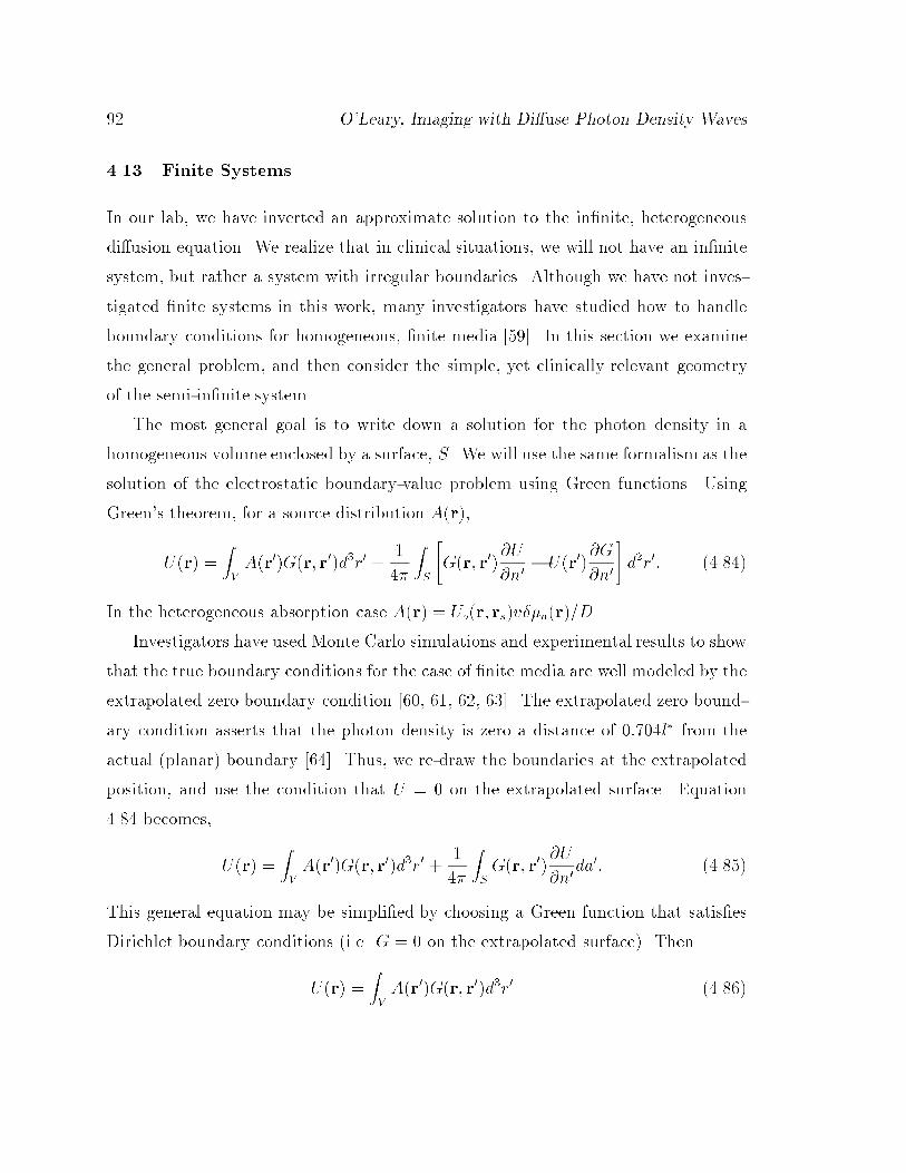
92 O'Leary, Imaging with Di�use Photon Density Waves
4.13 Finite Systems
In our lab, we have inverted an approximate solution to the in�nite, heterogeneous
di�usion equation. We realize that in clinical situations, we will not have an in�nite
system, but rather a system with irregular boundaries. Although we have not inves-
tigated �nite systems in this work, many investigators have studied how to handle
boundary conditions for homogeneous, �nite media [59]. In this section we examine
the general problem, and then consider the simple, yet clinically relevant geometry
of the semi-in�nite system.
The most general goal is to write down a solution for the photon density in a
homogeneous volume enclosed by a surface, S. We will use the same formalism as the
solution of the electrostatic boundary-value problem using Green functions. Using
Green's theorem, for a source distribution A(r),
U(r) =ZVA(r0)G(r; r0)d3r0 +
1
4�
ZS
"G(r; r0)
@U
@n0� U(r0)
@G
@n0
#d2r0: (4.84)
In the heterogeneous absorption case A(r) = Uo(r; rs)v��a(r)=D.
Investigators have used Monte Carlo simulations and experimental results to show
that the true boundary conditions for the case of �nite media are well modeled by the
extrapolated zero boundary condition [60, 61, 62, 63]. The extrapolated zero bound-
ary condition asserts that the photon density is zero a distance of 0:704l� from the
actual (planar) boundary [64]. Thus, we re-draw the boundaries at the extrapolated
position, and use the condition that U = 0 on the extrapolated surface. Equation
4.84 becomes,
U(r) =ZVA(r0)G(r; r0)d3r0 +
1
4�
ZSG(r; r0)
@U
@n0da0: (4.85)
This general equation may be simpli�ed by choosing a Green function that satis�es
Dirichlet boundary conditions (i.e. G = 0 on the extrapolated surface). Then
U(r) =ZVA(r0)G(r; r0)d3r0 (4.86)
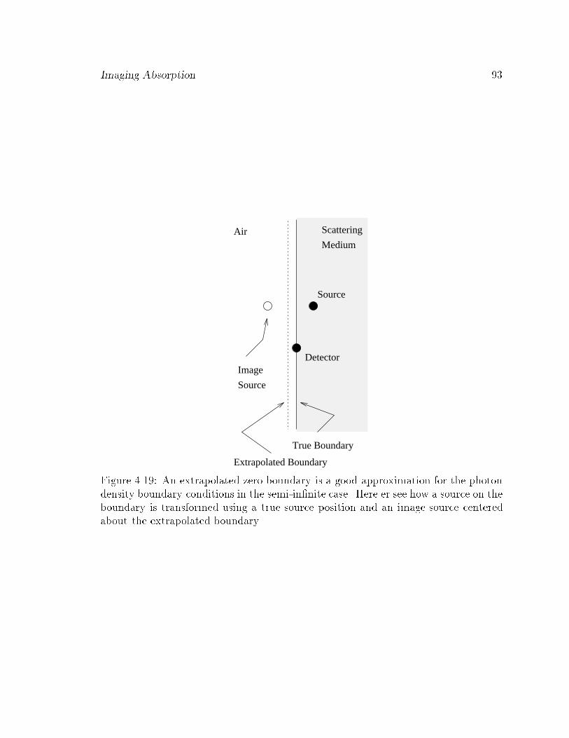
Imaging Absorption 93
Medium
Scattering
Extrapolated Boundary
True Boundary
Detector
Air
Source
Image
Source
Figure 4.19: An extrapolated zero boundary is a good approximation for the photondensity boundary conditions in the semi-in�nite case. Here er see how a source on theboundary is transformed using a true source position and an image source centeredabout the extrapolated boundary.
94 O'Leary, Imaging with Di�use Photon Density Waves
Arridge et al. [59] have worked out the Green function solutions for Dirichlet
boundary conditions for a variety of di�erent homogeneous �nite systems such as
semi-in�nite, slab, spherical and cylindrical geometries. It is also possible to use
other methods such as Monte-Carlo and Finite Element to derive the Green function
solutions.
For the semi-in�nite case, we can use the method of images to �nd the Green
function which obeys the Dirichlet boundary conditions (see �gure 4.19). In this case
G(r; r0) =exp(ikjr� r0j)
4�jr� r0j�exp(ikjr� rij)
4�jr� rij(4.87)
where r0 is the position of the source in the sample volume, and ri is the position of
the image source located on the other side of the extrapolated boundary. Using this
Green function we can now calculate the incident DPDW,
U(r; rs) =B
D
exp(ikjr� rsj)
4�jr� rsj�B
D
exp(ikjr� rij)
4�jr� rij(4.88)
= Uo(r; rs)� Uo(r; ri): (4.89)
where rs is the position of the source in the sample volume, and ri is the image of rs.
We now plug the incident DPDW solution and the Green Function solution for
the �nite system into the weights (equation 4.13,4.26). For example, in the Born
approximation, for a detector at rd, equation 4.13 becomes
Usc(rd; rs; ri) = �
Zd3r G(rd � r)| {z }
semi�infinite
O(r) Uo(r; rs)| {z }semi�infinite
(4.90)
= �
Zd3r [G(rd; r)�G(rd; r
0)] (4.91)
�O(r) [Uo(r; rs)� Uo(r; ri)]
where r0 is the image voxel position.
Multiple image sources can be used to solve for the scattered wave in the case of
the slab, the cube and other planar geometries. For curved geometries one has to
take more care in de�ning the extrapolated surface.
Chapter 5
Imaging the Scattering coe�cient
In the human body there are localized absorption changes and changes in the reduced
scattering coe�cient. Scattering is caused by a mismatch in the index of refraction
and depends on the size and shape of the scattering object. The reduced scattering
coe�cient also depends on the density of scatterers The presence of certain solutes
such as glucose or potassium can change the index of refraction of the intra- or extra-
cellular uid, changing the reduced scattering coe�cient. Imaging the scattering
coe�cient is important not only because large scattering changes can easily corrupt
an absorption image, but also because scattering is an additional form of contrast.
We will use the same expansions (Born, Rytov) that we used for the absorption
case and the same inversion techniques (SVD, SIRT) to image the reduced scattering
coe�cient.
To solve the di�usion equation for an in�nite, heterogeneously scattering medium
we expand the di�usion coe�cient, D = 1=3�0s, into spatially dependent, �D(r), and
independent (background), Do, pieces, i.e.
D(r)) �D(r) +Do: (5.1)
These terms are then incorporated into the di�usion equation (equation 2.18),
Jac(r) � �DrUac(r) (5.2)
to obtain
� i!U(r; rs) + v�aU(r; rs) +r � J(r; rs) = B�(rs); (5.3)
95
96 O'Leary, Imaging with Di�use Photon Density Waves
J(r; rs) = �(�D(r) +Do)rU(r; rs): (5.4)
When we insert equation 5.4 into 5.3, we obtain
� i!U(r; rs) + v�aU(r; rs)�r � ((�D(r) +Do)rU(r; rs)) = B�(rs): (5.5)
Then divide through by �Do we have
(r2 + k2)U(r; rs) +rF (r) � rU(r; rs) + F (r)r2U(r; rs) = �B�(rs)=Do (5.6)
F (r) = �D(r)=Do: (5.7)
5.1 Born Expansion
To solve this heterogeneous di�usion equation, we will use the same approaches as we
described in Chapter 4. We will assume that we have a homogeneous system. A �nite
system can be handled using image sources, just as we discussed in the absorption
case. First, using the Born approximation,
U(r; rs) = Uo(r; rs) + Usc(r; rs) (5.8)
so
(r2 + k2)Uo(r; rs)| {z }homogeneous
+(r2 + k2)Usc(r; rs) (5.9)
+rF (r) � r (Uo(r; rs) + Usc (r; rs)) + F (r)r2(Uo(r; rs) + Usc(r; rs))
= �B�(rs)=Do| {z }homogeneous
: (5.10)
If we subtract o� the homogeneous di�usion equation (marked homogeneous) and
assume that Usc � Uo, we again arrive at a Helmholtz equation for Usc,
(r2 + k2)Usc(r; rs) = �rF (r) � rUo(r; rs)� F (r)r2Uo(r; rs) (5.11)
which can be solved using the Green function method,
Usc(rd; rs) = �
Zd3r G(r � rd)
�rF (r) � rUo(r; rs) + F (r)r2 (Uo(r; rs))
�(5.12)
G(r� rd) =exp(jr� rdj)
4�jr� rdj: (5.13)
Imaging Scattering 97
Using Green's �rst identity [65],ZVd3x �r2 =
ZSd2x �n � r �
ZVd3x r� � r ; (5.14)
equation 5.12 becomes,
Usc(rd; rs) = �
ZVdr G(r� rd)rF (r) � rUo(r; rs)| {z }
I
(5.15)
�
ZSda Uo(r; rs)n � r (G(r � rd)F (r))| {z }
II
+ZVdr rUo(r; rs) � r (G(r � rd)F (r))| {z }
III
:
The integral marked II is equal to zero, since we can take this surface to be at in�nity,
and both Uo and G exponentially decay to zero at in�nity. The third integral can be
expanded,ZVdr rUo(r; rs) � r (G(r � rd)F (r)) =
ZVdr rUo(r; rs) � rG(r� rd)F (r)
+ZVdr rUo(r; rs) � rF (r)G(r� rd): (5.16)
Note that the second term in the expansion cancels with the termmarked I in equation
5.15 and �nally
Usc(rd; rs) =ZVdr rUo(r; rs) � rG(r� rd)
�D(r)
Do
: (5.17)
5.2 Rytov Expansion
Just as we did in the absorption case, we can also make a Rytov approximation,
U(r; rs) = Uo(r; rs)Usc(r; rsc) = exp(�o(r; rs) + �sc(r; rs)); (5.18)
Uo(r; rs) = exp(�o(r; rs)): (5.19)
For notational ease we will de�ne,
Uo � Uo(r; rs);�o � �o(r; rs) (5.20)
Usc � Usc(r; rs);�sc � �sc(r; rs): (5.21)
98 O'Leary, Imaging with Di�use Photon Density Waves
When we plug these terms into the di�usion equation (5.6) we arrive at,
(r2 + k2)(UoUsc) +rF � r(UoUsc) + Fr2(UoUsc) = �B�(rs)=Do (5.22)
F = �D(r)=Do: (5.23)
We can expand the gradients of products,
r2UoUsc +r
2UscUo + 2rUo � rUsc + k2UoUsc +rF � rUoUsc (5.24)
+rF � rUscUo + Fr2UoUsc + Fr2UscUo + 2FrUo � rUsc = �B�(rs)=Do
Note that
rUsc = r�scUsc: (5.25)
Using these identities and dividing through by Usc, Equation 5.24 becomes
r2Uo| {z }
homogeneous
+r2�scUo + (r�sc)2Uo + 2rUo � r�sc + k2Uo| {z }
homogeneous
(5.26)
+rF � rUo +rF � r�scUo + Fr2Uo + Fr2�scUo
+F (r�sc)2Uo + 2FrUo � r�sc = �B�(rs)=Do| {z }
homogeneous
As in the absorption case we have assumed that Usc is negligible at the source position.
Next we subtract the homogeneous di�usion equation (marked homogeneous) and
note that
r2(Uo�sc) = r
2Uo�sc +r2�scUo + 2r�sc � rUo (5.27)
= �k2Uo�sc +r2�scUo + 2r�sc � rUo (5.28)
We use this equation to replace 2r�sc � rUo in equation 5.26
r2�scUo| {z }+�
+(r�sc)2Uo +r
2(Uo�sc) + k2Uo�sc| {z }Helmholtz�like
(5.29)
�r2�scUo| {z }��
+rF � rUo +rF � r�scUo + Fr2Uo (5.30)
+Fr2�scUo + F (r�sc)2Uo + 2FrUo � r�sc = 0: (5.31)
Imaging Scattering 99
This equation can be rearranged to form another Helmholtz equation. This Helmholtz
equation is solved by convolving with the appropriate Green function,
Uo(rd; rs)�sc(rd; rs) = �
ZVd3r G
8><>:(r�sc)
2Uo +rF � rUo| {z }A
+Fr2Uo| {z }I
(5.32)
+rF � r�scUo| {z }B
+Fr2�scUo| {z }II
+F (r�sc)2Uo + 2FrUo � r�sc| {z }
C
9>=>; ;
where
G � G(rd � r) (5.33)
If we again use Green's �rst identity 5.14 then the term marked I becomesZVd3x FGr2Uo =
ZSd2x (FG)n � rUo| {z }
=0
�
ZVd3x r(FG) � rUo (5.34)
= �
ZVd3x GrF � rUo| {z }
A
�
ZVd3x FrG � rUo; (5.35)
and the resulting term marked A cancels with the term marked A in equation 5.32.
Similarly, the term marked II becomesZVd3x GFUor
2�sc =
ZSd2x GFUon � r�sc| {z }
=0
�
ZVd3x r(GFUo) � r�sc (5.36)
= �
ZVd3x GFrUo � r�sc| {z }
C
�
ZVd3x GUorF � r�sc| {z }
B
�
ZVd3x FUorG � r�sc (5.37)
and the resulting term marked B cancels with the term marked B in equation 5.32.
Likewise with C. This leaves us with
Uo(rd; rs)�sc(rd; rs) = �
ZVdr G(r�sc)
2Uo � FrG � rUo � FUorG � r�sc (5.38)
+FG(r�sc)2Uo + FGrUo � r�sc: (5.39)
Note that because our system is totally symmetric with respect to the source and
detector,Zdr FUo(r; rs)rG(rd � r) � r�sc =
Zdr FUo(r; rs)rG(rd � r) � r�sc (5.40)
100 O'Leary, Imaging with Di�use Photon Density Waves
=
Zdr F
exp(ikjr� rsj)
4�Dojr� rsjrexp(ikjrd � rj)
4�jrd � rj� r�sc (5.41)
=
Zdr F
exp(ikjrd � rj)
4�Dojrd � rjrexp(ikjr� rsj)
4�jr� rsj� r�sc (5.42)
=
Zdr FG(rd � r)rUo(r; rs) � r�sc: (5.43)
If we assume that
(r�sc)2�rG � rUo (5.44)
and F less than or on the order of 1, we can now write equation 5.32 as
Uo(rd; rs)�sc(rd; rs) =ZVdr FrG � rUo: (5.45)
Note that in most systems of particular interest in the body, the reduced scattering
coe�cient is not expected to vary more than 100%. So our assumption that F is less
than or on the order of 1 is a good assumption.
F = �D=D (5.46)
= (D �Do)=D (5.47)
= 1 � (�0s + ��0s)=�0
s (5.48)
= ��0s=�0
s (5.49)
As in the absorption case, the structure of the Born and Rytov solutions look
very similar. Again, we see that the Born approximation makes the assumption that
the scattered wave is small, and the scattered wave scales linearly with the absorp-
tion. The Rytov approximation does not place a restriction on the magnitude of the
scattered wave change, but rather assumes that the scattered �eld is slowly vary-
ing. In the absorption case, a calibration plot of reconstructed absorption versus true
absorption showed that the Rytov solution procured an better reconstruction of the
absorption. In the scattering case, the Rytov solution does not improve the calibra-
tion plot. Virmont and Ledanois [66] have studied this e�ect, and have suggested an
adjustment to the Rytov solution that improves the scattering images.
Imaging Scattering 101
5.3 Matrix Equations
We now have an expression which relates the scattered wave to the heterogeneous
optical properties. From here the analysis is the same as in the absorption case; we
will digitize the integral, and make a series of measurements to generate a matrix.
Born:
0BBBBB@
Usc(rs1; rd1)
...
Usc(rsm; rdm)
1CCCCCA=
0BBBBB@
WB11 : : : WB
1n
.... . .
...
WBm1 : : : WB
mn
1CCCCCA
0BBBBB@
�D(r1)
...
�D(rn)
1CCCCCA
WBij = rUo(rj; rsi) � rG(rdi � rj)vh
3=Do (5.50)
Rytov:
0BBBBB@
�sc(rs1; rd1)
...
�sc(rsm; rdm)
1CCCCCA=
0BBBBB@
WR11 : : : WR
1n
.... . .
...
WRm1 : : : WR
mn
1CCCCCA
0BBBBB@
�D(r1)
...
�D(rn)
1CCCCCA
WRij =
rUo(rj; rsi) � rG(rdi � rj)vh3
Uo(rdi; rsi)Do
(5.51)
The matrix is inverted using the same algorithms; SVD or SIRT to obtain �D
Figure 5.1 demonstrates the reconstruction of a single spherical object (1.2 cm
in diameter) from experimental data. The background media has �oa = 0.023 cm�1
and �o0
s = 6.0 cm�1. A single, resin sphere having the same absorption coe�cient
as the surrounding medium, but a higher scattering coe�cient ( �0s � 15:0 cm�1), is
imaged using 120 measurements of amplitude and phase. In this reconstruction, we
have made use of a priori knowledge that the object is either absorbing or scattering,
that is we have assumed that the absorption coe�cient is homogeneous throughout
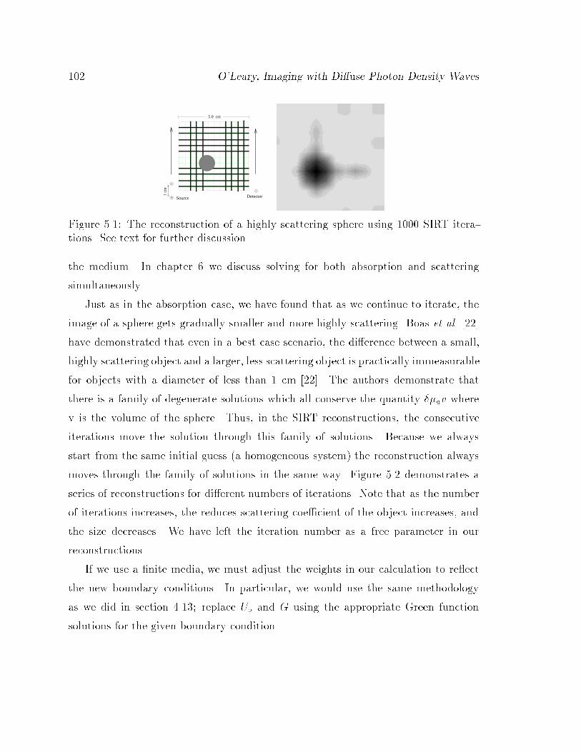
102 O'Leary, Imaging with Di�use Photon Density Waves
5.0 cm
1 cm
-
+ DetectorSource
Figure 5.1: The reconstruction of a highly scattering sphere using 1000 SIRT itera-
tions. See text for further discussion.
the medium. In chapter 6 we discuss solving for both absorption and scattering
simultaneously.
Just as in the absorption case, we have found that as we continue to iterate, the
image of a sphere gets gradually smaller and more highly scattering. Boas et al. [22]
have demonstrated that even in a best case scenario, the di�erence between a small,
highly scattering object and a larger, less scattering object is practically immeasurable
for objects with a diameter of less than 1 cm [22]. The authors demonstrate that
there is a family of degenerate solutions which all conserve the quantity ��av where
v is the volume of the sphere. Thus, in the SIRT reconstructions, the consecutive
iterations move the solution through this family of solutions. Because we always
start from the same initial guess (a homogeneous system) the reconstruction always
moves through the family of solutions in the same way. Figure 5.2 demonstrates a
series of reconstructions for di�erent numbers of iterations. Note that as the number
of iterations increases, the reduces scattering coe�cient of the object increases, and
the size decreases. We have left the iteration number as a free parameter in our
reconstructions.
If we use a �nite media, we must adjust the weights in our calculation to re ect
the new boundary conditions. In particular, we would use the same methodology
as we did in section 4.13; replace Uo and G using the appropriate Green function
solutions for the given boundary condition.
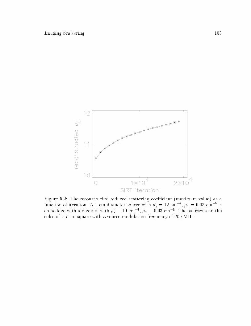
Imaging Scattering 103
Figure 5.2: The reconstructed reduced scattering coe�cient (maximum value) as a
function of iteration. A 1 cm diameter sphere with �0s = 12 cm�1, �a = 0.03 cm�1 is
embedded with a medium with �0s = 10 cm�1, �a = 0.03 cm�1. The sources scan the
sides of a 7 cm square with a source modulation frequency of 200 MHz.

104 O'Leary, Imaging with Di�use Photon Density Waves
Chapter 6
Absorption and Scattering
When we have both variations in both absorption and scattering, the solution to the
heterogeneous di�usion equation is a superposition of our previous solutions. The
Born Solution is
Usc(rd; rs) = �
ZVdr rUo(r; rs) � rG(r� rd)
�D(r)
Do
(6.1)
+
ZVUo(r; rs)G(r� rd)
v��a(r)
Do
; (6.2)
and the Rytov is
�sc(rd; rs) = �1
Uo(rd; rs)
ZVdr rUo(r; rs) � rG(r� rd)
�D(r)
Do
(6.3)
+1
Uo(rd; rs)
ZVUo(r; rs)G(r� rd)
v��a(r)
Do
: (6.4)
This leads us to the following matrices to invert,
Born
0BBBBB@
Usc(rs1; rd1)
...
Usc(rsm; rdm)
1CCCCCA=
0BBBBB@
WBA11
: : : WBA1n WBS
11: : : WBS
1n
.... . .
......
. . ....
WBAm1
: : : WBAmn WBS
m1: : : WBS
mn
1CCCCCA
0BBBBBBBBBBBBBBBBBBBB@
��a(r1)
...
��a(rn)
�D(r1)
...
�D(rn)
1CCCCCCCCCCCCCCCCCCCCA
105
106 O'Leary, Imaging with Di�use Photon Density Waves
WBAij = �Uo(rj; rsi) �G(rdi � rj)vh
3=Do (6.5)
WBSij = rUo(rj; rsi) � rG(rdi � rj)vh
3=Do (6.6)
Rytov
0BBBBB@
�sc(rs1; rd1)
...
�sc(rsm; rdm)
1CCCCCA=
0BBBBB@
WRA11
: : : WRA1n WRS
11: : : WRS
1n
.... . .
......
. . ....
WRAm1
: : : WRAmn WRS
m1: : : WRS
mn
1CCCCCA
0BBBBBBBBBBBBBBBBBBBB@
��a(r1)
...
��a(rn)
�D(r1)
...
�D(rn)
1CCCCCCCCCCCCCCCCCCCCA
WRAij = �Uo(rj; rsi) �G(rdi � rj)vh
3=(Uo(rdi; rsj)Do) (6.7)
WRSij = rUo(rj; rsi) � rG(rdi � rj)vh
3=(Uo(rdi; rsj)Do) (6.8)
We use these matrices, and the save inversion techniques (SIRT, SVD) to create
separate images of absorption and scatttering.
6.1 Simulation Results
For the following simulations the forward data were generated using the exact solution
for one or more spheres embedded in an otherwise homogeneous in�nite medium [10].
Random noise (0.5% amplitude and 0.5o phase) was added to all simulated data.
Unless otherwise stated, the background optical properties of the medium were �a =
0.05 cm�1, �0s = 10.0 cm�1 and the source modulation frequency is 500MHz. The
sources and detectors rotate around a 6.0 cm diameter cylindrical region making a
measurement every 20 degrees. The reconstructed area is broken up into 0.25 cm by
0.25 cm pixels and 2000 SIRT iterations were performed. The two-source subtraction
technique was not used here. For simplicity, the analytic solution for the incident
wave was subtracted as part of the simulation.
Absorption and Scattering 107
We have reconstructed images of scattering and absorption simultaneously using
the Rytov approximation. The results of such a reconstruction are shown in �gure
6.1, where 4 samples are considered.
In the �rst sample, there is only an absorbing inhomogeneity as veri�ed by the
reconstruction. In the second sample there is only a scattering inhomogeneity, how-
ever the reconstruction produced some noise in the absorption map. We see that
an absorbing and a scattering object can be individually imaged. The third sample
demonstrates that we can simultaneously image two objects, one absorbing object
and one scattering object. Note in the fourth panel a single sphere with di�erent
absorption and scattering factor is imaged. We have displaced the scattering and
absorption features in the �gure to emphasize this point.
An important practical advantage of the Rytov approximation is its natural sep-
aration of the amplitude and phase. As stated in equation 5.45, the scattered phase
is the logarithm of the ratio of the measured signals; written
�sc = ln[U=Uo] = ln[Aexp(i�)=Ao exp(i�o)] = ln[A=Ao] + i(�� �o): (6:9)
Thus the amplitude decay corresponds to the real part of the integral, and the phase
shift to the imaginary. Figure 6.2 shows that at 500 MHz, the amplitude ratio
(i.e. amplitude with inhomogeneity relative to amplitude without inhomogeneity)
and phase change for various objects with either a pure scattering change or absorp-
tion change. We see that scattering and absorption changes a�ect the amplitude to
the same degree. However, scattering changes a�ect the phase a great deal more than
an absorption change.
This suggests that the scattering (absorption) reconstructions might be done in-
dependently using just the phase (amplitude) of the measured wave. The results of
this procedure are presented in �gure 6.3. This simulation suggests that while the
scattering reconstruction using only phase data is quite successful, the absorption
reconstruction using only amplitude data is quite noisy.
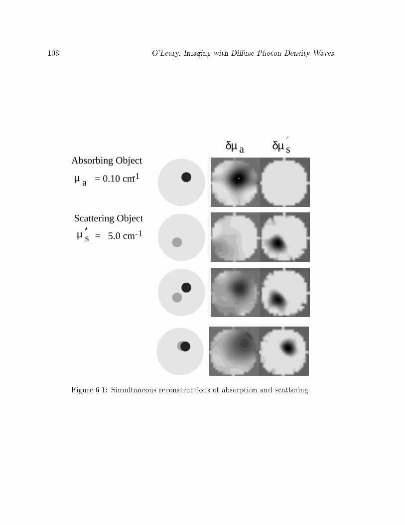
108 O'Leary, Imaging with Di�use Photon Density Waves
aµ
= 5.0 cms -1
= 0.10 cm
µ
-1
µδ a
Scattering Object
Absorbing Object
δµ s
Figure 6.1: Simultaneous reconstructions of absorption and scattering.
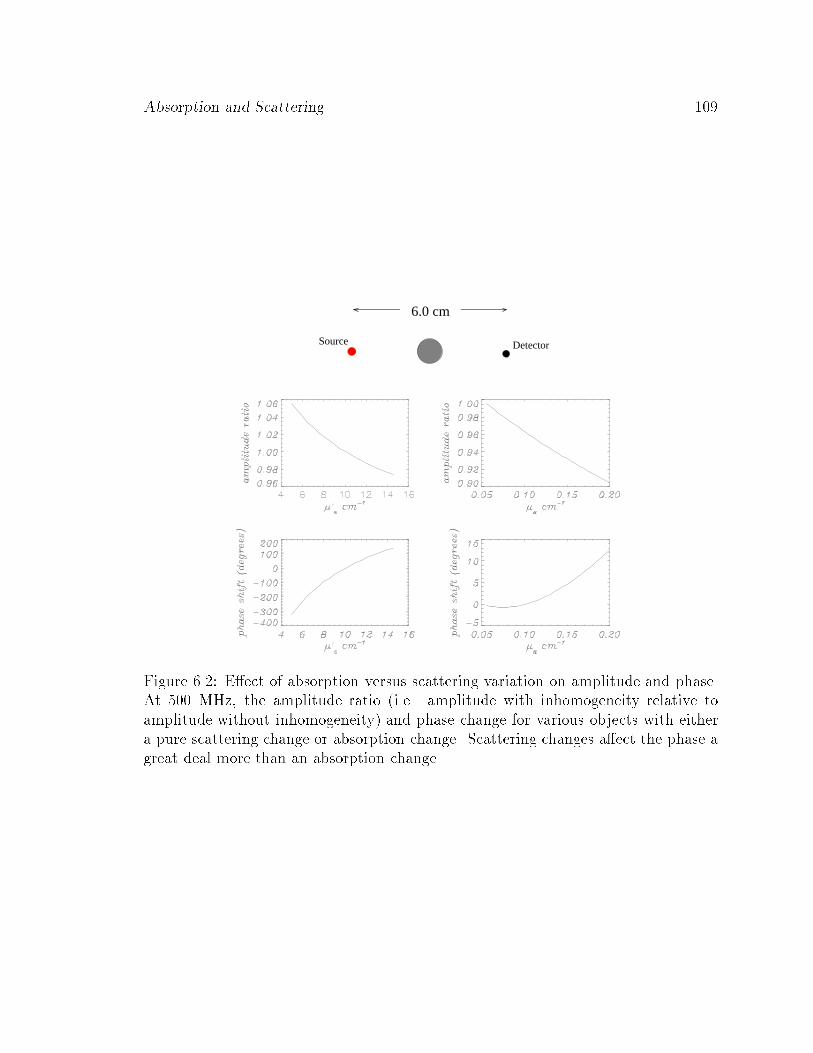
Absorption and Scattering 109
6.0 cm
DetectorSource
Figure 6.2: E�ect of absorption versus scattering variation on amplitude and phase.
At 500 MHz, the amplitude ratio (i.e. amplitude with inhomogeneity relative to
amplitude without inhomogeneity) and phase change for various objects with either
a pure scattering change or absorption change. Scattering changes a�ect the phase a
great deal more than an absorption change.
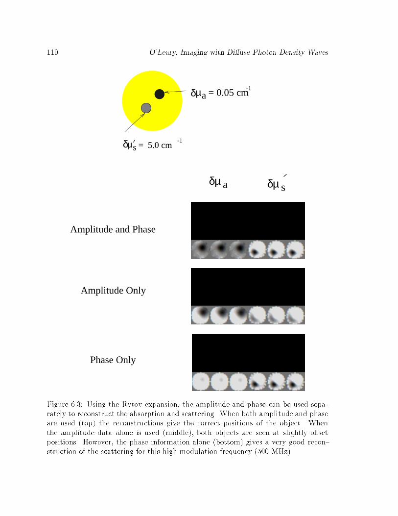
110 O'Leary, Imaging with Di�use Photon Density Waves
a = 0.05 cm-1µ
-1µs = 5.0 cm
a µδ s
Amplitude and Phase
δ
δ
δ
µ
Amplitude Only
Phase Only
Figure 6.3: Using the Rytov expansion, the amplitude and phase can be used sepa-
rately to reconstruct the absorption and scattering. When both amplitude and phase
are used (top) the reconstructions give the correct positions of the object. When
the amplitude data alone is used (middle), both objects are seen at slightly o�set
positions. However, the phase information alone (bottom) gives a very good recon-
struction of the scattering for this high modulation frequency (500 MHz).
Chapter 7
Imaging Fluorescence
We have discussed schemes designed to detect and image heterogeneities in biolog-
ical tissues with di�using near-infrared (NIR) light. These studies have centered
on the detection of variations in the absorption and scattering coe�cients in tissue
and tissue phantoms. Recently however, uorescent contrast agents have also been
considered as a means to enhance the speci�city and sensitivity in tumor detection
[7, 11, 67, 68, 69, 70, 71, 33]. Fluorescent lifetime-based quantitation of di�erent
biological parameters such as tissue oxygenation pO2 [72], pH value [73] and intracel-
lular calcium concentration [Ca2+] [74] have been proposed by several investigators.
Localized uorophore concentration
may signal an increased number of small blood vessels associated with rapid tumor
growth [75]. The altered concentration of a uorophore quencher (such as oxygen)
which a�ects the uorophore lifetime may signal the high oxygen uptake in a rapidly
growing tumor [76]. Thus functional imaging of the variations of uorophore concen-
tration and lifetime may provide useful clinical information.
Much e�ort has been devoted to formulate the forward problem of uorescent light
in turbid media. An integral form in the time domain has been given by Huthcin-
son et al. for the migration of uorescent light in turbid media; these investigators
have also numerically solved this integral equation in speci�c two-dimensional homo-
geneous and heterogeneous systems [21, 77]. A mathematical model for frequency
domain uorescent light propagation in semi-in�nite homogeneous turbid media has
been obtained by Patterson et al. using zero boundary conditions and assuming that
111
112 O'Leary, Imaging with Di�use Photon Density Waves
the reduced scattering coe�cients are the same for the excitation and emission light
[68]. A useful algorithm has been developed by Wu et al. to deconvolve uorescent
emission spectra from tissue re ectance measurements [78]. Finally, in our lab, Li et
al. [79] have presented analytic solutions for uorescent di�use photon density waves
in homogeneous and heterogeneous turbid media with planar boundaries. The fre-
quency domain analysis can easily be applied to time domain experiments by Fourier
transformation of the time domain data.
In this chapter we will �rst discuss the equations which describe the passage of
photons through a uorescent medium. Next we examine the limited case in which
we wish to detect and localize the center of a uorescent object. Finally, we turn
our attention to the more complicated problem of tomographic image reconstruction
techniques for uorescence lifetime imaging in turbid media [12].
Identifying and localizing a tumor becomes a simple procedure if we can turn
a tumor into a source using exogenous uorescent contrast agents. Although there
are currently no FDA approved uorescent contrast agents which speci�cally bind to
tumor sites, the rapid growth of a tumor results in increased vascularity in the region
and an abundance of leaky blood vessels. Certain molecules, such as the popular
MRI contrast agent gadolinium chelate, are known to leak from blood vessels and
accumulate in the intravascular space. Other contrast agents of the same molecular
size, such as indo cyanine green (ICG) are expected to similarly accumulate at the
tumor site. Preliminary studies show a three fold increase in the amount of ICG in
rat tumor compared to normal tissue [70]. ICG is an excellent choice for NIR imaging
since it has an absorption peak at 780 nm, uoresces at 830 nm, and is currently used
in humans to test hepatic and cardiac function [80].
7.1 Fluorescent Di�use Photon Density Wave Theory
In this section we will develop the theory of di�usive waves propagating through
uorescent media. In this analysis, the uorescent radiation is assumed to be well
separated in energy from that of incident photons so that we safely ignore the possi-
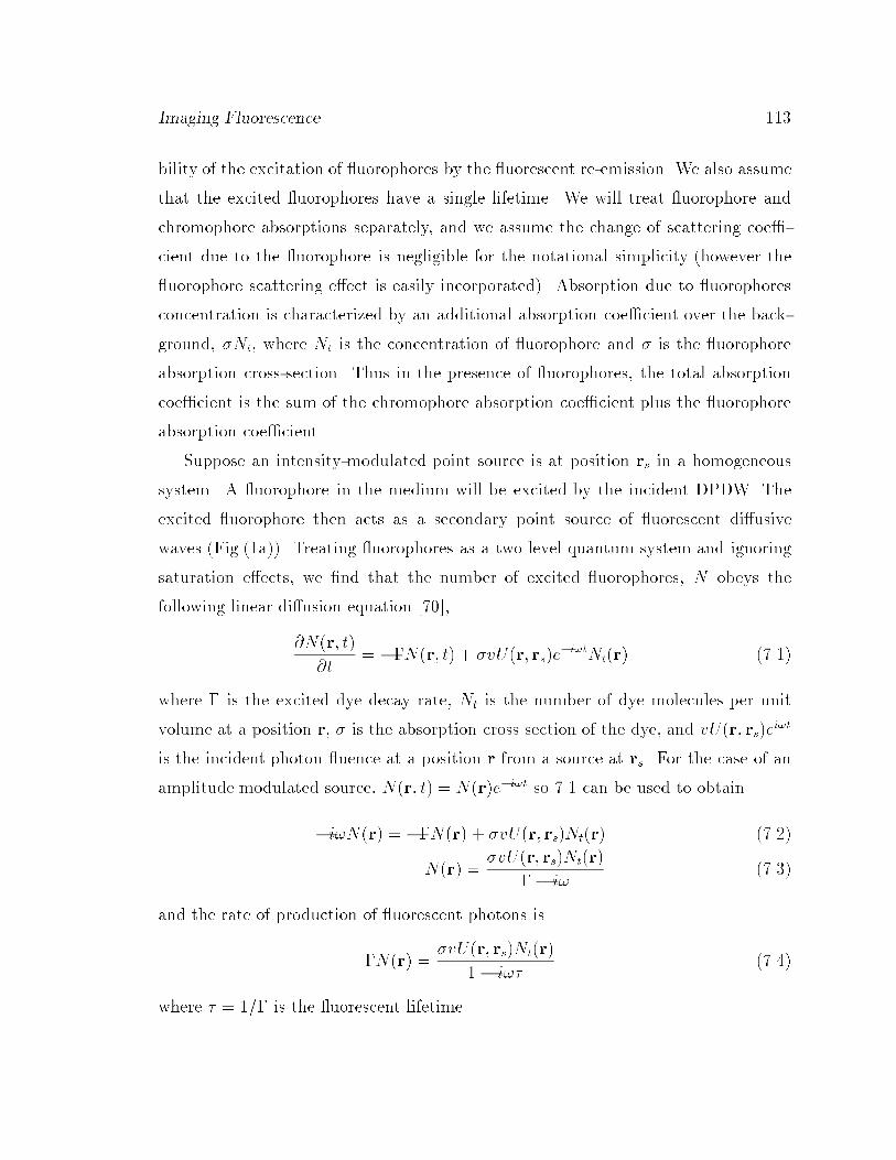
Imaging Fluorescence 113
bility of the excitation of uorophores by the uorescent re-emission. We also assume
that the excited uorophores have a single lifetime. We will treat uorophore and
chromophore absorptions separately, and we assume the change of scattering coe�-
cient due to the uorophore is negligible for the notational simplicity (however the
uorophore scattering e�ect is easily incorporated). Absorption due to uorophores
concentration is characterized by an additional absorption coe�cient over the back-
ground, �Nt, where Nt is the concentration of uorophore and � is the uorophore
absorption cross-section. Thus in the presence of uorophores, the total absorption
coe�cient is the sum of the chromophore absorption coe�cient plus the uorophore
absorption coe�cient.
Suppose an intensity-modulated point source is at position rs in a homogeneous
system. A uorophore in the medium will be excited by the incident DPDW. The
excited uorophore then acts as a secondary point source of uorescent di�usive
waves (Fig.(1a)). Treating uorophores as a two level quantum system and ignoring
saturation e�ects, we �nd that the number of excited uorophores, N obeys the
following linear di�usion equation [70],
@N(r; t)
@t= ��N(r; t) + �vU(r; rs)e
�i!tNt(r) (7.1)
where � is the excited dye decay rate, Nt is the number of dye molecules per unit
volume at a position r, � is the absorption cross section of the dye, and vU(r; rs)ei!t
is the incident photon uence at a position r from a source at rs. For the case of an
amplitude modulated source, N(r; t) = N(r)e�i!t so 7.1 can be used to obtain
�i!N(r) = ��N(r) + �vU(r; rs)Nt(r) (7.2)
N(r) =�vU(r; rs)Nt(r)
�� i!(7.3)
and the rate of production of uorescent photons is
�N(r) =�vU(r; rs)Nt(r)
1� i!�(7.4)
where � = 1=� is the uorescent lifetime.
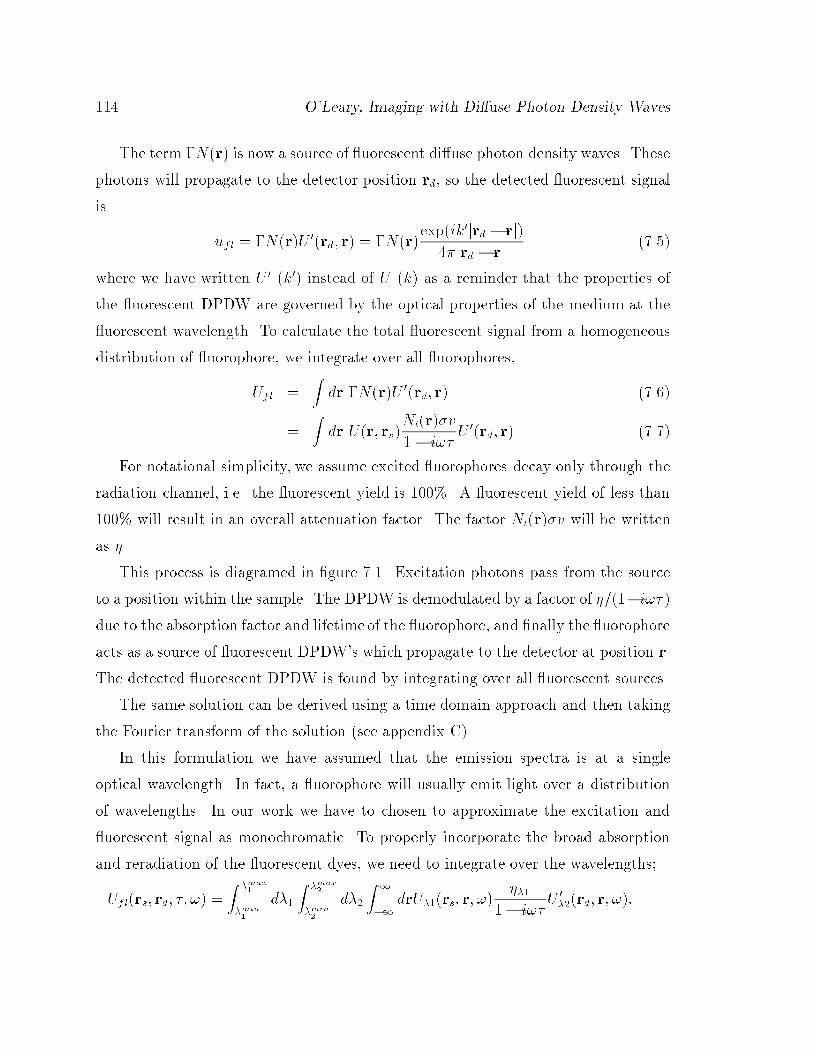
114 O'Leary, Imaging with Di�use Photon Density Waves
The term �N(r) is now a source of uorescent di�use photon density waves. These
photons will propagate to the detector position rd, so the detected uorescent signal
is
ufl = �N(r)U 0(rd; r) = �N(r)exp(ik0jrd � rj)
4�jrd � rj(7.5)
where we have written U 0 (k0) instead of U (k) as a reminder that the properties of
the uorescent DPDW are governed by the optical properties of the medium at the
uorescent wavelength. To calculate the total uorescent signal from a homogeneous
distribution of uorophore, we integrate over all uorophores,
Ufl =Zdr �N(r)U 0(rd; r) (7.6)
=Zdr U(r; rs)
Nt(r)�v
1� i!�U 0(rd; r) (7.7)
For notational simplicity, we assume excited uorophores decay only through the
radiation channel, i.e. the uorescent yield is 100%. A uorescent yield of less than
100% will result in an overall attenuation factor. The factor Nt(r)�v will be written
as �.
This process is diagramed in �gure 7.1. Excitation photons pass from the source
to a position within the sample. The DPDW is demodulated by a factor of �=(1�i!� )
due to the absorption factor and lifetime of the uorophore, and �nally the uorophore
acts as a source of uorescent DPDW's which propagate to the detector at position r.
The detected uorescent DPDW is found by integrating over all uorescent sources.
The same solution can be derived using a time domain approach and then taking
the Fourier transform of the solution (see appendix C).
In this formulation we have assumed that the emission spectra is at a single
optical wavelength. In fact, a uorophore will usually emit light over a distribution
of wavelengths. In our work we have to chosen to approximate the excitation and
uorescent signal as monochromatic. To properly incorporate the broad absorption
and reradiation of the uorescent dyes, we need to integrate over the wavelengths;
Ufl(rs; rd; �; !) =Z �max
1
�min1
d�1
Z �max2
�min2
d�2
Z1
�1
drU�1(rs; r; !)��1
1� i!�U 0
�2(rd; r; !):
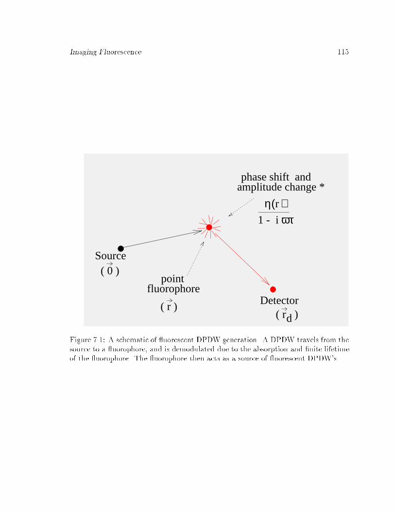
Imaging Fluorescence 115
fluorophorepoint
1 - i
η( )ωτ
r
Source
Detector
phase shift andamplitude change *
d( r )
( 0 )
( r )
Figure 7.1: A schematic of uorescent DPDW generation. A DPDW travels from thesource to a uorophore, and is demodulated due to the absorption and �nite lifetimeof the uorophore. The uorophore then acts as a source of uorescent DPDW's.
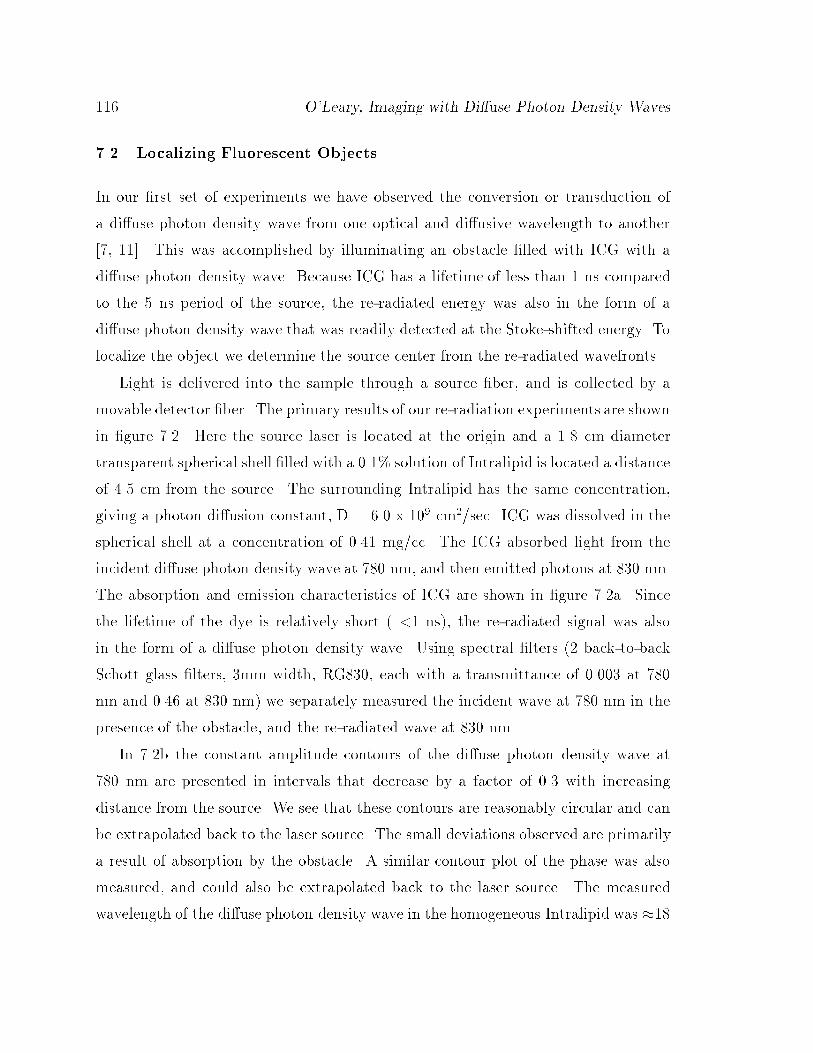
116 O'Leary, Imaging with Di�use Photon Density Waves
7.2 Localizing Fluorescent Objects
In our �rst set of experiments we have observed the conversion or transduction of
a di�use photon density wave from one optical and di�usive wavelength to another
[7, 11]. This was accomplished by illuminating an obstacle �lled with ICG with a
di�use photon density wave. Because ICG has a lifetime of less than 1 ns compared
to the 5 ns period of the source, the re-radiated energy was also in the form of a
di�use photon density wave that was readily detected at the Stoke-shifted energy. To
localize the object we determine the source center from the re-radiated wavefronts.
Light is delivered into the sample through a source �ber, and is collected by a
movable detector �ber. The primary results of our re-radiation experiments are shown
in �gure 7.2. Here the source laser is located at the origin and a 1.8 cm diameter
transparent spherical shell �lled with a 0.1% solution of Intralipid is located a distance
of 4.5 cm from the source. The surrounding Intralipid has the same concentration,
giving a photon di�usion constant, D = 6.0 x 109 cm2/sec. ICG was dissolved in the
spherical shell at a concentration of 0.41 mg/cc. The ICG absorbed light from the
incident di�use photon density wave at 780 nm, and then emitted photons at 830 nm.
The absorption and emission characteristics of ICG are shown in �gure 7.2a. Since
the lifetime of the dye is relatively short ( <1 ns), the re-radiated signal was also
in the form of a di�use photon density wave. Using spectral �lters (2 back-to-back
Schott glass �lters, 3mm width, RG830, each with a transmittance of 0.003 at 780
nm and 0.46 at 830 nm) we separately measured the incident wave at 780 nm in the
presence of the obstacle, and the re-radiated wave at 830 nm.
In 7.2b the constant amplitude contours of the di�use photon density wave at
780 nm are presented in intervals that decrease by a factor of 0.3 with increasing
distance from the source. We see that these contours are reasonably circular and can
be extrapolated back to the laser source. The small deviations observed are primarily
a result of absorption by the obstacle. A similar contour plot of the phase was also
measured, and could also be extrapolated back to the laser source. The measured
wavelength of the di�use photon density wave in the homogeneous Intralipid was �18
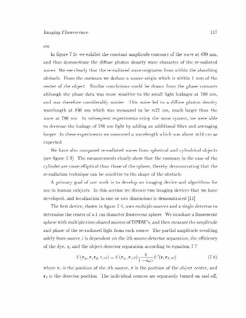
Imaging Fluorescence 117
cm.
In �gure 7.2c we exhibit the constant amplitude contours of the wave at 830 nm,
and thus demonstrate the di�use photon density wave character of the re-radiated
waves. We see clearly that the re-radiated wave originates from within the absorbing
obstacle. From the contours we deduce a source origin which is within 1 mm of the
center of the object. Similar conclusions could be drawn from the phase contours
although the phase data was more sensitive to the small light leakages at 780 nm,
and was therefore considerably noisier. This noise led to a di�use photon density
wavelength at 830 nm which was measured to be �27 cm, much larger than the
wave at 780 nm. In subsequent experiments using the same system, we were able
to decrease the leakage of 780 nm light by adding an additional �lter and averaging
longer. In these experiments we measured a wavelength which was about �18 cm as
expected.
We have also compared re-radiated waves from spherical and cylindrical objects
(see �gure 7.3). The measurements clearly show that the contours in the case of the
cylinder are more elliptical than those of the sphere, thereby demonstrating that the
re-radiation technique can be sensitive to the shape of the obstacle.
A primary goal of our work is to develop an imaging device and algorithms for
use in human subjects. In this section we discuss two imaging devices that we have
developed, and localization in one or two dimensions is demonstrated [11].
The �rst device, shown in �gure 7.4, uses multiple sources and a single detector to
determine the center of a 1 cm diameter uorescent sphere. We irradiate a uorescent
sphere with multiple time-shared sources of DPDW's, and then measure the amplitude
and phase of the re-radiated light from each source. The partial amplitude resulting
solely from source i is dependent on the ith source-detector separation, the e�ciency
of the dye, �, and the object-detector separation according to equation 7.7
U(rsi; r; rd; �; !) = U(rsi; r; !)�
1� i!�U 0(r; rd; !) (7.8)
where ri is the position of the ith source, r is the position of the object center, and
rd is the detector position. The individual sources are separately turned on and o�,

118 O'Leary, Imaging with Di�use Photon Density Waves
800Wavelength (nm)
Em
issi
on In
tens
ity (
arb.
uni
ts)
850 900750
Absorbance
2
4
0
-2
-40 -2 -4 -6 -8
cm
cm
(a) (b)
20
40
0
0.5
1.0
2
4
0
-2
-40 -2 -4 -6 -8
cm
cm
(c)
Figure 7.2: (a) Indocyanine green absorption (solid line) and emission (dashed line)
spectra. (b) Constant amplitude contours of the incident di�use photon density wave.(c) Constant amplitude contours at the uorescent wavelength (solid lines) clearlyexhibiting the re-radiated nature of the wave. The dashed lines are the incidentamplitude contours, and the center of the radiator is located by �nding the intersectionof the lines normal to the re-radiated contours.
6
2
0
4
0 2 4-2-40 2 4-2-4
6
2
0
4
ln(Amplitude) Phase
Figure 7.3: left: Constant amplitude contours of the uorescent DPDW re-radiatedfrom a cylindrical uorescent object. The source is at the origin. The contours are
drawn every 0.3 dBm. right: The contours of constant phase, drawn every 10� . The
dashed lines are interpolated data.
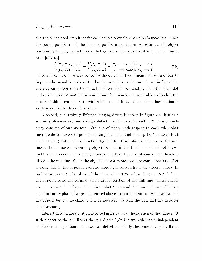
Imaging Fluorescence 119
and the re-radiated amplitude for each source-obstacle separation is measured. Since
the source positions and the detector positions are known, we estimate the object
position by �nding the value or r that gives the best agreement with the measured
ratio jUij=jUjj.
U(rsi; r; rd; �; !)
U(rsj; r; rd; �; !)=
U(rsi; r; !)
U(rsj; r; !)=jrsj � rj
jrsi � rj
exp(ikjrsi � rj)
exp(ikjrsj � rj): (7.9)
Three sources are necessary to locate the object in two dimensions, we use four to
improve the signal to noise of the localization. The results are shown in �gure 7.5;
the grey circle represents the actual position of the re-radiator, while the black dot
is the computer estimated position. Using four sources we were able to localize the
center of this 1 cm sphere to within 0.4 cm. This two dimensional localization is
easily extended to three dimensions.
A second, qualitatively di�erent imaging device is shown in �gure 7.6. It uses a
scanning phased-array and a single detector as discussed in section 2. The phased-
array consists of two sources, 180� out of phase with respect to each other that
interfere destructively to produce an amplitude null and a sharp 180� phase shift at
the null line (broken line in insets of �gure 7.6). If we place a detector on the null
line, and then move an absorbing object from one side of the detector to the other, we
�nd that the object preferentially absorbs light from the nearest source, and therefore
distorts the null line. When the object is also a re-radiator, the complimentary e�ect
is seen, that is, the object re-radiates more light derived from the closest source. In
both measurements the phase of the detected DPDW will undergo a 180� shift as
the object crosses the original, undisturbed position of the null line. These e�ects
are demonstrated in �gure 7.6a. Note that the re-radiated wave phase exhibits a
complimentary phase change as discussed above. In our experiments we have scanned
the object, but in the clinic it will be necessary to scan the pair and the detector
simultaneously.
Interestingly, in the situation depicted in �gure 7.6a, the location of the phase shift
with respect to the null line of the re-radiated light is always the same, independent
of the detector position. Thus we can detect essentially the same change by �xing
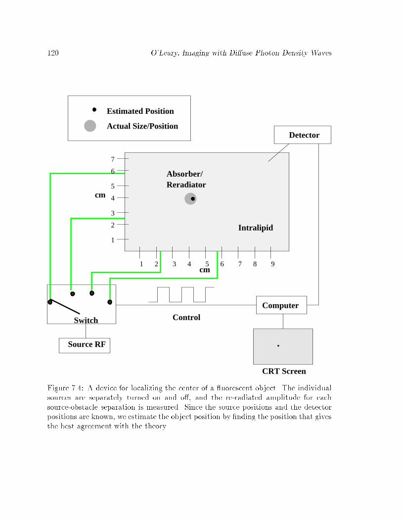
120 O'Leary, Imaging with Di�use Photon Density Waves
Estimated Position
Actual Size/Position
CRT Screen
ComputerControl
Source RF
Switch
Intralipid
cm
cm
Detector
7
6
5
4
3
2
1
Absorber/Reradiator
98654321 7
Figure 7.4: A device for localizing the center of a uorescent object. The individualsources are separately turned on and o�, and the re-radiated amplitude for each
source-obstacle separation is measured. Since the source positions and the detectorpositions are known, we estimate the object position by �nding the position that gives
the best agreement with the theory.
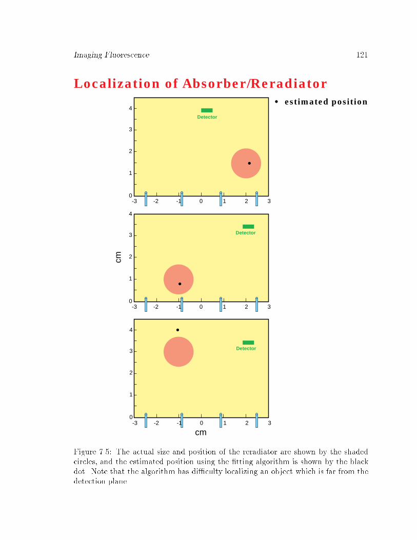
Imaging Fluorescence 121
4
3
2
1
0-3 -2 -1 0 1 2 3
4
3
2
1
0
4
3
2
1
0
Detector
Detector
-3 -2 -1 0 1 2 3
-3 -2 -1 0 1 2 3
cm
cm
Detector
Localization of Absorber/Reradiatorestimated position
Figure 7.5: The actual size and position of the reradiator are shown by the shaded
circles, and the estimated position using the �tting algorithm is shown by the blackdot. Note that the algorithm has di�culty localizing an object which is far from the
detection plane.
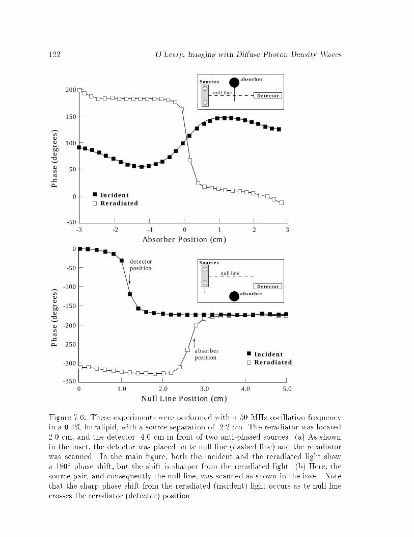
122 O'Leary, Imaging with Di�use Photon Density Waves
200
150
100
50
0
-50-3 -2 -1 0 1 2 3
Absorber Position (cm)
Ph
ase
(deg
rees
)
IncidentReradiated
-50
0
-100
-150
-200
-250
-300
-3500 1.0 2.0 3.0 4.0 5.0
Null Line Position (cm)
Ph
ase
(deg
rees
)
IncidentReradiated
Detector
Sources absorber
absorberposition
detectorposition
Detector
Sources
absorber
+
–
+
–
null line
null line
Figure 7.6: These experiments were performed with a 50 MHz oscillation frequencyin a 0.4% Intralipid, with a source separation of 2.2 cm. The reradiator was located
2.0 cm, and the detector 4.0 cm in front of two anti-phased sources. (a) As shown
in the inset, the detector was placed on te null line (dashed line) and the reradiatorwas scanned. In the main �gure, both the incident and the reradiated light show
a 180� phase shift, but the shift is sharper from the reradiated light. (b) Here, thesource pair, and consequently the null line, was scanned as shown in the inset. Note
that the sharp phase shift from the reradiated (incident) light occurs as te null line
crosses the reradiator (detector) position
Imaging Fluorescence 123
the object and the detector, and scanning only the source pair. This con�guration is
more clinically realizable than the absorption case which requires scanning both the
source pair and the detector. Figure 7.6b demonstrates this e�ect for the re-radiated
light. In the left panel, we detect a sharp phase shift for the location of the re-radiator
as we scan the null line. The phase shift of the incident light occurs near the position
of the detector. If we know the position of the null line as a function of time, we
achieve a one dimensional localization of the re-radiator. By performing three scans
down three perpendicular axis, we can achieve three dimensional localization.
7.3 Tomographic Imaging of Fluorescent Objects
So far, we have discussed using di�use uorescence in deep tissues as a means of
tumor detection and localization by imaging the center of uorescing objects. In this
section we demonstrate a more general method whereby one can simultaneously derive
a spatial map of the concentration and lifetime of a uorophore, using variations in
the amplitude and phase of uorescent di�use photon density waves.
For a weakly absorbing spatial distribution of uorophores, the uorescent photon
density wave is determined by integrating over the contributions from all uorophores
as in equation 7.7.
Ufl(rs; rd; �; !) =Zd3r U(rs; r; !)
�(r)
1� i!� (r)U 0(r; rd; !): (7.10)
Note that we have allowed � and � to vary with position.
Hereafter we refer to Ufl as the uorescent di�use photon density wave. In a
heterogeneous medium this model is an approximation in the sense that the homo-
geneous solution neglects the e�ects of heterogeneities on photon propagation from
source to uorophore and from uorophore to detector. The model also assumes that
there are no saturation or photon quenching e�ects.
The uorescence model in equation 7.10 is of the same form as the �rst order Born
approximation solution for a scattering medium with inhomogeneous absorption, i.e.
124 O'Leary, Imaging with Di�use Photon Density Waves
equation 4.13,
Usc(rs; rd; !) = �ZU(rs; r; !)O(r)U
0(r; rd; !) d3r: (7.11)
Thus we are able to generate images for �(r) and � (r) using standard imaging al-
gorithms. The reconstruction di�ers from the pure absorption case in that the re-
constructed quantity is now complex, and is a function of the modulation frequency.
Again, the reconstruction algorithm involves digitizing the integral in equation 7.10
(�(r); � (r); r ) �j; �j; rj), and for a series of measurements made at source-detector
positions rsi, rdi, we generate the following matrix equation:
Ufl(rsi; rdi; !) =NvoxelsXj=1
U(rj ; rsi; !)�j
1� i!�jU 0(rdi; rj; !)h
3: (7.12)
This complex matrix is can be written as a real matrix;
0BBBBBBBBBBBBBBBBBBBB@
<[U[1]
fl ]
...
<[U[m]
fl ]
=[U[1]
fl ]
...
=[U[m]
fl ]
1CCCCCCCCCCCCCCCCCCCCA
=
0BBBBBBBBBBBBBBBBBBBB@
<[W fl11] : : : <[W fl
1n] �=[W fl11] : : : =[W fl
1n]
.... . .
......
. . ....
<[W flm1] : : : <[W fl
mn] �=[W flm1] : : : �=[W fl
mn]
=[W fl11] : : : =[W fl
1n] <[W fl11] : : : <[W fl
1n]
.... . .
......
. . ....
=[W flm1] : : : =[W fl
mn] <[W flm1] : : : <[W fl
mn]
1CCCCCCCCCCCCCCCCCCCCA
0BBBBBBBBBBBBBBBBBBBB@
�(r1)
...
�(rn)
�(r1)
...
�(rn)
1CCCCCCCCCCCCCCCCCCCCA
W flij = U(rj ; rsi; !)U
0(rdi; rj; !)h3 (7.13)
�(rj) = <[�j=(1 � i!�j)] (7.14)
�(rj) = =[�j=(1 � i!�j)] (7.15)
This matrix equation can be inverted or solved using many techniques. We have
used an algebraic reconstruction method (SIRT) to solve for the real (�) and imagi-
nary (�) parts of the unknown, �j=(1� i!�j) [48]. The ratio of the imaginary to the
Imaging Fluorescence 125
real parts of the solution yields � , and then � may be calculated.
�j =�
�!(7.16)
�j = � + !�� (7.17)
Computer generated data are obtained from exact solutions to the uorescence
di�usion equation for the case of a uorescent sphere (1.0 cm diameter) in a uniform
background [79]. Using forward amplitude and phase data from this solution (with
added 1% amplitude and 0.1o phase noise), we have reconstructed images of � and � .
The measurement geometry used is described in �gure 7.9a. The scanning geometry
consists of a source and detector scanning every 0.2 cm around the four sides of a 7.0
cm x 7.0 cm square in an in�nite medium. The reconstruction area is a slab of area
5.0 cm x 5.0 cm and height 1.0 cm. The optical properties of the media are: �0s = 10
cm�1 everywhere, �a (chromophore) = 0.03 cm�1 everywhere for both the excitation
and the emission wavelength, and �a ( uorophore - inside the sphere) = 0.02 cm�1
at the excitation wavelength, and 0.01 cm�1 at the emission wavelength. The source
modulation frequency is 50 MHz. In the �rst set of reconstructions all uorophores
are located in the object and there is no background uorescence.
In �gure 7.9b we demonstrate a reconstruction proportional to the uorophore
concentration. The lifetime inside the 1.0 cm diameter sphere is 0.6 ns. The grey
scale ranges from 0 cm�1 (grey) to 0.007 cm�1 (black). 2500 SIRT iterations were
performed with a constraint on both concentration (0:0 � � � 0:1 cm�1) and lifetime
(0 � � � 10 ns).
Note that the reconstructed value of � is much less than the correct value. This
is due to the fact that we have only performed 2500 SIRT iterations to produce this
image. This relatively small number of SIRT iterations results is an image of a larger
object with a lower concentration of uorophores. This is exactly analogous to the
absorption case where we discovered that as we increase the number of iterations, the
reconstructed object becomes smaller and more absorbing. In the course of imple-
menting these reconstructions we found that some isolated voxels had unphysically
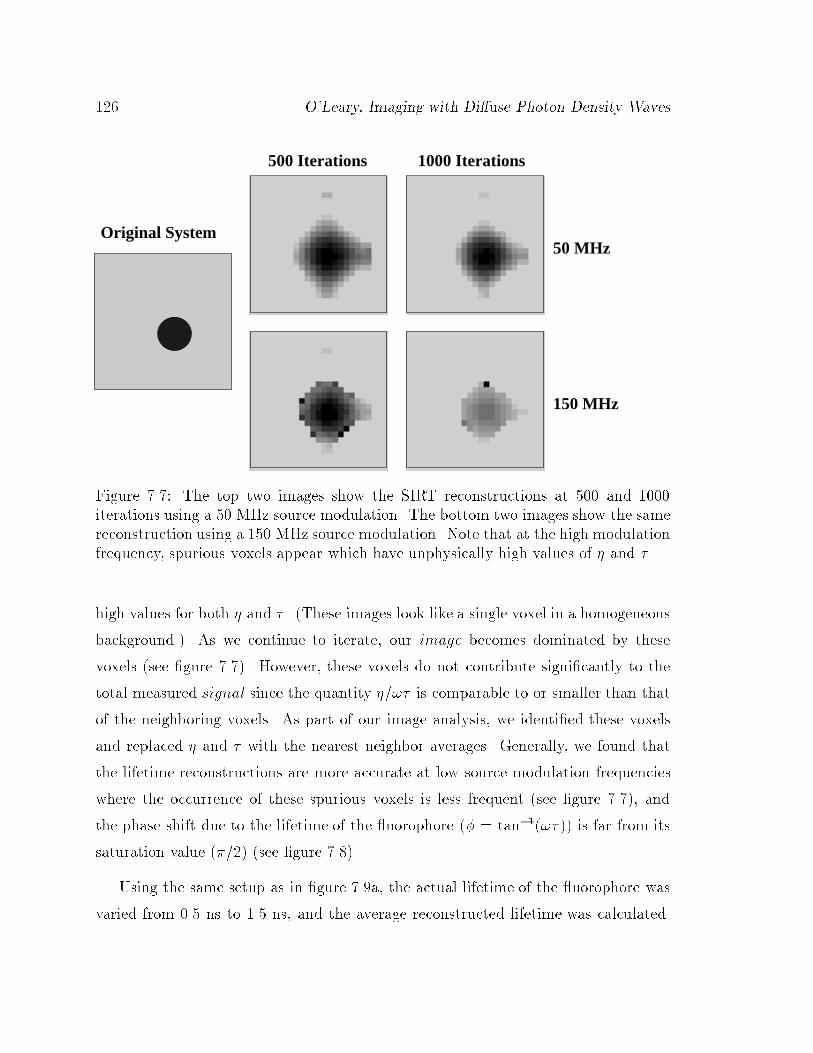
126 O'Leary, Imaging with Di�use Photon Density Waves
Original System
1000 Iterations500 Iterations
50 MHz
150 MHz
Figure 7.7: The top two images show the SIRT reconstructions at 500 and 1000iterations using a 50 MHz source modulation. The bottom two images show the samereconstruction using a 150 MHz source modulation. Note that at the high modulationfrequency, spurious voxels appear which have unphysically high values of � and � .
high values for both � and � . (These images look like a single voxel in a homogeneous
background.) As we continue to iterate, our image becomes dominated by these
voxels (see �gure 7.7). However, these voxels do not contribute signi�cantly to the
total measured signal since the quantity �/!� is comparable to or smaller than that
of the neighboring voxels. As part of our image analysis, we identi�ed these voxels
and replaced � and � with the nearest neighbor averages. Generally, we found that
the lifetime reconstructions are more accurate at low source modulation frequencies
where the occurrence of these spurious voxels is less frequent (see �gure 7.7), and
the phase shift due to the lifetime of the uorophore (� = tan�1(!� )) is far from its
saturation value (�=2) (see �gure 7.8).
Using the same setup as in �gure 7.9a, the actual lifetime of the uorophore was
varied from 0.5 ns to 1.5 ns, and the average reconstructed lifetime was calculated.
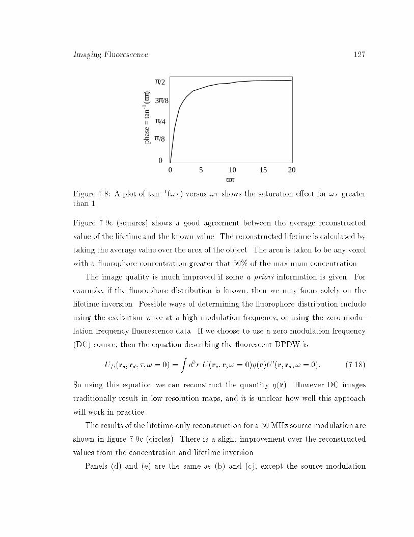
Imaging Fluorescence 127
phas
e =
tan
(
)-1
ωτ
5 10 15 200ωτ
0
/2
/4
/8
3 /8
π
π
π
π
Figure 7.8: A plot of tan�1(!� ) versus !� shows the saturation e�ect for !� greaterthan 1.
Figure 7.9c (squares) shows a good agreement between the average reconstructed
value of the lifetime and the known value. The reconstructed lifetime is calculated by
taking the average value over the area of the object. The area is taken to be any voxel
with a uorophore concentration greater that 50% of the maximum concentration.
The image quality is much improved if some a priori information is given. For
example, if the uorophore distribution is known, then we may focus solely on the
lifetime inversion. Possible ways of determining the uorophore distribution include
using the excitation wave at a high modulation frequency, or using the zero modu-
lation frequency uorescence data. If we choose to use a zero modulation frequency
(DC) source, then the equation describing the uorescent DPDW is
Ufl(rs; rd; �; ! = 0) =Zd3r U(rs; r; ! = 0)�(r)U 0(r; rd; ! = 0): (7.18)
So using this equation we can reconstruct the quantity �(r). However DC images
traditionally result in low resolution maps, and it is unclear how well this approach
will work in practice.
The results of the lifetime-only reconstruction for a 50 MHz source modulation are
shown in �gure 7.9c (circles). There is a slight improvement over the reconstructed
values from the concentration and lifetime inversion.
Panels (d) and (e) are the same as (b) and (c), except the source modulation
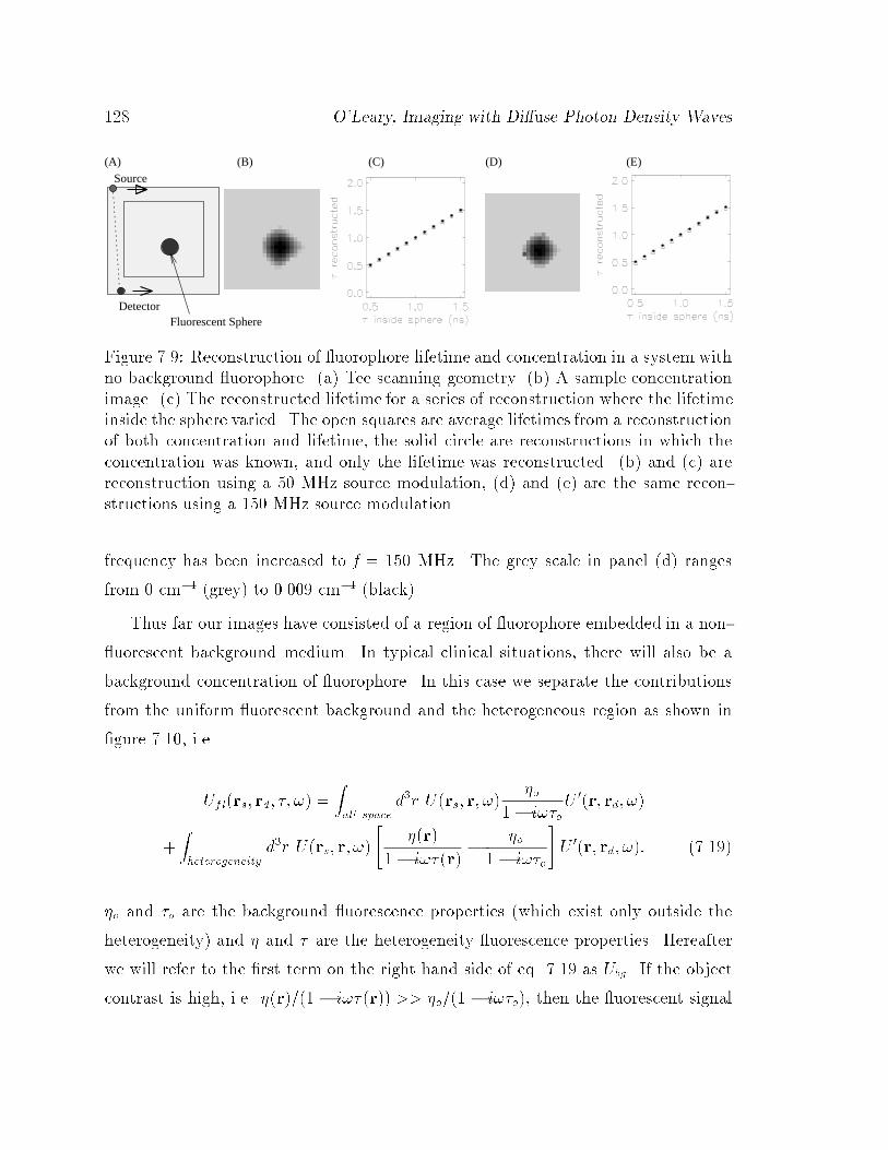
128 O'Leary, Imaging with Di�use Photon Density Waves
(E)(D)(A) (C)(B)
Fluorescent SphereDetector
Source
Figure 7.9: Reconstruction of uorophore lifetime and concentration in a system with
no background uorophore. (a) Tee scanning geometry. (b) A sample concentration
image. (c) The reconstructed lifetime for a series of reconstruction where the lifetimeinside the sphere varied. The open squares are average lifetimes from a reconstructionof both concentration and lifetime, the solid circle are reconstructions in which the
concentration was known, and only the lifetime was reconstructed. (b) and (c) arereconstruction using a 50 MHz source modulation, (d) and (e) are the same recon-structions using a 150 MHz source modulation.
frequency has been increased to f = 150 MHz. The grey scale in panel (d) ranges
from 0 cm�1 (grey) to 0.009 cm�1 (black).
Thus far our images have consisted of a region of uorophore embedded in a non-
uorescent background medium. In typical clinical situations, there will also be a
background concentration of uorophore. In this case we separate the contributions
from the uniform uorescent background and the heterogeneous region as shown in
�gure 7.10, i.e.
Ufl(rs; rd; �; !) =Zall space
d3r U(rs; r; !)�o
1� i!�oU 0(r; rd; !)
+Zheterogeneity
d3r U(rs; r; !)
"�(r)
1 � i!� (r)�
�o
1� i!�o
#U 0(r; rd; !): (7.19)
�o and �o are the background uorescence properties (which exist only outside the
heterogeneity) and � and � are the heterogeneity uorescence properties. Hereafter
we will refer to the �rst term on the right hand side of eq. 7.19 as Ubg. If the object
contrast is high, i.e. �(r)=(1 � i!� (r)) >> �o=(1 � i!�o), then the uorescent signal
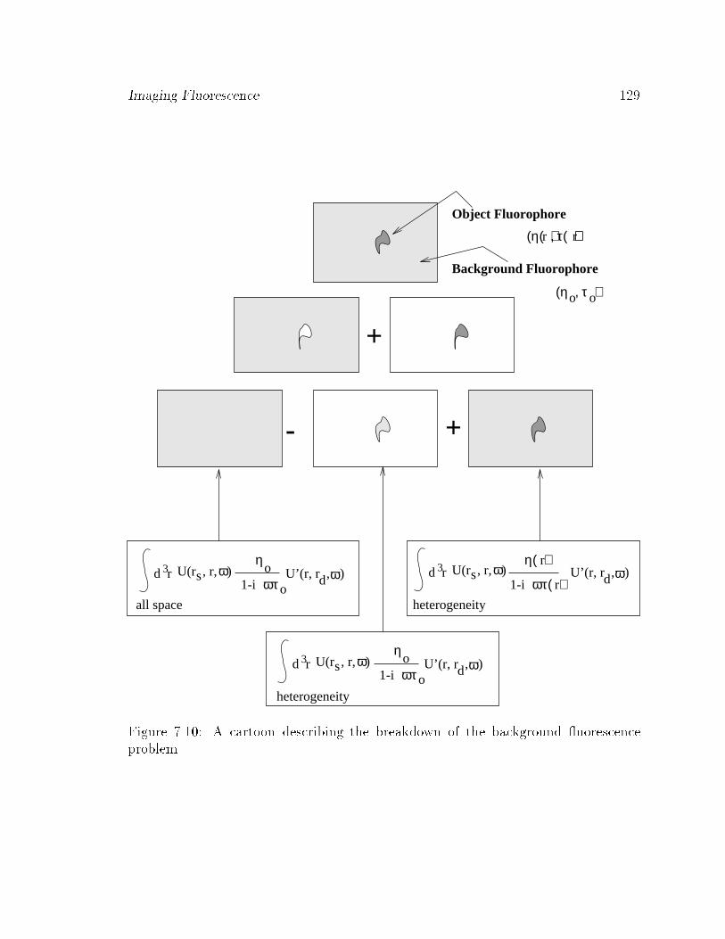
Imaging Fluorescence 129
s ωU(r , r, ) d r3
all space
1-id r3 ωU(r , r, ) s
η( )
ωτ( )rωdU’(r, r , )
heterogeneity
ω
ωτ
r
1-i ωτo
os ωU(r , r, ) d r3
heterogeneity
o o(η , τ )
(η( ), τ( ))rr
η
1-iU’(r, r , ) d
d
o
o
U’(r, r , )
ω
η
Background Fluorophore
Object Fluorophore
+
+-
Figure 7.10: A cartoon describing the breakdown of the background uorescenceproblem.
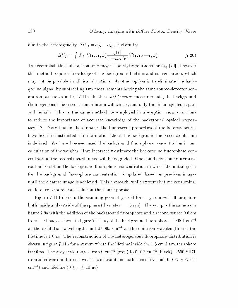
130 O'Leary, Imaging with Di�use Photon Density Waves
due to the heterogeneity, �Ufl = Ufl � Ubg, is given by
�Ufl =Zd3r U(rs; r; !)
�(r)
1� i!� (r)U 0(r; rd � r; !): (7.20)
To accomplish this subtraction, one may use analytic solutions for Ubg [79]. However
this method requires knowledge of the background lifetime and concentration, which
may not be possible in clinical situations. Another option is to eliminate the back-
ground signal by subtracting two measurements having the same source-detector sep-
aration, as shown in �g. 7.11a. In these difference measurements, the background
(homogeneous) uorescent contribution will cancel, and only the inhomogeneous part
will remain. This is the same method we employed in absorption reconstructions
to reduce the importance of accurate knowledge of the background optical proper-
ties [18]. Note that in these images the uorescent properties of the heterogeneities
have been reconstructed; no information about the background uorescence lifetime
is derived. We have however used the background uorophore concentration in our
calculation of the weights. If we incorrectly estimate the background uorophore con-
centration, the reconstructed image will be degraded. One could envision an iterative
routine to obtain the background uorophore concentration in which the initial guess
for the background uorophore concentration is updated based on previous images
until the clearest image is achieved. This approach, while extremely time consuming,
could o�er a more exact solution than our approach.
Figure 7.11d depicts the scanning geometry used for a system with uorophore
both inside and outside of the sphere (diameter = 1.5 cm). The setup is the same as in
�gure 7.9a with the addition of the background uorophore and a second source 0.6 cm
from the �rst, as shown in �gure 7.11. �a of the background uorophore = 0.001 cm�1
at the excitation wavelength, and 0.0005 cm�1 at the emission wavelength and the
lifetime is 1.0 ns. The reconstruction of the heterogeneous uorophore distribution is
shown in �gure 7.11b for a system where the lifetime inside the 1.5 cm diameter sphere
is 0.6 ns. The grey scale ranges from 0 cm�1 (grey) to 0.017 cm�1 (black). 2500 SIRT
iterations were performed with a constraint on both concentration (0:0 � � � 0:1
cm�1) and lifetime (0 � � � 10 ns).
Imaging Fluorescence 131
(C) (D) (E)(A) (B)
BackgroundFluorescent
Fluorescent Sphere
Detector
Sources
Figure 7.11: Reconstruction of uorophore lifetime and concentration in a system
with background uorophore. (a) The scanning geometry. (b) A sample concentra-
tion image. (c) The reconstructed lifetime for a series of reconstruction where thelifetime inside the sphere varied. The open squares are average lifetimes from a re-
construction of both concentration and lifetime, the solid circle are reconstructionsin which the concentration was known, and only the lifetime was reconstructed. (b)and (c) are reconstruction using a 50 MHz source modulation, (d) and (e) are thesame reconstructions using a 150 MHz source modulation.
The average reconstructed lifetime for a series of reconstructions is shown in �gure
7.11a. The squares are derived from a reconstruction of both uorophore concentra-
tion and lifetime. The circles are derived from the lifetime reconstruction only. Panels
(d) and (e) are the same as (b) and (c) except the source modulation frequency has
been increased to f = 150 MHz. The grey scale in panel (D) ranges from 0 cm�1
(grey) to 0.020 cm�1 (black).
We have presented and demonstrated an algorithm by which the heterogeneous
uorophore distribution and lifetime in a turbid medium may be obtained from to-
mographic measurements of near infra-red di�using photon distributions. Although
these reconstructions were carried out from data in the frequency domain, the results
can also be obtained using Fourier transformed time domain data. The solution for
�nite systems may be obtained by applying the appropriate boundary conditions.
Such solutions are readily available for a variety of geometries [59].

132 O'Leary, Imaging with Di�use Photon Density Waves
Chapter 8
Summary
We have demonstrated that di�usive light can be used to image absorption, scattering
and uorescence lifetime and concentration in thick, turbid media. We hope we have
convinced the reader that this work has important medical applications.
There is a great deal of work to be done if DPDW imaging is to become an ac-
cepted medical tool. First and foremost, we need many more studies which accurately
measure the optical changes which accompany changes in the physiological state of
tissues. The intrinsic hetereogeneity of the body makes it di�cult to measure in vivo
the absorption and scattering coe�cients. When tissue samples are studied in vitro,
the blood and oxygen supply is cut o�, thus changing the tissue environment. It is not
clear whether or not in vitro measurements accurately re ect the optical properties
of the sample in vivo.
We believe that DPDW imaging should be used to complement other imaging
modalities. For example, a DPDW probe could be easily attached to an ultrasound,
x-ray, or MRI imaging device as we saw in section 4.12. When the data from these
two probes are used simultaneously. we can derive accurate structural information as
well as quantitative measurements of the optical properties.
DPDW imaging can also be used for low resolution breast tumor screening. There
are several academic and industrial research groups performing clinical evaluations
of optical mammography systems [13, 81, 82]. These studies are particularly exciting
because optical mammography is inexpensive, and has no known adverse side e�ects.
The preliminary results of these studies are encouraging, but a great deal of work still
133
134 O'Leary, Imaging with Di�use Photon Density Waves
needs to be done.
Appendix A
Singular Matrices
A singular matrix is one which maps a vector, (other than the zero vector) to the
zero vector. For example, the matrix
A =
0B@
1 �1
�1 1
1CA (A.1)
maps any vector of the form ~� = (�;�) to the zero vector. This has very important
implications for the inverse solution. Suppose we are trying to invert the following
equation,
A~x = ~b: (A.2)
It is clear that for any solution ~x, ~x+ ~� is also a solution, i.e. if
A~x = ~b (A.3)
and
A~� = ~0 (A.4)
then
A�~b+ ~�
�= A~b+A~� (A.5)
= A~b+~0 = A~b (A.6)
Thus for a singular matrix, there is not a unique solution. Mathematically, a singular
matrix expresses itself as having a zero eigenvalue. In numerical calculations, an
135
136 O'Leary, Imaging with Di�use Photon Density Waves
eigenvalue is rarely exactly equal to zero, but is numerically zero. Numerically zero
means that the value of the number is below the numerical precision of the computer.
Appendix B
Time Resolved Spectroscopy
A schematic of the time resolved spectroscopy system (TRS) is shown in �gure B.1.
The TRS is a single photon counting device built by Hamamatsu Corporation, Japan.
A pulsed laser diode with a full-width half-max of about 50 ps and 5 MHz repetition
rate is coupled to a 200 �mmulti-mode optical �ber. The �ber delivers the light to the
sample, and a 3 mm optical �ber bundle is used to collect the light from the sample.
This second �ber delivers the collected light to a microchannel plate photomultiplier
tube (MCP-PMT)
When a photon strikes the photomultiplier tube, a current is generated, and passed
into a constant fraction discriminator (CFD). The CFD converts a irregularly shaped
pulse into a clean (TTL) step voltage (�gure B.2). This step voltage is passed to
the time amplitude converter (TAC). The TAC is a simple timing device which is
triggered by the same trigger which pulses the laser source. The timing is stopped
when the TAC receives a signal from the CFD. An equivalent circuit is shown in
�gure B.3. A voltage which is proportional to the amount of time between the trigger
and the pulse from the CFD is output from the TAC, to an analog to digital (A/D)
converter. Note that only the �rst photon per pulse will be counted in this system.
For this reason, the source light is attenuated so that no more than one photon per
pulse is detected.
The A/D converter passes a digital number corresponding to the voltage from the
TAC to a multichannel analyzer (MCA). The MCA collects the digital voltage signals
and collects them into corresponding time bins which are stored in the computer. The
137
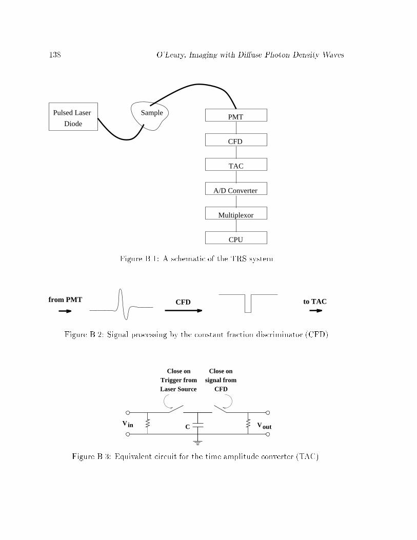
138 O'Leary, Imaging with Di�use Photon Density Waves
Pulsed Laser
Diode
A/D Converter
Multiplexor
CPU
PMT
TAC
CFD
Sample
Figure B.1: A schematic of the TRS system
CFD to TACfrom PMT
Figure B.2: Signal processing by the constant fraction discriminator (CFD)
VoutVin
Close onsignal from
CFD
C
Close onTrigger fromLaser Source
Figure B.3: Equivalent circuit for the time amplitude converter (TAC).
TRS 139
time per bin is calibrated by measuring two signals displaced by a known time delay.
For each pulse, we collect a single photon, and add a count to one bin. This
processes is repeated for millions of pulses (typically we use a 30 second integration
time and a 5 MHz pulse rate) and a histogram of number of photons per time bin is
generated. For examples of TRS data and algorithms for �tting the optical properties
of unknown media, see Patterson et al. [3].

140 O'Leary, Imaging with Di�use Photon Density Waves
Appendix C
Time Domain Fluorescent DPDW Derivation
We will follow a time domain discussion similar to that of Sevick et al. [21, 67] and
take the Fourier transform of the results to obtain the frequency domain results.
If we inject a pulse of photons at a time, 0 at a position rs, into a highly scattering
medium, then according to the di�usion equation the number of photons per unit
volume, u, reaching a position r at a time t0 is [3]
u(rs; r; t0) =
exp(� jr�rsj2
4Dvt0� �avt
0)
(4�Dvt0)3=2: (C.1)
A uorophore at r will absorb and re-radiate the light at a time t� with some
e�ciency �, and a the rate described by the characteristic lifetime � ,
�
�
Z t�
0dt0u(rs; r; t
0)e(t0
�t�)=� : (C.2)
This is now our uorescent source term. Photons from this source will propagate from
the uorophore, to the detector and arrive at some time t. So the detected signal is
ufl(rs; r; rd; �; t) =�
�
Z t
0dt�
Z t�
0dt0u(rs; r; t
0) exp(t0 � t�
�)u0(rd; r; t� t�) : (C.3)
We have used the symbol u0 instead of u as a reminder that the propagation from the
uorophore to the detector is a function of the optical properties of the medium at
the fluorescent wavelength.
To convert from the time domain equation to the frequency domain equation, we
�rst change the limits of the integrals
ufl(rs; r; rd; �; t) =�
�
Z1
0dt�
Z t�
�1
dt0u(rs; r; t0) exp(
t0 � t�
�)u0(rd; r; t� t�) (C:4)
141
142 O'Leary, Imaging with Di�use Photon Density Waves
since u(rs; r; t0) = 0 when t0 < 0 and u0(rd; r; t � t�) = 0 when t � t� < 0. Next, we
replace u and u0 with their Fourier transforms,
u(rs; r; t0) =
1
2�
Z1
�1
d!U(rs; r; !)e�i!t0 =
eikr
4�Dr; (C.5)
ufl =�
4�2�
Z1
0dt�
Z t�
�1
dt0Z
1
�1
d!Z
1
�1
d!0nU(rs; r; !)e
�i!t0 (C.6)
�et0
�t�
� U 0(rd; r; !0)e�i!0(t�t�)
�:
Now we do the integral over dt0
ufl =�
4�2
Z1
0dt�
Z1
�1
d!Z
1
�1
d!0U(rs; r; !)e�i!t�
1� i!�U 0(rd; r; !
0)e�i!0(t�t�) ; (C.7)
and then over dt�,
ufl(rs; r; rd; �; t) =�
2�
Z1
�1
d!Z
1
�1
d!0U(rs; r; !)�(! � !0)
1 � i!�U 0(rd; r; !
0)e�i!0t : (C.8)
Finally, integrating over !0 we arrive at
ufl(rs; r; rd; �; t) =�
2�
Z1
�1
d!U(rs; r; !)1
1� i!�U 0(rd; r; !)e
�i!t : (C:9)
If we now Fourier transform both sides of this equation, we see that
Ufl(rs; r; rd; �; !) = U(rs; r; !)�
1� i!�U 0(rd; r; !) : (C.10)
This formula is for a point uorophore. We must integration over all uorophores to
model a distribution,
Ufl(rs; rd; �; !) =Z
1
�1
drU(rs; r; !)�
1� i!�U 0(rd; r; !) : (C.11)
This solution agrees with formulations put forth by other researchers [68, 83]. It
is clear that the Fourier domain equation is much less computationally intensive than
the double convolution in the time domain equation.
Appendix D
Back Projection
We have begun to investigate a simple back projection routine in conjunction with
NIM Inc., Philadelphia, PA. At NIM, Robert Danen, Yung Weng and William Thayer
are currently building a frequency domain instrument which is capable of the follow-
ing:
� The source modulation is variable from 10 MHz to 500 MHz.
� APD detection.
� Source �ber multiplexor allows up to 16 source position without repositioning
the source �bers.
The goal of the project is to build a device capable of creating a real-time spec-
troscopic image of a baby brain using a hand-held optical probe. The probe, which
houses 9 source �bers and 4 detector �bers, is shown in �gure D.1.
Using this instrument, we measure the amplitude and phase for each source-
detector pair on a sample with known optical properties. We use these measurements
and the theory of DPDW's in homogeneous, semi-in�nite media to calibrate the am-
plitude and phase of each source-detector pair. Using a single pad, with 9 sources
and 4 detectors, this provides 36 measurements of amplitude and phase.
Next the pad is moved to the sample we wish to image. Again we measure the am-
plitude and phase for each source-detector pair. Using the calibration measurements
and the homogeneous di�usion equation, we can easily solve for the absorption and
scattering coe�cient of the medium. As we discussed earlier, the values we obtain
for the absorption and scattering coe�cient represent average values.
143
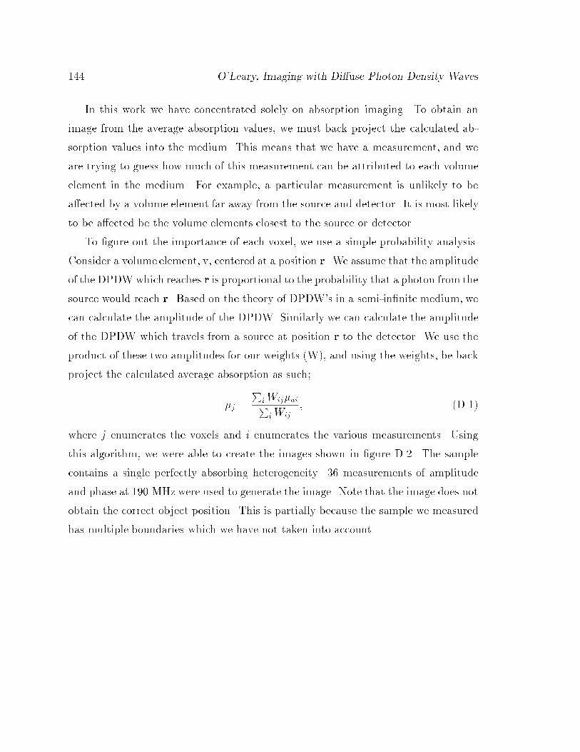
144 O'Leary, Imaging with Di�use Photon Density Waves
In this work we have concentrated solely on absorption imaging. To obtain an
image from the average absorption values, we must back project the calculated ab-
sorption values into the medium. This means that we have a measurement, and we
are trying to guess how much of this measurement can be attributed to each volume
element in the medium. For example, a particular measurement is unlikely to be
a�ected by a volume element far away from the source and detector. It is most likely
to be a�ected be the volume elements closest to the source or detector.
To �gure out the importance of each voxel, we use a simple probability analysis.
Consider a volume element, v, centered at a position r. We assume that the amplitude
of the DPDW which reaches r is proportional to the probability that a photon from the
source would reach r. Based on the theory of DPDW's in a semi-in�nite medium, we
can calculate the amplitude of the DPDW. Similarly we can calculate the amplitude
of the DPDW which travels from a source at position r to the detector. We use the
product of these two amplitudes for our weights (W), and using the weights, be back
project the calculated average absorption as such;
�j =
PiWij ��aiPiWij
; (D.1)
where j enumerates the voxels and i enumerates the various measurements. Using
this algorithm, we were able to create the images shown in �gure D.2. The sample
contains a single perfectly absorbing heterogeneity. 36 measurements of amplitude
and phase at 190 MHz were used to generate the image. Note that the image does not
obtain the correct object position. This is partially because the sample we measured
has multiple boundaries which we have not taken into account.
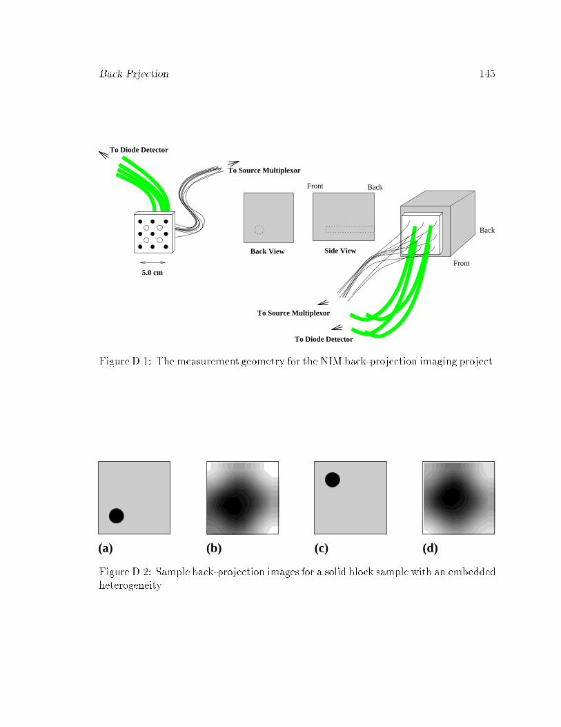
Back Prjection 145
5.0 cm
To Diode Detector
To Source Multiplexor
To Source Multiplexor
To Diode Detector
Front
Back
Side ViewBack View
Front Back
Figure D.1: The measurement geometry for the NIM back-projection imaging project.
(a) (b) (c) (d)
Figure D.2: Sample back-projection images for a solid block sample with an embedded
heterogeneity.

146 O'Leary, Imaging with Di�use Photon Density Waves
Appendix E
The Photon Migration Imaging Software Package
PMI is a general purpose program (developed by David Boas, Maureen O'Leary,
and Xingde Li at the University of Pennsylvania, and Martin Ostermeyer at the
University of Texas/ M.D. Anderson Cancer Center) for solving various forward and
inverse problems related to photon migration. The purpose of the program is to
enable researchers to explore the propagation of di�using photons through general
heterogeneous, turbid media and to derive information about such turbid media from
measurements of the di�using photons. PMI has a modular design to facilitate the
addition of new algorithms as they become available. The following modules are
currently available:
� EXACT: Various analytic solutions to the di�usion equation are used for cal-
culating the scattering of Di�use Photon Density Waves (DPDW's) from spherical
and cylindrical objects embedded in in�nite or semi-in�nite media as well as the
propagation of DPDW's in homogeneous media.
� TIME DOMAIN: This module enables calculations to generate data in the time
domain and enables time domain data to be used for the inverse problem. The forward
problem is done by doing the calculations in the frequency domain and FFT'ed to
the time domain. Experimental data in the time domain can be loaded. It is then
FFT'ed to the frequency domain for analysis.
� LAYERED: This module provides an analytic solution for a two layered, semi-
in�nite system. The source and detector are assumed to be on the air-top layer
interface. The bottom layer is displaced a user de�nable distance from the air-top
147
148 O'Leary, Imaging with Di�use Photon Density Waves
layer interface.
� FLUORESCENCE: This module contains analytic solutions for the generation
and propagation of uorescent DPDW's in media with spatially uniform and spatially
varying optical properties.
� FIT: This is a chi-squared squares �tting algorithm for analyzing experimental
or simulated data to �nd the optical properties of the background media, optical
properties of any spherical or cylindrical objects, and/or the position of any spherical
or cylindrical objects.
� RECONSTRUCTION: This program uses an iterative routine (SIRT) to solve
for the optical properties of an inhomogeneous medium. The inversion will reconstruct
absorption and/or scattering, uorescence lifetime, Brownian di�usion, or shear ow.
The theory is based on the First Born or First Rytov approximation and forward
data may be generated using these algorithms.
� MIE: This module provides commands for calculating the scattering coe�cient
and anisotropy factor of spherical dielectrics using Mie Theory. The wavelength
dependent index of refraction for water and polystyrene is included in this module.
The input is line oriented and can come either from an input �le or from the
standard input (keybord). Normally the input �le is speci�ed in the command line
when the program is started:
unixprompt> pmi [inputfilename]
The program will execute the commands in the input �le and return to the Unix
prompt. If no input �le is speci�ed, the program switches to the interactive mode
and waits at its prompt for input. Now command after command can be typed in,
or an input�le can be speci�ed with the Include command:
|PMI> Include [input file name]
After the commands in the input�le are executed, the program will return to its
prompt and wait for more commands. Any text after a # sign is taken to be a
comment.
PMI Software 149
Sample input �les (scripts) are shown below. Note that the immaging script uses
the main shell to set up the medium, etc., the exact module to calculate the forward
data, and the reconstruction module to invert the data.
E.1 Sample PMI scripts
Sample scripts to run with PMI VERSION 2.0
List of sample scripts:
* exact1.pmi - Calculates the DPDW distorted by a spherical
absorber.
* fit1.pmi - Fits data for a distorted DPDW for the position and
radius of the spherical absorber.
* image1.pmi - Creates an image of the absorption using a
reconstruction technique.
--------------------- EXACT1.PMI ---------------------
Following is a sample script to calculate the DPDW distorted by a
spherical absorber. A 200 MHz source is positioned at the origin with
an initial amplitude of 1 and phase of 0. The absorber has a radius of
0.5 cm and is centered at x=0, y=2, and z=0. The detector is scanned
from x=-4 cm to x=4 cm at y=4 cm and z=0 cm.
# The following script will using the analytic solution for the
# scattering of DPDW's from spherical objects to calculate the
# amplitude and phase of the distorted DPDW.
# Define the medium used for the background
# [name] [mua] [mus] [g] [n] [zeros]
Medium Tissue .1 10 0 1.333 0 0 0
Background Tissue
# Define the medium for the spherical inhomogeneity
# [name] [mua] [mus] [g] [n] [zeros]
Medium Tumor .5 10 0 1.333 0 0 0
150 O'Leary, Imaging with Di�use Photon Density Waves
# Define the sphere
# [obj_name] [medium_name] [x] [y] [z] [r]
ObjectSphere Tumor Tumor 0 2 0 .5
# Create the source-detector list
CreateSDList grid 1 0 0 0 1 0 200 200 1 0 0 1 -4 4.1 1 4 4 1 0 0 1
# RUN EXACT
Exact
#Save the source-detector list
# [filename]
SaveSDList foo
#Save the data list
# [FormatType] [DataType] [filename]
SaveDataList NORMAL NORMAL foo
--------------------- fit1.pmi ---------------------
Fits the data created with exact1.pmi for the x position and radius of
the absorbing sphere.
# This script includes the script exact1.pmi to calculate the
# distorted DPDW and then uses the FIT module to fit for the x
# position and radius of the sphere.
# include the exact1.pmi script
Include exact1.pmi
# set the unknown parameters
SetFitParam xo .1 .5
SetFitParam a 1 .5
# Fit for the unknown parameters
Fit
# Save the result
SaveFitResult foo DATA PARAM NOAPPEND
--------------------- image1.pmi ---------------------
PMI Software 151
Defines a set of measurements, an spherical inhomogeneity, and the
data that would be measured. Then inverts this data to solve for the
absorption as a function of position.
# this script should produce a nice image of a sphere with a max
# absorption of .00303
# mua mus g n db
DefineMedium back .03 10. 0. 1.333
DefineMedium obj .04 10. 0. 1.333
# SET UP THE GEOMETRY
background back
geometry infinite
RegionBox entire back -3.0 -3.0 -.0 3.0 3.0 .0
#for reconstruction: solve for absorption, use both amp & phase data,
# use the born approx, 1000 SIRT iterations, use the
# homogeneous Green functions
SetReconParams ABSORPTION BOTH BORN 1000 DPDW
# constrain the absorption change to be positive
SirtConstraints 0 50 0 50 0 50
# place a sphere in the medium
objectsphere test1 obj .5 -.5 0. .5
# scan around the sides of a box
CreateSDList tandem 1 3 0 0 1 0 200 200 5 0 0 .5 -3 3 .5 0 0 .5 -3 0 0
CreateSDList tandem 1 0 3 0 1 0 200 200 5 -3 3 .5 0 0 .5 0 0 .5 0 -3 0
# use the exact module to create the forward data
Exact
# subtracts the incident from the total wave - no noise added
BornData 0. 0.
# free the object list to start with a guess of zero
freeobjectlist
# set up the region to reconstruct
Initimage -4.0 4.0 .25 -4.0 4.0 .25 -.0 .0 .58
152 O'Leary, Imaging with Di�use Photon Density Waves
#create the weights
createweights
# do the first order reconstruction
runsirt
saveimage filenm
E.2 PMI Command Summary
PMI Online Help from 10 July 96
Version 2.1
-----------------------------------------------
PMI Command Groups
* General: General commands
* Programming: Script programming commands
* Sources, Detectors, and Data: Commands for manipulating sets of
sources, detectors, and data.
* Medium: Commands for defining the properties of different turbid
media.
* Boundaries: Commands for defining the boundaries of a system and
the boundary condition.
* Objects: Commands for defining inhomogeneities
* Images: Commands for manipulating Images of the optical
properties and the fluence.
Commands associated with different modules
* Exact Module: Commands related to the EXACT module. A description
of the EXACT module is found here.
* Time Domain Module: Commands related to performing calculations
in the time domain.
* Layered Media Module: Commands related to the layered media
module.
* Fluorescence Module: Commands related to the Fluorescence module.
* Fit Module: Commands related to running the FIT module.
* Reconstruction Module: Commands for reconstructing optical
properties from measurements of the fluence. A description of the
RECONSTRUCTION module is found here. Refer to the sample script
image1.pmi for an example.
PMI Software 153
* MIE Module: Commands for calculation of the scattering
coefficient and anisotropy factor of spherical dielectrics based
on Mie Theory. The wavelength dependent index of refraction for
water and polystyrene is included in this module.
---------------------------------------------------
PMI Command Summary
* General: General commands
o Include, Prompt, Interactive, System, Bell, Echo, Exit,
Quit, Help, SetHTMLhelp, SetPMIdir, Pipes
* Programming: Script programming commands
o For...Next Loops, Variables, Operations, While Blocks, If
Blocks, Functions, SetVariableVormat, Input,
PassedArguments, StringCompare
* Sources, Detectors, and Data: Commands for manipulating sets of
sources, detectors, and data.
o For automatic creation of whole SDLists: CreateSDList,
SaveSDList, SaveDataList LoadSDDList, LoadSDList,
FreeSourceList, AddNoise, AddConstantNoise Seed
o For manual creation of SDDSets: OpenNewSDDSet,
CloseNewSDDSet, AddSingleSource, AddDetectorLine,
AddDetectorPlane, AddDetectorVolume, PrintDetector
* Medium: Commands for defining the properties of different turbid
media.
o Medium, DefineMedium, DefineMediumDynamics,
DefineMediumFlourescence, PhotonDiffusion, Background,
ShowMedium, FreeMedium, RegionSphere, RegionCylinder,
RegionBox
* Boundaries: Commands for defining the boundaries of a system and
the boundary condition.
o Plane, BoxPlanes, FreePlane, BoundaryCondition, Geometry
* Objects: Commands for defining inhomogeneities
o ObjectSphere, ObjectCylinder, ObjectBox, ObjectGauss,
ApplyObjects, ShowObject, FreeObjectList
* Images: Commands for manipulating Images of the optical
properties and the fluence.
o InitImage, SaveImage, SaveDynamicImage LoadImage ,
Commands associated with different modules
* Exact Module: Commands related to the EXACT module. A description
154 O'Leary, Imaging with Di�use Photon Density Waves
of the EXACT module is found here.
o Exact, Moments, Smallest
* Time Domain Module: Commands related to performing calculations
in the time domain.
o Freq2Time, SaveTimeData, SaveTimeData_WWWStandard, TRS2TDD,
LoadTimeData
* Layered Media Module: Commands related to the layered media
module.
o Layered
* Fluorescence Module: Commands related to the Fluorescence module.
o FLR_Exact
* Fit Module: Commands related to running the FIT module.
o Fit, SaveFitResult, SetFitParam, SetFitTolerance,
SetFitMaxIter
* Reconstruction Module: Commands for reconstructing optical
properties from measurements of the fluence. A description of the
RECONSTRUCTION module is found here. Refer to the sample script
image1.pmi for an example.
o SetReconParams, NoSirtConstraints, PertData RytovData ,
BornData, CreateWeights, SaveWeights, RunSirt,
SirtConstraints, NoSirtConstraints
* MIE Module: Commands for calculation of the scattering
coefficient and anisotropy factor of spherical dielectrics based
on Mie Theory. The wavelength dependent index of refraction for
water and polystyrene is included in this module.
o Lambda, Mie, MiePoly
Examples can be found in the sample scripts. Check also the PMI
homepage.
---------------------------------------------------
PMI Command Index
* AddConstantNoise
* AddDetectorLine
* AddDetectorPlane
* AddDetectorVolume
* AddNoise
* AddSingleSource
* ApplyObjects
* Background
* Bell
PMI Software 155
* BornData
* BoundaryCondition
* BoxPlanes
* CloseNewSDDSet
* CreateSDList
* CreateWeights
* DefineMedium
* DefineMediumDynamics
* DefineMediumFlourescence
* Echo
* Exact
* Exit
* Fit
* SetFitTolerance
* FLR_Exact
* For...Next Loops
* FreeMedium
* FreeObjectList
* FreePlane
* FreeSourceList
* Freq2Time
* Functions
* Geometry
* Help
* If Blocks
* Include
* InitImage
* Input
* Interactive
* Lambda
* Layered
* LoadSDDList
* LoadSDList
* LoadTimeData
* Medium
* Mie
* MiePoly
* Moments
* NoSirtConstraints
* ObjectBox
* ObjectCylinder
* ObjectGauss
* ObjectSphere
156 O'Leary, Imaging with Di�use Photon Density Waves
* OpenNewSDDSet
* Operations
* PassedArguments
* PertData
* PhotonDiffusion
* Pipes
* Plane
* PrintDetector
* Prompt
* Quit
* RegionBox
* RegionCylinder
* RegionSphere
* RunSirt
* RytovData
* SaveDataList
* SaveDynamicImage
* SaveFitResult
* SaveImage
* SaveSDList
* SaveTimeData
* SaveTimeData_WWWstandard
* SaveWeights
* Seed
* SetFitMaxIter
* SetFitParam
* SetHTMLhelp
* SetPMIdir
* SetReconParams
* SetVariableFormat
* ShowMedium
* ShowObject
* SirtConstraints
* Smallest
* StringCompare
* System
* TRS2TDD
* Variables
* While Blocks
* LoadImage
---------------------------------------------------
PMI Software 157
Command Descriptions
---------------------------------------------------
General Commands
Following is a list of miscellaneous commands for PMI:
* Quit or Exit - to exit PMI.
* Include [filename] - Used to execute the commands in the script
given by [filename]. Included files may in turn use the Include
command. If [filename] could not be found it is searched for in
the PMI directory.
* Interactive - switches the program to the interactive mode. This
makes only sense as a command in an input file. A single point in
a line or ^d (Control d) terminates the interactive mode, the
control of the program returns to the superior file from which
the Interactive command was invoked. If the interactive mode was
already the top control level, the program terminates.
* System [unix command] or: ! [unix command] - launches a unix shell
command.
* Help [command] or ? [command]- gives help for the specified
[command] or general help if [command] is missing. Gives
HTML-help if a browser and the help file have been specified
properly with the command SetHTMLhelp, or plain text help at the
PMI-prompt otherwise.
* SetPMIdir [pmi_dir] - Sets [pmi_dir] as the PMI directory. It is
convenient to use this command in the initialization file
".pmi_init" that is executed at startup.
* SetHTMLhelp [browser] [file] - Sets the paths for a HTML-browser
(i.e. Mosaic or Netscape) which is used to display the
HTML-help-file (normally "[pmi_dir]/Help/PMI_HELP.html"). It is
convenient to use this command in the initialization file
".pmi_init" that is executed at startup.
* Bell - Rings a bell.
* Echo [text] - writes text on the screen and to the log file
* Prompt - The program waits for a "RETURN". If one types "i"
"RETURN", the program executes the Interactive command.
* Pipes - Pipes are used to control command driven external
programs i.e. plot programs like gnuplot.
o OpenPipe [id] [prog_name] - Start
+ [id] - Identifies the pipe
+ [prog_name] - Name (with path) of the program to be
158 O'Leary, Imaging with Di�use Photon Density Waves
executed
o ToPipe [id] [command] - Sends [command] to pipe [id]
o ClosePipe [id] - Closes pipe [id]
o CloseAllPipes - Closes all pipes. Normally obsolete since
all pipes are closed automatically when the program
terminates.
---------------------------------------------------
Programming Commands
Following is a list of programming commands for use in scripts:
* For... Next Loops - For Next loops can be employed in scripts to
repeat a block of commands with an incrementing variable. Up to 9
nested loops can be used.
o For [Variable Name] = [min] to [max] step [step] - Start of
the For Next loop
+ [Variable Name] - Float variable to increment.
+ [min] - Start the loop with a value of [min]
+ [max] - End the loop with the value of [max]
+ [step] - increment the value by [step]
o Next - marks the end of the For Next loop
* Variables There are two types of variables: float variables and
string variables. The name of a float variable is preceded by an
& and the name of a string variable is preceded by an
$. Following are examples of assignments:
o &musp = 10 Which gives the float variable &musp the value of
10.
o &$filename = foobar Which gives the string variable
$filename the value of foobar.
The values of these variables are used in other commands as
follows
o DefineMedium tumor 0.1 &&musp 0 1.333
o SaveDataList Normal Normal $$filename NoAppend
The format used for printing the values of these variables is set
using the SetVariableFormat command.
* Operations Mathematical operations are available. They are
addition(+), subtraction(-), multiplication(*), and
division(/). Also available are trigonometric functions (sin,
cos, tan, asin, acos, atan) and exponentials (exp). These
PMI Software 159
operations are used in variable assignments. For example:
o &musp = &&musp + 5
o &D = 2.25e10 / 3 / &&mutr
o &x = 3. * Cos 30 + 1.
o $filename = data_ + &&omega + .dat
NOTE that operations are performed from left to right. For string
variables, only the addition operation is available. Arguments
for (sin, cos, tan) are in degrees. Arguments returned by (asin,
acos, atan) are in degrees.
* While Blocks - While blocks are used as conditional loops in
scripts. There can be 9 nested while blocks.
o While [value1] [condition] [value2] - Start of the While
Block.
+ [value1] and [value2] are the values being compared.
+ [condition] - Six conditions are supported: less than
(<), less than or equal to (<=), greater than (>),
greater than or equal to (>=), equal to (=), and not
equal to (!=).
o Wend - End the While Block.
* IF Blocks - If blocks are used to execute a set of commands
depending on the result of a condition. There is no limit to the
number of nested If Blocks.
o If [value1] [condition] [value2] - Start of the If Block.
+ [value1] and [value2] are the values being compared.
+ [condition] - Five conditions are supported: less than
(<), less than or equal to (<=), greater than (>),
greater than or equal to (>=), equal to (=), and not
equal to (!=).
o IfEnd - End the If Block.
* Functions - Certain commands are capable of returning values to
variables in the script, e.g. FIT. The usage is:
o COMMAND [parameters] -> &1 &2... The -> indicates that the
COMMAND will return values to the variables &1 &2.... The number
of values returned depends on the COMMAND.
* SetVariableFormat [name] [format] - Used to set the format for
printing string and float variables.
o [name] is the name of a string or float variable. Remember
to precede the string (float) variable with a $ (&).
o [format] is the format string. Standard-C format strings are
used. Therefore, string variables must have a string format
and float variables must have a float format. %s and %f are
the default formats for string and float variables
respectively.
160 O'Leary, Imaging with Di�use Photon Density Waves
* Input [variable_name] [text string] - Used to get input from the
user and place the result in a variable. For example,
o Input &musp What is the reduced scattering coef.?
* PassedArguments [var1] [var2]... - Used if arguments are passed
to an included file. There are two ways to pass arguments to an
include file: from the unix prompt you follow the format
o unixprompt> pmi [include_file] [var1] [var2] ... or from
the PMI interactive mode
o |PMI> Include [include_file] [var1] [var2] ... The
arguments are then passed to variables in the include file by
using this command in the include file. PassedArguments can be
used anywhere in the include file and can be used any number of
times. For example, if you have an include file that expects musp
and mua to be passed as arguments, then include the following
line at the top of the include file:
o PassedArguments &musp &mua The float variable &argc is set
equal to the number of passed arguments when a new script is
included.
* StringCompare [var1] = [var2] - This FUNCTION does a string
compare. It returns 0 if the strings are equal and 1 if they are
not equal. The compare is not case sensitive. Example:
o StringCompare $$FitWhat = MUSP -> &result
---------------------------------------------------
Object Commands
The following commands are used for defining different
inhomogeneities:
* ObjectSphere [name] [medium] [x] [y] [z] [r] - Used to define a
spherical inhomogeneity.
o [name] - is the name of the sphere. The name may be
exploited in future versions of PMI.
o [medium] - is the name of the medium which fills the sphere,
e.g. tumor or hematoma. The medium must be defined prior to
execution of ObjectSphere using the command DefineMedium
o [x] [y] [z] - define the position of the center of the
sphere with units of cm.
o [r] - is the radius of the sphere in units of cm.
* ObjectCylinder [name] [medium] [x1] [y1] [z1] [x2] [y2] [z2] [r]
- Used to define a cylindrical inhomogeneity.
o [name] - is the name of the cylinder. The name may be
PMI Software 161
exploited in future versions of PMI.
o [medium] - is the name of the medium, see in ObjectSphere.
o [x1] [y1] [z1] - defines the position of the center of the
bottom of the cylinder (units of cm).
o [x2] [y2] [z2] - defines the position of the center of the
top of the cylinder (units of cm). Note that EXACT can only
work with infinite cylinders and thus only uses these
positions to define the axis of the cylinder. Presently,
EXACT can only work with cylinders which have an axis
parallel to the z-axis.
o [r] - is the radius of the cylinder (units of cm).
* ObjectBox [name] [medium] [xlo] [ylo] [zlo] [xhi] [yhi] [zhi] -
Used to define a rectangular inhomogeneity with sides parallel to
the coordinate axes.
o [name] - is the name of the box. The name may be exploited
in future versions of PMI.
o [medium] - is the name of the medium, see in ObjectSphere.
o [xlo] [ylo] [zlo] - define the lower x, y, z values (units
of cm).
o [xhi] [yhi] [zhi] - define the upper x, y, z values (units
of cm).
---------------------------------------------------
Medium Commands
The following commands are used to define the properties of different
media:
* Medium - THIS COMMAND IS OBSOLETE. Use DefineMedium instead.
* DefineMedium [name] [mua] [mus] [g] [n] - Used to define or
change the properties of a medium.
o [name] - is the name of the medium which is used by other
parts of the program to reference a particular medium.
o [mua] - is the absorption coefficient of the medium.
o [mus] - is the scattering coefficient of the medium.
o [g] - is the average cosine of the scattering angle.
o [n] - is the index of refraction.
* DefineMediumDynamics [name] [Brownian] [Shear] - Used to define
or change the DYNAMICAL properties of a medium.
o [name] - is the name of the medium which is used by other
parts of the program to reference a particular medium.
o [Brownian] - is the Brownian diffusion coefficient of the
scattering particles in units of cm^2/s.
162 O'Leary, Imaging with Di�use Photon Density Waves
o [Shear] - is the rate of shear for the scattering particles
in units of 1/s.
* DefineMediumFluorescence [name] [tau] [mua_f] [musp_f] [fmua]
[fmusp] [fmua_f] [fmusp_f] - Used to define or change the
FLUORESCENT properties of a medium.
o [name] - is the name of the medium which is used by other
parts of the program to reference a particular medium.
o [tau] - is the fluorescence lifetime.
o [mua_f] - is the absorption coefficient of the chromophore
at the fluorescence wavelength.
o [musp_f] - is the reduced scattering coefficient of the
chromophore at the fluorescence wavelength.
o [fmua] - is the absorption coefficient of the fluorophore at
the excitation wavelength.
o [fmusp] - is the reduced scattering coefficient of the
fluorophore at the excitation wavelength.
o [fmua_f] - is the absorption coefficient of the fluorophore
at the fluorescence wavelength.
o [fmusp_f] - is the reduced scattering coefficient of the
fluorophore at the fluorescence wavelength.
* Background [medium_name] - Used to set the background medium.
o [medium_name] - is the name of the medium defined using the
DefineMedium command.
---------------------------------------------------
Sources and detectors
Several sources, each with its own amplitude and phase, and several
detectors, also with amplitude and phase, are organized in a
Source-Detector-Data-Set (SDDS). The modulation frequency and the
correlation time are the same for a SDDSet and all sources are 'on' at
the same time. The forward algorithms (Exact andPertData) can operate
on one SDDSet at a time. If one wants to calculate situations with
several modulation frequencies or correlation times or with changed
source or detector positions, one has to create several SDDSets. All
the SDDSets are stored in a list, the SDList.
Because inverse algorithms work with the SDList there is a group of
commands for creating, saving, and loading a whole SDList as well as
saving and loading the corresponding data in one step. For pure
forward calculations it can be more convenient to set a SDDSet 'by
hand', which is done by the second group of commands.
Commands for SDLists
PMI Software 163
* CreateSDList [format] [parameters...] - Used to create a
source-detector set.
o [format]=GRID This format is used to create a set of
detectors for a spatially fixed source group. The modulation
frequency and correlation time of the source can be scanned
as well as the X, Y, and Z coordinates of the detector.
+ [parameters...] =
+ [number of Sources in Source Group]
+ [Xs] [Ys] [Zs] [Amp] [Ph] ... Position and initial
amplitude and phase of each source in the source group.
+ [Omega Min] [Omega Max] [Omega Step] Frequency given in
Mhz
+ [Tau Min] [Tau Max] [Tau Step] Correlation time in
seconds
+ [X Min] [X Max] [X Step] X coordinates of the detector
+ [Y Min] [Y Max] [Y Step] Y coordinates of the detector
+ [Z Min] [Z Max] [Z Step] Z coordinates of the detector
o [format]=TANDEM This format is used to scan a source group
and detector in tandem. A grid is defined and the position
of the source group and detector are given relative to the
grid points.
+ [parameters...] =
+ [number of Sources in Source Group]
+ [Xs] [Ys] [Zs] [Amp] [Ph] ... Position and initial
amplitude and phase of each source in the source
group. The position is given relative to the grid
points defined below.
+ [Omega Min] [Omega Max] [Omega Step] Frequency given in
Mhz
+ [X Min] [X Max] [X Step] X coordinates of the grid
points
+ [Y Min] [Y Max] [Y Step] Y coordinates of the grid
points
+ [Z Min] [Z Max] [Z Step] Z coordinates of the grid
points
+ [X det] [Y det] [Z det] Position of the detector
relative to the grid points
o [format]=CYLINDER2 This format is used to scan a source and
scan a detector around a cylinder. A grid is defined and the
position of the source group is given relative to the grid
points. Next a detector grid is defined relative to the
source grid points. Thus, for each source there are a grid
of detectors.
164 O'Leary, Imaging with Di�use Photon Density Waves
+ [parameters...] =
+ [Zmin] [Zmax] [Zstep] The z positions for the source
grid.
+ [Phis_Min] [Phis_Max] [Phis_Step] The phi positions for
the source grid.
+ [rho] This is the radius of the cylindrical scan.
+ [omega] Modulation frequency
+ [tau] Correlation time
+ [Num_Srcs] number of sources in the source group
+ [Zsrc] [Phi_src] [Amp] [Ph] ... Position and initial
amplitude and phase of each source in the source
group. The position is given relative to the source
grid points.
+ [Z_det] [Phi_Min_Det] [Phi_Max_Det] [Phi_Step_Det]
Definition of the detector grid relative to the source
grid.
o [format]=TDTANDEM This format is used to define a pulsed
source. The source and detector are scanned in tandem on a
grid. The source and detector positions are defined relative
to the grid.
+ [parameters...] =
+ [xmin] - define the x part of the grid
+ [xmax]
+ [xstep]
+ [ymin] - define the y part of the grid
+ [ymax]
+ [ystep]
+ [zmin] - define the z part of the grid
+ [zmax]
+ [zstep]
+ [xsource]- Separation between grid point and source
+ [ysource]
+ [zsource]
+ [amp] - Initial amplitude of source
+ [ph] - Initial phase of source
+ [xdetectr] - Separation between grid point and
detector
+ [ydetector]
+ [zdetector]
+ [tmax] - Amount of time to watch the response to a
pulse at time = 0. Units of seconds. This sets the
frequency step, i.e. freq. step = 1/[tmax].
+ [number bins] - Number of bins to divide [tmax] in
PMI Software 165
to. Must be a power of 2.
+ [freq max] - Maximum frequency for calculations. Units
of MHz. If this is too small then oscillations will
appear in the time domain data as artifacts.
* SaveSDList [filename] - Used to save a list of source-detector
sets
o [filename] - is the filename for the output file. Note that
.sd is appended to the filename
* SaveDataList [FormatType] [DataType] [filename] [append] - Used
to save a list of data.
o [FormatType] One of the following:
+ Normal - creates a data file with the standard PMI code
format. [DataType] can have the following values:
+ Normal - saves the incident and total amplitude
and phase.
+ Total/Incident - saves the ratio of the total to
the incident.
+ WWWstandard - uses the format designed for sharing data
over the WWW. [DataType] can have the following values:
+ Normal - saves the incident and total amplitude
and phase.
o [DataType] - determines what type of data is saved,
e.g. save the total amplitude and phase or relative to the
incident amplitude and phase. The value of this parameter
depends on the chosen [FormatType].
o [filename] - is the filename for the output file. Note that
.dat is appended to the filename
o [append] - if this equals APPEND then the output is appended
to [filename]
* AddNoise [shot noise] [position uncertainty] - Used to add noise
to a set of data.
o [shot noise] - When this is not equal to zero then shot
noise is added to the data, The noise is determined by
taking the square-root of the fluence multiplied by [shot
noise]. [shot noise] is thus the product of the source
amplitude in units of photons per second, the signal
integration time in units of seconds, the detector area in
units of cm^2, and the quantum efficiency of the detector.
o [position uncertainty] - When this is not equal to zero then
random noise is added to the data as given by the
uncertainty of the position of the source and/or detector
relative to each other and/or relative to the
sample. [position uncertainty] is given in units of cm.
166 O'Leary, Imaging with Di�use Photon Density Waves
* AddConstantNoise [amp error] [phase error] - Used to add CONSTANT
noise to a set of data. [amp error] is given as a
percentage. [phase error is given in degrees.
* Seed [integer] - Used to seed the random number generator. Use
large negative integers.
Commands for individual SDDSets
* OpenNewSDDSet [name] [f] [tau] - Used to create a new SDDSet with
the identification [name], the modulation frequency [f] in Hz,
and the correlation time [tau] in seconds. After this command
sources and detectors can be added until the SDDSet is closed
with CloseNewSDDSet.
* CloseNewSDDSet [name] - Used to close the SDDSet with the name
[name].
* AddSingleSource [amplitude] [phase] [x] [y] [z] - Adds a source
to the currently open SDDSet.
o [amplitude] in W
o [phase] in degree
o [x] [y] [z] position in cm
* AddDetectorLine [name] [amp] [ph] [x] [y] [z] [e1x] [e1y] [e1z]
[lo1] [hi1] [step1] - Adds a line of detectors with arbitrary
orientation to the currently open SDDSet.
o [amp] [ph] amplitude and phase for the whole line.
o [x] [y] [z] position
o [e1x] [e1y] [e1z] vector that specifies the direction of the
line, starting from (x,y,z).
o [lo1] [hi1] [step1] specifies distribution of detectors
along the line. The zero of the coordinate system is at
(x,y,z), the direction is specified by the vector e1.
* AddDetectorPlane [name] [amp] [ph] [x] [y] [z] [e1x] [e1y] [e1z]
[lo1] [hi1] [step1] [e2x] [e2y] [e2z] [lo2] [hi2] [step2] - Adds
a plane of detectors with arbitrary orientation to the currently
open SDDSet.
o [amp] [ph] amplitude and phase for the whole plane.
o [x] [y] [z] position of the origin of the new coordinate
system.
o [e1x] [e1y] [e1z] and [e2x] [e2y] [e2z] are two vectors e1
and e2 that specify the axes of the new coordinate
system. The zero of the new coordinate system is at (x,y,z).
o [lo1] [hi1] [step1] and [lo2] [hi2] [step2] specify the
sampling along the axes of the coordinate system. The zero
of the coordinate system .
* AddDetectorVolume [name] [amp] [ph] [x] [y] [z] [e1x] [e1y] [e1z]
[lo1] [hi1] [step1] [e2x] [e2y] [e2z] [lo2] [hi2] [step2] [e3x]
PMI Software 167
[e3y] [e3z] [lo3] [hi3] [step3] - Adds a rectangular volume of
detectors with arbitrary orientation to the currently open
SDDSet. Syntax similar to AddDetectorPlane but with an additional
vector e3.
* PrintDetector [name] [printwhat] [style] [filename] - Writes
values at detectors.
o [name] name of a detector that was defined with
AddDetectorLine or AddDetectorPlane.
o [printwhat] ... sorry, no complete description yet, some of
many choices are:
+ AM_P - amplitude of perturbation fluence
+ PH_P - phase of perturbation fluence
+ AM_F - amplitude of total fluence
+ PH_F - phase of total fluence
+ AM_B - amplitude of background fluence
+ PH_B - phase of background fluence
+ PH_DIF - phase difference between total and background
fluence
+ AM_RAT - amplitude ratio between total and background
fluence
o [style] can be one of the following:
+ GNU - file can be plotted directly with gnuplot.
+ MATH - file can be plotted directly with
Mathematica. In Mathematica type: <<filename
o [filename] specifies the file. If no filename is given,
PrintDetector writes on the screen.
---------------------------------------------------
IMAGE module commands
The following commands are used for defining the image matrix of a
finite system. Each voxel in the image contains the optical properties
defined by the user by setting the background medium and the object
list.
* InitImage [X min] [X max] [X step] [Y min] [Y max] [Y step] [Z
min] [Z max] [Z step] - sets area to be considered. The area to
be reconstructed should be a subset of this large cube. The
corners on the cube and the step define the region. When
InitImage is called, then optical properties of any objects which
have been defined are inserted (voxel by voxel) into the image.
* SaveImage [filename] [parameters] - save an image to the file
filename. The format of the image file is as follows:
o [number of x] [number of y] [number of z]
168 O'Leary, Imaging with Di�use Photon Density Waves
o [xmin] [xmax] [xstep]
o [ymin] [ymax] [ystep]
o [zmin] [zmax] [zstep]
o a list of the quantities that have been saved
o the background parameters for each or these quantities
Next, the columns of data are listed. The valid parameters are
scattering (MUSP), absorption (MUA), index of refraction (N),
Browninan diffusion (DB), and shear (SHEAR). If NOHEADER is
included in the parameter list, then the first 6 rows are
omitted. Note: You cannot use LoadImage to read in a saved image
if it is saved with the NOHEADER option.
* LoadImage [filename] - read a previously saved image into
memory. The image CANNOT have been saved with the headers
disabled.
---------------------------------------------------
BOUNDARY module commands
The following commands are used for defining the boundaries of a
finite system and the boundary condition to be used in the
calculations.
* Plane [a] [b] [c] [d] [n out] - Used to define a planar boundary.
o [a] [b] [c] [d] - The plane is defined by the equation [a] X
+ [b] Y + [c] Z + [d] = 0. Note that [a] [b] [c] is the
normal vector to the plane and must point towards the turbid
medium.
o [n out] - is the index of refraction on the free-space side
of the planar boundary.
* BoxPlanes [x1] [y1] [x2] [y2] - Used to define a BOX
geometry. The sides of the box are assumed parallel to the XZ and
YZ planes. Opposite corners of the box in the XY plane are given
by [x1] [y1] and [x2] [y2]. Note that [x1] [y1] must be less than
[x2] [y2]. The geometry type is automatically set to BOX.
* BoundaryCondition [parameter] - Used to define the boundary
condition. [parameter] is one of the following:
o Zero - uses the zero boundary condition in calculations.
o Extrapolated - uses the extrapolated boundary condition in
calculations.
* Geometry [parameter] - Used to set the geometry type as given by
[parameter]. [parameter] is one of the following:
o Infinite - Calculations are performed for an INFINITE
PMI Software 169
medium.
o Planar - for a medium with PLANAR boundaries.
o Box - for a medium with BOX boundaries.
---------------------------------------------------
EXACT module commands
These commands will calculate the incident, scattered, and total
fluence for the system defined using object, medium, and boundary
commands.
* Exact - Used to calculate the analytic solution of the diffusion
equation for the defined system.
* Moments [file name] [number of moments] - Used to tell EXACT how
many moments to save to file name [file name] during the
calculation of the scattered wave. If [number of moments] is
negative then the moments are appended to the file.
---------------------------------------------------
TIME-DOMAIN module commands
These commands are used to perform calculations in the time-domain. It
is necessary to prepare the program for time-domain calculations
either by creating pulsed sources with CreateSDList or by loading a
time-domain set of data with LoadTimeDomain.
* Freq2Time - All calculations are done in the
frequency-domain. After the calculations, it is necessary to tell
the program to Fourier transform the results into the
time-domain. This is done with Freq2Time. There are no
parameters. This will only work if a pulsed source has been
defined with CreateSDList or a time-domain data set was loaded
with LoadTimeDomain.
* SaveTimeData [Format Type] [Data Type] [File name] [Append] -
Used to save time-domain data to file [File name].
o [FormatType] One of the following:
+ Standard - Creates a data file with the standard PMI
code format. [DataType] is not used.
+ Time - Saves the data in two column format. The first
column is the time in nanoseconds and the second column
is the fluence. [DataType] is not used.
170 O'Leary, Imaging with Di�use Photon Density Waves
o [DataType] - Not used, however you must place a word
here. Use foo if you can't think of anything else.
o [filename] - is the filename for the output file. Note that
.tdd is appended to the filename
o [append] - if this equals APPEND then the output is appended
to [filename]
* SaveTimeData_WWWStandard - Don't use.
* TRS2TDD [File TRS] [File TDD] [nbins] [fbin] [tmax] [fmax] [xs]
[ys] [zs] [xd] [yd] [zd] - Reads in one column time-domain data
and saves it in the standard time-domain format. The first row of
the one column data file must be the number of data points that
follow in the subsequent rows.
o [File TRS] - This is name of the one column time-domain data
file. A .trs is appended to the file name. The first row
must be the number of data points that follow in the
subsequent rows.
o [File TDD] - This is file name used to save the data in the
standard .tdd format. A .tdd is appended to the file name.
o [nbins] - This is the number of data points to take from the
.trs file and save in the .tdd file.
o [fbin] - This is the first data point to take from the .trs
file. The next [nbins]-1 data points are saved as
well. This option allows initial zeros or other data sets to
be skipped.
o [tmax] - Since time information is not contained in the .trs
file it is necessary to indicate the time range spanned by
the [nbins] data points.
o [fmax] - This is the maximum modulation frequency calculated
when the Fourier transform of this data set is taken.
o [xs] [ys] [zs] - Position of the source.
o [xd] [yd] [zd] - Position of the detector.
* LoadTimeData [TDD file] [reverse] [Instrument function] - This
command will load time-domain data that is in the standard format
and deconvolute the data if an instrument function is given.
o [TDD file] - This is the .tdd file. A .tdd is appended to
[TDD file].
o [reverse] - The .tdd file must have the data in an
increasing time sequence. That is the first data point is at
time=0 and the last data point is at time=[tmax]. Some data
files are saved in the reverse format. This is indicated by
typing REVERSE here. If the data is in the proper sequence
then type NORMAL.
o [Instrument function] - This is the file containing the
PMI Software 171
instrument function. A .inst is appended to the file
name. The format is single column with the first row
containing the number of data points following in the
subsequent rows. The deconvolution of the data only works if
the [TDD file] and [Instrument function] have the same
number of data points. The time scale of the instrument
function is assumed to be the same as the data.
---------------------------------------------------
Layered module commands
These commands are used to calculate diffuse back reflection from a
layered, turbid system. Analytic solutions of the diffusion equation
are used.
* Layered [Medium 1] [Medium 2] [d] - This is the command to start
the calculation. The source-detector geometry must be defined
before calling this command. The layered medium is semi-infinite
with the free-space interface at z=0 in the xy-plane. NOTE that
the z coordinates of the sources and detectors are assumed to be
zero. It does not matter if you defined them as something other
than zero. The index of refraction outside of the turbid media is
assumed to be 1.0.
o [Medium 1] is the medium for the top layer.
o [Medium 2] is the medium for the bottom layer.
o [d] - The top layer has a thickness of [d] cm.
---------------------------------------------------
FLUORESCENCE module commands
These commands will calculate the incident, scattered, and total
FLUORESCENT fluence for the system defined using object, medium, and
boundary commands.
* FLR_Exact - Used to calculate the analytic solution of the
diffusion equation for the defined FLUORESCENT system.
---------------------------------------------------
FIT module commands
Commands for fitting analytic solutions to experimental or simulated
data follow:
172 O'Leary, Imaging with Di�use Photon Density Waves
* Fit [FitWhat] - Used to initiate the fit. The source-detector
list and data must already be defined as well as all parameters
which are known. Refer to the sample scripts for an example. This
command is a function. It returns the chi-squared value for the
fit followed by the best fit for the fit parameters. The ordering
for the returned fit parameters is given by the list in
SetFitParam.
o [FitWhat] - determines whether to fit the amplitude data
(AMP), the phase data (PHASE), or both amplitude and phase
(BOTH). For Example, Fit AMP or Fit PHASE or Fit BOTH
* SaveFitResult [filename] [DataFlag] [ParamFlag] [AppendFlag] -
Saves the results from the Fit command. Typically, the results of
the fit are written as the first line of the output file followed
by a comparison of the "experimental" and simulated data. Each
line of the data corresponds to a single source-detector pair.
o [filename] is the filename. An extension is added to
[filename] indicating what parameters where fitted.
o [DataFlag] determines what type of data is saved if any.
[DataFlag] can have the following parameters:
+ NODATA - no data is saved.
+ FREQ - each line of the data begins with the modulation
freq. in MHz of the source for that measurement.
o [ParamFlag] determines if the fitted parameters are saved to
the file. If [ParamFlag]=NOPARAM then no parameters are
saved.
o [AppendFlag] determines if the new data starts a new file or
is appended to the end of an existing file. If
[AppendFlag]=APPEND then the data is appended to the
existing file.
* SetFitParam [parameter] [value] [uncertainty] - Used to set the
initial guess and uncertainty of an unknown parameter. If you
wish to make an unknown parameter known then set the
[uncertainty] equal to zero.
o [parameter] - is one of the following
+ Xo - x position of the object center
+ Yo - y position of the object center
+ Zo - z position of the object center
+ a - radius of the object
+ musp_obj - scattering coefficient of the object
+ mua_obj - absorption coefficient of the object
+ db_obj - Brownian diffusion coefficient of the object
+ musp_back - scattering coefficient of the background
+ mua_back - absorption coefficient of the background
PMI Software 173
+ db_back - Brownian diffusion coefficient of the
background
+ musp_f_back- scattering coefficient at emission
wavelength due to chromophore
+ mua_f_back- absorption coefficient at emission
wavelength due to chromophore
+ fmusp_f_back- scattering coefficient at emission
wavelength due to fluorophore
+ fmua_f_back- absorption coefficient at emission
wavelength due to fluorophore
+ fmusp_back - scattering coefficient at excitation
wavelength due to fluorophore
+ fmua_back - absorption coefficient at excitation
wavelength due to fluorophore
+ tau_f_back - lifetime of fluorophore
o [value] - is the initial guess for the unknown parameter
o [uncertainty] - is an estimate of the uncertainty in the
initial guess
* SetFitTolerance [tolerance] - Used to set the tolerance that
must be met when using the FIT module to determine unknown
parameters.
* SetFitMaxIter [max] - Used to set the maximum number of
iterations for the AMOEBA fit.
---------------------------------------------------
Reconstruction module commands
The reconstruction module inverts the first order solution to the
integral equation using either the Born or Rytov Expansion (see Kak
and Slaney for descriptions of the Born and Rytov expansions for
diffracting sources). The user must define the quantities to be
inverted (i.e. absorption, scattering), the grid to reconstruct on,
and the measurement geometry. The only inversion available here is the
SIRT algorithm. Refer to the sample script image1.pmi for an example.
* SetReconParams [Quantity] [Data Type] [Inverse Method]
[Iterations] [Forward Method] - sets up the reconstruction.
o [Quantity] - can be Absorption or Scattering or Both or
Brownian or Shear.
o [Data Type] - can be Amplitude or Phase or Both.
o [Inverse Method] - can be Born or Rytov.
o [Iterations] - the number of SIRT iterations.
o [Forward Method] - can be DPDW to calculate the green's
174 O'Leary, Imaging with Di�use Photon Density Waves
function for a homogeneous medium, or exact to use the exact
calculation for a sphere or cylinder, Note: exact uses the
current object list to determine what homogeneities are
present.
* RytovData [shot noise] [positional error] - divides the total
measured wave by the incident and takes the log of the
results. This is for the Rytov-type inversion. Shot noise and
positional error are added to the measurement before the
division.
* BornData [shot noise] [positional error] - subtracts the incident
wave from the total measured wave. This is for the Born-type
inversion. Shot noise and positional error are added to the
measurement before the subtraction.
* CreateWeights - uses either the Born or the Rytov approximation
to calculate the weights (also called photon hitting densities,
or three point green's functions) to necessary for the inversion
routines. WARNING: You must have a source-detector list and an
image matrix to create the weights.
* SaveWeights [filename] - saves the weights to a file. This
routine is only recommended for debugging purposes as the weight
matrix is generally quite large.
* PertData [filename] - Multiplies the weights by the image to
calculate first order forward data. The data is written to
filename.pert.dat. If filename = none, then the data is saved in
the internal source-detector-data list for further use. WARNING:
the weights and the image matrix have to have been created before
PertData is called.
* RunSirt [flag] - starts the iterative reconstruction routine. See
Kak and Slaney for details on SIRT. If the flag is set to be
CALC_WEIGHTS, then the weights are created before SIRT is
started.
* SirtConstraints [abs. min] [abs. max] [scat min] [scat. max]
[lifetime min] [lifetime max] [Brownian min] [Brownian max]
[shearmin] [shear max] - constrains the SIRT solutions for each
voxel to be between some minimum and maximum values. The
reconstruction quantities that may be constrained are absorption,
scattering, fluorescence lifetime, Brownian diffusion, and shear
flow.
* NoSirtConstraints - removes any/all constraints on reconstruction
quantities.
---------------------------------------------------
PMI Software 175
MIE module Commands
This command will calculate the l* (random walk step), which is in
another word the reciprocal of the scattering coefficient mus' for
polystyrene spheres based on Mie Theory. It requires to get the
wavelength Lambda first in the units of cm. Then either one of the
following commands can be chosen depending upon the situation. A
sample script can be found script mie.pmi.
* Lambda [wavelength] - Set the wavelength of light where
[wavelength] is in units of cm.
* Mie [param] - Used to calculate the l* (cm) given the
indices of refraction of the polystyrene spheres and the solvent,
the diameter of the polystyrene sphere (um), and the volume
fraction of polystyrene spheres in the solvent.
* MiePoly [param] -Used to calculate the l* (cm) if the
solvent is water, given the temperature (K), the diameter of the
polystyrene sphere (um), and the volume fraction of polystyrene
spheres in the solvent.
Incorporating with other PMI commands, you can use the returned value
(l*) and take advantage of the For...Next command. For details, please
see Functions for the usage of returned values and For...Next for the
loops.
---------------------------------------------------
REFERENCES
* D. A. Boas, M. A. O'Leary, B. Chance, and A. G. Yodh, Proc. Natl.
Acad. Sci. USA, 91, 4887 (1994).
* A. C. Kak and M. Slaney, Principles of Computerized Tomographic
Imaging, (IEEE Press, New York, 1988).
* M. A. O'Leary, D. A. Boas, B. Chance, and A. G. Yodh, Optics
Letters, 20(5) (1995).

176 O'Leary, Imaging with Di�use Photon Density Waves
Appendix F
Parallel Processing
There are two very di�erent methods of creating parallel code. The traditional
method, employed by Cray computers, created parallel operations (addition, multi-
plication, etc.). Parallel operations are extremely useful in large matrix calculations.
Instead of making these small operations parallel, we could make large routines paral-
lel. In this type of parallel processing, we break up a problem into large, independent
jobs, and run them each on a separate processor.
In our code we often simulate the measurements that would result from particular
source and detector. Whenever we make more than one measurement, we end up with
a set of source-detector pairs. These sets are stored internally as a list of simulations
to do. Traditionally, the code would cycle through the list, and return a corresponding
list of simulated measurements. In the new parallel code, the source-detector list is
broken up, and sections of the list are sent to multiple parallel processors.
The computer system we use for parallel processing is an IBM SP2 (Scalable
POWER Parallel2) system. POWER stands for performance optimized with en-
hanced RISC; RISC stands for reduced instruction set computer. A SP2 consists of
a series of racks of nodes. Each node is a separate RISC 6000 superscalar processor.
Nodes come in two avors. The thin nodes have a 64kB cache, and the thick nodes
have a 256kB cache. A rack consists of either 8 thick or 16 thin nodes. The system
we used had one rack consisting of 16 thin nodes.
In order to communicate between the di�erent nodes, we need a common language.
For this work we used the IBM message passing library (MPL). Since there is no
177
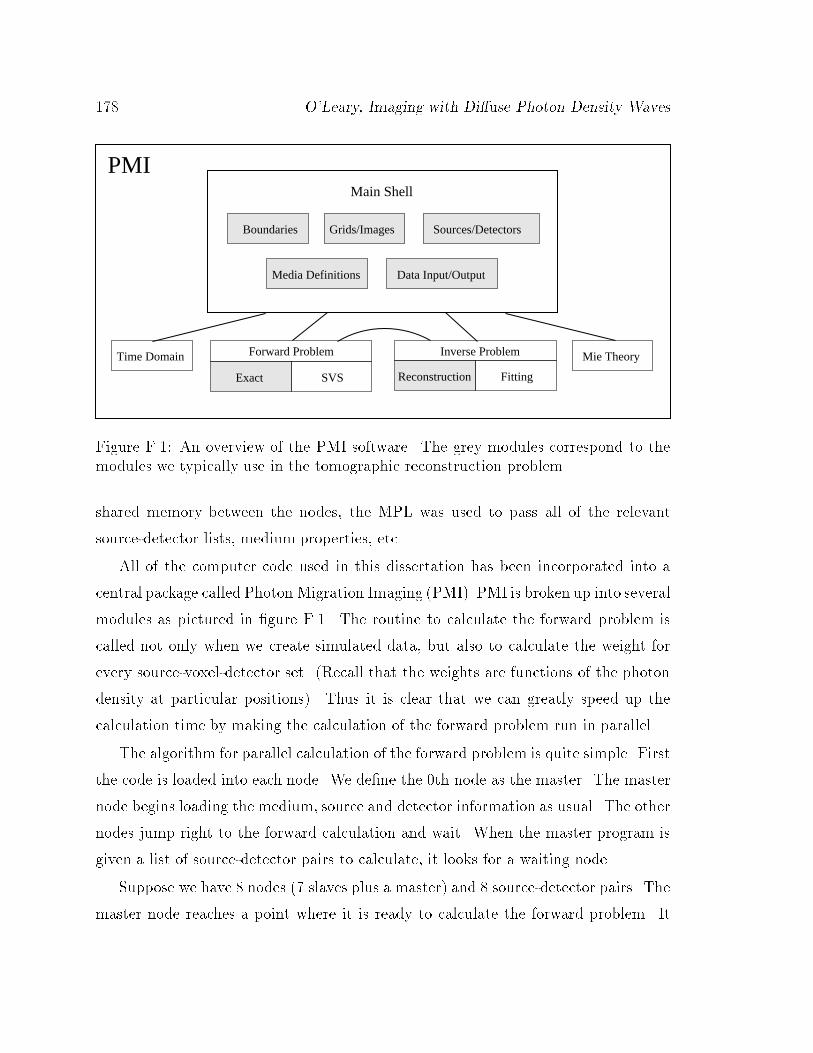
178 O'Leary, Imaging with Di�use Photon Density Waves
Inverse ProblemForward Problem
Exact
Time Domain
SVS Fitting
Grids/Images
Reconstruction
Sources/Detectors
Mie Theory
Data Input/Output
Boundaries
Media Definitions
PMIMain Shell
Figure F.1: An overview of the PMI software. The grey modules correspond to themodules we typically use in the tomographic reconstruction problem.
shared memory between the nodes, the MPL was used to pass all of the relevant
source-detector lists, medium properties, etc.
All of the computer code used in this dissertation has been incorporated into a
central package called Photon Migration Imaging (PMI). PMI is broken up into several
modules as pictured in �gure F.1. The routine to calculate the forward problem is
called not only when we create simulated data, but also to calculate the weight for
every source-voxel-detector set. (Recall that the weights are functions of the photon
density at particular positions). Thus it is clear that we can greatly speed up the
calculation time by making the calculation of the forward problem run in parallel.
The algorithm for parallel calculation of the forward problem is quite simple. First
the code is loaded into each node. We de�ne the 0th node as the master. The master
node begins loading the medium, source and detector information as usual. The other
nodes jump right to the forward calculation and wait. When the master program is
given a list of source-detector pairs to calculate, it looks for a waiting node.
Suppose we have 8 nodes (7 slaves plus a master) and 8 source-detector pairs. The
master node reaches a point where it is ready to calculate the forward problem. It
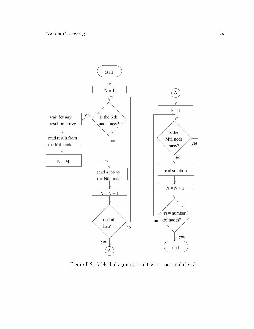
Parallel Processing 179
read result from
the Mth node
wait for any
result to arrive
N = 1
N = N + 1
Is the Nth
node busy?
end of
list?
N = M
A
Is the
busy?
Mth node
Start
A
N = 1
read solution
N = N + 1
N = number
of nodes?
end
send a job to
the Nth node
yes
no
yes
no
no
yes
no
yes
Figure F.2: A block diagram of the ow of the parallel code.
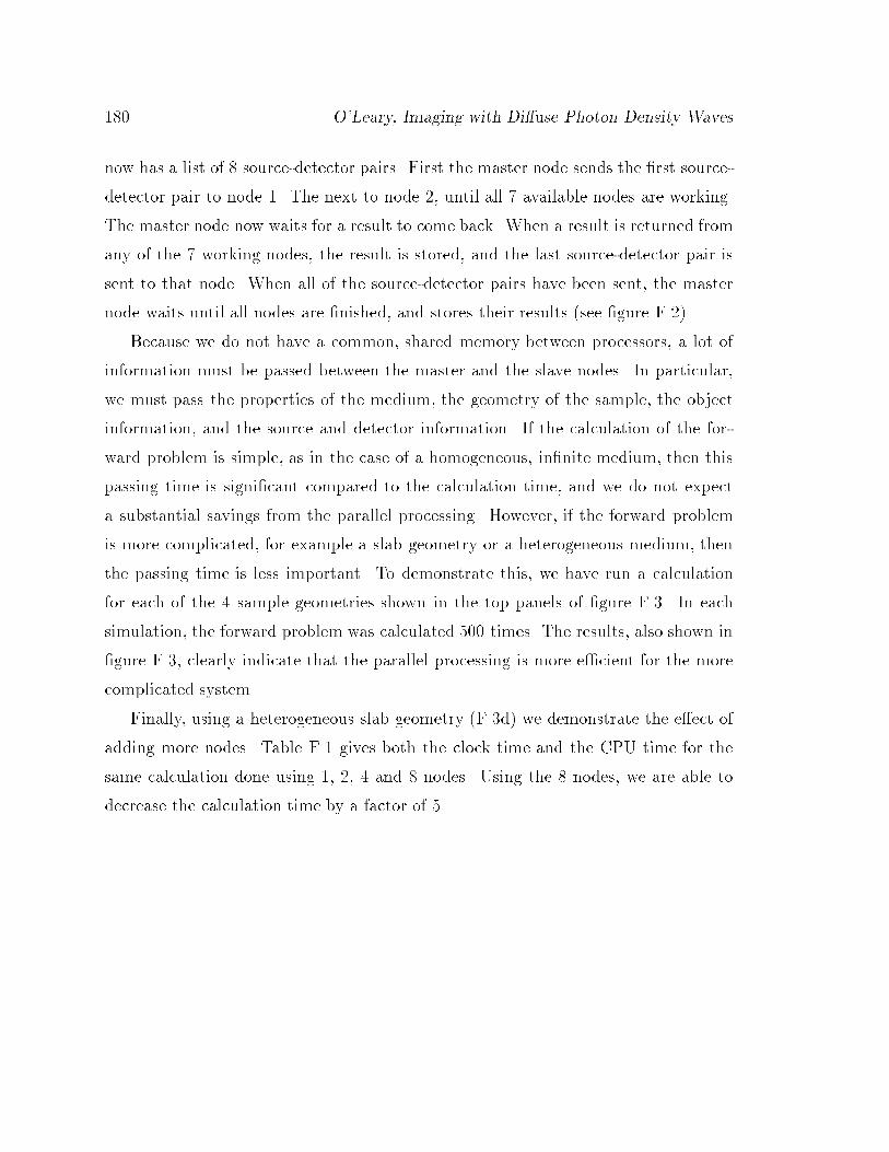
180 O'Leary, Imaging with Di�use Photon Density Waves
now has a list of 8 source-detector pairs. First the master node sends the �rst source-
detector pair to node 1. The next to node 2, until all 7 available nodes are working.
The master node now waits for a result to come back. When a result is returned from
any of the 7 working nodes, the result is stored, and the last source-detector pair is
sent to that node. When all of the source-detector pairs have been sent, the master
node waits until all nodes are �nished, and stores their results (see �gure F.2).
Because we do not have a common, shared memory between processors, a lot of
information must be passed between the master and the slave nodes. In particular,
we must pass the properties of the medium, the geometry of the sample, the object
information, and the source and detector information. If the calculation of the for-
ward problem is simple, as in the case of a homogeneous, in�nite medium, then this
passing time is signi�cant compared to the calculation time, and we do not expect
a substantial savings from the parallel processing. However, if the forward problem
is more complicated, for example a slab geometry or a heterogeneous medium, then
the passing time is less important. To demonstrate this, we have run a calculation
for each of the 4 sample geometries shown in the top panels of �gure F.3. In each
simulation, the forward problem was calculated 500 times. The results, also shown in
�gure F.3, clearly indicate that the parallel processing is more e�cient for the more
complicated system.
Finally, using a heterogeneous slab geometry (F.3d) we demonstrate the e�ect of
adding more nodes. Table F.1 gives both the clock time and the CPU time for the
same calculation done using 1, 2, 4 and 8 nodes. Using the 8 nodes, we are able to
decrease the calculation time by a factor of 5.
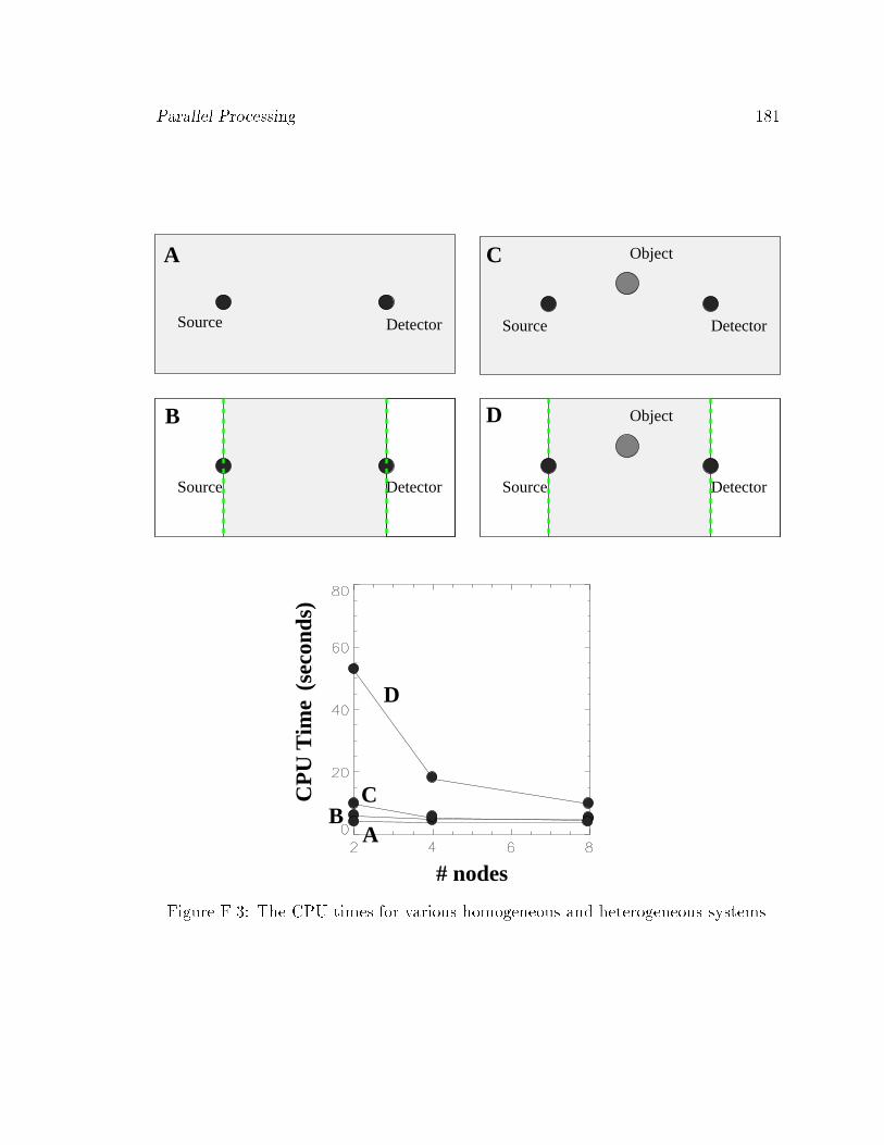
Parallel Processing 181
Source
ObjectD
C
Detector
A
(sec
onds
)C
PU
Tim
e
C
D
# nodes
DetectorSource
Object
Source Detector
Source Detector
B
BA
Figure F.3: The CPU times for various homogeneous and heterogeneous systems.
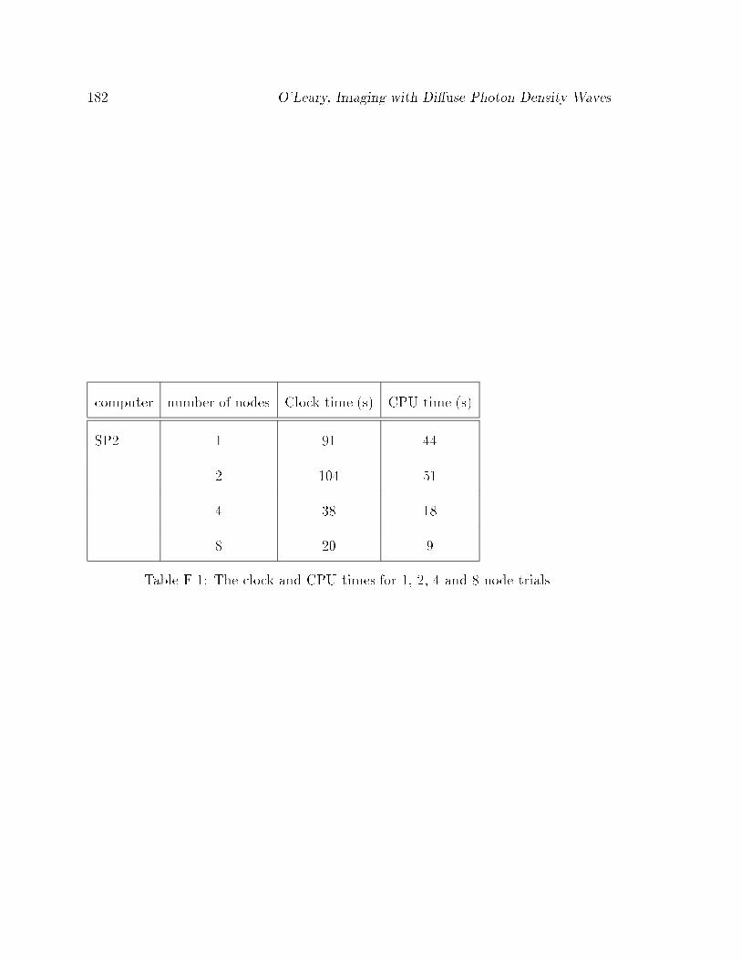
182 O'Leary, Imaging with Di�use Photon Density Waves
computer number of nodes Clock time (s) CPU time (s)
SP2 1 91 44
2 104 51
4 38 18
8 20 9
Table F.1: The clock and CPU times for 1, 2, 4 and 8 node trials.
Bibliography
[1] M. Cutler, , Surg. Gynecol. Obstet. 48, 721 (1929).
[2] S. Nioka, M. Miwa, S. Orel, M. Shnall, M. Haida, S. Zhao, and B. Chance,
Oxygen Transport to Tissue (Plenum Press, New York, 1994), pp. 171{179.
[3] M. Patterson, B. Chance, and B. Wilson, Time resolved re ectance and trans-
mittance for the non-invasive measurement of tissue optical properties, Applied
Optics 28(12), 2331 (1988).
[4] E. Gratton, W. Mantulin, M. J. van de Ven, J. Fishkin, M. Maris, and B. Chance,
Proceeding of the Third International Conference: Peace Through Mind/Brain
Science (Hamamatsu Photonics KK, Hamamatsu, Japan, 1990), p. 183.
[5] J. B. Fishkin and E. Gratton, Propagation of photon density waves in strongly
scattering media containing an absorbing semi-in�nite plane bounded by a
straight edge, J. Opt. Soc. of America A 10, 127 (1993).
[6] M. A. O'Leary, D. A. Boas, B. Chance, and A. G. Yodh, Refraction of di�use
photon density waves, Phys. Rev. Let. 69, 2658 (1992).
[7] D. A. Boas, M. A. O'Leary, B. Chance, and A. G. Yodh, Scattering and wave-
length transduction of di�use photon density waves, Phys. Rev. E 47, R2999
(1993).
[8] B. J. Tromberg, L. O. Svaasand, T. T. Tsay, and R. C. Haskell, Properties of
photon density waves in multiple scattering media, Applied Optics 32(4), 607
(1993).
183
184 O'Leary, Imaging with Di�use Photon Density Waves
[9] B. Chance, K. Kang, L. He, J. Weng, and E. Sevick, Highly sensitive object lo-
cation in tissue models with linear in-phase and anti-phase multi-element optical
arrays in one and two dimensions, Proc. Natl. Acad. Sci. 90, 3423 (1993).
[10] D. A. Boas, M. A. O'Leary, B. Chance, and A. G. Yodh, Scattering of di�use
photon density waves by spherical inhomogeneties within turbid media: analytic
solution and applications, Proc. Natl. Acad. Sci. USA 91, 4887 (1994).
[11] M. A. O'Leary, D. A. Boas, B. Chance, and A. G. Yodh, Reradiation and imaging
of di�use photon density waves using uorescent inhomogeneities, Journal of
Luminescence 60-61, 281 (1994).
[12] M. A. O'Leary, D. A. Boas, B. Li, X. D. Chance, and A. G. Yodh, Fluorescence
lifetime imaging in turbid media, Optics Letters 21, 158 (1996).
[13] S. Fantini, M. A. Franceschini, G. Gaida, E. Gratton, H. Jess, and W. W. Man-
tulin, Frequency-domain optical mammography: edge e�ect corrections, Med.
Phys. 23, 1 (1996).
[14] J. van Houten, D. Benaron, S. Spilman, and D. Stevenson, Imaging brain injury
using time-resolved near-infrared light scanning, Pediatric Research 39(3), 470
(1996).
[15] S. Fantini, M. Franceschini, S. A. Walker, J. S. Maier, and E. Gratton, Photon
path distributions in turbid media: applications for imaging in Optical Tomog-
raphy, Photon Migration and Spectroscopy of Tissue and Model Media; Theory,
Human Studies and Instrumentation (SPIE Optical Engineering Press, Belling-
ham, WA, 1995), Vol. 2389, pp. 340{349.
[16] J. C. Schotland, J. C. Haselgrove, and J. S. Leigh, Photon hitting density, Applied
Optics 32, 448 (1993).
[17] J. Chang, H. L. Graber, and R. L. Barbour, Image reconstruction of dense scat-
tering media from CW sources using constrained CGD and a matrix scaling
Bibliography 185
technique in Proceedings of Optical Tomography, Photon Migration, and Spec-
troscopy of Tissues and Model Media: Theory, Human Studies, and Instrumen-
tation (SPIE Optical Engineering Press, Bellingham, WA, 1995), pp. 682{691.
[18] M. A. O'Leary, D. A. Boas, B. Chance, and A. G. Yodh, Experimental images
of heterogeneous turbid media by frequency-domain di�using-photon tomography,
Optics Letters 20, 426 (1995).
[19] S. Arridge, P. van der Zee, M. Cope, and D. Delpy, Reconstruction method for in-
frared absorption imaging in Time Resolved Spectroscopy and Imaging of Tissues
(SPIE Optical Engineering Press, Bellingham, WA, 1991), Vol. 1431, p. 204.
[20] B. W. Pogue, M. S. Patterson, and T. J. Farrell, Forward and inverse calculations
for frequency domain di�use optical tomography in Optical Tomography,Photon
Migration and Spectroscopy of Tissue and Model Media; Theory, Human Studies
and Instrumentation (SPIE Optical Engineering Press, Bellingham, WA, 1995),
Vol. 2389, p. 328.
[21] C. L. Hutchinson, T. L. Troy, and E. M. Sevick-Muraca, Fluorescence lifetime
spectroscopy and imaging in random media in Optical Tomography,Photon Mi-
gration and Spectroscopy of Tissue and Model Media; Theory, Human Studies
and Instrumentation (SPIE Optical Engineering Press, Bellingham, WA, 1995),
Vol. 2389, p. 274.
[22] D. A. Boas, M. A. O'Leary, B. Chance, and A. G. Yodh, Detection and charac-
terization of optical inhomogeneities with di�use photon density waves: a signal
to noise analysis., J. Opt. Soc. A, special edition of Di�using Light Probes of
Turbid Media, accepted for publication (1996).
[23] C. L. Matson, N. Clark, L. McMackin, and J. S. Fender, Three-dimensional
tumor localization in thick tissue using measurements in a plane in Advances in
Optical Imaging and Photon Migration (Opt. Soc. Am., Washington D.C., 1996).
186 O'Leary, Imaging with Di�use Photon Density Waves
[24] J. S. Schotland, Inversion formulae for di�usion imaging in Optical Tomography,
Photon Migration and Spectroscopy of Tissue and Model Media; Theory, Human
Studies and Instrumentation (SPIE Optical Engineering Press, Bellingham,WA,
1995), Vol. 2389, pp. 304{310.
[25] M. Ishii, J. S. Leigh, and J. Schotland, Photon di�usion imaging in model and
biological systems in Optical Tomography, Photon Migration and Spectroscopy of
Tissue and Model Media; Theory, Human Studies and Instrumentation (SPIE
Optical Engineering Press, Bellingham, WA, 1995), Vol. 2389, p. 312.
[26] D. Pattanayuk, General Electric Consumer Research and Development Report
on Resolution of optical images formed by di�usive waves in highly scattering
media.
[27] A 3 mW, 780 nm source is modulated at 200 MHz. The turbid medium is 6.0 cm
thick with a reduced scattering coe�cient, �0s, of 10.0 cm�1 and �a = 0:05 cm�1.
An spherical object is embedded in the middle of the slab. Light is collected
and delivered to a photo-multiplier tube via an optical �ber with a diameter of
0.4 cm. For the simulations, the source and detector are scanned together along
the boundary or the source is held �xed close to the object and the detector
is scanned. Two di�erent objects are studied; an absorbing object with �0s;in =
10:0 cm�1 and �a;in = 0:15 cm�1 and a scattering object with �0s;in = 15:0 cm�1
and �a;in = 0:05 cm�1. For a positional uncertainty of 10 �m in either the source
or the detector, the fractional error in the amplitude is 2x10�3 and the phase
noise is 0:03�.
[28] M. A. O'Leary, D. A. Boas, B. Chance, and A. G. Yodh, Images of inhomogeneous
media using di�use photon density waves in Advances in Optical Imaging and
Photon Migration (Opt. Soc. Am., Washington D.C., 1994), Vol. 21, pp. 106{
115.
Bibliography 187
[29] D. A. Boas, L. E. Campbell, and A. G. Yodh, Scattering and imaging with
di�using temporal �eld correlation, Phys. Rev. Lett. 75, 1855 (1995).
[30] B. Beauvoit, S. Evans, T. Jenkins, E. Miller, and B. Chance, Correlation be-
tween the light-scattering and the mitochondrial content of normal-tissues and
transplantable rodent tumors, Analytical Biochemistry 226(1), 167 (1995).
[31] B. Beauvoit, T. Kitai, H. Liu, and B. Chance, Time-resolved spectroscopy of
mitochondria, cells, and rat tissues under normal and pathological conditions,
SPIE Optical Engineering Press 2326, 127 (1993).
[32] M. Kohl, M. Cope, M. Essenpreis, and D. Bocker, In uence of glucose-
concentration on light-scattering in tissue-simulating phantoms, Optics Letters
19(24), 2170 (1994).
[33] S. B. Bambot, J. R. Lakowitz, and G. Rao, Potential applications of lifetime-
based phase-modulation uorimetry in bioprocess and clinical monitoring, Trends
in Biotechnology 13(3), 106 (1993).
[34] J. B. Fishkin, O. Coquoz, E. R. Anderson, M. Brenner, and B. J. Tromberg,
Frequency-domain photon migration measurements of normal and malignant tis-
sue optical properties in a human subject, J. Opt. Soc. A, accepted (1996).
[35] The Intralipid used here can be obtained from The Hospital of the University of
Pennsylvania, Philadelphia, Pennsylvania.
[36] H. van Staveren, C. J. M. Moes, J. van Marle, S. A. Prahl, and J. C. van
Gemert, Light scattering in intralipid-10% in the wavelength range of 400-1100
nm, Applied Optics 30(31), (1991).
[37] E. Hecht, Optics (Addison-Wesley, Reading, MA, 1987), Chap. 4, 5, 6.
[38] J. Weng, M. Z. Zhang, K. Simons, and B. Chance, Measurement of biological
tissue metabolism using phase modulation spectroscopic technology in Time Re-
188 O'Leary, Imaging with Di�use Photon Density Waves
solved Spectroscopy and Imaging of Tissues (SPIE Optical Engineering Press,
Bellingham, WA, 1991), Vol. 1431, p. 161.
[39] As 780 nm light �elds with an optical frequency ! � 1016Hz impinge on a
photocathode, the emission of photoelectrons is proportional to the square of
the �eld. The square of the �eld has a part oscillating at 2! and a dc part. In
our case the detector speed is much slower than 1=2!, so oscillations average to
zero, and we only measure the dc part. For this reason we are able to ignore the
optical frequency in our calculation of the measured intensity.
[40] There are factors such as the quantum e�ciency of the photocathode, the actual
gain of the dynode chain, etc. which we do not attempt to measure. Instead
we either calibrate the device on a known model system or make relative mea-
surements. In addition, there are phase shifts induced as the modulated light
passes through an optical �ber, and as electric signals pass through capacitors
and lengths of cable.
[41] Photodiodes, Hamamatsu Photonics K.K., Solid State Division, Japan (1995).
[42] S. Yokoyama, A. Okamoto, A. Tsutomu, and S. Norihito, Examination to elim-
inate undesirable phase delay of an avalanche photodiode (APD) for intensity
modulated light, Rev. Sci. Instr. 66(11), 5331 (1995).
[43] The frequency drift of the phase locked Rhode & Schwatz generators drift is less
than we are capable of measuring. The upper limit on the phase locked generators
(measured with the SRS530) is 0.1 kHz/hour drift.
[44] Mini-Circuits, RF/IF Designer's Handbook, New York, 1992/93.
[45] A. G. Yodh and B. Chance, Spectroscopy and imaging with di�using light, Physics
Today 48(3), 34 (1995).
[46] Advances in Optical Imaging and Photon Migration (Opt. Soc. Am., Washington
D.C., 1994), Vol. 21.
Bibliography 189
[47] Medical Optical Tomography: Functional Imaging and Monitoring (SPIE Optical
Engineering Press, Bellingham, WA, 1993), Vol. Is11.
[48] A. C. Kak and M. Slaney, Principles of Computerized Tomographic Imaging
(IEEE Press, New York, 1988).
[49] This is not true at the source position. Thus we have assumed here that we will
not be reconstructing the region containing the source.
[50] M. S. Patterson and B. W. Pogue, E�ect of �nite volumes on noninvasive fre-
quency domain measurements of tissue properties in Advances in Optical Imaging
and Photon Migration (Opt. Soc. Am., Washington D.C., 1994), Vol. 21, p. 96.
[51] W. H. Press, S. A. Teukolsky, W. T. Vetterling, and B. P. Flannery, Numerical
Recipes in C: The Art of Scienti�c Computing (Cambridge University Press, New
York, 1988).
[52] G. E. Forsythe, M. A. Malcolm, and C. B. Moler, Computer Methods for Math-
ematical Computations (Prentice Hall, Englewood Cli�s, N.J., 1977), Chap. 9.
[53] C. P. Gonatas, personal communication.
[54] K. Tanube, , Numererical Mathematics 17, 203 (1971).
[55] M. Firbank, M. Hiraoka, and D. Delpy, A design for a stable and reproducible
phantom for use in near infra-red imaging and spectroscopy, Phys. Med. Biol.
38, 847 (1993).
[56] S. L. Jaques, M. R. Ostermeyer, L. Wang, and A. H. Hielscher, E�ects of sources,
boundaries and heterogeneities on photon migration in Advances in Optical Imag-
ing and Photon Migration (Opt. Soc. Am., Washington D.C., 1994), Vol. 21, p.
83.
190 O'Leary, Imaging with Di�use Photon Density Waves
[57] R. L. Barbour, H. L. Graber, J. W. Chang, S. L. S. Barbour, P. C. Koo, and R.
Aronson, MRI-guided optical tomography{prospects and computation for a new
imaging method, IEEE Computational Science & Engineering 2(4), 63 (1995).
[58] M. Schweiger and S. R. Arridge, Near-infrared imaging: photon measurement
density functions in Optical Tomography, Photon Migration and Spectroscopy of
Tissue and Model Media; Theory, Human Studies and Instrumentation (SPIE
Optical Engineering Press, Bellingham, WA, 1995), Vol. 2389, pp. 366{388.
[59] S. Arridge, M. Cope, and D. T. Delpy, The theoretical basis for the determination
of optical pathlengths in tissue: a temporal and frequency domain analysis, Phys.
Med. Biol. 37(7), 1531 (1992).
[60] R. C. Haskell, L. O. Svaasand, T. Tsay, T. Feng, M. S. McAdams, and B. J.
Tromberg, Boundary conditions for the di�usion equation in radiative transfer,
J. Opt. Soc. Amer. A 11, 2727 (1994).
[61] S. Glasstone and M. C. Edlund, in The Elements of Nuclear Reactor Theory (D.
van Nostrand Co., New York, 1952), Chap. 5 & 14.
[62] K. M. Case and P. F. Zweifel, in Linear Transport Theory (Addison-Wesley, MA,
1967), Chap. 8.
[63] R. Aronson, Boundary conditions for di�usion of light, J. Opt. Soc. Amer. A 12,
2532 (1995).
[64] K. M. Case and P. F. Zweifel, Linear Transport Theory (Addison-Wesley, MA,
1967).
[65] J. D. Jackson, Classical Electrodynamics (John Wiley & Sons, New York, NY,
1975).
[66] J. Virmont and G. Ledanois, Near-infrared medical imaging direct and inverse
problem in Advances in Optical Imaging and Photon Migration, Technical Digest
(Opt. Soc. Am., Washington D.C., 1996).
Bibliography 191
[67] E. M. Sevick-Muraca and C. L. Burch, Origin of phosphorescence signals reemit-
ted from tissues, Optics Letters 19(23), 1928 (1994).
[68] M. S. Patterson and B. W. Pogue, Mathematical-model for time-resolved and
frequency-domain uorescence spectroscopy in biological tissue, Applied Optics
33(10), 1963 (1994).
[69] A. Kn�uttel, J. M. Schmitt, R. Barnes, and J. R. Knutson, Acousto-optic scanning
and interfering photon density waves for precise localization of an absorbing (or
uorescent) body in a turbid medium, Rev. Sci. Instrum. 64, 638 (1993).
[70] X. D. Li, B. Beauvoit, R. White, S. Nioka, B. Chance, and A. G. Yodh, Tu-
mor localization using uorescence of indocyanine green in Optical Tomography,
Photon Migration and Spectroscopy of tissue and Model Media; Theory, Human
Studies and Instrumentation (SPIE Optical Engineering Press, Bellingham,WA,
1995), Vol. 2398, p. 789.
[71] J. Wu, Y. Wang, L. Perelman, I. Itzkan, R. R. Dasari, and M. S. Feld, Time-
resolved multichannel imaging of uorescent objects embedded in turbid media,
Optics Letters 20, 489 (1995).
[72] W. L. Rumsey, J. M. Vanderkooi, and D. F. Wilson, Imaging of phosphorescence:
a novel method for measuring oxygen distribution in perfused tissue, Science 241,
1649 (1988).
[73] H. Szmacinski and J. R. Lakowicz, Optical measurements of pH using uores-
cence lifetimes and phase-modulation uorometry, Analytical Chemistry 65, 1668
(1993).
[74] J. R. Lakowicz, H. Szmacinski, K. Nowaczyk, and M. L. Johnson, Fluorescence
lifetime imaging of calcium using Quin-2, Cell Calcium 13, 131 (1992).
[75] J. Folkman, Introduction: Angiogenesis and cancer, seminars in Cancer Biology
3, 65 (1992).
192 O'Leary, Imaging with Di�use Photon Density Waves
[76] P. W. Vaupel, S. Frinak, and H. I. Bicher, Heterogeneous oxygen partial pressure
and pH distribution in C3H mouse mammary adenocarcinoma, Cancer Research
41, 2008 (1981).
[77] C. L. Hutchinson, J. R. Lakowicz, and E. Sevick-Muraca, Fluorescence lifetime-
based sensing in tissues: a computational study, Biophysical Journal 68, 1574
(1995).
[78] J. Wu, M. S. Feld, and R. P. Rave, Analytical model for extracting intrinsic
uorescence in turbid media, Applied Optics 32(19), 3585 (1993).
[79] X. D. Li, M. A. O'Leary, D. A. Boas, B. Chance, and A. G. Yodh, Fluorescent
di�use photon{density waves in homogeneous and heterogeneous turbid media -
analytic solutions and applications, Applied Optics 35(19), 3746 (1996).
[80] Cardio-Green is a water soluble, tricarbocyanine dye. We obtained the dye from
Hynson, Wescott Dunning, Inc., Baltimore, Md. 21201, USA.
[81] S. Zhau, M. A. O'Leary, S. Nioka, and B. Chance, Breast tumor detection us-
ing continuous wave light sources in Optical Tomography, Photon Migration and
Spectroscopy of tissue and Model Media; Theory, Human Studies and Instrumen-
tation (SPIE Optical Engineering Press, Bellingham, WA, 1995), Vol. 2398, pp.
809{817.
[82] Clinical breast imaging data are expected to be published soon by S. B. Colak,
Philips Research Labs, Netherlands.
[83] B. J. Tromberg, S. Madsen, C. Chapman, L. O. Svaasand, and R. C. Haskell,
Frequency-Domin photon migration in turbid media in Advances in Optical Imag-
ing and Photon Migration (Opt. Soc. Am., Washington D.C., 1994), Vol. 21.


![Elizabeth O'Leary - Macquarie Bank[1]](https://cdn.vdocuments.mx/doc/165x107/546823ccb4af9f3f3f8b5b46/elizabeth-oleary-macquarie-bank1.jpg)