MATLAB ® - The Language of Technical Computing
http://www.mathworks.com
What is MATLAB good for?
-Matrix calculations (MatLab= “Matrix”Lab)
-Manipulating and plotting data…especially large data sets.
-Scientific computing.
-Dynamic system modeling and control system design.
-Much, much more…

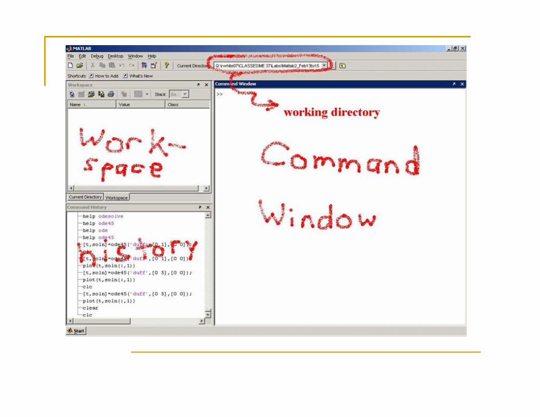
Start Matlab… under “Engineering and Science Applications” in the
START menu.
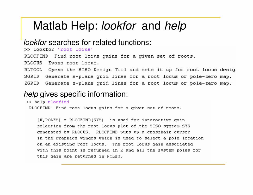
Matlab Help: lookfor and help
lookfor searches for related functions:
help gives specific information:
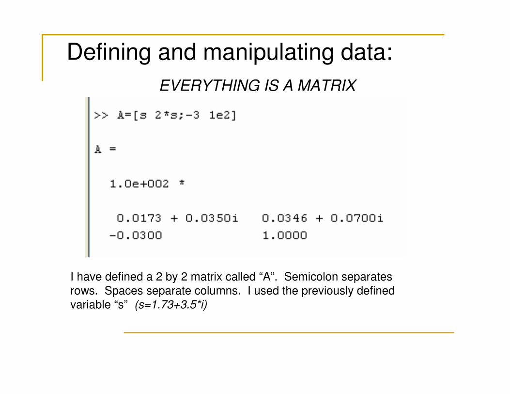
Defining and manipulating data:
EVERYTHING IS A MATRIX
I have defined a 2 by 2 matrix called “A”. Semicolon separates
rows. Spaces separate columns. I used the previously defined variable “s” (s=1.73+3.5*i)
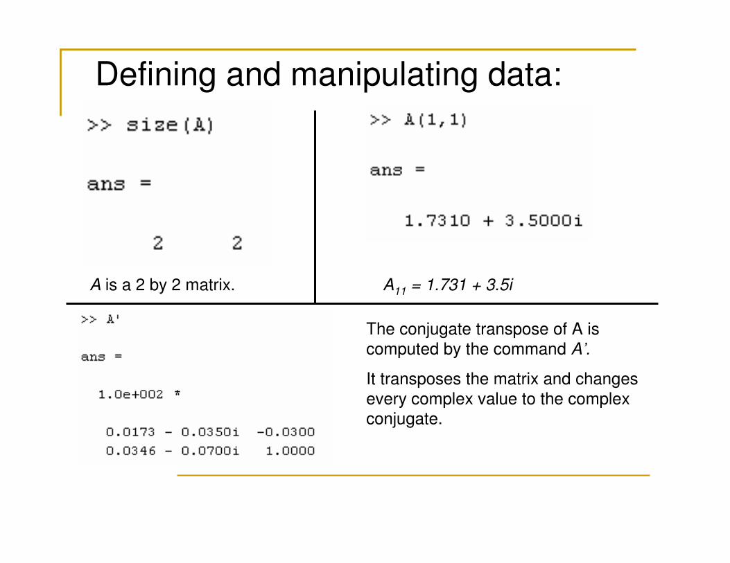
Defining and manipulating data:
A is a 2 by 2 matrix. A11 = 1.731 + 3.5i
The conjugate transpose of A is
computed by the command A’.
It transposes the matrix and changes
every complex value to the complex
conjugate.
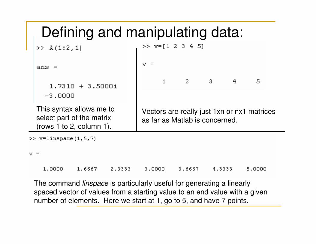
Defining and manipulating data:
This syntax allows me to
select part of the matrix
(rows 1 to 2, column 1).
Vectors are really just 1xn or nx1 matrices
as far as Matlab is concerned.
The command linspace is particularly useful for generating a linearly
spaced vector of values from a starting value to an end value with a given
number of elements. Here we start at 1, go to 5, and have 7 points.

Defining and manipulating data:
Strings are defined using single quotes:
There are a bunch of string manipulating
functions. Type help strfun
To refer to an entire column or row
of a matrix, you can just use the
colon operator with no numbers
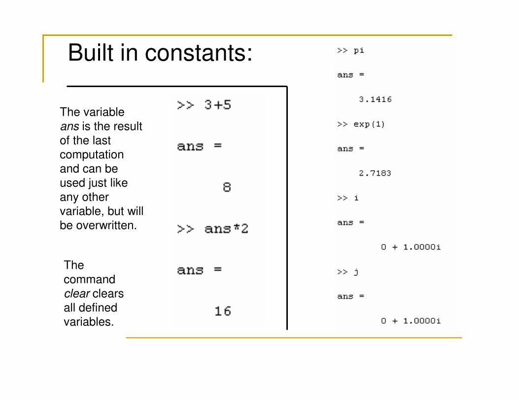
Built in constants:
The variable
ans is the result
of the last
computation and can be
used just like
any other
variable, but will be overwritten.
The
command
clear clears all defined
variables.
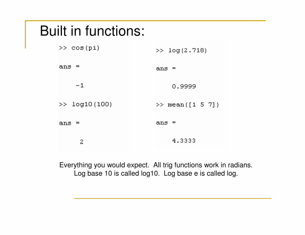
Built in functions:
Everything you would expect. All trig functions work in radians.
Log base 10 is called log10. Log base e is called log.
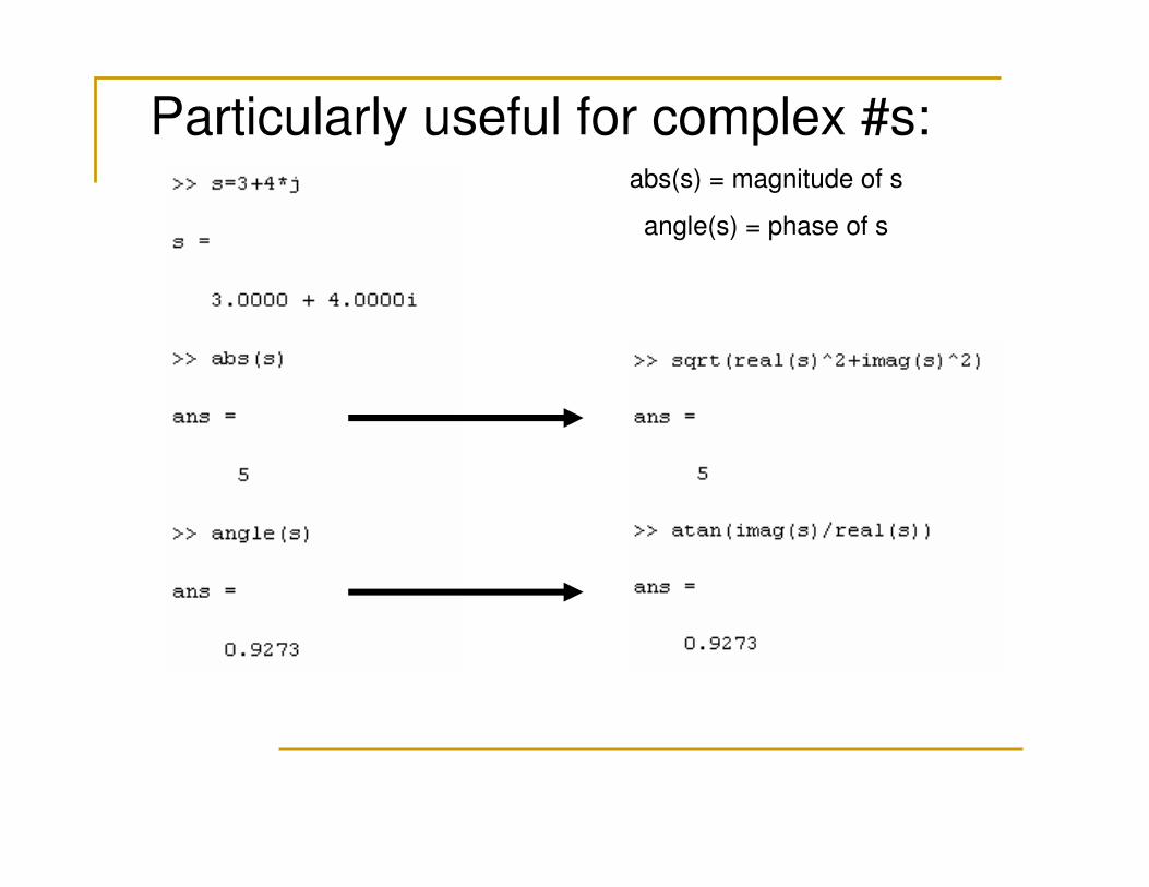
Particularly useful for complex #s:abs(s) = magnitude of s
angle(s) = phase of s
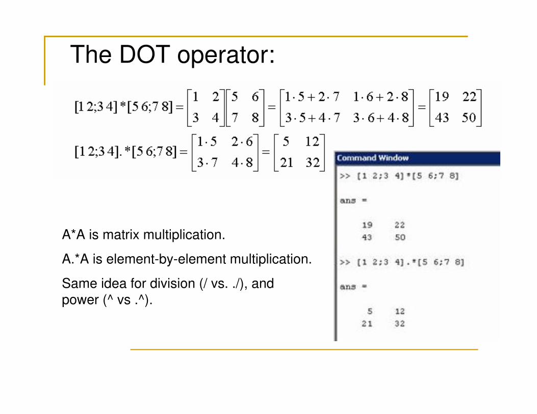
The DOT operator:
A*A is matrix multiplication.
A.*A is element-by-element multiplication.
Same idea for division (/ vs. ./), and power (^ vs .^).
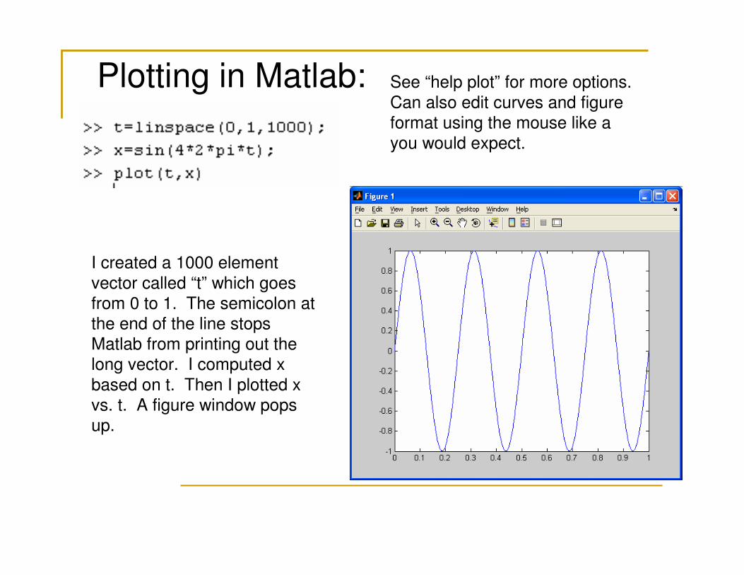
Plotting in Matlab:
I created a 1000 element
vector called “t” which goes
from 0 to 1. The semicolon at the end of the line stops
Matlab from printing out the
long vector. I computed x
based on t. Then I plotted x
vs. t. A figure window pops
up.
See “help plot” for more options.
Can also edit curves and figure
format using the mouse like a
you would expect.
Plotting in Matlab:
To open a new figure windows, type:
>> figure
To make figure 2 current, type:
>> figure(2)
Matlab will plot on the current figure. If there is already a plot there, it
will be overwritten, unless you first tell Matlab to hold the plot:
>> hold on
To turn off the hold,
>> hold off
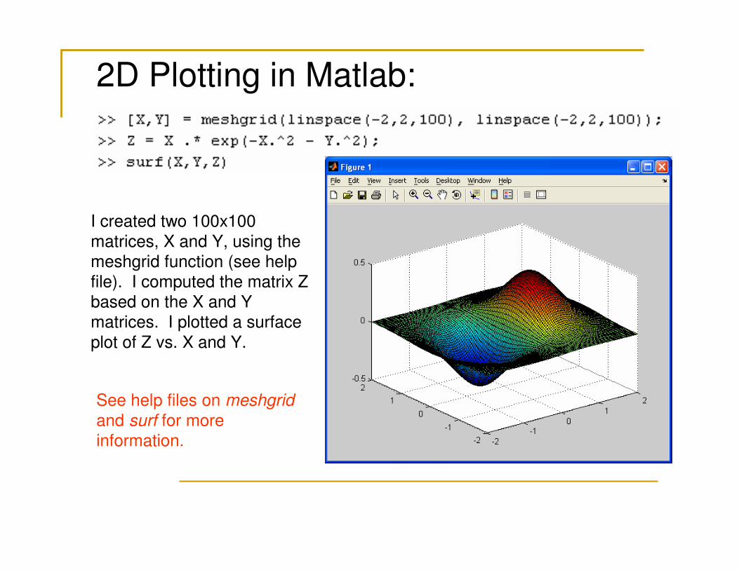
2D Plotting in Matlab:
I created two 100x100
matrices, X and Y, using the
meshgrid function (see help
file). I computed the matrix Z based on the X and Y
matrices. I plotted a surface
plot of Z vs. X and Y.
See help files on meshgrid
and surf for more information.
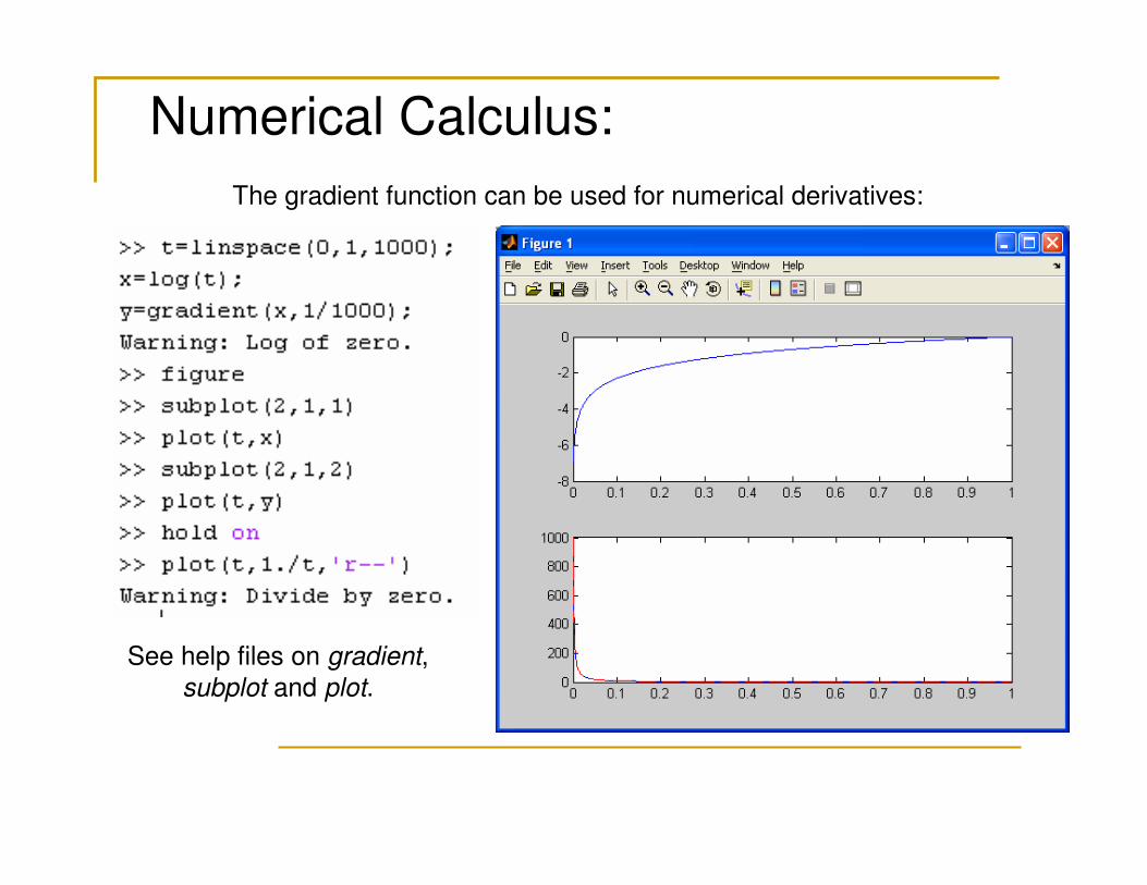
Numerical Calculus:
The gradient function can be used for numerical derivatives:
See help files on gradient,
subplot and plot.
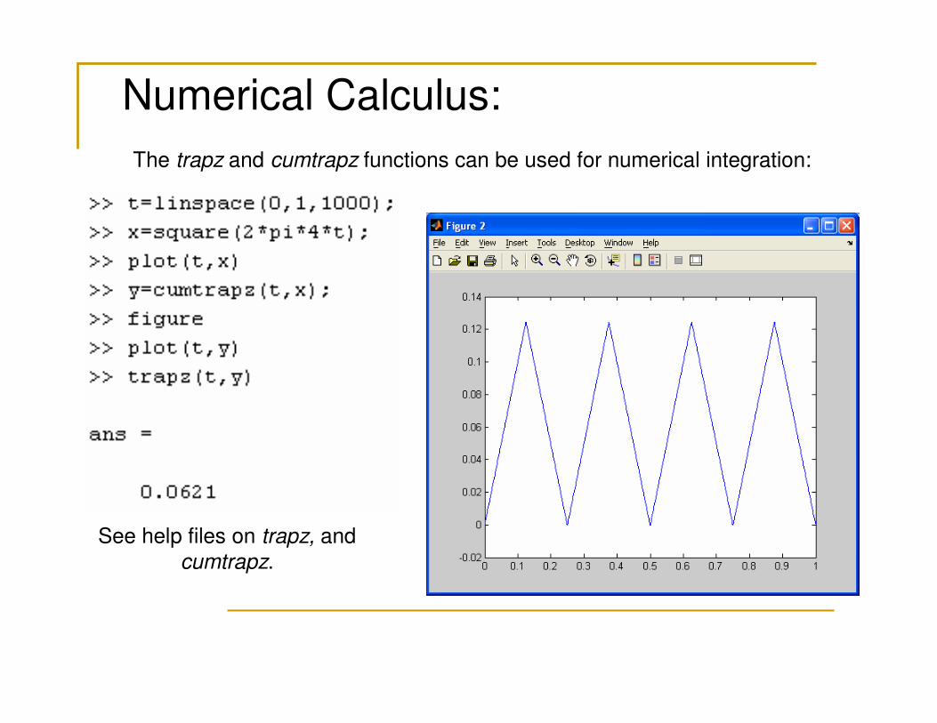
Numerical Calculus:
The trapz and cumtrapz functions can be used for numerical integration:
See help files on trapz, and
cumtrapz.
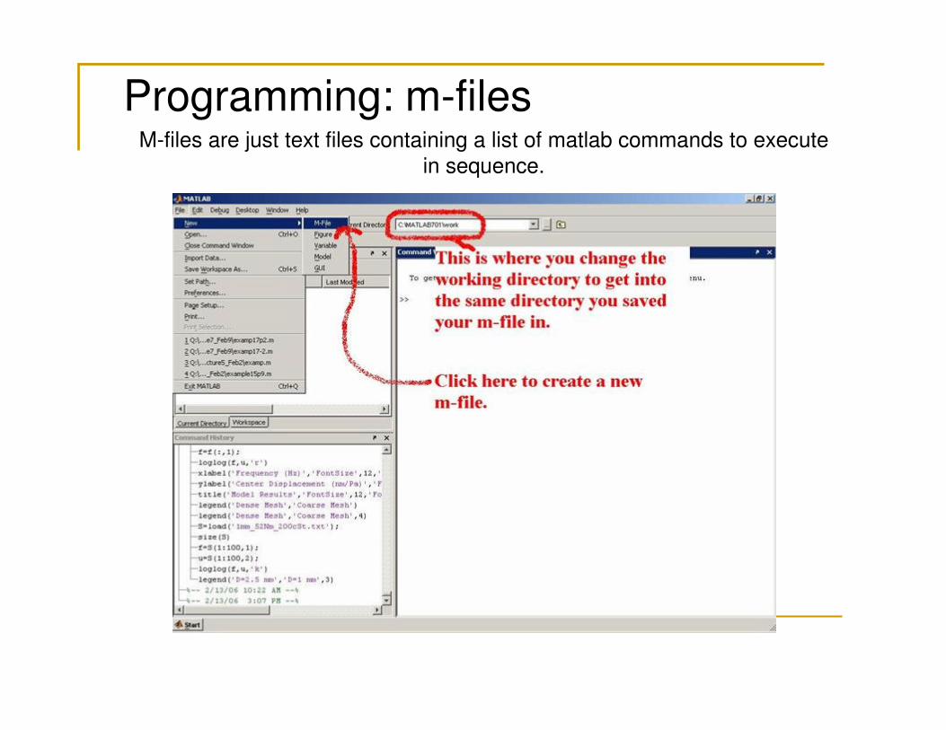
Programming: m-filesM-files are just text files containing a list of matlab commands to execute
in sequence.

Programming: m-filesHere is an m-file that computes the roots of a quadratic equation.
Note syntax for if statement. Note that any line starting with % is a comment.
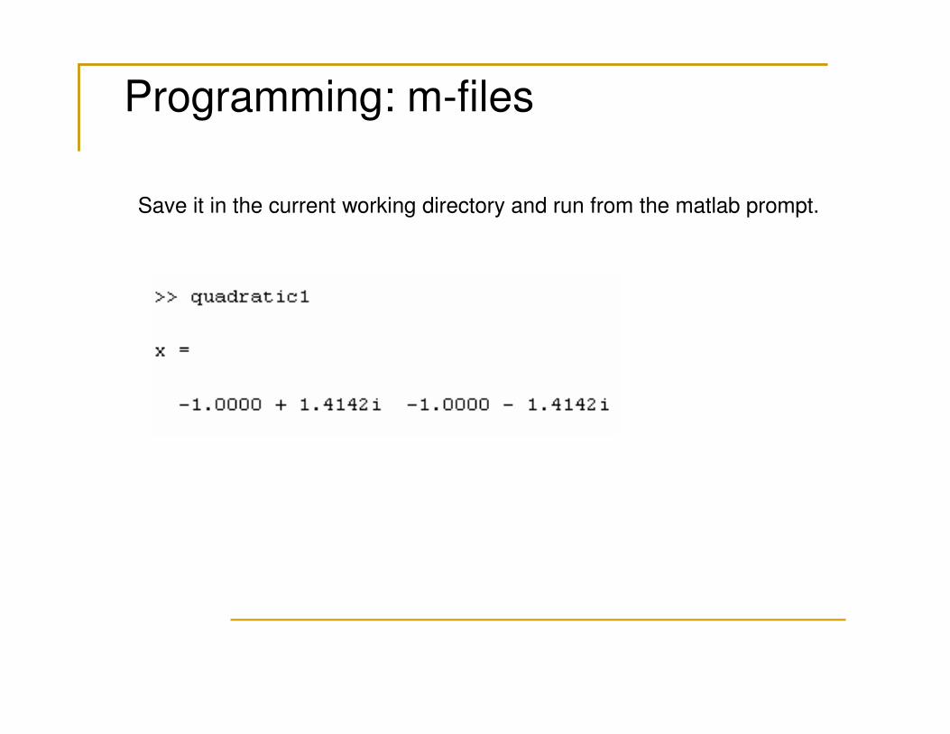
Programming: m-files
Save it in the current working directory and run from the matlab prompt.
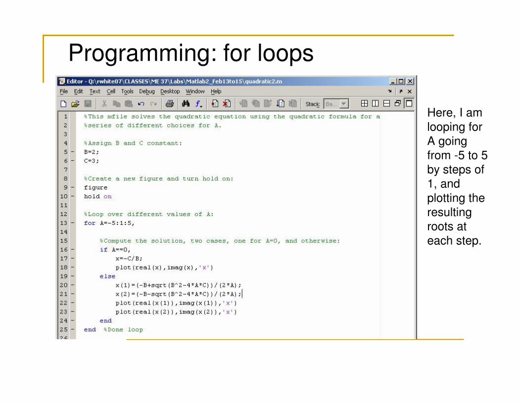
Programming: for loops
Here, I am
looping for
A going
from -5 to 5 by steps of
1, and
plotting the
resulting roots at
each step.
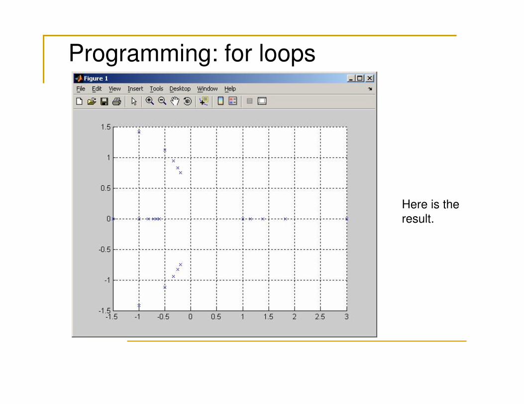
Programming: for loops
Here is the
result.
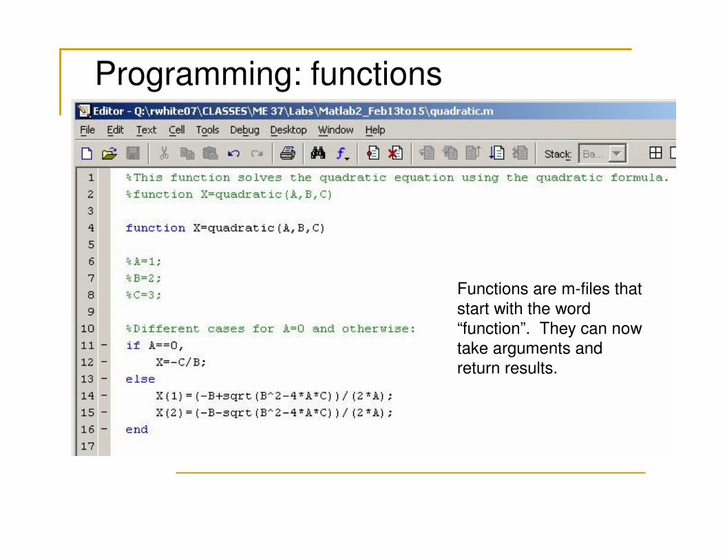
Programming: functions
Functions are m-files that
start with the word
“function”. They can now
take arguments and return results.
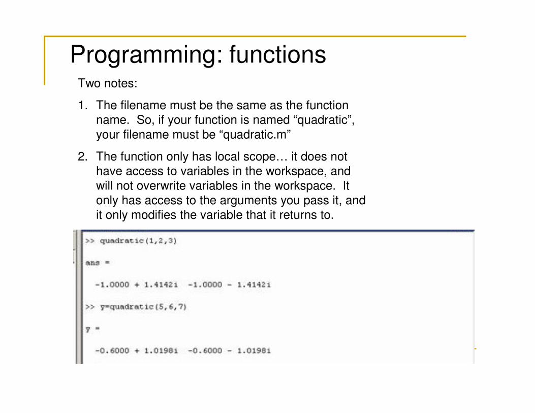
Programming: functionsTwo notes:
1. The filename must be the same as the function name. So, if your function is named “quadratic”,
your filename must be “quadratic.m”
2. The function only has local scope… it does not have access to variables in the workspace, and
will not overwrite variables in the workspace. It
only has access to the arguments you pass it, and
it only modifies the variable that it returns to.
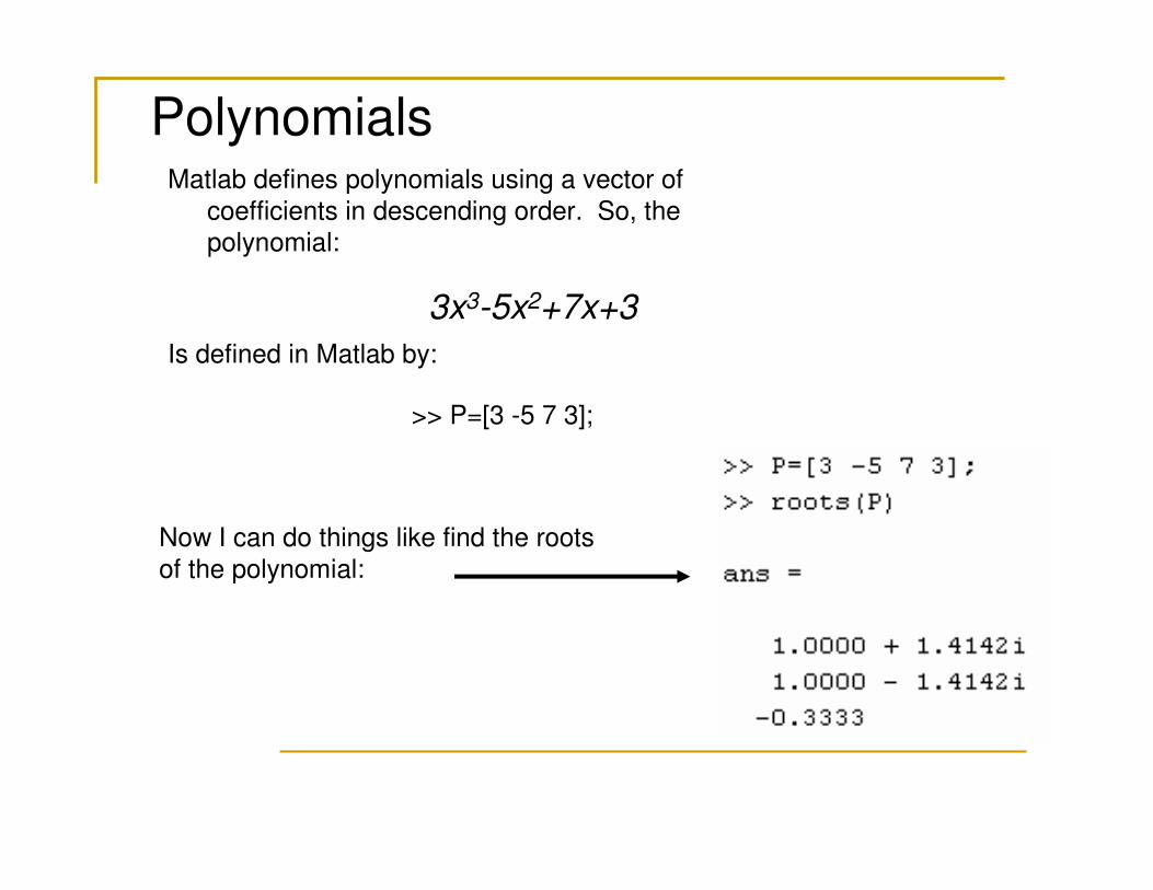
PolynomialsMatlab defines polynomials using a vector of
coefficients in descending order. So, the
polynomial:
3x3-5x2+7x+3
Is defined in Matlab by:
>> P=[3 -5 7 3];
Now I can do things like find the roots
of the polynomial:
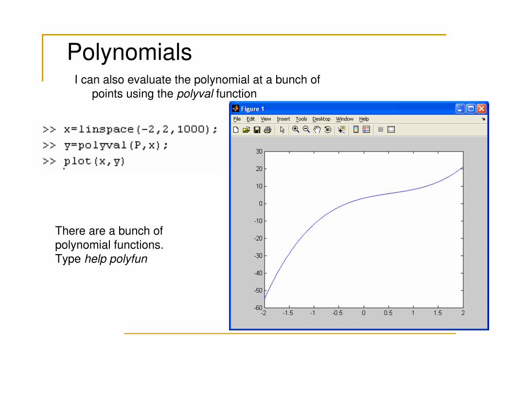
PolynomialsI can also evaluate the polynomial at a bunch of
points using the polyval function
There are a bunch of
polynomial functions. Type help polyfun
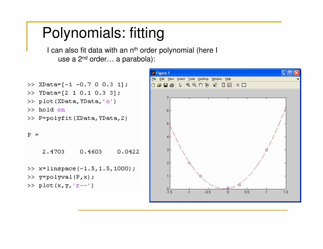
Polynomials: fittingI can also fit data with an nth order polynomial (here I
use a 2nd order… a parabola):
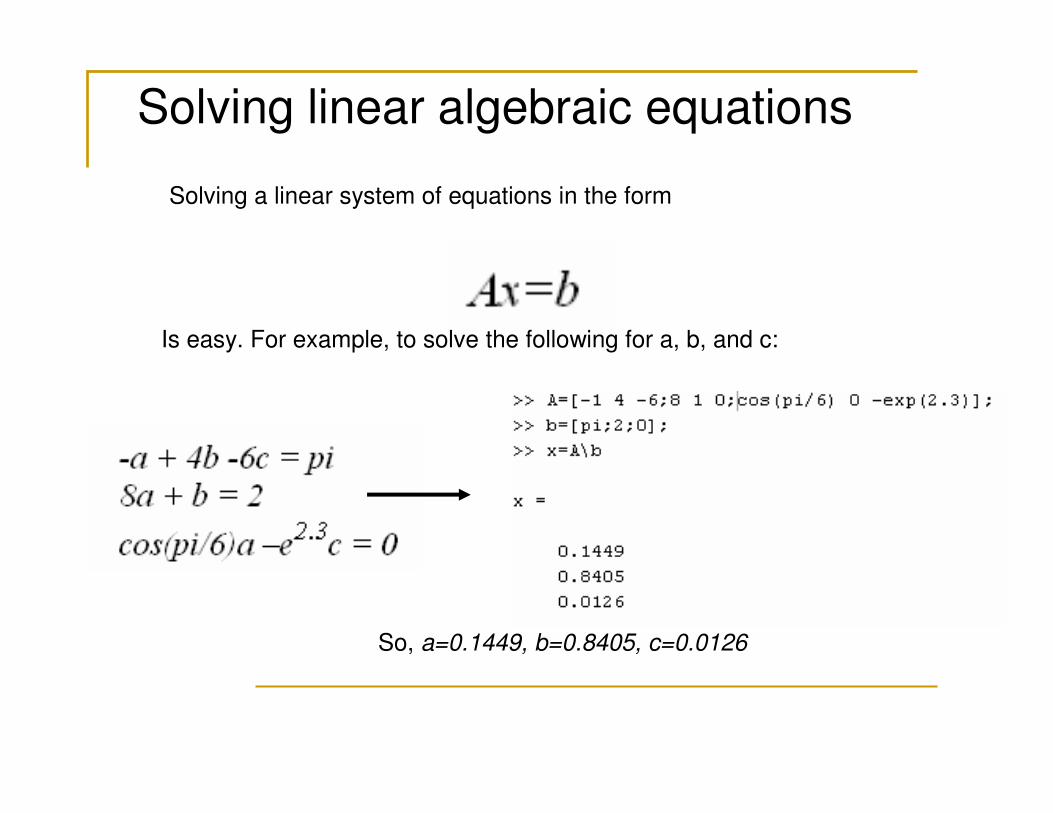
Solving linear algebraic equations
Solving a linear system of equations in the form
Is easy. For example, to solve the following for a, b, and c:
So, a=0.1449, b=0.8405, c=0.0126
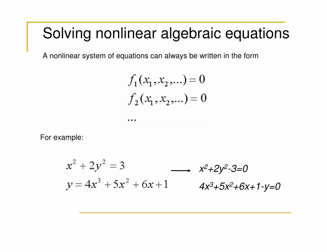
Solving nonlinear algebraic equations
A nonlinear system of equations can always be written in the form
For example:
x2+2y2-3=0
4x3+5x2+6x+1-y=0
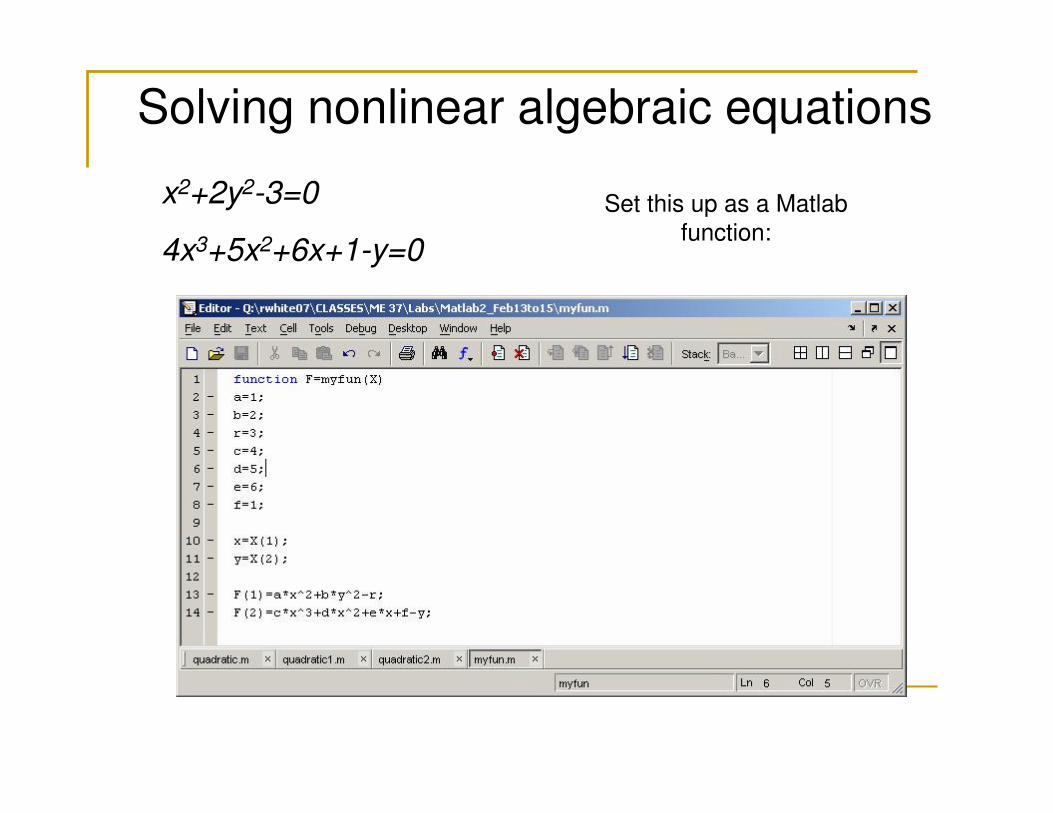
Solving nonlinear algebraic equations
x2+2y2-3=0
4x3+5x2+6x+1-y=0
Set this up as a Matlab
function:
Solving nonlinear algebraic equations
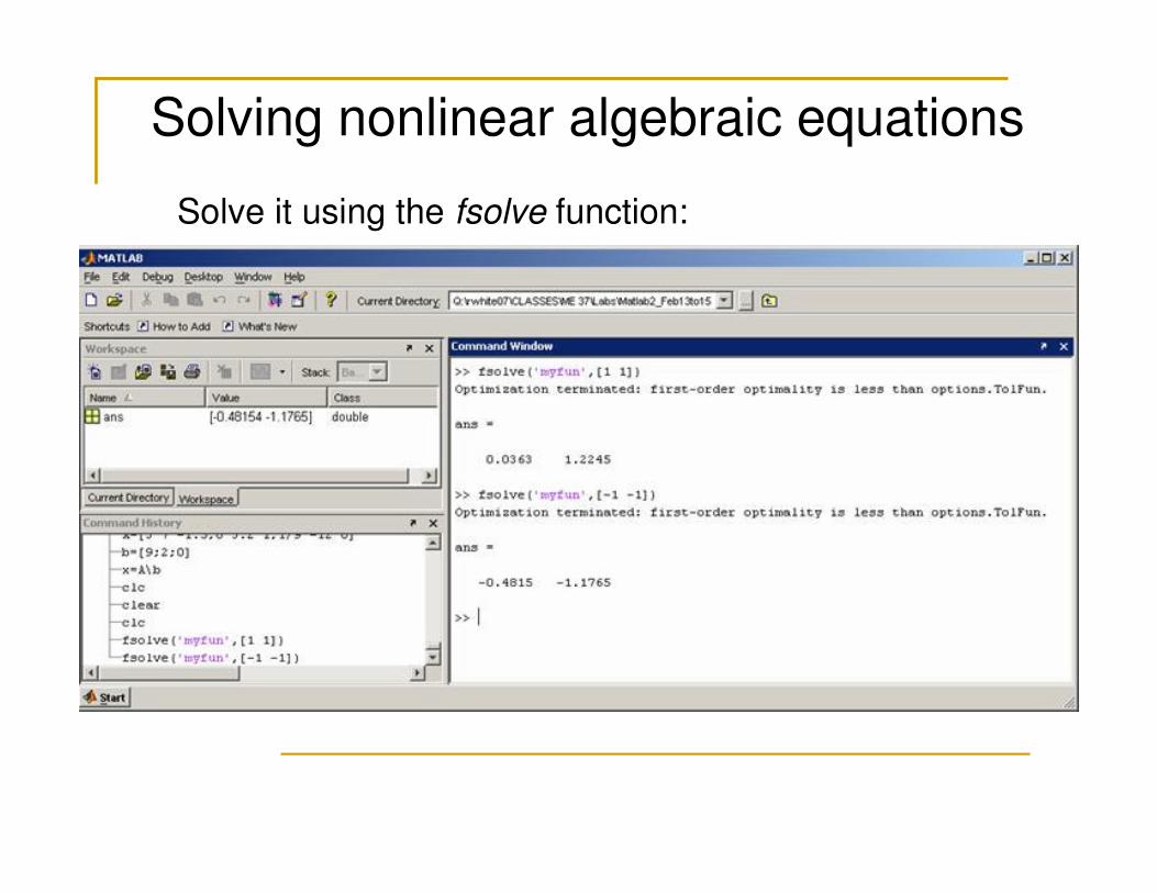
Solve it using the fsolve function:
Solving nonlinear algebraic equations
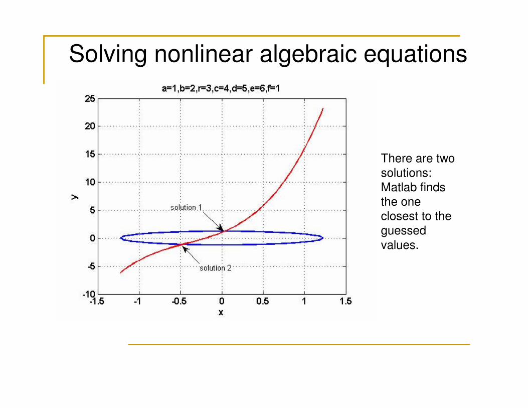
There are two
solutions:
Matlab finds
the one closest to the
guessed
values.
Solving ordinary differential equations
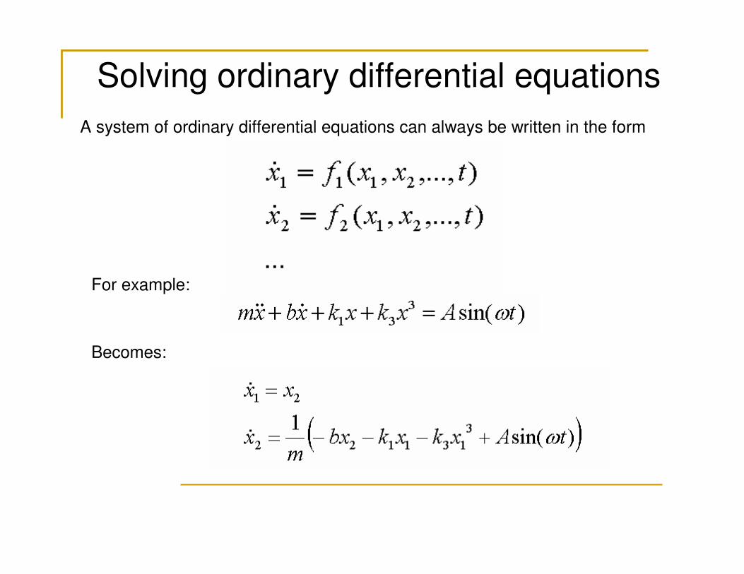
A system of ordinary differential equations can always be written in the form
For example:
Becomes:
Solving ordinary differential equations
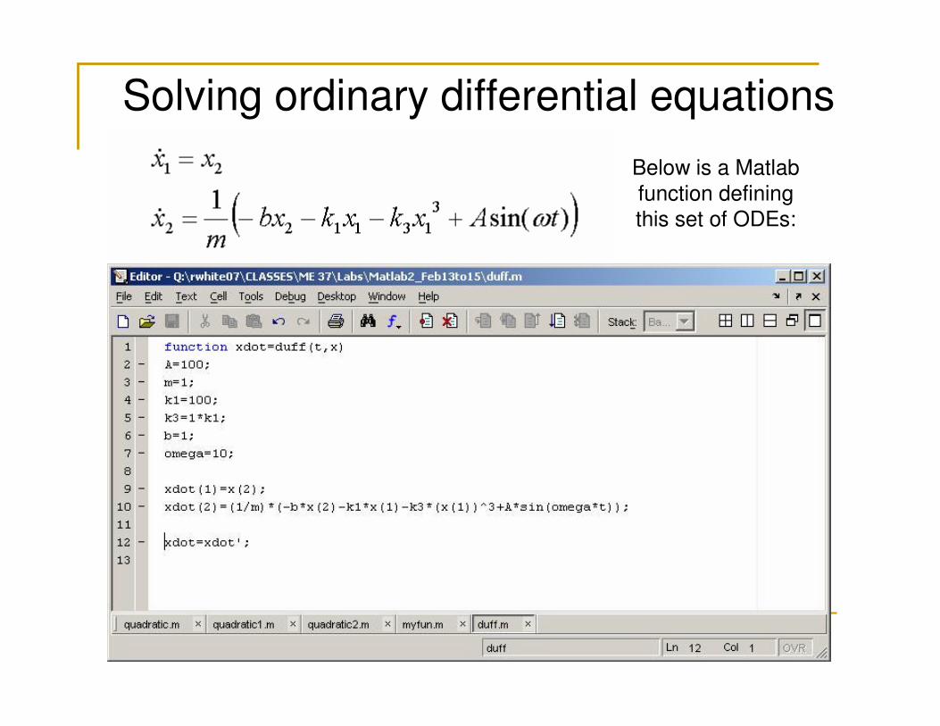
Below is a Matlab
function defining
this set of ODEs:
Solving ordinary differential equations
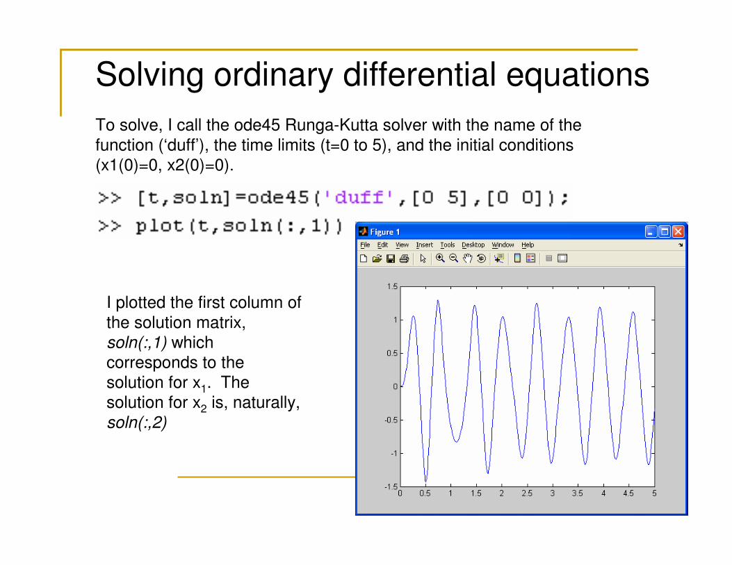
To solve, I call the ode45 Runga-Kutta solver with the name of the
function (‘duff’), the time limits (t=0 to 5), and the initial conditions
(x1(0)=0, x2(0)=0).
I plotted the first column of
the solution matrix,
soln(:,1) which
corresponds to the solution for x1. The
solution for x2 is, naturally,
soln(:,2)


