Logistic Regression:Online, Lazy, Kernelized, Sequential, etc.
Harsha Veeramachaneni
Thomson Reuter Research and Development
April 1, 2010
Harsha Veeramachaneni (TR R&D) Logistic Regression April 1, 2010 1 / 56
1 Logistic Regression (Plain and Simple)Introduction to logistic regression
2 Learning AlgorithmLog-LikelihoodGradient DescentLazy Updates
3 Kernelization
4 Sequence Tagging
Harsha Veeramachaneni (TR R&D) Logistic Regression April 1, 2010 2 / 56
1 Logistic Regression (Plain and Simple)Introduction to logistic regression
2 Learning AlgorithmLog-LikelihoodGradient DescentLazy Updates
3 Kernelization
4 Sequence Tagging
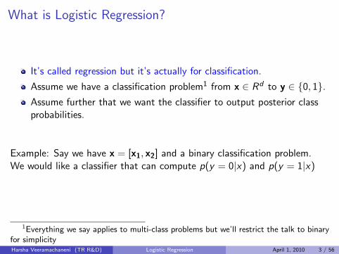
What is Logistic Regression?
It’s called regression but it’s actually for classification.
Assume we have a classification problem1 from x ∈ Rd to y ∈ {0, 1}.Assume further that we want the classifier to output posterior classprobabilities.
Example: Say we have x = [x1, x2] and a binary classification problem.We would like a classifier that can compute p(y = 0|x) and p(y = 1|x)
1Everything we say applies to multi-class problems but we’ll restrict the talk to binaryfor simplicityHarsha Veeramachaneni (TR R&D) Logistic Regression April 1, 2010 3 / 56
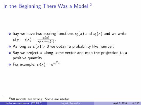
In the Beginning There Was a Model 2
Say we have two scoring functions s0(x) and s1(x) and we write
p(y = i |x) = si (x)s0(x)+s1(x) .
As long as si (x) > 0 we obtain a probability like number.
Say we project x along some vector and map the projection to apositive quantity.
For example, si (x) = ewTi x
2All models are wrong. Some are useful.Harsha Veeramachaneni (TR R&D) Logistic Regression April 1, 2010 4 / 56
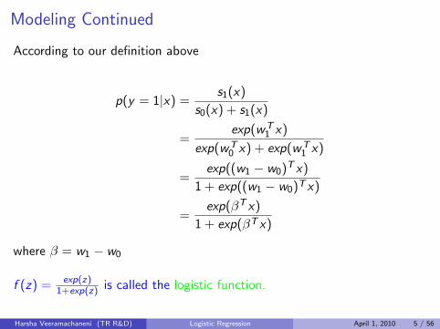
Modeling Continued
According to our definition above
p(y = 1|x) =s1(x)
s0(x) + s1(x)
=exp(wT
1 x)
exp(wT0 x) + exp(wT
1 x)
=exp((w1 − w0)T x)
1 + exp((w1 − w0)T x)
=exp(βT x)
1 + exp(βT x)
where β = w1 − w0
f (z) = exp(z)1+exp(z) is called the logistic function.
Harsha Veeramachaneni (TR R&D) Logistic Regression April 1, 2010 5 / 56
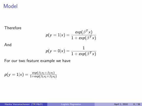
Model
Therefore
p(y = 1|x) =exp(βT x)
1 + exp(βT x)
And
p(y = 0|x) =1
1 + exp(βT x)
For our two feature example we have
p(y = 1|x) = exp(β1x1+β2x2)1+exp(β1x1+β2x2)
Harsha Veeramachaneni (TR R&D) Logistic Regression April 1, 2010 6 / 56
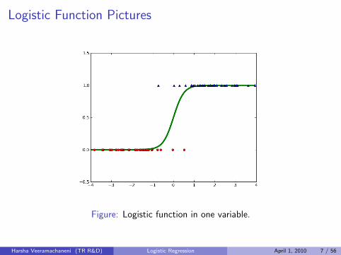
Logistic Function Pictures
Figure: Logistic function in one variable.
Harsha Veeramachaneni (TR R&D) Logistic Regression April 1, 2010 7 / 56
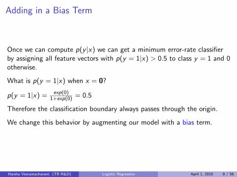
Adding in a Bias Term
Once we can compute p(y |x) we can get a minimum error-rate classifierby assigning all feature vectors with p(y = 1|x) > 0.5 to class y = 1 and 0otherwise.
What is p(y = 1|x) when x = 0?
p(y = 1|x) = exp(0)1+exp(0) = 0.5
Therefore the classification boundary always passes through the origin.
We change this behavior by augmenting our model with a bias term.
Harsha Veeramachaneni (TR R&D) Logistic Regression April 1, 2010 8 / 56
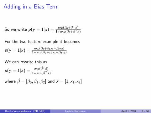
Adding in a Bias Term
So we write p(y = 1|x) = exp(β0+βT x)1+exp(β0+βT x)
For the two feature example it becomes
p(y = 1|x) = exp(β0+β1x1+β2x2)1+exp(β0+β1x1+β2x2)
We can rewrite this as
p(y = 1|x) = exp(β́T x́)
1+exp(β́T x́)
where β́ = [β0, β1, β2] and x́ = [1, x1, x2]
Harsha Veeramachaneni (TR R&D) Logistic Regression April 1, 2010 9 / 56
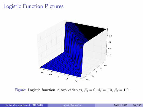
Logistic Function Pictures
Figure: Logistic function in two variables, β0 = 0, β1 = 1.0, β2 = 1.0
Harsha Veeramachaneni (TR R&D) Logistic Regression April 1, 2010 10 / 56
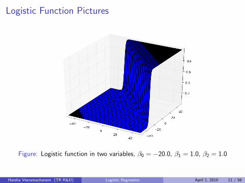
Logistic Function Pictures
Figure: Logistic function in two variables, β0 = −20.0, β1 = 1.0, β2 = 1.0
Harsha Veeramachaneni (TR R&D) Logistic Regression April 1, 2010 11 / 56
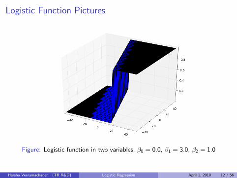
Logistic Function Pictures
Figure: Logistic function in two variables, β0 = 0.0, β1 = 3.0, β2 = 1.0
Harsha Veeramachaneni (TR R&D) Logistic Regression April 1, 2010 12 / 56
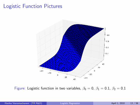
Logistic Function Pictures
Figure: Logistic function in two variables, β0 = 0, β1 = 0.1, β2 = 0.1
Harsha Veeramachaneni (TR R&D) Logistic Regression April 1, 2010 13 / 56
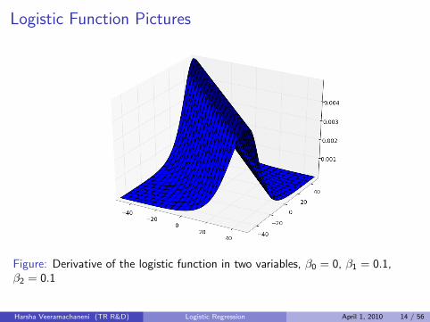
Logistic Function Pictures
Figure: Derivative of the logistic function in two variables, β0 = 0, β1 = 0.1,β2 = 0.1
Harsha Veeramachaneni (TR R&D) Logistic Regression April 1, 2010 14 / 56
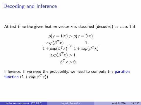
Decoding and Inference
At test time the given feature vector x is classified (decoded) as class 1 if
p(y = 1|x) > p(y = 0|x)
exp(βT x)
1 + exp(βT x)>
1
1 + exp(βT x)
exp(βT x) > 1
βT x > 0
Inference: If we need the probability, we need to compute the partitionfunction (1 + exp(βT x))
Harsha Veeramachaneni (TR R&D) Logistic Regression April 1, 2010 15 / 56
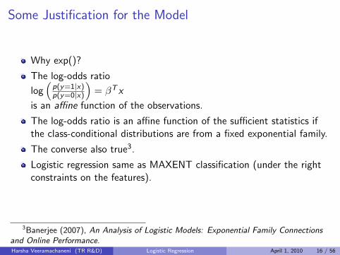
Some Justification for the Model
Why exp()?
The log-odds ratio
log(
p(y=1|x)p(y=0|x)
)= βT x
is an affine function of the observations.
The log-odds ratio is an affine function of the sufficient statistics ifthe class-conditional distributions are from a fixed exponential family.
The converse also true3.
Logistic regression same as MAXENT classification (under the rightconstraints on the features).
3Banerjee (2007), An Analysis of Logistic Models: Exponential Family Connectionsand Online Performance.Harsha Veeramachaneni (TR R&D) Logistic Regression April 1, 2010 16 / 56
1 Logistic Regression (Plain and Simple)Introduction to logistic regression
2 Learning AlgorithmLog-LikelihoodGradient DescentLazy Updates
3 Kernelization
4 Sequence Tagging
Learning
Suppose we are given a labeled data set
D = {(x1, y1), (x2, y2), . . . , (xN , yN)}
From this data we wish to learn the logistic regression parameter (weight)vector β.
Harsha Veeramachaneni (TR R&D) Logistic Regression April 1, 2010 17 / 56
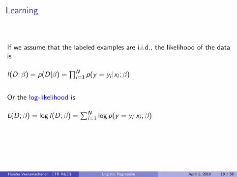
Learning
If we assume that the labeled examples are i.i.d., the likelihood of the datais
l(D;β) = p(D|β) =∏N
i=1 p(y = yi |xi ;β)
Or the log-likelihood is
L(D;β) = log l(D;β) =∑N
i=1 log p(y = yi |xi ;β)
Harsha Veeramachaneni (TR R&D) Logistic Regression April 1, 2010 18 / 56
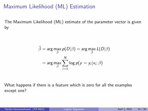
Maximum Likelihood (ML) Estimation
The Maximum Likelihood (ML) estimate of the parameter vector is givenby
β̂ = arg maxβ
p(D|β) = arg maxβ
L(D|β)
= arg maxβ
N∑i=1
log p(y = yi |xi ;β)
What happens if there is a feature which is zero for all the examplesexcept one?
Harsha Veeramachaneni (TR R&D) Logistic Regression April 1, 2010 19 / 56
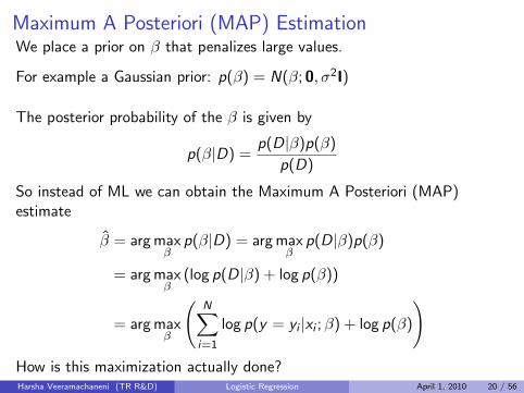
Maximum A Posteriori (MAP) EstimationWe place a prior on β that penalizes large values.
For example a Gaussian prior: p(β) = N(β; 0, σ2I)
The posterior probability of the β is given by
p(β|D) =p(D|β)p(β)
p(D)
So instead of ML we can obtain the Maximum A Posteriori (MAP)estimate
β̂ = arg maxβ
p(β|D) = arg maxβ
p(D|β)p(β)
= arg maxβ
(log p(D|β) + log p(β))
= arg maxβ
(N∑
i=1
log p(y = yi |xi ;β) + log p(β)
)How is this maximization actually done?Harsha Veeramachaneni (TR R&D) Logistic Regression April 1, 2010 20 / 56
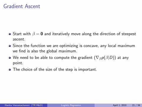
Gradient Ascent
Start with β = 0 and iteratively move along the direction of steepestascent.
Since the function we are optimizing is concave, any local maximumwe find is also the global maximum.
We need to be able to compute the gradient (∇βp(β|D)) at anypoint.
The choice of the size of the step is important.
Harsha Veeramachaneni (TR R&D) Logistic Regression April 1, 2010 21 / 56
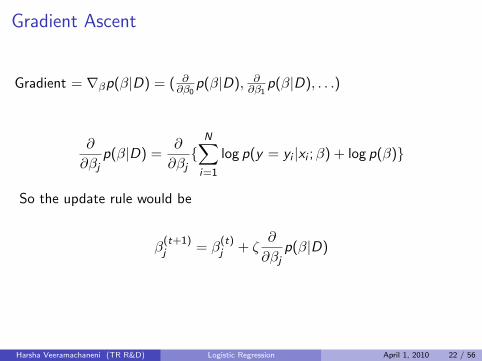
Gradient Ascent
Gradient = ∇βp(β|D) = ( ∂∂β0
p(β|D), ∂∂β1
p(β|D), . . .)
∂
∂βjp(β|D) =
∂
∂βj{
N∑i=1
log p(y = yi |xi ;β) + log p(β)}
So the update rule would be
β(t+1)j = β
(t)j + ζ
∂
∂βjp(β|D)
Harsha Veeramachaneni (TR R&D) Logistic Regression April 1, 2010 22 / 56
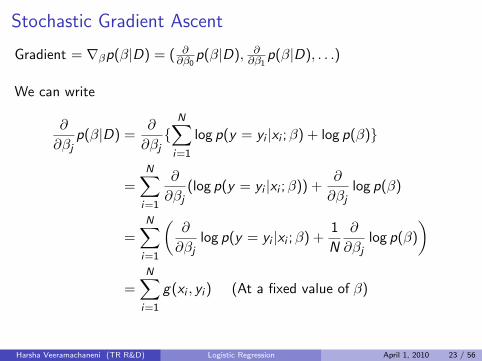
Stochastic Gradient Ascent
Gradient = ∇βp(β|D) = ( ∂∂β0
p(β|D), ∂∂β1
p(β|D), . . .)
We can write
∂
∂βjp(β|D) =
∂
∂βj{
N∑i=1
log p(y = yi |xi ;β) + log p(β)}
=N∑
i=1
∂
∂βj(log p(y = yi |xi ;β)) +
∂
∂βjlog p(β)
=N∑
i=1
(∂
∂βjlog p(y = yi |xi ;β) +
1
N
∂
∂βjlog p(β)
)
=N∑
i=1
g(xi , yi ) (At a fixed value of β)
Harsha Veeramachaneni (TR R&D) Logistic Regression April 1, 2010 23 / 56
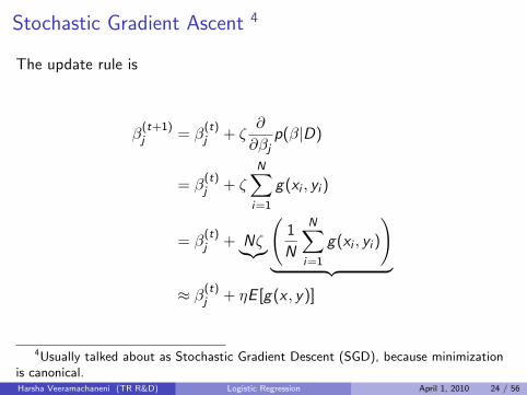
Stochastic Gradient Ascent 4
The update rule is
β(t+1)j = β
(t)j + ζ
∂
∂βjp(β|D)
= β(t)j + ζ
N∑i=1
g(xi , yi )
= β(t)j + Nζ︸︷︷︸
(1
N
N∑i=1
g(xi , yi )
)︸ ︷︷ ︸
≈ β(t)j + ηE [g(x , y)]
4Usually talked about as Stochastic Gradient Descent (SGD), because minimizationis canonical.Harsha Veeramachaneni (TR R&D) Logistic Regression April 1, 2010 24 / 56
Stochastic Gradient Ascent
We could randomly sample a small batch of L examples from thetraining set to estimate E [g(x , y)].
What if we went to extreme and made L = 1?
We obtain online (incremental) learning.
Can be shown to converge to the same optimum under somereasonable assumptions.
Harsha Veeramachaneni (TR R&D) Logistic Regression April 1, 2010 25 / 56
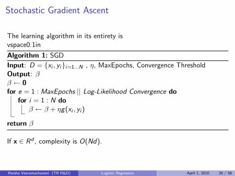
Stochastic Gradient Ascent
The learning algorithm in its entirety isvspace0.1in
Algorithm 1: SGD
Input: D = {xi , yi}i=1...N , η, MaxEpochs, Convergence ThresholdOutput: ββ ← 0for e = 1 : MaxEpochs || Log-Likelihood Convergence do
for i = 1 : N doβ ← β + ηg(xi , yi )
return β
If x ∈ Rd , complexity is O(Nd).
Harsha Veeramachaneni (TR R&D) Logistic Regression April 1, 2010 26 / 56
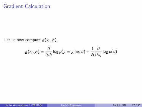
Gradient Calculation
Let us now compute g(xi , yi ).
g(xi , yi ) =∂
∂βjlog p(y = yi |xi ;β) +
1
N
∂
∂βjlog p(β)
Harsha Veeramachaneni (TR R&D) Logistic Regression April 1, 2010 27 / 56
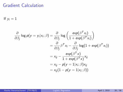
Gradient Calculation
If yi = 1
∂
∂βjlog p(y = yi |xi ;β) =
∂
∂βjlog
(exp(βT xi )
1 + exp(βT xi )
)=
∂
∂βjβT xi −
∂
∂βjlog(1 + exp(βT xi ))
= xij −exp(βT x)
1 + exp(βT x)xij
= xij − p(y = 1|xi ;β)xij
= xij(1− p(y = 1|xi ;β))
Harsha Veeramachaneni (TR R&D) Logistic Regression April 1, 2010 28 / 56
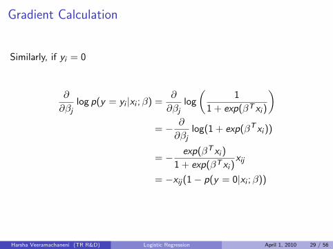
Gradient Calculation
Similarly, if yi = 0
∂
∂βjlog p(y = yi |xi ;β) =
∂
∂βjlog
(1
1 + exp(βT xi )
)= − ∂
∂βjlog(1 + exp(βT xi ))
= − exp(βT xi )
1 + exp(βT xi )xij
= −xij(1− p(y = 0|xi ;β))
Harsha Veeramachaneni (TR R&D) Logistic Regression April 1, 2010 29 / 56
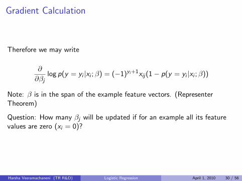
Gradient Calculation
Therefore we may write
∂
∂βjlog p(y = yi |xi ;β) = (−1)yi +1xij(1− p(y = yi |xi ;β))
Note: β is in the span of the example feature vectors. (RepresenterTheorem)
Question: How many βj will be updated if for an example all its featurevalues are zero (xi = 0)?
Harsha Veeramachaneni (TR R&D) Logistic Regression April 1, 2010 30 / 56

Lazy Update
If we ignore the prior,for each example, we only need to update the coordinates of β wherethe feature vector is non-zero.
Makes learning very fast if the feature vectors are sparse.
Complexity reduces to O(Ns), where s is the average number ofnon-zero feature values.
What happens when we add the prior?
Harsha Veeramachaneni (TR R&D) Logistic Regression April 1, 2010 31 / 56
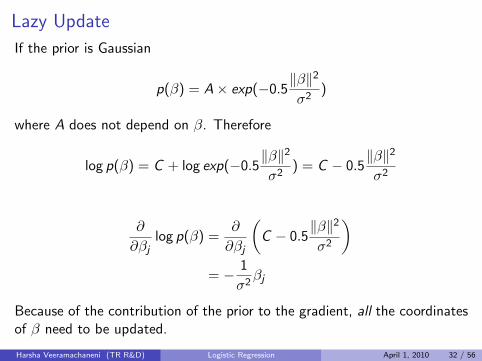
Lazy Update
If the prior is Gaussian
p(β) = A× exp(−0.5‖β‖2
σ2)
where A does not depend on β. Therefore
log p(β) = C + log exp(−0.5‖β‖2
σ2) = C − 0.5
‖β‖2
σ2
∂
∂βjlog p(β) =
∂
∂βj
(C − 0.5
‖β‖2
σ2
)= − 1
σ2βj
Because of the contribution of the prior to the gradient, all the coordinatesof β need to be updated.
Harsha Veeramachaneni (TR R&D) Logistic Regression April 1, 2010 32 / 56
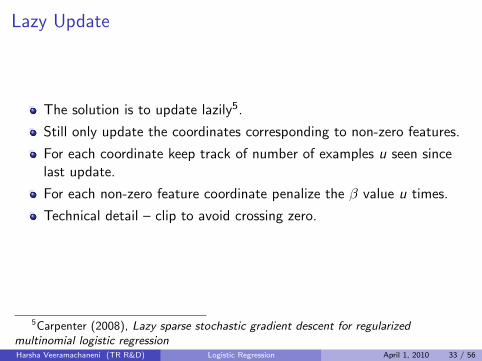
Lazy Update
The solution is to update lazily5.
Still only update the coordinates corresponding to non-zero features.
For each coordinate keep track of number of examples u seen sincelast update.
For each non-zero feature coordinate penalize the β value u times.
Technical detail – clip to avoid crossing zero.
5Carpenter (2008), Lazy sparse stochastic gradient descent for regularizedmultinomial logistic regressionHarsha Veeramachaneni (TR R&D) Logistic Regression April 1, 2010 33 / 56
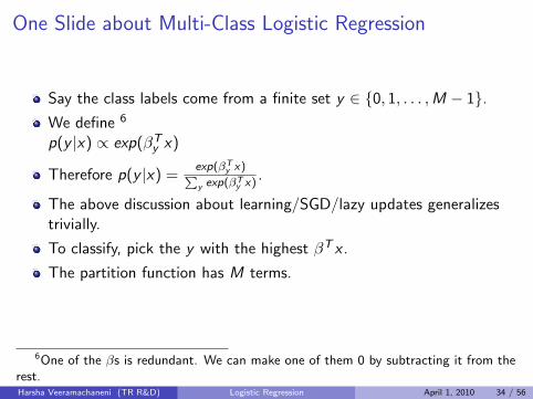
One Slide about Multi-Class Logistic Regression
Say the class labels come from a finite set y ∈ {0, 1, . . . ,M − 1}.We define 6
p(y |x) ∝ exp(βTy x)
Therefore p(y |x) =exp(βT
y x)Py exp(βT
y x).
The above discussion about learning/SGD/lazy updates generalizestrivially.
To classify, pick the y with the highest βT x .
The partition function has M terms.
6One of the βs is redundant. We can make one of them 0 by subtracting it from therest.Harsha Veeramachaneni (TR R&D) Logistic Regression April 1, 2010 34 / 56
1 Logistic Regression (Plain and Simple)Introduction to logistic regression
2 Learning AlgorithmLog-LikelihoodGradient DescentLazy Updates
3 Kernelization
4 Sequence Tagging
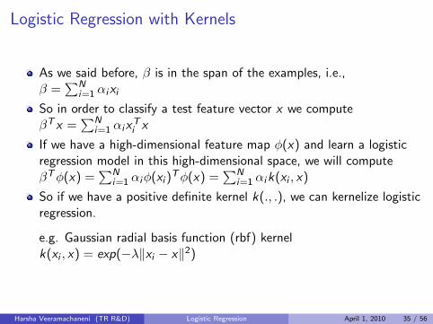
Logistic Regression with Kernels
As we said before, β is in the span of the examples, i.e.,β =
∑Ni=1 αixi
So in order to classify a test feature vector x we computeβT x =
∑Ni=1 αix
Ti x
If we have a high-dimensional feature map φ(x) and learn a logisticregression model in this high-dimensional space, we will computeβTφ(x) =
∑Ni=1 αiφ(xi )
Tφ(x) =∑N
i=1 αik(xi , x)
So if we have a positive definite kernel k(., .), we can kernelize logisticregression.
e.g. Gaussian radial basis function (rbf) kernelk(xi , x) = exp(−λ‖xi − x‖2)
Harsha Veeramachaneni (TR R&D) Logistic Regression April 1, 2010 35 / 56
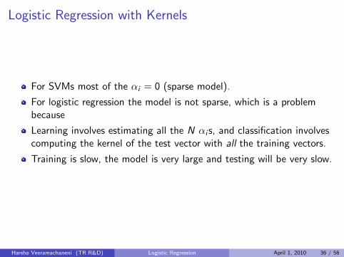
Logistic Regression with Kernels
For SVMs most of the αi = 0 (sparse model).
For logistic regression the model is not sparse, which is a problembecause
Learning involves estimating all the N αi s, and classification involvescomputing the kernel of the test vector with all the training vectors.
Training is slow, the model is very large and testing will be very slow.
Harsha Veeramachaneni (TR R&D) Logistic Regression April 1, 2010 36 / 56
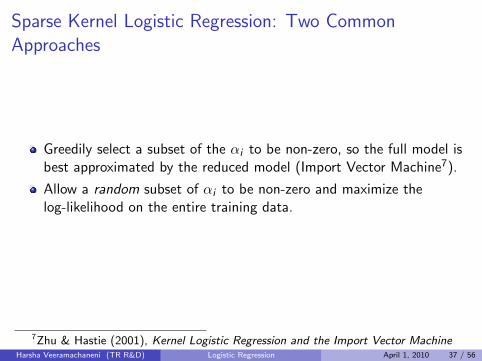
Sparse Kernel Logistic Regression: Two CommonApproaches
Greedily select a subset of the αi to be non-zero, so the full model isbest approximated by the reduced model (Import Vector Machine7).
Allow a random subset of αi to be non-zero and maximize thelog-likelihood on the entire training data.
7Zhu & Hastie (2001), Kernel Logistic Regression and the Import Vector MachineHarsha Veeramachaneni (TR R&D) Logistic Regression April 1, 2010 37 / 56
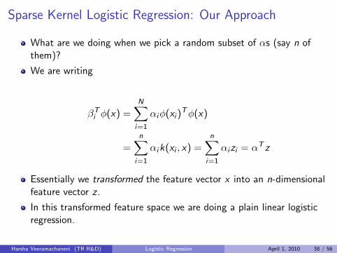
Sparse Kernel Logistic Regression: Our Approach
What are we doing when we pick a random subset of αs (say n ofthem)?
We are writing
βTi φ(x) =
N∑i=1
αiφ(xi )Tφ(x)
=n∑
i=1
αik(xi , x) =n∑
i=1
αizi = αT z
Essentially we transformed the feature vector x into an n-dimensionalfeature vector z .
In this transformed feature space we are doing a plain linear logisticregression.
Harsha Veeramachaneni (TR R&D) Logistic Regression April 1, 2010 38 / 56
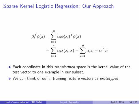
Sparse Kernel Logistic Regression: Our Approach
βTi φ(x) =
N∑i=1
αiφ(xi )Tφ(x)
=n∑
i=1
αik(xi , x) =n∑
i=1
αizi = αT zi
Each coordinate in this transformed space is the kernel value of thetest vector to one example in our subset.
We can think of our n training feature vectors as prototypes
Harsha Veeramachaneni (TR R&D) Logistic Regression April 1, 2010 39 / 56
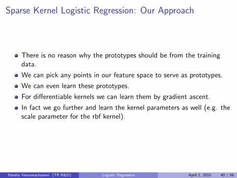
Sparse Kernel Logistic Regression: Our Approach
There is no reason why the prototypes should be from the trainingdata.
We can pick any points in our feature space to serve as prototypes.
We can even learn these prototypes.
For differentiable kernels we can learn them by gradient ascent.
In fact we go further and learn the kernel parameters as well (e.g. thescale parameter for the rbf kernel).
Harsha Veeramachaneni (TR R&D) Logistic Regression April 1, 2010 40 / 56
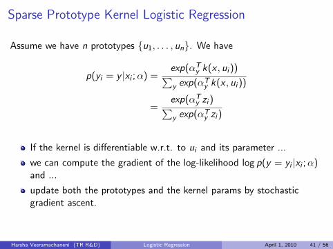
Sparse Prototype Kernel Logistic Regression
Assume we have n prototypes {u1, . . . , un}. We have
p(yi = y |xi ;α) =exp(αT
y k(x , ui ))∑y exp(αT
y k(x , ui ))
=exp(αT
y zi )∑y exp(αT
y zi )
If the kernel is differentiable w.r.t. to ui and its parameter ...
we can compute the gradient of the log-likelihood log p(y = yi |xi ;α)and ...
update both the prototypes and the kernel params by stochasticgradient ascent.
Harsha Veeramachaneni (TR R&D) Logistic Regression April 1, 2010 41 / 56
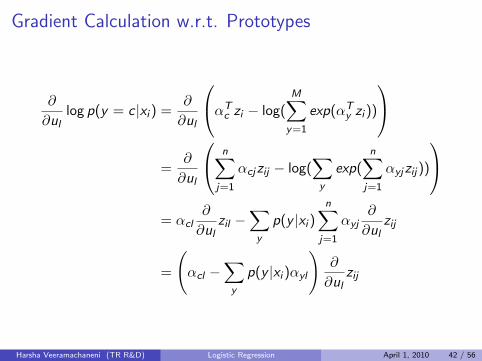
Gradient Calculation w.r.t. Prototypes
∂
∂ullog p(y = c |xi ) =
∂
∂ul
αTc zi − log(
M∑y=1
exp(αTy zi ))
=
∂
∂ul
n∑j=1
αcjzij − log(∑y
exp(n∑
j=1
αyjzij))
= αcl
∂
∂ulzil −
∑y
p(y |xi )n∑
j=1
αyj∂
∂ulzij
=
(αcl −
∑y
p(y |xi )αyl
)∂
∂ulzij
Harsha Veeramachaneni (TR R&D) Logistic Regression April 1, 2010 42 / 56
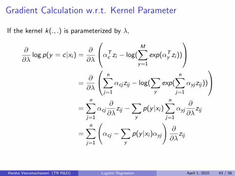
Gradient Calculation w.r.t. Kernel Parameter
If the kernel k(., .) is parameterized by λ,
∂
∂λlog p(y = c |xi ) =
∂
∂λ
αTc zi − log(
M∑y=1
exp(αTy zi ))
=
∂
∂λ
n∑j=1
αcjzij − log(∑y
exp(n∑
j=1
αyjzij))
=
n∑j=1
αcj∂
∂λzij −
∑y
p(y |xi )n∑
j=1
αyj∂
∂λzij
=n∑
j=1
(αcj −
∑y
p(y |xi )αyj
)∂
∂λzij
Harsha Veeramachaneni (TR R&D) Logistic Regression April 1, 2010 43 / 56

Gradient Calculation – Gaussian Radial Basis FunctionKernel
For the Gaussian r.b.f. kernel zil = k(xi , ul) = exp(−λ‖xi − ul‖2).
∂
∂ulzij =
∂
∂ulexp(−λ‖xi − ul‖2)
= 2λ(xi − ul)zil
∂
∂λzij =
∂
∂λexp(−λ‖xi − ul‖2)
= −‖xi − ul‖2zil
Harsha Veeramachaneni (TR R&D) Logistic Regression April 1, 2010 44 / 56
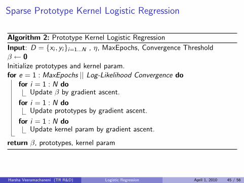
Sparse Prototype Kernel Logistic Regression
Algorithm 2: Prototype Kernel Logistic Regression
Input: D = {xi , yi}i=1...N , η, MaxEpochs, Convergence Thresholdβ ← 0Initialize prototypes and kernel param.for e = 1 : MaxEpochs || Log-Likelihood Convergence do
for i = 1 : N doUpdate β by gradient ascent.
for i = 1 : N doUpdate prototypes by gradient ascent.
for i = 1 : N doUpdate kernel param by gradient ascent.
return β, prototypes, kernel param
Harsha Veeramachaneni (TR R&D) Logistic Regression April 1, 2010 45 / 56
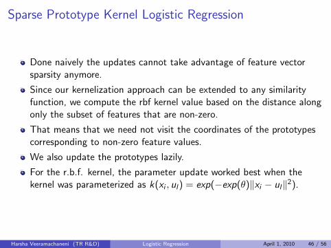
Sparse Prototype Kernel Logistic Regression
Done naively the updates cannot take advantage of feature vectorsparsity anymore.
Since our kernelization approach can be extended to any similarityfunction, we compute the rbf kernel value based on the distance alongonly the subset of features that are non-zero.
That means that we need not visit the coordinates of the prototypescorresponding to non-zero feature values.
We also update the prototypes lazily.
For the r.b.f. kernel, the parameter update worked best when thekernel was parameterized as k(xi , ul) = exp(−exp(θ)‖xi − ul‖2).
Harsha Veeramachaneni (TR R&D) Logistic Regression April 1, 2010 46 / 56

Demo Here
Harsha Veeramachaneni (TR R&D) Logistic Regression April 1, 2010 47 / 56
1 Logistic Regression (Plain and Simple)Introduction to logistic regression
2 Learning AlgorithmLog-LikelihoodGradient DescentLazy Updates
3 Kernelization
4 Sequence Tagging
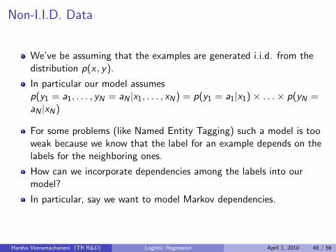
Non-I.I.D. Data
We’ve be assuming that the examples are generated i.i.d. from thedistribution p(x , y).
In particular our model assumesp(y1 = a1, . . . , yN = aN |x1, . . . , xN) = p(y1 = a1|x1)× . . .× p(yN =aN |xN)
For some problems (like Named Entity Tagging) such a model is tooweak because we know that the label for an example depends on thelabels for the neighboring ones.
How can we incorporate dependencies among the labels into ourmodel?
In particular, say we want to model Markov dependencies.
Harsha Veeramachaneni (TR R&D) Logistic Regression April 1, 2010 48 / 56
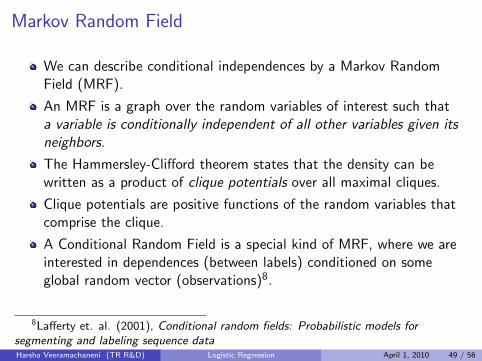
Markov Random Field
We can describe conditional independences by a Markov RandomField (MRF).
An MRF is a graph over the random variables of interest such thata variable is conditionally independent of all other variables given itsneighbors.
The Hammersley-Clifford theorem states that the density can bewritten as a product of clique potentials over all maximal cliques.
Clique potentials are positive functions of the random variables thatcomprise the clique.
A Conditional Random Field is a special kind of MRF, where we areinterested in dependences (between labels) conditioned on someglobal random vector (observations)8.
8Lafferty et. al. (2001), Conditional random fields: Probabilistic models forsegmenting and labeling sequence dataHarsha Veeramachaneni (TR R&D) Logistic Regression April 1, 2010 49 / 56
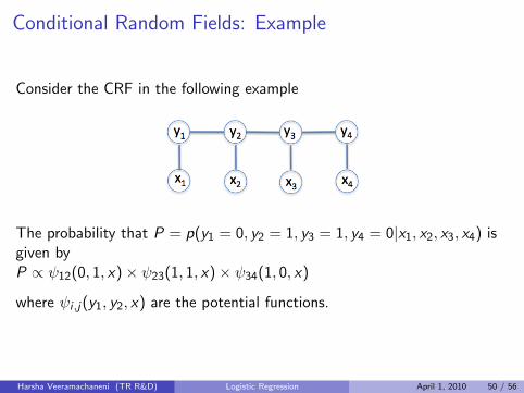
Conditional Random Fields: Example
Consider the CRF in the following example
The probability that P = p(y1 = 0, y2 = 1, y3 = 1, y4 = 0|x1, x2, x3, x4) isgiven byP ∝ ψ12(0, 1, x)× ψ23(1, 1, x)× ψ34(1, 0, x)
where ψi ,j(y1, y2, x) are the potential functions.
Harsha Veeramachaneni (TR R&D) Logistic Regression April 1, 2010 50 / 56
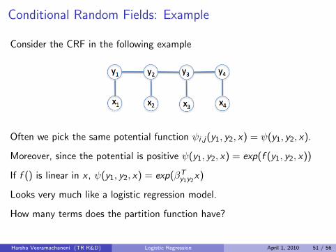
Conditional Random Fields: Example
Consider the CRF in the following example
Often we pick the same potential function ψi ,j(y1, y2, x) = ψ(y1, y2, x).
Moreover, since the potential is positive ψ(y1, y2, x) = exp(f (y1, y2, x))
If f () is linear in x , ψ(y1, y2, x) = exp(βTy1y2
x)
Looks very much like a logistic regression model.
How many terms does the partition function have?
Harsha Veeramachaneni (TR R&D) Logistic Regression April 1, 2010 51 / 56
Learning and Decoding for CRFs
To learn CRFs by gradient descent, we need to compute thederivative of the log-likelihood.
Again the derivative involves the partition function.
The calculation of the partition function is efficient for chain CRFs(forward-backward algorithm).
Although MALLET uses L-BFGS, CRFs can also be learned bystochastic gradient descent.
For chain CRFs decoding can be done efficiently by dynamicprogramming (Viterbi algorithm).
Harsha Veeramachaneni (TR R&D) Logistic Regression April 1, 2010 52 / 56

Viterbi Decoding
The weight on the arrows represents the benefit of transitioning fromthe previous label to the current label for that particular token.
It is the logarithm of the potential function value for that clique(βT
y1y2x).
To decode, we find the path with the maximum benefit by dynamicprogramming.
Harsha Veeramachaneni (TR R&D) Logistic Regression April 1, 2010 53 / 56
Sequence Tagging without CRFs
We can use Viterbi decoding without the additional cost offorward-backward at training time by just learning a logistic regressionto pairs of classes.
The training sequence data is used to assign a class-pair label to eachexample.
The class-pair model is smoothed with a single class model.
At decoding time pretend that the model was learned under a CRFassumption.
Often gives a better model because the assumption made by CRFsthat the training sequences are drawn i.i.d. is violated.
Harsha Veeramachaneni (TR R&D) Logistic Regression April 1, 2010 54 / 56
Sequence Tagging using Logistic Regression
Our approach gives similar (and sometimes better) accuracy for NERthan CRFs (MALLET).
Our un-optimized implementation trains 30-50 times faster.
The code is being used in projects requiring incremental learning.
The barrier for implementing active learning systems is now muchlower.
Harsha Veeramachaneni (TR R&D) Logistic Regression April 1, 2010 55 / 56

Current and Near Term
Minimax & Type-specific Priors for domain independence.
Active Learning
Ranking
Semi-Supervised
....
Harsha Veeramachaneni (TR R&D) Logistic Regression April 1, 2010 56 / 56


![Pointwise HSIC: A Linear-Time Kernelized Co-occurrence ...yokoi/docs/yokoi-phsic-slide...Pointwise HSIC: A Linear-Time Kernelized Co-occurrence Norm for Sparse Linguistic Expressions[EMNLP2018]](https://cdn.vdocuments.mx/doc/165x107/60ea8bad015b200d936ab56e/pointwise-hsic-a-linear-time-kernelized-co-occurrence-yokoidocsyokoi-phsic-slide.jpg)


