
Lecture 11: Logistic Regression III—Ordered Data
Prof. Sharyn O’Halloran Sustainable Development U9611Econometrics II
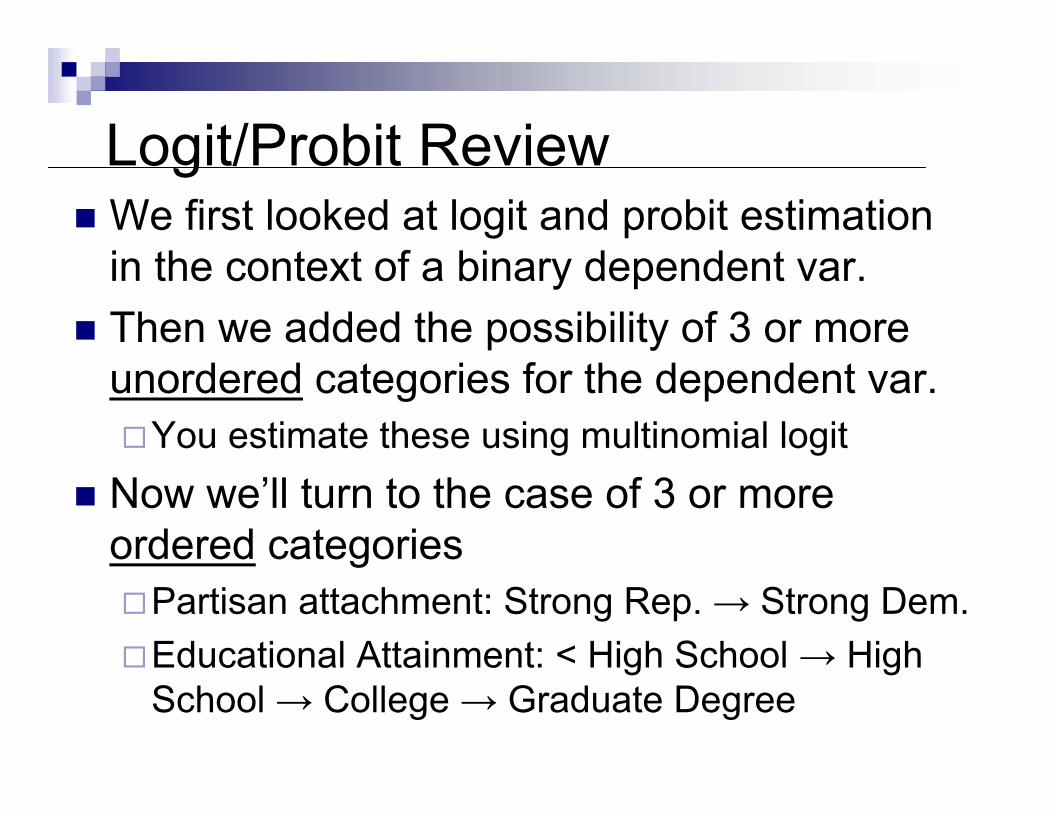
Logit/Probit ReviewWe first looked at logit and probit estimation in the context of a binary dependent var.Then we added the possibility of 3 or more unordered categories for the dependent var.
You estimate these using multinomial logitNow we’ll turn to the case of 3 or more ordered categories
Partisan attachment: Strong Rep. → Strong Dem.Educational Attainment: < High School → High School → College → Graduate Degree

Binary Probit Estimation
•Binary dependent variable Y = 0 or 1 (e.g., elect Democrat or Republican)•Estimate Probit(Y) = β0 + x1*β1 + x2*β2 + … with Stata, get β coefficients •Calculate Xiβ = β0 + x1i*β1 + x2i=*β2 + … for each observation
0.1
.2.3
.4
- 4 -2 0 2 4
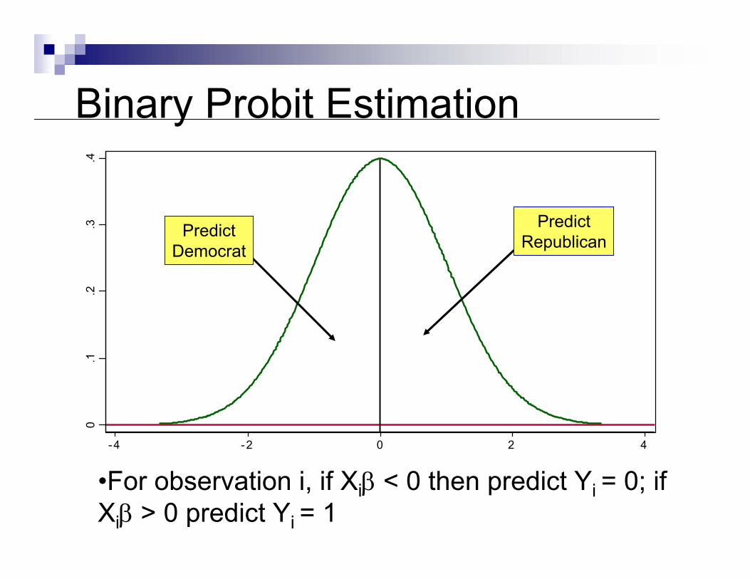
•For observation i, if Xiβ < 0 then predict Yi = 0; if Xiβ > 0 predict Yi = 1
Binary Probit Estimation0
.1.2
.3.4
- 4 -2 0 2 4
PredictRepublicanPredict
Democrat
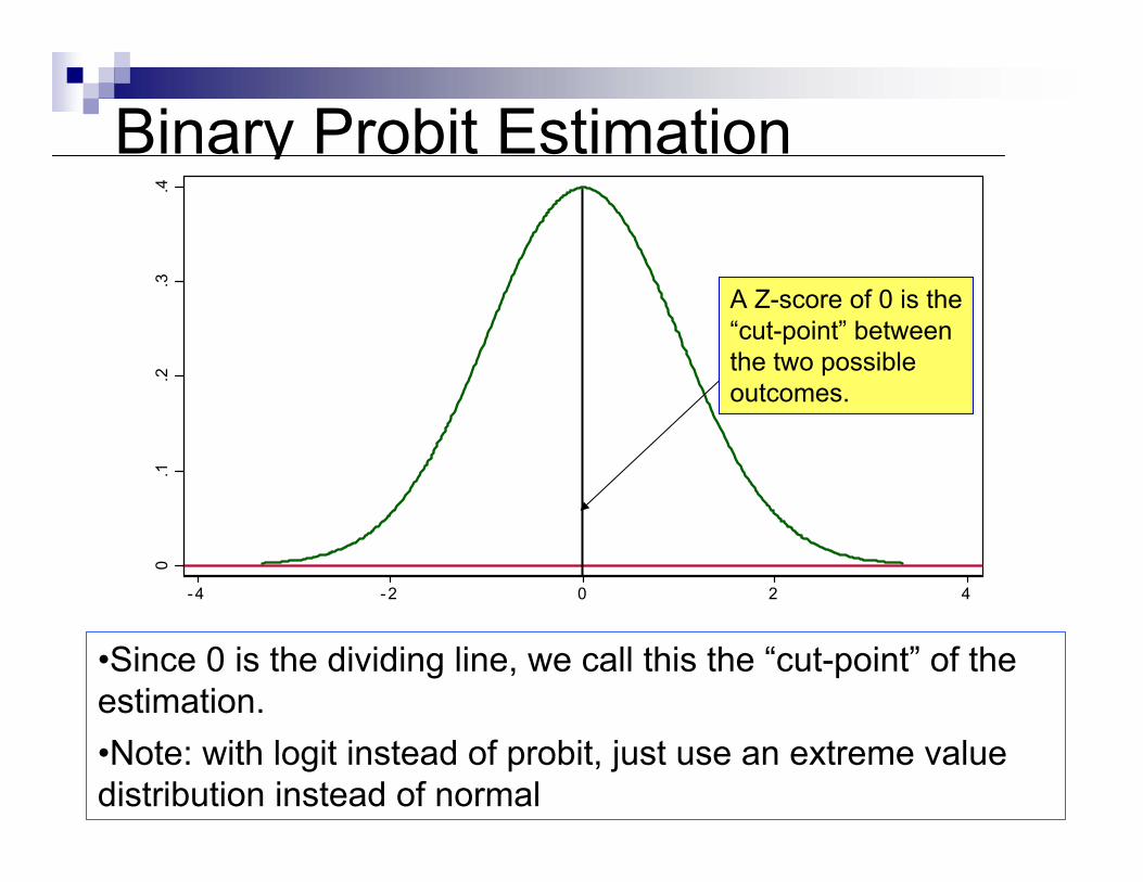
Binary Probit Estimation
•Since 0 is the dividing line, we call this the “cut-point” of the estimation.•Note: with logit instead of probit, just use an extreme value distribution instead of normal
0.1
.2.3
.4
- 4 -2 0 2 4
A Z-score of 0 is the“cut-point” betweenthe two possibleoutcomes.

Binary Probit Estimation
■ Interpretation of β1: increasing x1 by one unit changes the Z-score by β1 units
■ The impact of this on Prob(Y=1) depends on your starting point
0.1
.2.3
.4
- 4 -2 0 2 4
Binary Probit Estimation
■ Interpretation of β1: increasing x1 by one unit changes the Z-score by β1units
■ The impact of this on Prob(Y=1) depends on your starting point
0.1
.2.3
.4
- 4 -2 0 2 4β1
∆1
Z-Score
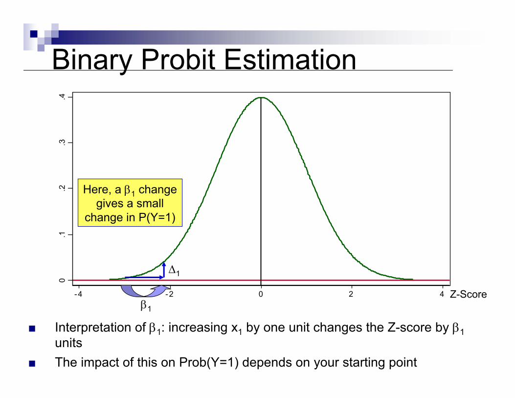
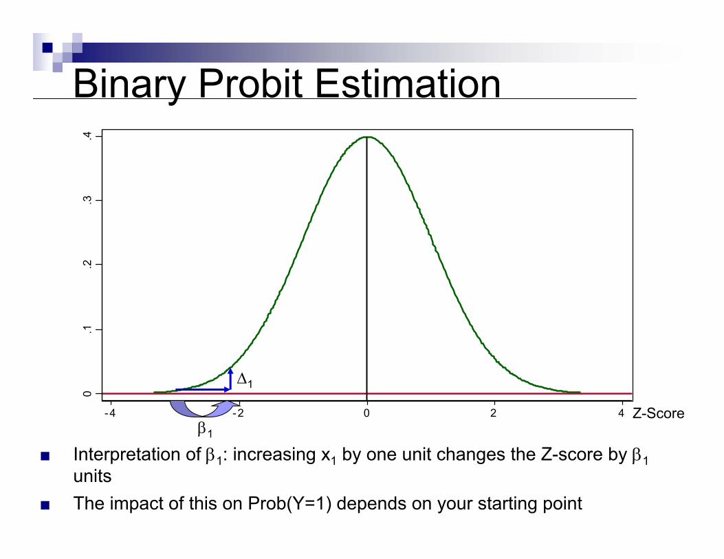
Binary Probit Estimation
■ Interpretation of β1: increasing x1 by one unit changes the Z-score by β1units
■ The impact of this on Prob(Y=1) depends on your starting point
0.1
.2.3
.4
- 4 -2 0 2 4β1
∆1
Z-Score
Here, a β1 changegives a small
change in P(Y=1)
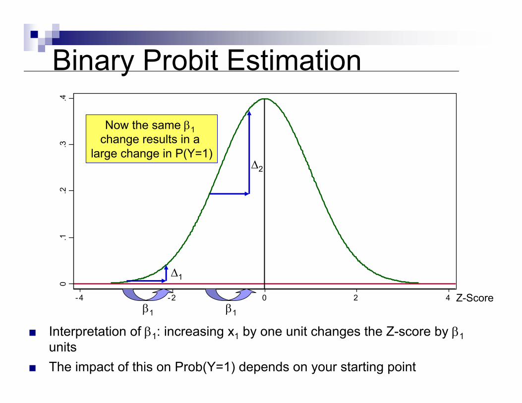
Binary Probit Estimation
■ Interpretation of β1: increasing x1 by one unit changes the Z-score by β1units
■ The impact of this on Prob(Y=1) depends on your starting point
0.1
.2.3
.4
- 4 -2 0 2 4β1 β1
∆1
∆2
Z-Score
Now the same β1change results in a
large change in P(Y=1)

Ordered Probit Estimation0
.1.2
.3.4
- 4 -2 0 2 4
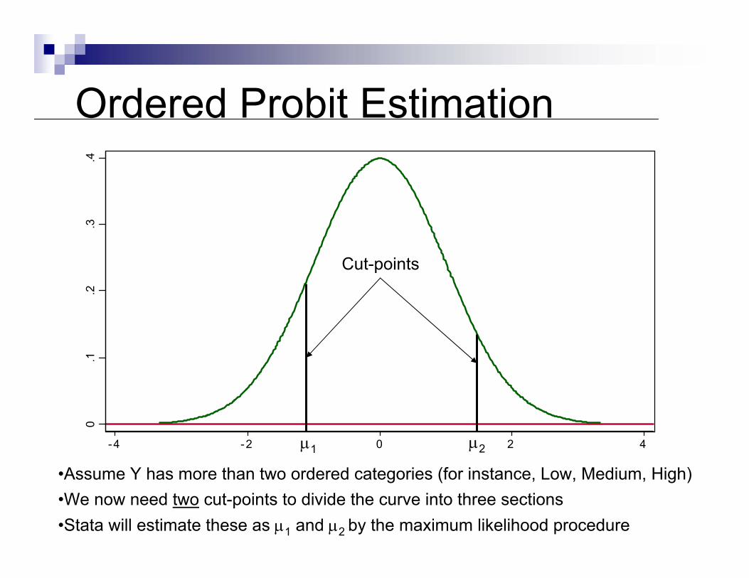
■ Assume Y has more than two ordered categories (for instance, Low, Medium, High)
■ We now need two cut-points to divide the curve into three sections■ Stata will estimate these as µ1 and µ2 by the maximum likelihood procedure
Ordered Probit Estimation0
.1.2
.3.4
- 4 -2 0 2 4µ1 µ2
Cut-points
•Assume Y has more than two ordered categories (for instance, Low, Medium, High)•We now need two cut-points to divide the curve into three sections•Stata will estimate these as µ1 and µ2 by the maximum likelihood procedure

Ordered Probit Estimation0
.1.2
.3.4
- 4 -2 0 2 4µ1 µ2
PredictLow
PredictHigh
PredictMedium
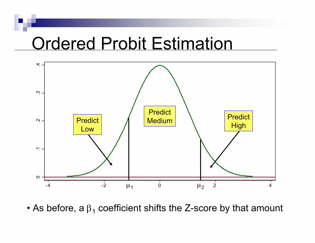
• If Xiβ < µ1 then predict Yi = Low • If µ1 < Xiβ < µ2 then predict Yi = Medium• If Xiβ > µ2 then predict Yi = High
0.1
.2.3
.4
- 4 -2 0 2 4µ1 µ2
PredictLow
PredictHigh
PredictMedium
Ordered Probit Estimation
• As before, a β1 coefficient shifts the Z-score by that amount
0.1
.2.3
.4
- 4 -2 0 2 4µ1 µ2
PredictLow
PredictHigh
PredictMedium
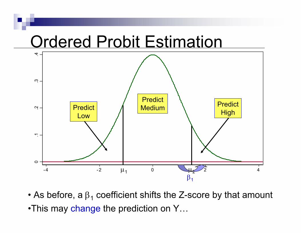
Ordered Probit Estimation
• As before, a β1 coefficient shifts the Z-score by that amount•This may change the prediction on Y…
β1
0.1
.2.3
.4
- 4 -2 0 2 4µ1 µ2
PredictLow
PredictHigh
PredictMedium
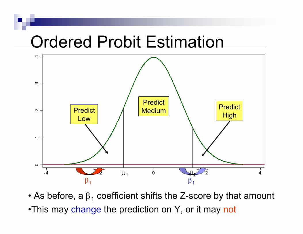
Ordered Probit Estimation
• As before, a β1 coefficient shifts the Z-score by that amount•This may change the prediction on Y, or it may not
β1 β1
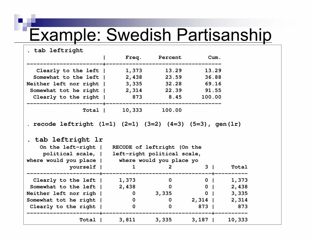
Example: Swedish Partisanship. tab leftright
| Freq. Percent Cum.-----------------------+-----------------------------------
Clearly to the left | 1,373 13.29 13.29Somewhat to the left | 2,438 23.59 36.88
Neither left nor right | 3,335 32.28 69.16Somewhat tot he right | 2,314 22.39 91.55Clearly to the right | 873 8.45 100.00
-----------------------+-----------------------------------Total | 10,333 100.00
. recode leftright (1=1) (2=1) (3=2) (4=3) (5=3), gen(lr)
. tab leftright lrOn the left-right | RECODE of leftright (On thepolitical scale, | left-right political scale,
where would you place | where would you place yoyourself | 1 2 3 | Total
----------------------+---------------------------------+----------Clearly to the left | 1,373 0 0 | 1,373
Somewhat to the left | 2,438 0 0 | 2,438 Neither left nor righ | 0 3,335 0 | 3,335 Somewhat tot he right | 0 0 2,314 | 2,314 Clearly to the right | 0 0 873 | 873
----------------------+---------------------------------+----------Total | 3,811 3,335 3,187 | 10,333
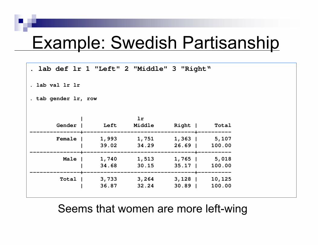
Example: Swedish Partisanship. lab def lr 1 "Left" 2 "Middle" 3 "Right“
. lab val lr lr
. tab gender lr, row
| lrGender | Left Middle Right | Total
---------------+---------------------------------+----------Female | 1,993 1,751 1,363 | 5,107
| 39.02 34.29 26.69 | 100.00 ---------------+---------------------------------+----------
Male | 1,740 1,513 1,765 | 5,018 | 34.68 30.15 35.17 | 100.00
---------------+---------------------------------+----------Total | 3,733 3,264 3,128 | 10,125
| 36.87 32.24 30.89 | 100.00
Seems that women are more left-wing
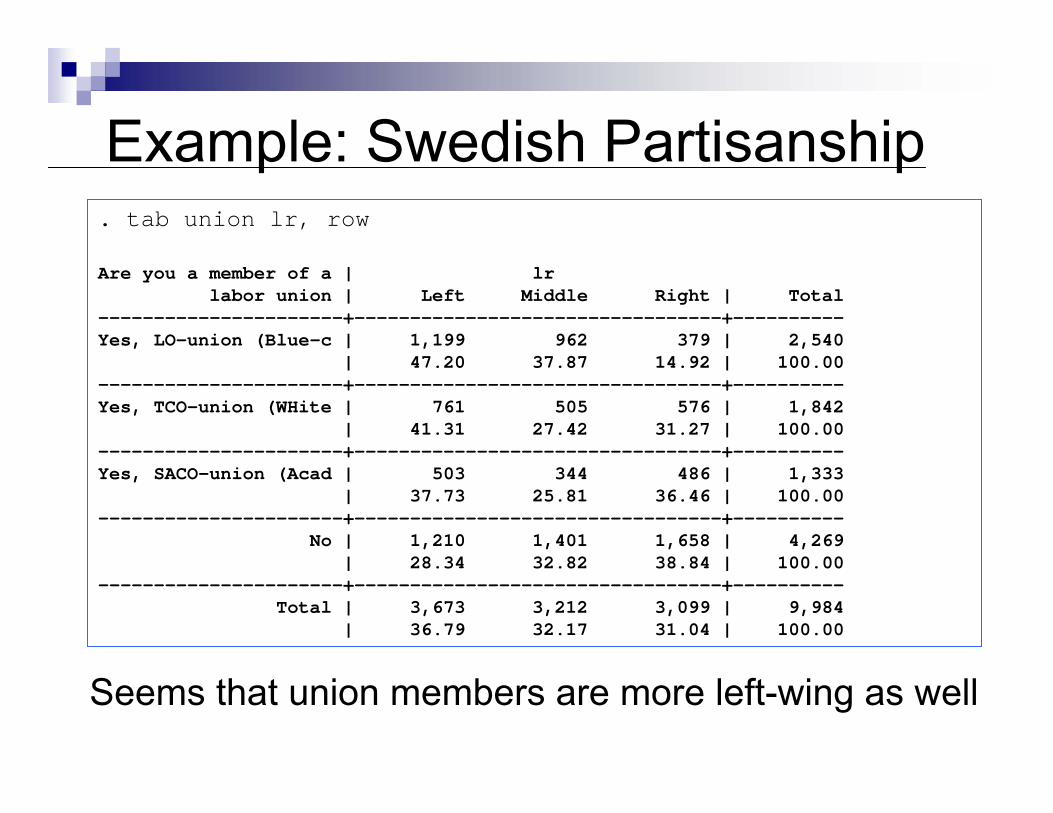
Example: Swedish Partisanship. tab union lr, row
Are you a member of a | lrlabor union | Left Middle Right | Total
----------------------+---------------------------------+----------Yes, LO-union (Blue-c | 1,199 962 379 | 2,540
| 47.20 37.87 14.92 | 100.00 ----------------------+---------------------------------+----------Yes, TCO-union (WHite | 761 505 576 | 1,842
| 41.31 27.42 31.27 | 100.00 ----------------------+---------------------------------+----------Yes, SACO-union (Acad | 503 344 486 | 1,333
| 37.73 25.81 36.46 | 100.00 ----------------------+---------------------------------+----------
No | 1,210 1,401 1,658 | 4,269 | 28.34 32.82 38.84 | 100.00
----------------------+---------------------------------+----------Total | 3,673 3,212 3,099 | 9,984
| 36.79 32.17 31.04 | 100.00
Seems that union members are more left-wing as well
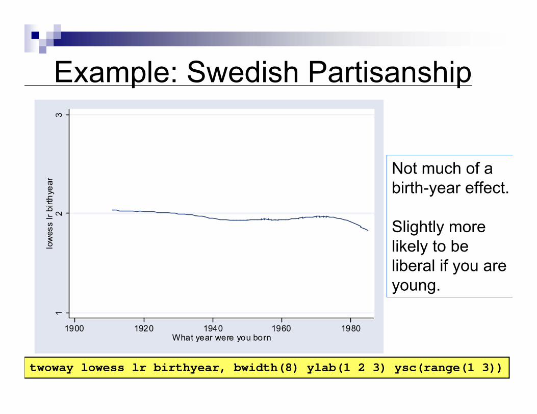
Example: Swedish Partisanship
twoway lowess lr birthyear, bwidth(8) ylab(1 2 3) ysc(range(1 3))
12
3lo
wes
s lr
birth
year
1900 1920 1940 1960 1980What year were you born
Not much of abirth-year effect.
Slightly more likely to beliberal if you areyoung.
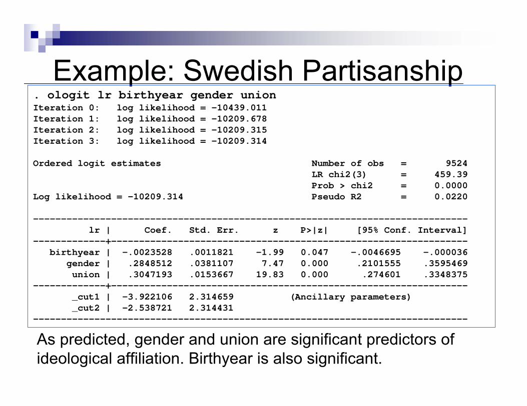
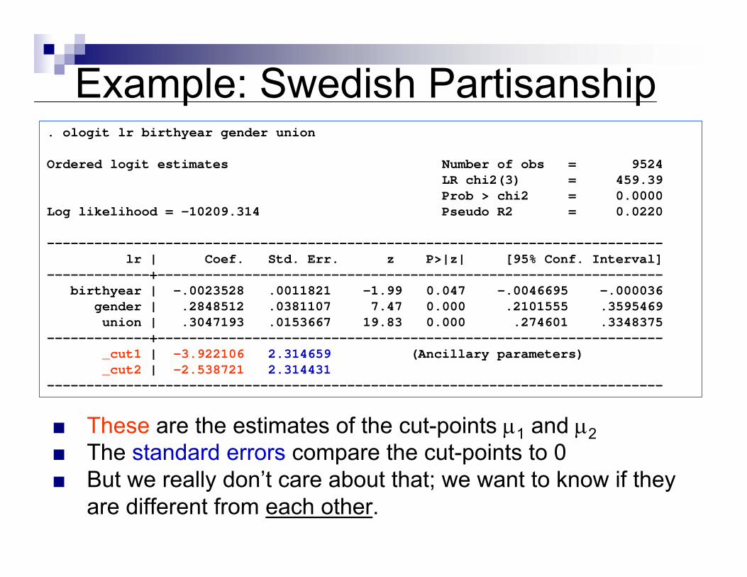
Example: Swedish Partisanship. ologit lr birthyear gender unionIteration 0: log likelihood = -10439.011Iteration 1: log likelihood = -10209.678Iteration 2: log likelihood = -10209.315Iteration 3: log likelihood = -10209.314
Ordered logit estimates Number of obs = 9524LR chi2(3) = 459.39Prob > chi2 = 0.0000
Log likelihood = -10209.314 Pseudo R2 = 0.0220
------------------------------------------------------------------------------lr | Coef. Std. Err. z P>|z| [95% Conf. Interval]
-------------+----------------------------------------------------------------birthyear | -.0023528 .0011821 -1.99 0.047 -.0046695 -.000036
gender | .2848512 .0381107 7.47 0.000 .2101555 .3595469union | .3047193 .0153667 19.83 0.000 .274601 .3348375
-------------+----------------------------------------------------------------_cut1 | -3.922106 2.314659 (Ancillary parameters)_cut2 | -2.538721 2.314431
------------------------------------------------------------------------------
As predicted, gender and union are significant predictors of ideological affiliation. Birthyear is also significant.
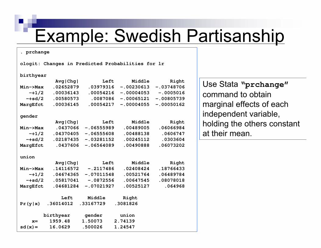
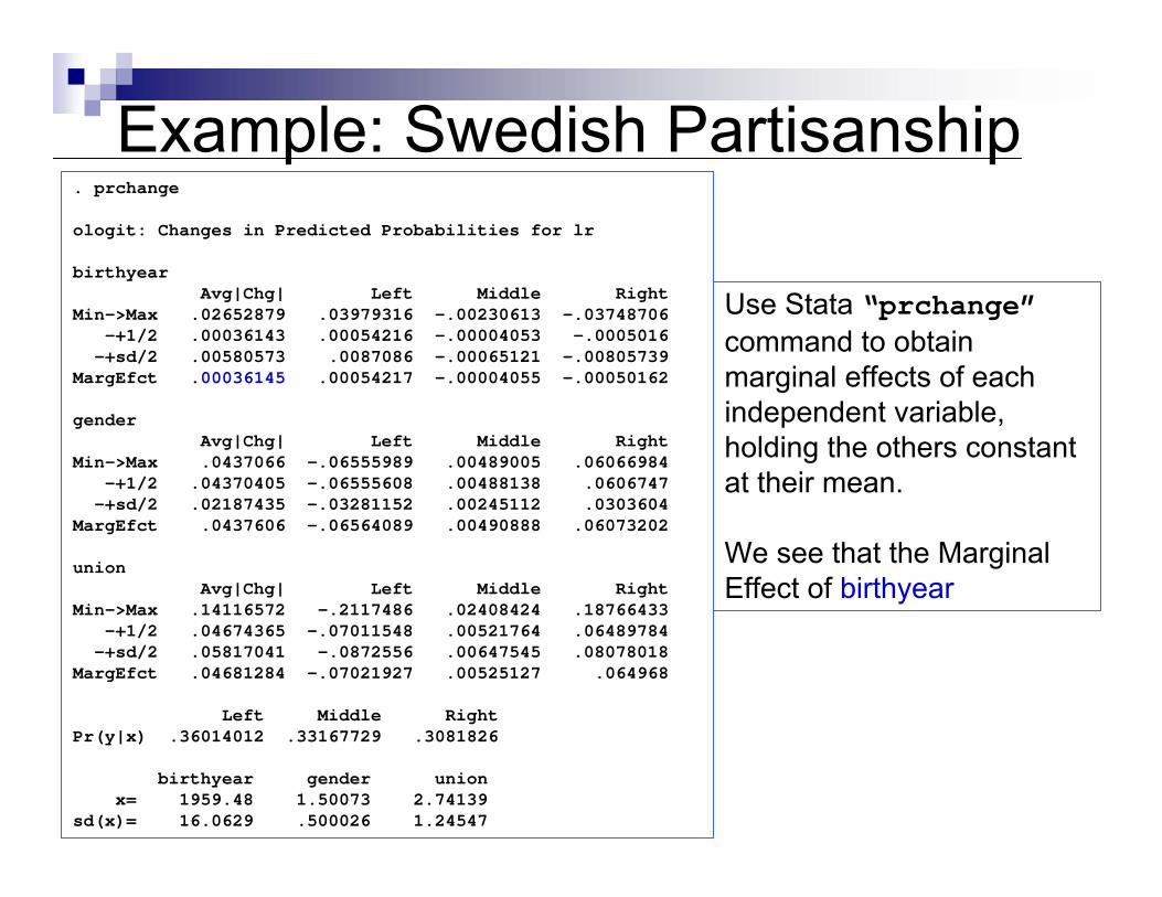
Example: Swedish Partisanship. prchange
ologit: Changes in Predicted Probabilities for lr
birthyearAvg|Chg| Left Middle Right
Min->Max .02652879 .03979316 -.00230613 -.03748706-+1/2 .00036143 .00054216 -.00004053 -.0005016
-+sd/2 .00580573 .0087086 -.00065121 -.00805739MargEfct .00036145 .00054217 -.00004055 -.00050162
genderAvg|Chg| Left Middle Right
Min->Max .0437066 -.06555989 .00489005 .06066984-+1/2 .04370405 -.06555608 .00488138 .0606747-+sd/2 .02187435 -.03281152 .00245112 .0303604
MargEfct .0437606 -.06564089 .00490888 .06073202
unionAvg|Chg| Left Middle Right
Min->Max .14116572 -.2117486 .02408424 .18766433-+1/2 .04674365 -.07011548 .00521764 .06489784
-+sd/2 .05817041 -.0872556 .00647545 .08078018MargEfct .04681284 -.07021927 .00525127 .064968
Left Middle RightPr(y|x) .36014012 .33167729 .3081826
birthyear gender unionx= 1959.48 1.50073 2.74139
sd(x)= 16.0629 .500026 1.24547
Use Stata “prchange”command to obtain marginal effects of each independent variable, holding the others constant at their mean.
We see that the Marginal Effect of birthyear
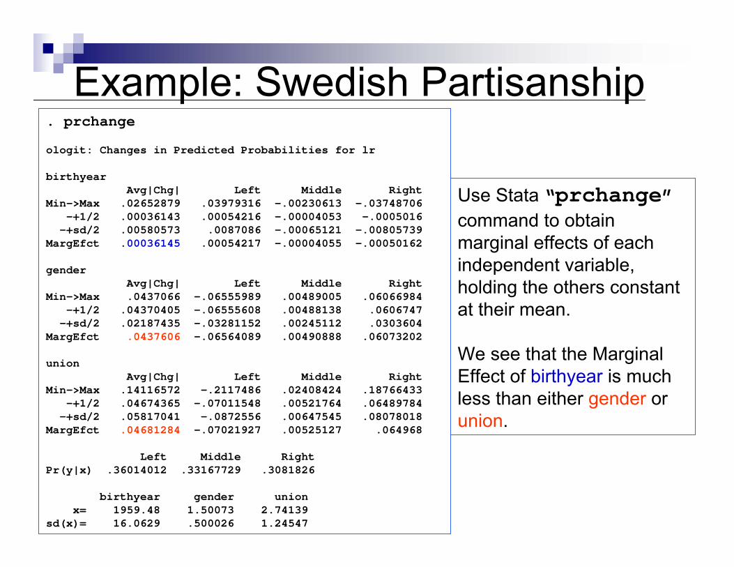
Example: Swedish Partisanship. prchange
ologit: Changes in Predicted Probabilities for lr
birthyearAvg|Chg| Left Middle Right
Min->Max .02652879 .03979316 -.00230613 -.03748706-+1/2 .00036143 .00054216 -.00004053 -.0005016
-+sd/2 .00580573 .0087086 -.00065121 -.00805739MargEfct .00036145 .00054217 -.00004055 -.00050162
genderAvg|Chg| Left Middle Right
Min->Max .0437066 -.06555989 .00489005 .06066984-+1/2 .04370405 -.06555608 .00488138 .0606747-+sd/2 .02187435 -.03281152 .00245112 .0303604
MargEfct .0437606 -.06564089 .00490888 .06073202
unionAvg|Chg| Left Middle Right
Min->Max .14116572 -.2117486 .02408424 .18766433-+1/2 .04674365 -.07011548 .00521764 .06489784
-+sd/2 .05817041 -.0872556 .00647545 .08078018MargEfct .04681284 -.07021927 .00525127 .064968
Left Middle RightPr(y|x) .36014012 .33167729 .3081826
birthyear gender unionx= 1959.48 1.50073 2.74139
sd(x)= 16.0629 .500026 1.24547
Use Stata “prchange”command to obtain marginal effects of each independent variable, holding the others constant at their mean.
We see that the Marginal Effect of birthyear is much less than either gender or union.
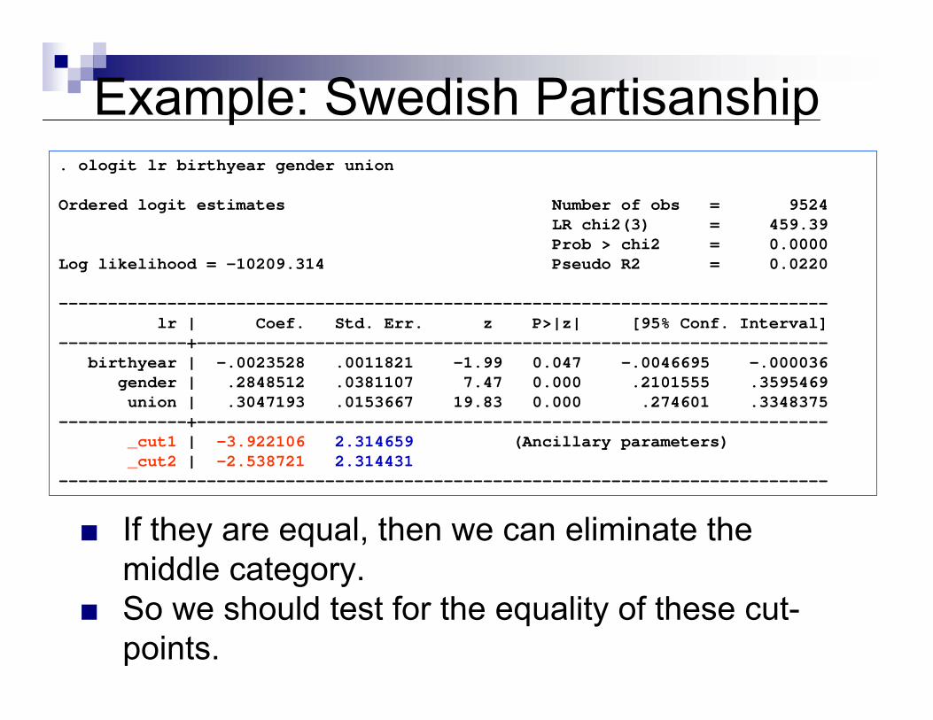
Example: Swedish Partisanship. ologit lr birthyear gender union
Ordered logit estimates Number of obs = 9524LR chi2(3) = 459.39Prob > chi2 = 0.0000
Log likelihood = -10209.314 Pseudo R2 = 0.0220
------------------------------------------------------------------------------lr | Coef. Std. Err. z P>|z| [95% Conf. Interval]
-------------+----------------------------------------------------------------birthyear | -.0023528 .0011821 -1.99 0.047 -.0046695 -.000036
gender | .2848512 .0381107 7.47 0.000 .2101555 .3595469union | .3047193 .0153667 19.83 0.000 .274601 .3348375
-------------+----------------------------------------------------------------_cut1 | -3.922106 2.314659 (Ancillary parameters)_cut2 | -2.538721 2.314431
------------------------------------------------------------------------------
■ These are the estimates of the cut-points µ1 and µ2■ The standard errors compare the cut-points to 0■ But we really don’t care about that; we want to know if they
are different from each other.
Example: Swedish Partisanship. ologit lr birthyear gender union
Ordered logit estimates Number of obs = 9524LR chi2(3) = 459.39Prob > chi2 = 0.0000
Log likelihood = -10209.314 Pseudo R2 = 0.0220
------------------------------------------------------------------------------lr | Coef. Std. Err. z P>|z| [95% Conf. Interval]
-------------+----------------------------------------------------------------birthyear | -.0023528 .0011821 -1.99 0.047 -.0046695 -.000036
gender | .2848512 .0381107 7.47 0.000 .2101555 .3595469union | .3047193 .0153667 19.83 0.000 .274601 .3348375
-------------+----------------------------------------------------------------_cut1 | -3.922106 2.314659 (Ancillary parameters)_cut2 | -2.538721 2.314431
------------------------------------------------------------------------------
■ If they are equal, then we can eliminate the middle category.
■ So we should test for the equality of these cut-points.
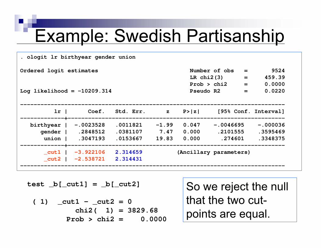
Example: Swedish Partisanship. ologit lr birthyear gender union
Ordered logit estimates Number of obs = 9524LR chi2(3) = 459.39Prob > chi2 = 0.0000
Log likelihood = -10209.314 Pseudo R2 = 0.0220
------------------------------------------------------------------------------lr | Coef. Std. Err. z P>|z| [95% Conf. Interval]
-------------+----------------------------------------------------------------birthyear | -.0023528 .0011821 -1.99 0.047 -.0046695 -.000036
gender | .2848512 .0381107 7.47 0.000 .2101555 .3595469union | .3047193 .0153667 19.83 0.000 .274601 .3348375
-------------+----------------------------------------------------------------_cut1 | -3.922106 2.314659 (Ancillary parameters)_cut2 | -2.538721 2.314431
------------------------------------------------------------------------------
test _b[_cut1] = _b[_cut2]
( 1) _cut1 - _cut2 = 0chi2( 1) = 3829.68
Prob > chi2 = 0.0000
So we reject the null that the two cut-points are equal.


