1300 Henley Court Pullman, WA 99163

509.334.6306 www.store.digilent.com

Lab 7b: Digital Spectrum Analyzer

Revised March 13, 2017 This manual applies to Unit 7, Lab 7b.

Unit 7, Lab 7b Copyright Digilent, Inc. All rights reserved. Other product and company names mentioned may be trademarks of their respective owners. Page 1 of 12

1 Objectives

1. Read analog data from the Basys MX3 microphone.

2. Process a block of analog data with a Discrete Fourier Transform algorithm.

3. Use the Basys MX3 Character LCD to display graphical data.

2 Basic Knowledge

1. Knowledge of C or C++ programming

2. Working knowledge of MPLAB® X IDE

3. How to display text on a character LCD

4. Understanding of Discrete Fourier Transform principles

3 Equipment List

3.1 Hardware

1. Basys MX3 trainer board

2. Workstation computer running Windows 10 or higher, MAC OS, or Linux

3. 2 Standard USB A to micro-B cables

In addition, we suggest the following instruments:

4. Analog Discovery 2

3.2 Software

The following programs must be installed on your development work station:

1. Microchip MPLAB X® v3.35 or higher

2. PLIB Peripheral Library

3. XC32 Cross Compiler

4. WaveForms 2015 (if using the Analog Discovery 2)

Lab 7b: Digital Spectrum Analyzer

Copyright Digilent, Inc. All rights reserved. Other product and company names mentioned may be trademarks of their respective owners. Page 2 of 12

4 Project Takeaways

1. How to implement a fast Fourier transform in C using a PIC32MX microprocessor.

2. How to use the PIC32 processor to analyze a signal in real time.

3. How to display the spectral energy of a real-time signal.

4. How to generate a graphical display on a character LCD.

5 Fundamental Concepts

This unit focuses on processing signals in the audio frequency range using digital signal processing (DSP) concepts

with the PIC32MX370 microprocessor. This lab uses Discrete Fourier Transforms (DFT) to detect the presence of

signals within specified frequency bands. The purpose is to teach how to implement fast Fourier transforms using

the MIPS DSP library function for the PIC32MX microprocessor in lieu of specialized digital signal processors.

5.1 Feedback Control

The Fourier Transform is an essential mathematical tool for studying many natural phenomena and engineering

problems. The Fourier Transform is used to decompose time domain signals, such as the one expressed by Eq. 5.1,

into a combination of sine waves of varying amplitude and phase, as expressed by Eq. 5.2. Note that while Eq. 5.1

expresses x as a function of time, Eq. 5.2 expresses x as a function of frequency, f. Since both x(t) and X(f) are

continuous in nature, they represent expressions that cannot be operated on by a digital computer. Hence x(t)

must first be sampled using an analog-to-digital converter (ADC) that has a constant sampling period, Ts. The

sampling frequency, Fs, is the inverse of the sampling period Ts. This allows the approximation of Eq. 5.2, using a

Discrete Fourier Transform (DFT) algorithm.

𝑥(𝑡) = 𝐴𝑚sin(2𝜋𝑓0𝑡 + 𝜑) Eq. 5.1

𝑋(𝑓) = ∫ 𝑥(𝑡) ∙ 𝑒−𝑗2𝜋𝑡𝑓0𝑑𝑓∞

𝑡=−∞ Eq. 5.2

5.2 Discrete Fourier Transform

When the continuous time domain signal of Eq. 5.1 is sampled, we get a series of discrete data values as a function

of the sample number, as shown in Eq. 5.3. Eq. 5.4 is the expression for converting the series of sampled inputs

into a set of complex values representing the phase and magnitude of the original signal at discrete frequencies.

Since x(n) represents samples of a continuous signal at discrete points in time, Xk represents the same signal as

discrete frequencies, hence the Discrete Fourier Transform or DFT.

There is a one to one correlation of the range of n to the range of k. This means that processing N samples of data

will result in the magnitude and phase of N discrete frequency components, starting with the sampling frequency,

zero and continuing to Fs/2 in steps of Fs/N.

𝑥(𝑛) = 𝐴𝑚 sin(2𝜋𝑓𝑛𝑇 + 𝜑) Eq. 5.3

𝑋𝑘 = ∑ 𝑥𝑛𝑁−1𝑛=0 𝑒−𝑗2𝜋𝑘

𝑛

𝑁 = ∑ 𝑥𝑛 ∙ [cos (2𝜋𝑘𝑛

𝑁) − 𝑗𝑠𝑖𝑛 (

2𝜋𝑘𝑛

𝑁)]𝑁−1

𝑛=0 Eq. 5.4

While Eq. 5.4 is the analysis equation, Eq. 5.5 is the synthesis equation. Note that the only differences between Eq.

5.4 and Eq. 5.5 are the (1/N) multiplier and the sign of the complex exponent of e. A complex signal can be

Lab 7b: Digital Spectrum Analyzer

Copyright Digilent, Inc. All rights reserved. Other product and company names mentioned may be trademarks of their respective owners. Page 3 of 12

represented in the form of the summation of a selected set of complex pairs, or magnitude-phase pairs, that can

be used to reconstruct a very large original time domain signal, thus constituting a form of data compression.

𝑥𝑛 =1

𝑁∑ 𝑋𝑘𝑒

𝑗2𝜋𝑘𝑛

𝑁𝑁−1𝑘=0 Eq. 5.5

Listing A.1 of Appendix A is the C code for implementing the algorithm of Eq. 5.4 in the form of a non-recursive, or

finite impulse response filter (FIR). FIR filters are discussed in some detail in the Unit 7 text. Although the code is

straightforward, the algorithm applied to any large size data set will require extensive computer execution time to

complete the computations. The computational complexity, (based upon the number of multiply and accumulate

or MAC operations) is frequently expressed as the order of N squared, or O(N2), where N is the size of the DFT.

Measurements show that 16.690 ms is required to compute a 32 point DFT when running on the PIC32MX370

processor at 80 MHz. This leads us to the conclusion that it would require four times as long to compute a DFT

twice the size. One can easily see that DFT processing of large data sets can overwhelm a microcontroller with

limited capability.

5.3 Fast Fourier Transform C Code

A fast Fourier transform (FFT) is a discrete Fourier transform algorithm which reduces the number of computations

needed for a size N DFT from 2N2 to 2log(N)2. The caveat is that N must be a power of 2. Although the theory

behind the FFT algorithm is beyond the scope of this tutorial, its application to creating a spectrum analyzer is not.

Using an FFT algorithm reduces the number of MAC instructions from 4096 to 320. Listing A.2 through A.4 are the

functions to implement the Cooley-Tukey FFT algorithm using conventional C statements. The execution time for a

32 point FFT using this algorithm is reduced to 252 μs, which is 66 times faster than the execution speed for the

DFT algorithm shown in Listing A.1. (Wow!)

As the famous infomercials shout, “Wait! That’s not all!” Using the MIPS DSP library mips_ff16 function we can

reduce the execution time to 26 μs. This is almost 10 times faster than the C code in Listings A.2 through A.4 and is

642 times faster than Listing A.1! Is the MIPS DSP library using magic? Not quite. The MIPS DSP library function

shown in Listing A.6 is optimized in assembler language. That’s why it is called a fast Fourier transform.

Listing A.5 declares the coefficient array in the statement, #define fftc fft16c32, which declares an array of 32 16-

bit signed constants that are pre-defined FFT coefficients. In Listing A.6, the line of code mips_fft16( FOut,

TIn, (int16c *)fftc, Scratch, LOG2FFTLEN); shows there are pointers to four arrays and an integer is

passed as arguments. Fout, the result array, and Tin, the input data, are 2 by N 16-bit integer arrays for the real

and imaginary parts of the variable. Although Tin is a complex variable array, the imaginary part is set to zero for

real data sets. The array (int16c *)fftc is defined above. The Scratch array is used for temporary results

that do not need to be remembered from one function call to the next. Finally, the integer, LOG2FFTLEN, is the log

base 2 of the number of points in the FFT.

Since all of the DFT algorithms described in Listing A.1 through return arrays that contain complex values, they

must be converted to real values to be usable for graphical LCD display. Listing 6.7 provides the source code for

converting a pair of complex integer values to a real integer. Tests have shown that the execution time of integer

conversion is three time faster than using a floating point square root function. See Reference 6 for additional

details regarding this algorithm.

The DFT results cover the span of zero to 2π, corresponding to zero to the sampling frequency, Fs. Each output

represents the signal frequency in steps of Fs/N (ΔN) where N is the number of samples being processed. The DFT

output is only valid for the first n = 0 to N/2 – 1 frequencies, or from zero to (Fs/2 – ΔN). The outputs for the n =

N/2 to N-1 frequencies are complex conjugates of the first and can be ignored for our purposes.

Lab 7b: Digital Spectrum Analyzer

Copyright Digilent, Inc. All rights reserved. Other product and company names mentioned may be trademarks of their respective owners. Page 4 of 12

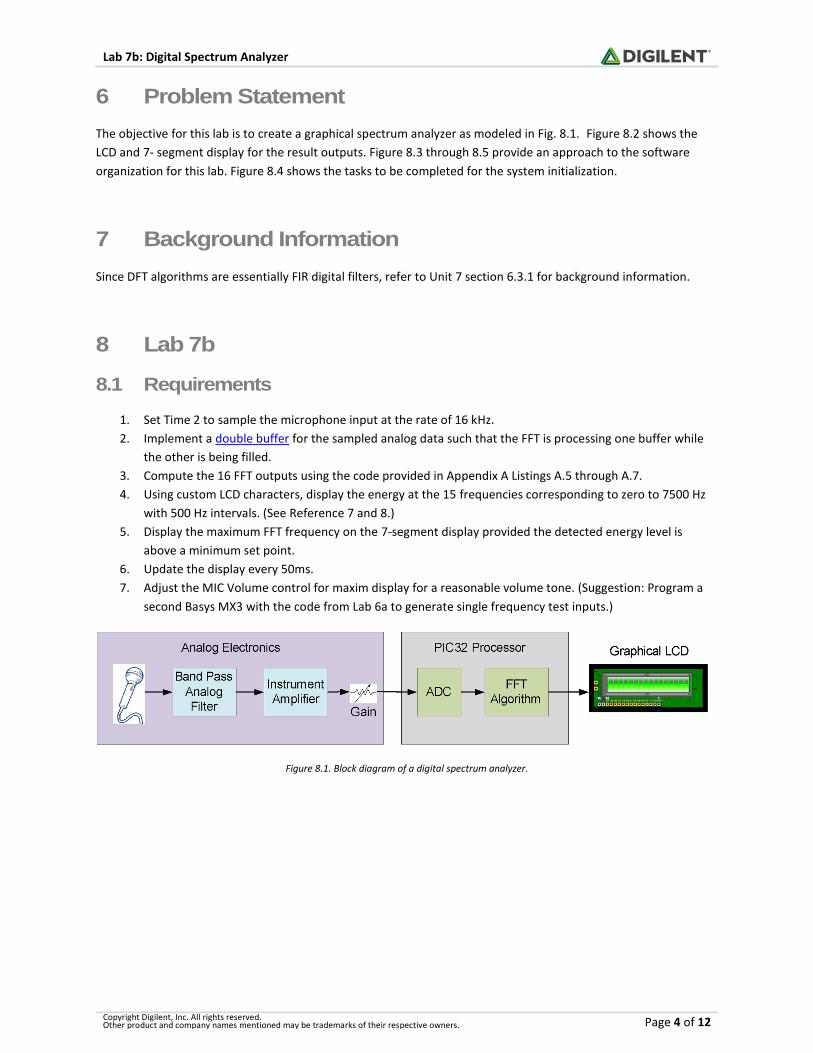
6 Problem Statement

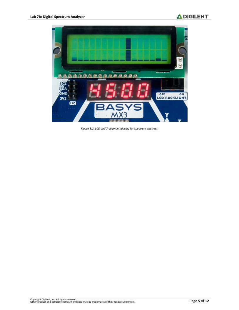
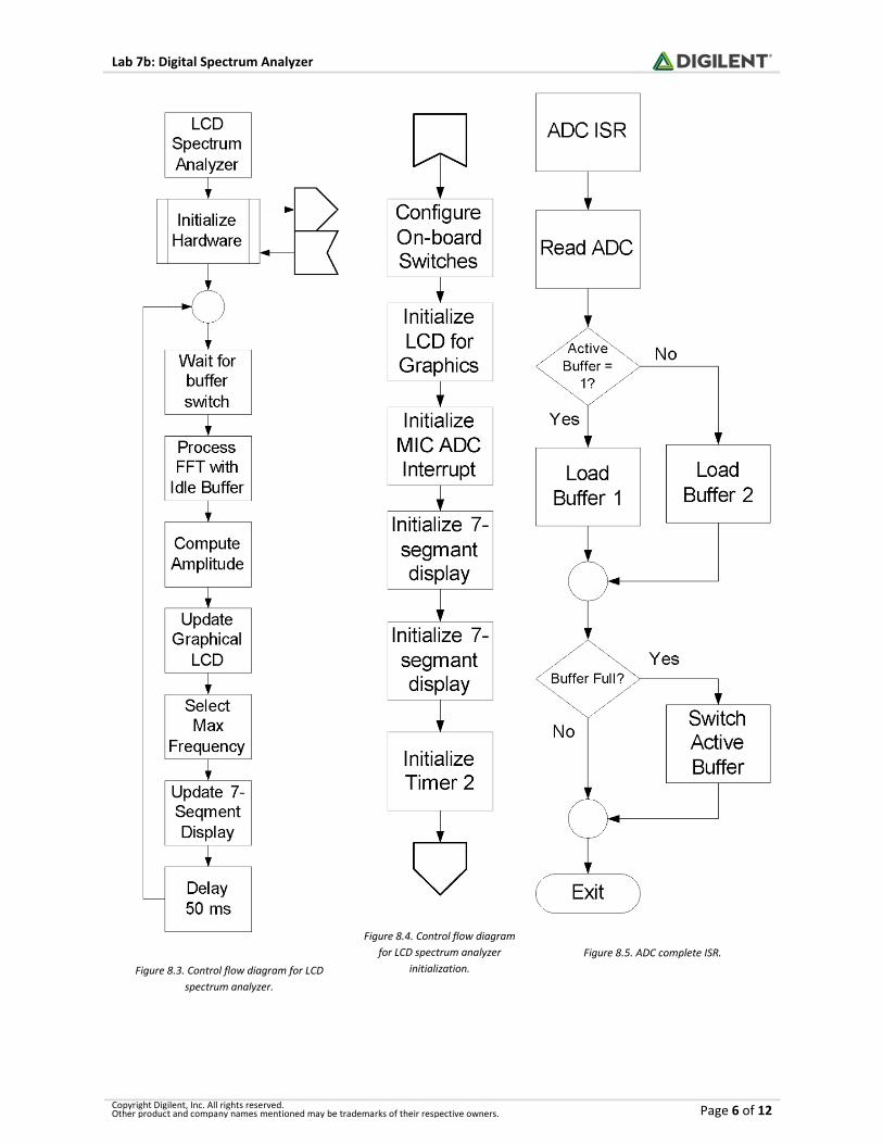
The objective for this lab is to create a graphical spectrum analyzer as modeled in Fig. 8.1. Figure 8.2 shows the

LCD and 7- segment display for the result outputs. Figure 8.3 through 8.5 provide an approach to the software

organization for this lab. Figure 8.4 shows the tasks to be completed for the system initialization.

7 Background Information

Since DFT algorithms are essentially FIR digital filters, refer to Unit 7 section 6.3.1 for background information.

8 Lab 7b

8.1 Requirements

1. Set Time 2 to sample the microphone input at the rate of 16 kHz.

2. Implement a double buffer for the sampled analog data such that the FFT is processing one buffer while

the other is being filled.

3. Compute the 16 FFT outputs using the code provided in Appendix A Listings A.5 through A.7.

4. Using custom LCD characters, display the energy at the 15 frequencies corresponding to zero to 7500 Hz

with 500 Hz intervals. (See Reference 7 and 8.)

5. Display the maximum FFT frequency on the 7-segment display provided the detected energy level is

above a minimum set point.

6. Update the display every 50ms.

7. Adjust the MIC Volume control for maxim display for a reasonable volume tone. (Suggestion: Program a

second Basys MX3 with the code from Lab 6a to generate single frequency test inputs.)

Figure 8.1. Block diagram of a digital spectrum analyzer.

Lab 7b: Digital Spectrum Analyzer

Copyright Digilent, Inc. All rights reserved. Other product and company names mentioned may be trademarks of their respective owners. Page 5 of 12

Figure 8.2. LCD and 7-segment display for spectrum analyzer.

Lab 7b: Digital Spectrum Analyzer

Copyright Digilent, Inc. All rights reserved. Other product and company names mentioned may be trademarks of their respective owners. Page 6 of 12

Figure 8.3. Control flow diagram for LCD

spectrum analyzer.

Figure 8.4. Control flow diagram

for LCD spectrum analyzer

initialization.

Figure 8.5. ADC complete ISR.

Lab 7b: Digital Spectrum Analyzer

Copyright Digilent, Inc. All rights reserved. Other product and company names mentioned may be trademarks of their respective owners. Page 7 of 12

8.2 Design, Construction, Testing

In previous labs, steps were laid out to lead the student through effective design, construction and testing

procedures. This is now left up to the student to complete on their own, ensuring the design requirements listed in

section 8.1 are met.

9 Questions

1. Theoretically, how much time is required to fill one data buffer?

2. Theoretically, what is the maximum rate that the LCD and 7-Segment display can be updated?

3. In reality, what is the maximum rate that the LCD and 7-Segment display can be updated?

4. Why would one want to update the displays at a rate slower than the theoretical maximum speed?

5. How many times will a buffer be filled during the time needed to display the results for computing the FFT

of one block of data? What are the potential problems here?

6. How can your answer to question 5 be resolved?

10 References

1. Basys MX3 Trainer Board Reference Manual.

2. C Programming Reference.

3. PIC32 Family Reference Manual, Timers Section 14:

http://ww1.microchip.com/downloads/en/DeviceDoc/61105E.pdf.

4. Steven W. Smith, The Scientist and Engineer’s Guide to Digital Signal Processing,

http://www.dspguide.com/pdfbook.htm.

5. Cooley-Tukey FFT for 16-bit Integer Numbers, Microchip Technology,

http://www.embeddedcodesource.com/codesnippet/cooley-tukey-fft-for-16-bit-integer-numbers.

6. Calculate an integer square root, http://www.codecodex.com/wiki/Calculate_an_integer_square_root.

7. Printing Custom Characters on a Character LCD, http://deanandara.com/robots/ApuLcd.html.

8. Getting Graphic; Defining Custom LCD Characters, https://www.seetron.com/archive/pdf/lcd_an2.pdf.

Lab 7b: Digital Spectrum Analyzer

Copyright Digilent, Inc. All rights reserved. Other product and company names mentioned may be trademarks of their respective owners. Page 8 of 12

Appendix A: Discrete Fourier Transform Software

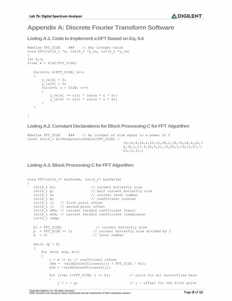
Listing A.1. Code to Implement a DFT Based on Eq. 5.4

#define FFT_SIZE ### // Any integer value void DFT(int16_t *x, int16_t *y_re, int16_t *y_im) { int k,n; float w = PIx2/FFT_SIZE; for(k=0; k<FFT_SIZE; k++) { y_re[k] = 0; y_im[k] = 0; for(n=0; n < SIZE; n++) { y_re[k] += x[n] * cos(w * n * k); y_im[k] += x[n] * sin(w * n * k); } } }

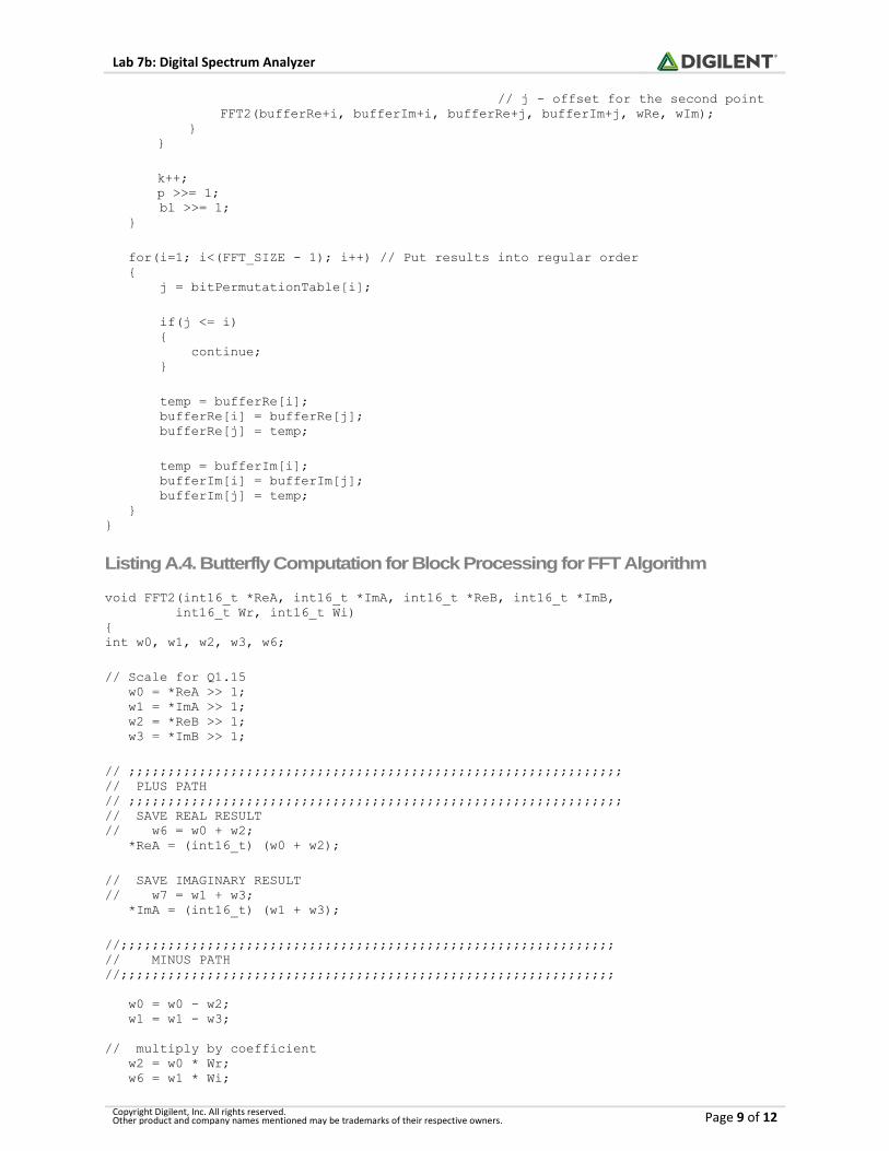
Listing A.2. Constant Declarations for Block Processing C for FFT Algorithm

#define FFT_SIZE ### // An integer of size equal to a power of 2 const int16_t bitPermutationTable[FFT_SIZE] =

{0,16,8,24,4,20,12,28,2,18,10,26,6,22,1 4,30,1,17,9,25,5,21,13,29,3,19,11,27,7, 23,15,31};

Listing A.3. Block Processing C for FFT Algorithm

void FFT(int16_t* bufferRe, int16_t* bufferIm) { int16_t bl; // current butterfly size int16_t p; // half current butterfly size int16_t k; // current level number int16_t m; // coefficient counter int16_t i; // first point offset int16_t j; // second point offset int16_t wRe; // current twiddle coefficient (real) int16_t wIm; // current twiddle coefficient (imaginary) int16_t temp; bl = FFT_SIZE; // current butterfly size p = FFT_SIZE >> 1; // current butterfly size divided by 2 k = 0; // level number while (p > 0) { for (m=0; m<p; m++) { j = m << k; // coefficient offset wRe = twiddleCoefficients[(j + FFT_SIZE / 4)]; wIm = -twiddleCoefficients[j]; for (i=m; i<FFT_SIZE; I += bl) // cycle for all butterflies here { j = i + p; // i - offset for the first point

Lab 7b: Digital Spectrum Analyzer

Copyright Digilent, Inc. All rights reserved. Other product and company names mentioned may be trademarks of their respective owners. Page 9 of 12

// j - offset for the second point FFT2(bufferRe+i, bufferIm+i, bufferRe+j, bufferIm+j, wRe, wIm);

} } k++; p >>= 1; bl >>= 1; } for(i=1; i<(FFT_SIZE - 1); i++) // Put results into regular order { j = bitPermutationTable[i]; if(j <= i) { continue; } temp = bufferRe[i]; bufferRe[i] = bufferRe[j]; bufferRe[j] = temp; temp = bufferIm[i]; bufferIm[i] = bufferIm[j]; bufferIm[j] = temp; } }

Listing A.4. Butterfly Computation for Block Processing for FFT Algorithm

void FFT2(int16_t *ReA, int16_t *ImA, int16_t *ReB, int16_t *ImB, int16_t Wr, int16_t Wi) { int w0, w1, w2, w3, w6; // Scale for Q1.15 w0 = *ReA >> 1; w1 = *ImA >> 1; w2 = *ReB >> 1; w3 = *ImB >> 1; // ;;;;;;;;;;;;;;;;;;;;;;;;;;;;;;;;;;;;;;;;;;;;;;;;;;;;;;;;;;;;;;; // PLUS PATH // ;;;;;;;;;;;;;;;;;;;;;;;;;;;;;;;;;;;;;;;;;;;;;;;;;;;;;;;;;;;;;;; // SAVE REAL RESULT // w6 = w0 + w2; *ReA = (int16_t) (w0 + w2); // SAVE IMAGINARY RESULT // w7 = w1 + w3; *ImA = (int16_t) (w1 + w3); //;;;;;;;;;;;;;;;;;;;;;;;;;;;;;;;;;;;;;;;;;;;;;;;;;;;;;;;;;;;;;;; // MINUS PATH //;;;;;;;;;;;;;;;;;;;;;;;;;;;;;;;;;;;;;;;;;;;;;;;;;;;;;;;;;;;;;;; w0 = w0 - w2; w1 = w1 - w3; // multiply by coefficient w2 = w0 * Wr; w6 = w1 * Wi;

Lab 7b: Digital Spectrum Analyzer

Copyright Digilent, Inc. All rights reserved. Other product and company names mentioned may be trademarks of their respective owners. Page 10 of 12

w2 = (w2 - w6) >> 15; // SAVE RESULT W3 HERE (REAL) // w2 = w2 >> 15; *ReB = (int16_t) w2 ; // multiply by coefficient w2 = w0 * Wi; w6 = w1 * Wr; w2 = (w2 + w6) >> 15; // SAVE RESULT W3 HERE (IMAGINARY) *ImB = (int16_t) w2; }

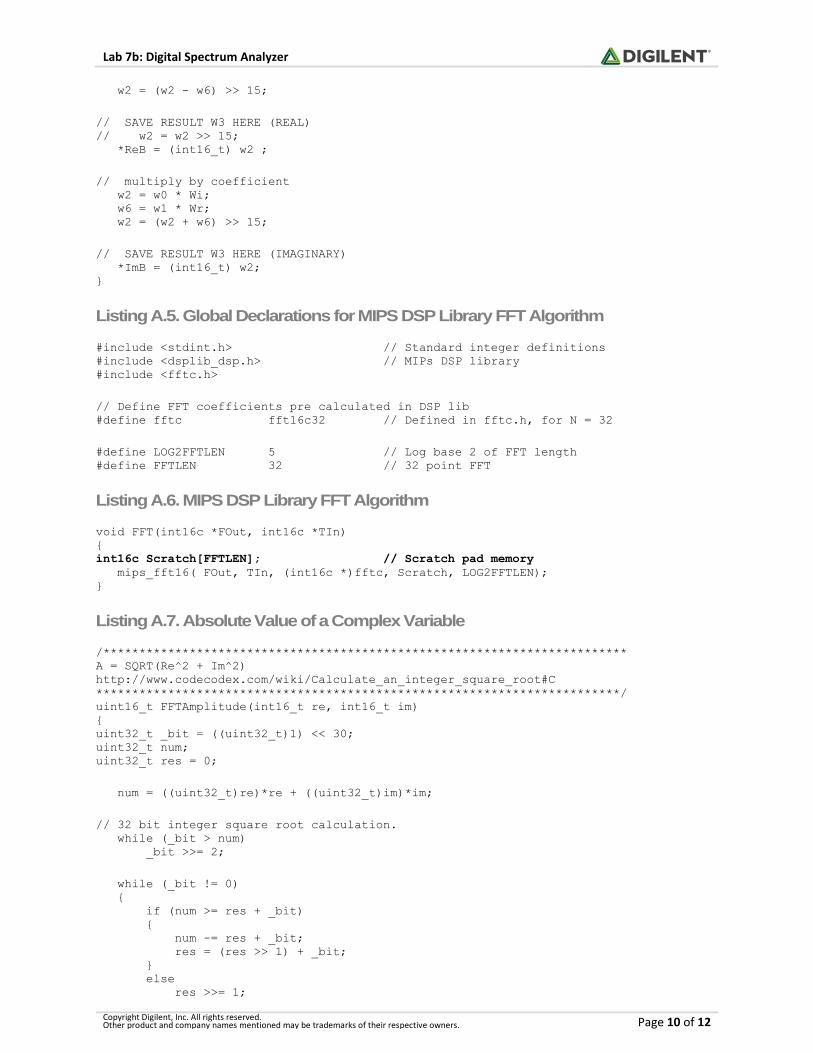
Listing A.5. Global Declarations for MIPS DSP Library FFT Algorithm

#include <stdint.h> // Standard integer definitions #include <dsplib_dsp.h> // MIPs DSP library #include <fftc.h> // Define FFT coefficients pre calculated in DSP lib #define fftc fft16c32 // Defined in fftc.h, for N = 32 #define LOG2FFTLEN 5 // Log base 2 of FFT length #define FFTLEN 32 // 32 point FFT

Listing A.6. MIPS DSP Library FFT Algorithm

void FFT(int16c *FOut, int16c *TIn) { int16c Scratch[FFTLEN]; // Scratch pad memory mips_fft16( FOut, TIn, (int16c *)fftc, Scratch, LOG2FFTLEN); }

Listing A.7. Absolute Value of a Complex Variable

/************************************************************************* A = SQRT(Re^2 + Im^2) http://www.codecodex.com/wiki/Calculate_an_integer_square_root#C *************************************************************************/ uint16_t FFTAmplitude(int16_t re, int16_t im) { uint32_t _bit = ((uint32_t)1) << 30; uint32_t num; uint32_t res = 0; num = ((uint32_t)re)*re + ((uint32_t)im)*im; // 32 bit integer square root calculation. while (_bit > num) _bit >>= 2; while (_bit != 0) { if (num >= res + _bit) { num -= res + _bit; res = (res >> 1) + _bit; } else res >>= 1;

Lab 7b: Digital Spectrum Analyzer

Copyright Digilent, Inc. All rights reserved. Other product and company names mentioned may be trademarks of their respective owners. Page 11 of 12

_bit >>= 2; } return ((uint16_t)res); }

Lab 7b: Digital Spectrum Analyzer

Copyright Digilent, Inc. All rights reserved. Other product and company names mentioned may be trademarks of their respective owners. Page 12 of 12

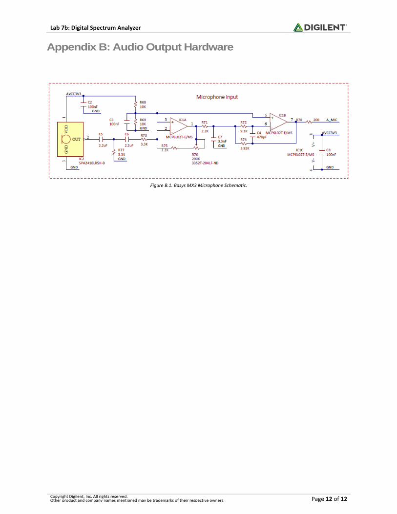
Appendix B: Audio Output Hardware

Figure B.1. Basys MX3 Microphone Schematic.