Download - Kernel Logistic Regression and the Import Vector …dept.stat.lsa.umich.edu/~jizhu/pubs/Zhu-JCGS05.pdf · Kernel Logistic Regression and the Import Vector Machine ... Recently Keerthi,

Kernel Logistic Regression and the ImportVector Machine

Ji ZHU and Trevor HASTIE

The support vector machine (SVM) is known for its good performance in two-classclassification, but its extension to multiclass classification is still an ongoing research is-sue. In this article, we propose a new approach for classification, called the import vectormachine (IVM), which is built on kernel logistic regression (KLR). We show that the IVMnot only performs as well as the SVM in two-class classification, but also can naturallybe generalized to the multiclass case. Furthermore, the IVM provides an estimate of theunderlying probability. Similar to the support points of the SVM, the IVM model uses onlya fraction of the training data to index kernel basis functions, typically a much smallerfraction than the SVM. This gives the IVM a potential computational advantage over theSVM.

Key Words: Classification; Kernel methods; Multiclass learning; Radial basis; Reproduc-ing kernel Hilbert space (RKHS); Support vector machines.

1. INTRODUCTION

In standard classification problems, we are given a set of training data (x1, y1), (x2, y2),. . . , (xn, yn), where the input xi ∈ Rp and the output yi is qualitative and assumes valuesin a finite set C, for example, C = {1, 2, . . . , C}. We wish to find a classification rule fromthe training data, so that when given a new input x, we can assign a class c from C to it.Usually it is assumed that the training data are an independently and identically distributedsample from an unknown probability distribution P (X,Y ).

The support vector machine (SVM) works well in two-class classification, that is,y ∈ {−1, 1}, but its appropriate extension to the multiclass case is still an ongoing researchissue (e.g., Vapnik 1998; Weston and Watkins 1999; Bredensteiner and Bennett 1999; Lee,Lin, and Wahba 2002). Another property of the SVM is that it only estimates sign[p(x)−1/2]

Ji Zhu is Assistant Professor, Department of Statistics, University of Michigan, Ann Arbor, MI 48109-1092 (E-mail: [email protected]). Trevor Hastie is Professor, Department of Statistics, Stanford University, Stanford, CA94305 (E-mail: [email protected]).

c©2005 American Statistical Association, Institute of Mathematical Statistics,and Interface Foundation of North America

Journal of Computational and Graphical Statistics, Volume 14, Number 1, Pages 185–205DOI: 10.1198/106186005X25619

185

186 J. ZHU AND T. HASTIE

(Lin 2002), while the probability p(x) is often of interest itself, where p(x) = P (Y =1|X = x) is the conditional probability of a point being in class 1 given X = x. In thisarticle, we propose a new approach, called the import vector machine (IVM), to address theclassification problem. We show that the IVM not only performs as well as the SVM in two-class classification, but also can naturally be generalized to the multiclass case. Furthermore,the IVM provides an estimate of the probability p(x). Similar to the support points of theSVM, the IVM model uses only a fraction of the training data to index the kernel basisfunctions. We call these training data import points. The computational cost of the SVM isO(n2ns) (e.g., Kaufman 1999), where ns is the number of support points and ns usuallyincreases linearly with n, while the computational cost of the IVM is O(n2m2), where m

is the number of import points. Because m does not tend to increase as n increases, theIVM can be faster than the SVM. Empirical results show that the number of import pointsis usually much less than the number of support points.

In Section 2, we briefly review some results of the SVM for two-class classificationand compare it with kernel logistic regression (KLR). In Section 3, we propose our IVMalgorithm. In Section 4, we show some numerical results. In Section 5, we generalize theIVM to the multiclass case.

2. SUPPORT VECTOR MACHINES AND KERNEL LOGISTICREGRESSION

The standard SVM produces a nonlinear classification boundary in the original inputspace by constructing a linear boundary in a transformed version of the original input space.The dimension of the transformed space can be very large, even infinite in some cases.This seemingly prohibitive computation is achieved through a positive definite reproducingkernel K(·, ·), which gives the inner product in the transformed space.

Many people have noted the relationship between the SVM and regularized functionestimation in the reproducing kernel Hilbert spaces (RKHS). An overview can be found inBurges (1998), Evgeniou, Pontil, and Poggio (1999), Wahba (1999), and Hastie, Tibshirani,and Friedman (2001). Fitting an SVM is equivalent to

minf∈HK

1n

n∑i=1

[1 − yif(xi)

]+ +

λ

2‖f‖2

HK, (2.1)

where HK is the RKHS generated by the kernel K(·, ·). The classification rule is given bysign[f(x)]. For the purpose of simple notation, we omit the constant term in f(x).

By the representer theorem (Kimeldorf and Wahba 1971), the optimal f(x) has theform:

f(x) =n∑

i=1

aiK(x,xi). (2.2)

It often happens that a sizeable fraction of the n values of ai can be zero. This is a con-sequence of the truncation property of the first part of criterion (2.1). This seems to be an

KERNEL LOGISTIC REGRESSION 187

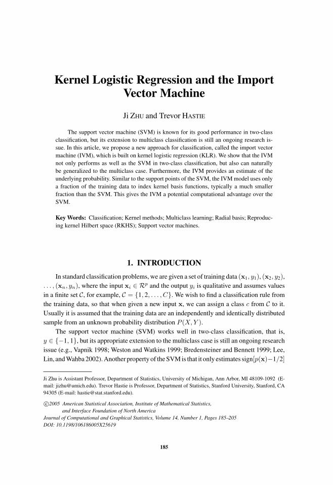
Figure 1. Two loss functions, y ∈ { −1, 1}.

attractive property, because only the points on the wrong side of the classification bound-ary, and those on the right side but near the boundary have an influence in determining theposition of the boundary, and hence have nonzero ai’s. The corresponding xi’s are calledsupport points.

Notice that (2.1) has the form loss + penalty. The loss function (1 − yf)+ is plotted inFigure 1, along with the negative log-likelihood (NLL) of the binomial distribution. As wecan see, the NLL of the binomial distribution has a similar shape to that of the SVM: bothincrease linearly as yf gets very small (negative) and both encourage y and f to have thesame sign. If we replace (1 − yf)+ in (2.1) with ln(1 + e−yf ), the NLL of the binomialdistribution, the problem becomes a kernel logistic regression (KLR) problem:

minf∈HK

1n

n∑i=1

ln(

1 + e−yif(xi))

+λ

2‖f‖2

HK. (2.3)

Because of the similarity between the two loss functions, we expect that the fitted functionperforms similarly to the SVM for two-class classification.

There are two immediate advantages of making such a replacement: (a) Besides givinga classification rule, KLR also offers a natural estimate of the probability p(x) = ef(x)/(1+ef(x)), while the SVM only estimates sign[p(x)−1/2] (Lin 2002); (b) KLR can naturally begeneralized to the multiclass case through kernel multi-logit regression. However, becauseKLR compromises the hinge loss function of the SVM, it no longer has the support pointsproperty; in other words, all the ai’s in (2.2) are nonzero.

KLR is a well-studied problem; see Green and Yandell (1985), Hastie and Tibshirani


(1990), Wahba, Gu, Wang, and Chappell (1995) and the references therein; however, theyare all under the smoothing spline analysis of variance scheme.

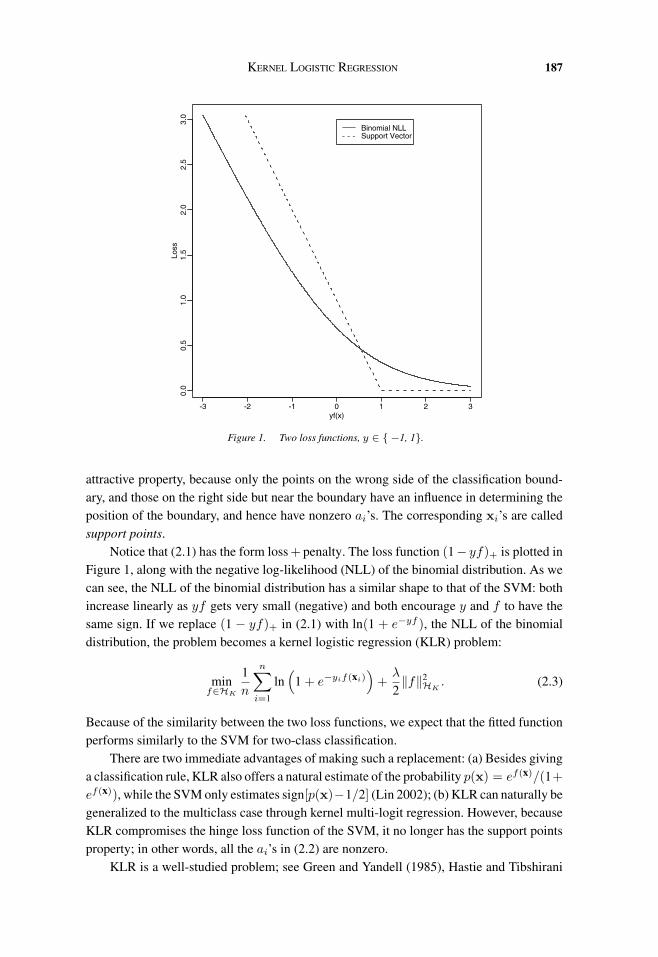
We use a simulation example to illustrate the similar performances between KLR andthe SVM. The data in each class are simulated from a mixture of Gaussian distribution(Hastie et al. 2001): first we generate 10 means µk from a bivariate Gaussian distributionN((1, 0)T , I) and label this class +1. Similarly, 10 more are drawn from N((0, 1)T , I)and labeled class −1. Then for each class, we generate 100 observations as follows: foreach observation, we pick an µk at random with probability 1/10, and then generate aN(µk, I/5), thus leading to a mixture of Gaussian clusters for each class.

We use the radial basis kernel

K(xi,xi′) = e− ‖xi−xi′ ‖2

2σ2 . (2.4)

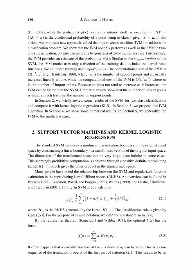
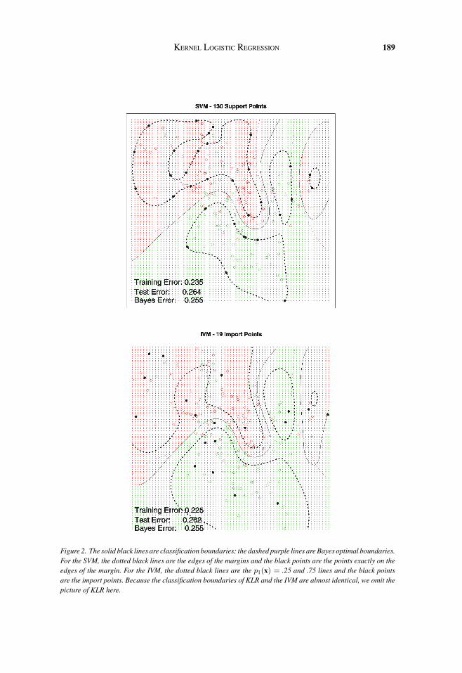
The regularization parameter λ is chosen to achieve good misclassification error. The resultsare shown in Figure 2. The radial basis kernel produces a boundary quite close to the Bayesoptimal boundary for this simulation. We see that the fitted model of KLR is quite similar inclassification performance to that of the SVM. In addition to a classification boundary, sinceKLR estimates the log-odds of class probabilities, it can also produce probability contours(Figure 2).

2.1 KLR AS A MARGIN MAXIMIZER

The SVM was initiated as a method to maximize the margin, that is, mini yif(xi),of the training data; KLR is motivated by the similarity in shape between the NLL of thebinomial distribution and the hinge loss of the SVM. Then a natural question is: what doesKLR do with the margin?

Suppose the dictionary of the basis functions of the transformed feature space is

{h1(x), h2(x), . . . , hq(x)} ,

where q is the dimension of the transformed feature space. Note if q = p and hj(x) is thejth component of x, the transformed feature space is reduced to the original input space.The classification boundary, a hyperplane in the transformed feature space, is given by

{x : f(x) = β0 + h(x)T β = 0}.

Suppose the transformed feature space is so rich that the training data are separable, thenthe margin-maximizing SVM can be written as:

maxβ0,βββ,‖βββ‖2=1

D (2.5)

subject to yi

(β0 + h(xi)T β

) ≥ D, i = 1, . . . , n (2.6)

where D is the shortest distance from the training data to the separating hyperplane and isdefined as the margin (Burges 1998).


Figure 2. The solid black lines are classification boundaries; the dashed purple lines are Bayes optimal boundaries.For the SVM, the dotted black lines are the edges of the margins and the black points are the points exactly on theedges of the margin. For the IVM, the dotted black lines are the p1(x) = .25 and .75 lines and the black pointsare the import points. Because the classification boundaries of KLR and the IVM are almost identical, we omit thepicture of KLR here.


Now consider an equivalent setup of KLR:

minβ0,βββ

n∑i=1

ln(

1 + e−yif(xi))

(2.7)

subject to ‖β‖22 ≤ s (2.8)

f(xi) = β0 + h(xi)T β, i = 1, . . . , n. (2.9)

Then we have Theorem 1.

Theorem 1. Suppose the training data are separable, that is, ∃β0,β, s.t. yi(β0 +h(xi)T β) > 0, ∀i. Let the solution of (2.7)–(2.9) be denoted by β(s), then

β(s)s

→ β∗ as s → ∞,

where β∗ is the solution of the margin-maximizing SVM (2.5)–(2.6), if β∗ is unique.

If β∗ is not unique, then βββ(s)s may have multiple convergence points, but they will all

represent margin-maximizing separating hyperplanes.

The proof of the theorem appears in the Appendix. Theorem 1 implies that KLR, similarto the SVM, can also be considered as a margin maximizer. We have also proved a moregeneral theorem relating loss functions and margin maximizers in Rosset, Zhu, and Hastie(2004).

2.2 COMPUTATIONAL CONSIDERATIONS

Because (2.3) is convex, it is natural to use the Newton-Raphson method to fit KLR. Inorder to guarantee convergence, suitable bisection steps can be combined with the Newton-Raphson iterations. The drawback of the Newton-Raphson method is that in each iteration,an n × n matrix needs to be inverted. Therefore the computational cost of KLR is O(n3).Recently Keerthi, Duan, Shevade, and Poo (2002) proposed a dual algorithm for KLRwhich avoids inverting huge matrices. It follows the spirit of the popular sequential minimaloptimization (SMO) algorithm (Platt 1999). Preliminary computational experiments showthat the algorithm is robust and fast. Keerthi et al. (2002) described the algorithm for two-class classification; we have generalized it to the multiclass case (Zhu and Hastie 2004).

Although the sequential minimal optimization method helps reduce the computationalcost of KLR, in the fitted model (2.2), all the ai’s are nonzero. Hence, unlike the SVM,KLR does not allow for data compression and does not have the advantage of less storageand quicker evaluation.

In this article, we propose an import vector machine (IVM) model that finds a submodelto approximate the full model (2.2) given by KLR. The submodel has the form:

f(x) =∑xi∈S

aiK(x,xi), (2.10)

where S is a subset of the training data {x1,x2, . . . ,xn}, and the data in S are called importpoints. The advantage of this submodel is that the computational cost is reduced, especially


for large training datasets, while not jeopardizing the performance in classification; andsince only a subset of the training data are used to index the fitted model, data compressionis achieved.

Several other researchers have also investigated techniques in selecting the subset S.Lin et al. (2000) divided the training data into several clusters, then randomly selected arepresentative from each cluster to make up S. Smola and Scholkopf (2000) developed agreedy technique to sequentially select m columns of the kernel matrix [K(xi,xi′)]n×n,such that the span of these m columns approximates the span of [K(xi,xi′)]n×n well inthe Frobenius norm. Williams and Seeger (2001) proposed randomly selecting m points ofthe training data, then using the Nystrom method to approximate the eigen-decompositionof the kernel matrix [K(xi,xi′)]n×n, and expanding the results back up to n dimensions.None of these methods uses the output yi in selecting the subset S (i.e., the procedure onlyinvolves xi). The IVM algorithm uses both the output yi and the input xi to select the subsetS, in such a way that the resulting fit approximates the full model well. The idea is similarto that used in Luo and Wahba (1997), which also used the output yi to select a subset ofthe training data, but under the regression scheme.

3. IMPORT VECTOR MACHINES

In KLR, we want to minimize

H =1n

n∑i=1

ln(

1 + e−yif(xi))

+λ

2‖f‖2

HK. (3.1)

Let

pi =1

1 + e−yif(xi), i = 1, . . . n (3.2)

a = (a1, . . . , an)T (3.3)

p = (p1, . . . , pn)T (3.4)

y = (y1, . . . , yn)T (3.5)

K1 =(K(xi,xi′)

)n

i,i′=1(3.6)

K2 = K1 (3.7)

W = diag(p1(1 − p1), . . . , pn(1 − pn)

). (3.8)

With some abuse of notation, using (2.2), (3.1) can be written in a finite dimensional form:

H =1n1T ln

(1 + e−y·(K1a)

)+

λ

2aT K2a, (3.9)

where “·” denotes element-wise multiplication. To find a, we set the derivative of H withrespect to a equal to 0, and use the Newton-Raphson method to iteratively solve the scoreequation. It can be shown that the Newton-Raphson step is a weighted least squares step:

a(k) =(

1nKT

1 WK1 + λK2

)−1

KT1 Wz, (3.10)


where a(k) is the value of a in the kth step, and

z =1n

(K1a(k−1) + W−1(y · p)

). (3.11)

3.1 BASIC ALGORITHM

As mentioned in Section 2, we want to find a subset S of {x1,x2, . . . ,xn}, such that thesubmodel (2.10) is a good approximation of the full model (2.2). Because searching for everysubset S is a combinatorial problem and computationally prohibitive, we use the followinggreedy forward strategy: we start with the null model, that is, S = ∅, then iteratively buildup S one element at a time. Basically, we look for a data point among {x1,x2, . . . ,xn}\S,so that if it is added into the current S, the new submodel will decrease the regularizednegative log-likelihood the most:

Algorithm 1: Basic IVM Algorithm.1. Let S = ∅, L = {x1,x2, . . . ,xn}, k = 1.2. For each xl ∈ L, let

fl(x) =∑

xi∈S∪{xl}aiK(x,xi).

Use the Newton-Raphson method to find a to minimize

H(xl) =1n

n∑i=1

ln(1 + exp(−yifl(xi))

)+

λ

2‖fl(x)‖2

HK(3.12)

=1n1T ln

(1 + exp(−y · (Kl

1a)))

+λ

2aT Kl

2a, (3.13)

where the regressor matrix

Kl1 =

(K(xi,xi′)

)n×k

, xi ∈ {x1, . . . ,xn},xi′ ∈ S ∪ {xl};

the regularization matrix

Kl2 =

(K(xi,xi′)

)k×k

,xi,xi′ ∈ S ∪ {xl};

and k = |S| + 1.3. Find

xl∗ = argminxl∈L

H(xl).

Let S = S ∪ {xl∗}, L = L \ {xl∗}, Hk = H(xl∗), k = k + 1.4. Repeat Steps 2 and 3 until Hk converges.

The points in S are the import points.


3.2 REVISED ALGORITHM

The above algorithm is computationally feasible, but in Step 2 we need to use theNewton-Raphson method to find a iteratively. When the number of import points k becomeslarge, the Newton-Raphson computation can be expensive. To reduce this computation, weuse a further approximation.

Instead of iteratively computing a(k) until it converges, we can just do a one-stepiteration, and use it as an approximation to the converged one. This is equivalent to ap-proximating the negative binomial log-likelihood with a different weighted quadratic lossfunction at each iteration. To get a good approximation, we take advantage of the fittedresult from the current “optimal” S, that is, the submodel when |S| = k − 1, and use it tocompute z in (3.11). This one-step update is similar to the score test in generalized linearmodels (GLM); but the latter does not have a penalty term. The updating formula allowsthe weighted regression (3.10) to be computed in O(nm) time.

Hence, we have the revised Steps 1 and 2 for the basic algorithm:

Algorithm 2: Revised Steps 1 and 2.1∗ Let S = ∅, L = {x1,x2, . . . ,xn}, k = 1. Let a(0) = 0, hence z = 2y/n.2∗ For each xl ∈ L, correspondingly augment K1 with a column, and K2 with a

column and a row. Use the current submodel from iteration (k − 1) to compute z in(3.11) and use the updating formula (3.10) to find a. Compute (3.13).

3.3 STOPPING RULE FOR ADDING POINT TO SIn Step 4 of the basic algorithm, we need to decide whether Hk has converged. A

natural stopping rule is to look at the regularized NLL. Let H1, H2, . . . be the sequence ofregularized NLL’s obtained in Step 3. At each step k, we compare Hk with Hk−∆k, where∆k is a prechosen small integer, for example ∆k = 1. If the ratio |Hk−Hk−∆k|

|Hk| is less thansome prechosen small number ε, for example, ε = .001, we stop adding new import pointsto S.

3.4 CHOOSING THE REGULARIZATION PARAMETER λ

So far, we have assumed that the regularization parameter λ is fixed. In practice, wealso need to choose an “optimal” λ. We can randomly split all the data into a training setand a tuning set, and use the misclassification error on the tuning set as a criterion forchoosing λ. To reduce the computation, we take advantage of the fact that the regularizedNLL converges faster for a larger λ. Thus, instead of running the entire revised algorithmfor each λ, we propose the following procedure, which combines both adding import pointsto S and choosing the optimal λ.

Algorithm 3: Simultaneous Selection of S and λ.1. Start with a large regularization parameter λ.


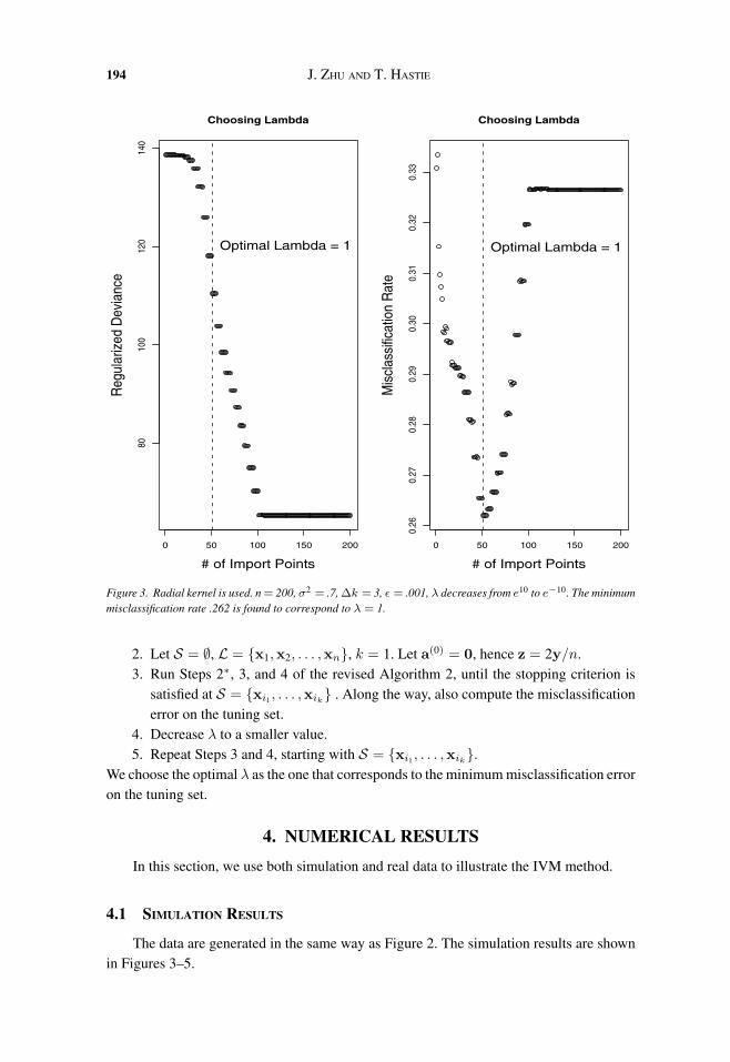
Figure 3. Radial kernel is used. n = 200, σ2 = .7, ∆k = 3, ε = .001, λ decreases from e10 to e−10. The minimummisclassification rate .262 is found to correspond to λ = 1.

2. Let S = ∅, L = {x1,x2, . . . ,xn}, k = 1. Let a(0) = 0, hence z = 2y/n.3. Run Steps 2∗, 3, and 4 of the revised Algorithm 2, until the stopping criterion is

satisfied at S = {xi1 , . . . ,xik} . Along the way, also compute the misclassification

error on the tuning set.4. Decrease λ to a smaller value.5. Repeat Steps 3 and 4, starting with S = {xi1 , . . . ,xik

}.We choose the optimal λ as the one that corresponds to the minimum misclassification erroron the tuning set.

4. NUMERICAL RESULTS

In this section, we use both simulation and real data to illustrate the IVM method.

4.1 SIMULATION RESULTS

The data are generated in the same way as Figure 2. The simulation results are shownin Figures 3–5.


Figure 4. Radial kernel is used. n = 200, σ2 = .7, ∆k = 3, ε = .001, λ = 1. The stopping criterion is satisfiedwhen |S| = 19.

Figure 3 shows how the tuning parameter λ is selected. The optimal λ is found tobe equal to 1 and corresponds to a misclassification rate .262. Figure 4 fixes the tuningparameter to λ = 1 and finds 19 import points. Figure 2 compares the results of the SVMand the IVM: the SVM has 130 support points, and the IVM uses 19 import points; theygive similar classification boundaries. Figure 5 is for the same simulation but different sizesof training data: n = 200, 400, 600, 800. We see that as the size of training data n increases,the number of import points does not tend to increase.

Remarks. The support points of the SVM are those which are close to the classificationboundary or misclassified and usually have large weights p(x)(1−p(x)). The import pointsof the IVM are those that decrease the regularized NLL the most, and can be either closeto or far from the classification boundary. This difference is natural, because the SVM isconcerned only with the classification sign

[p(x) − 1/2

], while the IVM also focuses on

the unknown probability p(x). Though points away from the classification boundary do notcontribute to determining the position of the classification boundary, they may contributeto estimating the unknown probability p(x). The total computational cost of the SVM


Figure 5. The data are generated in the same way as Figures 2–4. Radial kernel is used. σ2 = .7, λ = 1, ∆k = 3,ε = .001. The sizes of training data are n = 200, 400, 600, 800, and the corresponding numbers of import pointsare 19, 18, 19, 18.

is O(n2ns) (e.g., Kaufman 1999), where ns is the number of support points, while thecomputational cost of the IVM method is O(n2m2), where m is the number of importpoints. Since m does not tend to increase as n increases, as illustrated in Figure 5, thecomputational cost of the IVM can be smaller than that of the SVM.

4.2 REAL DATA RESULTS

In this section, we compare the performances of the IVM and the SVM on some realdatasets. Ten benchmark datasets are used for this purpose: Banana, Breast-cancer, Flare-solar, German, Heart, Image, Ringnorm, Splice, Thyroid, Titanic, Twonorm and Waveform.Detailed information about these datasets can be found in Ratsch, Onoda, and Muller (2000).

Table 1 contains a summary of these datasets. Radial kernel (2.4) is used throughoutthese datasets. The parameters σ and λ are fixed at specific values that are optimal for theSVMs generalization performance (Ratsch et al. 2000). Each dataset has 20 realizations ofthe training and test data. The results are in Table 2 and Table 3. The number outside eachbracket is the mean over 20 realizations of the training and test data, and the number ineach bracket is the standard error. From Table 2, we can see that the IVM performs as wellas the SVM in classification on these benchmark datasets. From Table 3, we can see that


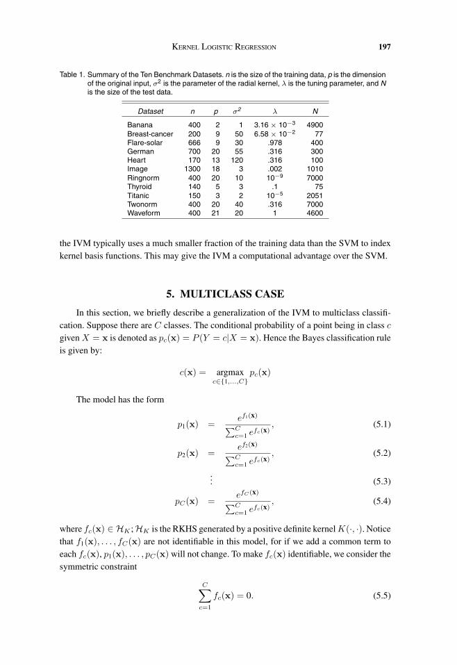
Table 1. Summary of the Ten Benchmark Datasets. n is the size of the training data, p is the dimensionof the original input, σ2 is the parameter of the radial kernel, λ is the tuning parameter, and Nis the size of the test data.

Dataset n p σ2 λ N

Banana 400 2 1 3.16 × 10−3 4900Breast-cancer 200 9 50 6.58 × 10−2 77Flare-solar 666 9 30 .978 400German 700 20 55 .316 300Heart 170 13 120 .316 100Image 1300 18 3 .002 1010Ringnorm 400 20 10 10−9 7000Thyroid 140 5 3 .1 75Titanic 150 3 2 10−5 2051Twonorm 400 20 40 .316 7000Waveform 400 21 20 1 4600

the IVM typically uses a much smaller fraction of the training data than the SVM to indexkernel basis functions. This may give the IVM a computational advantage over the SVM.

5. MULTICLASS CASE

In this section, we briefly describe a generalization of the IVM to multiclass classifi-cation. Suppose there are C classes. The conditional probability of a point being in class c

given X = x is denoted as pc(x) = P (Y = c|X = x). Hence the Bayes classification ruleis given by:

c(x) = argmaxc∈{1,...,C}

pc(x)

The model has the form

p1(x) =ef1(x)∑C

c=1 efc(x)

, (5.1)

p2(x) =ef2(x)∑C

c=1 efc(x)

, (5.2)

... (5.3)

pC(x) =efC(x)∑Cc=1 e

fc(x), (5.4)

where fc(x) ∈ HK ; HK is the RKHS generated by a positive definite kernel K(·, ·). Noticethat f1(x), . . . , fC(x) are not identifiable in this model, for if we add a common term toeach fc(x), p1(x), . . . , pC(x) will not change. To make fc(x) identifiable, we consider thesymmetric constraint

C∑c=1

fc(x) = 0. (5.5)


Table 2. Comparison of Classification Performance of SVM and IVM on Ten Benchmark Datasets

Dataset SVM Error (%) IVM Error (%)

Banana 10.78 (± .68) 10.34 (± .46)Breast-cancer 25.58 (± 4.50) 25.92 (± 4.79)Flare-solar 32.65 (± 1.42) 33.66 (± 1.64)German 22.88 (± 2.28) 23.53 (± 2.48)Heart 15.95 (± 3.14) 15.80 (± 3.49)Image 3.34 (.70) 3.31 (± .80)Ringnorm 2.03 (± .19) 1.97 (± .29)Thyroid 4.80 (± 2.98) 5.00 (± 3.02)Titanic 22.16 (± .60) 22.39 (± 1.03)Twonorm 2.90 (± .25) 2.45 (± .15)Waveform 9.98 (± .43) 10.13 (± .47)

Then the multiclass KLR fits a model to minimize the regularized negative log-likelihood

H = − 1n

n∑i=1

ln pyi(xi) +λ

2‖f‖2

HK(5.6)

=1n

n∑i=1

[−yT

i f(xi) + ln(ef1(xi) + · · · + efC(xi)

)]+

λ

2‖f‖2

HK, (5.7)

where yi is a binary C-vector with values all zero except a 1 in position c if the class is c,and

f(xi) =(f1(xi), . . . , fC(xi)

)T, (5.8)

‖f‖2HK

=C∑

c=1

‖fc‖2HK

. (5.9)

Using the representer theorem (Kimeldorf and Wahba 1971), one can show that fc(x),which minimizes H , has the form

fc(x) =n∑

i=1

aicK(xi,x). (5.10)

Table 3. Comparison of Number of Kernel Basis Used by SVM and IVM on Ten Benchmark Datasets

Dataset # of SV # of IV

Banana 90 (± 10) 21 (± 7)Breast-cancer 115 (± 5) 14 (± 3)Flare-solar 597 (± 8) 9 (± 1)German 407 (± 10) 17 (± 2)Heart 90 (± 4) 12 (± 2)Image 221 (± 11) 72 (± 18)Ringnorm 89 (± 5) 72 (± 30)Thyroid 21 (± 2) 22 (± 3)Titanic 69 (± 9) 8 (± 2)Twonorm 70 (± 5) 24 (± 4)Waveform 151 (± 9) 26 (± 3)


Hence, (5.6) becomes

H =1n

n∑i=1

[−yT

i

(K1(i, )A

)T + ln(1T e(K1(i,)A)T

)]+

λ

2

C∑c=1

aTc K2ac, (5.11)

where A = (a1 . . .aC), K1 and K2 are defined in the same way as in the two-class case; andK1(i, ) is the ith row of K1. Notice that in this model, the constraint (5.5) is not necessaryanymore, for at the minimum of (5.6),

∑Cc=1 fc(x) = 0 is automatically satisfied.

5.1 MULTICLASS KLR AND MULTICLASS SVM

Similar to Theorem 1, a connection between the multiclass KLR and a multiclass SVMalso exists.

In going from the two-class SVM to the multiclass classification, many researchershave proposed various procedures.

In practice, the one-versus-rest scheme is often used: given C classes, the problemis divided into a series of C one-versus-rest problems, and each one-versus-rest problemis addressed by a different class-specific SVM classifier (e.g., “class 1” vs. “not class1”); then a new sample takes the class of the classifier with the largest real valued outputc∗ = argmaxc=1,...,Cfc, where fc is the real valued output of the cth SVM classifier.

Instead of solving C problems, Vapnik (1998) and Weston and Watkins (1999) gener-alized (2.1) by solving one single optimization problem:

maxfc

D (5.12)

subject to fyi(xi) − fc(xi) ≥ D(1 − ξic), (5.13)

i = 1, . . . n, c = 1, . . . C, c /= yi (5.14)

ξic ≥ 0,∑

i

∑c /=yi

ξic ≤ λ (5.15)

C∑c=1

‖fc‖2HK

= 1. (5.16)

Recently, Lee et al. (2002) pointed out that (5.12)–(5.16) is not always Bayes optimal.They proposed an algorithm that implements the Bayes classification rule and estimatesargmaxcP (Y = c|X = x) directly.

Here we propose a theorem that illustrates the connection between the multiclass KLRand one version of the multiclass SVM.

Theorem 2. Suppose the training data are pairwise separable, that is, ∃fc(x), s.t.fyi(xi) − fc(xi) > 0, ∀i, ∀c /= yi. Then as λ → 0, the classification boundary given bythe multi-class KLR (5.6) will converge to that given by the multiclass SVM (5.12)–(5.16),if the latter is unique.

The proof of the theorem is very similar to that of Theorem 1, we omit it here. Note that inthe case of separable classes, (5.12)–(5.16) is guaranteed to be Bayes optimal.


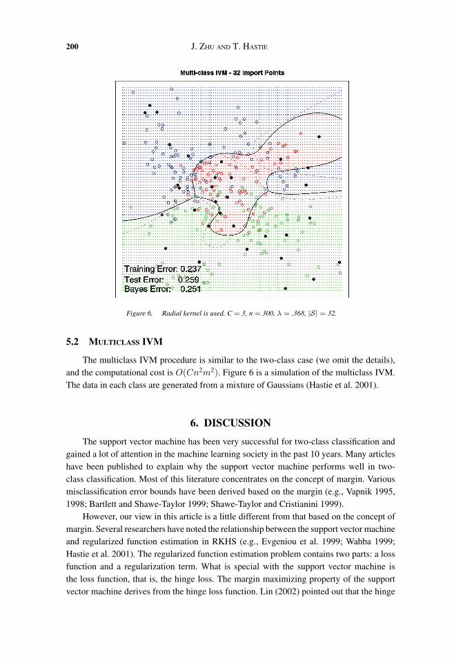
Figure 6. Radial kernel is used. C = 3, n = 300, λ = .368, |S| = 32.

5.2 MULTICLASS IVM

The multiclass IVM procedure is similar to the two-class case (we omit the details),and the computational cost is O(Cn2m2). Figure 6 is a simulation of the multiclass IVM.The data in each class are generated from a mixture of Gaussians (Hastie et al. 2001).

6. DISCUSSION

The support vector machine has been very successful for two-class classification andgained a lot of attention in the machine learning society in the past 10 years. Many articleshave been published to explain why the support vector machine performs well in two-class classification. Most of this literature concentrates on the concept of margin. Variousmisclassification error bounds have been derived based on the margin (e.g., Vapnik 1995,1998; Bartlett and Shawe-Taylor 1999; Shawe-Taylor and Cristianini 1999).

However, our view in this article is a little different from that based on the concept ofmargin. Several researchers have noted the relationship between the support vector machineand regularized function estimation in RKHS (e.g., Evgeniou et al. 1999; Wahba 1999;Hastie et al. 2001). The regularized function estimation problem contains two parts: a lossfunction and a regularization term. What is special with the support vector machine isthe loss function, that is, the hinge loss. The margin maximizing property of the supportvector machine derives from the hinge loss function. Lin (2002) pointed out that the hinge


loss is Bayes consistent, that is, the population minimizer of the loss function agrees withthe Bayes rule in terms of classification. We believe this is a big step in explaining thesuccess of the support vector machine, because it implies the support vector machine istrying to implement the Bayes rule. However, this is only part of the story; we believe thatthe regularization term has also played an important role in the support vector machine’ssuccess.

Regularization is an essential component in modern data analysis, in particular whenthe number of basis functions is large, possibly larger than the number of observations, andnonregularized fitting is guaranteed to give badly overfitted models. The enlarged featurespace in the support vector machine allows the fitted model to be flexible, and the regulariza-tion term controls the complexity of the fitted model; theL2 nature of the regularization termin the support vector machine allows the fitted model to have a finite representation, even ifthe fitted model is in an infinite dimensional space. Hence we propose that by replacing thehinge loss of the support vector machine with the negative binomial log-likelihood, whichis also Bayes consistent, we should be able to get a fitted model that performs similarlyto the support vector machine. The resulting kernel logistic regression is something ourstatisticians are very familiar with (e.g., Green and Yandell 1985; Hastie and Tibshirani1990; Wahba et al. 1995). We all understand why it can work well. The same reasoningcould be applied to the support vector machine. The import vector machine algorithm isjust a way to compress the data and reduce the computational cost.

Kernel logistic regression is not the only model that performs similarly to the supportvector machine, replacing the hinge loss with any sensible loss function will give similarresult, for example, the exponential loss function of boosting (Freund and Schapire 1997),the squared error loss (e.g., Buhlmann and Yu 2001; Zhang and Oles 2001; Mannor, Meir,and Zhang 2002) and the 1/yf loss for distance weighted discrimination (Marron and Todd2002). These loss functions are all Bayes consistent. The negative binomial log-likelihoodand the exponential loss are also margin-maximizing loss functions; but the squared errorloss and the 1/yf loss are not.

To summarize, margin maximization is by nature a nonregularized objective, and solv-ing it in high-dimensional space is likely to lead to overfitting and bad prediction per-formance. This has been observed in practice by many researchers, in particular Breiman(1999). Our conclusion is that margin maximization is not the only key to the support vectormachine’s success; the regularization term has played an important role.

APPENDIX

A.1 PROOF OF THEOREM 1

For the purpose of simple notation, we omit the constant β0 in the proof. We define

G(β) ≡n∑

i=1

ln(

1 + e−yih(xi)T βββ).


Lemma A.1. Consider the optimization problem (2.7)–(2.9), let the solution be de-noted by β(s). If the training data are separable, that is, ∃β, s.t. yih(xi)T β > 0, ∀i, thenyih(xi)T β(s) > 0, ∀i and ‖β(s)‖2 = s for all s > s0, where s0 is a fixed positive number.

Hence,∥∥∥ βββ(s)

s

∥∥∥2

= 1.

Proof: Suppose ∃i∗, s.t. yi∗h(xi∗)T β ≤ 0, then

G(β) ≥ ln(

1 + e−yi∗ h(xi∗ )T βββ)

(A.1)

≥ ln 2. (A.2)

On the other hand, by the separability assumption, we know there exists β∗, ‖β∗‖2 = 1,s.t. yih(xi)T β∗ > 0, ∀i. Then for s > s0 = − ln(21/n − 1)/mini

(yih(xi)T β∗), we have

G(sβ∗) =n∑

i=1

ln(

1 + e−yih(xi)T βββ∗s)

(A.3)

<

n∑i=1

ln 2n

= ln 2. (A.4)

Since G(β(s)) ≤ G(sβ∗), we have, for s > s0, yih(xi)T β(s) > 0, ∀i.For s > s0, if ‖β(s)‖2 < s, we consider to scale up β(s) by letting

β′(s) =

β(s)‖β(s)‖2

s.

Then ‖β′(s)‖2 = s, and

G(β

′(s)

)=

n∑i=1

ln(

1 + e−yih(xi)T βββ′(s)

)(A.5)

<

n∑i=1

ln(

1 + e−yih(xi)T βββ(s))

(A.6)

= G(β(s)

), (A.7)

which is a contradiction. Hence ‖β(s)‖2 = s.

✷

Now we consider two separating candidates β1 and β2, such that ‖β1‖2 = ‖β2‖2 = 1.Assume that β1 separates better, that is:

d1 := mini

yih(xi)T β1 > d2 := mini

yih(xi)T β2 > 0.

Lemma A.2. There exists some s0 = S(d1, d2) such that ∀s > s0, sβ1 incurs smallerloss than sβ2, in other words:

G(sβ1) < G(sβ2).


Proof: Let

s0 = S(d1, d2) =ln n + ln 2d1 − d2

,

then ∀s > s0, we haven∑

i=1

ln(

1 + e−yih(xi)T βββ1s)

≤ n ln(1 + e−s·d1

)(A.8)

≤ n exp(−s · d1) (A.9)

<12

exp(−s · d2) (A.10)

≤ ln(1 + e−s·d2

)(A.11)

≤n∑

i=1

ln(

1 + e−yih(xi)T βββ2s). (A.12)

The first and the last inequalities imply

G(sβ1) < G(sβ2).

✷

Given these two lemmas, we can now prove that any convergence point of βββ(s)s must

be a margin maximizing separator. Assume β∗ is a convergence point of βββ(s)s . Denote

d∗ := mini yih(xi)T β∗. Because the training data are separable, clearly d∗ > 0 (sinceotherwise G(sβ∗) does not even converge to 0 as s → ∞).

Now, assume some β with ‖β‖2 = 1 has bigger minimal margin d > d∗. By continuityof the minimal margin in β, there exists some open neighborhood of β∗:

Nβ∗ = {β : ‖β − β∗‖2 < δ},and an ε > 0, such that:

mini

yih(xi)T β < d − ε, ∀β ∈ Nβββ∗ .

Now by Lemma A.2 we get that there exists some s0 = S(d, d− ε) such that sβ incurssmaller loss than sβ for any s > s0, β ∈ Nβββ∗ . Therefore β∗ cannot be a convergence pointof βββ(s)

s .We conclude that any convergence point of the sequence βββ(s)

s must be a margin maxi-mizing separator. If the margin maximizing separator is unique then it is the only possibleconvergence point, and therefore:

lims→∞

β(s)s

= arg max‖βββ‖2=1

mini

yih(xi)T β.

In the case that the margin maximizing separating hyperplane is not unique, this con-clusion can easily be generalized to characterize a unique solution by defining tie-breakers:if the minimal margin is the same, then the second minimal margin determines which modelseparates better, and so on. Only in the case that the whole order statistics of the margins iscommon to many solutions can there really be more than one convergence point for βββ(s)

s .


ACKNOWLEDGMENTSWe thank Saharon Rosset, Dylan Small, John Storey, Rob Tibshirani, and Jingming Yan for their helpful

comments. We are also grateful for the three reviewers and one associate editor for their comments that helpedimprove the article. Ji Zhu was partially supported by the Stanford Graduate Fellowship. Trevor Hastie is partiallysupported by grant DMS-9803645 from the National Science Foundation, and grant RO1-CA-72028-01 from theNational Institutes of Health.

[Received February 2002. Revised April 2004.]

REFERENCES

Bartlett, P., and Shawe-Taylor, J. (1999), “Generalization Performance of Support Vector Machines and OtherPattern Classifiers,” in Advances in Kernel Methods—Support Vector Learning, eds. B. Schoelkopf, C.Burges, and A. Smola, Cambridge, MA: MIT Press, 43–54.

Bredensteiner, E., and Bennett, K. (1999), “Multicategory Classification by Support Vector Machines,” Compu-tational Optimization and Applications, 12, 35–46.

Breiman, L. (1999), “Prediction Games and Arcing Algorithms,” Neural Computation, 7, 1493–1517.

Buhlmann, P., and Yu, B. (2001), “Boosting With the L2 Loss: Regression and Classification,” Journal of AmericanStatistical Association, 98, 324–340.

Burges, C. (1998), “A Tutorial on Support Vector Machines for Pattern Recognition,” in Data Mining and Knowl-edge Discovery, 2, Boston: Kluwer.

Evgeniou, T., Pontil, M., and Poggio, T. (1999), “Regularization Networks and Support Vector Machines,” inAdvances in Large Margin Classifiers, eds. A. J. Smola, P. Bartlett, B. Scholkopf, and C. Schuurmans,Cambridge, MA: MIT Press, 171–204.

Freund, Y., and Schapire, R. (1997), “A Decision-Theoretic Generalization of On-line Learning and an Applicationto Boosting,” Journal of Computer and System Sciences, 55, 119–139.

Green, P., and Yandell, B. (1985), “Semi-parametric Generalized Linear Models,” Proceedings 2nd InternationalGLIM Conference, Lancaster, Lecture notes in Statistics No. 32, New York: Springer, pp. 44–55.

Hastie, T., and Tibshirani, R. (1990), Generalized Additive Models, New York: Chapman and Hall.

Hastie, T., Tibshirani, R., and Friedman, J. (2001), The Elements of Statistical Learning. New York: Springer.

Kaufman, L. (1999), “Solving the Quadratic Programming Problem Arising in Support Vector Classification,”in Advances in Kernel Methods—Support Vector Learning, eds. B. Scholkopf, C. Burges, and A. Smola,Cambridge, MA: MIT Press, 147–168.

Keerthi, S., Duan, K., Shevade, S., and Poo, A. (2002), “A Fast Dual Algorithm for Kernel Logistic Regression,”International Conference on Machine Learning, 19.

Kimeldorf, G., and Wahba, G. (1971), “Some Results on Tchebycheffian Spline Functions,” Journal of Mathe-matical Analysis and Applications, 33, 82–95.

Lee, Y., Lin, Y., and Wahba, G. (2004), “Multicategory Support Vector Machines, Theory, and Application to theClassification of Microarray Data and Satellite Radiance Data,” Journal of American Statistical Association,99, 67–81.

Lin, Y. (2002), “Support Vector Machines and the Bayes Rule in Classification,” Data Mining and KnowledgeDiscovery, 6, 259–275.

Lin, X., Wahba, G., Xiang, D., Gao, F., Klein, R., and Klein B. (2000), “Smoothing Spline ANOVA Models forLarge Data Sets with Bernoulli Observations and the Randomized GACV,” The Annals of Statistics, 28,1570–1600.

Luo, Z., and Wahba, G. (1997), “Hybrid Adaptive Splines,” Journal of American Statistical Association, 92,107–116.


Mannor, S., Meir, R., and Zhang, T. (2002), “The Consistency of Greedy Algorithms for Classification,” inProceedings of the European Conference on Computational Learning Theory, pp. 319–333.

Marron, J., and Todd, M. (2002), “Distance Weighted Discrimination,” Technical Report No. 1339, School ofOperations Research and Industrial Engineering, Cornell University.

Platt, J. (1999), “Fast Training of Support Vector Machines using Sequential Minimal Optimization,” in Advancesin Kernel Methods—Support Vector Learning, eds. B. Scholkopf, C. Burges, and A. Smola, Cambridge, MA:MIT Press.

Ratsch, G., Onoda, T., and Muller, K. (2001), “Soft Margins for Adaboost,” Machine Learning, 42, 287–320.

Rosset, S., Zhu, J., and Hastie, T. (2004), “Margin Maximizing Loss Functions,” Neural Information ProcessingSystems, 16.

Shawe-Taylor, J., and Cristianini, N. (1999), “Margin Distribution Bounds on Generalization, in Proceedings ofthe European Conference on Computational Learning Theory, 263–273.

Smola, A., and Scholkopf, B. (2000), “Sparse Greedy Matrix Approximation for Machine Learning,” in Pro-ceedings of the Seventeenth International Conference on Machine Learning, San Francisco, CA: MorganKaufmann, 911–918.

Vapnik, V. (1995), The Nature of Statistical Learning Theory, Berlin: Springer Verlag.

(1998), Statistical Learning Theory, New York: Wiley.

Wahba, G. (1999), “Support Vector Machines, Reproducing Kernel Hilbert Spaces and the Randomized GACV,”in Advances in Kernel Methods—Support Vector Learning, eds. B. Scholkopf, C. Burges, and A. Smola, Cambridge, MA: MIT Press, 69–88.

Wahba, G., Gu, C., Wang, Y., and Chappell, R. (1995), “Soft Classification, a.k.a. Risk Estimation, via PenalizedLog-Likelihood and Smoothing Spline Analysis of Variance,” in The Mathematics of Generalization, ed.D. H. Wolpert, Santa Fe Institute Studies in the Sciences of Complexity, Reading, MA: Addison-Wesley,329–360.

Weston, J., and Watkins, C. (1999), “Support Vector Machines for Multiclass Pattern Recognition,” in Proceedingsof the Seventh European Symposium on Artificial Neural Networks.

Williams, C., and Seeger, M. (2001), “Using the Nystrom Method to Speed up Kernel Machines,” in Advances inNeural Information Processing Systems 13, eds. T. K. Leen, T. G. Diettrich, and V. Tresp, Cambridge, MA:MIT Press, pp. 682–688.

Zhang, T., and Oles, F. (2001), “Text Categorization Based on Regularized Linear Classification Methods,” Infor-mation Retrieval, 4, 5–31.

Zhu, J., and Hastie, T. (2004), “Classification of Gene Microarrays by Penalized Logistic Regression,” Biostatistics,25, 427–444.

Download - Kernel Logistic Regression and the Import Vector …dept.stat.lsa.umich.edu/~jizhu/pubs/Zhu-JCGS05.pdf · Kernel Logistic Regression and the Import Vector Machine ... Recently Keerthi,

Top Related