Download - ISBN 978-952-15-0279-7 (printed) ISBN 978-952-15-4216-9 (PDF)

ISBN 978-952-15-0279-7 (printed)ISBN 978-952-15-4216-9 (PDF)ISSN 0356-4940

Abstract

In this study, a simple method was developed for reducing noise during theiterative reconstruction of emission tomography images.

The emission images express the spatial distribution of a chemical com-pound, if possible in quantitative terms. The concentration of the tracer givesinformation about the active metabolism of a living tissue. As a computa-tional medical imaging method, the emission tomography involves a significantamount of data processing. The algorithms that carry out the computation ofthe estimate of the transaxial image from the measured data suffer from noisedue to the statistical nature of the acquisition.

The new method (MRP, median root prior) is novel and generally applicablefor emission reconstruction, independent of the organ or the tracer. The prin-ciple of penalizing locally non-monotonic noise is suitable for both emissionand transmission image reconstruction. Instead of explicitly producing visuallypleasing images, the method is designed to compute locally accurate imageswith no constraints on pixel value differences.

In practice, MRP is quantitatively accurate and simple in implementation.The transmission reconstruction with this method allows for a short-time atten-uation correction. As a result of this, the scanning time for the patient can bereduced.

i

ii ABSTRACT

PrefaceThis work has been done in the Signal Processing Laboratory of Tampere

University of Technology in a close cooperation with Turku PET Centre, Tam-pere University Hospital, and Kuopio University Hospital.

I thank my supervisor Prof. Jaakko Astola for valuable advice. I owe mydeepest gratitude especially to Ph.D. Ulla Ruotsalainen for leading me into theworld of PET and for pointing out the essential point of view.

I thank the preliminary assessors of this dissertation, Prof. Johan Nuyts andAssoc. Prof. Jeffrey Fessler, for their thorough work.

I express my sincere thanks to the personnel of Turku PET Centre for pro-viding an exiting environment for both business and pleasure. I thank Prof.Juhani Knuuti, Ph.D. Chietsugu Katoh, Ph.D. Tapio Utriainen, and M.D. MeriKahkonen for linking my work to the medical field, where I am a mere layman.Thanks to Lic.Tech. Paivi Laarne, M.Sc. Vesa Oikonen, and Mr. Mika Klemetsoother people can use some of my programs in their work. I am thankful to thephysicists M.Sc. Mika Teras, M.Sc. Tuula Tolvanen, and B.Sc. Petri Numminenfor carrying out important tasks when implementing MRP.

I am grateful to Ph.D. Matti Koskinen and Ph.D. Antti Virjo in TAUH andLic.Sc. Tomi Kauppinen in KUH for broadening the scope of the applicationfrom PET to SPECT by working hard with a professional attitude.

I thank my fellow workers in TUT/DMI/SPAG/MFGI for an enjoyable andrelaxed atmosphere I have been privileged to share. I extend my thanks also tothe personnel of Tampere Image Processing Systems for bringing me into theprofessional life during the early years of my career.

The financial support provided by the City of Tampere, the Ulla TuominenFoundation, the Research Foundation of Instrumentarium, Tampere GraduateSchool in Information Science and Engineering, and the Research Scholar-ship Found of Tampere (Tamperelaisen tutkimustyon tukisaatio) is gratefullyacknowledged.

I thank my closest family for support and especially my nieces Marika andPauliina for giving delight to my life. The other Pauliina deserves my warmestthanks for moments not related to this thesis.

Tampere, August 1999Sakari Alenius

iii

iv PREFACE

Contents

Abstract i

Preface iii

List of publications ix

Symbols and abbreviations xi

1 Introduction 11.1 Objectives of emission tomography . . . . . . . . . . . . . . 11.2 Problems in the image reconstruction . . . . . . . . . . . . . . 31.3 Structure of the work . . . . . . . . . . . . . . . . . . . . . . 4

2 Data Acquisition 52.1 PET emission . . . . . . . . . . . . . . . . . . . . . . . . . . 52.2 PET transmission . . . . . . . . . . . . . . . . . . . . . . . . 6

2.2.1 Attenuation correction . . . . . . . . . . . . . . . . . 72.3 SPECT . . . . . . . . . . . . . . . . . . . . . . . . . . . . . 82.4 Noise and errors in data . . . . . . . . . . . . . . . . . . . . . 10

3 Image Reconstruction 113.1 Filtered back projection . . . . . . . . . . . . . . . . . . . . . 11

3.1.1 The Radon transform and its inverse . . . . . . . . . . 113.1.2 Applicability to PET . . . . . . . . . . . . . . . . . . 14

3.2 On iterative reconstruction algorithms . . . . . . . . . . . . . 163.2.1 Notations . . . . . . . . . . . . . . . . . . . . . . . . 163.2.2 General concept . . . . . . . . . . . . . . . . . . . . 17

3.3 Maximum likelihood . . . . . . . . . . . . . . . . . . . . . . 183.3.1 MLEM algorithm . . . . . . . . . . . . . . . . . . . . 183.3.2 Noise and bias in iterations . . . . . . . . . . . . . . . 21

3.4 Bayes priors and penalties . . . . . . . . . . . . . . . . . . . 223.4.1 Gibbs priors . . . . . . . . . . . . . . . . . . . . . . . 23

v

vi CONTENTS

3.4.2 One step late algorithm . . . . . . . . . . . . . . . . . 243.4.3 Mathematical priors . . . . . . . . . . . . . . . . . . 253.4.4 Anatomical priors . . . . . . . . . . . . . . . . . . . . 28

3.5 Implementational aspects . . . . . . . . . . . . . . . . . . . . 293.5.1 Acceleration techniques . . . . . . . . . . . . . . . . 293.5.2 Corrections . . . . . . . . . . . . . . . . . . . . . . . 30

3.6 Performance measures of estimators . . . . . . . . . . . . . . 303.7 Summary . . . . . . . . . . . . . . . . . . . . . . . . . . . . 31

4 Aims of the work 33

5 Median Root Prior 355.1 General description . . . . . . . . . . . . . . . . . . . . . . . 355.2 MRP Algorithm . . . . . . . . . . . . . . . . . . . . . . . . . 36

5.2.1 Emission OSL algorithm . . . . . . . . . . . . . . . . 365.2.2 Interpretations on the prior . . . . . . . . . . . . . . . 36

5.3 Transmission algorithm . . . . . . . . . . . . . . . . . . . . . 385.3.1 Motivation . . . . . . . . . . . . . . . . . . . . . . . 385.3.2 Data fitting algorithm . . . . . . . . . . . . . . . . . . 395.3.3 tMRP algorithm . . . . . . . . . . . . . . . . . . . . 40

5.4 On convergence properties . . . . . . . . . . . . . . . . . . . 415.5 Noise and bias . . . . . . . . . . . . . . . . . . . . . . . . . . 415.6 Implementation . . . . . . . . . . . . . . . . . . . . . . . . . 41

5.6.1 Neighborhood size . . . . . . . . . . . . . . . . . . . 415.6.2 Parameterβ . . . . . . . . . . . . . . . . . . . . . . . 425.6.3 Iterations . . . . . . . . . . . . . . . . . . . . . . . . 42

6 Results and Images 456.1 Simulations . . . . . . . . . . . . . . . . . . . . . . . . . . . 45

6.1.1 Error histograms . . . . . . . . . . . . . . . . . . . . 466.1.2 Reliability of ROI estimation . . . . . . . . . . . . . . 486.1.3 Noise sensitivity . . . . . . . . . . . . . . . . . . . . 496.1.4 Parameter sensitivity . . . . . . . . . . . . . . . . . . 496.1.5 Images . . . . . . . . . . . . . . . . . . . . . . . . . 52

6.2 Clinical data . . . . . . . . . . . . . . . . . . . . . . . . . . . 536.2.1 Emission studies . . . . . . . . . . . . . . . . . . . . 536.2.2 Transmission . . . . . . . . . . . . . . . . . . . . . . 556.2.3 Whole body studies . . . . . . . . . . . . . . . . . . . 56

6.3 SPECT images . . . . . . . . . . . . . . . . . . . . . . . . . 576.4 Summary of results and the publications . . . . . . . . . . . . 58

CONTENTS vii

7 Discussion 617.1 General principle . . . . . . . . . . . . . . . . . . . . . . . . 617.2 Applicability of MRP . . . . . . . . . . . . . . . . . . . . . . 637.3 Conclusion . . . . . . . . . . . . . . . . . . . . . . . . . . . 64

Bibliography 65

Publications 75

viii CONTENTS

List of publications

I : S. Alenius. Bayesian Image Reconstruction in Positron Emission Tomog-raphy using Median Root Prior.The Proceedings of the First TUT Sym-posium on Signal Processing ‘94, pp. 113-116, 1994, Tampere, Finland.

II : S. Alenius, U. Ruotsalainen. Bayesian image reconstruction for emissiontomography based on median root prior.European Journal of NuclearMedicine,vol. 24, pp. 258-265, Mar 1997.

III : S. Alenius, U. Ruotsalainen, J. Astola. Using local median as the lo-cation of the prior distribution in iterative emission tomography imagereconstruction.IEEE Transactions on Nuclear Science,selected papersfrom the 1997 Medical Imaging Conference (MIC), Albuquerque, NewMexico, November 13-15 1997, vol. 45, no. 6(2), pp. 3097-3107, Dec1998.

IV : S. Alenius, U. Ruotsalainen, and J. Astola. Attenuation Correction forPET Using Count-Limited Transmission Images Reconstructed with Me-dian Root Prior.IEEE Transactions on Nuclear Science,selected papersfrom the 1998 Medical Imaging Conference (MIC), Toronto, Canada,November 11-14 1998, vol. 46, no. 3(2), pp. 646-651, June 1999.

ix

x LIST OF PUBLICATIONS

Symbols and abbreviations

β Bayes weightC constant, terms independent of the variable in questionδ() Dirac delta functionFn{} n-dimensional Fourier transformλ emission imageµ transmission imageR{} Radon transform

ACF attenuation correction factorART algebraic reconstruction techniqueBq Bequerel, unit of activity, one disintegration per second(1/s)CT computerized (computed) tomographyET emission tomographyeV electron volt, unit of energyFBP filtered back projectionFDG fluoro-2-deoxy-D-glucoseFFT fast Fourier transformFIR finite impulse responseFOV field of viewFT Fourier transformLOR line of responseMAE mean absolute errorMAP maximuma posterioriML maximum likelihoodMLEM maximum likelihood expectation maximizationMRF Markov random fieldMRI magnetic resonance imagingMRP median root priorMSE mean squared errorOSL one step latePDF probability density functionPET positron emission tomography

xi

xii SYMBOLS AND ABBREVIATIONS

PSF point spread functionROI region of interestRT Radon transformSPECT single photon emission computed tomography, a.k.a. SPETSPET single photon emission tomography, a.k.a. SPECTtMRP transmission MRP

Chapter 1

Introduction

1.1 Objectives of emission tomography

Tomography (Greektomos= section, + -graphy) means a method of produc-ing an image of the internal structures of a solid object by the observation andrecording of the differences in the effects on the passage of waves of energyimpinging on those structures [64]. The medical applications of tomographyutilize the non-invasive nature of the procedure, which makes it possible to ex-amine living objectsin vivo. Different tomographic imaging modalities providedifferent kind of information depending on the data recording means. The tradi-tional X-ray based computerized tomography (CT) produces images of photonattenuation in the tissue, and magnetic resonance imaging (MRI) describes theproton or water density [45]. These images are generally anatomical becausethey reveal the physical structure of the tissue, serving as an ”electronic knife”.Such properties as the density of the tissue, the water density, and the membranestructure are examples of objects of interest in the anatomical imaging.

Emission tomography (ET) is intended to express functional properties ofthe tissue. Emission refers to the fact that the energy source is not external butit is brought into the tissue as a part of the body metabolism. This is done bya tracer which is a chemical compound labeled with a radioactive isotope. Thespatial distribution of the radiating source is the object of interest as it tells theconcentration of the tracer in the tissue. As the labeled compound is chemicallyidentical to its non-labeled counterpart, an image of the spatial source distribu-tion shows information about the metabolism relating to the compound duringthe data acquisition period. Thus, functional ET images are generally differentfrom anatomical images. Primarily, ET images do not express what the tissuelooks like, but how it functions. Although functional and anatomical images ofthe same organ have some similarities, such as boundaries between tissue types(see Fig. 1.1), the essential information in an ET image is where it differs from

1

2 CHAPTER 1. INTRODUCTION

the corresponding anatomical image. An ET image can be used when studyingthe normal behavior of the tissue, or when diagnosing abnormal cases in clini-cal work. The main areas of medicine that utilize ET are neurology, cardiology,and oncology.

(a) Photo (b) CT (c) MRI(T1)

(d) MRI(T2) (e) PET (f) SPECT

Figure 1.1: Examples of various imaging modalities. Images are not of the sameperson. Sources: [12], [43], Turku PET Centre, and Kuopio University Hospital.

Tomographic images as slices are originally two-dimensional, but they canbe combined to a 3D image. What is more, a time sequence of ET images forma dynamic 3D or 4D image. The dimension of time is medically important be-cause the concentration of the tracer in the tissue changes in time. A parametricimage computed from a dynamic image sequence depicts values of a certainmetabolic rate as an image [73].

There are two ET modalities that share some common properties. Positron

1.2. PROBLEMS IN THE IMAGE RECONSTRUCTION 3

emission tomography (PET) is capable to quantitative measurements of tracerradioactivity concentration. Simpler and cheaper single photon emission com-puted tomography (SPECT, a.k.a. SPET) has traditionally been used for relativemeasurements.

1.2 Problems in the image reconstruction

The measured data in tomography are not an image of the object, but projectionsof it, a sinogram. The unknown image has to be estimated from the availabledata computationally. This task is called the image reconstruction from projec-tions [37]. Its goal is a reasonably accurate image with a reasonably low noiselevel. The ET data acquisition is subject to a substantial amount of statisticalnoise, originating from the statistical nature of the decay of the label isotope.Fig. 1.2(a) shows a PET sinogram. The noise in the sinogram contributes toreconstruction artifacts visible in the reconstructed image of the object 1.2(b).

(a) Sinogram (b) Reconstructed object

Figure 1.2: A PET sinogram and the reconstructed image. Both are shown asnegative pictures.

The accuracy of the image reconstruction is the basis of ET studies. The re-gion of interest (ROI) analysis is based on determining the activity in the tissueaveraged over selected set of image pixels. Noise and reconstruction artifactsdeteriorate the reliability of the ROI analysis in two ways. First, the ROI is diffi-cult to draw on an image with reconstruction artifacts and noise. Secondly, theymay cause some local bias to the quantitative values of ROI pixels. Because the

4 CHAPTER 1. INTRODUCTION

dose given to the patient should be fairly low and the acquisition time shouldbe relatively short, the noise level of the acquired data is unavoidably quitehigh. Thus, there is a need for improvement of the quality of the reconstructedimages.

Image enhancement and filtering methods that are convenient in generalpurpose image processing may not serve as reliable noise reduction means inET. Particularly the quantitative accuracy of PET sets special requirements toimage improvement operations. What is more, the image reconstruction processitself should take advantage of the special nature of image formation process.The system’s sensitivity in distinguishing between two different activity levelsshould not be compromised by the noise reduction operation. Also, the reso-lution of how well two neighboring areas of different activity can be separatedspatially should be maintained.

1.3 Structure of the work

The main result of this work is a practical way to remove a significant amountof noise during the iterative reconstruction process without causing substantialbias and without removing relevant information. The developed method is gen-eral and simple, it applies to various iterative reconstruction algorithms, and itcan be used independently of the organ under the study. The main focus is inPET.

Chapter 2 addresses the data acquisition process. The principles of the emis-sion detection are discussed. The basis of quantitative measurements, the at-tenuation correction, is shortly described. The differences between PET andSPECT and the noise contamination in the data are discussed, too.

Chapter 3 discusses two main classes of image reconstruction methods, an-alytical and statistical algorithms. Various approaches for noise reduction ofthe iterative algorithms are reviewed.

Chapter 4 presents the main goals of the work.Chapter 5 describes the main contribution of the author, the MRP algorithm.

MRP is used in conjunction with an iterative algorithm as a regularizer or apenalty.

Chapter 6 reports results and experiments of MRP reconstructions appliedboth on simulated and on clinical data.

Chapter 7 draws conclusions about the relevance of MRP in the field ETimage reconstruction.

Chapter 2

Data Acquisition

2.1 PET emission

In PET, common labels are11C, 13N , 15O, and18F isotopes [80]. They can beattached to medically interesting molecules by radiopharmaceutical processes.The tracer can be introduced into the patient by injection or by inhalation. Thenucleus of the label is unstable and it transforms into a stable isotope by emit-ting a positron. The positron and the electron are anti-particles. Their massesannihilate into two photons of 511 keV according to the equationE = mc2

[7]. That energy is enough for escaping the body. Because the photons travel atalmost opposing directions, the data acquisition is accomplished by detectingcoincident events by a detector ring surrounding the patient (Fig. 2.1). Eachevent is recorded related to a line of response (LOR), a line along which theannihilation took place. The area overlapped and enclosed by the LORs is thefield of view (FOV). The angles and the positions of the LORs are saved as 2Dtables, sinograms. Each row of the sinogram corresponds to a projection profileat certain angle, and the bins of the row correspond to the detector pairs on thatdirection. A point source generates half of a sine wave into the sinogram, asvisible in Fig. 1.2 on page 3. After the measurement interval, each sinogrambin contains the number of detected events (counts) for its LOR.

The reconstructed image is a temporal average of the spatial tracer distri-bution on the transaxial image plane over the data acquisition period. Theunit of quantitative images is commonly kBq/ml. Quantitative accuracy canbe achieved by elimination the effect of the body attenuation and scatter. Eventhough transmittance properties are not the main interest in PET, the transmis-sion measurements are carried out in order to get quantitative images.

5

6 CHAPTER 2. DATA ACQUISITION

ringDetector

bin

Sinogram

L2

L1

d angle

increment count

e− + e+ = 2γ

µ

Figure 2.1: Photon acquisition in PET. The detectors work in pairs registeringcoincidentγ-photons. The sinogram contains the registered counts. The attenuationeffect is independent of the position of the annihilation.

2.2 PET transmission

The emitted photon may interact with the matter and scatter from its originalfly path. If that happens, no true coincident event occurs. Thus, not all an-nihilations are detected as the body attenuates the photon flux. The photonattenuation has to be taken into consideration in order to find out the spatialemission source distribution quantitatively. Also, an image of the transmittanceproperties of the tissue may be useful in some studies [11].

The probability that both of the emitted photons travel without scattering tothe detectors is [45]

P = P1P2 = e− ∫L1d

µ(x)dxe− ∫L2d

µ(x)dx= e

− ∫Ldµ(x)dx , e−ad , (2.1)

whereµ is the 2D function of linear mass absorption coefficients,Ld is the pathcorresponding to LOR for detector paird, andL1d andL2d are the sub-pathsfrom the place of annihilation to detectors (Ld = L1d +L2d, Fig. 2.1). Becauseof the coincidence detection, the attenuation effect ond is independent of theposition of the annihilation along the LOR. This is why an external source canbe used when measuring the attenuation of the body.

2.2. PET TRANSMISSION 7

2.2.1 Attenuation correction

Measured attenuation correction

In order to determine the attenuation of the body, two additional measurementsare done: the blank scan and the transmission scan [41]. The blank scan isrecorded using an external source without the patient. This represents the unat-tenuated case. For the transmission scan the patient and the bed are placed intothe scanner and the attenuated data are measured using the external source. Theexternal source can be ring-shaped on a fixed position, or a rotating line or pointsource [11].

The attenuation correction factor (ACF) can be calculated as the ratio of themeasured counts without and with the attenuating object

ACF d =Bd e0

Bd e−ad= ead , (2.2)

whereBd is the measured activity of the external source. The ACFs form asinogram, whose elements express the amount of attenuation for the detectorpaird. Figure 2.2 shows the two scans and the resulting ACFs. Attenuation pre-correction is carried out as the multiplication of the emission sinogram countby the corresponding ACF. The ACF in Eq. (2.2) is intended to cancel out theattenuation expressed by Eq. (2.1).

(a) Blank (b) Transmission (c) ACF

Figure 2.2: The smoothed blank scan, the smoothed transmission scan, and theattenuation correction factors according to (2.2) shown as negative pictures.

Short transmission scan times increase the noise level and worsen the qual-ity of ACFs. Due to noise, the scan data are usually smoothed prior to the


division. Otherwise the noise in the ACFs propagates to the corrected emissionsinogram. The drawback of smoothing is that the resulting blurring of ACFspropagates to the emission sinogram as well [19].

The measurement of the transmission data can be done before the emis-sion acquisition, which increases the time spent in clinical routines. In orderto reduce the patient discomfort, the transmission acquisition can be done si-multaneously to the emission scan by utilizing a dedicated hardware design.Consequently, the cross contamination of the transmission data and the emis-sion data must be taken care of [11].

Computational attenuation correction

If the transmission acquisition must be avoided, attenuation correction can beperformed by computational methods [41]. The attenuating matter is approxi-mated by an area with a uniform value of linear mass absorption coefficientµ.The ACFs can be computed by projecting the graphically definedµ-image andtaking the exponential

ACF d = e∫

Ldµ(x)dx

. (2.3)

The assumption that theµ-values are uniform and the manual work usuallyrequired restrict the usage of (2.3) [41].

Hybrid attenuation correction

The hybrid methods for attenuation correction combine the transmission mea-surements and the computational method [41]. First, theµ-image is recon-structed from the natural logarithm of the ACFs (2.2). Then this transmissionimage is segmented to assumed tissue types. The pixel values in the segmentedareas are assigned with the known averageµ-values and the resulting image isprojected to ACFs (2.3). The segmentation step reduces the noise in the trans-mission from propagating to the emission scan when the emission sinogram aremultiplied with the ACFs. The assumptions that there is a known number of tis-sue types and that they are uniform limit the applicability of the hybrid methodwith organs with diverse set ofµ-values, as lungs [77].

2.3 SPECT

SPECT devices register only single photons usually without any coincidencedetection [42]. This allows for detection of photons of various energy levels,not only those produced by the positron annihilation. Commonly used labels

2.3. SPECT 9

are 99mTc and 201T l. In the absence of the coincidence detection, a physicalcollimation is required in order to restrict the possible ray path of photons en-tering the detector. Usually the detector heads (one, two or three) can be rotatedmechanically around the patient. Each head contains a matrix of detectors suchthat the head records an image at its rotational position. These images can beused as planar images without the reconstruction. The counts along a transver-sal line of the acquisition images form the sinogram, as shown in Fig. 2.3. Thereconstruction of the sinogram gives the image of the selected transaxial slice.

Figure 2.3: An emission SPECT study of a brain.Left : The acquisition image.Right: The sinogram with full 360◦ rotation. The projections 180◦ apart can becombined before the reconstruction.

Often there are no attenuation correction used in SPECT. Without the co-incidence detection the attenuation depends on the depth of the source locationin the object. Each detector collects photons originating from various depthsand the total count cannot be compensated by a single factor, even if the oppos-ing counts are combined [79]. The measured attenuation correction in SPECTcan be accomplished in a similar way than in PET, but the pre-correction (2.2)is only approximate [41, 11]. For quantitative results, the sketched or recon-structedµ-image can be used for computing the attenuated projections insidethe emission reconstruction algorithm [11].

The lack of the attenuation correction makes SPECT studies commonlynon-quantitative, and the visual quality of the reconstructed image is more im-portant. Sometimes pre-filtering is applied on the acquired data or post-filteringon the reconstructed images.


2.4 Noise and errors in data

The data acquisition process in ET measures the product of the radioactive de-cay, which is a random process. The emission of a positron is a rare event,but in a large population (high number of atoms) the number of such events isdistributed according to Poisson distribution [70].

An underlying activity generates a random number of disintegrations pera time interval. The realized number of events (counts),n, is drawn froma Poisson distribution with the mean equal to the underlying activityλ [76],Poisson(λ)

P{n = λ} = e−λ λn

n!. (2.4)

Technically speaking, the main interest in ET is to estimate the unknownmean activityλ.

In addition to the statistical noise, the data acquisition system results insome errors in the data because of the finite energy and time resolution of thedetectors. If the photon isscattered, it can still be accepted by a detector, whichresults a LOR with no real annihilation. Also, almost simultaneous single pho-tons can be accepted as a pair, which accounts for anaccidentalcoincident.The detectors have individual gains, which must benormalized. There is adead timeafter each event before the detector is able to record again. Photonsarriving during that time are lost. The positron travels a few millimeters in thetissue loosing some energy before it can interact with an electron. The distancebetween the place of the annihilation and the place of the decay is thepositronrange, which contributes to the point spread function (PSF) of the device. Theseerrors can be partly compensated by approximate statistical methods prior to orduring the reconstruction. However, the Poisson nature of the noise in the datamay be distorted by the operations applied on the raw data [72, 85].

Chapter 3

Image Reconstruction

The image reconstruction process computes a 2D slice of the object emittingradiation, or in the transmission case, exposed to radiation. The measured ra-diation profiles organized as a sinogram are the input to the reconstruction. Asan inverse problem the reconstruction is to some extent similar to the imagerestoration, but the main difference is the transform from the projection spaceinto the image space.

The noise and the finite amount of measured data make the reconstructedimage only an approximation of the true object. The properties of the imagedepend on the choice of the reconstruction method. The main differences be-tween reconstruction methods come from how the data and the acquisition aremodeled.

3.1 Filtered back projection

3.1.1 The Radon transform and its inverse

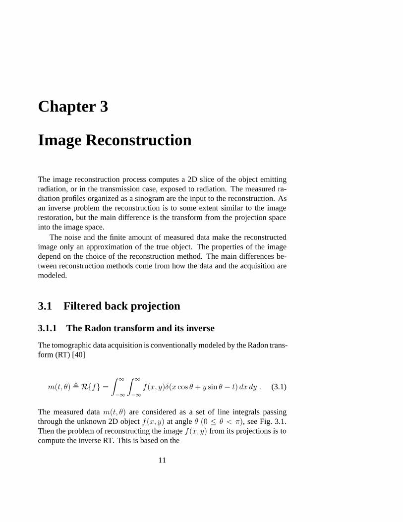
The tomographic data acquisition is conventionally modeled by the Radon trans-form (RT) [40]

m(t, θ) , R{f} =

∫ ∞

−∞

∫ ∞

−∞f(x, y)δ(x cos θ + y sin θ − t) dx dy . (3.1)

The measured datam(t, θ) are considered as a set of line integrals passingthrough the unknown 2D objectf(x, y) at angleθ (0 ≤ θ < π), see Fig. 3.1.Then the problem of reconstructing the imagef(x, y) from its projections is tocompute the inverse RT. This is based on the

11

12 CHAPTER 3. IMAGE RECONSTRUCTION

Fourier slice theorem: The 1D Fourier transform of a projectiontaken at angleθ equals the central radial slice at angleθ of the 2DFourier transform of the original object.[40, 45]

The Fourier slice theorem can be proved in a following way. A projectionprofile is expressed using a rotated coordinate system(t, s)

[ts

]=

[cos θ sin θ− sin θ cos θ

] [xy

],

[xy

]=

[cos θ − sin θsin θ cos θ

] [ts

];

(3.2)and (3.1) can be written as

m(t, θ) =

∫ ∞

−∞f(t cos θ − s sin θ, t sin θ + s cos θ) ds . (3.3)

Using (3.3), the 1D Fourier transform (FT) ofm(t, θ) with respect tot is

F1{m(t, θ)} , M(ω, θ) =

∫ ∞

−∞m(t, θ) e−j2πωtdt

=

∫ ∞

−∞

∫ ∞

−∞f(t cos θ − s sin θ, t sin θ + s cos θ) e−j2πωt dt ds

=

∫ ∞

−∞

∫ ∞

−∞f(x, y) e−j2πω(x cos θ+y sin θ)

∣∣∣∣∣∂t∂x

∂s∂x

∂t∂y

∂s∂y

∣∣∣∣∣︸︷︷︸cos2 θ+sin2 θ=1

dx dy

= F (ω cos θ, ω sin θ) , (3.4)

whereF (u, v) = F2{f(x, y)}, andω is the frequency variable of the 1D FT.(3.4) gives the values of the 2D FT evaluated along the line(u = ω cos θ, v =ω sin θ) across the(u, v) space.

The Fourier slice theorem states that if the 2D Fourier space could be filled,the inverse 2D FT would give the original object. This is illustrated in Fig. 3.1.Unfortunately, a discrete implementation of (3.4) using fast Fourier transforms(FFT) requires interpolations especially at the high frequencies, where the den-sity of the resulting 2D Fourier space is low. This is why direct Fourier methodsare not popular as inverse Radon transform algorithms [37]. The most commonalgorithm for the inverse RT is the filtered back projection (FBP) [45], which isdescribed next.

3.1. FILTERED BACK PROJECTION 13

s

t

x

other projections1D FT

2D FT

1D FT of

u

y v

projection

object

θ

Figure 3.1: The relation of the image space, the Radon space, and the Fourier spaceaccording to the Fourier slice theorem.

The inverse 2D FT expressed using the polar coordinatesω and θ in thefrequency space(u = ω cos θ, v = ω sin θ) is

f(x, y) = F−12 {F (u, v)} =

∫ ∞

−∞

∫ ∞

−∞F (u, v) ej2π(xu+yv) du dv

=

∫ 2π

0

∫ ∞

0

F (ω cos θ, ω sin θ) ej2πω(x cos θ+y sin θ)

∣∣∣∣∣∂u∂ω

∂v∂ω

∂u∂θ

∂v∂θ

∣∣∣∣∣︸︷︷︸=ω

dω dθ

=

∫ π

0

[∫ ∞

−∞M(ω, θ)|ω| ej2πω(x cos θ+y sin θ) dω

]dθ

=

∫ π

0

m(x cos θ + y sin θ, θ) dθ , B {m(t, θ)} , (3.5)

where the Fourier slice theorem (3.4) and the definitionm(t, θ) ,∫∞−∞ M(ω, θ)

|ω| ej2πωt dω were used. The multiplication by|ω| serves as a filter applied toeach projection profile in the frequency space. The filtered profilem is summedalong the ray paths to the image space. The notationB {m(t, θ)} is the backprojection ofm over the image. Now (3.5) gives an algorithm to reconstruct theimagef(x, y) from its projectionsm(t, θ):

Filtered back projection, FBP: Setf(x, y) = 0,∀x, y. For eachprojection profile:


• Take FT

• Apply the frequency domain filter

• Take inverse FT

• Back project over the image at the given angle

In the discrete implementation of FBP, the integrals are replaced by finitesummations and FFTs can be used. The filtering can be performed also as aconvolution in the spatial domain, giving the alternative algorithm called theconvolution – back projection [60]. The back projection step requires interpo-lation, which is the most time consuming part of the algorithm. Otherwise, FBPis fast and simple in implementation.

3.1.2 Applicability to PET

FBP is capable to compute accurately the inverse Radon transform. FBP workswell especially in the transmission tomography (CT), where the radiation sourceand the detector are on the opposing sides of the object. In the emission tomog-raphy the source is introduced into the object. The measured radiation profilesare organized as a sinogram, and FBP can be used for the emission case, too.Attenuation correction can be applied to the emission sinogram before the re-construction. However, in ET the measured data are intrinsically noisy, and RTis not an accurate model for the measurement process. This is why the inverseRT image provided by FBP suffers from heavy noise. FBP is especially sensi-tive to noise because the ramp filter|ω| in (3.5) amplifies high frequencies. Thiseffect can be weakened by applying a window function to the ramp filter (Fig.3.2) [36].

A cutoff frequencyωc can also be used as a truncation threshold for elimi-nating high frequencies. Including the windowWωc(ω), FBP becomes

f(x, y) =

∫ π

0

[∫ ∞

−∞M(ω, θ) |ω|Wωc(ω) ej2πω(x cos θ+y sin θ) dω

]dθ . (3.6)

Because the frequency bands of the true signal and noise overlap, a trade-offbetween the resolution and noise rejection is unavoidable. This compromise istuned by the filter function and the cutoff. The reconstruction artifacts of ETimages reconstructed by FBP are most prominent in the background, where thecorrect value should be zero. The radial streaks are due to the fact that filterednoisy projection profiles do not cancel out each others in the back projection.This results in both positive and negative background pixel values. What ismore, the back projection smears each profile over the entire image, and theartifacts are not necessarily canceled out in any part of the image.

3.1. FILTERED BACK PROJECTION 15

Figure 3.2: Common filter functions for FBP.

The noise in the data originating from a local radioactive decay processcontributes over a large spatial area of the image reconstructed by the FBPalgorithm. This makes the bias of a ROI not independent of the rest of theimage. For instance, the noise and the quantitative value of a low-activity areamay depend on whether there is a high activity area present or not. Fig. 3.3shows typical FBP-artifacts. The quantitative value of a local activity may becontaminated by high activity levels in the arm and in the heart through thestreak artifacts across a long spatial distance. Using the Hann window functionas noise reduction applies some global filtering and is obviously suboptimal.

Figure 3.3: Reconstruction artifacts of PET FBP images.Left : Ramp. Right:Hann. High activity (black pixels) in the vein of the arm contributes streak patternsto the surroundings. Pixels with negative values are not shown.


A transmission image can be reconstructed from the natural logarithm ofthe ACFs (2.2) using FBP. The image is usually noisy or blurred due to strongfiltering, but it can be used for a patient movement check [11].

3.2 On iterative reconstruction algorithms

In Chapter 3.1, the reconstruction problem was solved using transforms andcontinuous functions for describing the data acquisition and the object. Theanalytical solution was implemented in a discrete way for the computer. Mostiterative algorithms discussed from now on use a statistical model for the ac-quisition [76, 58]. The measured sinogram data as well as the image are de-fined to be spatially discrete. The object of interest is the spatial distributionof radioactivity concentrations, that is, the mean number of emissions for eachimage pixel. Because each tomographic slice has a certain thickness, a pixel isactually a volumetric box, a voxel.

3.2.1 Notations

The notations are listed in Table 3.1. Bold symbols refer to an image or a sino-gram as a column vector. Symbols with subscripts are scalars. The measuredemission data are assumed to be corrected for attenuation and detector normal-ization. For PET, a detector refers to a detector pair.

Table 3.1: Notationsλ〈k〉 image ofkth iteration

b pixel index,1 ≤ b < B

d detector (LOR) index,1 ≤ d < D

pdb projection weighting factor

xdb complete data, counts fromb detected atd

λdb λbpdb, mean ofxdb

nd measured counts at detectord

λd mean counts at detectord

λb mean counts at pixelb

3.2. ON ITERATIVE RECONSTRUCTION ALGORITHMS 17

3.2.2 General concept

The mean count of a pixelb, λb, is the desired information because it is related tothe tracer concentration. For each pixel, the radioactive decay process generatesa random number of emissionsxb drawn from the Poisson distribution with thenonnegative meanλb [58].

The detected sinogram count is a sum of realized outcomes of independentrandom variables along the ray path

nd =∑

b

xdb ≈∑

b

xbpdb . (3.7)

Each pixel-detector pair has a weightpdb that describes the contribution ofpixel b to detectord (Fig. 3.4). This may include physical aspects like attenua-tion , photon range, and non-isotropic PSF, but it is often defined using simplegeometrical rules, such as an area of the intersection or a bilinear interpolationaccording to the distances from the pixel to the LOR path [38].

��

��

bpbd

nd

xb ∼ Poisson(λb)

Figure 3.4: The discretization of the image and the acquisition process.nd is theweighted sum of number of emissions in the pixels overlapping with the LOR ofdetectord.

There are various approaches for solvingx from n = Px, Eq. (3.7). TheD × B matrix P is sparse but large. Using direct matrix algebra an exact so-lution does not usually exist with noisyn and approximateP , and the linearleast-squares solution with pseudo inverses contains negative pixel values [68].


There are iterative algorithms for solving Eq. (3.7), such as algebraic recon-struction techniques (ART) and its variants, simultaneous iterative reconstruc-tion technique (SIRT), and simultaneous algebraic reconstruction technique(SART) [45]. The idea behind them is heuristically easy to understand. Ateach iteration, the current guess of the image is checked against the data. Thecriteria is how well the re-projection of the image matches with the measure-ments. In its simplest form this is a subtraction. This error between the two isprojected back to the image space and added to the image, thus updating it. Theproblem is that the image becomes very noisy as the iterations proceed. What ismore, the solution of (3.7),x, actually tries to describe the number of occurredcounts, not the mean counts. The interest is not to find out how many annihi-lations did happen during a particular acquisition period because they are justoutcomes of random variables and as such inherently noisy. The real interestare the means of those random variables,λ.

Similar to (3.7), the sum of the means of the random variables along the raypath equals to the mean of the measured data

λd =∑

b

λdb =∑

b

λbpdb . (3.8)

Eq. (3.8) contains the desired quantityλ. However, the meanλd is not available.With realistic acquisition times, noise contributes heavily ton; that is,λd 6=nd, and Eq. (3.8) can not be solved as Eq. (3.7). The solving ofλ requires astatistical link betweenλ andn.

3.3 Maximum likelihood

3.3.1 MLEM algorithm

The maximum likelihood (ML) estimation utilizes the classical estimation ap-proach, where the quantity of interest is unknown but a deterministic constant[51]. This constant is a parameter to a probability density function (PDF) re-lated to the measured random data. Adapted to the reconstruction problem inET, the ML algorithm searches iteratively for such an estimate or a guessλ ofthe unknown imageλ that it maximizes the conditional probability of the data,given the image. As a function of the unknown image, it is called the likelihoodfunction:

l(λ) = f(n|λ) , (3.9)

wheref() is the PDF of the datan. As with ART, at each iteration the cur-rent guess of the true image is checked against the data. Now the criteria is

3.3. MAXIMUM LIKELIHOOD 19

statistically more rigorous: the likelihood. Intuitively that is, if the image werethe true image, it should generate such simulated ’measured’ data that fit wellwith the actual measured data. The fit is evaluated according to the likelihoodcriteria, and the estimate is made iteratively better than previous guesses. Thereconstructed ML image is then the estimate

λ = arg maxλ

[l(λ)] . (3.10)

The likelihood in (3.10) can be replaced by the log-likelihood,ln (l(λ)) =L(λ), in order to simplify expressions.

The unobserved complete datax is exploited in the derivation of the max-imum likelihood expectation maximization (MLEM) algorithm [66, 58]. Thecomplete data are related to the observed datan through the many-to-one map-ping (3.7). In order to illustrate the reason for introducingx, let us first buildthe log-likelihood without using the complete data. Each measured sinogrambin count,nd, is distributed according to the distributionPoisson(λd). Thenthe objective function is

L(λ) = ln (f(n | λ)) = ln

(∏d

e−λd(λd)

nd

nd!

)

=∑

d

[−λd + nd ln (λd) − ln(nd!)]

=∑

d

[−∑

b

λb pdb + nd ln

(∑b

λb pdb

)]+ C , (3.11)

whereC contains terms independent ofλb. The function (3.11) should be max-imized with respect toλb, which is cumbersome due to the nested sums withlogarithms.

Equation (3.11) becomes easier to deal with when the complete datax areused. Eachxdb is distributed according toPoisson(λdb). Thus, the completedata log-likelihood is then

ln (f(x | λ)) = ln

(∏db

e−λdb(λdb)

xdb

xdb!

)

=∑b,d

−λdb + xdb ln (λdb)︸︷︷︸

=λbpdb

− ln(xdb!)

=∑b,d

[−λb pdb + xdb ln (λb)] + C . (3.12)


As xdb in Eq. (3.12) is unavailable, (3.12) is replaced by its conditionalexpectation, given the datan and the current guessλ〈k〉

Q(λ, λ〈k〉) = E[ln [f(x|λ)] | n, λ〈k〉] . (3.13)

A Poisson random variable (xdb) conditioned on its sum (nd) is a multinomial[25], whose expectation can be computed as

E[xdb | nd,λ

〈k〉] = NP = ndλ〈k〉db∑

b′ λ〈k〉db′

=ndλ

〈k〉b pdb∑

b′ λ〈k〉b′ pdb′

, xdb , (3.14)

where the productNP is the mean of the multinomial. (3.14) is the expectation(E) step of the MLEM algorithm. After replacingxdb in (3.12) byxdb from(3.14), the expectation of the complete data log-likelihood (3.13) is maximizedwith respect toλb. This also maximizes the observed data likelihoodf(n|λ)[58]. The M step is then

∂

∂λb

{Q(λ, λ〈k〉)

}=

∂

∂λb

{∑b,d

[−λb pdb + xdb ln (λb)] + C

}

= −∑

d

pdb +∑

d

xdb/λb = 0

⇒ λb =

∑d xdb∑d pdb

. (3.15)

MLEM updates the imageλ〈k〉 sequentially by using (3.15) as the guessfor the pixelb in the next iteration [76]. Combining (3.15) and (3.14), MLEMbecomes as

λ〈k+1〉b =

λ〈k〉b∑d pdb

∑d

nd pdb∑b′ λ

〈k〉b′ pdb′

=λ〈k〉b c

L〈k〉b∑

d pdb

. (3.16)

The MLEM algorithm (3.16) computes a new pixel value iteratively by mul-tiplying the current pixel by the likelihood coefficientc

L〈k〉b . The term

∑d pdb

can include the attenuation of the body, scatter and detector inefficiency [58],if the pre-correction (2.2) is not used. The normalization pre-correction effec-tively assumes that all emitted photons are detected by some detector,∑

d pdb = 1 [76, 66].MLEM is usually initialized by setting the first image to be a uniform disk,

such that it is enclosed by the FOV and the total sum of pixel values matches

3.3. MAXIMUM LIKELIHOOD 21

with the sum of the sinogram counts [62]. Because the update is multiplica-tive, it is ensured that the background pixels remain zero and that all pixelsare nonnegative. Also, MLEM preserves the total count for all iterations [76]:∑

b λ〈k〉b =

∑d nd, ∀ k.

MLEM increases the likelihoodf(n|λ) in a nondecreasing way towards thefixed point, where the likelihood does not increase any more [66]. If MLEMis allowed to converge, the resulting image provides a good global fit with themeasured data.

3.3.2 Noise and bias in iterations

Sometimes an image estimate with a good fit with the data may not be as goodas it intuitively might be [71]. This is due to the fact that the reconstructionproblem in ET is often an ill-posed problem [68]. It means that a small changein the measured data may cause a large change in the estimated image [14].Moreover, as the data are noisy, a good fit makes the image noisy, too. This isa result from the fact that when estimating the mean count of a Poisson distri-bution, the best guess is indeed the number of realized counts in that pixel. Ina way, the converged MLEM solution falls into the same pitfall as ART, that is,the pixel values attempt to describe the actual counts, not the mean counts.

A common problem with MLEM is that it generates noisy images when theiterations proceed. This can be seen from Fig. 3.5, which shows images froma sequence of MLEM iterations. In order to avoid this sort of over-fitting, theiterations can be stopped before the convergence [82]. This approach suffersfrom a noise / bias trade-off: if the convergence is reached, the image is toonoisy [78]. On the other hand, if only a small number of iterations are used, theimage is less noisy but the quantitative level of pixel values are biased towardsthe initial starting image [62]. If the initial image is a uniform disk, the localbias may be substantial [3]. If the initial image is a corresponding FBP im-age, the FBP-based reconstruction artifacts may still remain in the prematurelystopped MLEM image.

Even with the noise / bias trade-off, the MLEM image may still be betterthan the corresponding FBP image, but the compromise is unavoidable. Thus,most reconstructions called ”MLEM images” should be called ”aborted MLEMimages” in order to emphasize the fact that some of the theoretical attractivenessof the MLEM algorithm may have lost due to the early stoppage.


Figure 3.5: Intermediate MLEM reconstructions.Top row: iterations 5, 10, 20,and 30.Bottom row: iterations 40, 50, 60, and 100.

3.4 Bayes priors and penalties

The concept of making an ill-posed reconstruction problem to a well-posed oneis based on introducing extra control on which solutions are more favorable thanothers. This means that the reconstructed image is required not to fit with thedata as well as possible, but also be consistent with additional criteria. Thosecriteria are set independently of the data. Depending on the point of view,these restrictions can be considered as Tikhonov regularization [14], penaltyfunctions [32], or as Bayesian priors [51]. They all are designed to push thesolution towards a predefined assumption about the nature of the true image.

In terms of Bayesian estimation, the desiredλ is not an unknown determin-istic constant, but a random variable [51]. Thea priori PDFfp(λ) gives extrainformation about the image, independently of the measured datan. The ob-jective function to be maximized is not the likelihood (3.9), but thea posterioriPDF

f(λ|n) =f(n|λ) fp(λ)

f(n)∝ f(n|λ) fp(λ) . (3.17)

Becausef(n) is independent of the image, it can be left out from the objectivefunction. f(n|λ) is the likelihood function (3.9). The reconstructed image isthen the estimate

λ = arg maxλ

[f(n|λ)fp(λ)] = arg maxλ

[l(λ)fp(λ)] . (3.18)

This estimator is called maximuma posteriori, MAP. The difference between(3.10) and (3.18) is the introduction of the priorfp(λ). Taking the logarithm,(3.18) separates into a sum

3.4. BAYES PRIORS AND PENALTIES 23

λ = arg maxλ

[ ln(l (λ)fp(λ)) ] = arg maxλ

[L(λ) + P (λ)] . (3.19)

Now there are two conditions to be met. The first,L(), is the likelihood, whichrequires that the imageλ has to be to some extent consistent with the data.The second term in (3.19),P (), sets a penalty if the image violates the priorassumptions on what kind of an image is favored. The MAP estimate searchesfor a balance between the two terms. A noisy image is penalized by the secondterm, even if it fits well with the data according to the first term.

Depending on the algorithm, the termL() in Eq. (3.19) can express someother data fitting criteria than likelihood, such as least squares error or cross-entropy [48, 18]. Then the estimate is not MAP, but the general problem ofover-fitting can be regularized usingad hocpenalty functions –P ().

The choice of the prior is crucial. The reconstructed MAP image reflects theassumptions made when constructing the prior. The nature of the application ofET is to reveal the unknown activity concentration, with potential unexpecteddeviations from the normal uptake of the tracer. Too strict conditions may causeloss of relevant information, especially in an unusual case. This is why the priorshould be as general as possible, as long as the ill-posedness can be dealt withit. Ideally, the true image should pass the check against the prior unpenalized.

3.4.1 Gibbs priors

A common Bayesian prior is formulated according to the Gibbs distribution,whose general form is [32]

fp(λ) = C e−βU(λ) = C e−β∑

b U(λ,b) , (3.20)

whereβ is the Bayes weight of the prior, andC is a normalizing constant. Thenon-negative energy functionU(λ) has its minimum and the prior has its max-imum when the imageλ meets the prior assumptions.U(λ, b) is the notationfor the value of the energy functionU() evaluated onλ at pixelb.

A common choice forU() in (3.20) is an energy function computed using apotential functionv() of the differences between pixels in the neighborhoodNb

β U(λ, b) = β∑i∈Nb

wbi v(λb − λi) , (3.21)

wherewbi is the weight of pixeli in the neighborhood of pixelb [56]. Theparameterβ expresses the confidence of the prior. Ifβ is close to 0, the prior


fp(λ) is close to its maximum over wide range ofλ’s and (3.20) ranks im-ages cautiously. With a largeβ, the prior is more peaked and some images aresignificantly more favorable than others.

As the neighborhoodNb at pixelb is spatially finite,U() has a local supportand the Gibbs distribution defines a Markov random field (MRF) [32]. Con-sidering the image as a MRF, its local characteristics are conveniently modeledusing the Gibbs prior (3.20).

3.4.2 One step late algorithm

In order to implement the prior, it is necessary to modify the MLEM algorithmaccording to (3.19). The complete data formulation and the E step (3.14) aresame as before. The M step now maximizes the expectation of the log-posteriorprobability

Lp(λ, λ〈k〉) = E[ln [f(x|λ)] | n, λ〈k〉]+ ln (fp(λ)) = Q(λ, λ〈k〉) − βU(λ)

(3.22)with respect toλb (ignoring the constant termC). This is maximized by solving

∂

∂λb

Lp(λ, λ〈k〉) = 0 . (3.23)

Using (3.15),

∂

∂λbLp(λ, λ〈k〉) =

∂

∂λbQ(λ, λ〈k〉) − β

∂

∂λb

∑b′

U (λ, b′)

= −∑

d

pdb +∑

d

xdb/λb − β∂

∂λb

U (λ, b) = 0 . (3.24)

The one step late (OSL) algorithm uses the current imageλ〈k〉 when cal-culating the value of the derivative of the energy functionU() in (3.24) [34].This decouplesλb from the prior term and, using (3.14), the OSL update can besolved as

λ〈k+1〉b =

λ〈k〉b c

L〈k〉b∑

d pdb + β ∂∂λb

U (λ, b) |λ=λ〈k〉= λ

〈k〉b c

L〈k〉b c

P 〈k〉b . (3.25)

cL〈k〉b is computed using MLEM (3.16). The coefficient that updates the pixel

consists of two parts,cL〈k〉 as in (3.16), andcP 〈k〉. With the simplifying normal-ization assumption

∑d pdb = 1, the penalty coefficient


cP 〈k〉b =

1

1 + β ∂∂λb

U (λ, b) |λ=λ〈k〉(3.26)

is close to one if the current image meets the prior assumptions atb. Then thevalues of ∂

∂λbU (λ, b) are small. Large values of the derivative imply that the

imageλ〈k〉 deviates from the prior assumption.

3.4.3 Mathematical priors

Priors based on pixel difference penalties

The potential functionv() in (3.21) defines the behavior of the prior. With thequadratic choice,v(r) = r2, the derivative in (3.25) is2r, and the penalty termin (3.26) is linear with respect to the pixel differencer = λ

〈k〉b − λ

〈k〉i

cP 〈k〉b =

1

1 + 2β∑

i∈Nbwbi(λ

〈k〉b − λ

〈k〉i )

=1

1 + 2β(λ〈k〉b −∑i∈Nb

wbiλ〈k〉i

) , (3.27)

assuming scaling with∑

i∈Nbwbi = 1. The penalty is set with respect to the

sum∑

i∈Nbwbiλ

〈k〉i , against which the current pixelλ

〈k〉b is compared. In effect,

the penalty reference is the output of a linear finite impulse response (FIR)filter with filter coefficientsw. With proposedw ’s [56], the FIR is a low-passfilter [69], and non-smooth and noisy images are penalized. Images that areclose to the result of the reference FIR filter are smooth and they are not muchpenalized. This results in blurring of sharp edges between different activityconcentrations in the tissues. The prior according to (3.27) can therefore becalled the smoothing prior.

The number of coefficientsw in the reference FIR is limited because theneighborhood of the corresponding MRF can not be expanded spatially toowide. The correlation between pixels in the ET image tends to drop quickly asthe spatial distance between them grows. Thus, a realistic prior has a narrowrange in the Markovian sense. A window size of a few pixels leaves little spacefor a proper FIR design.

With (3.27), the MAP estimate is less noisy than the MLEM image. Theprior assumption is that the true image is smooth. But an ET image is known tocontain non-smooth areas, such as boundaries between different tissues.


Hyperparameter tuning

In order to avoid blurring, the quadraticv(r) in (3.21) can be replaced by otherfunctions, whose derivative is less prominent in penalizing step edges. Someof these potential functions and their derivatives are listed in Table 3.2. Thechosen potential function can be further tuned by an extra parameter,T , asv(r/T ) [56]. The Huber prior usesT a threshold in order to use the constantpenalty function instead of the linear one for large pixel differences [15]. Theadditional parameters of the prior are called hyperparameters. The adjustmentof the Bayes weightβ and especially the hyperparameterT is difficult in general[48]. The main difficulty is that the parameterT adjusts the penalty by theheight of the stepr [55, 8].

Table 3.2: Suggested Potential Functions

v(r) ∂∂λb

v

r2 2r Quadratic, [56]

ln (cosh (r)) tanh(r) [34]

r2/(1 + r2) 2r/(1 + r2)2 [56]

ln(1 + r2) 2r/(1 + r2) [56][|r| + (1 + |r|)−1 − 1

]/2

[sign(r) − sign(r)/(1 + |r|)2] /2 [56]{

r2/2 , |r| ≤ TT |r| − T 2/2 , |r| > T

{r , |r| ≤ TT sign(r) , |r| > T

Huber, [15]

By convenient choice of parametersβ, T , or v() itself, the derivative of thepotential function is tailored such that edges that are high enough are preserved.Fig. 3.6 shows various proposed potential and penalty functions from Table 3.2.The functions in the lower plot (Fig. 3.6(b)) should be designed in such a waythat the relevant pixel differences were not penalized too much [35, 55].

There are two possible pitfalls in this approach. First, the true edge heightis unknown, except for artificial phantoms, for which most priors work well.Secondly, low edges are the most important ones to be detected because theyrepresent small quantitative differences between concentrations in adjacent tis-sue areas. If the thresholdT is set properly, high edges are not blurred toomuch and spatial changes of low amplitude are penalized. This may have po-tential risks of loosing important information and degrading the sensitivity indistinguishing between two different activity levels, because the power of ETshould be in detecting small and unexpected, often abnormal changes in tracer


(a) Potential functions

(b) Derivatives of potential functions

Figure 3.6: Potential and penalty functions as a function the pixel differencer (inarbitrary units). The solid line is the quadratic function, the others are in the orderof Table 3.2: dotted, dashed, dash dot, dash dot dot dot, long dashes. ParameterT = 0.75 for Huber prior.

activity.

The choice of parameterT has a trade-off in the amplitude domain, much ina similar way than the cutoff parameter in FBP reconstruction. Also, the properchoice of the derivative function (Fig. 3.6(b) on page 27) is similarly difficultand arbitrary as the choice of the FBP filter function (Fig. 3.2 on page 15). Theinteresting and harmful parts of the signal overlap, both in the frequency do-main (cutoff) and in the amplitude domain (T ). Setting thresholds in order todistinguish the two parts may lead to compromises in terms of resolution or sen-


sitivity. However in the transmission image reconstruction, setting thresholdsis reported to be less critical [67].

The gamma prior is another suggestion for the prior PDF in (3.22) [57]. Ithas two pixel-wise parameters,αb andβb:

fp(λb) = Γ(αb)−1(αb/βb)

αbλαb−1b e−αbλb/βb , (3.28)

whereΓ(α) is the gamma functionΓ(α) =∫∞

0tα−1e−tdt [71]. The gamma

prior (3.28) is a Gibbs prior with a single-pixel neighborhood. The mean of thePDF isβb and the variance isβ2

b /αb. The log-priorP () in (3.19) is

P (λb) = (αb − 1) ln(λb) − αbλb/βb . (3.29)

The motivation for the gamma prior is that it is analytically convenient to dealtogether with Poisson-based likelihoods. The Hessian matrix of the log-prior(3.29) is diagonal with strictly negative diagonal entries, which keeps the objec-tive function in (3.19) concave [57]. Because the gamma prior is independent ofother pixels, the objective function can be solved without the OSL-technique.Unfortunately, the parametersαb andβb are difficult to adjust [83].

In general, the fundamental problem with designing mathematical priors isthe difficulty to define analytically such a PDF or a energy function and itshyperparameters, which would not penalize the unknown true image.

3.4.4 Anatomical priors

Anatomical images (MRI, CT) have been used as priors in order to improve theedge sharpness in the emission images [20, 8, 17, 61]. The anatomical imageof the same subject brings information on the tissue borders into the emissionreconstruction. From this edge map data a line site process is iteratively updatedin parallel with the actual reconstruction algorithm. The line sites are set inbetween pixels and they effectively guide the prior not to smooth out the edges,given that the multimodal image registration can be accomplished [9, 21].

Anatomical priors are justified by the fact that there is a strong correlationbetween the anatomical image and the corresponding emission image (see Fig.1.1). For instance, an anatomical boundary between bone and gray matter inthe brain implies a probable boundary in the emission activity, too. The lastterm in (3.19) can be tuned using the anatomical image, expressing the believedsimilarity of the emission image and the anatomical edge map [8]. The penaltyis not set if there is a match between the emission activity and the anatomicaledge map. This allows for strong edges not to be penalized, but requires somesort of knowledge of the tissue types. The resulting emission image has often

3.5. IMPLEMENTATIONAL ASPECTS 29

sharp edges and the smoothing prior has removed most of the noise in the areassurrounded by the anatomical borders.

The critical aspect with this complicated approach is that even though thecorrelation between a MRI image and a PET image is high, the most importantinformation is the differences between them, as stated in Section 1.1 on page2. The penalty according to the differences between anatomical and emissiondata nicely penalizes noise, and the resulting image look almost as good as theanatomical image. The risk is that the reconstructed image is too general, kindof an atlas picture, not a precise description of the status of the tissue of theparticular patient at the given time.

3.5 Implementational aspects

3.5.1 Acceleration techniques

The MLEM algorithm is slow in convergence [68]. During the first iterationsthe likelihood increases rapidly but the rate slows down at later iterations. Therate of the convergence depends by the design of the objective function [48,18, 23, 28]. If the objective function is made more shallow near the globalmaximum, the step size is increased [29]. The speed depends on the strategyhow the algorithm performs the optimization. Gradient based algorithms canbe accelerated by going further to the direction indicated by the update [74].Space-alternating generalized EM (SAGE) updates a subset of pixels at a time[31]. Coordinate ascent (or descent) algorithms update one pixel at a time [28,16].

One of the most popular ways to speed up the rate of convergence is the or-dered subsets (OS) method [39]. In OS, the projections are divided into smallersubsets of projection angles (sinogram rows). Eq. (3.16) is applied after pro-cessing one subset. The increase in speed comes from the fact that the image isupdated more frequently. If one subset contains every fourth projection angle,the pixel values are assigned a new value four times during the processing of allprojections once. There are two drawbacks in the heuristic nature of OS. Thereare no proofs of convergence and the usage of priors is ambiguous. The priorcan be applied in between the sub-iterations or after a complete iteration [52].With high OS-factors, both of the strategies may be unsatisfactory. The effect ofone sub-iteration to the image is a streak-like pattern with visible gaps betweenthe projection angles. This may be penalized too much by the prior, changingthe net effect in an unexpected way. On the other hand, a complete cycle mayincrease the amount of noise too much. Nevertheless, several algorithms havebeen speeded up by applying the OS method [52, 46].


Most of the iterative reconstruction algorithms can be and need to be reg-ularized with a prior. The effect of the prior is that more iterations can be runand the image will be more precise, given that the prior does not cause a bias ofits own.

3.5.2 Corrections

The background events (accidentals, scattered) in the measured data can be es-timated and collected to a separate randoms sinogram in some devices [62].Because the pre-correction destroys the Poisson nature, the data can be left un-corrected and the randoms can be taken into account in the mean number ofdetected counts:λ′

d = λd + rd [68]. Also, the statistical model can includethe effect of the pre-correction [85]. These choices may change the unregu-larized algorithm, but the prior remains the same independent of whether therandoms are pre-corrected or taken care of inside the algorithm. In this work,the randoms pre-correction provided by the PET manufacturer was applied.

Similarly, the pre-correction of the emission sinogram for the body attenua-tion has been ade factomethod, especially in older ET devices. This is the wayhow attenuation correction was accomplished for the data used in this work,unless otherwise stated. The effect of the attenuation can be included in theprojection weighting factorspdb, as mentioned on page 17. This is theoreticallymore sound than the pre-correction and it is reported to improve the results ofan iterative algorithm [65]. However, the problem of the regularization and thedefinition of penalties or priors still remains.

3.6 Performance measures of estimators

The reconstruction algorithm can be considered as an estimator of the unknownquantity. There are several ways to compare the estimator performance [51].Theunbiasednessis a desirable property

bias(λ) = E(λ) − λ = 0 , (3.30)

whereλ is the estimate of the quantityλ.There is often a trade-off between the bias and the variance of the estimate.

The variance measures the variability of the calculated estimate. An estimatorwith a small bias is correct on the average, but it may have a large variance,which makes an individual estimate unreliable.

A proportional measure of two estimators A and B is therelative efficiency,the relation of the two variances

3.7. SUMMARY 31

efficiency =Var(λA)

Var(λB). (3.31)

Themean square error(MSE) is a measure of both the bias and the variance

MSE (λ) = E[(λ − λ)2

]=[bias(λ)

]2+ Var(λ) . (3.32)

Themean absolute error(MAE) is another measure of the quantitative ac-curacy and the variability of the estimate

MAE (λ) = E[|λ − λ|

]. (3.33)

Because some of these measures need the knowledge of the true quantity,they are most useful in simulations.

3.7 Summary

The standard image reconstruction algorithm in ET, FBP, has been the same asthe one that is successfully used in CT. The quality of such an ET image iscompromised by the fact that the data acquisition process is different in the twocases. In ET, the measured data have a strong noise component due to the sta-tistical nature of the decay of the radiating source. This is why the FBP imagesare often contaminated by noise and reconstruction artifacts. In order to takeinto account the acquisition process of ET, the iterative reconstruction methodsutilize a statistical model. The main problem with these iterative algorithms isthe increase of noise in the image when the number of iterations increases. Thisis unfortunate because the quantitative accuracy requires a reliable evaluationof the concentration value of a region of interest (ROI) of the image.

In Section 3.4, various approaches of including prior information were re-viewed. Mathematically defined priors may serve as convenient regularizers iftheir hyperparameters can be tuned properly. But rather than expressing the truenature of the unknown image, they serve as possible techniques to penalize thenoise.

There are some figures of merit that a decent image reconstruction methodshould comply with. A small bias, and at the same time a small variabilityand insensitivity to noise are important in ET. The practical usability of thealgorithm depends more on the hardware. The visual quality is subjective andit depends on human experiences and practices, which makes it a very complexissue.

Regarding the various algorithms for implementing the chosen reconstruc-tion method, the choices are many. In order to keep the solution practical, the


method should not be too complex, yet general enough. This is the problemwith anatomical priors. Other modalities as well as many reconstruction pa-rameters (Bayes weight, tuning parameters, number of iterations) would makeit difficult to set up a procedure, which is simple enough to be used in practice.Alone the choice of the two parameters of FBP (window, cutoff) is more or lessbased on subjective issues and carried out empirically [26].

The generality is important because with few assumptions and restrictions,the solution does not contain built-in descriptions about the image properties.The object is, after all, unknown.

Chapter 4

Aims of the work

The large variety of different reconstruction methods indicates that the imagereconstruction problem has been addressed using many different approaches.None of them is the best one; each method expresses the assumptions and thepoint of view of its own. When using FBP, the starting point is, or should be,that the measured data is close to the Radon transform of the object. Applyinga smoothing prior with iterative algorithms means that the object is believedto be smooth, parameter-tuned priors express some known specific propertiesof the object, and so on. All these solutions have their justifications, and thereconstructed image expresses the underlying assumptions.

Our aim was to develop an effective noise reduction method for statisticalET reconstruction, without significantly compromising the quantitative accu-racy. The noise reduction procedure should not cause significant bias to localpixel values. In this sense the requirements are different from general image en-hancement operations [40, 10]. Especially in some PET studies, the quantitativeaspect is often more important than the visual appearance.

One of the main emphases with the design of the penalty or the prior wason avoiding unnecessary complexity. This means both the practical operationsrequired in the clinical work and the technical usability of the algorithm. Thenumber of the parameters of an iterative algorithm should be few, if possiblejust one. Also, the parameter should not be too sensitive to suboptimal choiceof values because it is difficult to assign the optimal value objectively.

The emission image is the main goal of the ET imaging. The transmissionmeasurements are important because they make quantitative images possible.The transmission images themselves are quite rarely needed, but they can beused in attenuation correction. The statistical transmission reconstruction al-gorithms suffer from the ill-posedness just like the emission algorithms. Thus,the general principle for reducing noise during the reconstruction of ET imagesshould apply for both emission and transmission.

33

34 CHAPTER 4. AIMS OF THE WORK

Given the simplicity of the developed method, it is sufficient to compare itagainst the main standard algorithms, FBP and MLEM. A survey of the relativeperformance of other more complex priors is beyond the scope of this work.

Chapter 5

Median Root Prior

5.1 General description

The new approach starts with the general description of the unknown emissionimage: the desired image is assumed to be locally monotonic. Inside a localneighborhood, the changes of the pixel values are spatially non-decreasing ornon-increasing. Using that assumption as a penalty to MLEM, the median rootprior (MRP) algorithm was developed [1, 2, 4, 3]. Images that are invariantunder median filtering are called as root images, and they are locally monotonic[10]. By setting the penalty of a pixel against the local median, the penaltyis set only if inside a local neighborhood the image contains non-monotonicstructures. No other constraints are used. This constraint is plugged in theterm P () of Eq. (3.19). The difference between adjacent pixel values is notpenalized in MRP, which makes it possible to avoid the tuning of the derivativeof the energy function, as discussed in Section 3.4.3.

The Bayesian interpretation of the penalty is that MRP’s prior favors anylocally monotonic image. This is what the otherwise unknown discrete versionof the continuous true image is assumed to be. The density of the image gridaffects on how well the assumption can be justified. With too few pixels, the as-sumption of local monotonicity may be not well met, but with reasonably smallpixels the assumption can be considered fairly valid. In the iterative reconstruc-tion process the image is guided towards the root by MRP; the final image isand needs not to be a root in general.

35

36 CHAPTER 5. MEDIAN ROOT PRIOR

5.2 MRP Algorithm

5.2.1 Emission OSL algorithm

Using the OSL-form (3.25, 3.26), the MRP algorithm was defined for emissionas [2]

λ〈k+1〉b =

λMLEM〈k+1〉b

1 + βλ〈k〉b −Mb

Mb

= λ〈k〉b c

L〈k〉b c

P 〈k〉b , (5.1)

whereMb = Med{λ〈k〉i |i ∈ Nb} (the median of pixels in the neighborhoodNb

centered atb), andβ is the weight of the prior. The positivity constraint for thepixel is: 0 < β ≤ 1. The penalty coefficientcP 〈k〉

b sets a penalty if the old pixelvalue is not close to the local median. This encourages the solution towardslocally monotonic images.

The penalty of MRP is set according to how much the center pixel differsfrom the local median. In contrast to priors of Table 3.2, individual pixel dif-ferences are not penalized. Since the median follows an edge, a simple penaltyfunction can be used. The prior needs not be explicitly instructed to behavedifferently in flat and edgy image areas based on information from other modal-ities, nor do quantitative aspects such as the edge height or the noise amplitudecause any parameter tuning. If the image is locally monotonic, no penalty isapplied. The restriction of local monotonicity is quite modest because it doesnot assume anything about the appearance or the shape of the true object. Onlynon-monotonic local changes of activity between pixels in the neighborhoodare penalized. Typically, noise is locally non-monotonic and the true signal islocally monotonic in ET. This is quite different from the case of the conven-tional smoothing prior, for which a uniform or a flat image passes the priorwithout penalty.

5.2.2 Interpretations on the prior

Because of the median, an analytical analysis of the properties of MRP is notstraightforward. The following is not a rigorous derivation of MRP, but it issimply intended to point out an interestingintuitive connection between MRPand Gaussian type of priors.

A general prior distribution in the form of (3.20) for Gaussian PDF’s is

fp(λ) = C e−β2

∑b (λb−mb)

2/mb , (5.2)

where the mean of the prior PDF,mb, is a hyperparameter. The log-prior or theGibbs energy function of (5.2) is of the simple quadratic form

5.2. MRP ALGORITHM 37

β U(λ) = β∑

b

U(λ, b) = β∑

b

(λb − mb)2

2mb

, (5.3)

and the derivative term in (3.26) is

β∂

∂λbU (λ, b) =

β(λb − mb)

mb. (5.4)

By assigning (5.3) into Eq. (3.22), the objective function or the log-posteriorfunction is

Lp(λ, λ〈k〉) = Q(λ, λ〈k〉) − β U(λ) = Q(λ, λ〈k〉) − β∑

b

(λb − mb)2

2mb

,

(5.5)whereQ(λ, λ〈k〉) is the expectation of the complete data likelihood function(3.13) used in (3.15) when deriving the MLEM algorithm. In principle, thelikelihood can be replaced by another data fitting criteria, such as least squaresor entropy, as noted in Section 3.4.

An algorithm for this hypothetical prior can be derived by the maximizationof (5.5) with respect toλb, using the OSL-technique that gives

∂

∂λb

{Lp(λ, λ〈k〉)

}= −

∑d

pdb +

∑d xdb

λb

− β(λb − mb)

mb

= 0 (5.6)

⇒ λ〈k+1〉b =

λ〈k〉b c

L〈k〉b∑

d pdb + βλ〈k〉b −mb

mb

. (5.7)

In order to have any practical value for (5.7), the values of the hyperparam-etersmb must be set somehow, possibly depending on the imageλ, which isagain depended on the measured data. Also,mb’s can be made spatially de-pended on each others bymb = g{λ〈k〉

i |i ∈ Nb}, where the functiong and theneighborhoodNb link the meansmb together.

As discussed in Section 3.2.2,λb’s are the means of the realized outcomesxb for each pixel. Then by defining a neighborhoodNb, a MRF it set up, whichexpresses a limited spatial dependency. The dependency is caused by com-puting the hyperparameters values of overlapping neighborhoods. The randomvariablesxb andλb are themselves each pixel-wise independent.

By comparing (5.1) and (5.7), an intuitive connection between MRP andthe above Gaussian prior can be seen:mb = Mb = Med{λ〈k〉

i |i ∈ Nb} (withnormalization

∑d pdb = 1). So it looks like the location of the Gaussian prior is


selected to be the median of the neighborhood. Unfortunately, if this definitionof mb is assigned into (5.2), the analytical derivation becomes intractable. Dueto the median operation, the dependence ofMb on the imageλ〈k〉 is non-linear.

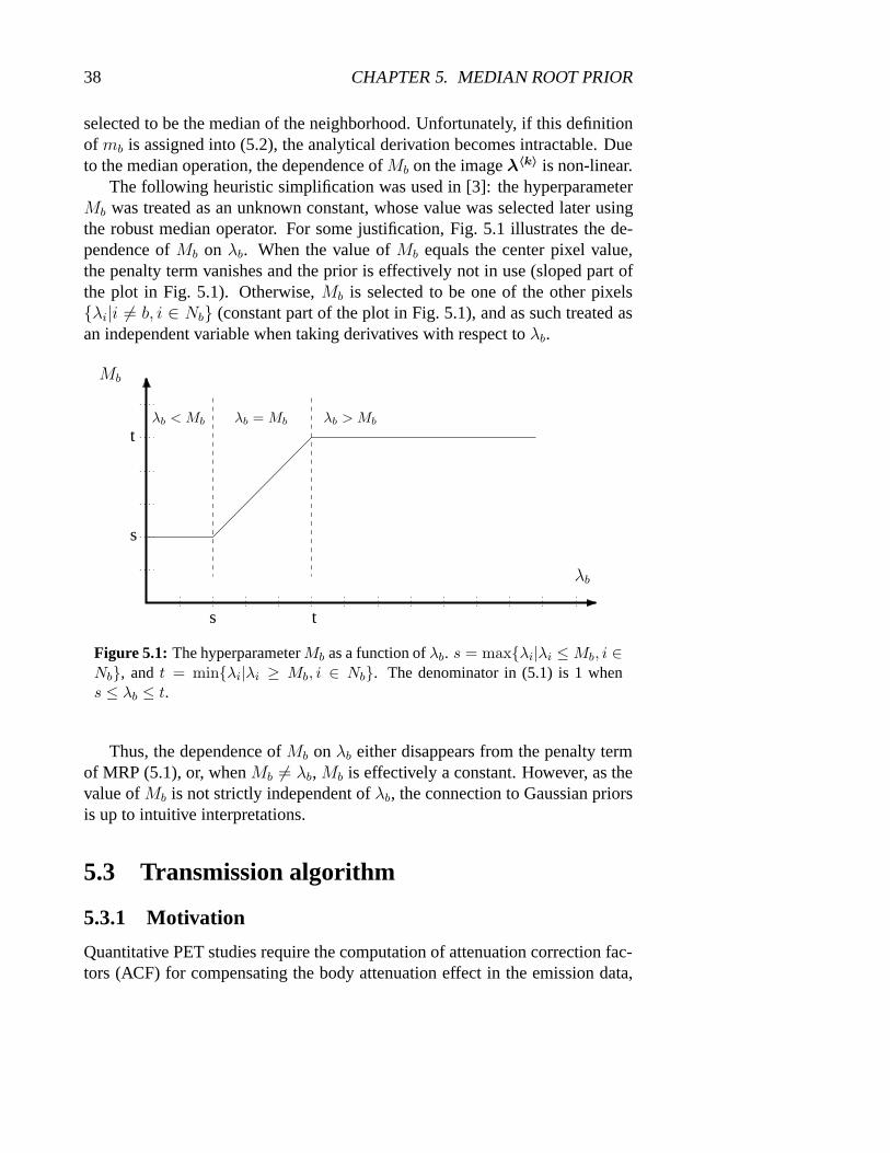
The following heuristic simplification was used in [3]: the hyperparameterMb was treated as an unknown constant, whose value was selected later usingthe robust median operator. For some justification, Fig. 5.1 illustrates the de-pendence ofMb on λb. When the value ofMb equals the center pixel value,the penalty term vanishes and the prior is effectively not in use (sloped part ofthe plot in Fig. 5.1). Otherwise,Mb is selected to be one of the other pixels{λi|i 6= b, i ∈ Nb} (constant part of the plot in Fig. 5.1), and as such treated asan independent variable when taking derivatives with respect toλb.

ts

s

tλb < Mb λb = Mb

λb

λb > Mb

Mb

Figure 5.1: The hyperparameterMb as a function ofλb. s = max{λi|λi ≤ Mb, i ∈Nb}, andt = min{λi|λi ≥ Mb, i ∈ Nb}. The denominator in (5.1) is 1 whens ≤ λb ≤ t.

Thus, the dependence ofMb on λb either disappears from the penalty termof MRP (5.1), or, whenMb 6= λb, Mb is effectively a constant. However, as thevalue ofMb is not strictly independent ofλb, the connection to Gaussian priorsis up to intuitive interpretations.

5.3 Transmission algorithm

5.3.1 Motivation

Quantitative PET studies require the computation of attenuation correction fac-tors (ACF) for compensating the body attenuation effect in the emission data,

5.3. TRANSMISSION ALGORITHM 39

as mentioned in Section 2.2.1. When emission data are multiplied by the ACFs,the noise or blurring caused by smoothing propagate from ACFs to the emissiondata.

If the image of linear mass absorption coefficientsµ is available, the ACFscan be generated by implementing the principle of Eq. (2.3). From the recon-structedµ-image, the ACFs are computed as

ACF d = eR(ld, µ) , (5.8)

whereR(ld,µ) ,∑

b ldbµb is the forward-projection of the imageµ to the LORd, andldb is the weight of the contribution of pixelb to LORd.

As mentioned in Section 3.1.2, transmission image can be reconstructed us-ing FBP from blank and transmission measurements. However, FBP images arenoisy and some bias may introduced in the transmission image [28]. Usuallythe image is segmented before (5.8) in order to reduce noise and artifacts. Thismeans that some assumptions need to be made about tissue types and their typ-ical µ-values [63, 84]. The segmentation method is rather complex to apply fora diverse set of attenuation values. In practice, some details may not properlycontribute to the ACFs [77]. Thus, high quality transmission images are desiredfor accurate attenuation correction.

5.3.2 Data fitting algorithm

The iterative methods do not usually reconstruct the logarithm of the ACFs(2.2), but use a more precise statistical model for the scans [30]. The likelihoodfor the measured transmission data is Poisson

f(T | µ) =∏

d

e−Bd e−R(ld,µ)

(Bd e−R(ld,µ)

)Td

Td!, (5.9)

whereB is the blank sinogram, andT is the transmission sinogram.µb is theprobability of photon capture per unit length for pixelb. The mean of the Pois-son can include random eventsrd such as accidentals or scatter:Bd e−R(ld,µ) +rd, if available [28].

The objective function to be maximized is the log-likelihood

L(µ) =∑

d

[−Bd e−R(ld,µ) − Td R(ld,µ)]+ C . (5.10)

The MLEM algorithm for (5.10) was developed in [58] using a complete dataformulation, but it is too slow in practice [59]. The convex algorithm for trans-mission by Lange et al. [59] is commonly used instead. It uses Newton’s itera-tion and updates the pixel as


µC〈k+1〉b = µ

〈k〉b +

µ〈k〉b

∑d ldb[Bd e−R(ld,µ〈k〉) − Td]∑

d ldb R(ld,µ〈k〉) Bd e−R(ld,µ〈k〉). (5.11)

If B andT have different acquisition times,B is scaled accordingly.B andT are both normalized for detector compensation. There are various ways toinclude mathematical priors of the type of Table 3.2 into (5.11) [59]. Anatomi-cal priors are not an option because a CT or MRI image could be used in placeof the ET transmission image. The OS acceleration method (Section 3.5.1) canbe applied for the convex algorithm [46].

5.3.3 tMRP algorithm

The algorithm (5.11) is ill-posed and some regularization is required. Becausethe assumption of local monotonicity of the true image is equally valid for bothemission and transmission, MRP can be used as the penalty. The aim is to tomake high quality transmission images with as short transmission acquisitiontimes as possible. These images are used in computing low noise ACFs foremission data.

MRP can be applied to (5.11) analogously to the emission OSL algorithm(5.1). The transmission image is computed by the tMRP (transmission MRP)algorithm [6, 5]

µ〈k+1〉b =

1

1 + βµ〈k〉b −Mb

Mb

µC〈k+1〉b , (5.12)

whereµ〈k〉 is the current transmission image, andMb = Med{µ〈k〉i |i ∈ Nb}.

The role of the parameterβ is the same as for the emission OSL-algorithm.(5.12) is simplest way to apply the penalty of MRP to any transmission

algorithm. The convex transmission algorithm (5.11) is relatively slow due tothe exponentiations. There are other transmission algorithms [28, 30], and theirspeed depends on the update strategy of the algorithm, as discussed in Section3.5.1.

With tMRP, the ACFs can be generated from count-limited data with poorstatistics without smoothing or segmentation, and no assumptions need to bemade about tissue types and typicalµ-values. tMRP can be applied to vari-ous procedures carrying out the transmission scan, such as the simultaneoustransmission-emission scan mentioned in Section 2.2.1. tMRP can also be usedfor generation of the attenuation map for the cases where attenuation is includedin the projection weighting factorspdb of the emission reconstruction algorithm.

5.4. ON CONVERGENCE PROPERTIES 41

5.4 On convergence properties

As an OSL, MRP shares with the convergence properties of an OSL algorithm[56]. The effect of the prior on the convergence of the updating algorithm can beexamined by the properties of the log-prior part of the objective function [57].The fact thatMb is nonlinearly dependent onλb, makes it not easy to rigorouslyderive the convergence properties of MRP. However, with the simplistic butintuitive interpretation of the nature of the hyperparameterMb ∈ {λi | i 6= b}(page 38 and [3]), MRP enjoys same properties that motivated the usage ofthe gamma prior (3.29, page 28) [57]. A rigorous derivation of convergenceproperties of MRP is still a challenging problem.

In the absence of a proof of the convergence of MRP, the experience of usingMRP in practice has not brought up any problems of instability. This issue willbe addressed in Section 6.1.

5.5 Noise and bias

MRP operates solely on the current image estimate computed by the updatingalgorithm (MLEM or any other one). As there are no quantitative assumptionsor thresholds in the design of the prior itself, MRP is supposed to have a verysmall bias. The noise suppression is based on a general description of anyobject, which leaves the updating algorithm the liberty to proceed with as manyiterations as is needed.

5.6 Implementation

5.6.1 Neighborhood size

The spatial size of the median mask defines the area, over which the criteriaof monotonicity is required, or in other words, the neighborhood system ofthe corresponding MRF. This gives the possibility to pre-set the width of thesmallest detail to be preserved. The width of the smallest horizontal or verticaldetail that a root signal can contain is half of the mask size

dw =(mw + 1)

2pw =

(mw + 1) fov

2 iw zoom, (5.13)

wheremw is the median mask width [pixels],pw is the pixel width [mm],fov is the width of FOV [mm],iw is the image width [pixels], andzoom =fov/(iw pw). By setting the image dimension, the zoom factor, and the masksize accordingly (so that small neighboring objects do not both fall inside the


mask), MRP penalizes only details smaller than a known size (5.13). This re-quires that the number of pixels in the image is adjusted to be large enough, sothat the mask size in pixels is reasonable (3×3 or perhaps preferably 5×5). Thesize of those small neighboring objects is easier to set beforehand than quan-titative thresholds. Thus, the mask size affects the granularity rather than theresolution or the sensitivity. Unfortunately, the computation time of the datafitting part of the algorithm increases heavily along with the image dimension.

5.6.2 Parameterβ

After choosing the neighborhood size, the weight of the prior must be cho-sen. Neither of the MRP-algorithms, emission (5.1) and transmission (5.12),have other user-set tuning parameters than the Bayes weight,β. The robust-ness of median makes the choice ofβ rather uncritical (see Section 6.1.4).Experimentally [2, 4, 3, 52, 47],β ≈ 0.3 is a good choice for (5.1) whenmw = 3. If mw = 5, there are more pixels inside the mask andβ can besmaller:β = 0.3 × 32/52 ≈ 0.11.

Greater values ofβ shift the new pixel value closer toMb setting moreweight on the assumption that the image should be locally monotonic. Thecloser the image is to its median-filtered image, the less the prior needs tochange the image. MRP does not use the median filter as a direct operation,but rather as a way to compute a reference for the penalty. As pointed out onpage 25, the smoothing prior uses a FIR filter for the penalty reference in asimilar way. On flat areas the difference between a low-pass FIR and the me-dian is quite small, especially with a larger 5×5-mask. The difference is thatthe median brings the edge preservation capability into the algorithm withouttuned hyperparameters.

5.6.3 Iterations

The iterations of MRP start with a uniform disk as an initial image. The fewfirst iterations are plain MLEM iterations. The penalty is taken in use after 2– 4 iterations. This is because during the early iterations MLEM does not yetgenerate noise to the image, but forms a coarse approximation of the image.Small details and high spatial frequencies are produced at later iterations, andthere is no need to control the monotonicity of the image right from the start.Also, the approximations made with the OSL-algorithm (page 24) are less sig-nificant at later iterations, when the changes of the pixels between the iterationsare generally small. Fig. 5.2 shows images of a MRP sequence of iterations.Compared with the MLEM sequence of Fig. 3.5 on page 22, later iterations donot generate noise in the MRP images.

5.6. IMPLEMENTATION 43

Figure 5.2: Intermediate MRP reconstructions.Top row: iterations 5, 10, 20, and30. Bottom row: iterations 40, 50, 60, and 100.

A smoothed FBP image as the first image instead of the disk might save afew iterations in the beginning. However, in order to get rid of FBP-artifacts anddevelop sharp edges, the number of iterations needs to be quite high. BecauseMRP can tolerate a high number of iterations, the initial image is not critical tothe result. Using a uniform disk as the first image is the simplest and the mostneutral choice.

Based on what was mentioned in Section 3.5.1, the OS acceleration methodcan be used with MRP with moderate number of subsets. With OS factor nomore than 4, the MRP penalty can be applied after each sub-iteration. A possi-ble way to use temporal averaging with higher OS factor is shown in Fig. 5.3.The sinogram frame is split into few (3) frames of shorter acquisition times,They are reconstructed separately with a larger OS factor (16 or 32). The sumof the sub-images averages out some of the temporal fluctuations caused bydifferent noise realizations. The common part of the sub-images represent thenon-random signal, which is preserved in the summation. As the averaging iscarried out in the temporal dimension, there seems to be hardly any spatial blur-ring. In contrast, FBP as a linear operation deals with the noise in the split andin the total sinograms the same way. This simple experiment suggests, evenwithout considering the OS-factors, that spatial fluctuations due to noise andthe ”true” image may be distinguished in the time dimension. Noise is dynamicand the spatial activity distribution is nearly static.


(a) MRP, 144 iterations, 3 sec frame.

(b) MRP, 9 iterations with OS=16, 144 total iterations, 1+1+1 sec frame.

Figure 5.3: MRP reconstructions of a 3 second frame and the sum of three 1 secondframes of the same acquisition period. The computation time is saved by the factorof 16/3 ≈ 5.

Chapter 6

Results and Images

6.1 Simulations

The effect of noise on the accuracy and the quality of the reconstructed im-ages was examined using a simulated phantom. The phantom was based onthe Shepp-Logan phantom [76]. Because a piecewise constant phantom is anunnatural object and maybe too easy for the reconstruction task, a part of thephantom image was made smooth by repetitive filtering using 5×5, 7×7, and9×9 running averages. The phantom was not meant to be the most realisticone for ET, but it serves as a basis for quantitative tests. Methodologically, thereconstruction method should be able to generate any kind of an image.

The phantom was re-projected to a noiseless sinogram. Poisson noise wasadded to it. Altogether 100 different noise realizations were generated by usinga different seed of the random number generator [71]. The deviation was in-creased by the factor of 4, 6, 8, 10, and 12 at multiples of ten during the 50 firstrealizations [72]. For the last 50 realizations, the deviation was not changed,just the seed. These sinograms were reconstructed using different algorithmsand parameters (see Table 6.1). The aim is to compare MRP with the wellknownde factostandards, FBP and MLEM. Because the various other priorsmay require careful parameter optimization and more complex implementationtechniques, they were excluded from the comparison.

In order to examine the consequences of the selection of reconstructionmethod and its parameters, the images were checked against the known truephantom image and the statistical properties of the images were examined. FourROIs were used, see Table 6.1.

45

46 CHAPTER 6. RESULTS AND IMAGES

Table 6.1: Notations used in Section 6.1.Abbreviation Explanation

FBP FBP with Hann

FBPr FBP with ramp

ML16 MLEM with 16 iterations

ML48 MLEM with 48 iterations

ML MLEM with 144 iterations

MRP1 MRP withβ = 0.1 and 144 iterations





ROI1 329 pixels of a uniform low value

ROI2 3259 pixels of a uniform medium value

ROI3 140 pixels of a uniform high value

ROI4 1960 pixels, the blurred part

6.1.1 Error histograms

Fig. 6.1 shows the histograms of the error images (the reconstructed image –the true phantom) over all 100 images for two different ROIs. The histogram ofthe error was calculated over the set{

λbi − tbtROI

100% | b ∈ ROI , ∀ i

}, (6.1)

whereb is the pixel index,i is the noise realization (sinogram or image) index(1 ≤ i ≤ I), tb is the true pixel value, andtROI is the true ROI average. Awide histogram means a large variability and weak reliability of the quantita-tive result of an individual image. A shift of the position of the peak of thehistogram away from the vertical line of zero error in Fig. 6.1 indicates a riskof a systematic bias.

Fig. 6.1(a) shows how sensitive the local bias of MLEM is to the number ofiterations and to the initial value of the image. When the number of iterationsincrease, the histogram shifts closer to the zero error position, but at the sametime it gets much wider. Interestingly, the fully converged MLEM gives a neg-ative mode for ROI1 and its distribution is roughly as wide as FBP’s. MRP’s

6.1. SIMULATIONS 47

(a) ROI1

(b) ROI4

Figure 6.1: Histograms of the error of the modified Shepp-Logan phantom recon-structions. The ROI pixels are marked black on the negative phantom images. Solidline: MRP3. Dashed: FBP. Long dashes: FBP. Dotted: ML16. Dash-dotted:ML48. Dash-dot-dot-dotted: ML. The histogram cell size is 3% for ROI1 and 1%for ROI4. The y-axis shows the probability (%) of error falling in the cell.

error histogram is both narrow and at the right position.

The non-uniform ROI4 in Fig. 6.1(b) demonstrates that also a smooth part ofthe MRP3 image is quantitatively accurate. This is because the requirement of


local monotonicity includes smoothness. ML16 produces an asymmetric errorhistogram.

For larger ROIs all methods perform quite well, but the width of the errorhistogram of ML16 and MRP3 are the two narrowest ones. With more itera-tions, MLEM is close to FBP or FBPr.

The error histograms for MRP are compact and centered around zero for allROIs. Different values ofβ are not shown for MRP because they had only asmall effect on the histograms, withβ = 0.9 slightly the most compact. On theother hand, the number of iterations used for MLEM has a strong effect both onthe shape and on the location of the error histogram, similar to the differencebetween FBP and FBPr.

6.1.2 Reliability of ROI estimation

A desirable property of a ET reconstruction method is to produce images fromwhich ROI estimates can be reliably analyzed. It is important to notice that thecommon ROI average calculation is yet another estimation task after the recon-struction task itself. A sample mean of the ROI pixels as an estimate of the trueROI value is more reliable if the values of the sample pixels form a symmetricdistribution. Even if the ROI average is expected to be unbiased, heavy tailsof an asymmetric sample distribution increase the possibility of outliers. Theoutliers affect on the sample mean of an individual realization causing potentialbias, especially for a small ROI.

One of the simplest measures of the symmetry of the distribution is theskewness [71]. Fig. 6.2 shows the average skewness values of ROI2 for eachreconstruction method. The average skewness was calculated as

skew ({λbi|b ∈ ROI, ∀ i}) =1

I

I∑i=1

[1

B

B∑b=1

(λbi − λi

σi

)3]

, (6.2)

whereλi is the ROI mean of theith image, andσi is the standard deviationof the ROI of theith image. The closer the skewness is to zero, the moresymmetrical the sample distribution is. If the skewness is not close to zero,there is a risk that the ROI average of an individual image is a biased estimatorfor the desired quantity. ML tends to produce tails to the positive direction. Interms of skewness, MRP performs well. FBP is very good, but FBP may havesome local bias (Fig. 6.4(a)).

6.1. SIMULATIONS 49

0.01

FBP

-0.00

FBPr

-0.23

ML16

0.38

ML48

0.54

ML

0.14

MRP1

0.11

MRP3

0.10

MRP5

0.10

MRP7

0.10

MRP9

Figure 6.2: The skewness values of a ROI2 averaged over all noise realizations.Skewness values close to zero indicate symmetric distributions and reliable sam-ple means. The approximate limit for significant value of the skewness [71] is3√

15/B = 0.2 .

6.1.3 Noise sensitivity

The estimators may behave in a different way when operating on noisy data.Fig. 6.3 shows MAE for each noise realization. MAE is calculated for eachimage as

MAE (i) =

∑b∈ROI |λbi − tb|BROI tROI

100% , (6.3)

wherei is the noise realization index, andBROI is the number of pixels in theROI.

In Fig. 6.3 the five different noise deviations used when generating the inputdata can be seen as an increase of MAE of MLEM at multiples of ten (i < 50).MRP3 is less sensitive to the amount of noise in the sinogram. On the otherhand, what it comes to MAE, ML serves as a noise amplifier. There are noother MRP reconstructions with differentβ values plotted in Fig. 6.3 becausethey are almost indistinguishable from each others. Because the positive andnegative errors do not cancel out in MAE, a small MAE value indicates thatalso the smooth part of the phantom is accurately reconstructed by MRP.

6.1.4 Parameter sensitivity

Fig. 6.4 shows the robustness of the behavior of the reconstruction method. Thefigures of merit are calculated for each method as

bias =

∑b∈ROI (λb − tb)

BROI tROI

100% , (6.4)

efficiency =σ2

FBP

σ2, (6.5)


Figure 6.3: The average (%) of MAE of ROI4 for each noise realization. Solidlines: MRP3. Dashed: FBP. Dotted: ML16. Dash-dotted: ML48. Dash-dot-dot-dotted: ML.

MSE = bias2 + σ2 , (6.6)

and

MAE =

∑b∈ROI |λb − tb|BROI tROI

100% , (6.7)

whereλb = (∑

i λbi)/I is the sample mean of reconstructed pixels atb in the setof I images, andσ2 = Var(λbi) is the variance ofIBROI reconstructed pixels.

In Fig. 6.4(a), the bias is the smallest for MRP, and differentβ values ofMRP make a very small difference. The amount of bias introduced by using alimited number of iterations for MLEM depended on the chosen ROI.

Fig. 6.4(b) depicts the variability of the estimate in terms of the relativeefficiency (6.5) compared to FBP. The relative efficiency should be more than1 in order to perform better than FBP in noise reduction. Only ML16 and MRPwith β > 0.1 achieve this. The price paid for the excellent efficiency of ML16is the bias.

In Fig. 6.4(c) MSE is shown. MSE takes both the bias and the varianceinto account, but the bias is so small that the variance is the dominating part.ML16 performs well, but with full number of iterations ML has almost as largeMSE as FBPr. Again, MRP performs equally well independently ofβ. FBP

6.1. SIMULATIONS 51

0

-2

-1.26

FBP

-1.16

FBPr

-1.08

ML16

-0.39

ML48

-0.16

ML

-0.11

MRP1

-0.09

MRP3

-0.08

MRP5

-0.07

MRP7

-0.07

MRP9

(a) Bias (%) of ROI4 average

0

4

0.14

FBPr

3.29

ML16

0.66

ML48

0.20

ML

1.03

MRP1

1.43

MRP3

1.55

MRP5

1.60

MRP7

1.63

MRP9

(b) Relative efficiency with respect to FBP

0

2

0.28

FBP

1.86

FBPr

0.09

ML16

0.42

ML48

1.38

ML

0.37

MRP1

0.32

MRP3

0.31

MRP5

0.31

MRP7

0.30

MRP9

(c) MSE (%) of ROI4 average

0

3

1.37

FBP

2.64

FBPr

1.45

ML16

0.59

ML48

1.77

ML

0.33

MRP1

0.25

MRP3

0.23

MRP5

0.22

MRP7

0.21

MRP9

(d) MSE (%) of ROI3 average

0

8

1.90

FBP

3.64

FBPr

7.17

ML16

2.83

ML48

3.57

ML

1.54

MRP1

1.41

MRP3

1.41

MRP5

1.41

MRP7

1.41

MRP9

(e) MAE (%) of ROI4 average

Figure 6.4: Bias, MSE, the relative efficiency, and MAE of each reconstructionmethod calculated for a ROI. MRP is robust with respect toβ.

performs remarkably well. The change of ROI4 to ROI3 in Fig. 6.4(d) worsensFBP and ML16. Thus, the optimal number of iterations for MLEM depends on


the chosen ROI.Fig. 6.4(e) shows how MAE ranks the methods. Although 6.4(e) and 6.4(c)

are computed for the same ROI, the choice of the figure of merit (MSE or MAE)gives different results regarding the optimal number of iterations for MLEM.MRP is more consistent in this sense.

6.1.5 Images

Fig. 6.5 shows images of the phantom study. The first and the second row showthe reconstructed images, with a small and a large amount of noise, respectively.ML48 is close to FBP, and ML is close to FBPr. This suggest that the numberof iterations as a global regularization method suffers from the same kind oftrade-off as FBP’s filter functions.

Figure 6.5: Phantom images. From left to right: FBP, FBPr, ML16, ML48, ML,and MRP3. 1st row: reconstructed images with the smallest amount of noise inthe sinogram.2nd row: reconstructed images with the largest amount of noise inthe sinogram.3rd row : average bias images. Pixels with an error larger (smaller)than 10% of the low activity of ROI1 are marked white (black).4th row: averagepixel-wise standard deviation. Images on each row are scaled for display using thesame factor.

On the third row there are the average bias images computed for each pixelwith respect to all 100 reconstructions of the noise realizations

6.2. CLINICAL DATA 53

bias(b) =

∑i(λbi − tb)

I. (6.8)

Bias values greater than 10% of the activity of ROI1 are marked with white pix-els, and negative bias values of the same amount are marked black. Thus, largewhite or black areas (ML16) are undesirable because they suggest that the pixelvalues of an individual image may be systematically biased. On the other hand,areas with mixed white and black pixels (ML, FBPr) may be quantitatively ac-curate on the average across different noise realizations, but the ROI value ofan individual image may be sensitive to noise.

The fourth row of Fig. 6.5 shows the pixel-wise standard deviation imagescomputed with respect to the noise realizations,

√Var(λb). ML seems to have

a strong data-dependent variance, which makes areas with a high activity quitenoisy. MRP3 expresses some edge jitter [10].

The MRP3 images on the rightmost column show some desirable proper-ties. There are no large areas with a systematic bias, and the variability of theestimate is small in general. The MRP images itself may look unconventional,especially if the sinogram is very noisy. But the quantitative properties shouldoverweight the pleasing of the human eye.

6.2 Clinical data

Clinical PET data acquired using ECAT931/08-12 (CTI/Siemens, Knoxville,USA) were reconstructed using MRP (5.1). More clinical images are shown inthe publications II – IV.

6.2.1 Emission studies

Fig. 6.6 shows reconstructions of the same study as Fig. 3.3 on page 15. Com-pared to FBP, the iterative methods do not spread out strong artifacts due to thehigh activity in the vein. OS factor 4 was used for both MLEM and MRP. Thedifference between the images in Fig. 6.6 is that the early stoppage of MLEMhas performed some global noise reduction, whereas MRP does it locally.

By increasing the dimensions of both the median mask and the image, thespatial size of the mask can be kept the same. Then there are more pixels in theset from which the local median is selected and the appearance of the image isless blocky. Fig. 6.7 shows an MRP image with the mask size increased from3×3 to 5×5 mask and image dimension from 128 to128 × 5/3 ≈ 212. Thecomputation time increases along with the size of the image.

The general form of MRP allows its usage for any organ and for any traceruptake. In order to illustrate that, Figs. 6.8 and 6.9 show images of legs and


Figure 6.6: PET FDG images. Image dimension = 128.Left : MLEM, 5 iterationswith OS=4, 20 total iterations.Right: MRP withβ = 0.3, 3×3 mask, 36 iterationswith OS = 4, 144 total iterations. High activity in the vein does not contribute toother parts of the image. The early stoppage of MLEM may have caused somenoise / bias trade-off.

Figure 6.7: MRP with β = 0.11, mask size 5×5 and image dimension 212, 36iterations with OS = 4, 144 total iterations. The mask size is spatially the same (1.4cm) as for the MRP image in Fig. 6.6.

the brain, respectively. The difference imagesA − B in Fig. 6.8 show excessin A as white pixels and excess inB as black pixels. The difference imagesshow how noise artifacts in the FBP image are removed from the MRP image.MLEM with only a few iterations is not yet very noisy, but the quantitative levelin the bone is too high [3].

One of the simplest edge detection operations, Sobel [40], was used in Fig.6.9 for emphasizing that MRP effectively removes noise without blurring theimage. FBP and aborted MLEM do not produce sharp edges where there should

6.2. CLINICAL DATA 55

Figure 6.8: PET FDG thigh images.Left : Difference image FBP (Hann) – MRP.Middle : Difference image MLEM (5 iterations with OS=4, 20 total iterations) –MRP. Right: MRP with β = 0.3, 3×3 mask, 36 iterations with OS = 4, 144 totaliterations. Image dimension = 128.

Figure 6.9: Sobel edges of PET FDG brain images. Image dimension = 128. Fromleft to right: FBP; MLEM, 5 iterations with OS=4, 20 total iterations; MLEM, 36iterations with OS = 4, 144 total iterations; and MRP with 3×3 mask, 36 iterationswith OS = 4.

be. Converged MLEM is notoriously noisy, whereas MRP is sharp and ex-presses a low amount of noise. The good separability of tissue borders facili-tates the drawing of ROIs. However, it is noteworthy that there are also low andsmooth transitions between different concentration levels. The MRP image assuch seems to be suitable for various post-reconstruction operations.

6.2.2 Transmission

The motivation for using tMRP (5.12) for transmission image reconstruction isto avoid the count-limited noise from occuring in the image and, consequently,in the ACFs. Fig. 6.10 shows ACFs computed by the conventional method witha long scan time and by using tMRP with the short time. In spite of the increasedcount-limited noise in the latter, the ACFs are as good as, if not better than in theconventional case. This was accomplished without any object dependent post-reconstruction operations such as the segmentation of the transmission image


and the tissue type classification [63, 13, 77, 84].

Figure 6.10: PET ACFs. Left : conventional, 20 min scan time.Right: ACFscomputed using tMRP withβ = 0.5, 5×5 mask, 100 iterations, 2 min scan time.The contour lines are drawn at ACF values of 2, 4, 8, and 16.

More results and tMRP transmission images are presented in publication IV[5].

6.2.3 Whole body studies

A single set of acquired sinogram planes covers only 10 – 15 cm in the axial di-rection. Whole body studies are commonly done without attenuation correctionbecause multiple transmission scans at different axial positions take too muchtime using the conventional method. The possibility to use short transmissionacquisition times and the absence of post-reconstruction operations make tMRPsuitable for computing the transmission images and the ACFs for a whole bodystudy. Fig. 6.11 shows coronal transmission images and attenuation correctedemission images. The transmission scan time for each axial position was 2min. Although the computation time is significantly longer than using the con-ventional method, it is more easily expandable than the scanner time for thepatient.

6.3. SPECT IMAGES 57

(a) Transmission (b) Emission

Figure 6.11: Coronal whole body PET images of a clinical study. The imagesare made by stacking transaxial images. The emission images were corrected forattenuation.

6.3 SPECT images

MRP has been applied for SPECT transmission and emission reconstruction[49]. Fig. 6.12 shows heart emission images acquired using a SPECT devicewith 64 projection angles / 360◦ (Siemens Orbiter, Siemens Medical Systems,Inc., Hoffman Estates, Il., USA). No attenuation correction was applied.

(a) FBP. (b) MRP, 70 iterations,β = 0.2, 5×5mask, image dimension 200.

Figure 6.12: SPECT images of a clinical heart study.

Siemens Multispect3 three-head gamma camera with fan-beam collimatorsand 128 projection angles / 360◦ was used for quantitative studies with mea-


sured attenuation correction. No attenuation pre-correction was applied on theemission data. Fig. 6.13 compares aborted MLEM and MRP. As in PET, MRPreduces noise without blurring details. MRP is especially suitable for the re-construction of the attenuation map, Fig. 6.13(a).

(a) Transmission.Left : MLEM, 24 iterations.Right: MRP,24 iterations,β = 0.3, 5×5 mask.

(b) Emission. Left : MLEM, 12 iterations. Right: MRP, 60iterations,β = 0.15, 5×5 mask.

Figure 6.13: SPECT images of a clinical brain study. The transmission imageswere used as the attenuation maps in the emission reconstruction. Larkin’s OSEMpackage [39] version 5 was modified for MRP.

6.4 Summary of results and the publications

A large portion of the material of the enclosed publications is rewritten for thismanuscript for the sake of clarity. However, the detailed results are not repeated

6.4. SUMMARY OF RESULTS AND THE PUBLICATIONS 59

here.Publication I [1] documents the first appearance of MRP in a scientific fo-

rum. The results were tentative but consistent with later examinations. Publi-cation II [2] included more quantitative tests of the new method presented toa wider audience. A stabile behavior with respect to iterations were demon-strated. Both a good resolution and a low noise level were possible to achieveat the same time. Publication III [3] further expands the theoretical inspectionof the prior. The interpretation for the Gaussian PDF of the prior was formu-lated. Good convergence properties as well as a small noise / bias trade-off werereported. As a possible step towards visual enhancement, a FIR-median-hybridfilter was suggested to be used instead of the standard median, if more conve-nient. Publication IV [5] extends the application of MRP to the transmissionimage reconstruction for attenuation correction. The good tolerance against thecount-limited noise made short time transmission scans possible.

The new tests in this section are to demonstrate the insensitivity of MRPagainst different noise realizations, both in terms of bias and variability of theestimate. As the simulations are free from attenuation, the effects of an impre-cise statistical model due to pre-corrections do not contribute here.

The histograms of the pixel-by-pixel errors in Section 6.1.1 showed thatMRP produces errors of moderate magnitude. According to the skewness testin Section 6.1.2, the errors form symmetric distributions. This is important inparametric images.

In [15], it is pointed out that a non-convex penalty function resulting from anon-linearity (e.g. threshold) may cause a sudden change in the estimate if theinput data is slightly varied. The results in Section 6.1.3 anecdotally indicatethat the non-linear and strictly speaking non-convex penalty function of MRPseem not to cause such sudden changes in the pixel values when the noise isvaried and increased in the sinogram.

Fig. 6.4 in Section 6.1.4 indicates that MRP is robust with respect to the se-lected value of the parameterβ. MRP performs well in terms of all four figuresof merit. Furthermore, the behavior of MRP does not significantly depend onthe chosen ROI, which reflects robustness with respect to the activity in otherparts of the image.

The different values ofβ behave in a robust way for all the tests. A moderatevalue (β ≈ 0.3) lets the image be not exactly locally monotonic, which helps indepicting local extremes in the image.

MRP performs well in light of the variability. Concerning the complexity ofmany other priors (parameter tuned, anatomical), the possible gain with respectto MRP, if any, may be too small for the extra effort.

Visually MRP images may lack of conventionally common features, suchas blurred edges. For pure visual analysis, some post-reconstruction filters may


be used, if more convenient. SPECT might be such a case.As the results in this section indicate, the MRP images share some quanti-

tatively important features: the bias and the variability of the estimate are smallat the same time, and the ROI averages are insensitive both to the input noiseand to the neighboring image structure. The results denote that it is safe to useMRP images as a basis of quantitative pixel-by-pixel or ROI analysis.

Chapter 7

Discussion

7.1 General principle

A priori is a term used to identify a type of knowledge which is obtained inde-pendently of experience. In MRP, the prior assumption is that an ideal emis-sion image is locally monotonic. Inside a neighborhood of a certain size, thereare only monotonic changes in activity between pixels. The monotonicity in-cludes sharp step edges, shallow ramp edges, and arbitrarily smooth edges ofany height. This is also the structure of a root signal of the median filter. Theroot signal is the penalty reference of MRP. Thus, MRP contains implicitly thegeneral description of the unknown tracer concentration. When the spatial sizeof the neighborhood is reasonably selected and it contains a sufficient numberof pixels, the true image is left automatically almost completely unpenalized.No special knowledge of the appearance of the true image is required. This uni-versal nature of the prior makes the definition of the penalty of MRP virtuallyindependent of the organ or the tracer.

The Bayesian interpretation of the penalty of MRP is close to an indepen-dent Gaussian prior PDF for the mean activity of the pixel. The location of theheuristic PDF is the median of the neighborhood. Thus, the general descriptionof the true image is modeled using a Markov random field, where the spatialdependence of the pixels is accomplished only by the median. This makes un-known differences between the pixel values permitted in the prior model ofMRP.

The problem with mathematical priors is to describe the properties of thetrue image as a function of the pixel differences in the neighborhood. Thequadratic energy function results in a penalty with respect to the difference be-tween the center pixel and the weighted average. The operation is similar to alowpass filter. As the frequency contents of noise and the true image overlap,a compromise between noise rejection and edge blurring must be done. The

61

62 CHAPTER 7. DISCUSSION

assumption that the unwanted roughness of the image can be expressed using alinear function of adjacent pixel differences is a restriction rather than a gener-alization.

Other choices for the energy function with tuning parameters are justifiedin terms of the behavior of the penalty in the vicinity of an edge, but the cor-responding Bayesian prior and the MRF are set up in quantitative terms: onlycertain kind of pixel differences are allowed in the neighborhood. This resultsin an almost certain penalty to the unknown true image. The resulting imagemay be a good representative for anensembleof images similar to the true im-age. But in tomography the key question is ”what is the unknown source thatgave rise to theparticular set of measurements we have?”. An average of allplausible images may not be an answer to that question.

Priors that apply penalties based on an anatomical image of the target (brain)are more specific to the given task; they rely on the assumption that the trueemission imageusuallyresembles the given anatomical image in terms of localhomogeneity. This may require further assumptions about the tissue types andtheir normalbehavior. This, in effect, may result in another good answer to awrong question.

Multimodal images are important as they reveal relations between variousimaging modalities, but with MRP the regularization of the reconstruction pro-cess itself can be left ”clean” of external data. Then the combination of the twomodalities after reconstruction is most informative. From the Bayesian point ofview, calling anatomical images as priors is somewhat artificial. That is, thereare two sets of measured data, one type of anatomical (CT, or MRI with protondensity T1 or T2 [45]) and functional (PET). Using one as a constraint when re-constructing the other might be effective technically in terms of noise reduction,but a Bayes prior should express more fundamental nature of the properties ofthe image.

The distribution for the mean tracer concentration in a pixel can be inter-preted to resemble Gaussian for MRP. The Gaussian or normal distribution isusually considered as the most cautious one when there is no other informa-tion. What is more, the central limit theorem suggests that under the influenceof many small and unrelated random effects the overall distribution is Gaussian[27, 24, 33]. Despite the fact that the connection between MRP and a Gaussianprior is more intuitive than strictly rigorous, it gives some insight into otherwiseanalytically intractable MRP algorithm. Taking the location of the Gaussian asthe median of neighboring means brings the spatial dependency in a simple,general and robust form into the algorithm.

7.2. APPLICABILITY OF MRP 63

7.2 Applicability of MRP

MRP has been applied to many clinical studies [44, 81, 73, 49, 47, 53, 54, 50].The applicability of MRP is good because the prior is very general and simple,applying for both PET and SPECT. MRP is also used in [52, 75].

In contrast to the non-Bayesian ways to control the noise, such as Hannwindow in FBP or the stoppage of iterations in MLEM, a Bayes prior dealsmore with specific local properties. The two other methods restrict the noisemore globally, which is suboptimal in local terms. A Bayes prior reflects thespatially limited range of the underlying MRF. The reconstructed image issubject to local ROI analysis, and it is important that local characteristics arenot affected by global noise reduction. MRP is especially independent of globalor external assumptions and parameters. The bias towards the initial image iseffectively avoided when MRP is used because the number of iterations can behigh enough. The results in Section 6.1 demonstrate that MRP is able to reducenoise and maintain the quantitative accuracy at the same time.

Concerning the practical usability, it is important that the method is not toosensitive to suboptimal choices of parameter values. The parameterβ of MRPis the weight of the prior, which controls the strength of monotonicity. Thevalue of the parameter is rather uncritical, which makes MRP easy to use forany study. MRP behaves consistently independently of the chosen ROI, thetracer uptake, or the tissue type.

The quantitative sensitivity of MRP is not compromised by the applied noisereduction because differences in activity with sufficient spatial size are pre-served independently of the type of the spatial transition from one activity levelto other. This size is an object dependent factor, but it can be selected beforethe reconstruction according to Eq. (5.13).

For the transmission, the aim was to compute the ACFs directly from thecount-limited transmission image reconstructed using tMRP, without any post-reconstruction steps, such as tissue segmentation. The usage of tMRP is straight-forward and simple. The principle of local monotonicity is especially suitablefor transmission images.

The parametric images are especially sensitive to pixel-by-pixel noise. MRPcan be used in reconstructing the whole sequence. Optionally, the parametricmapping can be done before the reconstruction [73]. In that case, the statisticalmodel used in the objective function should be carefully chosen, but the gen-eral principle of MRP serves for the regularization of the reconstruction of theparametric sinogram as well.

64 CHAPTER 7. DISCUSSION

7.3 Conclusion

The main strength of MRP is its simplicity. A generally accepted principle inscience is the Occam’s razor (or Ockham), which states that entities must notbe multiplied beyond what is necessary, that is, the simplest model with fewestnumber of assumptions is the one that should be selected [22]. In terms ofquality and usability, MRP is very competitive. As a comment to [2], Ph.D.I.G. Zubal writes [86]:

I am convinced that as iterative (and Bayesian) reconstruction tech-niques become more popular in nuclear medicine, we will need toslowly adjust to a new ”class” of images. The reconstruction hereshown ... [Fig. 5A in publication II], has a different quality than weare used to seeing in filtered backprojection images. This image,however, is probably a better representation of the true distributionof radioactivity within the patient. We thank the speed of modernday computers for making such improved images possible.

As pointed out by Dr. Zubal, the professionals working with ET images areused to analyze mostly smooth or noisy images. While MRP images expressthe absence of both noise and blur, they may be visually unlike what is con-ventionally considered as pleasing to the human eye. The visual aspects can beemphasized with MRP by choosing the image grid density and the mask widthcarefully, or using a FIR median hybrid in place of the median [3]. However,the modifications of the basic idea of MRP open up a large variety of median-related operations [10], which might be unnecessary. Although the visual as-pects are important, they may often reflect individual tastes, which makes itdifficult to define a visually good image in general. The quantitative merits ofMRP should not be sacrificed for the sake of subjective visual customs.

In spite of the convenient simplicity of MRP, more theoretical analysis ofthe algorithm still remains an open and challenging problem.

Bibliography

[1] S. Alenius. Bayesian image reconstruction in positron emission tomogra-phy using median root prior. InThe Proceedings of the First TUT Sym-posium on Signal Processing, pages 113–116, Tampere, Finland, May 201994.

[2] S. Alenius and U. Ruotsalainen. Bayesian image reconstruction for emis-sion tomography based on median root prior.European Journal of Nu-clear Medicine, 24(3):258–265, Mar. 1997.

[3] S. Alenius, U. Ruotsalainen, and J. Astola. Using local median as thelocation of the prior distribution in iterative emission tomography imagereconstruction.IEEE Transactions on Nuclear Science, 45(6):3097–3104,Dec. 1998.

[4] S. Alenius, U. Ruotsalainen, and J. Astola. Using local median as thelocation of the prior distribution in iterative emission tomography imagereconstruction. In1997 IEEE Medical Imaging Conference, ConferenceRecord, pages 1726–1730, 1998.

[5] S. Alenius, U. Ruotsalainen, and J. Astola. Attenuation correction for PETusing count-limited transmission images reconstructed with median rootprior. IEEE Transactions on Nuclear Science, 46(3):646–651, June 1999.

[6] S. Alenius, U. Ruotsalainen, and J. Astola. Transmission images and at-tenuation correction with short acquisitions using median root prior recon-struction in PET. In1998 IEEE Medical Imaging Conference, ConferenceRecord, pages 1711–1715, 1999.

[7] M. Alonso and E. Finn. Fundamental University Physics, volumeIII Quantum and Statistical Physics. Addison-Wesley, Reading, Mas-sachusetts, 1983.

[8] B. Ardekani, M. Braun, and B. Hutton. Improved quantification with theuse of anatomical information in PET image reconstruction. In K. Uemura

65

66 BIBLIOGRAPHY

et al., editors,Quantification of Brain Function, pages 351–359. ElsevierScience Publishers, Amsterdam, 1993.

[9] B. Ardekani, M. Braun, B. Hutton, I. Kanno, and H. Iida. A fully auto-matic multimodality image registration algorithm.Journal of ComputerAssisted Tomography, 19(4):615–623, July/August 1995.

[10] J. Astola and P. Kuosmanen.Fundamentals of nonlinear digital filtering.CRC Press, Boca Raton, 1997.

[11] D. Bailey. Transmission scanning in emission tomography.EuropeanJournal of Nuclear Medicine, 25(7):774–787, July 1998.

[12] T. Barker and J. Young. The QUT digital anatomy lab, Queensland uni-versity of technology, Australia. http://www.dal.qut.edu.au/,c©1996.

[13] V. Bettinardi, M. Gilardi, S. Cargnel, G. Rizzo, M. Teras, and G. Striano.A hybrid method of attenuation correction for positron emission tomogra-phy brain studies.European Journal of Nuclear Medicine, 21(12):1279–1284, Dec. 1994.

[14] J. Biemond, R. Lagendijk, and R. Mersereau. Iterative methods for imagedeblurring.Proceedings of the IEEE, 78(5):856–883, May 1990.

[15] C. Bouman and K. Sauer. A generalized Gaussian image model for edge-preserving MAP estimation.IEEE Transactions on Image Processing,2(3):296–310, July 1993.

[16] C. Bouman and K. Sauer. A unified approach to statistical tomographyusing coordinate descent optimization.IEEE Transactions on Image Pro-cessing, 5(3):480–492, Mar. 1996.

[17] J. Bowsher, V. Johnson, T. Turkington, R. Jaszczak, C. Floyd, and R. E.Coleman. Bayesian reconstruction and use of anatomical a priori informa-tion for emission tomography.IEEE Transactions on Medical Imaging,15(5), Oct. 1996.

[18] C. Byrne. Iterative image reconstruction algorithms based on cross-entropy minimization.IEEE Transactions on Image Processing, 2(1):96–103, Jan. 1993.

[19] A. Chatziioannou and M. Dahlbom. Detailed investigation of transmissionand emission data smoothing protocols and their effects on emission im-ages.IEEE Transactions on Nuclear Science, 43(1):290–294, Feb. 1996.

http://www.dal.qut.edu.au/

BIBLIOGRAPHY 67

[20] C. Chen, V. Johnson, W. Wong, X. Hu, and C. Metz. Bayesian imagereconstruction in positron emission tomography.IEEE Transactions onNuclear Science, 37(2):636–641, Apr. 1990.

[21] C. Comtat, P. Kinahan, J. Fessler, T. Beyer, D. Townsend, M. Defrise,and C. Michel. Reconstruction of 3D whole-body PET data using blurredanatomical labels. In1998 IEEE Medical Imaging Conference, Confer-ence Record, pages 1651–1655, 1999.

[22] F. Copleston. A History of Philosophy, volume III Ockham to Suarez.Burns and Oates Ltd, London, 1968.

[23] A. De Pierro. A modified expectation maximization algorithm for penal-ized likelihood estimation in emission tomography.IEEE Transactions onMedical Imaging, 14(1):132–137, Mar. 1995.

[24] C. Derman, L. J. Gleser, and I. Olkin.A Guide to Probability Theory andApplication. Holt, Rinehart and Winston, Inc., New York, 1973.

[25] M. Dwass. Probability and Statistics. W.A. Benjamin, Inc., New York,1970.

[26] T. Farquhar, A. Chatziioannou, G. Chinn, M. Dahlbom, and E. Hoff-man. An investigation of filter choice for filtered back-projection in PET.In 1997 IEEE Medical Imaging Conference, Conference Record, pages1042–1047, 1998.

[27] W. Feller. An Introduction to Probability Theory and Its Applications,volume I. Wiley & Sons, Inc., New York, 2nd edition, 1957.

[28] J. Fessler. Hybrid Poisson/polynomial objective functions for tomo-graphic image reconstruction from transmission scans.IEEE Transactionson Image Processing, 4(10):1439–1450, Oct. 1995.

[29] J. Fessler and N. Clinthorne.Statistical Methods for Image Reconstruc-tion and Medical Imaging System Design. 1998 IEEE NSS-MIC tutorialcourse, Nov. 10 1998.

[30] J. Fessler, E. Ficaro, N. Clinthorne, and K. Lange. Grouped-coordinateascent algorithms for penalized-likelihood transmission image reconstruc-tion. IEEE Transactions on Medical Imaging, 16(2):166–175, Apr. 1997.

[31] J. Fessler and A. Hero. Space-alternating generalized expectation-maximization algorithm. IEEE Transactions on Signal Processing,42(10):2664–2677, Oct. 1994.

68 BIBLIOGRAPHY

[32] S. Geman and D. Geman. Stochastic relaxation, Gibbs distributions, andthe Bayesian restoration of images.IEEE Transactions on Pattern Analy-sis and Machine Intelligence, 6(6):721–741, Nov. 1984.

[33] L. Gonick and W. Smith.The Cartoon Guide to Statistics. HarperCollinsPublishers, Inc., New York, 1993.

[34] P. Green. Bayesian reconstructions from emission tomography data usinga modified EM algorithm.IEEE Transactions on Medical Imaging, 9:84–93, Mar. 1990.

[35] T. Hebert and R. Leahy. A generalized EM algorithm for 3D-Bayesianreconstruction from Poisson data using Gibbs priors.IEEE Transactionson Medical Imaging, 8(2):194–202, June 1989.

[36] G. Herman.Image Reconstruction from Projections: Implementation andApplications. Springer-Verlag, Berlin, 1979.

[37] G. Herman.Image Reconstruction from Projections: The Fundamentalsof Computerized Tomography. Academic Press, New York, 1980.

[38] G. Herman and D. Odhner. Performance evaluation of an iterative imagereconstruction algorithm for positron emission tomography.IEEE Trans-actions on Medical Imaging, 10(3):336–346, Sept. 1991.

[39] H. Hudson and R. Larkin. Accelerated image reconstruction using or-dered subsets of projection data.IEEE Transactions on Medical Imaging,13(4):601–609, Dec. 1994.

[40] A. Jain. Fundamentals of Digital Image Processing. Prentice-Hall Inter-national, Englewood Cliffs, NJ, 1989.

[41] R. Jaszczak and E. Hoffman. Scatter and attenuation. In H. Wagner, edi-tor, Principles of Nuclear Medicine, chapter 19, section 3. W.B. SaundersCompany, Philadelphia, 2nd edition, 1995.

[42] R. Jaszczak and B. Tsui. General principles. In H. Wagner, editor,Princi-ples of Nuclear Medicine, chapter 18, section 1. W.B. Saunders Company,Philadelphia, 2nd edition, 1995.

[43] K. Johnson and J. Becker. The whole brain atlas.http://www.med.harvard.edu/AANLIB/home.html,c©1995-1997.

http://www.med.harvard.edu/AANLIB/home.html

BIBLIOGRAPHY 69

[44] M. Kahkonen, S. Alenius, V. Oikonen, and U. Ruotsalainen. Improvedquantitative images produced by sinogram Patlak and a new iterative re-construction method.Proceedings of the 44th Annual Meeting (San An-tonio, USA, June 1-5, 1997), the Society of Nuclear Medicine, Journal ofNuclear Medicine (suppl), 38(5):196, 1997.

[45] A. Kak and M. Slaney.Principles of Computerized Tomographic Imaging.IEEE Press, New York, 1988.

[46] C. Kamphuis and F. Beekman. Accelerated iterative transmission CT re-construction using an ordered subsets convex algorithm.IEEE Transac-tions on Medical Imaging, 17(6):1101–1105, Dec. 1998.

[47] C. Katoh, U. Ruotsalainen, H. Laine, S. Alenius, H. Iida, P. Nuutila, andJ. Knuuti. Iterative reconstruction based on median root prior in quan-tification of myocardial blood flow and oxygen metabolism.Journal ofNuclear Medicine, 40(5):862–7, 1999.

[48] L. Kaufman. Maximum likelihood, least squares, and penalized leastsquares for PET.IEEE Transactions on Medical Imaging, 12(2):200–214,June 1993.

[49] T. Kauppinen. Comparison between iteration and back-projection basedon emission tomography reconstruction methods. Lic.Sc. Thesis (inFinnish), Tampere University of Technology, Tampere, Finland, 1997.

[50] T. Kauppinen, S. Alenius, V. Turjanmaa, J. Kuikka, and M. Koski-nen. Comparison between iterative median root prior algorithm and fil-tered back-projection in SPET.European Journal of Nuclear Medicine,25(8):948, 1998. European Association of Nuclear Medicine (EANM)1998 abstract.

[51] S. Kay. Fundamentals of Statistical Signal Processing: Estimation The-ory. Prentice-Hall International, Englewood Cliffs, NJ, 1993.

[52] G. Kontaxakis, L. Strauss, and G. van Kaick. Optimized image reconstruc-tion for emission tomography using ordered subsets, median root prior,successive substitutions and a web-based interface. In1998 IEEE Medi-cal Imaging Conference, Conference Record, pages 1347–1352, 1999.

[53] H. Laine, M. Knuuti, U. Ruotsalainen, T. Utriainen, V. Oikonen,M. Raitakari, M. Luotolahti, O. Kirvela, P. Vicini, C. Cobelli, P. Nuutila,and H. Yki-Jarvinen. Preserved relative dispersion but blunted stimulationof mean flow, absolute dispersion, and blood volume by insulin in skeletal

70 BIBLIOGRAPHY

muscle of patients with essential hypertension.Circulation, 97(21):2146–53, June 1998.

[54] H. Laine, M. Luotolahti, M. Knuuti, M. Raitakari, U. Ruotsalainen,H. Iida, J. Kapanen, O. Kirvela, M. Haaparanta, H. Yki-Jarvinen, andP. Nuutila. Insulin resistance in essential hypertension is characterized byimpaired insulin stimulation of blood flow in skeletal muscle.Journal ofHypertension, 16(2):211–219, Feb. 1998.

[55] D. Lalush and B. Tsui. Attenuation and detector response compensationsused with Gibbs priors distributions for maximum a posteriori SPECTreconstruction.IEEE Transactions on Nuclear Science, 39(5):1454–1459,Oct. 1992.

[56] K. Lange. Convergence of EM image reconstruction algorithms withGibbs smoothing.IEEE Transactions on Medical Imaging, 9(4):439–446,Dec. 1990. Corrections ITMI 10(2) 1991 p. 228.

[57] K. Lange, M. Bahn, and R. Little. A theoretical study of some maximumlikelihood algorithms for emission and transmission tomography.IEEETransactions on Medical Imaging, 6(2):106–114, June 1987.

[58] K. Lange and R. Carson. EM reconstruction algorithms for emission andtransmission tomography.Journal of Computer Assisted Tomography,8(2):306–316, Apr. 1984.

[59] K. Lange and J. Fessler. Globally convergent algorithms for maximuma posteriori transmission tomography.IEEE Transactions on Image Pro-cessing, 4:1430–1438, Oct. 1995.

[60] R. Lewitt. Reconstruction algorithms: Transform methods.Proceedingsof the IEEE, 71(3):390–408, Mar. 1983.

[61] B. Lipinski, H. Herzog, R. Kops, W. Oberschelp, and H. Muller-Gartner.Expectation maximization reconstruction of positron emission tomogra-phy images using anatomical magnetic resonance information.IEEETransactions on Medical Imaging, 16:129–136, Apr. 1997.

[62] J. Llacer, E. Veklerov, K. Coakley, E. Hoffman, and J. Nunez. Statisticalanalysis of maximum likelihood estimator images of human brain FDGPET studies. IEEE Transactions on Medical Imaging, 12(2):215–231,June 1993.

BIBLIOGRAPHY 71

[63] S. Meikle, M. Dahlbom, and S. Cherry. Attenuation correction usingcount-limited transmission data in positron emission tomography.Journalof Nuclear Medicine, 34(1):143–150, Jan. 1993.

[64] Merriam-Webster Incorporated. WWWebster dictionary.http://www.m-w.com/,c©1996.

[65] C. Michel, M. Sibomana, A. Bol, X. Bernard, M. Lonneux, M. Defrise,C. Comtat, P. Kinahan, and D. Townsend. Preserving Poisson characteris-tics of PET data with weighted OSEM reconstruction. In1998 IEEE Med-ical Imaging Conference, Conference Record, pages 1323–1329, 1999.

[66] T. Moon. The expectation maximization algorithm.IEEE Signal Process-ing Magazine, pages 47–60, Nov. 1996.

[67] J. Nuyts, P. Dupont, S. Stroobants, A. Maes, L. Mortelmans, andP. Suetens. Evaluation of maximum-likelihood based attenuation correc-tion in positron emission tomography. In1998 IEEE Medical ImagingConference, Conference Record, pages 1836–1841, 1999.

[68] J. Ollinger and J. Fessler. Positron-emission tomography.IEEE SignalProcessing Magazine, pages 43–55, Jan. 1997.

[69] A. Oppenheim and R. Schafer.Discrete-Time Signal Processing. Prentice-Hall International, Englewood Cliffs, NJ, 1989.

[70] J. Pollard. Handbook of numerical & statistical techniques. CambridgeUniversity Press, Cambridge, 1977.

[71] W. Press, S. Teukolsky, W. Vetterling, and B. Flannery.Numerical Recipesin C, The Art of Scientific Computing. Cambridge University Press, Cam-bridge, second edition, 1992.

[72] R. Rowe and S. Dai. A pseudo-Poisson noise model for simulationof positron emission tomographic projection data.Medical Physics,19(4):1113–1119, Jul/Aug 1992.

[73] U. Ruotsalainen. Quantification and Data Analysis in Positron Emis-sion Tomography: Organ Blood Flow, Graphical Analysis and Radia-tion Dosimetry. PhD thesis, Tampere University of Technology, Tampere,1997.

[74] K. Sauer and C. Bouman. A local update strategy for iterative recon-struction from projections. IEEE Transactions on Signal Processing,41(2):534–548, Feb. 1993.

http://www.m-w.com/

72 BIBLIOGRAPHY

[75] A. Seret. Median root prior and ordered subsets in Bayesian image re-construction of single-photon emission tomography.European Journal ofNuclear Medicine, 25(3):215–219, Mar. 1998.

[76] L. Shepp and Y. Vardi. Maximum likelihood reconstruction for emissiontomography.IEEE Transactions on Medical Imaging, 1(2):113–122, Oct.1982.

[77] R. Smith, J. Karp, F. Benard, A. Alavi, E. Gualtieri, G. Muehllehner,and M. Geagan. A comparison of segmentation and emission subtractionfor singles transmission in PET.IEEE Transactions on Nuclear Science,45(3):1212–1218, June 1998.

[78] D. Snyder, M. Miller, L. Thomas, and D. Politte. Noise and edge artifactsin maximum likelihood reconstructions for ET.IEEE Transactions onMedical Imaging, 6(3):228–238, Sept. 1987.

[79] Sorenson. Chapter 9, Quantitative measurement of radioactivity in vivoby whole-body counting. In G. Hine and J. Sorenson, editors,Instrumen-tation in nuclear medicine, volume 2. Academic Press, New York, 1974.

[80] M. Ter-Pogossian. General principles. In H. Wagner, editor,Principles ofNuclear Medicine, chapter 19: Positron Emission Tomography, section 1.W.B. Saunders Company, Philadelphia, 2nd edition, 1995.

[81] T. Utriainen, P. Nuutila, T. Takala, P. Vicini, U. Ruotsalainen,T. Ronnemaa, T. Tolvanen, M. Raitakari, M. Haaparanta, O. Kirvela,C. Cobelli, and H. Yki-Jarvinen. Intact insulin stimulation of skeletalmuscle blood flow, its heterogeneity and redistribution, but not of glucoseuptake in non-insulin-dependent diabetes mellitus.The Journal of ClinicalInvestigation, 100(4):777–785, Aug. 1997.

[82] E. Veklerov and J. Llacer. Stopping rule for the MLE algorithm basedon statistical hypothesis testing.IEEE Transactions on Medical Imaging,6:313–319, Dec. 1987.

[83] W. Wang, C. Goldstein, and G. Gindi. Noise and resolution propertiesof gamma-penalized likelihood reconstruction. In1998 IEEE MedicalImaging Conference, Conference Record, pages 1136–1140, 1999.

[84] M. Xu, P. Cutler, and W. Luk. Adaptive, segmented attenuation correctionfor whole-body PET imaging.IEEE Transactions on Nuclear Science,43(1):331–336, Feb. 1996.

BIBLIOGRAPHY 73

[85] M. Yavuz and J. Fessler. New statistical models for randoms-precorrectedPET scans. InInformation Processing in Medical Imaging, volume 1230of Lecture Notes in Computer Science, pages 190–203. Springer Verlag,Berlin, 1997.

[86] I. Zubal. An edited abstract of [2]. In A. Gottschalk, I. Zubal, et al.,editors,1998 Year book of nuclear medicine, chapter 13, pages 416–417.Mosby Inc., St. Louis, 1998. Original paper by Alenius and Ruotsalainenselected for summary and comments.

74 BIBLIOGRAPHY

Publications

75

Publication I

S. Alenius. Bayesian Image Reconstruction in Positron Emission Tomographyusing Median Root Prior.The Proceedings of the First TUT Symposium onSignal Processing ‘94, pp. 113-116, 1994, Tampere, Finland.

Publication II

S. Alenius, U. Ruotsalainen. Bayesian image reconstruction for emission to-mography based on median root prior.European Journal of Nuclear Medicine,vol. 24, pp. 258-265, Mar 1997.

Publication III

S. Alenius, U. Ruotsalainen, J. Astola. Using local median as the location of theprior distribution in iterative emission tomography image reconstruction.IEEETransactions on Nuclear Science,selected papers from the 1997 Medical Imag-ing Conference (MIC), Albuquerque, New Mexico, November 13-15 1997, vol.45, no. 6(2), pp. 3097-3107, Dec 1998.

Publication IV

S. Alenius, U. Ruotsalainen, and J. Astola. Attenuation Correction for PETUsing Count-Limited Transmission Images Reconstructed with Median RootPrior. IEEE Transactions on Nuclear Science,selected papers from the 1998Medical Imaging Conference (MIC), Toronto, Canada, November 11-14 1998,vol. 46, no. 3(2), pp. 646-651, June 1999.

Download - ISBN 978-952-15-0279-7 (printed) ISBN 978-952-15-4216-9 (PDF)

Top Related