LEONARDO DA VINCI
Transfer of Innovation
Kristina Levišauskait÷
Investment Analysis and Portfolio Management
Leonardo da Vinci programme project
„Development and Approbation of Applied Courses Based on the Transfer of Teaching Innovations
in Finance and Management for Further Education of Entrepreneurs and Specialists in Latvia, Lithuania and Bulgaria”
Vytautas Magnus University Kaunas, Lithuania
2010
Investment Analysis and Portfolio Management
2
Table of Contents
Introduction …………………………………………………………………………...4
1. Investment environment and investment management process…………………...7
1.1 Investing versus financing……………………………………………………7
1.2. Direct versus indirect investment …………………………………………….9
1.3. Investment environment……………………………………………………..11
1.3.1. Investment vehicles …………………………………………………..11
1.3.2. Financial markets……………………………………………………...19
1.4. Investment management process…………………………………………….23
Summary…………………………………………………………………………..26
Key-terms…………………………………………………………………………28
Questions and problems…………………………………………………………...29
References and further readings…………………………………………………..30
Relevant websites…………………………………………………………………31
2. Quantitative methods of investment analysis……………………………………...32 2.1. Investment income and risk………………………………………………….32
2.1.1. Return on investment and expected rate of return…………………...32
2.1.2. Investment risk. Variance and standard deviation…………………...35
2.2. Relationship between risk and return………………………………………..36
2.2.1. Covariance……………………………………………………………36
2.2.2. Correlation and Coefficient of determination………………………...40
2.3. Relationship between the returns on stock and market portfolio……………42
2.3.1. Characteristic line and Beta factor…………………………………….43
2.3.2. Residual variance……………………………………………………...44
Summary…………………………………………………………………………...45
Key-terms………………………………………………………………………….48
Questions and problems…………………………………………………………...48
References and further readings…………………………………………………...50
3. Theory for investment portfolio formation………………………………………...51
3.1. Portfolio theory………………………………………………………………51
3.1.1. Markowitz portfolio theory…………………………………………...51
3.1.2. The expected rate of return and risk of portfolio……………………..54
3.2. Capital Asset Pricing Model…………………………………………………56
3.3. Arbitrage Price Theory………………………………………………………59
3.4. Market Efficiency Theory……………………………………………………62
Summary…………………………………………………………………………...64
Key-terms………………………………………………………………………….66
Questions and problems……………………………………………………………67
References and further readings…………………………………………………...70
4. Investment in stocks………………….....................................................................71
4.1. Stock as specific investment……………………………………………….....71
4.2. Stock analysis for investment decision making………………………………72
4.2.1. E-I-C analysis……………………………………………………….73
4.2.2. Fundamental analysis………………………………………………..75
4.3. Decision making of investment in stocks. Stock valuation…………………..77
4.4. Formation of stock portfolios………………………………………………...82
4.5. Strategies for investing in stocks……………………………………………..84
Summary…………………………………………………………………………..87
Key-terms…………………………………………………………………………90
Investment Analysis and Portfolio Management
3
Questions and problems…………………………………………………………..90
References and further readings…………………………………………………..93
Relevant websites………………………………………………………………....93
5. Investment in bonds……………………………………………………………….94
5.1. Identification and classification of bonds……………………………………94
5.2. Bond analysis: structure and contents………………………………………..98
5.2.1. Quantitative analysis…………………………………………………..98
5.2.2. Qualitative analysis…………………………………………………..101
5.2.3. Market interest rates analysis………………………………………...103
5.3. Decision making for investment in bonds. Bond valuation………………...106
5.4. Strategies for investing in bonds. Immunization…………………………...109
Summary…………………………………………………………………………113
Key-terms………………………………………………………………………..116
Questions and problems………………………………………………………….117
References and further readings………………………………………………... 118
Relevant websites………………………………………………………………..119
6. Psychological aspects in investment decision making…………………………..120
6.1. Overconfidence……………………………………………………………..120
6.2. Disposition effect…………………………………………………………...123
6.3. Perceptions of investment risk……………………………………………...124
6.4. Mental accounting and investing…………………………………………...126
6.5. Emotions and investment decisions………………………………………...128
Summary………………………………………………………………………....130
Key-terms………………………………………………………………………..132
Questions and problems………………………………………………………….132
References and further readings…………………………………………………133
7. Using options as investments……………………………………………………..135
7.1. Essentials of options………………………………………………………..135
7.2. Options pricing……………………………………………………………..136
7.3. Using options. Profit and loss on options…………………………………..138
7.4. Portfolio protection with options. Hedging………………………………...141
Summary…………………………………………………………………………143
Key-tems…………………………………………………………………………145
Questions and problems………………………………………………………….146
References and further readings…………………………………………………147
Relevant websites………………………………………………………………..147
8. Portfolio management and evaluation…………………………………………...148
8.1. Active versus passive portfolio management………………………………148
8.2. Strategic versus tactical asset allocation……………………………………150
8.3. Monitoring and revision of the portfolio…………………………………...152
8.4. Portfolio performance measures……………………………………………154
Summary…………………………………………………………………………156
Key-terms………………………………………………………………………..158
Questions and problems………………………………………………………….158
References and further readings…………………………………………………160
Relevant websites………………………………………………………………..161
Abbreviations and symbols used…………………………………………………….162
Bibliography…………………………………………………………………………164
Annexes……………………………………………………………………………...165
Investment Analysis and Portfolio Management
4
Introduction Motivation for Developing the Course
Research by the members of the project consortium Employers’ Confederation
of Latvia and Bulgarian Chamber of Commerce and Industry indicated the need for
further education courses.
Innovative Content of the Course
The course is developed to include the following innovative content:
• Key concepts of investment analysis and portfolio management which are
explained from an applied perspective emphasizing the individual
investors‘decision making issues.
• Applied exercises and problems, which cover major topics such as quantitative
methods of investment analysis and portfolio formation, stocks and bonds
analysis and valuation for investment decision making, options pricing and
using as investments, asset allocation, portfolio rebalancing, and portfolio
performance measures.
• Summaries, Key-terms, Questions and problems are provided at the end of
every chapter, which aid revision and control of knowledge acquisition during
self-study;
• References for further readings and relevant websites for broadening
knowledge and analyzing real investment environment are presented at the end
of every chapter.
Innovative Teaching Methods of the Course
The course is developed to utilize the following innovative teaching methods:
• Availability on the electronic platform with interactive learning and interactive
evaluation methods;
• Active use of case studies and participant centered learning;
• Availability in modular form;
• Utilizing two forms of learning - self-study and tutorial consultations;
• Availability in several languages simultaneously.
Target Audience for the Course
The target audience is: entrepreneurs, finance and management specialists from
Latvia, Lithuania and Bulgaria.
Investment Analysis and Portfolio Management
5
The course assumes little prior applied knowledge in the area of finance.
The course is intended for 32 academic hours (2 credit points).
Course Objectives
Investment analysis and portfolio management course objective is to help
entrepreneurs and practitioners to understand the investments field as it is currently
understood and practiced for sound investment decisions making. Following this
objective, key concepts are presented to provide an appreciation of the theory and
practice of investments, focusing on investment portfolio formation and management
issues. This course is designed to emphasize both theoretical and analytical aspects of
investment decisions and deals with modern investment theoretical concepts and
instruments. Both descriptive and quantitative materials on investing are presented.
Upon completion of this course the entrepreneurs shall be able:
• to describe and to analyze the investment environment, different types of
investment vehicles;
• to understand and to explain the logic of investment process and the
contents of its’ each stage;
• to use the quantitative methods for investment decision making – to
calculate risk and expected return of various investment tools and the
investment portfolio;
• to distinguish concepts of portfolio theory and apply its’ principals in the
process of investment portfolio formation;
• to analyze and to evaluate relevance of stocks, bonds, options for the
investments;
• to understand the psychological issues in investment decision making;
• to know active and passive investment strategies and to apply them in
practice.
The structure of the course
The Course is structured in 8 chapters, covering both theoretical and analytical
aspects of investment decisions:
1. Investment environment and investment process;
2. Quantitative methods of investment analysis;
3. Theory of investment portfolio formation;
4. Investment in stocks;
Investment Analysis and Portfolio Management
6
5. Investment in bonds;
6. Psychological aspects in investment decision making;
7. Using options as investments;
8. Portfolio management and evaluation.
Evaluation Methods
As has been mentioned before, every chapter of the course contains
opportunities to test the knowledge of the audience, which are in the form of questions
and more involved problems. The types of question include open ended questions as
well as multiple choice questions. The problems usually involve calculations using
quantitative tools of investment analysis, analysis of various types of securities,
finding and discussing the alternatives for investment decision making.
Summary for the Course
The course provides the target audience with a broad knowledge on the key
topics of investment analysis and management. Course emphasizes both theoretical
and analytical aspects of investment decision making, analysis and evaluation of
different corporate securities as investments, portfolio diversification and management.
Special attention is given to the formulation of investment policy and strategy.
The course can be combined with other further professional education courses
developed in the project.
Investment Analysis and Portfolio Management
7
1. Investment environment and investment management process
Mini-contents
1.1. Investing versus financing
1.2. Direct versus indirect investment
1.3. Investment environment
1.3.1. Investment vehicles
1.3.2. Financial markets
1.4. Investment management process
Summary
Key terms
Questions and problems
References and further readings
Relevant websites
1.1. Investing versus financing
The term ‘investing” could be associated with the different activities, but the
common target in these activities is to “employ” the money (funds) during the time
period seeking to enhance the investor’s wealth. Funds to be invested come from
assets already owned, borrowed money and savings. By foregoing consumption today
and investing their savings, investors expect to enhance their future consumption
possibilities by increasing their wealth.
But it is useful to make a distinction between real and financial investments.
Real investments generally involve some kind of tangible asset, such as land,
machinery, factories, etc. Financial investments involve contracts in paper or
electronic form such as stocks, bonds, etc. Following the objective as it presented in
the introduction this course deals only with the financial investments because the key
theoretical investment concepts and portfolio theory are based on these investments
and allow to analyze investment process and investment management decision making
in the substantially broader context
Some information presented in some chapters of this material developed for
the investments course could be familiar for those who have studied other courses in
finance, particularly corporate finance. Corporate finance typically covers such issues
as capital structure, short-term and long-term financing, project analysis, current asset
management. Capital structure addresses the question of what type of long-term
financing is the best for the company under current and forecasted market conditions;
project analysis is concerned with the determining whether a project should be
undertaken. Current assets and current liabilities management addresses how to
Investment Analysis and Portfolio Management
8
manage the day-by-day cash flows of the firm. Corporate finance is also concerned
with how to allocate the profit of the firm among shareholders (through the dividend
payments), the government (through tax payments) and the firm itself (through
retained earnings). But one of the most important questions for the company is
financing. Modern firms raise money by issuing stocks and bonds. These securities are
traded in the financial markets and the investors have possibility to buy or to sell
securities issued by the companies. Thus, the investors and companies, searching for
financing, realize their interest in the same place – in financial markets. Corporate
finance area of studies and practice involves the interaction between firms and
financial markets and Investments area of studies and practice involves the interaction
between investors and financial markets. Investments field also differ from the
corporate finance in using the relevant methods for research and decision making.
Investment problems in many cases allow for a quantitative analysis and modeling
approach and the qualitative methods together with quantitative methods are more
often used analyzing corporate finance problems. The other very important difference
is, that investment analysis for decision making can be based on the large data sets
available form the financial markets, such as stock returns, thus, the mathematical
statistics methods can be used.
But at the same time both Corporate Finance and Investments are built upon a
common set of financial principles, such as the present value, the future value, the cost
of capital). And very often investment and financing analysis for decision making use
the same tools, but the interpretation of the results from this analysis for the investor
and for the financier would be different. For example, when issuing the securities and
selling them in the market the company perform valuation looking for the higher price
and for the lower cost of capital, but the investor using valuation search for attractive
securities with the lower price and the higher possible required rate of return on his/
her investments.
Together with the investment the term speculation is frequently used.
Speculation can be described as investment too, but it is related with the short-term
investment horizons and usually involves purchasing the salable securities with the
hope that its price will increase rapidly, providing a quick profit. Speculators try to buy
low and to sell high, their primary concern is with anticipating and profiting from
market fluctuations. But as the fluctuations in the financial markets are and become
Investment Analysis and Portfolio Management
9
more and more unpredictable speculations are treated as the investments of highest
risk. In contrast, an investment is based upon the analysis and its main goal is to
promise safety of principle sum invested and to earn the satisfactory risk.
There are two types of investors:
� individual investors;
� Institutional investors.
Individual investors are individuals who are investing on their own.
Sometimes individual investors are called retail investors. Institutional investors are
entities such as investment companies, commercial banks, insurance companies,
pension funds and other financial institutions. In recent years the process of
institutionalization of investors can be observed. As the main reasons for this can be
mentioned the fact, that institutional investors can achieve economies of scale,
demographic pressure on social security, the changing role of banks.
One of important preconditions for successful investing both for individual
and institutional investors is the favorable investment environment (see section 1.3).
Our focus in developing this course is on the management of individual
investors’ portfolios. But the basic principles of investment management are applicable
both for individual and institutional investors.
1.2. Direct versus indirect investing
Investors can use direct or indirect type of investing. Direct investing is
realized using financial markets and indirect investing involves financial
intermediaries.
The primary difference between these two types of investing is that applying
direct investing investors buy and sell financial assets and manage individual
investment portfolio themselves. Consequently, investing directly through financial
markets investors take all the risk and their successful investing depends on their
understanding of financial markets, its fluctuations and on their abilities to analyze and
to evaluate the investments and to manage their investment portfolio.
Contrary, using indirect type of investing investors are buying or selling
financial instruments of financial intermediaries (financial institutions) which invest
large pools of funds in the financial markets and hold portfolios. Indirect investing
relieves investors from making decisions about their portfolio. As shareholders with
the ownership interest in the portfolios managed by financial institutions (investment
Investment Analysis and Portfolio Management
10
companies, pension funds, insurance companies, commercial banks) the investors are
entitled to their share of dividends, interest and capital gains generated and pay their
share of the institution’s expenses and portfolio management fee. The risk for investor
using indirect investing is related more with the credibility of chosen institution and
the professionalism of portfolio managers. In general, indirect investing is more related
with the financial institutions which are primarily in the business of investing in and
managing a portfolio of securities (various types of investment funds or investment
companies, private pension funds). By pooling the funds of thousands of investors,
those companies can offer them a variety of services, in addition to diversification,
including professional management of their financial assets and liquidity.
Investors can “employ” their funds by performing direct transactions,
bypassing both financial institutions and financial markets (for example, direct
lending). But such transactions are very risky, if a large amount of money is
transferred only to one’s hands, following the well known American proverb “don't put
all your eggs in one basket” (Cambridge Idioms Dictionary, 2nd ed. Cambridge
University Press 2006). That turns to the necessity to diversify your investments. From
the other side, direct transactions in the businesses are strictly limited by laws avoiding
possibility of money laundering. All types of investing discussed above and their
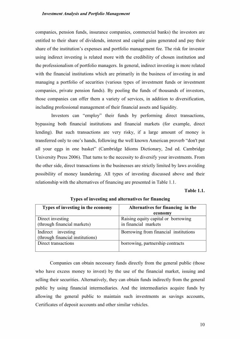
relationship with the alternatives of financing are presented in Table 1.1.
Table 1.1.
Types of investing and alternatives for financing
Types of investing in the economy Alternatives for financing in the economy
Direct investing
(through financial markets)
Raising equity capital or borrowing
in financial markets
Indirect investing
(through financial institutions)
Borrowing from financial institutions
Direct transactions
Direct borrowing, partnership contracts
Companies can obtain necessary funds directly from the general public (those
who have excess money to invest) by the use of the financial market, issuing and
selling their securities. Alternatively, they can obtain funds indirectly from the general
public by using financial intermediaries. And the intermediaries acquire funds by
allowing the general public to maintain such investments as savings accounts,
Certificates of deposit accounts and other similar vehicles.
Investment Analysis and Portfolio Management
11
1.3. Investment environment
Investment environment can be defined as the existing investment vehicles in
the market available for investor and the places for transactions with these investment
vehicles. Thus further in this subchapter the main types of investment vehicles and the
types of financial markets will be presented and described.
1.3.1. Investment vehicles
As it was presented in 1.1, in this course we are focused to the financial
investments that mean the object will be financial assets and the marketable securities
in particular. But even if further in this course only the investments in financial assets
are discussed, for deeper understanding the specifics of financial assets comparison of
some important characteristics of investment in this type of assets with the investment
in physical assets is presented.
Investment in financial assets differs from investment in physical assets in
those important aspects:
• Financial assets are divisible, whereas most physical assets are not. An
asset is divisible if investor can buy or sell small portion of it. In case of
financial assets it means, that investor, for example, can buy or sell a small
fraction of the whole company as investment object buying or selling a number
of common stocks.
• Marketability (or Liquidity) is a characteristic of financial assets that is not
shared by physical assets, which usually have low liquidity. Marketability (or
liquidity) reflects the feasibility of converting of the asset into cash quickly and
without affecting its price significantly. Most of financial assets are easy to buy
or to sell in the financial markets.
• The planned holding period of financial assets can be much shorter than the
holding period of most physical assets. The holding period for investments is
defined as the time between signing a purchasing order for asset and selling the
asset. Investors acquiring physical asset usually plan to hold it for a long
period, but investing in financial assets, such as securities, even for some
months or a year can be reasonable. Holding period for investing in financial
assets vary in very wide interval and depends on the investor’s goals and
investment strategy.
Investment Analysis and Portfolio Management
12
• Information about financial assets is often more abundant and less costly to
obtain, than information about physical assets. Information availability shows
the real possibility of the investors to receive the necessary information which
could influence their investment decisions and investment results. Since a big
portion of information important for investors in such financial assets as stocks,
bonds is publicly available, the impact of many disclosed factors having
influence on value of these securities can be included in the analysis and the
decisions made by investors.
Even if we analyze only financial investment there is a big variety of financial
investment vehicles. The on going processes of globalization and integration open
wider possibilities for the investors to invest into new investment vehicles which were
unavailable for them some time ago because of the weak domestic financial systems
and limited technologies for investment in global investment environment.
Financial innovations suggest for the investors the new choices of investment
but at the same time make the investment process and investment decisions more
complicated, because even if the investors have a wide range of alternatives to invest
they can’t forgot the key rule in investments: invest only in what you really
understand. Thus the investor must understand how investment vehicles differ from
each other and only then to pick those which best match his/her expectations.
The most important characteristics of investment vehicles on which bases the
overall variety of investment vehicles can be assorted are the return on investment and
the risk which is defined as the uncertainty about the actual return that will be earned
on an investment (determination and measurement of returns on investments and risks
will be examined in Chapter 2). Each type of investment vehicles could be
characterized by certain level of profitability and risk because of the specifics of these
financial instruments. Though all different types of investment vehicles can be
compared using characteristics of risk and return and the most risky as well as less
risky investment vehicles can be defined. However the risk and return on investment
are close related and only using both important characteristics we can really
understand the differences in investment vehicles.
The main types of financial investment vehicles are:
• Short term investment vehicles;
• Fixed-income securities;
Investment Analysis and Portfolio Management
13
• Common stock;
• Speculative investment vehicles;
• Other investment tools.
Short - term investment vehicles are all those which have a maturity of one
year or less. Short term investment vehicles often are defined as money-market
instruments, because they are traded in the money market which presents the financial
market for short term (up to one year of maturity) marketable financial assets. The risk
as well as the return on investments of short-term investment vehicles usually is lower
than for other types of investments. The main short term investment vehicles are:
• Certificates of deposit;
• Treasury bills;
• Commercial paper;
• Bankers’ acceptances;
• Repurchase agreements.
Certificate of deposit is debt instrument issued by bank that indicates a
specified sum of money has been deposited at the issuing depository institution.
Certificate of deposit bears a maturity date and specified interest rate and can be issued
in any denomination. Most certificates of deposit cannot be traded and they incur
penalties for early withdrawal. For large money-market investors financial institutions
allow their large-denomination certificates of deposits to be traded as negotiable
certificates of deposits.
Treasury bills (also called T-bills) are securities representing financial
obligations of the government. Treasury bills have maturities of less than one year.
They have the unique feature of being issued at a discount from their nominal value
and the difference between nominal value and discount price is the only sum which is
paid at the maturity for these short term securities because the interest is not paid in
cash, only accrued. The other important feature of T-bills is that they are treated as
risk-free securities ignoring inflation and default of a government, which was rare in
developed countries, the T-bill will pay the fixed stated yield with certainty. But, of
course, the yield on T-bills changes over time influenced by changes in overall
macroeconomic situation. T-bills are issued on an auction basis. The issuer accepts
competitive bids and allocates bills to those offering the highest prices. Non-
competitive bid is an offer to purchase the bills at a price that equals the average of the
Investment Analysis and Portfolio Management
14
competitive bids. Bills can be traded before the maturity, while their market price is
subject to change with changes in the rate of interest. But because of the early maturity
dates of T-bills large interest changes are needed to move T-bills prices very far. Bills
are thus regarded as high liquid assets.
Commercial paper is a name for short-term unsecured promissory notes issued
by corporation. Commercial paper is a means of short-term borrowing by large
corporations. Large, well-established corporations have found that borrowing directly
from investors through commercial paper is cheaper than relying solely on bank loans.
Commercial paper is issued either directly from the firm to the investor or through an
intermediary. Commercial paper, like T-bills is issued at a discount. The most common
maturity range of commercial paper is 30 to 60 days or less. Commercial paper is
riskier than T-bills, because there is a larger risk that a corporation will default. Also,
commercial paper is not easily bought and sold after it is issued, because the issues are
relatively small compared with T-bills and hence their market is not liquid.
Banker‘s acceptances are the vehicles created to facilitate commercial trade
transactions. These vehicles are called bankers acceptances because a bank accepts the
responsibility to repay a loan to the holder of the vehicle in case the debtor fails to
perform. Banker‘s acceptances are short-term fixed-income securities that are created
by non-financial firm whose payment is guaranteed by a bank. This short-term loan
contract typically has a higher interest rate than similar short –term securities to
compensate for the default risk. Since bankers’ acceptances are not standardized, there
is no active trading of these securities.
Repurchase agreement (often referred to as a repo) is the sale of security with
a commitment by the seller to buy the security back from the purchaser at a specified
price at a designated future date. Basically, a repo is a collectivized short-term loan,
where collateral is a security. The collateral in a repo may be a Treasury security, other
money-market security. The difference between the purchase price and the sale price is
the interest cost of the loan, from which repo rate can be calculated. Because of
concern about default risk, the length of maturity of repo is usually very short. If the
agreement is for a loan of funds for one day, it is called overnight repo; if the term of
the agreement is for more than one day, it is called a term repo. A reverse repo is the
opposite of a repo. In this transaction a corporation buys the securities with an
Investment Analysis and Portfolio Management
15
agreement to sell them at a specified price and time. Using repos helps to increase the
liquidity in the money market.
Our focus in this course further will be not investment in short-term vehicles
but it is useful for investor to know that short term investment vehicles provide the
possibility for temporary investing of money/ funds and investors use these
instruments managing their investment portfolio.
Fixed-income securities are those which return is fixed, up to some
redemption date or indefinitely. The fixed amounts may be stated in money terms or
indexed to some measure of the price level. This type of financial investments is
presented by two different groups of securities:
• Long-term debt securities
• Preferred stocks.
Long-term debt securities can be described as long-term debt instruments
representing the issuer’s contractual obligation. Long term securities have maturity
longer than 1 year. The buyer (investor) of these securities is landing money to the
issuer, who undertake obligation periodically to pay interest on this loan and repay the
principal at a stated maturity date. Long-term debt securities are traded in the capital
markets. From the investor’s point of view these securities can be treated as a “safe”
asset. But in reality the safety of investment in fixed –income securities is strongly
related with the default risk of an issuer. The major representatives of long-term debt
securities are bonds, but today there are a big variety of different kinds of bonds,
which differ not only by the different issuers (governments, municipals, companies,
agencies, etc.), but by different schemes of interest payments which is a result of
bringing financial innovations to the long-term debt securities market. As demand for
borrowing the funds from the capital markets is growing the long-term debt securities
today are prevailing in the global markets. And it is really become the challenge for
investor to pick long-term debt securities relevant to his/ her investment expectations,
including the safety of investment. We examine the different kinds of long-term debt
securities and their features important to understand for the investor in Chapter 5,
together with the other aspects in decision making investing in bonds.
Preferred stocks are equity security, which has infinitive life and pay
dividends. But preferred stock is attributed to the type of fixed-income securities,
because the dividend for preferred stock is fixed in amount and known in advance.
Investment Analysis and Portfolio Management
16
Though, this security provides for the investor the flow of income very similar to that
of the bond. The main difference between preferred stocks and bonds is that for
preferred stock the flows are for ever, if the stock is not callable. The preferred
stockholders are paid after the debt securities holders but before the common stock
holders in terms of priorities in payments of income and in case of liquidation of the
company. If the issuer fails to pay the dividend in any year, the unpaid dividends will
have to be paid if the issue is cumulative. If preferred stock is issued as noncumulative,
dividends for the years with losses do not have to be paid. Usually same rights to vote
in general meetings for preferred stockholders are suspended. Because of having the
features attributed for both equity and fixed-income securities preferred stocks is
known as hybrid security. A most preferred stock is issued as noncumulative and
callable. In recent years the preferred stocks with option of convertibility to common
stock are proliferating.
The common stock is the other type of investment vehicles which is one of
most popular among investors with long-term horizon of their investments. Common
stock represents the ownership interest of corporations or the equity of the stock
holders. Holders of common stock are entitled to attend and vote at a general meeting
of shareholders, to receive declared dividends and to receive their share of the residual
assets, if any, if the corporation is bankrupt. The issuers of the common stock are the
companies which seek to receive funds in the market and though are “going public”.
The issuing common stocks and selling them in the market enables the company to
raise additional equity capital more easily when using other alternative sources. Thus
many companies are issuing their common stocks which are traded in financial
markets and investors have wide possibilities for choosing this type of securities for
the investment. The questions important for investors for investment in common stock
decision making will be discussed in Chapter 4.
Speculative investment vehicles following the term “speculation” (see p.8)
could be defined as investments with a high risk and high investment return. Using
these investment vehicles speculators try to buy low and to sell high, their primary
concern is with anticipating and profiting from the expected market fluctuations. The
only gain from such investments is the positive difference between selling and
purchasing prices. Of course, using short-term investment strategies investors can use
for speculations other investment vehicles, such as common stock, but here we try to
Investment Analysis and Portfolio Management
17
accentuate the specific types of investments which are more risky than other
investment vehicles because of their nature related with more uncertainty about the
changes influencing the their price in the future.
Speculative investment vehicles could be presented by these different vehicles:
• Options;
• Futures;
• Commodities, traded on the exchange (coffee, grain metals, other
commodities);
Options are the derivative financial instruments. An options contract gives the
owner of the contract the right, but not the obligation, to buy or to sell a financial asset
at a specified price from or to another party. The buyer of the contract must pay a fee
(option price) for the seller. There is a big uncertainty about if the buyer of the option
will take the advantage of it and what option price would be relevant, as it depends not
only on demand and supply in the options market, but on the changes in the other
market where the financial asset included in the option contract are traded. Though, the
option is a risky financial instrument for those investors who use it for speculations
instead of hedging. The main aspects of using options for investment will be discussed
in Chapter 7.
Futures are the other type of derivatives. A future contract is an agreement
between two parties than they agree tom transact with the respect to some financial
asset at a predetermined price at a specified future date. One party agree to buy the
financial asset, the other agrees to sell the financial asset. It is very important, that in
futures contract case both parties are obligated to perform and neither party charges the
fee.
There are two types of people who deal with options (and futures) contracts:
speculators and hedgers. Speculators buy and sell futures for the sole purpose of
making a profit by closing out their positions at a price that is better than the initial
price. Such people neither produce nor use the asset in the ordinary course of business.
In contrary, hedgers buy and sell futures to offset an otherwise risky position in the
market.
Transactions using derivatives instruments are not limited to financial assets.
There are derivatives, involving different commodities (coffee, grain, precious metals,
Investment Analysis and Portfolio Management
18
and other commodities). But in this course the target is on derivatives where
underlying asset is a financial asset.
Other investment tools:
• Various types of investment funds;
• Investment life insurance;
• Pension funds;
• Hedge funds.
Investment companies/ investment funds. They receive money from investors
with the common objective of pooling the funds and then investing them in securities
according to a stated set of investment objectives. Two types of funds:
• open-end funds (mutual funds) ,
• closed-end funds (trusts).
Open-end funds have no pre-determined amount of stocks outstanding and
they can buy back or issue new shares at any point. Price of the share is not determined
by demand, but by an estimate of the current market value of the fund’s net assets per
share (NAV) and a commission.
Closed-end funds are publicly traded investment companies that have issued a
specified number of shares and can only issue additional shares through a new public
issue. Pricing of closed-end funds is different from the pricing of open-end funds: the
market price can differ from the NAV.
Insurance Companies are in the business of assuming the risks of adverse
events (such as fires, accidents, etc.) in exchange for a flow of insurance premiums.
Insurance companies are investing the accumulated funds in securities (treasury bonds,
corporate stocks and bonds), real estate. Three types of Insurance Companies: life
insurance; non-life insurance (also known as property-casualty insurance) and re-
insurance. During recent years investment life insurance became very popular
investment alternative for individual investors, because this hybrid investment product
allows to buy the life insurance policy together with possibility to invest accumulated
life insurance payments or lump sum for a long time selecting investment program
relevant to investor‘s future expectations.
Pension Funds are an asset pools that accumulates over an employee’s working
years and pays retirement benefits during the employee’s nonworking years. Pension
Investment Analysis and Portfolio Management
19
funds are investing the funds according to a stated set of investment objectives in
securities (treasury bonds, corporate stocks and bonds), real estate.
Hedge funds are unregulated private investment partnerships, limited to
institutions and high-net-worth individuals, which seek to exploit various market
opportunities and thereby to earn larger returns than are ordinarily available. They
require a substantial initial investment from investors and usually have some
restrictions on how quickly investor can withdraw their funds. Hedge funds take
concentrated speculative positions and can be very risky. It could be noted that
originally, the term “hedge” made some sense when applied to these funds. They
would by combining different types of investments, including derivatives, try to hedge
risk while seeking higher return. But today the word “hedge’ is misapplied to these
funds because they generally take an aggressive strategies investing in stock, bond and
other financial markets around the world and their level of risk is high.
1.3.2. Financial markets
Financial markets are the other important component of investment
environment.
Financial markets are designed to allow corporations and governments to raise new
funds and to allow investors to execute their buying and selling orders. In financial
markets funds are channeled from those with the surplus, who buy securities, to those,
with shortage, who issue new securities or sell existing securities. A financial market
can be seen as a set of arrangements that allows trading among its participants.
Financial market provides three important economic functions (Frank J.
Fabozzi, 1999):
1. Financial market determines the prices of assets traded through the
interactions between buyers and sellers;
2. Financial market provides a liquidity of the financial assets;
3. Financial market reduces the cost of transactions by reducing explicit costs,
such as money spent to advertise the desire to buy or to sell a financial
asset.
Financial markets could be classified on the bases of those characteristics:
• Sequence of transactions for selling and buying securities;
• Term of circulation of financial assets traded in the market;
• Economic nature of securities, traded in the market;
Investment Analysis and Portfolio Management
20
• From the perspective of a given country.
By sequence of transactions for selling and buying securities:
� Primary market
� Secondary market
All securities are first traded in the primary market, and the secondary market
provides liquidity for these securities.
Primary market is where corporate and government entities can raise capital
and where the first transactions with the new issued securities are performed. If a
company’s share is traded in the primary market for the first time this is referred to as
an initial public offering (IPO).
Investment banks play an important role in the primary market:
• Usually handle issues in the primary market;
• Among other things, act as underwriter of a new issue, guaranteeing the
proceeds to the issuer.
Secondary market - where previously issued securities are traded among
investors. Generally, individual investors do not have access to secondary markets.
They use security brokers to act as intermediaries for them. The broker delivers an
orders received form investors in securities to a market place, where these orders are
executed. Finally, clearing and settlement processes ensure that both sides to these
transactions honor their commitment. Types of brokers:
• Discount broker, who executes only trades in the secondary market;
• Full service broker, who provides a wide range of additional services to
clients (ex., advice to buy or sell);
• Online broker is a brokerage firm that allows investors to execute trades
electronically using Internet.
Types of secondary market places:
• Organized security exchanges;
• Over-the-counter markets;
• Alternative trading system.
An organized security exchange provides the facility for the members to trade
securities, and only exchange members may trade there. The members include
brokerage firms, which offer their services to individual investors, charging
commissions for executing trades on their behalf. Other exchange members by or sell
Investment Analysis and Portfolio Management
21
for their own account, functioning as dealers or market makers who set prices at which
they are willing to buy and sell for their own account. Exchanges play very important
role in the modern economies by performing the following tasks:
• Supervision of trading to ensure fairness and efficiency;
• The authorization and regulation of market participants such as brokers
and market makers;
• Creation of an environment in which securities’ prices are formed
efficiently and without distortion. This requires not only regulation of an
orders and transaction costs but also a liquid market in which there are
many buyers and sellers, allowing investors to buy or to sell their securities
quickly;
• Organization of the clearing and settlement of transactions;
• The regulation of he admission of companies to be listed on the exchange
and the regulation of companies who are listed on the exchange;
• The dissemination of information (trading data, prices and announcements
of companies listed on the exchange). Investors are more willing to trade if
prompt and complete information about trades and prices in the market is
available.
The over-the-counter (OTC) market is not a formal exchange. It is organized
network of brokers and dealers who negotiate sales of securities. There are no
membership requirements and many brokers register as dealers on the OTC. At the
same time there are no listing requirements and thousands of securities are traded in
the OTC market. OTC stocks are usually considered as very risky because they are the
stocks that are not considered large or stable enough to trade on the major exchange.
An alternative trading system (ATS) is an electronic trading mechanism
developed independently from the established market places – security exchanges –
and designed to match buyers and sellers of securities on an agency basis. The brokers
who use ATS are acting on behalf of their clients and do not trade on their own
account. The distinct advantages of ATS in comparison with traditional markets are
cost savings of transactions, the short time of execution of transactions for liquid
securities, extended hours for trading and anonymity, often important for investors,
trading large amounts.
By term of circulation of financial assets traded in the market:
Investment Analysis and Portfolio Management
22
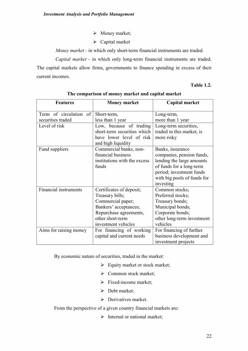
� Money market;
� Capital market
Money market - in which only short-term financial instruments are traded.
Capital market - in which only long-term financial instruments are traded.
The capital markets allow firms, governments to finance spending in excess of their
current incomes.
Table 1.2.
The comparison of money market and capital market
Features
Money market Capital market
Term of circulation of
securities traded
Short-term,
less than 1 year
Long-term,
more than 1 year
Level of risk Low, because of trading
short-term securities which
have lower level of risk
and high liquidity
Long-term securities,
traded in this market, is
more risky
Fund suppliers Commercial banks, non-
financial business
institutions with the excess
funds
Banks, insurance
companies, pension funds,
lending the large amounts
of funds for a long-term
period; investment funds
with big pools of funds for
investing
Financial instruments Certificates of deposit;
Treasury bills;
Commercial paper;
Bankers’ acceptances;
Repurchase agreements,
other short-term
investment vehicles
Common stocks;
Preferred stocks;
Treasury bonds;
Municipal bonds;
Corporate bonds;
other long-term investment
vehicles Aims for raising money For financing of working
capital and current needs
For financing of further
business development and
investment projects
By economic nature of securities, traded in the market:
� Equity market or stock market;
� Common stock market;
� Fixed-income market;
� Debt market;
� Derivatives market.
From the perspective of a given country financial markets are:
� Internal or national market;
Investment Analysis and Portfolio Management
23
� External or international market.
The internal market can be split into two fractions: domestic market and
foreign market. Domestic market is where the securities issued by domestic issuers
(companies, Government) are traded. A country’s foreign market is where the
securities issued by foreign entities are traded.
The external market also is called the international market includes the
securities which are issued at the same time to the investors in several countries and
they are issued outside the jurisdiction of any single country (for example, offshore
market).
Globalization and integration processes include the integration of financial
markets into an international financial market. Because of the globalization of financial
markets, potential issuers and investors in any country become not limited to their
domestic financial market.
1.4. Investment management process
Investment management process is the process of managing money or funds.
The investment management process describes how an investor should go about
making decisions.
Investment management process can be disclosed by five-step procedure,
which includes following stages:
1. Setting of investment policy.
2. Analysis and evaluation of investment vehicles.
3. Formation of diversified investment portfolio.
4. Portfolio revision
5. Measurement and evaluation of portfolio performance.
Setting of investment policy is the first and very important step in investment
management process. Investment policy includes setting of investment objectives. The
investment policy should have the specific objectives regarding the investment return
requirement and risk tolerance of the investor. For example, the investment policy may
define that the target of the investment average return should be 15 % and should
avoid more than 10 % losses. Identifying investor’s tolerance for risk is the most
important objective, because it is obvious that every investor would like to earn the
highest return possible. But because there is a positive relationship between risk and
return, it is not appropriate for an investor to set his/ her investment objectives as just
Investment Analysis and Portfolio Management
24
“to make a lot of money”. Investment objectives should be stated in terms of both risk
and return.
The investment policy should also state other important constrains which could
influence the investment management. Constrains can include any liquidity needs for
the investor, projected investment horizon, as well as other unique needs and
preferences of investor. The investment horizon is the period of time for investments.
Projected time horizon may be short, long or even indefinite.
Setting of investment objectives for individual investors is based on the
assessment of their current and future financial objectives. The required rate of return
for investment depends on what sum today can be invested and how much investor
needs to have at the end of the investment horizon. Wishing to earn higher income on
his / her investments investor must assess the level of risk he /she should take and to
decide if it is relevant for him or not. The investment policy can include the tax status
of the investor. This stage of investment management concludes with the identification
of the potential categories of financial assets for inclusion in the investment portfolio.
The identification of the potential categories is based on the investment objectives,
amount of investable funds, investment horizon and tax status of the investor. From the
section 1.3.1 we could see that various financial assets by nature may be more or less
risky and in general their ability to earn returns differs from one type to the other. As
an example, for the investor with low tolerance of risk common stock will be not
appropriate type of investment.
Analysis and evaluation of investment vehicles. When the investment policy
is set up, investor’s objectives defined and the potential categories of financial assets
for inclusion in the investment portfolio identified, the available investment types can
be analyzed. This step involves examining several relevant types of investment
vehicles and the individual vehicles inside these groups. For example, if the common
stock was identified as investment vehicle relevant for investor, the analysis will be
concentrated to the common stock as an investment. The one purpose of such analysis
and evaluation is to identify those investment vehicles that currently appear to be
mispriced. There are many different approaches how to make such analysis. Most
frequently two forms of analysis are used: technical analysis and fundamental analysis.
Technical analysis involves the analysis of market prices in an attempt to
predict future price movements for the particular financial asset traded on the market.
Investment Analysis and Portfolio Management
25
This analysis examines the trends of historical prices and is based on the assumption
that these trends or patterns repeat themselves in the future. Fundamental analysis in its
simplest form is focused on the evaluation of intrinsic value of the financial asset. This
valuation is based on the assumption that intrinsic value is the present value of future
flows from particular investment. By comparison of the intrinsic value and market
value of the financial assets those which are under priced or overpriced can be
identified. Fundamental analysis will be examined in Chapter 4.
This step involves identifying those specific financial assets in which to
invest and determining the proportions of these financial assets in the investment
portfolio.
Formation of diversified investment portfolio is the next step in investment
management process. Investment portfolio is the set of investment vehicles, formed by
the investor seeking to realize its’ defined investment objectives. In the stage of
portfolio formation the issues of selectivity, timing and diversification need to be
addressed by the investor. Selectivity refers to micro forecasting and focuses on
forecasting price movements of individual assets. Timing involves macro forecasting
of price movements of particular type of financial asset relative to fixed-income
securities in general. Diversification involves forming the investor’s portfolio for
decreasing or limiting risk of investment. 2 techniques of diversification:
• random diversification, when several available financial assets are put to
the portfolio at random;
• objective diversification when financial assets are selected to the portfolio
following investment objectives and using appropriate techniques for
analysis and evaluation of each financial asset.
Investment management theory is focused on issues of objective portfolio
diversification and professional investors follow settled investment objectives then
constructing and managing their portfolios.
Portfolio revision. This step of the investment management process concerns
the periodic revision of the three previous stages. This is necessary, because over time
investor with long-term investment horizon may change his / her investment objectives
and this, in turn means that currently held investor’s portfolio may no longer be
optimal and even contradict with the new settled investment objectives. Investor
should form the new portfolio by selling some assets in his portfolio and buying the
Investment Analysis and Portfolio Management
26
others that are not currently held. It could be the other reasons for revising a given
portfolio: over time the prices of the assets change, meaning that some assets that were
attractive at one time may be no longer be so. Thus investor should sell one asset ant
buy the other more attractive in this time according to his/ her evaluation. The
decisions to perform changes in revising portfolio depend, upon other things, in the
transaction costs incurred in making these changes. For institutional investors portfolio
revision is continuing and very important part of their activity. But individual investor
managing portfolio must perform portfolio revision periodically as well. Periodic re-
evaluation of the investment objectives and portfolios based on them is necessary,
because financial markets change, tax laws and security regulations change, and other
events alter stated investment goals.
Measurement and evaluation of portfolio performance. This the last step in
investment management process involves determining periodically how the portfolio
performed, in terms of not only the return earned, but also the risk of the portfolio. For
evaluation of portfolio performance appropriate measures of return and risk and
benchmarks are needed. A benchmark is the performance of predetermined set of
assets, obtained for comparison purposes. The benchmark may be a popular index of
appropriate assets – stock index, bond index. The benchmarks are widely used by
institutional investors evaluating the performance of their portfolios.
It is important to point out that investment management process is continuing
process influenced by changes in investment environment and changes in investor’s
attitudes as well. Market globalization offers investors new possibilities, but at the
same time investment management become more and more complicated with growing
uncertainty.
Summary
1. The common target of investment activities is to “employ” the money (funds)
during the time period seeking to enhance the investor’s wealth. By foregoing
consumption today and investing their savings, investors expect to enhance their
future consumption possibilities by increasing their wealth.
2. Corporate finance area of studies and practice involves the interaction between
firms and financial markets and Investments area of studies and practice involves
the interaction between investors and financial markets. Both Corporate Finance
and Investments are built upon a common set of financial principles, such as the
Investment Analysis and Portfolio Management
27
present value, the future value, the cost of capital). And very often investment and
financing analysis for decision making use the same tools, but the interpretation of
the results from this analysis for the investor and for the financier would be
different.
3. Direct investing is realized using financial markets and indirect investing involves
financial intermediaries. The primary difference between these two types of
investing is that applying direct investing investors buy and sell financial assets
and manage individual investment portfolio themselves; contrary, using indirect
type of investing investors are buying or selling financial instruments of financial
intermediaries (financial institutions) which invest large pools of funds in the
financial markets and hold portfolios. Indirect investing relieves investors from
making decisions about their portfolio.
4. Investment environment can be defined as the existing investment vehicles in the
market available for investor and the places for transactions with these investment
vehicles.
5. The most important characteristics of investment vehicles on which bases the
overall variety of investment vehicles can be assorted are the return on investment
and the risk which is defined as the uncertainty about the actual return that will be
earned on an investment. Each type of investment vehicles could be characterized
by certain level of profitability and risk because of the specifics of these financial
instruments. The main types of financial investment vehicles are: short- term
investment vehicles; fixed-income securities; common stock; speculative
investment vehicles; other investment tools.
6. Financial markets are designed to allow corporations and governments to raise new
funds and to allow investors to execute their buying and selling orders. In financial
markets funds are channeled from those with the surplus, who buy securities, to
those, with shortage, who issue new securities or sell existing securities.
7. All securities are first traded in the primary market, and the secondary market
provides liquidity for these securities. Primary market is where corporate and
government entities can raise capital and where the first transactions with the new
issued securities are performed. Secondary market - where previously issued
securities are traded among investors. Generally, individual investors do not have
Investment Analysis and Portfolio Management
28
access to secondary markets. They use security brokers to act as intermediaries for
them.
8. Financial market, in which only short-term financial instruments are traded, is
Money market, and financial market in which only long-term financial instruments
are traded is Capital market.
9. The investment management process describes how an investor should go about
making decisions. Investment management process can be disclosed by five-step
procedure, which includes following stages: (1) setting of investment policy; (2)
analysis and evaluation of investment vehicles; (3) formation of diversified
investment portfolio; (4) portfolio revision; (5) measurement and evaluation of
portfolio performance.
10. Investment policy includes setting of investment objectives regarding the
investment return requirement and risk tolerance of the investor. The other
constrains which investment policy should include and which could influence the
investment management are any liquidity needs, projected investment horizon and
preferences of the investor.
11. Investment portfolio is the set of investment vehicles, formed by the investor
seeking to realize its’ defined investment objectives. Selectivity, timing and
diversification are the most important issues in the investment portfolio formation.
Selectivity refers to micro forecasting and focuses on forecasting price movements
of individual assets. Timing involves macro forecasting of price movements of
particular type of financial asset relative to fixed-income securities in general.
Diversification involves forming the investor’s portfolio for decreasing or limiting
risk of investment.
Key-terms
• Alternative trading system
(ATS)
• Broker
• Capital market
• Closed-end funds
• Common stock
• Debt securities
• Derivatives
• Direct investing
• Diversification
• Financial institutions
• Financial intermediaries
• Financial investments
• Financial markets
• Indirect investing
• Institutional investors
Investment Analysis and Portfolio Management
29
• Investment
• Investment environment
• Investment vehicles
• Investment management
process
• Investment policy
• Investment horizon
• Investment management
• Investment funds
• Investment portfolio
• Investment life insurance
• Hedge funds
• Investment portfolio
• Long-term investments
• Money market
• Open-end funds
• Organized security exchange
• Over-the-counter (OTC)
market
• Pension funds
• Primary market
• Preferred stock
• Real investments
• Secondary market
• Short-term investments
• Speculation
• Speculative investment
Questions and problems
1. Distinguish investment and speculation.
2. Explain the difference between direct and indirect investing.
3. How could you describe the investment environment?
4. Classify the following types of financial assets as long-term and short term:
a) Repurchase agreements
b) Treasury Bond
c) Common stock
d) Commercial paper
e) Preferred Stock
f) Certificate of Deposit
5. Comment the differences between investment in financial and physical assets
using following characteristics:
a) Divisibility
b) Liquidity
c) Holding period
d) Information ability
6. Why preferred stock is called hybrid financial security?
7. Why Treasury bills considered being a risk free investment?
Investment Analysis and Portfolio Management
30
8. Describe how investment funds, pension funds and life insurance companies each
act as financial intermediaries.
9. Distinguish closed-end funds and open-end funds.
10. How do you understand why word “hedge’ currently is misapplied to hedge
funds?
11. Explain the differences between
a) Money market and capital market;
b) Primary market and secondary market.
12. Why the role of the organized stock exchanges is important in the modern
economies?
13. What factors might an individual investor take into account in determining his/
her investment policy?
14. Define the objective and the content of a five-step procedure.
15. What are the differences between technical and fundamental analysis?
16. Explain why the issues of selectivity, timing and diversification are important
when forming the investment portfolio.
17. Think about your investment possibilities for 3 years holding period in real
investment environment.
a) What could be your investment objectives?
b) What amount of funds you could invest for 3 years period?
c) What investment vehicles could you use for investment? (What types of
investment vehicles are available in your investment environment?)
d) What type(-es) of investment vehicles would be relevant to you? Why?
e) What factors would be critical for your investment decision making in
this particular investment environment?
References and further readings
1. Black, John, Nigar Hachimzade, Gareth Myles (2009). Oxford Dictionary of
Economics. 3rd
ed. Oxford University Press Inc., New York.
2. Bode, Zvi, Alex Kane, Alan J. Marcus (2005). Investments. 6th ed. McGraw
Hill.
3. Fabozzi, Frank J. (1999). Investment Management. 2nd. ed. Prentice Hall Inc.
4. Francis, Jack C., Roger Ibbotson (2002). Investments: A Global Perspective.
Prentice Hall Inc.
Investment Analysis and Portfolio Management
31
5. Haan, Jakob, Sander Oosterloo, Dirk Schoenmaker (2009).European Financial
Markets and Institutions. Cambridge University Press.
6. Jones, Charles P. (2010). Investments Principles and Concepts. John Wiley &
Sons, Inc.
7. LeBarron, Dean, Romesh Vaitlingam (1999). Ultimate Investor. Capstone.
8. Levy, Haim, Thierry Post (2005). Investments. FT / Prentice Hall.
9. Rosenberg, Jerry M. (1993).Dictionary of Investing. John Wiley &Sons Inc.
10. Sharpe, William F. Gordon J.Alexander, Jeffery V.Bailey. (1999). Investments.
International edition. Prentice –Hall International.
Relevant websites
• www.cmcmarkets.co.uk CMC Markets
• www.dcxworld.com Development Capital Exchange
• www.euronext.com Euronext
• www.nasdaqomx.com NASDAQ OMX
• www.world-exchanges.org World Federation of Exchange
• www.hedgefund.net Hedge Fund
• www.liffeinvestor.com Information and learning tools from LIFFE to
help the private investor
• www.amfi.com Association of Mutual Funds Investors
• www.standardpoors.com Standard &Poors Funds
• www.bloomberg.com/markets Bloomberg
Investment Analysis and Portfolio Management
32
2. Quantitative methods of investment analysis
Mini-contents
2.1. Investment income and risk.
2.1.1. Return on investment and expected rate of return.
2.1.2. Investment risk. Variance and standard deviation.
2.2. Relationship between risk and return.
2.2.1. Covariance.
2.2.2. Correlation and Coefficient of determination.
2.3. Relationship between the returns on asset and market portfolio
2.3.1. The characteristic line and the Beta factor.
2.3.2. Residuale variance.
Summary
Key terms
Questions and problems
References and further readings
3 basic questions for the investor in decision making:
1. How to compare different assets in investment selection process? What are
the quantitative characteristics of the assets and how to measure them?
2. How does one asset in the same portfolio influence the other one in the
same portfolio? And what could be the influence of this relationship to the investor’s
portfolio?
3. What is relationship between the returns on an asset and returns in the
whole market (market portfolio)?
The answers of these questions need quantitative methods of analysis, based on
the statistical concepts and they will be examined in this chapter.
2.1. Investment income and risk
A return is the ultimate objective for any investor. But a relationship between
return and risk is a key concept in finance. As finance and investments areas are built
upon a common set of financial principles, the main characteristics of any investment
are investment return and risk. However to compare various alternatives of
investments the precise quantitative measures for both of these characteristics are
needed.
2.1.1. Return on investment and expected rate of return
General definition of return is the benefit associated with an investment. In
most cases the investor can estimate his/ her historical return precisely.
Investment Analysis and Portfolio Management
33
Many investments have two components of their measurable return:
� a capital gain or loss;
� some form of income.
The rate of return is the percentage increase in returns associated with the
holding period:
Rate of return = Income + Capital gains / Purchase price (%) (2.1)
For example, rate of return of the share (r) will be estimated:
D + (Pme - Pmb) R = ------------------------------- (%) (2.2) Pmb Here D - dividends;
Pmb - market price of stock at the beginning of holding period;
Pme - market price of stock at the end of the holding period.
The rate of return, calculated in formulas 2.2 and 2.3 is called holding period
return, because its calculation is independent of the passages of the time. All the
investor knows is that there is a beginning of the investment period and an end. The
percent calculated using this formula might have been earned over one month or other
the year. Investor must be very careful with the interpretation of holding period returns
in investment analysis. Investor can‘t compare the alternative investments using
holding period returns, if their holding periods (investment periods) are different.
Statistical data which can be used for the investment analysis and portfolio formation
deals with a series of holding period returns. For example, investor knows monthly
returns for a year of two stocks. How he/ she can compare these series of returns? In
these cases arithmetic average return or sample mean of the returns (ř) can be
used:
n
∑∑∑∑ ri i=1
ř = ---------, (2.3) n
here ri - rate of return in period i;
n - number of observations.
Investment Analysis and Portfolio Management
34
But both holding period returns and sample mean of returns are calculated
using historical data. However what happened in the past for the investor is not as
important as what happens in the future, because all the investors‘decisions are
focused to the future, or to expected results from the investments. Of course, no one
investor knows the future, but he/ she can use past information and the historical data
as well as to use his knowledge and practical experience to make some estimates about
it. Analyzing each particular investment vehicle possibilities to earn income in the
future investor must think about several „scenarios“ of probable changes in macro
economy, industry and company which could influence asset prices ant rate of return.
Theoretically it could be a series of discrete possible rates of return in the future for the
same asset with the different probabilities of earning the particular rate of return. But
for the same asset the sum of all probabilities of these rates of returns must be equal to
1 or 100 %. In mathematical statistics it is called simple probability distribution.
The expected rate of return E(r) of investment is the statistical measure of
return, which is the sum of all possible rates of returns for the same investment
weighted by probabilities:
n
E(r) = ∑∑∑∑ hi ×××× ri , (2.4) i = 1
Here hi - probability of rate of return;
ri - rate of return.
In all cases than investor has enough information for modeling of future
scenarios of changes in rate of return for investment, the decisions should be based on
estimated expected rate of return. But sometimes sample mean of return (arithmetic
average return) are a useful proxy for the concept of expected rate of return. Sample
mean can give an unbiased estimate of the expected value, but obviously it‘s not
perfectly accurate, because based on the assumption that the returns in the future will
be the same as in the past. But this is the only one scenario in estimating expected rate
of return. It could be expected, that the accuracy of sample mean will increase, as the
size of the sample becomes longer (if n will be increased). However, the assumption,
that the underlying probability distribution does not change its shape for the longer
period becomes more and more unrealistic. In general, the sample mean of returns
should be taken for as long time, as investor is confident there has not been significant
change in the shape of historical rate of return probability distribution.
Investment Analysis and Portfolio Management
35
2.1.2. Investment risk
Risk can be defined as a chance that the actual outcome from an investment
will differ from the expected outcome. Obvious, that most investors are concerned that
the actual outcome will be less than the expected outcome. The more variable the
possible outcomes that can occur, the greater the risk. Risk is associated with the
dispersion in the likely outcome. And dispersion refers to variability. So, the total risk
of investments can be measured with such common absolute measures used in
statistics as
• variance;
• standard deviation.
Variance can be calculated as a potential deviation of each possible investment
rate of return from the expected rate of return:
n
δδδδ²(r) = ∑∑∑∑ hi ×××× [[[[ ri - E(r) ]]]]² (2.5) i=1
To compute the variance in formula 2.5 all the rates of returns which were
observed in estimating expected rate of return (ri) have to be taken together with their
probabilities of appearance (hi).
The other an equivalent to variance measure of the total risk is standard
deviation which is calculated as the square root of the variance:
______________
δδδδ(r) = √ ∑∑∑∑ hi ××××[ri - E(r)]² (2.6) In the cases than the arithmetic average return or sample mean of the returns
(ř) is used instead of expected rate of return, sample variance (δδδδ²r ) can be calculated:
n
∑∑∑∑ (rt - ř) ² t=1
δδδδ²r = -------------------- (2.7) n– 1
Sample standard deviation (δδδδr) consequently can be calculated as the square
root of the sample variance:
____
δδδδr = √ δδδδ²r (2.8)
Investment Analysis and Portfolio Management
36
Variance and the standard deviation are similar measures of risk and can be
used for the same purposes in investment analysis; however, standard deviation in
practice is used more often.
Variance and standard deviation are used when investor is focused on
estimating total risk that could be expected in the defined period in the future. Sample
variance and sample standard deviation are more often used when investor evaluates
total risk of his /her investments during historical period – this is important in
investment portfolio management.
2.2. Relationship between risk and return
The expected rate of return and the variance or standard deviation provide
investor with information about the nature of the probability distribution associated
with a single asset. However all these numbers are only the characteristics of return
and risk of the particular asset. But how does one asset having some specific trade-off
between return and risk influence the other one with the different characteristics of
return and risk in the same portfolio? And what could be the influence of this
relationship to the investor’s portfolio? The answers to these questions are of great
importance for the investor when forming his/ her diversified portfolio. The statistics
that can provide the investor with the information to answer these questions are
covariance and correlation coefficient. Covariance and correlation are related and they
generally measure the same phenomenon – the relationship between two variables.
Both concepts are best understood by looking at the math behind them.
2.2.1. Covariance
Two methods of covariance estimation can be used: the sample covariance
and the population covariance.
The sample covariance is estimated than the investor hasn‘t enough
information about the underlying probability distributions for the returns of two assets
and then the sample of historical returns is used.
Sample covariance between two assets - A and B is defined in the next
formula (2.9):
n
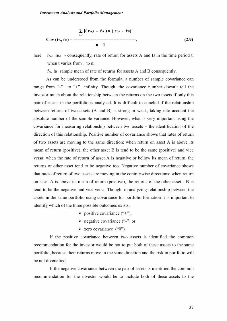
Investment Analysis and Portfolio Management
37
∑∑∑∑ [( rA,t - ŕA ) ×××× ( rB,t - ŕB)] t=1
Cov (ŕA, ŕB) = -----------------------------------------, (2.9) n – 1
here rA,t , rB,t - consequently, rate of return for assets A and B in the time period t,
when t varies from 1 to n;
ŕA, ŕB - sample mean of rate of returns for assets A and B consequently.
As can be understood from the formula, a number of sample covariance can
range from “–” to “+” infinity. Though, the covariance number doesn’t tell the
investor much about the relationship between the returns on the two assets if only this
pair of assets in the portfolio is analysed. It is difficult to conclud if the relationship
between returns of two assets (A and B) is strong or weak, taking into account the
absolute number of the sample variance. However, what is very important using the
covariance for measuring relationship between two assets – the identification of the
direction of this relationship. Positive number of covariance shows that rates of return
of two assets are moving to the same direction: when return on asset A is above its
mean of return (positive), the other asset B is tend to be the same (positive) and vice
versa: when the rate of return of asset A is negative or bellow its mean of return, the
returns of other asset tend to be negative too. Negative number of covariance shows
that rates of return of two assets are moving in the contrariwise directions: when return
on asset A is above its mean of return (positive), the returns of the other asset - B is
tend to be the negative and vice versa. Though, in analyzing relationship between the
assets in the same portfolio using covariance for portfolio formation it is important to
identify which of the three possible outcomes exists:
� positive covariance (“+”),
� negative covariance (“-”) or
� zero covariance (“0”).
If the positive covariance between two assets is identified the common
recommendation for the investor would be not to put both of these assets to the same
portfolio, because their returns move in the same direction and the risk in portfolio will
be not diversified.
If the negative covariance between the pair of assets is identified the common
recommendation for the investor would be to include both of these assets to the
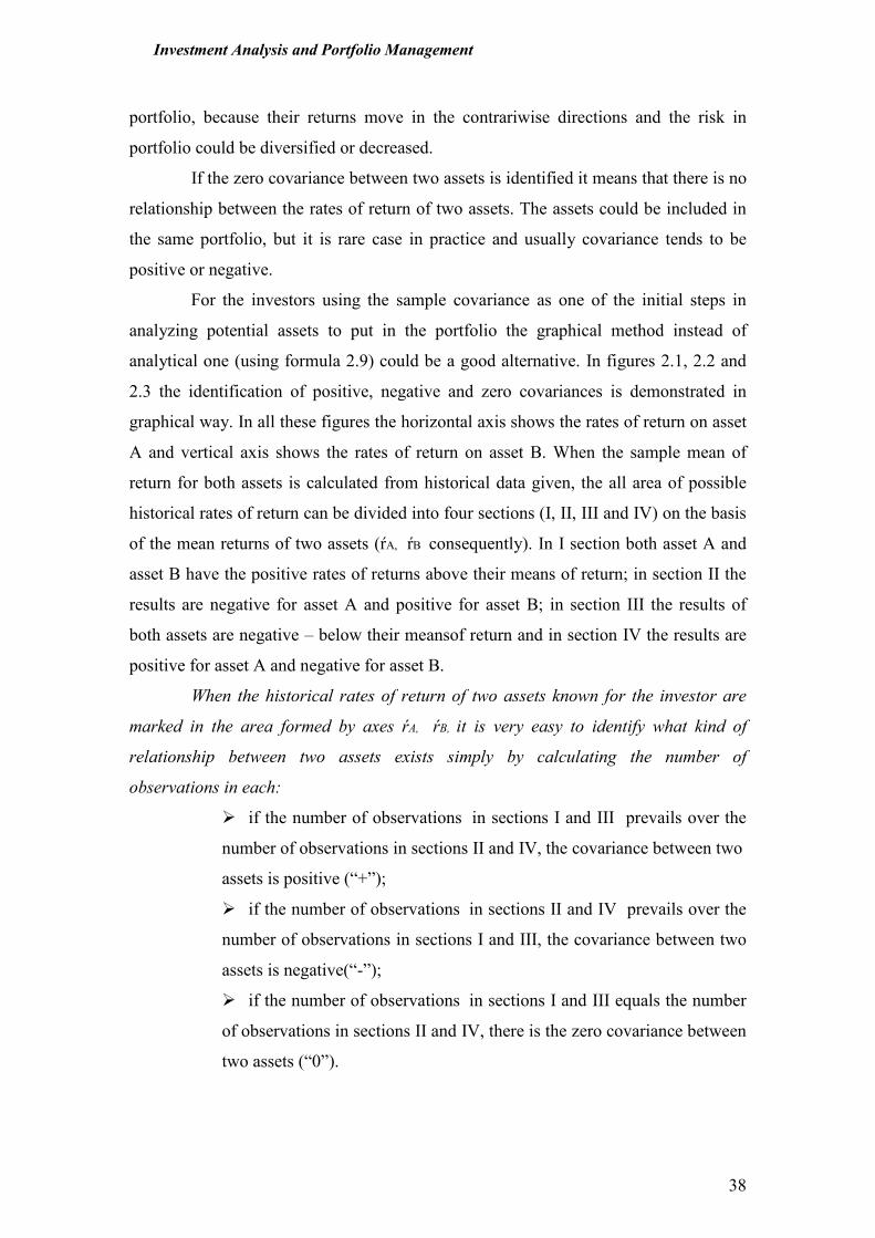
Investment Analysis and Portfolio Management
38
portfolio, because their returns move in the contrariwise directions and the risk in
portfolio could be diversified or decreased.
If the zero covariance between two assets is identified it means that there is no
relationship between the rates of return of two assets. The assets could be included in
the same portfolio, but it is rare case in practice and usually covariance tends to be
positive or negative.
For the investors using the sample covariance as one of the initial steps in
analyzing potential assets to put in the portfolio the graphical method instead of
analytical one (using formula 2.9) could be a good alternative. In figures 2.1, 2.2 and
2.3 the identification of positive, negative and zero covariances is demonstrated in
graphical way. In all these figures the horizontal axis shows the rates of return on asset
A and vertical axis shows the rates of return on asset B. When the sample mean of
return for both assets is calculated from historical data given, the all area of possible
historical rates of return can be divided into four sections (I, II, III and IV) on the basis
of the mean returns of two assets (ŕA, ŕB consequently). In I section both asset A and
asset B have the positive rates of returns above their means of return; in section II the
results are negative for asset A and positive for asset B; in section III the results of
both assets are negative – below their meansof return and in section IV the results are
positive for asset A and negative for asset B.
When the historical rates of return of two assets known for the investor are
marked in the area formed by axes ŕA, ŕB, it is very easy to identify what kind of
relationship between two assets exists simply by calculating the number of
observations in each:
� if the number of observations in sections I and III prevails over the
number of observations in sections II and IV, the covariance between two
assets is positive (“+”);
� if the number of observations in sections II and IV prevails over the
number of observations in sections I and III, the covariance between two
assets is negative(“-”);
� if the number of observations in sections I and III equals the number
of observations in sections II and IV, there is the zero covariance between
two assets (“0”).
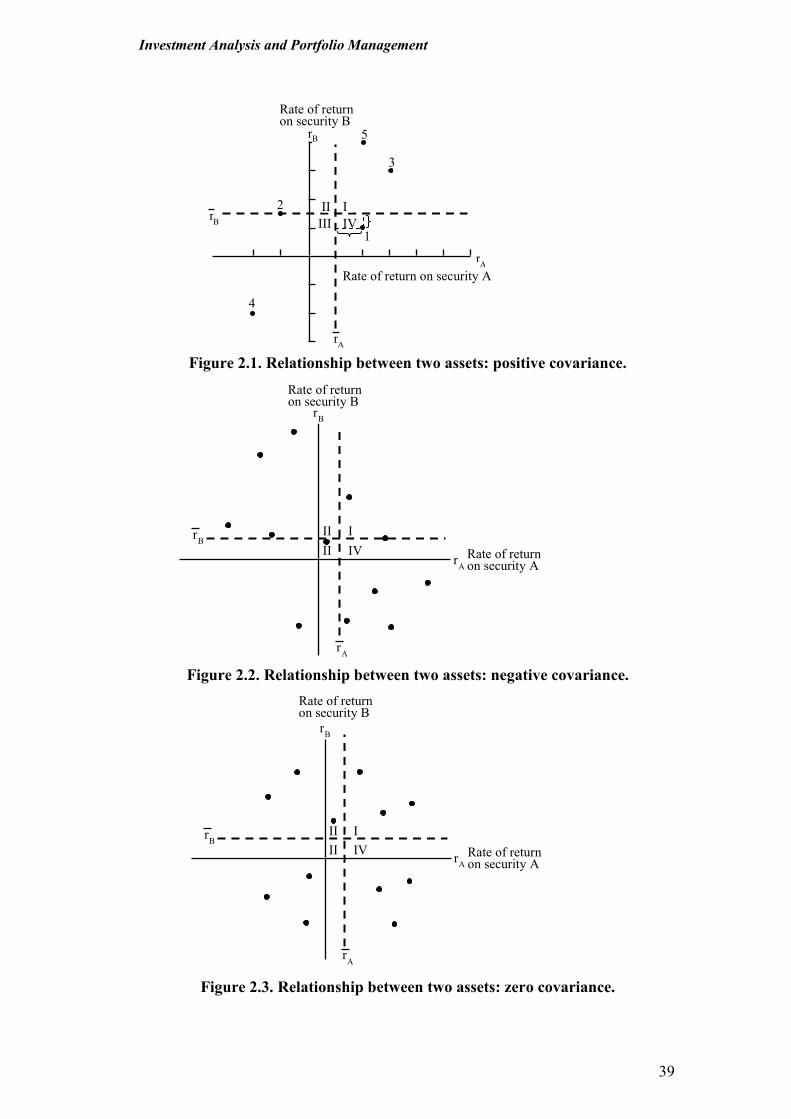
Investment Analysis and Portfolio Management
39
Figure 2.1. Relationship between two assets: positive covariance.
Figure 2.2. Relationship between two assets: negative covariance.
Figure 2.3. Relationship between two assets: zero covariance.
Rate of return on security B
2
1
IV
r
A
II I
III
Rate of return on security A
r
A
r
B
4
5
3
r B
IV
r
B
Rate of return on security B
r
A
II I
II Rate of return on security A
r
A
r
B
IV
r
B
Rate of return on security B
r
A
II I
II Rate of return on security A
r
A
r
B
Investment Analysis and Portfolio Management
40
The population covariance is estimated when the investor has enough
information about the underlying probability distributions for the returns of two assets
and can identify the actual probabilities of various pairs of the returns for two assets at
the same time.
The population covariance between stocks A and B:
m
Cov (rA, rB) = ∑∑∑∑ hi ×××× [[[[rA,i - E(rA) ]]]] ×××× [[[[rB,i - E(rB)]]]] (2.10) i=1
Similar to using the sample covariance, in the population covariance case the
graphical method can be used for the identification of the direction of the relationship
between two assets. But the graphical presentation of data in this case is more
complicated because three dimensions must be used (including the probability).
Despite of it, if investor observes that more pairs of returns are in the sections I and III
than in II and IV, the population covariance will be positive, if the pairs of return in II
and IV prevails over I and III, the population covariance is negative.
2.2.2. Correlation and Coefficient of determination.
Correlation is the degree of relationship between two variables.
The correlation coefficient between two assets is closely related to their
covariance. The correlation coefficient between two assets A and B (kAB) can be
calculated using the next formula:
Cov(rA,rB) kA,B = ------------------- , (2.11) δδδδ (rA) ×××× δδδδ(rB)
here δ (rA) and δ(rB) are standard deviation for asset A and B consequently.
Very important, that instead of covariance when the calculated number is
unbounded, the correlation coefficient can range only from -1,0 to +1,0. The more
close the absolute meaning of the correlation coefficient to 1,0, the stronger the
relationship between the returns of two assets. Two variables are perfectly positively
correlated if correlation coefficient is +1,0, that means that the returns of two assets
have a perfect positive linear relationship to each other (see Fig. 2.4), and perfectly
negatively correlated if correlation coefficient is -1,0, that means the asset returns
have a perfect inverse linear relationship to each other (see Fig. 2.5). But most often
correlation between assets returns is imperfect (see Fig. 2.6). When correlation
coefficient equals 0, there is no linear relationship between the returns on the two

Investment Analysis and Portfolio Management
41
assets (see Fig. 2.7). Combining two assets with zero correlation with each other
reduces the risk of the portfolio. While a zero correlation between two assets returns
is better than positive correlation, it does not provide the risk reduction results of a
negative correlation coefficient.
Fig. 2.4. Perfect positive correlation Fig. 2.5. Perfect negative correlation between returns of two assets. between returns of two assets. .
Fig. 2.6. Imperfect positive correlation Fig. 2.7. Zero correlation between between returns on two assets. returns on two assets.
r
B
r
A
r
B
r
A
r
B
r
A
r
B
r
A
Investment Analysis and Portfolio Management
42
It can be useful to note, that when investor knows correlation coefficient, the
covariance between stocks A and B can be estimated, because standard deviations of
the assets’ rates of return will already are available:
Cov(rA, rB ) = kA,B ×××× δδδδ(rA) ×××× δδδδ (rB) (2.12)
Therefore, as it was pointed out earlier, the covariance primarily provides
information to the investor about whether the relationship between asset returns is
positive, negative or zero, because simply observing the number itself without any
context with which to compare the number, is not very useful. When the covariance is
positive, the correlation coefficient will be also positive, when the covariance is
negative, the correlation coefficient will be also negative. But using correlation
coefficients instead of covariance investor can immediately asses the degree of
relationship between assets returns.
The coefficient of determination (Det.AB) is calculated as the square of
correlation coefficient:
Det.A, B = k²A,B (2.13) The coefficient of determination shows how much variability in the returns of
one asset can be associated with variability in the returns of the other. For example, if
correlation coefficient between returns of two assets is estimated + 0,80, the coefficient
of determination will be 0,64. The interpretation of this number for the investor is that
approximately 64 percent of the variability in the returns of one asset can be explained
by the returns of the other asset. If the returns on two assets are perfect correlated, the
coefficient of determination will be equal to 100 %, and this means that in such a case
if investor knows what will be the changes in returns of one asset he / she could predict
exactly the return of the other asset.
2.3. Relationship between the returns on stock and market portfolio
When picking the relevant assets to the investment portfolio on the basis of
their risk and return characteristics and the assessment of the relationship of their
returns investor must consider to the fact that these assets are traded in the market.
How could the changes in the market influence the returns of the assets in the
investor’s portfolio? What is the relationship between the returns on an asset and
returns in the whole market (market portfolio)? These questions need to be answered
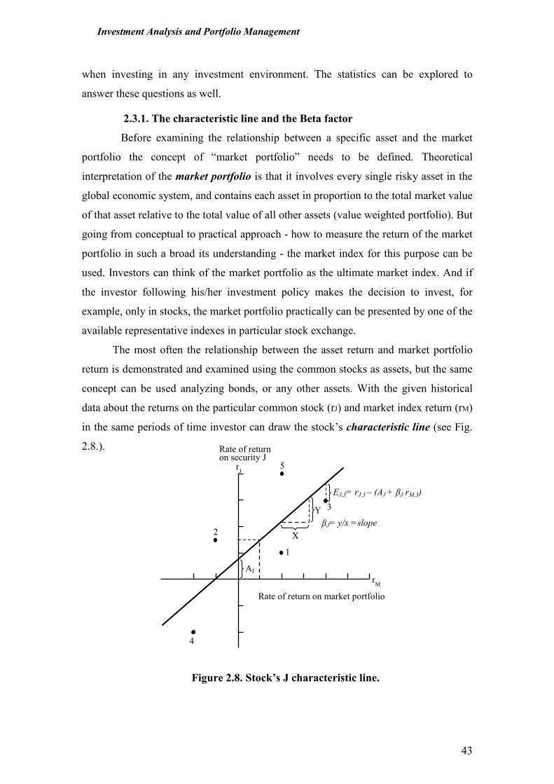
Investment Analysis and Portfolio Management
43
when investing in any investment environment. The statistics can be explored to
answer these questions as well.
2.3.1. The characteristic line and the Beta factor
Before examining the relationship between a specific asset and the market
portfolio the concept of “market portfolio” needs to be defined. Theoretical
interpretation of the market portfolio is that it involves every single risky asset in the
global economic system, and contains each asset in proportion to the total market value
of that asset relative to the total value of all other assets (value weighted portfolio). But
going from conceptual to practical approach - how to measure the return of the market
portfolio in such a broad its understanding - the market index for this purpose can be
used. Investors can think of the market portfolio as the ultimate market index. And if
the investor following his/her investment policy makes the decision to invest, for
example, only in stocks, the market portfolio practically can be presented by one of the
available representative indexes in particular stock exchange.
The most often the relationship between the asset return and market portfolio
return is demonstrated and examined using the common stocks as assets, but the same
concept can be used analyzing bonds, or any other assets. With the given historical
data about the returns on the particular common stock (rJ) and market index return (rM)
in the same periods of time investor can draw the stock’s characteristic line (see Fig.
2.8.).
Figure 2.8. Stock’s J characteristic line.
2
1
Rate of return on security J
Rate of return on market portfolio
r
M
4
5
3 Y
X
AJ
ΕJ,3= rJ,3 – (AJ + βJ rM,3)
r
J
βJ= y/x =slope
Investment Analysis and Portfolio Management
44
Stock’s characteristic line:
� describes the relationship between the stock and the market;
� shows the return investor expect the stock to produce, given that a
particular rate of return appears for the market;
� helps to assess the risk characteristics of one stock relative to the market.
Stock’s characteristic line as a straight line can be described by its slope and
by point in which it crosses the vertical axis - intercept (point A in Fig. 2.8.).
The slope of the characteristic line is called the Beta factor. Beta factor for
the stock J and can be calculated using following formula:
Cov (rJ,rM) ββββJ = ------------------- , (2.14)
δδδδ²(rM)
here: Cov(rJ,rM) – covariance between returns of stock J and the market portfolio;
δ²(rM) - variance of returns on market portfolio.
The Beta factor of the stock is an indicator of the degree to which the stock
reacts to the changes in the returns of the market portfolio. The Beta gives the answer
to the investor how much the stock return will change when the market return will
change by 1 percent. Further in Chapter 3 the use of Beta factor in developing capital
asset pricing model will be discussed.
Intercept AJ (the point where characteristic line passes through the vertical
axis) can be calculated using following formula:
AJ = rJ - ββββJ ×××× rM, (2.15)
here: rJ - rate of return of stock J;
βJ - Beta factor for the stock J;
rM - rate of return of the market.
The intercept technically is a convenient point for drawing a characteristic line.
The interpretation of the intercept from the investor’s point of view is that it shows
what would be the rate of return of the stock, if the rate of return in the market is zero.
2.3.2. Residual variance
The characteristic line is a line-of-best-fit through some data points. A
characteristic line is what in statistics is called as time-series regression line. But in
Investment Analysis and Portfolio Management
45
reality the stock produce returns that deviate from the characteristic line (see Fig. 2.8).
In statistics this propensity is called the residual variance.
Residual variance is the variance in the stock’s residuals and for the stock J
can be calculated using formula:
n
Σ εεεε²J,t t =1
δδδδ²εεεε,t = -------------- , (2.15) n - 2
here εJ,t - residual of the stock J in period t;
n - number of periods observed.
To calculate residual variance the residual in every period of observations
must be identified. Residual is the vertical distance between the point which reflect
the pair of returns (stock J and market) and the characteristic line of stock J. The
residual of the stock J can be calculated:
εεεεJ,t = rJ,t - ( AJ + ββββJ ×××× r M,t ) (2.16) c.1 c.2
It is useful for the interpretation of residual to investor to accentuate two
components in formula of residual (see 2.16):
• Component 1 reflects the return actually generated by the stock J during
period t;
• Component 2 (in the bracket) represents investor’s expectations for the
stock’s return, given its characteristic line and market’s returns.
Note the difference between the variance and the residual variance:
� The variance describes the deviation of the asset returns from its expected
value ;
� The residual variance describes the deviation of the asset returns from its
characteristic line.
Summary
1. The main characteristics of any investment are investment return and risk.
However to compare various alternatives of investments the precise quantitative
measures for both of these characteristics are needed.
2. General definition of return is the benefit associated with an investment. Many
investments have two components of their measurable return: (1) a capital gain or
Investment Analysis and Portfolio Management
46
loss; (2) some form of income. The holding period return is the percentage increase
in returns associated with the holding period.
3. Investor can‘t compare the alternative investments using holding period returns, if
their holding periods (investment periods) are different. In these cases arithmetic
average return or sample mean of the returns can be used.
4. Both holding period returns and sample mean of returns are calculated using
historical data. However all the investors’ decisions are focused to the future, or to
expected results from the investments. The expected rate of return of investment is
the statistical measure of return, which is the sum of all possible rates of returns for
the same investment weighted by probabilities.
5. Risk can be defined as a chance that the actual outcome from an investment will
differ from the expected outcome. The total risk of investments can be measured
with such common absolute measures used in statistics as variance and standard
deviation. Variance can be calculated as a potential deviation of each possible
investment rate of return from the expected rate of return. Standard deviation is
calculated as the square root of the variance. The more variable the possible
outcomes that can occur, the greater the risk.
6. In the cases than the arithmetic average return or sample mean of the returns is
used instead of expected rate of return, sample variance and sample standard
deviation is calculated.
7. Covariance and correlation coefficient are used to answer the question, what is the
relationship between the returns on different assets. Covariance and correlation
coefficient are related and they generally measure the same phenomenon – the
relationship between two variables.
8. The sample covariance is estimated than the investor hasn‘t enough information
about the underlying probability distributions for the returns of two assets and then
the sample of historical returns is used. The population covariance is estimated
when the investor has enough information about the underlying probability
distributions for the returns of two assets and can identify the actual probabilities
of various pairs of the returns for two assets at the same time.
9. Analyzing relationship between the assets in the same portfolio using covariance
for portfolio formation it is important to identify which of the three possible
outcomes exists: positive covariance, negative covariance or zero covariance. If the
Investment Analysis and Portfolio Management
47
positive covariance between two assets is identified the common recommendation
for the investor would be not to put both of these assets to the same portfolio,
because their returns move in the same direction and the risk in portfolio will be
not diversified; if the negative - the common recommendation for the investor
would be to include both of these assets to the portfolio, because their returns move
in the contrariwise directions and the risk in portfolio could be diversified; if the
zero covariance - it means that there is no relationship between the rates of return
of two assets.
10. The correlation coefficient between two assets is closely related to their
covariance. But instead of covariance when the calculated number is unbounded,
the correlation coefficient can range only from -1,0 to +1,0. The more close the
absolute meaning of the correlation coefficient to 1,0, the stronger the relationship
between the returns of two assets. Using correlation coefficients instead of
covariance investor can immediately asses the degree of relationship between
assets returns.
11. The coefficient of determination is calculated as the square of correlation
coefficient and shows how much variability in the returns of one asset can be
associated with variability in the returns of the other.
12. Theoretical interpretation of the market portfolio is that it involves every single
risky asset in the global economic system, and contains each asset in proportion to
the total market value of that asset relative to the total value of all other assets
(value weighted portfolio). Investors can think of the market portfolio as the
ultimate market index.
13. Stock’s characteristic line describes the relationship between the stock and the
market, shows the return investor expect the stock to produce, given that a
particular rate of return appears for the market and helps to assess the risk
characteristics of one stock relative to the market.
14. The slope of the characteristic line is called the Beta factor. The Beta factor of the
stock is an indicator of the degree to which the stock reacts to the changes in the
returns of the market portfolio.
15. The intercept is the point where characteristic line passes through the vertical axis.
The interpretation of the intercept from the investor’s point of view is that it shows
Investment Analysis and Portfolio Management
48
what would be the rate of return of the stock, if the rate of return in the market is
zero.
16. The residual variance describes the deviation of the asset returns from its
characteristic line.
Key-terms
• Beta factor
• Characteristic line
• Coefficient of correlation
• Coefficient of determination
• Correlation
• Covariance
• Expected rate of return
• Holding period return
• Intercept
• Investment risk
• Market portfolio
• Population covariance
• Probability
• Residual
• Residual variance
• Return on investment
• Sample mean of return
• Sample standard deviation
• Sample covariance
• Sample variance
• Simple probability distribution
• Standard deviation
• Variance
Questions and problems
1. Comment why methods and tools of the statistics are so important in investment
decision making.
2. Distinguish between historical returns and expected returns.
3. Define the components of holding period return. Can any of these components be
negative?
4. When should the sample mean of return be used instead of expected rate of return?
5. What does a probability distribution describe?
6. What does covariance measure? If two assets are said to have positive covariance,
what does it mean?
7. Explain, why doesn’t an estimated absolute covariance number tell the investor
much about the relationship between the returns on the two assets?
8. How do you understand an investment risk and what statistic tools can be used to
measure it?
Investment Analysis and Portfolio Management
49
9. What is the interpretation of the coefficient of determination for the investor? If the
coefficient of correlation for two securities is 0,7, what is the coefficient of
determination?
10. Describe the Beta factor.
11. What does the characteristic line tells to investor? Why stock characteristic lines
are different for the securities traded in the same market?
12. With which of stock’s characteristic line definitions presented below you disagree?
a) Stock’s characteristic line describes the relationship between the stock
and the market;
b) Stock’s characteristic line shows the return investor expect the stock to
produce, given that a particular rate of return appears for the market;
c) Stock’s characteristic line describes the relationship between rate of
return of any two different stocks in the market;
d) I agree with all definitions presented above.
13. Refer to the following information on joint stock returns for stock 1, 2, and 3 in
the table
Probability Return for stock Stock 1 Stock 2 Stock 3
0.20 0.20 0.25 0.10
0.30 -0.05 0.10 0.05
0.25 0.10 0.05 0
0.25 0 -0.10 -0.05
If you must choose only two stocks to your investment portfolio, what would be
your choise?
a) stocks 1 and 2; b) stocks 1 and 3; c) stocks 2 and 3; d) other decision.
Present your arguments and calculations, to explain your decision.
14. Refer to the following observations for stock A and the market portfolio in the
table:
Rate of return Month Stock A Market portfolio
1 0,30 0,12
2 0.24 0,08
3 -0,04 -0,10
4 0,10 -0,02
5 0,06 0,08
6 0,10 0,07
Investment Analysis and Portfolio Management
50
a) Calculate the main statistic measures to explain the relationship between stock
A and the market portfolio:
• The sample covariance between rate of return for the stock A and the
market;
• The sample Beta factor of stock A;
• The sample correlation coefficient between the rates of return of the
stock A and the market;
• The sample coefficient of determination associated with the stock A and
the market.
b) Draw in the characteristic line of the stock A and give the interpretation - what
does it show for the investor?
c) Calculate the sample residual variance associated with stock‘s A characteristic
line and explain how the investor would interpret the number of this statistic.
d) Do you recommend this stock for the investor with the lower tolerance of risk?
References and further readings
1. Fabozzi, Frank J. (1999). Investment Management. 2nd. ed. Prentice Hall Inc.
2. Francis, Jack, C. Roger Ibbotson (2002). Investments: A Global Perspective.
Prentice Hall Inc.
3. Haugen, (Robert A. 2001). Modern Investment Theory. 5th
ed. Prentice Hall.
4. Levy, Haim, Thierry Post (2005). Investments. FT / Prentice Hall.
5. Rosenberg, Jerry M. (1993).Dictionary of Investing. John Wiley &Sons Inc.
6. Sharpe, William F., Gordon J.Alexander, Jeffery V.Bailey. (1999). Investments.
International edition. Prentice –Hall International.
7. Strong, Robert A. (1993). Portfolio Construction, Management and Protection.
Investment Analysis and Portfolio Management
51
3. Theory for investment portfolio formation
Mini-contents
3.1. Portfolio theory.
3.1.1. Markowitz portfolio theory.
3.1.2. The Risk and Expected Return of a Portfolio.
3.2. Capital Asset Pricing Model (CAPM).
3.3. Arbitrage Pricing Theory (APT).
3.4. Market efficiency theory.
Summary
Key terms
Questions and problems
References and further readings
3.1. Portfolio theory 3.1.1. Markowitz portfolio theory
The author of the modern portfolio theory is Harry Markowitz who introduced
the analysis of the portfolios of investments in his article “Portfolio Selection”
published in the Journal of Finance in 1952. The new approach presented in this article
included portfolio formation by considering the expected rate of return and risk of
individual stocks and, crucially, their interrelationship as measured by correlation.
Prior to this investors would examine investments individually, build up portfolios of
attractive stocks, and not consider how they related to each other. Markowitz showed
how it might be possible to better of these simplistic portfolios by taking into account
the correlation between the returns on these stocks.
The diversification plays a very important role in the modern portfolio theory.
Markowitz approach is viewed as a single period approach: at the beginning of the
period the investor must make a decision in what particular securities to invest and
hold these securities until the end of the period. Because a portfolio is a collection of
securities, this decision is equivalent to selecting an optimal portfolio from a set of
possible portfolios. Essentiality of the Markowitz portfolio theory is the problem of
optimal portfolio selection.
The method that should be used in selecting the most desirable portfolio involves
the use of indifference curves. Indifference curves represent an investor’s preferences
for risk and return. These curves should be drawn, putting the investment return on the
vertical axis and the risk on the horizontal axis. Following Markowitz approach, the
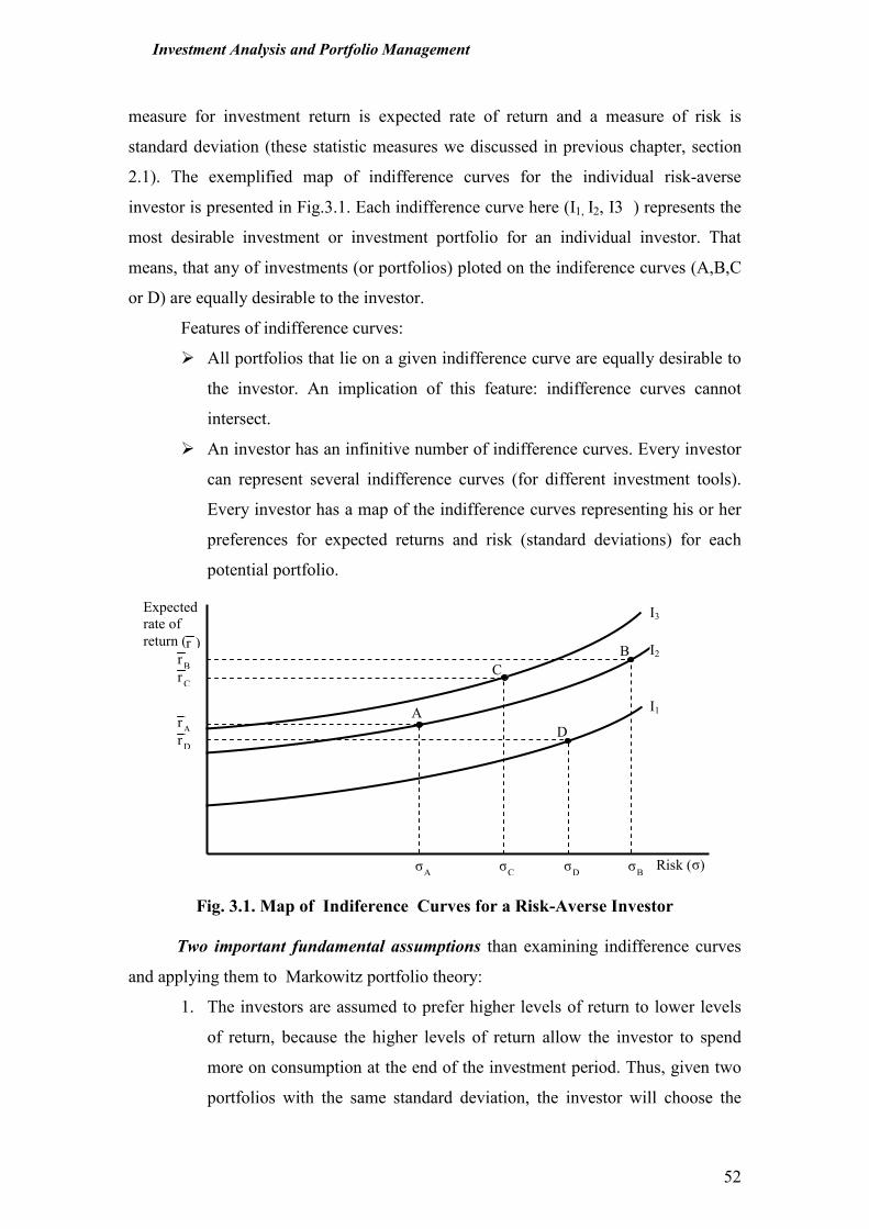
Investment Analysis and Portfolio Management
52
measure for investment return is expected rate of return and a measure of risk is
standard deviation (these statistic measures we discussed in previous chapter, section
2.1). The exemplified map of indifference curves for the individual risk-averse
investor is presented in Fig.3.1. Each indifference curve here (I1, I2, I3 ) represents the
most desirable investment or investment portfolio for an individual investor. That
means, that any of investments (or portfolios) ploted on the indiference curves (A,B,C
or D) are equally desirable to the investor.
Features of indifference curves:
� All portfolios that lie on a given indifference curve are equally desirable to
the investor. An implication of this feature: indifference curves cannot
intersect.
� An investor has an infinitive number of indifference curves. Every investor
can represent several indifference curves (for different investment tools).
Every investor has a map of the indifference curves representing his or her
preferences for expected returns and risk (standard deviations) for each
potential portfolio.
Fig. 3.1. Map of Indiference Curves for a Risk-Averse Investor
Two important fundamental assumptions than examining indifference curves
and applying them to Markowitz portfolio theory:
1. The investors are assumed to prefer higher levels of return to lower levels
of return, because the higher levels of return allow the investor to spend
more on consumption at the end of the investment period. Thus, given two
portfolios with the same standard deviation, the investor will choose the
Risk (
D
B
C
r
B
r
C
r
A
r
D
I1
I2
I3
σ B
σ D
σ C
σ A
σ
A
Expected
rate of
return (
)
r )
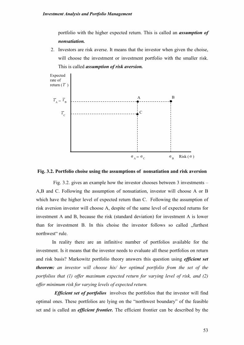
Investment Analysis and Portfolio Management
53
portfolio with the higher expected return. This is called an assumption of
nonsatiation.
2. Investors are risk averse. It means that the investor when given the choise,
will choose the investment or investment portfolio with the smaller risk.
This is called assumption of risk aversion.
Fig. 3.2. Portfolio choise using the assumptions of nonsatiation and risk aversion
Fig. 3.2. gives an example how the investor chooses between 3 investments –
A,B and C. Following the assumption of nonsatiation, investor will choose A or B
which have the higher level of expected return than C. Following the assumption of
risk aversion investor will choose A, despite of the same level of expected returns for
investment A and B, because the risk (standard deviation) for investment A is lower
than for investment B. In this choise the investor follows so called „furthest
northwest“ rule.
In reality there are an infinitive number of portfolios available for the
investment. Is it means that the investor needs to evaluate all these portfolios on return
and risk basis? Markowitz portfolio theory answers this question using efficient set
theorem: an investor will choose his/ her optimal portfolio from the set of the
portfolios that (1) offer maximum expected return for varying level of risk, and (2)
offer minimum risk for varying levels of expected return.
Efficient set of portfolios involves the portfolios that the investor will find
optimal ones. These portfolios are lying on the “northwest boundary” of the feasible
set and is called an efficient frontier. The efficient frontier can be described by the
C
B A
=
= r
A r
B
r
C
σ A
σ C
σ B
Expected
rate of
return (
Risk ( σ )
r
)
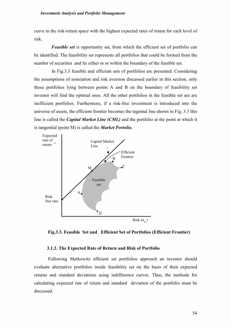
Investment Analysis and Portfolio Management
54
curve in the risk-return space with the highest expected rates of return for each level of
risk.
Feasible set is opportunity set, from which the efficient set of portfolio can
be identified. The feasibility set represents all portfolios that could be formed from the
number of securities and lie either or or within the boundary of the feasible set.
In Fig.3.3 feasible and efficient sets of portfolios are presented. Considering
the assumptions of nonsiation and risk aversion discussed earlier in this section, only
those portfolios lying between points A and B on the boundary of feasibility set
investor will find the optimal ones. All the other portfolios in the feasible set are are
inefficient portfolios. Furthermore, if a risk-free investment is introduced into the
universe of assets, the efficient frontier becomes the tagental line shown in Fig. 3.3 this
line is called the Capital Market Line (CML) and the portfolio at the point at which it
is tangential (point M) is called the Market Portolio.
Fig.3.3. Feasible Set and Efficient Set of Portfolios (Efficient Frontier)
3.1.2. The Expected Rate of Return and Risk of Portfolio
Following Markowitz efficient set portfolios approach an investor should
evaluate alternative portfolios inside feasibility set on the basis of their expected
returns and standard deviations using indifference curves. Thus, the methods for
calculating expected rate of return and standard deviation of the portfolio must be
discussed.
A
M
C
A
Feasible
set
B
C
D
Risk (
Expected
rate of
return
σ P
)
Risk
free rate
Capital Market
Line
Efficient
Frontier
Investment Analysis and Portfolio Management
55
The expected rate of return of the portfolio can be calculated in some
alternative ways. The Markowitz focus was on the end-of-period wealth (terminal
value) and using these expected end-of-period values for each security in the portfolio
the expected end-of-period return for the whole portfolio can be calculated. But the
portfolio really is the set of the securities thus the expected rate of return of a portfolio
should depend on the expected rates of return of each security included in the portfolio
(as was presented in Chapter 2, formula 2.4). This alternative method for calculating
the expected rate of return on the portfolio (E(r)p) is the weighted average of the
expected returns on its component securities:
n
E(r)p = Σ wi * Ei (r) = E1(r) + w2 * E2(r) +…+ wn * En(r), (3.1) i=1
here wi - the proportion of the portfolio’s initial value invested in security i;
Ei(r) - the expected rate of return of security I;
n - the number of securities in the portfolio.
Because a portfolio‘s expected return is a weighted average of the expected
returns of its securities, the contribution of each security to the portfolio‘s expected
rate of return depends on its expected return and its proportional share from the initial
portfolio‘s market value (weight). Nothing else is relevant. The conclusion here could
be that the investor who simply wants the highest posible expected rate of return must
keep only one security in his portfolio which has a highest expected rate of return. But
why the majority of investors don‘t do so and keep several different securities in their
portfolios? Because they try to diversify their portfolios aiming to reduce the
investment portfolio risk.
Risk of the portfolio. As we know from chapter 2, the most often used
measure for the risk of investment is standard deviation, which shows the volatility of
the securities actual return from their expected return. If a portfolio‘s expected rate of
return is a weighted average of the expected rates of return of its securities, the
calculation of standard deviation for the portfolio can‘t simply use the same approach.
The reason is that the relationship between the securities in the same portfolio must be
taken into account. As it was discussed in section 2.2, the relationship between the
assets can be estimated using the covariance and coefficient of correlation. As
covariance can range from “–” to “+” infinity, it is more useful for identification of
the direction of relationship (positive or negative), coefficients of correlation always
Investment Analysis and Portfolio Management
56
lies between -1 and +1 and is the convenient measure of intensity and direction of the
relationship between the assets.
Risk of the portfolio, which consists of 2 securities (A ir B):
δδδδp = (w²A ×××× δδδδ²A + w²B ××××δδδδ²B + 2 wA ×××× wB ×××× kAB ×××× δδδδA××××δδδδB)1/2, (3.2)
here: wA ir wB - the proportion of the portfolio’s initial value invested in security A
and B ( wA + wB = 1);
δA ir δB - standard deviation of security A and B;
kAB - coefficient of coreliation between the returns of security A and B.
Standard deviation of the portfolio consisting n securities: n n
δδδδ = ( ∑∑∑∑ ∑∑∑∑ wi wj kij δδδδi δδδδj )1/2 , (3.3) i=1 j=1
here: wi ir wj - the proportion of the portfolio’s initial value invested in security i
and j ( wi + wj = 1);
δi ir δj - standard deviation of security i and j;
kij - coefficient of coreliation between the returns of security i and j.
3.2. Capital Asset Pricing Model (CAPM)
CAPM was developed by W. F. Sharpe. CAPM simplified Markowitz‘s Modern
Portfolio theory, made it more practical. Markowitz showed that for a given level of
expected return and for a given feasible set of securities, finding the optimal portfolio
with the lowest total risk, measured as variance or standard deviation of portfolio
returns, requires knowledge of the covariance or correlation between all possible
security combinations (see formula 3.3). When forming the diversified portfolios
consisting large number of securities investors found the calculation of the portfolio
risk using standard deviation technically complicated.
Measuring Risk in CAPM is based on the identification of two key
components of total risk (as measured by variance or standard deviation of return):
� Systematic risk
� Unsystematic risk
Systematic risk is that associated with the market (purchasing power risk,
interest rate risk, liquidity risk, etc.)
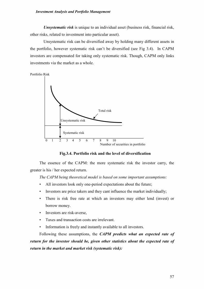
Investment Analysis and Portfolio Management
57
Unsystematic risk is unique to an individual asset (business risk, financial risk,
other risks, related to investment into particular asset).
Unsystematic risk can be diversified away by holding many different assets in
the portfolio, however systematic risk can’t be diversified (see Fig 3.4). In CAPM
investors are compensated for taking only systematic risk. Though, CAPM only links
investments via the market as a whole.
Portfolio Risk
0 1 2 3 4 5 6 7 8 9 10
Number of securities in portfolio
Fig.3.4. Portfolio risk and the level of diversification
The essence of the CAPM: the more systematic risk the investor carry, the
greater is his / her expected return.
The CAPM being theoretical model is based on some important assumptions:
• All investors look only one-period expectations about the future;
• Investors are price takers and they cant influence the market individually;
• There is risk free rate at which an investors may either lend (invest) or
borrow money.
• Investors are risk-averse,
• Taxes and transaction costs are irrelevant.
• Information is freely and instantly available to all investors.
Following these assumptions, the CAPM predicts what an expected rate of
return for the investor should be, given other statistics about the expected rate of
return in the market and market risk (systematic risk):
Systematic risk
Unsystematic risk
Total risk
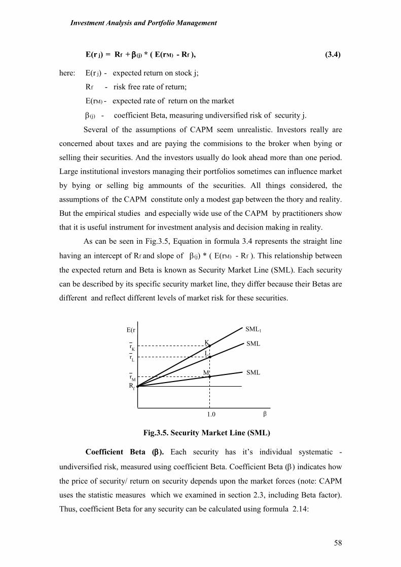
Investment Analysis and Portfolio Management
58
E(r j) = Rf + ββββ(j) * ( E(rM) - Rf ), (3.4)
here: E(r j) - expected return on stock j;
Rf - risk free rate of return;
E(rM) - expected rate of return on the market
β(j) - coefficient Beta, measuring undiversified risk of security j.
Several of the assumptions of CAPM seem unrealistic. Investors really are
concerned about taxes and are paying the commisions to the broker when bying or
selling their securities. And the investors usually do look ahead more than one period.
Large institutional investors managing their portfolios sometimes can influence market
by bying or selling big ammounts of the securities. All things considered, the
assumptions of the CAPM constitute only a modest gap between the thory and reality.
But the empirical studies and especially wide use of the CAPM by practitioners show
that it is useful instrument for investment analysis and decision making in reality.
As can be seen in Fig.3.5, Equation in formula 3.4 represents the straight line
having an intercept of Rf and slope of β(j) * ( E(rM) - Rf ). This relationship between
the expected return and Beta is known as Security Market Line (SML). Each security
can be described by its specific security market line, they differ because their Betas are
different and reflect different levels of market risk for these securities.
Fig.3.5. Security Market Line (SML)
Coefficient Beta (ββββ). Each security has it’s individual systematic -
undiversified risk, measured using coefficient Beta. Coefficient Beta (β) indicates how
the price of security/ return on security depends upon the market forces (note: CAPM
uses the statistic measures which we examined in section 2.3, including Beta factor).
Thus, coefficient Beta for any security can be calculated using formula 2.14:
K
M
L
1.0
E(r
)
R
f
β
SML
SML1
SML
r
L
r
K
r
M
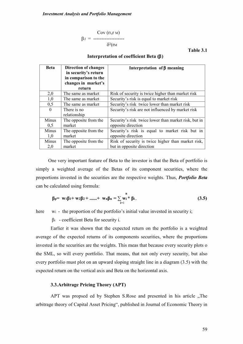
Investment Analysis and Portfolio Management
59
Cov (rJ,r M)
βJ = -------------------
δ²(rM
Table 3.1
Interpretation of coefficient Beta (ββββ)
Beta Direction of changes in security’s return
in comparison to the changes in market’s
return
Interpretation of ββββ meaning
2,0 The same as market Risk of security is twice higher than market risk
1,0 The same as market Security’s risk is equal to market risk
0,5 The same as market Security’s risk twice lower than market risk
0 There is no
relationship Security’s risk are not influenced by market risk
Minus
0,5
The opposite from the
market Security’s risk twice lower than market risk, but in
opposite direction
Minus
1,0 The opposite from the
market Security’s risk is equal to market risk but in
opposite direction
Minus
2,0
The opposite from the
market Risk of security is twice higher than market risk,
but in opposite direction
One very important feature of Beta to the investor is that the Beta of portfolio is
simply a weighted average of the Betas of its component securities, where the
proportions invested in the securities are the respective weights. Thus, Portfolio Beta
can be calculated using formula:
n
βp= w1β1+ w2β2 + ......+ wnβn = ∑ wi * βi , (3.5) i=1
here wi - the proportion of the portfolio’s initial value invested in security i;
βi - coefficient Beta for security i.
Earlier it was shown that the expected return on the portfolio is a weighted
average of the expected returns of its components securities, where the proportions
invested in the securities are the weights. This meas that because every security plots o
the SML, so will every portfolio. That means, that not only every security, but also
every portfolio must plot on an upward sloping straight line in a diagram (3.5) with the
expected return on the vertical axis and Beta on the horizontal axis.
3.3.Arbitrage Pricing Theory (APT)
APT was propsed ed by Stephen S.Rose and presented in his article „The
arbitrage theory of Capital Asset Pricing“, published in Journal of Economic Theory in
Investment Analysis and Portfolio Management
60
1976. Still there is a potential for it and it may sometimes displace the CAPM. In the
CAPM returns on individual assets are related to returns on the market as a whole. The
key point behind APT is the rational statement that the market return is determined by
a number of different factors. These factors can be fundamental factors or statistical. If
these factors are essential, there to be no arbitrage opportunities there must be
restrictions on the investment process. Here arbitrage we understand as the earning of
riskless profit by taking advantage of differential pricing for the same assets or
security. Arbitrage is is widely applied investment tactic.
APT states, that the expected rate of return of security J is the linear function
from the complex economic factors common to all securities and can be estimated
using formula:
E(rJ) = E(ŕJ) + β1J I1J + β2J I2J + ... + βnJ InJ + εJ , (3.6)
here: E(rJ) - expected return on stock J;
E(ŕJ) - expected rate of return for security J, if the influence of all factors is
0;
IiJ - the change in the rate of return for security J, influenced by economic
factor i (i = 1, ..., n);
βiJ - coefficient Beta, showing sensitivity of security’s J rate of return
upon the factor i (this influence could be both positive or negative);
εJ - error of rounding for the security J (expected value – 0).
It is important to note that the arbitrage in the APT is only approximate,
relating diversified portfolios, on assumption that the asset unsystematic (specific)
risks are negligable compared with the factor risks.
There could presumably be an infinitive number of factors, although the
empirical research done by S.Ross together with R. Roll (1984) identified four factors
– economic variables, to which assets having even the same CAPM Beta, are
differently sensitive:
• inflation;
• industrial production;
• risk premiums;
• slope of the term structure in interst rates.
Investment Analysis and Portfolio Management
61
In practice an investor can choose the macroeconomic factors which seems
important and related with the expected returns of the particular asset. The examples
of possible macroeconomic factors which could be included in using APT model :
• GDP growth;
• an interest rate;
• an exchange rate;
• a defaul spread on corporate bonds, etc.
Including more factors in APT model seems logical. The institutional investors
and analysts closely watch macroeconomic statistics such as the money supply,
inflation, interest rates, unemployment, changes in GDP, political events and many
others. Reason for this might be their belief that new information about the changes in
these macroeconomic indicators will influence future asset price movements. But it is
important to point out that not all investors or analysts are concerned with the same set
of economic information and they differently assess the importance of various
macroeconomic factors to the assets they have invested already or are going to invest.
At the same time the large number of the factors in the APT model would be
impractical, because the models seldom are 100 percent accurate and the asset prices
are function of both macroeconomic factors and noise. The noise is coming from
minor factors, with a little influence to the result – expected rate of return.
The APT does not require identification of the market portfolio, but it does
reguire the specification of the relevant macroeconomic factors. Much of the current
empirical APT research are focused on identification of these factors and the
determination of the factors’ Betas. And this problem is still unsolved. Although more
than two decades have passed since S. Ross introduced APT model, it has yet to reach
the practical application stage.
The CAPM and APT are not really essentially different, because they are
developed for determing an expected rate of return based on one factor (market
portfolio – CAPM) or a number of macroeconomic factors (APT). But both models
predict how the return on asset will result from factor sensitivities and this is of great
importance to the investor.
Investment Analysis and Portfolio Management
62
3.4. Market efficiency theory
The concept of market efficiency was proposed by Eugene Fama in 1965, when
his article “Random Walks in Stock Prices” was published in Financial Analyst
Journal.
Market efficiency means that the price which investor is paying for financial
asset (stock, bond, other security) fully reflects fair or true information about the
intrinsic value of this specific asset or fairly describe the value of the company – the
issuer of this security. The key term in the concept of the market efficiency is the
information available for investors trading in the market. It is stated that the market
price of stock reflects:
1. All known information, including:
� Past information, e.g., last year’s or last quarter’s, month’s
earnings;
� Current information as well as events, that have been announced but
are still forthcoming, e.g. shareholders’ meeting.
2. Information that can reasonably be inferred, for example, if many investors
believe that ECB will increase interest rate in the nearest future or the government
deficit increases, prices will reflect this belief before the actual event occurs.
Capital market is efficient, if the prices of securities which are traded in the
market, react to the changes of situation immediately, fully and credibly reflect all the
important information about the security’s future income and risk related with
generating this income.
What is the important information for the investor? From economic point of
view the important information is defined as such information which has direct
influence to the investor’s decisions seeking for his defined financial goals. Example,
the essential events in the joint stock company, published in the newspaper, etc.
Market efficiency requires thet the adjustment to new information occurs very
quikly as the information becomes known. Obvious, that Internet has made the markets
more efficient in the sense of how widely and quickly information is disseminated.
There are 3 forms of market efficiency under efficient market hypothesis:
• Weak form of efficiency;
• Semi- strong form of efficiency;
• Strong form of the efficiency.
Investment Analysis and Portfolio Management
63
Under the weak form of efficiency stock prices are assumed to reflect any
information that may be contained in the past history of the stock prices. So, if the
market is characterized by weak form of efficiency, no one investor or any group of
investors should be able to earn over the defined period of time abnormal rates of
return by using information about historical prices available for them and by using
technical analysis. Prices will respond to news, but if this news is random then price
changes will also be random.
Under the semi-strong form of efficiency all publicly available information is
presumed to be reflected in stocks’ prices. This information includes information in the
stock price series as well as information in the firm’s financial reports, the reports of
competing firms, announced information relating to the state of the economy and any
other publicly available information, relevant to the valuation of the firm. Note that
the market with a semi strong form of efficiency encompasies the weak form of the
hypothesis because the historical market data are part of the larger set of all publicly
available information. If the market is characterized by semi-strong form of efficiency,
no one investor or any group of investors should be able to earn over the defined
period of time abnormal rates of return by using information about historical prices
and publicly available fundamental information(such as financial statemants) and
fundamental analysis.
The strong form of efficiency which asserts that stock prices fully reflect all
information, including private or inside information, as well as that which is publicly
available. This form takes the notion of market efficiency to the ultimate extreme.
Under this form of market efficiency securities’ prices quickly adjust to reflect both
the inside and public information. If the market is characterized by strong form of
efficiency, no one investor or any group of investors should be able to earn over the
defined period of time abnormal rates of return by using all information available for
them.
The validity of the market efficiency hypothesis whichever form is of great
importance to the investors because it determines whether anyone can outperform the
market, or whether the successful investing is all about luck. Efficient market
hypothesis does not require to behave rationally, only that in response to information
there will be a sufficiently large random reaction that an excess profit cannot be made.
Investment Analysis and Portfolio Management
64
The concept of the market efficiency now is criticezed by some market analysts
and participants by stating that no one market can be fully efficient as some irrational
behavior of investors in the market occurs which is more based on their emotions and
other psychological factors than on the information available (the psychological
aspects of investment decision making will be disscussed further, in chapter 6). But, at
the same time, it can be shown that the efficient market can exist, if in the real markets
following events occur:
� A large number of rational, profit maximizing investors exist who are
actively and continuously analyzing valuing and trading securities;
� Information is widely available to market participants at the same time
and without or very small cost;
� Information is generated in a random walk manner and can be treated as
independent;
� Investors react to the new information quickly and fully, though causing
market prices to adjust accordingly.
Summary
1. Essentiality of the Markowitz portfolio theory is the problem of optimal portfolio
selection. The Markowitz approach included portfolio formation by considering
the expected rate of return and risk of individual stocks measured as standard
deviation, and their interrelationship as measured by correlation. The
diversification plays a key role in the modern portfolio theory.
2. Indifference curves represent an investor’s preferences for risk and return. These
curves should be drawn, putting the investment return on the vertical axis and the
risk on the horizontal axis.
3. Two important fundamental assumptions than applying indifference curves to
Markowitz portfolio theory. An assumption of nonsatiation assumes that the
investors prefer higher levels of return to lower levels of return, because the
higher levels of return allow the investor to spend more on consumption at the
end of the investment period. An assumption of risk aversion assumes that the
investor when given the choise, will choose the investment or investment
portfolio with the smaller risk, i.e. the investors are risk averse.
Investment Analysis and Portfolio Management
65
4. Efficient set theorem states that an investor will choose his/ her optimal portfolio
from the set of the portfolios that (1) offer maximum expected return for varying
level of risk, and (2) offer minimum risk for varying levels of expected return.
5. Efficient set of portfolios involves the portfolios that the investor will find
optimal ones. These portfolios are lying on the “northwest boundary” of the
feasible set and is called an efficient frontier. The efficient frontier can be
described by the curve in the risk-return space with the highest expected rates of
return for each level of risk. Feasible set is opportunity set, from which the
efficient set of portfolio can be identified. The feasibility set represents all
portfolios that could be formed from the number of securities and lie either or or
within the boundary of the feasible set.
6. Capital Market Line (CML) shows the trade off-between expected rate of return
and risk for the efficient portfolios under determined risk free return.
7. The expected rate of return on the portfolio is the weighted average of the
expected returns on its component securities.
8. The calculation of standard deviation for the portfolio can‘t simply use the
weighted average approach. The reason is that the relationship between the
securities in the same portfolio measured by coefficient of correlation must be
taken into account. When forming the diversified portfolios consisting large
number of securities investors found the calculation of the portfolio risk using
standard deviation technically complicated.
9. Measuring Risk in Capital asset Pricing Model (CAPM) is based on the
identification of two key components of total risk: systematic risk and
unsystematic risk. Systematic risk is that associated with the market.
Unsystematic risk is unique to an individual asset and can be diversified away by
holding many different assets in the portfolio. In CAPM investors are
compensated for taking only systematic risk.
10. The essence of the CAPM: CAPM predicts what an expected rate of return for
the investor should be, given other statistics about the expected rate of return in
the market, risk free rate of return and market risk (systematic risk).
11. Each security has it’s individual systematic - undiversified risk, measured using
coefficient Beta. Coefficient Beta (β) indicates how the price of security/ return
on security depends upon the market forces. The Beta of the portfolio is simply a
Investment Analysis and Portfolio Management
66
weighted average of the Betas of its component securities, where the proportions
invested in the securities are the respective weights.
12. Security Market Line (SML) demonstrates the relationship between the expected
return and Beta. Each security can be described by its specific security market
line, they differ because their Betas are different and reflect different levels of
market risk for these securities.
13. Arbitrage Pricing Theory (APT) states, that the expected rate of return of security
is the linear function from the complex economic factors common to all
securities. There could presumably be an infinitive number of factors. The
examples of possible macroeconomic factors which could be included in using
APT model are GDP growth; an interest rate; an exchange rate; a defaul spread
on corporate bonds, etc.
14. Market efficiency means that the price which investor is paying for financial
asset (stock, bond, other security) fully reflects fair or true information about the
intrinsic value of this specific asset or fairly describe the value of the company –
the issuer of this security. The key term in the concept of the market efficiency is
the information available for investors trading in the market.
15. There are 3 forms of market efficiency under efficient market hypothesis: weak
form of efficiency; semi- strong form of efficiency; strong form of the
efficiency.Under the weak form of efficiency stock prices are assumed to reflect
any information that may be contained in the past history of the stock
prices.Under the semi-strong form of efficiency all publicly available information
is presumed to be reflected in stocks’ prices.The strong form of efficiency which
asserts that stock prices fully reflect all information, including private or inside
information, as well as that which is publicly available.
Key-terms
• Arbitrage
• Arbitrage Pricing Theory
• (APT)
• Coefficient Beta (β)
• Capital Market Line (CML)
• Capital Asset Pricing Model
• (CAPM)
• Efficient frontier
• Efficient set of portfolios
• Expected rate of return of the
portfolio
• Feasible set
• Indifference curves
• Map of Indiference Curves
Investment Analysis and Portfolio Management
67
• Market efficiency
• Markowitz Portfolio Theory
• Market Portfolio
• Nonsatiation
• Portfolio Beta
• Risk aversion
• Risk free rate of return
• Risk of the portfolio
• Security Market Line (SML)
• Systematic risk
• Standard deviation of the
• portfolio
• Semi- strong form of market
• efficiency
• Strong form of market
• efficiency
• Total risk
• Unsystematic (specific) risk
• Weak form of market
efficiency
Questions and problems
1. Explain why most investors prefer to hold a diversified portfolio of securities as
opposed to placing all of their wealth in a single asset.
2. In terms of the Markowitz portfolio model, explain, how an investor identify his /
her optimal portfolio. What specific information does an investor need to identify
optimal portfolio?
3. How many portfolios are on an efficient frontier? How is an investor’s risk
aversion indicated in an indiference curve?
4. Describe the key assumptions underlying CAPM.
5. Many of underlyong assumptions of the CAPM are violated in some degree in
“real world”. Does that fact invalidate model’s calculations? Explain.
6. If the risk-free rate of return is 6% and the return on the market portfolio is 10%,
what is the expected return on an asset having a Beta of 1,4, according to the
CAPM?
7. Under the CAPM, at what common point do the security market lines of individual
stocks intersect?
8. Given the following information:
• Expected return for stock A = 18%
• Expected return for stock B = 25%
• Standartd deviation of stock A = 12%
• Standard deviation of stock B = 20%
• Correlation coefficient = 1,0.
Choose the investment below that represents the minimum risk portfolio:
Investment Analysis and Portfolio Management
68
a) 100% invest in stock A;
b) 100% invest in stock B;
c) 50% in stock A and 50% in stock B;
d) 20% invest in stock A and 80% in stock B
e) 60% invest in stock A and 40% in stock B.
9. The following investment portfolios are evaluated by investor:
Portfolio Expected rate of
return, %
Standard
deviation
A 12 15
B 10 8
C 10 9
Using Markowitz portfolio theory explain the choise for investor between
portfolios A,B and C.
10. Investor owns the portfolio composed of three stocks.The Betas of these stocks
and their proportions in portfolio are shown in the table. What is the Beta of the
investor’s portfolio?
Stock Beta Proportion in
portfolio, % A 0,8 30
B 1,2 40
C -0,9 30
11. How does the CAPM differs from the APT model?
12. Comment on the risk of the stocks presented below. Which of them are more /less
risky and why?
Stock Beta
A 0,92
B 2,20
C 0,97
D -1.12
E 1.18
F 0,51
13. What is meant by an efficient market? What are the benefits to the economy from
an efficient market?
14. If the efficient market hypothesis is true, what are the implications for the
investors?
Investment Analysis and Portfolio Management
69
15. What are the conditions for an efficient market? Discuss if are they met in the
reality.
16. If stock’s prices are assumed to reflect any information that may be contained in
the past history of the stock price itself, this is
a) Strong form of efficiency;
b) Semi-strong form of efficiency;
c) Weak form of efficiency;
d) Not enough information to determine form of efficiency.
17. Investor ownes a portfolio of four securities. The characteristics of the securities
and their proportions in the portfolio are presented in the table.
Security Coefficient Beta Proportion, % Expected rate
of return, %
A 1,40 30 13
B 0,90 30 18
C 1,00 20 10
D -1,30 20 12
a) What is the expected rate of return of this portfolio?
b) What is the risk of the portfolio?
c) If the investor wants to reduce risk in his portfolio how he could
restructure his portfolio?
18. The following table presents the three-stock portfolio.
Stocks Portfolio
Weight
Coefficient
Beta
Expected
return
Standard
deviation
A 0,25 0,50 0,40 0,07
B 0,25 0,50 0,25 0,05
C 0,50 1,00 0,21 0,07
Variance of the market returns is 0,06.
a) What is the Beta coefficient of the portfolio?
b) What is the expected rate of return on the portfolio?
c) What is an actual variance of the portfolio, if the following actual
covariance between the stock’s returns is given:
Cov (rA, rB) = 0,020
Cov (rA, rC) = 0,035
Cov (rB, rC) = 0,035
Investment Analysis and Portfolio Management
70
References and further readings
1. Fama, Eugene (1965). Random Walks in Stock Prices. // Financial Analysts
Journal, September.
2. Fama, Eugene (1970).Efficient Capital Markets: A Review of Theory and
Empirical Work// Journal of Business.
3. Haugen, Robert A. (2010). The New Finance. 4th
ed. Prentice Hall.
4. Haugen, Robert A. (2001). Modern Investment Theory. 5th
ed. Prentice Hall.
5. Jones, Charles P.(2010).Investments Principles and Concepts. JohnWiley & Sons,
Inc.
6. Markowitz, Harry. (1952). Portfolio Selection. // Journal of Finance,7(1), p. 77-91.
7. Sharpe, William F. (1964). Capital Assets Prices: A Theory of Market Equilibrium
under Conditions of Risk // Journal of Finance, 19 (3), p. 425-442.
8. Sharpe, William F., Gordon J.Alexander, Jeffery V.Bailey. (1999). Investments.
International edition. Prentice –Hall International.
9. Strong, Robert A. (1993). Portfolio Construction, Management and Protection.
Investment Analysis and Portfolio Management
71
4. Investment in Stocks
Mini-contents
4.1. Stock as specific investment.
4.2. Stock analysis for investment decision making.
4.2.3.E-I-C analysis.
4.2.4.Fundamental analysis.
4.3. Decision making of investment in stocks. Stock. valuation
4.4. Formation of stock portfolios.
4.5. Strategies for investing in stocks.
Summary
Key terms
Questions and problems
References and further readings
Relevant websites
4.1. Stock as specific investment
Stock represents part ownership in a firm.
2 main types of stock (see Chapter 1)
• Common stock
• Preferred stock
In this chapter we focus only on the investment in common stocks.
Common stock = Common share = Equity
The main features of the common stock:
• Typically each common stock owned entitles an investor to one vote in
corporate shareholders’ meeting.
• Investor receives benefits in the form of dividends, capital gains or both.
But:
� dividends are paid to shareholders only after other liabilities such as
interest payments have been settled;
� typically the firm does not pay all its earnings in cash dividends;
� special form of dividend is stock dividend, in which the corporation
pays in stocks rather than cash.
• Common stock has no stated maturity. Common stock does not have a date
on which the corporation must buy it back. But: some corporations pay
cash to their shareholders by purchasing their own shares. These are known
as share buybacks.
Investment Analysis and Portfolio Management
72
• Common stocks on the whole historically have provided a higher return,
but they also have higher risk. An investor earns capital gains (the
difference between the purchase price and selling price) when he / she sell
at a higher price than the purchase price.
Main advantages of common stock as investment:
• the investment income is usually higher;
• the investor can receive operating income in cash dividends;
• common stock has a very high liquidity and can easily be moved from one
investor to the other;
• the costs of transaction with common stocks involved are relatively low;
• the nominal price of common stock is lower in comparison with the other
securities.
Main disadvantages of common stock as investment:
• common stock is more risky in comparison with many other types of
securities;
• the selection of these securities is complicated: high supply and difficult to
evaluate;
• the operating income is relatively low (the main income is received from
the capital gain – change in stock price).
4.2.Stock analysis for investment decision making
In this section the focus is on the fundamental analysis of common stocks.
Although technical analysis is used by many investors, fundamental analysis is far
more prevalent. By performing fundamental analysis investor forecasts among other
things, the future changes in GDP, changes sales, other performance indicators for a
number of industries and, in particular, future sales, earnings for a number of the
firms. The main objective of this analysis for investor is to identify the attractive
potential investments in stocks.
Analysts and investors use two alternative approaches for fundamental
analysis:
• “Top-down” forecasting approach;
• “Bottom-up” forecasting approach.
Using “top-down” forecasting approach the investors are first involved in
making the analysis and forecast of the economy, then for industries, and finally for
Investment Analysis and Portfolio Management
73
companies. The industry forecasts are based on the forecasts for the economy and a
company’s forecasts are based on the forecasts for both its industry and the economy.
Using “bottom-up”forecasting approach, the investors start with the analysis
and forecast for companies, then made analysis and forecasts for industries and for the
economy.
In practice “top down” approach prevail in analysis and forecasting because
logically for forecasting of the companies performance the changes in macroeconomic
environment must be analyzed first otherwise the inconsistent assumptions could be
drawn. The combination of two approaches is used by analysts too. For example,
analysis and forecasts are made for the economy using “top-down” approach and then
using “bottom-up” approach continuing with the forecasts for individual companies.
But despite of the different approaches to the sequence of the analysis the content of it
is based on the E-I-C analysis.
4.2.1. E-I-C analysis
E-I-C analysis includes:
� E - Economic (macroeconomic) analysis (describes the
macroeconomic situation in the particular country and its potential
influence on the profitability of stocks).
� I - Industry analysis (evaluates the situation in the particular industry/
economic sector and its potential influence on the profitability of
stocks).
� C - Company analysis (the financial analysis of the individual
companies from the shareholder approach)
The contents of Macroeconomic analysis:
• The behavior of economics in the context of economic cycle (at what
point of this cycle is the economy now: growth stage? peak? decline
stage? recession stage?);
• Fiscal policy of the government (financial stability, budget deficit,
public debt, etc.)
• Monetary policy (the stability of national currency against other foreign
currencies; the ability of authorities (Central Bank) to use the money
market instruments on time, etc.);
Investment Analysis and Portfolio Management
74
• the other economic factors:
� inflation/deflation;
� the level of unemployment;
� the level of consumption;
� investments into businesses;
� the possibilities to use different types of energy, their prices;
� foreign trade and the exchange rate of the foreign currency
against national currency (devaluation? revaluation?)
The contents of Industry analysis could be disclosed answering following
questions:
• What is the nature of the industry? Is it monopolistic or competitive?
• What is the level of regulation and administration inside this industry?
• What is the situation with the self-organization of the human resources
in this industry? Is where any unions other organized structures?
• How important and how complex is the technology for this industry?
• What are the key factors which influence this industry?
• What conditions in production and financial activity are important in
this industry?
• (production resources, the perspectives for raising capital, competition
form the other countries, etc.)
• What is the stage of the industry’s development cycle? (Introductory?
Growth? Maturity? Decline?)
The other way for the development of Industry’s analysis by focusing it into
four important areas:
I. Demand:
• Could this sector/ industry be described as growing, mature or
cyclical?
• How are this sector/ industry influenced by changes in GDP or
interest rates?
• If the industry is cyclical, what is the key driver of it demand/ profit:
business (capital expenditures) or consumption cycle?
• How precisely the demand for capital expenditures is defined?

Investment Analysis and Portfolio Management
75
• Are the goods in this industry expensive? luxury goods? cheap? For
day-to-day consumption?
II. Pricing:
• How consolidated (concentrated) is this industry?
• What are the barriers for entrance to this industry? Are they high?
• How powerful and demanding are the consumers in this industry?
• Is where in the market of industry’s goods the surplus, how strong is
the fight for market share?
• Is where in this industry a high competition in the international
environment?
III. Costs:
• How is the industry supplied with the implements of production?
• Are the tendencies of the prices for raw materials used in this
industry substantially influencing the profit?
• Are the labor costs the main component?
• Is the question of qualification for the human resources in this
industry?
IV. The influence of the whole economics and financial market to the
industry:
• Is this industry defensive or growing? How it could function in
period of economic recession?
• How is this industry influenced by interest rates?
• Are severe stocks dominated in this industry?
• Is this sector global?
• How the fluctuations in currency exchange rate are influencing the
sector? Are these fluctuations of currency exchange rate influencing
the amount of profit received from abroad or the competitiveness of
the sector?
• Is it possibility that political and/ or regulation risk could influence
the sector?
4.2.2. Fundamental analysis
The base for the company analysis is fundamental analyses are the publicly
disclosed and audited financial statements of the company:
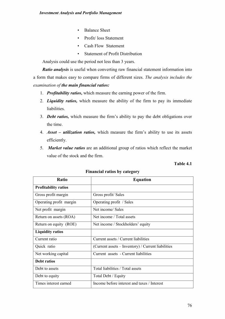
Investment Analysis and Portfolio Management
76
• Balance Sheet
• Profit/ loss Statement
• Cash Flow Statement
• Statement of Profit Distribution
Analysis could use the period not less than 3 years.
Ratio analysis is useful when converting raw financial statement information into
a form that makes easy to compare firms of different sizes. The analysis includes the
examination of the main financial ratios:
1. Profitability ratios, which measure the earning power of the firm.
2. Liquidity ratios, which measure the ability of the firm to pay its immediate
liabilities.
3. Debt ratios, which measure the firm’s ability to pay the debt obligations over
the time.
4. Asset – utilization ratios, which measure the firm’s ability to use its assets
efficiently.
5. Market value ratios are an additional group of ratios which reflect the market
value of the stock and the firm.
Table 4.1
Financial ratios by category
Ratio Equation
Profitability ratios
Gross profit margin Gross profit/ Sales
Operating profit margin Operating profit / Sales
Net profit margin Net income/ Sales
Return on assets (ROA) Net income / Total assets
Return on equity (ROE) Net income / Stockholders’ equity
Liquidity ratios
Current ratio Current assets / Current liabilities
Quick ratio (Current assets – Inventory) / Current liabilities
Net working capital Current assets - Current liabilities
Debt ratios
Debt to assets Total liabilities / Total assets
Debt to equity Total Debt / Equity
Times interest earned Income before interest and taxes / Interest
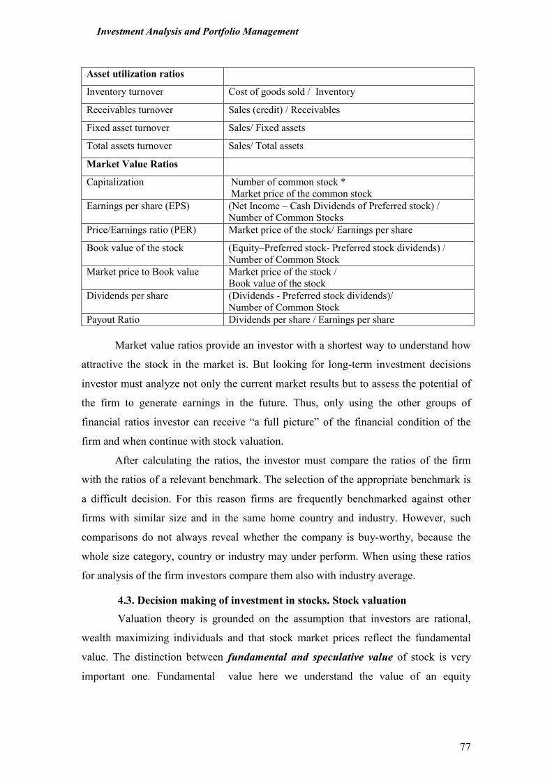
Investment Analysis and Portfolio Management
77
Asset utilization ratios
Inventory turnover Cost of goods sold / Inventory
Receivables turnover Sales (credit) / Receivables
Fixed asset turnover Sales/ Fixed assets
Total assets turnover Sales/ Total assets
Market Value Ratios
Capitalization Number of common stock *
Market price of the common stock
Earnings per share (EPS) (Net Income – Cash Dividends of Preferred stock) /
Number of Common Stocks
Price/Earnings ratio (PER) Market price of the stock/ Earnings per share
Book value of the stock (Equity–Preferred stock- Preferred stock dividends) /
Number of Common Stock
Market price to Book value Market price of the stock /
Book value of the stock
Dividends per share (Dividends - Preferred stock dividends)/
Number of Common Stock
Payout Ratio Dividends per share / Earnings per share
Market value ratios provide an investor with a shortest way to understand how
attractive the stock in the market is. But looking for long-term investment decisions
investor must analyze not only the current market results but to assess the potential of
the firm to generate earnings in the future. Thus, only using the other groups of
financial ratios investor can receive “a full picture” of the financial condition of the
firm and when continue with stock valuation.
After calculating the ratios, the investor must compare the ratios of the firm
with the ratios of a relevant benchmark. The selection of the appropriate benchmark is
a difficult decision. For this reason firms are frequently benchmarked against other
firms with similar size and in the same home country and industry. However, such
comparisons do not always reveal whether the company is buy-worthy, because the
whole size category, country or industry may under perform. When using these ratios
for analysis of the firm investors compare them also with industry average.
4.3. Decision making of investment in stocks. Stock valuation
Valuation theory is grounded on the assumption that investors are rational,
wealth maximizing individuals and that stock market prices reflect the fundamental
value. The distinction between fundamental and speculative value of stock is very
important one. Fundamental value here we understand the value of an equity
Investment Analysis and Portfolio Management
78
investment that is held over the long term, as opposed to the value that can be realized
by short term, speculative trading.
Stock valuation process:
1. Forecasting of future cash flows for the stock.
2. Forecasting of the stock price.
3. Calculation of Present value of these cash flows. This result is intrinsic
(investment) value of stock.
4. Comparison of intrinsic value of stock and current market price of the stock
and decision making: to buy or to sell the stock.
Valuation methods:
1. Method of income capitalization.
2. Discounted dividend models.
3. Valuation using multiples.
Method of income capitalization
This method is based on the use of Present and Future value concept well
known in finance. The value of any investment could be estimated as present value of
future cash flows generated by this investment, using formula:
V = CF1 / (1 + k) + CF2/ (1 + k)² + … + CFn / (1 + k)ⁿ =
= ΣCFt/ (1 + k)t (4.1)
here CF - expected cash flows from the investment during period t;
k - discount rate (capitalization rate or required rate of return for the
investor, which include the expected level of risk).
Discounted dividend models
The discounted dividends models (DDM) is based on the method of income
capitalization and considers the stock price as the discounted value of future dividends,
at the risk adjusted required return of equity, for dividend paying firms.
Important assumption behind the DDM: the only way a corporation can
transfer wealth to its stockholders is through the payment of dividend, because
dividends are the only source of cash payment to a common stock investor.
Common stock value using DDM:
V = D1 /(1 + k) + D2 / (1 + k)² + … + Dn/(1 + k)ⁿ = Σ Dt / (1 + k)t , (4.2)
Investment Analysis and Portfolio Management
79
here D1,2 …,t is stock dividend for the period t.
The forecasted dividends during long-term valuation period of dividends are
the key factor influencing the stock value. Expected growth rate in dividends (g) is
calculated by formula:
g = (Dt - Dt-1)/ Dt-1 (4.3)
Various types of DDM, depending upon the assumptions about the expected
growth rate in dividends (g):
� “Zero” growth DDM
� Constant growth DDM
� Multistage growth DDM
“Zero” growth DDM
Assumption: D1 = D2 = D3 = ... = D∞, that means Dt = Dt-1 and g = 0.
The basic DDM formula for stock valuation using “zero” growth model
becomes as follows:
V = D1/ k or D0 / k0 (4.4)
Constant growth DDM
Assumption: if last year (t0) firm was paying D0 dividends, then in period t=1 its
dividends will grow at growth rate g:
D1 = D0 (1 + g) or Dt = Dt-1 (1 + g) = D0(1 + g)
The basic DDM formula for stock valuation using constant growth model
becomes as follows:
∞ V = ∑ D0 (1 + g)/ (1 + k)t (continuing series) (4.5) t = 1 or
V = D1/ (k - g) (Gordon formula) (4.6)
Multistage growth DDM
Assumption: after some defined period in the future T dividends expected each
year will grow at the constant growth rate g. Dividends before period T (D1, D2, D3,..
Investment Analysis and Portfolio Management
80
Dt) are forecasted individually. Investor individually defines then the period T will
start.
Future dividend cash flows for the stock, using this model:
T
before period T: VT1 = Σ Dt / (1 + k )t;
t=1
after period T : VT2 = DT + 1 / ( k – g ) ( 1 + k )T
Stock value using multistage growth method:
T
V = VT1 + VT2 = Σ Dt / (1 + k )t + D T+1 /( k – g ) ( 1 + k )T
(4.7) t=1
Valuation, when the stock keeping period is fixed
Example for 1 year:
V = (D1 + P1) / (1 + k) = + P1 / (1 + k) , (4.8)
here P1 - selling price for the stock after 1 year:
P1 = D2 / ( 1 + k ) + D3 / ( 1 + k )² + … + Dt / ( 1 + k )
t-1
And value of the stock will be:
V = D1 / (1 + k) + [D2 / ( 1 + k ) + D3 / ( 1 + k )² + … + Dt / ( 1 + k )
t-1] / (1 + k) =
N
= ∑ Dt / (1 + k) t (DDM basic formula, see 4.2) t=1
Decisions for the investor in stocks:
� If Pm < V - decision to buy the stock, because it is under valuated;
� If Pm > V - decision to sell the stock, because it is over valuated;
� If Pm = V - stock is valuated at the same range as in the market and
its current market price shows the intrinsic value.
Valuation using multiples
Practitioners value stock price using multiples.
The most common used multiply is the Price Earning Ratio (PER):
PER = P / EPS, (4.9)
here: P – market price of the stock;
Investment Analysis and Portfolio Management
81
EPS - earnings per share
Given PER and EPS, price
P = PER x EPS (4.10)
Observed PER. Prices of stock and earnings measures, from which observed
PERs are derived, are publicly available. Earnings per share are observed or estimates
of analysts. The observed PERs for a firm, a group of firms, an industry, of the index
derives directly from such data. What should be the PER, according to analysts, might
differ from observed PER. It is important to make a distinction between observed PER
with normative PER*, or what the PER should be.
PER* = V / EPS0 , (4.11)
here: PER* - normative PER
V - intrinsic value of the stock;
EPS0 - earnings per share for the last period.
Investor might consider that the PER* that should apply to the firm, of which
stock value has to be estimated, should be in line with peer firms selected or the
industry average.
Decision making for investment in stocks, using PER:
� If PER* > PER - decision to buy or to keep the stock, because it is
under valuated;
� If PER* < PER - decision to sell the stock, because it is over valuated;
� If PER* = PER - stock is valuated at the same range as in the market. In
this case the decision depends on the additional observations of investor.
There are remarkable variations of PERs across firms, industries, etc. This is
because PERs are a synthetic measure combining all effects of different equity value
drivers: growth, profitability, risk. PER is increasing, then the profitability of the firm
and its growth rates are increasing. PER is decreasing then the risk of the firm is
increasing. Interest rates are correlated with inverse of PER, because PER increases
when risk free rate decreases.
The other alternative multiples used for stock valuation by investors include:
• Sales / Market capitalization of the firm
• Sales / Equity value
• Market capitalization /Book Value of the Equity Ratio.
Investment Analysis and Portfolio Management
82
These alternative multiples are used when earnings are not representative.
Example could be the high growth (Internet) firms with negative net income, negative
EPS and actual stock price irrelevant usage.
When using these multiplies investors usually consider that the PER* that
should apply to the firm, of which stock value has to be estimated, should be in line
with peer firms selected or the industry average.
4.4. Formation of stock portfolios
In this section we review the important principles behind the stock selection
process that are relevant in the formation and management of the stock portfolios. We
focus on the explanation of the principal categories of common stock, especially the
investment characteristics that make a category of stock suitable for one portfolio but
not for another.
The most widely used categories of stocks are:
• blue chip stocks;
• income stocks;
• cyclical stocks;
• defensive stocks;
• growth stocks;
• speculative stocks;
• Penny stocks.
Blue chip stock is the best known of all the categories of stocks presented
above. These stocks represent the best-known firms among the investment community.
But it is difficult to define exactly this category of stock, because in most cases blue
chip stocks are presented using the examples of the firms. One common definition of
Blue Chip Company is that this company has long continuous history of divided
payments. For example, Coca Cola has a history of dividend payments more than for
100 years. But it doesn’t mean that the younger successful companies running business
for some decades and paying dividends can’t be categorized as “blue chips” in the
specific investment environment. From the other side, many high quality stocks do not
meet the criterion of uninterrupted dividend history. It is a practice that brokerage
firms recommend for their clients – individual investors the list of blue chip stock as
high quality ones in their understanding, based on the analysis of information about
the firm.
Investment Analysis and Portfolio Management
83
Income stocks are the stocks, the earnings of which are mainly in the form of
dividend income, as opposed to capital gains. It is considered a conservative,
dependable investment, suitable to supplement other income. Well-established
corporations with a consistent record of paying dividends are usually considered
income stock. In addition, income stocks usually are those that historically have paid a
larger-than-average percentage of their net income after taxes as dividends to their
shareholders and the payout ratio for these companies are high. The common examples
of income stocks are the stocks of public utilities, such as telecommunication
companies, electric companies, etc.
Cyclical stocks are the securities that go up and down in value with the trend
of business and economy, rising faster in the periods of rapidly improving business
conditions and sliding very noticeably when business conditions deteriorate. During a
recession they do poorly. The term cyclical does not imply that these stocks are more
predictable than other categories. They are cyclical because they follow business cycle.
The examples of cyclical stocks can be industrial chemicals, construction industry,
automobile producers, etc.
Defensive stocks (synonymous – protective stocks) are those which are
opposite to cyclical stocks. These stocks shift little in price movements and are very
rarely of interest to speculators. The defensive stocks have low Betas and thus are
assigned to the stocks with lower risk. Held by long-term investors seeking stability,
these stocks frequently withstand selling pressure in a falling market. The best
examples of defensive stocks are food companies, tobacco and alcohol companies and
utilities. Other defensive products include cosmetics, drugs, and health care products.
They continue to sell their products regardless of changes in macroeconomic
indicators.
Growth stocks (synonymous – performance stocks) are stocks of
corporations whose existing and projected earnings are sufficiently positive to indicate
an appreciable and constant increase in the stock’s market value over the extended
time period. The rate of increase in market value for these stocks is larger than those of
most corporate stock. Income stocks pay out a relatively high percentage of their
earnings as dividends, but growth stocks do not. Instead, the company reinvests its
earnings into profitable investment opportunities that are expected to increase the
value of the firm, and therefore, the value of the firm’s stock. Many firms have never
Investment Analysis and Portfolio Management
84
paid a dividend and publicly state they have no plans to do so. By default it seems
these should be a growth stocks, because a stock that pays no dividend and does not
increase in value would not be a very attractive investment. Though the analysts and
the experienced investors themselves spend the time trying to discover little-known
growth stocks.
Speculative stocks are the stocks issued by relatively new firms of unproven
financial status and by firms with less than average financial strength. Speculation, by
definition, involves a short time horizon, and the speculative stocks are those thet have
a potential to make their owners a lot of money quickly. At the same time, though,
they carry an unusually high degree of risk. Some analysts consider speculative stocks
to be a most risky growth stocks. However, some new established technological
companies that paid no dividends and had short history would probably be considered
a speculative rather than a growth stock.
Penny stocks are low-priced issues, often highly speculative, selling at very
small price a share. Thus, such stocks could be affordable even for the investors with
small amounts of money.
The categories of the stocks presented above are not really mutually exclusive.
As an examples show, some blue chip stocks at the same time can be an income stock.
Similarly, both cyclical and defensive stocks can be income stocks.
4.5. Strategies for investing in stocks
In this section we focus on the three main types of strategies than investing in
stocks:
• Sector rotation and business cycle strategy;
• Market timing strategy;
• Value screening strategy.
Sector rotation and business cycle strategy. The essentiality of this strategy:
each economic sector as potential investment object has the specific patterns of market
prices which depend upon the phase of the economic (business) cycle.
Sector rotation and business cycle strategy intends the movement of invested
funds from one sector to the other depending on the changes in the economic
(business) conditions.
This strategy use the classification of all stocks traded in the market on the
bases of their behavior in regard to business cycle. The following groups are identified:
Investment Analysis and Portfolio Management
85
� Defensive stocks
� Interest-sensitive stocks
� Consumer durables
� Capital goods
Defensive stocks were defined in the previous section (4.4). These stocks are
usually related with food industry, retail, tobacco, beverages industries,
pharmaceuticals and other suppliers of the necessity goods and services. The prices of
these stocks reach their highest levels in the later phases of business cycle.
Interest-sensitive stocks are related with the sectors of communications,
utilities, housing industry, also with the insurance and other financial institutions. The
behavior of these stocks is most unfavorable for the investor in the phase of economic
crises/ recession. These stocks are considered as a good investment in the early phases
of business cycle, i.e. in the optimistic phase.
Consumer durables are related with automobile, domestic electric appliances,
furniture industries, and luxury goods and also with the wholesale. These stocks are a
good investment in the middle of business cycle.
Capital goods are related with industries producing machinery, plant, office
equipment, computers and other electronic instruments. Because of the remarkable
time gap between the orders of this production and the terms of their realization, these
stocks demonstrate their high and stabile prices in the latest phases of business cycle.
Thus by knowing and identifying the different patterns of prices relating to
the industries in the real investment environment the investor can diversify his / her
stock portfolio which will reflect to the changes in the economic (business) cycle.
Market timing strategy. The essentiality of this strategy: the investors
endeavor to be „in-the-market“ when market is in a „bullish“ phase, i.e., when prices
are growing, and to withdraw from the market in the „bearish“ phase, i.e., when prices
are slumping.
Investors use several different techniques for forecasting the major ups and
downs in the market. The most often applied techniques using market timi9ng
strategies:
• Technical analysis;
• Stock valuation analysis
• Analysis of economic forecasting
Investment Analysis and Portfolio Management
86
Technical analysis is based on the diagrams of price fluctuations in the market, the
investors continuously watch the stocks which prices are growing and which falling
as they signalize about the presumable changes in the stock market.
The purpose of the stock valuation analysis is to examine whether the stock market is a
supply market, or is it a demand market. If the under valuated stocks prevail in the
market it reflects to supply market and vice versa – if the over valuated stocks prevail,
it reflects to demand market. The concept and key methods of stock valuation was
discussed in section 4.2. The valuation tools frequently used when applying for market
timing strategy are:
• Price/Earnings ratio (PER);
• The average market price/ book value ratio;
• The average dividend income.
Analysis of economic forecasting. Investors by forecasting changes in the macro
economy and in interest rates endeavor to decrease the investment in stocks in the
phases of economic downturn and to return to these investments during upturn phases
of the economy.
Valuation screening strategy. The essentiality of this strategy: by choosing
and applying one or combining several stock valuation methods and using available
information about the stocks from the data accumulated in the computer database, the
valuation screens are set by investor. All stocks on these screens are allocated on the
basis of their ratings in such an order: on the top of the screen – under valuated stocks,
at the bottom – over valuated stocks. Using these screens investors can form their
diversified stock portfolio and exercise the changes in the existent portfolio.
Various financial indicators and ratios can be used for the rating of stocks
when applying valuation screening strategy. The most often used are following
indicators:
• Price/Earnings ratio (PER);
• Dividend income
• Return on Equity (ROE)
• Return on Investments (ROI).
Valuation screening is very popular strategy; it is frequently used together
with the other investment strategies, because the investors in the market have
possibility to choose from the variety of stocks even in the same market segment.
Investment Analysis and Portfolio Management
87
What could be the best choose? – rating of the stocks as alternatives using the screen
can be the answer. Usually investors setting the screens combine more than one
indicator for rating of stocks searching for the better results in picking the stocks to
their portfolios. The examples of the other financial indicators used applying valuation
screening strategy:
• Return on assets (ROA)
• Net profit margin
• Debt to assets
• Debt to equity
• Earnings per share (EPS)
• Market price to Book value
Summary
1. Higher investment income, possibility to receive an operating income in cash
dividends, high liquidity and low costs of transactions are the main advantages of
investment in common stock.
2. The relatively higher risk in comparison with many other types securities, the
complicated selection of the stocks because of their high supply in the financial
market, the relatively low the operating income are the main disadvantages of
investment in common stock.
3. E-I-C analysis includes: Economic (macroeconomic) analysis, Industry analysis
and Company analysis. Two alternative approaches used for analysis: (1) “Top-
down” forecasting approach; (2) “Bottom-up” forecasting approach. Using “top-
down” forecasting approach the investors are first involved in making the analysis
and forecast of the economy, then for industries, and finally for companies. Using
“bottom-up” forecasting approach, the investors start with the analysis and forecast
for companies, then made analysis and forecasts for industries and for the
economy. The combination of two approaches is used by analysts too.
4. The Macroeconomic analysis includes the examining of economic cycle, fiscal
policy of the government, monetary policy, the other economic factors: inflation,
the level of unemployment; the level of consumption; investments into businesses;
the possibilities to use different types of energy, their prices; foreign trade and the
exchange rate, etc.
Investment Analysis and Portfolio Management
88
5. The Industry analysis includes the examining of the nature of the industry, the level
of regulation inside this industry, the situation with the self-organization of the
human resources the key factors which influence this industry (production
resources, the perspectives for raising capital, competition form the other countries,
etc), the stage of the industry’s development cycle. The alternative approach to the
industry analysis suggests the examining of four key areas: demand, pricing, costs
and the influence of the whole economics and financial markets.
6. The base for the company analysis is fundamental analysis is the publicly disclosed
and audited financial statements of the company: (Balance Sheet; Profit/ Loss
Statement; Cash Flow Statement; Statement of Profit Distribution). Analysis use
the period not less than 3 years.
7. Ratio analysis is useful when converting raw financial statement information into a
form that makes easy to compare firms of different sizes. This analysis includes the
examination of the main financial ratios: profitability ratios, which measure the
earning power of the firm; liquidity ratios, which measure the ability of the firm to
pay its immediate liabilities; debt ratios, which measure the firm’s ability to pay
the debt obligations over the time; asset – utilization ratios, which measure the
firm’s ability to use its assets efficiently and market value ratios are an additional
group of ratios which reflect the market value of the stock and the firm.
8. The investor must compare the ratios of the firm with the ratios of a relevant
benchmark. For this reason firms are frequently benchmarked against other firms
with similar size and in the same home country and industry.
9. Stock valuation process includes four stages: (1) forecasting of future cash flows
for the stock; (2) forecasting of the stock price; (3) calculation of Present value of
these cash flows. This result is intrinsic (investment) value of stock; (4)
comparison of and current and decision making: to buy or to sell the stock. If
market price of the stock is lower than intrinsic value of the stock decision would
be to buy the stock, because it is under valuated; if market price of the stock is
higher than intrinsic value of the stock decision would be to sell the stock, because
it is over valuated; if market price of the stock is equal to the intrinsic value of
stock is valuated at the same range as in the market and its current market price
shows the intrinsic value.
Investment Analysis and Portfolio Management
89
10. Most frequently used methods for valuation of common stocks are: the method of
income capitalization; discounted dividend models and valuation using multiples.
11. The discounted dividends models (DDM) are based on the method of income
capitalization and considers the stock price as the discounted value of future
dividends, at the risk adjusted required return of equity, for dividend paying firms.
Various types of DDM, depending upon the assumptions about the expected
growth rate in dividends (g):“Zero” growth DDM; Constant growth DDM;
Multistage growth DDM.
12. The most common used multiply is the Price Earning Ratio (PER). Decision
making for investment in stocks, using PER: if the normative PER is higher than
observed decision would be to buy or to keep the stock, because it is under
valuated; if the normative PER is lower than observed decision would be to sell the
stock, because it is over valuated; If normative and PER is equal to observed PER,
stock is valuated at the same range as in the market. In this case the decision
depends on the additional observations of investor.
13. The other alternative multiples used for stock valuation by investors include Sales /
Market capitalization of the firm; Sales / Equity value; Market capitalization /Book
Value of the Equity Ratio etc. These alternative multiples are used when earnings
are not representative.
14. The categories of stocks most widely used in the selection process and relevant in
the formation and management of the stock portfolios. are: blue chip stocks;
income stocks; cyclical stocks; defensive stocks; growth stocks; speculative stocks;
penny stocks.
15. Sector rotation and business cycle strategy intends the movement of invested funds
from one sector to the other depending on the changes in the economic (business)
conditions. This strategy use the classification of all stocks traded in the market on
the bases of their behavior in regard to business cycle.
16. The essentiality of market timing strategy is that the investors endeavor to be „in-
the-market“when market is in a „bullish“phase, i.e., when prices are growing, and
to withdraw from the market in the „bearish“phase, i.e., when prices are slumping.
17. Valuation screening strategy use the valuation screens set by investor. All stocks
on these screens are allocated on the basis of their ratings in such an order: on the
top of the screen – under valuated stocks, at the bottom – over valuated stocks.
Investment Analysis and Portfolio Management
90
Using these screens investors can form their diversified stock portfolio and
exercise the changes in the existent portfolio.
Key-terms
• Asset – utilization ratios
• Blue chip stocks
• “Bottom-up” forecasting
approach
• Capital goods
• Cyclical stocks
• Company analysis
• Constant growth DDM
• Consumer durables
• Debt ratios
• Defensive stocks
• Discounted dividend models
(DDM)
• Economic analysis
• E-I-C analysis
• Fundamental analysis
• Growth stocks
• Income stocks
• Income capitalization
• Industry analysis
• Interest-sensitive stocks
• Intrinsic (investment) value
• Liquidity ratios
• Market timing strategy
• Market value ratios
• Multiples method
• Multistage growth DDM
• Penny stocks
• Profitability ratios
• Sector rotation and business
cycle strategy
• Speculative stocks
• Stock valuation process
• Technical analysis
• “Top-down” forecasting
approach
• Value screening strategy
• “Zero” growth DDM
Questions and problems 1. The investor wants to identify if the stock of firm A is cyclical. How he/ she would
proceed?
2. Common stock hasn‘t term to maturity. How then can a stock that does not pay
dividends have any value? Give an examples of such firms listed in the domestic
market of your country.
3. What is the difference between blue chip and income stocks?
4. Give examples of defensive stocks in the domestic market of your country.
5. Present the examples of blue chip stocks in the domestic market Explain, why did
you categorize them as blue chips.
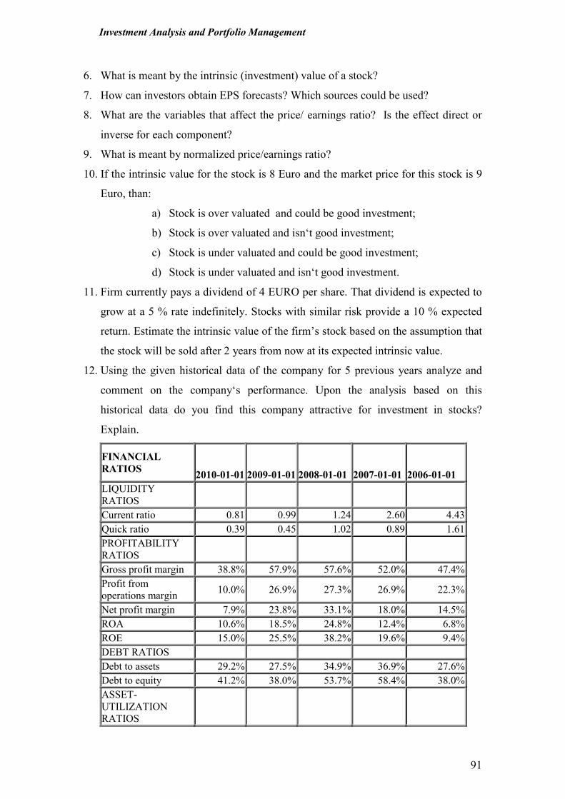
Investment Analysis and Portfolio Management
91
6. What is meant by the intrinsic (investment) value of a stock?
7. How can investors obtain EPS forecasts? Which sources could be used?
8. What are the variables that affect the price/ earnings ratio? Is the effect direct or
inverse for each component?
9. What is meant by normalized price/earnings ratio?
10. If the intrinsic value for the stock is 8 Euro and the market price for this stock is 9
Euro, than:
a) Stock is over valuated and could be good investment;
b) Stock is over valuated and isn‘t good investment;
c) Stock is under valuated and could be good investment;
d) Stock is under valuated and isn‘t good investment.
11. Firm currently pays a dividend of 4 EURO per share. That dividend is expected to
grow at a 5 % rate indefinitely. Stocks with similar risk provide a 10 % expected
return. Estimate the intrinsic value of the firm’s stock based on the assumption that
the stock will be sold after 2 years from now at its expected intrinsic value.
12. Using the given historical data of the company for 5 previous years analyze and
comment on the company‘s performance. Upon the analysis based on this
historical data do you find this company attractive for investment in stocks?
Explain.
FINANCIAL RATIOS
2010-01-01 2009-01-01
2008-01-01
2007-01-01
2006-01-01
LIQUIDITY
RATIOS
Current ratio 0.81 0.99 1.24 2.60 4.43
Quick ratio 0.39 0.45 1.02 0.89 1.61
PROFITABILITY
RATIOS
Gross profit margin 38.8% 57.9% 57.6% 52.0% 47.4%
Profit from
operations margin 10.0% 26.9% 27.3% 26.9% 22.3%
Net profit margin 7.9% 23.8% 33.1% 18.0% 14.5%
ROA 10.6% 18.5% 24.8% 12.4% 6.8%
ROE 15.0% 25.5% 38.2% 19.6% 9.4%
DEBT RATIOS
Debt to assets 29.2% 27.5% 34.9% 36.9% 27.6%
Debt to equity 41.2% 38.0% 53.7% 58.4% 38.0%
ASSET-
UTILIZATION
RATIOS
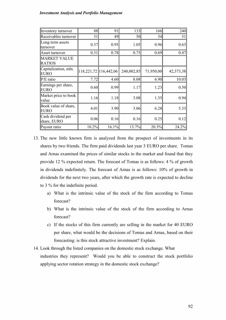
Investment Analysis and Portfolio Management
92
Inventory turnover 88 91 133 166 240
Receivables turnover 31 49 50 34 51
Long term assets
turnover 0.37 0.95 1.05 0.96 0.63
Asset turnover 0.31 0.78 0.75 0.69 0.47
MARKET VALUE
RATIOS
Capitalization, mln.
EURO 118,221,72 116,442,06 240,002,85 71,950,00 42,373,38
P/E ratio 7.72 4.60 8.08 6.90 10.03
Earnings per share,
EURO 0.60 0.99 1.17 1.23 0.50
Market price to book
value 1.16 1.18 3.08 1.35 0.94
Book value of share,
EURO 4.01 3.90 3.06 6.28 5.33
Cash dividend per
share, EURO 0.06 0.16 0.16 0.25 0.12
Payout ratio 10.2% 16.1% 13.7% 20.3% 24.2%
13. The new little known firm is analyzed from the prospect of investments in its
shares by two friends. The firm paid dividends last year 3 EURO per share. Tomas
and Arnas examined the prices of similar stocks in the market and found that they
provide 12 % expected return. The forecast of Tomas is as follows: 4 % of growth
in dividends indefinitely. The forecast of Arnas is as follows: 10% of growth in
dividends for the next two years, after which the growth rate is expected to decline
to 3 % for the indefinite period.
a) What is the intrinsic value of the stock of the firm according to Tomas
forecast?
b) What is the intrinsic value of the stock of the firm according to Arnas
forecast?
c) If the stocks of this firm currently are selling in the market for 40 EURO
per share, what would be the decisions of Tomas and Arnas, based on their
forecasting: is this stock attractive investment? Explain.
14. Look through the listed companies on the domestic stock exchange. What
industries they represent? Would you be able to construct the stock portfolio
applying sector rotation strategy in the domestic stock exchange?
Investment Analysis and Portfolio Management
93
References and further readings
1. Arnold, Glen (2010). Investing: the definitive companion to investment and the
financial markets. 2nd
ed. Financial Times/ Prentice Hall.
2. Barker, Richard (2001). Determining Value: Valuation Models and Financial
Statements. Financial Times / Prentice Hall.
3. Brammertz, Willi at al. (2009). Unified financial analysis. John Wiley & Sons, Ltd.
4. Fabozzi, Frank J. (1999). Investment Management. 2nd. ed. Prentice Hall Inc.
5. Francis, Jack C., Roger Ibbotson (2002). Investments: A Global Perspective.
Prentice Hall Inc.
6. Jones, Charles P. (2010). Investments Principles and Concepts. John Wiley &
Sons, Inc.
7. Rosenberg, Jerry M. (1993).Dictionary of Investing. John Wiley &Sons Inc.
8. Sharpe, William F., Gordon J.Alexander, Jeffery V.Bailey. (1999). Investments.
International edition. Prentice –Hall International.
9. Strong, Robert A. (1993). Portfolio Construction, Management and Protection.
10. Vause, B. (2009). Guide to Analyzing Companies. 5th
ed. The Economist Books/
Profile Books.
Relevant websites
http://www.marketwatch.com Market Watch
http://www.bloomberg.com Bloomberg
http://www.advfn.com ADVFN
http://www.zacks.com/screening Zaks Investment Research
http://www.reuters.com/ Reuters
www.nasdaqomx.com NASDAQ OMX
Investment Analysis and Portfolio Management
94
5. Investment in bonds
Mini-contents
5.1.Identification and classification of bonds
5.2.Bond analysis: structure and contents.
5.2.1. Quantitative analysis
5.2.2. Qualitative analysis
5.2.3. Market interest rates analysis
5.3.Decision making for investment in bonds. Bond valuation.
5.4.Strategies for investing in bonds. Immunization.
Summary
Key-terms
Questions and problems
References and further readings
Relevant websites
5.1. Identification and classification of bonds Bonds are securities with following basic characteristics:
• They are typically securities issued by a corporation or governmental body
for specified term: bonds become due for payment at maturity, when the
par value/ face value of bond are returned to the investors.
• Bonds usually pay fixed periodic interest installments, called coupon
payments. Some bonds pay variable income.
• When investor buys bond, he or she becomes a creditor of the issuer. Buyer
does not gain any kind of owner ship rights to the issuer, unlike in the case
with equity securities.
The main advantages of bonds to the investor:
• They are good source of current income;
• Investment to bonds is relatively safe from large losses;
• In case of default bondholders receive their payments before shareholders
can be compensated.
A major disadvantage of bonds is that potential profit from investment in bonds
is limited.
Currently in the financial markets there are a lot of various types of bonds and
investor must understand their differences and features before deciding what bonds
would be suitable for his/ her investment portfolio.
Investment Analysis and Portfolio Management
95
Bonds classification by their key features:
� By form of payment:
• Noninteresting bearing bonds - bonds issued at a discount. Throughout the
bond’s life its interest is not earned, however the bond is redeemed at
maturity for face value.
• Regular serial bonds - serial bonds in which all periodic installments of
principal repayment are equal in amount.
• Deferred –interest bonds –bonds paying interest at a later date;
• Income bonds – bonds on which interest is paid when and only when
earned by the issuing firm;
• Indexed bonds - bonds where the values of principal and the payout rise
with inflation or the value of the underlying commodity;
• Optional payment bonds – bonds that give the holder the choice to receive
payment on interest or principal or both in the currency of one or more
foreign countries, as well as in domestic currency.
� Coupon payment:
• Coupon bonds – bonds with interest coupons attached;
• Zero-coupon bonds – bonds sold at a deep discount from its face value and
redeemed at maturity for full face value. The difference between the cost of
the bond and its value when redeemed is the investor’s return. These
securities provide no interest payments to holders;
• Full coupon bonds – bonds with a coupon rate near or above current market
interest rate;
• Floating-rate bonds – debt instruments issued by large corporations and
financial organizations on which the interest rate is pegged to another rate,
often the Treasury-bill rate, and adjusted periodically at a specified amount
over that rate.
� Collateral:
• Secured bonds – bonds secured by the pledge of assets (plant or
equipment), the title to which is transferred to bondholders in case of
foreclosure;
Investment Analysis and Portfolio Management
96
• Unsecured bonds – bonds backed up by the faith and credit of the issuer
instead of the pledge of assets.
• Debenture bonds – bonds for which there is no any specific security set
aside or allocated for repayment of principal;
• Mortgage bonds (or mortgage-backed securities) – bonds that have as an
underlying security a mortgage on all properties of the issuing corporation;
• Sinking fund bonds – bonds secured by the deposit of specified amounts.
The issuing corporation makes these deposits to secure the principal of the
bonds, and it is sometimes required that the funds be invested in other
securities;
• Asset-Backed Securities (ABS) – similar to mortgage bonds, but they are
backed by a pool of bank loans, leases and other assets. The ABS are
related with the new market terminology – securitization which understood
as the process of transforming lending vehicles such as mortgages into
marketable securities. The main features of ABS for investor: relatively
high yield, shorter maturities (3-5 years) and monthly, rather than
semiannual principal/ interest payments. From their introducing to the
market they were ranked as high credit quality instruments. But the recent
financial crises showed that these debt instruments could be extremely risky
investment when banks loans portfolios as a guarantee of ABS become
worthless causing banks’ insolvency problems.
• General obligation bonds – bonds, secured by the pledge of the issuer’s full
faith and credit, usually including unlimited tax-power;
• Guaranteed bonds – bonds which principal or income or both are
guaranteed by another corporation or parent company in case of default by
the issuing corporation;
• Participating bonds – bonds which, following the receipt of a fixed rate of
periodic interest, also receive some of the profit generated by issuing
business;
• Revenue bonds – bonds whose principal and interest are to be paid solely
from earnings.
� Type of circulation:
Investment Analysis and Portfolio Management
97
• Convertible bonds – bonds that give to its owner the privilege of
exchanging them for other securities of the issuing corporation on a
preferred basis at some future date or under certain conditions;
• Interchangeable bonds – bonds in coupon form that can be converted to the
other form or its original form at the request of the holder paying the
service charge for this conversion.
� Type of issuers:
• Treasury (government) bonds – an obligation of the government. These
bonds are of the highest quality in each domestic market because of their
issuer – Government. This guarantee together with their liquidity makes
them popular with both individual and institutional investors. The
government bonds are dominant in the fixed-income market.
• Municipal bonds - bonds issued by political subdivisions in the country
(county, city, etc.);
• Corporate bonds – a long-term obligation of the corporation;
• Industrial bonds – bonds issued by corporations other than utilities, banks
and railroads. This debt is used for expansion, working capital and retiring
other debts;
• Public utility bonds – high quality debt instruments issued by public utility
firms.
� Recall possibility:
• Callable (redeemable) bonds – bonds issue, all or part of which may be
redeemed by the issuing corporation under definite conditions, before the
issue reaches maturity;
• Noncallable (irredeemable) bonds – bonds issued which contains no
provision for being “called” or redeemed prior to maturity date.
� Place of circulation:
• Internal bonds - bonds issued by a country payable in its own currency;
• External bonds - bonds issued by government or firm for purchase outside
the nation, usually denominated in the currency of the purchaser. The term
Eurobond is often applied to these bonds that are offered outside the
country of the borrower and outside the country in whose currency the
securities are denominated. As the Eurobond market is neither regulated
Investment Analysis and Portfolio Management
98
nor taxed, it offers substantial advantages for many issuers and investors in
bonds.
� Quality:
• Gilt-edged bonds – high-grade bonds issued by a company that has
demonstrated its ability to earn a comfortable profit over a period of years
and to pay its bondholders their interest without interruption;
• Junk bonds - bonds with low rating, also regarded as high yield bonds.
These bonds are primarily issued y corporations and also by municipalities.
They have a high risk of default because they are issued as unsecured and
have a low claim on assets.
� Other types of bonds:
• Voting bonds - unlike regular bonds, these bonds give the holder some
voice in corporation management;
• Senior bonds - bonds which having prior claim to the assets of the debtor
upon liquidation;
• Junior bonds – bonds which is subordinated or secondary to senior bonds.
5.2. Bond analysis: structure and contents
Similar to analysis when investing in stocks investor before buying bonds must
evaluate a wide range of the factors which could influence his/ her investment results.
The key factors are related with the results of the performance and the financial
situation of the firm which is issuer of the bonds. Various indicators are used for the
evaluation of these factors.
Bond analysis includes:
� Quantitative analysis.
� Qualitative analysis.
5.2.1. Quantitative analysis.
Quantitative indicators – the financial ratios which allows assessing the
financial situation, debt capacity and credibility of the company –issuer of the bonds.
Since the bonds are debt instruments and the investor in bonds really becomes
the creditor the most important during analysis is the assessment of the credibility of
the firm – issuer of the bonds. Basically this analysis can be defined as the process of
assessment the issuer’s ability to undertake the liabilities in time. Similar to the
Investment Analysis and Portfolio Management
99
performing of fundamental analysis for common stock, bond analysis (or credit
analysis) uses financial ratios. However the analysis of bonds differs from the analysis
of stock, because the holder of the regular bonds has not any benefit of the fact that the
income of the firm is growing in the future and thus the dividends are growing – these
things are important to the share holder. Instead of this investor in bonds is more
interested in the credibility of the firm, its financial stability. Estimation of financial
ratios based on the main financial statements of the firm (Balance sheet; Profit/ loss
statement; Cash flow statement, etc.) is one of the key instruments of quantitative
analysis. Some ratios used in bond analysis are the same as in the stock analysis. But
most important financial ratios for the bond analysis are:
1. Debt / Equity ratio;
2. Debt / Cash flow ratio;
3. Debt coverage ratio;
4. Cash flow / Debt service ratio.
Debt / Equity ratio = DL / SET , (5.1)
here: DL - long-term debt;
SET - total stockholders ‘equity.
Debt/ Equity ratio shows the financial leverage of the firm. Equity represents
the conservative approach of the firm financing, because in the case of financial crises
of the firm dividends are not paid to the shareholders. While repayment of debt and
interest payments must be undertaken despite of what is the level of firm’s
profitability. The higher level of this ratio is the indicator of increasing credit risk.
Estimation of this ratio is based on the data from the Balance sheet of the firm.
Debt / Cash flow ratio = (DL+ LP) / (NI + DC), (5.2)
here: LP - lease payments;
NI – net income;
DC – depreciation.
Debt/ cash flow ratio shows the number of years needed to the firm to undertake
all its long-term liabilities and leasing contracts using current generated funds (cash
flow) by firm. Of course this is practically unbelievable that the firm could use such
an aggressive debt repayment plan; however this ratio is an effective measure of the
Investment Analysis and Portfolio Management
100
firm’s financial soundness and financial flexibility. Firms with the low Debt /Cash
flow ratio can borrow funds needed easily at any time. From the other side, firms with
the high Debt /Cash flow ratio could meet substantial problems if they would like to
increase the capital for their business activity by borrowing. Estimation of this ratio is
based on the data from the balance sheet (long term debt), profit/loss statement (net
income, depreciation) or cash flow statement (if the depreciation is not showed a
profit/loss statement of the firm. Information about future leasing payments of the firm
often is presented in the of-balance sheet statements.
Debt coverage ratio = EBIT / I, (5.3)
here: EBIT - earnings before interest and taxes;
I - interest expense.
Debt coverage ratio sometimes is presented as “Interest turnover” ratio. This is
very important analytical indicator. The firm with the higher ratio is assessed as
financially stronger. When analyzing this ratio it is not enough to take only a one year
result of the firm, but it is necessary to examine the tendencies of changes in this ratio
during longer period. It is especially important to analyze how the firm has managed to
pay the interest on the debt when it generated low income, i.e. in the period of
economic crises and other unfavorable conditions for the firm. Besides this ratio shows
what the reserve the firm has for the coverage of the interest, if the income of the firm
would decrease. The higher the reserve, the lower is the risk of the bonds issued by the
firm.
Cash flow/Debt service ratio = (EBIT+ DC)/ [I + DR (1-Tr)-1 +LP (1-Tr)
-1], (5.4)
here: DR – debt retirement;
Tr – corporation tax rate.
Note that the estimation of the Cash flow/Debt service ratio includes the
adjustment of the debt and interest payments by the corporation tax. This is necessary
because the sum of the debt repayment must be increased by the sum of corporation
tax. Thus, the debt is redeemed using net income, and the interest expenses and often
leasing payments are the part of financial expenses of the firm. Although Debt
coverage ratio is a good measure for the evaluation of the credit level of the firm
however many credit analysts consider Cash flow/Debt service ratio as the best
measure for evaluation of the firm’s credibility. Their main arguments are: generated
Investment Analysis and Portfolio Management
101
income of the firm shows not only net income but the non-cash expenses –
depreciation expenses - as well; for creditor not only ability of the firm to pay interest
is important, but the ability to repay the debt and to cover leasing payments in time
too.
5.2.2. Qualitative analysis
Qualitative indicators are those which measure the factors influencing the
credibility of the company and most of which are subjective in their nature and
valuation, are not quantifiable.
Although the financial ratios discussed above allows evaluating the credit
situation of the firm, but this evaluation is not complete. For the assessment of the
credibility of the firm necessary to analyze the factors which are not quantifiable.
Unfortunately the nature of the majority of these factors and their assessment are
subjective wherefore it is more difficult to manage these factors. However, this part of
analysis in bonds based on the qualitative indicators is important and very often is the
dividing line between effective and ineffective investment in bonds.
Groups of qualitative indicators/ dimensions:
� Economic fundamentals (the current economic climate – overall
economic and industry-wide factors);
� Market position (market dominance and overall firm size: the larger
firm – the stronger is its credit rating);
� Management capability (quality of the firm’s management team);
� Bond market factors (term of maturity, financial sector, bond
quality, supply and demand for credit);
� Bond ratings (relationship between bond yields and bond quality).
Analysis of Economic fundamentals is focused on the examining of business
cycle, the macroeconomic situation and the situation of particular sectors / industries in
the country’s economy. The main aim of the economic analysis is to examine how the
firm would be able to perform under the favorable and unfavorable conditions, because
this is extremely important for the investor, when he/ she is attempting to evaluate his/
her risk buying the bonds of the firm.
Market position is described by the firm’s share in the market and by the size
of the firm. The other conditions being equal, the firm which share in the market is
lager and which is larger itself generally has credit rating higher. The predominance of
Investment Analysis and Portfolio Management
102
the firm in the market shows the power of the firm to set the prices for its goods and
services. Besides, the large firms are more effective because of the effect of the
production scale, their costs are lower and it is easier for such firms overcome the
periods of falls in prices. For the smaller firms when the prices are increasing they are
performing well but when the markets are slumping – they have the problems. Thus it
is important for the creditor to take it in mind.
Management capability reflects the performance of the management team of
the firm. It is often very difficult to assess the quality of the management team, but the
result of this part of analysis is important for the investor attempting to evaluate the
quality of the debt instruments of the firm. The investors seeking to buy only high
quality (that means – low risk) bonds most often are choosing only those firms
managers of which follow the conservative policy of the borrowing. Contrary, the risk-
taking investors will search for the firms which management uses the aggressive policy
of borrowing and are running with the high financial leverage. In general the majority
of the holders of the bonds first of all are want to know how the firm’s managers
control the costs and what they are doing to control and to strengthen the balance sheet
of the firm (for this purpose the investor must analyze the balance sheet for the period
of 3-5 years and to examine the tendencies in changes of the balance sheet main
elements.
Bond market factors (term of maturity, financial sector, bond quality, supply
and demand for credit); The investor must understand which factors and conditions
have the influence on the yield and the prices of the bonds. The main factors to be
mentioned are:
• Term to maturity. Generally term to maturity and the interest rate (the
yield) of the bond are directly related; thus, the bonds with the longer term
to maturity have the higher yield than the bonds with shorter terms to
maturity.
• The sector in the economy which the issuer of the bonds represents. The
yields of the bonds vary in various sectors of the economy; for example,
generally the bonds issued by the utility sector firms generate higher yields
to the investor than bonds in any other sector or government bonds.
• The quality of the bonds. The higher the quality of the bond, the lower the
yield. For the bonds with lower quality the yield is higher.
Investment Analysis and Portfolio Management
103
• The level of inflation; the inflation decreases the purchasing power of the
future income. Since the investors do not want to decrease their real yield
generated from the bonds cash flows, they require the premium to the
interest rate to compensate for their exposure related with the growing
inflation. Thus the yield of the bond increases (or decreases) with the
changes in the level of inflation.
• The supply and the demand for the credit; The interest rate o the price of
borrowing money in the market depend on the supply and demand in the
credit market; When the economy is growing the demand for the funds is
increasing too and the interest rates generally are growing. Contrary, when
the demand for the credits is low, in the period of economic crises, the
interest rates are relatively low also.
Bond ratings. The ratings of the bonds sum up the majority of the factors
which were examined before. A bond rating is the grade given to bonds that indicates
their credit quality. Private independent rating services such as Standard & Poor's,
Moody's and Fitch provide these evaluations of a bond issuer's financial strength, or
it’s the ability to pay a bond's principal and interest in a timely fashion. Thus, the role
of the ratings of the bonds as the integrated indicator for the investor is important in
the evaluation of yield and prices for the bonds. The rating of the bond and the yield of
the bond are inversely related: the higher the rating, the lower the yield of the bond.
Bond ratings are expressed as letters ranging from 'AAA', which is the highest grade,
to 'C' ("junk"), which is the lowest grade. Different rating services use the same letter
grades, but use various combinations of upper- and lower-case letters to differentiate
themselves (see more information about the bond ratings in Annex 1 and the relevant
websites of credit ratings agencies).
5.2.3. Market interest rates analysis
It s very important for the investor to the bonds to understand what causes the
changes in the interest rates in the market in the different periods of time. We could
observe frequent changes in the interest rates and the wide amplitude of it fluctuations
during last decade, thus the interest rates became the crucial factor in managing fixed
income securities portfolios as well as stock portfolios. The understanding of the
macroeconomic processes and the causality of the various economic factors with the
interest rates helps the investors to forecast the direction of the changes in interest
Investment Analysis and Portfolio Management
104
rates. At the macroeconomic level the relationship between the interest rate and the
level of savings and investments, changes in government spending, taxes, foreign trade
balance is identified.
Macroeconomic factors with positive influence to the interest rates (from the
investors in bonds position - increase in interest rates):
• Increase in investments;
• Decrease in savings level;
• Increase in export;
• Decrease in import;
• Increase in government spending;
• Decrease in Taxes.
Macroeconomic factors with negative influence to the interest rates (from the
investors in bonds position - decrease in interest rates):
• Decrease in investments;
• Increase in savings level;
• Decrease in export;
• Increase in import;
• Decrease in government spending;
• Increase in Taxes.
By observing and examining macroeconomic indicators presented above the
investors can assess the situation in the credit securities market and to revise his/ her
portfolio (the investment strategies in bonds will be discussed later in this chapter).
For interest rates forecasting purpose such tool as the term structure of interest
rates is used. Term structure of interest rates is a yield curve displaying the
relationship between spot rates of zero-coupon securities and their term to maturity.
The resulting curve allows an interest rate pattern to be determined, which can then be
used to explain the movements and to forecast interest rates. Unfortunately, most
bonds carry coupons, so the term structure must be determined using the prices of
these securities. Term structures are continuously changing, and though the resulting
yield curve is usually normal, it can also be flat or inverted. Usually, longer term
interest rates are higher than shorter term interest rates. This is called a "normal yield
curve". A small or negligible difference between short and long term interest rates is
Investment Analysis and Portfolio Management
105
called a "flat" yield curve. When the difference between long and short term interest
rates is large, the yield curve is said to be "steep".
The 3 main factors influencing the yield curve are identified:
• market forecasts and expectations about the direction of changes in interest
rates;
• presumable liquidity premium in the yield of the bond.
• market inefficiency or the turn from the long-term (or short-term) cash
flows to the short-term (or long term cash flows.
On the bases of these key factors three interest rates term structure theories
are developed to explain the shape of the yield curve.
1. The Market expectations theory, which states that since short term bonds
can be combined for the same time period as a longer term bond, the total
interest earned should be equivalent, given the efficiency of the market and the
chance for arbitrage (speculators using opportunities to make money).
According to this theory, yield to maturity for the 5 year bond is simply the
average of 1 year yield to maturity during next 5 years. Mathematically, the
yield curve can then be used to predict interest rates at future dates.
2. The Liquidity preference theory, which states that the profile of yield curve
depends upon the liquidity premiums. If the investor does not consider short-
term and long-term bonds as the good substitutes for the investments he / she
may require the different yields to the maturity, similar to the stocks with high
and low Beta. Thus, Liquidity preference theory states that the yield curve of
interest term structure depends not only upon the market expectations, but upon
the spread of liquidity premiums between shorter-term and longer-term bonds.
3. The Market segmentation theory is based on the understanding of market
inefficiency in defining the prices of the bonds. This theory states that each
segment in the bonds‘market, identified on the basis of the yield to maturity of
the bonds could be treated as independent segment from the others. These
segments are represented by different groups of investors which are resolute
about the necessity to invest in the bonds with this particular yield to maturity.
These different groups of investors (for example – banks, insurance companies,
non-financial firms, individuals, etc.) need to „employ“ their funds for specific
periods of time, hence a preference for long or short term bonds which is
Investment Analysis and Portfolio Management
106
reflected in the shape of the yield curve. An inverted curve can then be seen to
reflect a definite investor preference for longer term bonds. The profile of
terms structure will depend not on the market expectations or risk Premium but
most often because of the changes in the direction of cash flows (similar to
swing effect).
Investors in bonds often use yield curves in making investment decisions.
Analyzing the changes in yield curves over the time provides the investors with
information about future interest rate movements and how they an affect price
behavior and comparative returns. For example, if the yield curve begins to rise
sharply, it usually means that inflation is growing or is expected to grow in the nearest
future. In this case investors can expect that interest rates will rise also. Under these
conditions, the active investors will turn to short or intermediate maturities, which
provide reasonable returns and minimize exposure to capital loss hen prices fall.
Another example could be steep yield curves. They are generally viewed as a sign of
bullish market. For aggressive investors in bonds this profile of the yield curve can be
a signal to start moving into long-term bonds segment. Flatter yield curves, contrary,
reduce the incentive for investing in long-term debt securities.
5.3. Decision making of investment in bonds. Bond valuation.
Selection of bond types relevant for investor and bond analysis are the
important components of overall investment in bonds decision making process.
Investment in bonds decision making process:
1. Selection of bond’s type according to the investor’s goals (expected
income and risk).
2. Bond analysis (quantitative and qualitative).
3. Bond valuation.
4. Investment decision making.
In this section the third and the fourth components of the decision making
process are examined.
In the bond market investment decisions are made more on the bond’s yield
than its price basis.
There are three widely used measures of the yield:
� Current Yield
� Yield-to-Maturity
Investment Analysis and Portfolio Management
107
� Yield- to- Call
Current yield (CY) is the simples measure of bond‘s return and has a imitated
application because it measures only the interest return of the bond. The interpretation
of this measure to investor: current yield indicates the amount of current income a
bond provides relative to its market price. CY is estimated using formula:
CY = I / Pm , ( 5.5)
here: I - annual interest of the bond;
Pm - current market price of the bond
Yield- to- Maturity (YTM) is the most important and widely used measure of
the bonds returns and key measure in bond valuation process. YTM is the fully
compounded rate of return earned by an investor in bond over the life of the security,
including interest income and price appreciation. YTM is also known as the promised-
yield-to- maturity. Yield-to-maturity can be calculated as an internal rate of return of
the bond or the discount rate, which equalizes present value of the future cash flows of
the bond to its current market price (value). Then YTM of the bond is calculated from
this equation:
n P = Σ Ct / (1 + YTM) t + Pn / (1 + YTM)ⁿ , (5.6) t = 1
here: P - current market price of the bond;
n - number of periods until maturity of the bond;
Ct - coupon payment each period;
YTM - yield-to-maturity of the bond;
Pn - face value of the bond.
As the callable bond gives the issuer the right to retire the bond prematurely,
so the issue may or may not remain outstanding to maturity. Thus the YTM may not
always be the appropriate measure of value. Instead, the effect of the bond called away
prior to maturity must be estimated. For the callable bonds the yield-to-call (YTC) is
used. YTC measures the yield on the bond if the issue remains outstanding not to
maturity, but rather until its specified call date. YTC can be calculated similar to YTM
as an internal rate of return of the bond or the discount rate, which equalizes present
value of the future cash flows of the bond to its current market price (value). Then
YTC of the bond is calculated from this equation:
Investment Analysis and Portfolio Management
108
m P = Σ Ct / (1 + YTC) t + Pc / (1 + YTC) m, (5.7) t = 1
here: P - current market price of the callable bond;
n - number of periods to call of the bond;
Ct - coupon payment each period before the call of the bond;
YTC - yield-to-call of the bond;
Pc - call price of the bond.
But the result from the estimation of the yields using the current market price
could be a relevant measure for investment decision making only for those investors
who believe that the bond market is efficient (see chapter 3.4). For the others who do
not believe that market is efficient, an important question is if the bond in the market is
over valuated or under valuated? To answer this question the investor need to estimate
the intrinsic value of the bond and then try to compare this value with the current
market value. Intrinsic value of the bond (V) can be calculated from this equation:
n
V = Σ C t / (1 + YTM*) t + Pn / (1 + YTM*)ⁿ, (5.8) t = 1
here: YTM* - appropriate yield-to-maturity for the bond, which depends on the
investor’s analysis – what yield could be appropriate to him/ her on this
particular bond;
n - number of periods until maturity of the bond;
Ct - coupon payment each period;
Pn - face value of the bond.
The decision for investment in bond can be made on the bases of two
alternative approaches: (1) using the comparison of yield-to-maturity and appropriate
yield-to-maturity or (2) using the comparison of current market price and intrinsic
value of the bond (similar to decisions when investing in stocks). Both approaches are
based on the capitalization of income method of valuation.
(1) approach:
� If YTM > YTM* - decision to buy or to keep the bond as it is under
valuated;
� If YTM < YTM * - decision to sell the bond as it is over valuated;
Investment Analysis and Portfolio Management
109
� If YTM = YTM * - bond is valuated at the same range as in the market
and its current market price shows the intrinsic value.
(2) approach:
� If P > V - decision to buy or to keep the bond as it is under valuated;
� If P < V - decision to sell the bond as it is over valuated;
� If P = V - bond is valuated at the same range as in the market and its
current market price shows the intrinsic value.
5.4. Strategies for investing in bonds. Immunization
Two types of strategies investing in bonds:
� Passive management strategies;
� Active management strategies.
Passive bond management strategies are based on the proposition that bond
prices are determined rationally, leaving risk as the portfolio variable to control. The
main features of the passive management strategies:
• They are the expression of the little volatile in the investor’s forecasts
regarding interest rate and/ or bond price;
• Have a lower expected return and risk than do active strategies;
• The small transaction costs.
The passive bond management strategies include following two broad classes of
strategies:
� Buy and hold strategies;
� Indexing strategies.
Buy and hold strategy is the most passive from all passive strategies. This is
strategy for any investor interested in nonactive investing and trading in the market.
An important part of this strategy is to choose the most promising bonds that meet the
investor’s requirements. Simply because an investor is following a buy-and-hold
strategy does not mean that the initial selection is unimportant. An investor forms the
diversified portfolio of bonds and does not attempt to trade them in search for the
higher return. Following this strategy, the investor has to make the investment
decisions only in these cases:
• The bonds held by investor lost their rating, it decreases remarkably;
• The term to maturity ended;
• The bonds were recalled by issuer before term to maturity.
Investment Analysis and Portfolio Management
110
Using Indexing strategy the investor forms such a bond portfolio which is
identical to the well diversified bond market index. While indexing is a passive
strategy, assuming that bonds are priced fairly, it is by no means a simply strategy.
Each of the broad bond indexes contains thousands of individual bonds. The market
indices are continually rebalanced as newly issued bonds are added to the index and
existing bonds are dropped from the index as their maturity falls below the year.
Information and transaction costs make it practically impossible to purchase each bond
in proportion to the index. Rather than replicating the bond index exactly, indexing
typically uses a stratified sampling approach. The bond market is stratified into
several subcategories based on maturity, industry or credit quality. For every
subcategory the percentage of bonds included in the market index that fall in that
subcategory is computed. The investor then constructs a bond portfolio with the
similar distribution across the subcategories.
There are various indexing methodologies developed to realize this passive
strategy. But for all indexing strategies the specific feature is that the return on bond
portfolio formed following this strategy is close to the average bond market return.
Active bond management strategies are based on the assumption that the
bonds market is not efficient and, hence, the excess returns can be achieved by
forecasting future interest rates and identifying over valuate bonds and under valuated
bonds.
There are many different active bond management (speculative) strategies. The
main classes of active bond management strategies are:
� The active reaction to the forecasted changes of interest rate;
� Bonds swaps;
� Immunization.
The essentiality of the active reaction to the anticipated changes of interest rate
strategy: if the investor anticipates the decreasing in interest rates, he / she is
attempting to prolong the maturity of the bond portfolio or duration, because long-term
bonds’ prices influenced by decrease in interest rates will increase more than short-
term bonds’ prices; if the increase in interest rates is anticipated, investor attempts to
shorten the maturity of the bond portfolio or duration, by including more bonds with
the shorter maturity of the portfolio.
Investment Analysis and Portfolio Management
111
The essentiality of bond swaps strategies is the replacement of the bond which
is in the portfolio by the other bond which was not in the portfolio for the meantime.
The aim of such replacement - to increase the return on the bond portfolio based on the
assumptions about the tendencies of changes in interest rates. There are various types
of swaps, but all are designed to improve the investor’s portfolio position. The bond
swaps can be:
• Substitution swap;
• Interest rate anticipation swap;
• Swaps when various bond market segments are used.
The essentiality of substitution swap: one bond in the portfolio is replaced by
the other bond which fully suits the changing bond by coupon rate, term to maturity,
credit rating, but suggests the higher return for the investor. The risk of substitution
swap can be determined by the incorrect rating of the bonds and the exchange of the
unequal bonds causing the loss of the investor.
Interest rate anticipation swap is based on one of the key features of the bond
– the inverse relationship between the market price and the interest rate (this means
that when the interest rates are growing, the bonds prices are decreasing and vice
versa. The investor using this strategy bases on his steady belief about the anticipated
changes of interest rates and attempts to change frequently the structure of his/ her
bond portfolio seeking to receive the abnormal return from the changes in bonds’
prices. This type of swaps is very risky because of the inexact and unsubstantiated
forecasts about the changes in the interest rates.
Swaps when various bond market segments are used are based on the
assessment of differences of yield for the bonds in the segregated bond market
segments.
The differences of the yields in the bond market are called yield spreads and
their existence can be explained by differences between
• Quality of bonds credit (ratings);
• Types of issuers of the bonds (government, company, etc.);
• The terms to maturity of the bonds (2 years, 5 years, etc.).
This strategy is less risky than the other swaps’ strategies; however the return
for such a portfolio is lower also.

Investment Analysis and Portfolio Management
112
The immunization is the strategy of immunizing (protecting) a bond portfolio
against interest rate risk (i.e., changes in the general level of interest rates).Applying
this strategy the investor attempts to keep the same duration of his portfolio.
Duration is the present value weighted average of the number of years over
which investors receive cash flow from the bond. It measures the economic life or the
effective maturity of a bond (or bond portfolio) rather than simply its time to maturity.
Such concept, called duration (or Macaulay's duration) was developed by Frederick
Macaulay. Duration (Macaulay duration) can be calculated using formula:
n
∑∑∑∑ {[Ct/ (1 + YTM)t] ×××× t} + [Pn / (1 + YTM)ⁿ] ×××× n t =1
DR = ----------------------------------------------------------------, (5.9) P
here: DR - duration (or Macaulay’s duration);
n - term to maturity, years;
Ct - interest rate of the bond during period t;
Pn - face value of the bond;
YTM - yield-to-maturity of the bond;
P - current market price of the bond.
The duration is expressed in years, because using formula (5.5) a weighted
average of the number of years is calculated. Duration will always be less than time to
maturity for bonds that pays coupon interest. For the zero coupon bonds the duration
will be equal to the term to maturity.
The duration concept is the basis for the immunization theory. A portfolio is
said to be immunized if the duration of the portfolio is made equal to a selected
investment horizon for the portfolio. The immunization strategy will usually require
holding bonds with the maturities in excess of the investment horizon in order to make
the duration match the investment horizon. The duration of the portfolio consisting of
several bonds can be calculated using the technique of weighted average, similar to
calculation of portfolio expected rate of return:
n
DRp = Σ wi DRi = w1 DR1 + w2 DR2 +…+ wn DRn, (5.10) i=1
here wi - the proportion of the portfolio’s initial value invested in bond i;
Investment Analysis and Portfolio Management
113
DRi - the duration of bond i;
n - the number of bonds in the portfolio.
Summary
1. The main advantages of bonds to the investor: they are good source of current
income; investment to bonds is relatively safe from large losses; in case of default
bondholders receive their payments before shareholders can be compensated. A
major disadvantage of bonds is that potential profit from investment in bonds is
limited.
2. Currently in the financial markets there are a lot of various types of bonds and
investor must understand their differences and features before deciding what bonds
would be suitable for his/ her investment portfolio. Bonds can be classified by such
features as form of payment, coupon payment, collateral, type of circulation, recall
possibility, issuers.
3. Investment in bonds decision making process: (1) selection of bond’s type
according to the investor’s goals (expected income and risk); (2) bond analysis
(quantitative and qualitative); (3) bond valuation; (4) Investment decision making.
4. Quantitative analysis of bonds is based on the financial ratios which allow
assessing the financial situation, debt capacity and credibility of the company –
issuer of the bonds. Since the bonds are debt instruments and the investor in bonds
really becomes the creditor the most important during analysis is the assessment of
the credibility of the firm – issuer of the bonds. The most important financial ratios
for the bond analysis are: Debt / Equity ratio; Debt / Cash flow ratio; Debt
coverage ratio; Cash flow / Debt service ratio.
5. Quantitative analysis of bonds is based on the qualitative indicators which measure
the factors influencing the credibility of the company and most of which are
subjective in their nature and valuation, are not quantifiable. The main groups of
qualitative indicators/ dimensions are: economic fundamentals (the current
economic climate – overall economic and industry-wide factors); market position
(market dominance and overall firm size: the larger firm – the stronger is its credit
rating); management capability (quality of the firm’s management team); bond
market factors (term of maturity, financial sector, bond quality, supply and demand
for credit); bond ratings (relationship between bond yields and bond quality).
Investment Analysis and Portfolio Management
114
6. The role of the bond ratings as the integrated indicator for the investor is important
in the evaluation of yield and prices for the bonds. The bond rating and the yield of
the bond are inversely related: the higher the rating, the lower the yield of the
bond.
7. Macroeconomic factors, changes of which have an influence to the interest rates
(increase or decrease), are: level of investment; savings level; export/ import;
government spending; taxes.
8. Term structure of interest rates is a yield curve displaying the relationship between
spot rates of zero-coupon securities and their term to maturity. The resulting curve
allows an interest rate pattern to be determined, which can then be used to explain
the movements and to forecast interest rates. The 3 main factors influencing the
yield curve are identified: market forecasts and expectations about the direction of
changes in interest rates; presumable liquidity premium in the yield of the bond;
market inefficiency or the turn from the long-term (or short-term) cash flows to the
short-term (or long term cash flows.
9. In the bond market investment decisions are made more on the bond’s yield than
its price basis. There are three widely used measures of the yield: Current Yield;
Yield-to-Maturity; Yield- to- Call. Current Yield indicates the amount of current
income a bond provides relative to its market price. Yield- to- Maturity is the fully
compounded rate of return earned by an investor in bond over the life of the
security, including interest income and price appreciation. Yield- to- Maturity is
the most important and widely used measure of the bonds returns and key measure
in bond valuation process. Yield-to-Call measures the yield on the bond if the issue
remains outstanding not to maturity, but rather until its specified call date.
10. The decision for investment in bond can be made on the bases of two alternative
approaches: (1) using the comparison of yield-to-maturity and appropriate yield-to-
maturity or (2) using the comparison of current market price and intrinsic value of
the bond (similar to decisions when investing in stocks). Both approaches are
based on the capitalization of income method of valuation.
11. Using yield-to-maturity approach, if yield-to-maturity is higher than appropriate
yield-to-maturity, bond is under valuated and investor’s decision should be to buy
or to keep bond in the portfolio; if yield-to-maturity is lower than appropriate
yield-to-maturity, bond is over valuated and investor’s decision should be not to
Investment Analysis and Portfolio Management
115
buy or to sell the bond; if yield-to-maturity is lower than appropriate yield-to-
maturity, bond is valuated at the same range as in the market and its current market
price shows the intrinsic value.
12. Two types of strategies investing in bonds: (1) passive management strategies; (2)
active management strategies. Passive bond management strategies are based on
the proposition that bond prices are determined rationally, leaving risk as the
portfolio variable to control. Active bond management strategies are based on the
assumption that the bonds market is not efficient and, hence, the excess returns can
be achieved by forecasting future interest rates and identifying over valuate bonds
and under valuated bonds.
13. The passive bond management strategies include two broad classes of strategies:
“buy and hold” and indexing. “Buy and hold” is strategy for any investor interested
in non active investing and trading in the market. An important part of this strategy
is to choose and to buy the most promising bonds that meet the investor’s
requirements. Using Indexing strategy the investor forms such a bond portfolio
which is identical to the well diversified bond market index.
14. The active reaction to the anticipated changes of interest rate is based on the
investor’s decision making in his/ her portfolio as reaction to the anticipated
changes in interest rates.
15. The essentiality of bond swaps strategies is the replacement of the bond which is in
the portfolio by the other bond which was not in the portfolio for the meantime.
The aim of such replacement - based on the assumptions about the tendencies of
changes in interest rates to increase the return on the bond portfolio. The bond
swaps can be: Substitution swaps; Interest rate anticipation swap; Swaps when
various bond market segments are used.
16. The immunization is the strategy of immunizing (protecting) a bond portfolio
against interest rate risk (i.e., changes in the general level of interest rates).
Applying this strategy the investor attempts to keep the same duration of his/her
portfolio.
17. Duration is the present value weighted average of the number of years over which
investors receive cash flow from the bond and it measures the economic life or the
effective maturity of a bond (or bond portfolio) rather than simply its time to
maturity.
Investment Analysis and Portfolio Management
116
Key-terms
• Active management strategies
• Asset-Backed Securities (ABS)
• Bond ratings
• Bonds swaps
• Buy and hold strategy
• Callable (redeemable) bonds
• Cash flow / Debt service ratio
• Convertible bonds
• Corporate bonds
• Coupon bonds
• Current Yield
• Debenture bonds
• Debt / Equity ratio
• Debt / Cash flow ratio
• Debt coverage ratio
• Deferred –interest bonds
• Duration (Macaulay duration )
• Full coupon bonds
• Floating-rate bonds
• External bonds
• Eurobonds
• General obligation bonds
• Gilt-edged bonds
• Guaranteed bonds
• Immunization
• Income bonds
• Industrial bonds
• Indexing strategy
• Indexed bonds
• Interchangeable bonds
• Internal bonds
• Intrinsic value of the bond
• Junior bonds
• Junk bonds
• Liquidity preference theory
• Market expectations theory
• Market segmentation theory
• Mortgage bonds
• Municipal bonds
• Noncallable (irredeemable)
bonds
• Noninteresting bearing bonds
• Optional payment bonds
• Passive management strategies
• Participating bonds
• Public utility bonds
• Regular serial bonds
• Revenue bonds
• Quantitative indicators
• Qualitative indicators
• Secured bonds
• Senior bonds
• Sinking fund bonds
• Term structure of interest rates
• Treasury (government) bonds
• Unsecured bonds
• Voting bonds
• Yield-to-Call
• Yield-to-Maturity
• Zero-coupon bonds
Investment Analysis and Portfolio Management
117
Questions and problems
1. How the zero coupon bond provide returns to investors?
2. Is any mortgage bond or asset backed security necessarily a more secure
investment than any debenture? Comment.
3. What features of the Eurobond market make Eurobonds attractive both for issuers
and investors?
4. What is the purpose of bond ratings? If the bonds ratings are so important to the
investors why don‘t common stock investors focus on quality ratings of the
companies in making their investment decisions?
5. How would you expect interest rates to respond to the following economic events
(what would be the direction of the interest rates changes)? Explain why.
a) Increase in investments;
b) Increase in savings level;
c) Decrease in export;
d) Decrease in import;
e) Increase in government spending;
f) Increase in Taxes.
6. Distinguish between an interest rate anticipation swap and a substitution swap.
7. What is a key factor in analyzing bonds? Why?
8. Distinquish between yield-to-call and yield-to-maturity.
9. What is the difference between the market expectation theory and the liquidity
preference theory?
10. Bond with face value of 1000 EURO, 2 years time to maturity and 10 % coupon
rate, makes semiannual coupon payments and provides 8% yield-to-maturity.
a) Calculate the price of the bond.
b) If the yield-to-maturity would increase to 9%, what will be the price of the
bond? How this change in the yield-to-maturity would influence bond price?
11. The callable bond has a par value of 100 LT, 8% coupon rate and five years to
maturity. The bond makes annual interest payment. Investor purchased this bond
for 90 LT when it was issued in May 2008.
a) What is the yield-to-maturity of this bond?
b) What is the duration of this bond if currently its market price is 95 LT?
Investment Analysis and Portfolio Management
118
c) If this bond would be called in May 2010 for 98 LT, what would be the yield-
to-call of this bond?
12. Investor plans his investments for the period of four years and selects for his
portfolio two different bonds with the same face values:
• Bond A has 4 years time to maturity, 8% coupon rate, and 960 LT current market
price.
• Bond B has 8 years time to maturity, 12% coupon rate, and 1085 LT current
market price.
How should be bonds A and B allocated in the portfolio if the investor is using
the immunization strategy?
13. Anna is considering investing in a bond currently selling in the market for 875
EURO. The bond has four years to maturity, a 1000 EURO face value and a 7%
coupon rate. The next annual interest payment is due one year from today. The
appropriate discount rate for the securities of similar risk is10%.
a) Estimate the intrinsic value of the bond. Based on the result of this
estimation, should Ann purchase the bond? Explain.
b) Estimate the yield-to-maturity of the bond. Based on the result of this
estimation, should Ann purchase the bond? Explain.
14. Using the resources available in your domestic investment environment select any
4 bonds issued by Government and corporations relevant to you.
a) Determine the current yield and yield-to maturity for each bond.
b) Assuming that you put an equal amount of money into each of 4
bonds selected, estimate the duration for the 4 bonds portfolio.
c) What would happen to this bond portfolio if (1) market interest rates
increase by 1%; (2) market interest rates decrease by 1%.
References and further readings
1. Arnold, Glen (2010). Investing: the definitive companion to investment and the
financial markets. 2nd
ed. Financial Times/ Prentice Hall.
2. Bode, Zvi, Alex Kane, Alan J. Marcus (2005). Investments. 6th ed. McGraw Hill.
3. Encyclopedia of Alternative Investments/ ed. by Greg N. Gregoriou. CRC Press,
2009.
4. Fabozzi, Frank J. (1999). Investment management. 2nd ed. Prentice Hall Inc.

Investment Analysis and Portfolio Management
119
5. Francis, Jack C., Roger Ibbotson (2002). Investments: A Global Perspective.
Prentice Hall Inc.
6. Gitman, Lawrence J., Michael D. Joehnk (2008). Fundamentals of Investing.
Pearson / Addison Wesley.
7. Haugen, Robert A. (2001). Modern Investment Theory. 5th
ed. Prentice Hall.
8. Jones, Charles P. (2010).Investments Principles and Concepts. John Wiley & Sons
Inc.
9. LeBarron, Dean, Romeesh Vaitilingam. (1999). Ultimate Investor. Capstone.
10. Nicolaou, Michael A. (2000). The Theory and Practice of Security Analysis.
Macmillan Business.
11. Rosenberg, Jerry M. (1993).Dictionary of Investing. John Wiley &Sons Inc.
12. Sharpe, William, F. Gordon J. Alexander, Jeffery V.Bailey. (1999) Investments.
International edition. Prentice –Hall International.
Relevant websites
• www.fitchratings.com Fitch (bond credit ratings)
• www.bondmarketprices.com ICMA
• www.standardpoors.com Standard&Poors (bond credit
ratings)
• www.ft.com/bonds&rates The Financial Times (bonds)
• www.riskgrades.com Risk Grades
• www.moodys.com Moody‘s
• http://www.bloomberg.com/markets/rates-bonds Bloomberg
• http://www.investopedia.com/calculator/ Investopedia

Investment Analysis and Portfolio Management
120
6. Psychological aspects in investment decision making
Mini-contents
6.1. Overconfidence
6.2. Disposition effect
6.3. Perceptions of investment risk
6.4. Mental accounting and investing
6.5. Emotions and investing
Summary
Key terms
Questions and problems
References and further readings
The finance and investment decisions for some decades in the past are based on
the assumptions that people make rational decisions and are unbiased in their
predictions about the future. The modern portfolio theory as well as other theories,
such as CAPM, APT presented in chapter 3, was developed following these
assumptions. But we all know that sometimes people act in obvious irrational way and
they do the mistakes in their forecasts for the future. Investors could be the case of
irrational acting to. For example, people usually are risk averse, but the investors will
take the risk if the expected return is sufficient. Over the past decade the evidence that
psychology and emotions influence both financial and investment decisions became
more and more convincing. Today not only psychologists but the economists as well
agree that investors can be irrational. And the predictable decision errors can affect the
changes in the markets. So it is very important to understand actual investors’ behavior
and psychological biases that affect their decision making. In this chapter some
important psychological aspects and characteristics of investors’ behavior are
discussed.
6.1. Overconfidence
Overconfidence causes people to overestimate their knowledge, risks, and their
ability to control events. Interestingly, people are more overconfident when they feel
like they have control of the outcome – even when this clearly not the case, just the
illusion. This perception occurs in investing as well. Even without information, people
believe the stocks they own will perform better than stocks they do not own. However,
ownership of a stock only gives the illusion of having control of the performance of
the stock. Typically, investors expect to earn an above -average return.
Investment Analysis and Portfolio Management
121
Investing is a difficult process. It involves gathering information, information
analysis and decision making based on that information. However, overconfidence
causes us to misinterpret the accuracy of the information and overestimate our skills in
analyzing it. It occurs after people experience some success. The self-attribution bias
leads people to believe that successes are attributed to skill while failure is caused by
bad luck. After some success in the market investors may exhibit overconfident
behavior.
Overconfidence can lead investors to poor trading decisions which often
manifest themselves as excessive trading, risk taking and ultimately portfolio losses.
Their overconfidence increases the amount they trade because it causes them to be to
certain about their opinions. Investors’ opinions derive from their beliefs regarding
accuracy of the information they have obtained and their ability to interpret it.
Overconfident investors believe more strongly in their own valuation of a stock and
concern themselves less about the believes of others.
Consider an investor who receives accurate information and is highly capable
of interpreting it. The investor’s high frequency of trading should result in high returns
due to the individual’s skill and the quality of the information. In fact, these returns
should be high enough to beat a simple buy-and-hold strategy while covering the costs
of trading. On the other hand, if the investor does not have superior ability but rather is
suffering from a dose of overconfidence, then the high frequency of turnover will not
result in portfolio returns large enough to beat the buy-and-hold strategy and cover
costs.
Overconfidence–based trading is hazardous when it comes to accumulating
wealth. High commission costs are not the only problem caused by excessive trading.
It has been observed that overconfidence leads to trading too frequently as well as to
purchase the wrong stocks. So, overconfidence can also cause the investor to sell a
good –performing stock in order to purchase a poor one.
If many investors suffer from overconfidence at the sane time, then signs might
be found within the stock market. Specifically, after the overall stock market increase,
many investors may attribute their success to their own skill and become
overconfident. This will lead to greater trading by a large group of investors and may
impact overall trading volume on the stock exchanges. Alternatively, overall trading is
lower after market declines. Investors appear to attribute the success of the good period
Investment Analysis and Portfolio Management
122
to their own skill and begin trading more. Poor performance makes them less
overconfident and is followed by lower trading activity.
Overconfidence also affects investors’ risk-taking behavior. Rational investors
try to maximize returns while minimizing the amount of risk taken. However,
overconfident investors misinterpret the level of risk they take. After all, if an investor
is confident that the stocks picked will gave a high return, then there is risk? The
portfolios of overconfident investors will have higher risk for two reasons. First is the
tendency to purchase higher risk stocks. Higher risk sticks are generally from smaller,
newer companies. The second reason is a tendency to under diversify their portfolio.
Prevalent risk can be measured in several ways: portfolio volatility, beta and the size
of the firms in the portfolio. Portfolio volatility measures the degree of ups and downs
the portfolio experiences. High-volatility portfolios exhibit dramatic swings in price
and are indicative of under diversification. A higher beta of the portfolio indicates that
the security has higher risk and will exhibit more volatility than the stock market in
general.
Overconfidence comes partially from the illusion of knowledge. This refers to
the tendency for people to believe that the accuracy of their forecasts increases with
more information; that is, more information increases one’s knowledge about
something and improves one’s decisions. Using the Internet, today investors have
access to huge quantities of information. This information includes historical data,
such as past prices, returns, the firms’ operational performance as well as current
information, such as real-time news, prices, etc. However, most individual investors
lack the training and experience of professional investors and therefore are less sure of
how to interpret this information. That is, this information does not give them as much
knowledge about the situation as they think because they do not have training to
interpret it properly. Many individual investors realize they have a limited ability to
interpret investment information, so they use the Internet for help. Investors can get
analyst recommendations, subscribe to expert services, join news groups, etc.
However, online investors need to take what they see on the screen, but not all
recommendations really are from experts. However if investors perceive the messages
as having increased their knowledge, they might be overconfident about their
investment decisions.
Investment Analysis and Portfolio Management
123
Another important for investor psychological factor is the illusion of control.
People often believe they have influence over the outcome of uncontrollable events.
Early positive results give the investor greater illusion of control than early negative
results. When a greater amount of information is obtained by investor, illusion of
control is greater as well.
Overconfidence could be learned through the past success. The more successes
the investors experience, the more they will attribute it to their own ability, even when
much luck is involved. As a consequence, overconfident behavior will be more
pronounced in bull markets than in bear markets (see Geervais, Odean, 2001).
6.2. Disposition effect
People usually avoid actions that create regret and seek actions that cause
pride. Regret is the emotional pain that comes with realizing that a previous decision
turned out to be a bad one. Pride is the emotional joy of realizing that a decision turned
out well.
Avoiding regret and seeking pride affects person’s behavior and this is the true
for the investors’ decisions too. Shefrin and Statman (1985) were the first economists
who showed that fearing regret and seeking pride causes the investors to be
predisposed to selling winners (potential stocks with growing market prices) to early
and riding losers (stocks with the negative tendencies in market prices) too long. They
call this the disposition effect.
Do the investors behave in a rational manner by more often selling losers or are
investors affected by their psychology and have a tendency to sell their best stocks?
Several empirical studies provide evidence that that investors behave in a manner more
consistent with the disposition effect. Researchers (Shapira, Venezia, 2001; Chen, at
al, 2007) have found the disposition effect to be pervasive. They found that the more
recently the stock gains or losses occurred, the stronger the propensity was to sell
winners and hold losers. Investors usually hold in their portfolios losers remarkably
longer than winners.
The disposition effect not only predicts selling of winners but also suggests that
the winners are sold too soon and the losers are held too long. How such investor
behavior does affect the potential results from his investments? Selling winners to soon
suggests that those stocks will continue to perform well after they are sold and holding
losers too long suggests that those stocks will continue to perform poorly. The fear of
Investment Analysis and Portfolio Management
124
regret and the seeking of pride can affect investors’ wealth in two ways: first, investors
are paying more in taxes because of the disposition to sell winner instead of losers;
second, investors earn a lower return on their portfolio because they sell the winners
too early and hold poorly performing stocks that continue with decreasing market
results.
Interesting are the results of some other studies (Nofsinger, 2001) in which
individual investors’ reaction to the news about the economy and about the company
was investigated. Good news about the company that increases the stock price induces
investors to sell stock (selling winners). And, controversially, bad news about the firm
does not induce investors to sell (holding losers). This is consistent with avoiding
regret and seeking pride. However, news about the economy does not induce investor
trading. Investors are less likely than usual to sell winners after good economic news
and these results are not consistent with the disposition effect. How such results could
be explained? Investors’ actions are consistent with the disposition effect for company
news because the feeling with the disposition effect of regret is strong. In the case of
economic news, investors have a weaker feeling of regret because the outcome is
considered beyond their control. This leads to actions that are not consistent with the
predictions of the disposition effect.
6.3. Perceptions of investment risk
People’s perception of risk appears to vary. One important factor in evaluating
a current risky decision is a past outcome: people are willing to take more risk after
earning gains and less risk after losses.
After experiencing a gain or profit, people are willing to take more risk. After
gaining big sum of money in gambling people don’t fully consider the new money as
their own. So, when they are taking additional risk they act as if they gamble with
opponent’s money (casino money). This is called as “house-money” effect. The
“house-money” effect predicts that investors are more likely to purchase higher-risk
stocks after locking in gain by selling stocks at a profit.
After experiencing a financial loss, people become less willing to take a risk.
This effect is recognized as “snakebite” effect - the people remember this for a long
time and become cautious. Likewise, after having their money lost people often feel
they will be unsuccessful in the future too and they avoid taking risk in their
investment decisions. For example, picking new stocks to the portfolio can give better
Investment Analysis and Portfolio Management
125
diversification of investors’ portfolio, but if the newly purchased stocks quickly
decline in price, the investor might feel snakebite effect and be afraid of picking stocks
in his portfolio in the future.
But we can observe that sometimes losers don’t avoid risk. Then losers use the
chance to make up their losses. And the need for breaking even becomes to be stronger
than the “snakebite” effect.
People without significant gains or losses prefer not to take the risk.
Examining the risks of the investor the endowment effect must be mentioned
too. The endowment effect is when people demand much more to sell thing than they
would be willing to pay to buy it. A closely related to endowment effect is a status quo
bias - behavior of the people when they try to keep what they have been given instead
of exchanging. How can endowment or status quo bias affect investors? People have
tendency to hold the investments they already have. The status quo bias increases as
the number of investment options increases. That means, the more complicated the
investment decision that was needed becomes, the more likely the person is to choose
to do nothing. In the real world investors face the choice of investing in thousands of
companies stocks, bonds, other investment vehicles. All these possibilities may affect
the investors, and as a result they often choose to avoid making a change. This can be a
particular problem when the investments have lost money. We can observe such a
behavior of the investors during last years.
Memory is discussed as one of the factors which could affect the investors’
behavior too. Memory can be understood as a perception of the physical and emotional
experience. These experiences for different people could be different. Memory has a
feature of adaptively and can determine whether a situation experienced in the past
should be desired or avoided in the future. Usually the people feel better about
experiences with a positive peak and end. And the memory of the large loss at the end
of the period is associated with a higher degree of emotional pain. For example, the
investor feels better about those stocks in his portfolio which price increase
dramatically at the end of the period and is more skeptical about other stocks which
prices were constantly growing during all period. As a consequence, making decisions
about these stocks for the following period the investor might be to optimistic about
the stock with good short term results and to pessimistic about constantly growing
stock.
Investment Analysis and Portfolio Management
126
Close related with the memory problems affecting the investors behavior is
cognitive dissonance. Cognitive dissonance is based on evidence that people are
struggling with two opposite ideas in their brains: “I am nice, but I am not nice”. To
avoid psychological pain people used to ignore or reject any information that
contradicts with their positive self-image. The avoidance of cognitive dissonance can
affect the investor’s decision-making process in two ways. First, investor can fail to
make important decisions because it is too uncomfortable to contemplate the situation.
Second, the filtering of new information limits the ability to evaluate and monitor
investor’s decisions. Investors seek to reduce psychological pain by adjusting their
beliefs about the success of past investment decisions. For example, if the investor
made a decision to buy N company’s stocks and over time information about the
results of this company were good and validate the past decision, investor feels as “I
am nice”, but if the results of the picked-up company were not good (“I am not
nice”), the investor tries to reduce the cognitive dissonance. The investor’s brain will
filter out or reduce the negative information about the company and fixate on the
positive information. Investor remembers that he/she has done well regardless of the
actual performance. And obviously it is difficult to evaluate the progress seeking for
the investment goals objectively when assessment of past performance is biased
upward.
6.4. Mental accounting and investing
People use financial budgets to control their spending. The brain uses mental
budgets to associate the benefits of consumption with the costs in each mental account.
Mental budgeting matches the emotional pain to the emotional joy. We can consider
pain of the financial losses similar to the costs (pain) associated with the purchase of
goods and services. Similarly, the benefits (joy) of financial gains is like the joy (or
benefits) of consuming goods and services.
People do not like to make payments on a debt for a purchase that has already
been consumed. For example, financing the vacation by debt is undesirable because it
causes a long-term cost on a shot-term benefit. People show the preference for
matching the length of the payments to the length of time the goods or services are
used.
Economic theories predict that people will consider the present and future costs
and benefits when determining a course of action. Contrary to these predictions, people
Investment Analysis and Portfolio Management
127
usually consider historic costs when making decisions about the future. This behavior
is called the “sunk-cost” effect. The sunk cost effect might be defined as an escalation
of commitment – to continue an endeavor once an investment in money or time has
been made. The sunk costs could be characterized by size and timing. The size of sunk
costs is very important in decision making: the larger amount of money was invested
the stronger tendency for “keep going”. The timing in investment decision making is
important too: pain of closing a mental account without a benefit decreases with time –
negative impact of sunk cost depreciates over time.
Decision makers tend to place each investment into separate mental account.
Each investment is treated separately, and interactions are overlooked. Mental
budgeting compounds the aversion to selling losers. As time passes, the purchase of
the stock becomes a sunk cost. It may be less emotionally distressing for the investor
to sell the losing stock later as opposed to earlier. When investors decide to sell a
losing stock, they have a tendency to bundle more than one sale on the same day.
Investors integrate the sale of losing stocks to aggregate the losses and limit the feeling
of regret to one time period. Alternatively, investors like to separate the sale of the
winning stocks over several trading sessions to prolong the feeling of joy (Lim, 2006).
Mental accounting also affects investors’ perceptions of portfolio risks. The
tendency to overlook the interaction between investments causes investors to
misperceive the risk of adding a security to an existing portfolio. In fact, people
usually don’t think in terms of portfolio risk. Investors evaluate each potential
investment as if it were the only one investment they will have. However, most
investors already have a portfolio and are considering other investments to add to it.
Therefore, the most important consideration for the evaluation is how the expected risk
and return of the portfolio will change when a new investment is added. Unfortunately,
people have trouble evaluating the interactions between their mental accounts.
Standard deviation (see chapter 2.2) is a good measure of an investment’s risk.
However, standard deviation measures the riskiness of the investment, but not how the
risk of the investment portfolio would change if the investment were added. It is not
the level of risk for each investment that is important – the important measure is how
each investment interacts with the existing portfolio. Mental accounting sets the bases
for segregating different investments in separate accounts and each of them consider as
alone, evaluating their gains or losses.
Investment Analysis and Portfolio Management
128
People have different mental accounts for each investment goal, and the
investor is willing to take different levels of risk for each goal. Investments are
selected for each mental account by finding assets that match the expected risk and
return of the mental account. Each mental account has an amount of money designated
for that particular goal. As a result, investor portfolio diversification comes from the
investment goals diversification rather than from a purposeful asset diversification
according to Markowitz portfolio theory. That means, that most investors do not have
efficient portfolios and investors are taking too much risk for the level of expected
return they are getting.
This mental accounting leads to other psychological biases, like the disposition
effect.
6.5. Emotions and investments
How important might be the emotions in the investors’ decision making? The
investment decisions are complex and include risk and uncertainty. In recent years the
psychologists as well as economists have examined the role of emotions in decision
making. People who have stronger emotional reactions seem to let them impact their
financial decisions. As some researchers conclude the more complex and uncertain a
situation is, the more emotions influence a decision. Of course, the background
feelings or mood may also influence investment decisions.
The mood affects the predictions of the people about the future. People often
misattribute the mood they are in to their investment decisions. This is called
misattribution bias. People who are in bad mood are more pessimistic about the future
than people who are in a good mood. Translating to the behavior of investors it means
that investors who are in good mood give a higher probability of good events/ positive
changes happening and a lower probability of bad changes happening. So, good mood
will increase the likelihood of investing in riskier assets and bad mood will decrease
willingness to invest in risky assets. Even those investors who use quantitative
methods such as fundamental analysis must use some assumptions estimating fair
value of the stock. Given the influence of mood on uncertain decisions, the expected
growth rate taken for estimations of value of the stock using DDM (dividend discount
models, see chapter 4) may become biased and affect the overall result of estimated
value of the stock. An investor who is in good mood may overestimate the growth rate
and this would cause the investor to believe the stock is worth more than the believe of
Investment Analysis and Portfolio Management
129
unbiased investor. As a consequence for the optimistic investor in this case might be
his decision to buy the stock which is underestimated based on his calculations, when
in reality it is not. Similar, the investor who is in bad mood may underestimate growth
rate and stock value based on his calculations shows the stock is overestimated, when
it is not in reality. So, the investors making biased and mood-driven decisions might
suffer losses.
Investors who are in a good mood can also suffer from too optimistic decisions.
Optimizm could affect investors in two ways: first, investors tend to be less critical in
making analysis for their decisions investing in stocks; second, optimistic investors
tend to ignore the negative information about their stocks (even then they receive
information about negative results of the company they were invested in they still
believe that the company is performing well). This is why the price of the stock is
frequently set up by the optimistic investors. Even if there are enough optimistic and
pessimistic investors in the market, the optimists drive up the stock price with their
buying, because pessimists are passive. For firms with the high degree of uncertainty
optimistic investors tend to set the stock price until that uncertainty is resolved. The
prospects of large, well established firms have less uncertainty and their stock prices
are generally more reflective of actual prospects than of optimistic prospects of
investors. (Nofsinger, 2008).
It is obvious that the weather has an influence on the mood of the people.
Sunshine usually is associated with good mood and optimistic thinking and without
sun people feel bad. Some studies were performed to answer the question how the
weather might affect investors’ behavior (Hirshleifer, Shumway, 2003). The
researchers found that the daily returns for sunny days are higher than the daily returns
for non sunny days. The results of this research allow to conclude that sunshine affects
the investors that they become more optimistic and are used to buy rather than sell the
stocks. Than this tendency prevails in the market the stock prices are growing.
The investors’ behavior might be influenced by other factors which affect the
emotions. Sport is investigated as one of such factors). The research results of
Edmans, Garcia, Norli (2007) showed that stock market reaction to soccer game loss
day after for losing team stock market was negative (decreasing). And the stock market
reaction was stronger in countries which have positive historical results in soccer.
Investment Analysis and Portfolio Management
130
However general level of optimism and pessimism or social mood changes
over time. as Nofsinger (2005) showed in his investigation. Investors tend to bee most
optimistic when the market reaches the top and they are most pessimistic when market
is at the bottom. This fluctuating social mood is defined as market sentiment.
Knowing the phenomenon of market sentiment might allow to predict the returns in
the market when investors become too optimistic on the top of the market or too
pessimistic when market reaches its bottom.
A market bubble could be explained by the situation when high prices seem to
be generated more by investors (traders in the market) optimism then by economic
fundamentals. Extreme prices that seem to be at odds with rational explanations have
occurred repeatedly throughout history.
Summary
1. Overconfidence causes people to overestimate their knowledge, risks, and their
ability to control events. This perception occurs in investing as well. Even without
information, people believe the stocks they own will perform better than stocks
they do not own. Typically, investors expect to earn an above -average return.
2. Overconfidence can lead investors to poor trading decisions which often manifest
themselves as excessive trading, risk taking and ultimately portfolio losses. If
many investors suffer from overconfidence at the same time, then signs might be
found within the stock market.
3. Overconfidence affects investors’ risk-taking behavior. Rational investors try to
maximize returns while minimizing the amount of risk taken. However,
overconfident investors misinterpret the level of risk they take.
4. Avoiding regret and seeking pride affects person’s behavior and this is called the
disposition effect. Fearing regret and seeking pride causes the investors to be
predisposed to selling winners (potential stocks with growing market prices) to
early and riding losers (stocks with the negative tendencies in market prices) too
long. Selling winners to soon suggests that those stocks will continue to perform
well after they are sold and holding losers too long suggests that those stocks will
continue to perform poorly.
5. The “house-money” effect predicts that after experiencing a gain or profit, people
are willing to take more risk. The investors are more likely to purchase higher-risk
stocks after locking in gain by selling stocks at a profit.
Investment Analysis and Portfolio Management
131
6. The “snakebite” effect predicts that after experiencing a financial loss, people
avoid to take risk in their investment decisions.
7. The endowment effect is when people demand much more to sell thing than they
would be willing to pay to buy it. A closely related to endowment effect is a status
quo bias - behavior of the people when they try to keep what they have been given
instead of exchanging. The status quo bias increases as the number of investment
options increases. That means, the more complicated the investment decision that
was needed becomes, the more likely the person is to choose to do nothing.
8. Memory can be understood as a perception of the physical and emotional
experience. Memory has a feature of adaptivity and can determine whether a
situation experienced in the past should be desired or avoided in the future. Usually
the people feel better about experiences with a positive peak and end. And the
memory of the large loss at the end of the period is associated with a higher degree
of emotional pain.
9. Cognitive dissonance is based on evidence that people are struggling with two
opposite ideas in their brains: “I am nice, but I am not nice”. To avoid
psychological pain people used to ignore or reject any information that contradicts
with their positive self-image. The avoidance of cognitive dissonance can affect the
investor’s decision-making process. Investors seek to reduce psychological pain
by adjusting their beliefs about the success of past investment decisions.
10. Mental budgeting matches the emotional pain to the emotional joy. The pain of the
financial losses could be considered as similar to the costs (pain) associated with
the purchase of goods and services. Similarly, the benefits (joy) of financial gains
is like the joy (or benefits) of consuming goods and services.
11. People behavior which more consider historic costs when making decisions about
the future is called the “sunk-cost” effect. The sunk cost effect might be defined as
an escalation of commitment – to continue an endeavor once an investment in
money or time has been made. The size of sunk costs is very important in decision
making: the larger amount of money was invested the stronger tendency for “keep
going”.
12. People have different mental accounts for each investment goal, and the investor is
willing to take different levels of risk for each goal. Investments are selected for
each mental account by finding assets that match the expected risk and return of
Investment Analysis and Portfolio Management
132
the mental account. Each mental account has an amount of money designated for
that particular goal. As a result, investor’s portfolio diversification comes from the
investment goals diversification rather than from a purposeful asset diversification
according to the portfolio theory.
13. The mood affects the predictions of the people about the future. Misattribution bias
predicts that people often misattribute the mood they are in to their decisions.
People who are in bad mood are more pessimistic about the future than people who
are in a good mood. Translating to the behavior of investors it means that investors
who are in good mood give a higher probability of good events/ positive changes
happening and a lower probability of bad changes happening.
14. General level of optimism and pessimism or social mood changes over time.
Investors tend to bee most optimistic when the market reaches the top and they are
most pessimistic when market is at the bottom. This fluctuating social mood is
defined as market sentiment.
15. A market bubble could be explained by the situation when high prices seem to be
generated more by investors (traders in the market) optimism then by economic
fundamentals.
Key-terms
• Cognitive dissonance
• Disposition effect
• Emotions
• Endowment effect
• “House-money” effect
• Market bubble
• Market sentiment
• Memory
• Mental accounting
• Misattribution bias
• Overconfidence
• “Snakebite” effect
• “Sunk-cost” effect
Questions and problems
1. Why the portfolios of overconfident investors have a higher risk? Give the reasons.
2. Give the characteristic of the overconfident investor.
3. Why do the investors tend to sell losing stocks together, on the same trading
session, and separate the sale of winning stocks over several trading sessions?
4. Explain how mental accounting is related with the disposition effect.
Investment Analysis and Portfolio Management
133
5. How do you understand the disposition effect?
6. Give the examples how „snakebite effect“ influence the investors behavior.
7. The behavior of the people when they demand much more to sell thing than they
would be willing to pay to buy it is understood as
a) „Snakebite“ effect
b) „House-money“ effect
c) Endowment effect
d) Disposition effect
e) „Sunk-cost“effect.
8. Explain how the avoidance of cognitive dissonance can affect the investor‘s
decision making process.
9. Give the examples how the emotions influence investors‘decision making.
10. How could you define the market sentiment?
References and further readings
1. Ackert, Lucy F., Deaves, Richard (2010). Behavioral Finance. South-Western
Cengage Learning.
2. Chen, Gongmeng at al. (2007).Trading Performance, Disposition Effect,
Overconfidence, Representativeness Bias, and Experience of Emerging Market
Investors // Journal of Behavioral Decision Making.
3. Coval, Joshua, Tyler Shumway (2005). Do Behavioral Biases Affect Prices? //
Journal of Finance, 2005, 60, p. 1-34.
4. Dhar, Ravi, Ning Zhu (2006).Up Close and Personal: An Individual Level Analysis
of Disposition Effect. // Management Science, 2006, 52, p. 726-740.
5. Edmans, Alex, Diego Garcia, Oyvind Norli (2007). Sport Sentiments and Stock
Returns. // Journal of Finance, August 2007.
6. Gervais, Simon, Terrance Odean (2001). Learning to Be Overconfident.// Review
of Financial Studies, No 14, p. 1-27.
7. Gilles, Hillary, Lir Menzly (2006). Does Past Success Lead Analysts to Become
Overconfident? // Management Science. No52, p. 489-500.
8. Hirshleifer, David, Tyler Shumway (2003). Good day Sunshine: Stock Returns and
the Weather. // Journal of Finance, 2003, 58, p. 1009-1032.
Investment Analysis and Portfolio Management
134
9. Klos, Alexander, Elke Weber, Martin Webre (2005), Investment decisions and
Time Horizon: Risk Perception and Risk Behavior in Repeated Gambles.//
Management Science, p. 1777-1790.
10. Lim, Sonya Seongyeon (2006). Do Investors Integrate Losses and Segregate
Gains? Mental Accounting and Investor Trading Decisions. // Journal of Business,
2006, 79, p. 2539-2573.
11. Nofsinger, John R. (2008). The Psychology of Investing. 3rd ed. Pearson/Prentice
Hall.
12. Nofsinger, John (2001). The Impact of Public Information on Investors // Journal
of Banking and Finance, 2001, 25, p. 1339-1366.
13. Shapira, Zur, Itzhak Venezia (2001). Patterns of Behavior of Professionally
Managed and Independent Investors. // Journal of banking and Finance, 2001, 25,
p. 1573-1587.
14. Shefrin, Hersh Meir Statman (1985). The disposition to Sell Winners Too Early
and Ride Losers Too Long: Theory and Evidence. // Journal of Finance, 1985, 40,
p. 777-790.
15. Statman, Meir, Steven Thorley, Keith Vorkink. (2006). Investor Overconfidence
and Trading Volume // Review of Financial Studies, No 19, p. 1531-1565.
Investment Analysis and Portfolio Management
135
7. Using options as investments
Mini contents
7.1. Essentials of options
7.2. Options pricing
7.3. Using options. Profit or loss on options 7.4. Portfolio protection with options. Hedging
Summary
Key terms
Questions and problems
References and further readings
Relevant websites
7.1. Essentials of options
Option is a type of contract between 2 persons where one person grants the other
person the right to buy or to sell a specific asset at a specific price within a specific
time period. The most often options are used in the trading of securities.
Option buyer is the person who has received the right, and thus has a decision to
make. Option buyer must pay for this right.
Option writer is the person who has sold the right, and thus must respond to the
buyer’s decision.
Types of option contracts:
• call option. It gives the buyer the right to buy (to call away) a specific
number of shares of a specific company from the option writer at a
specific purchase price at any time up to including a specific date.
• put option. It gives the buyer the right to sell (to put away) a specific
number of shares of a specific company to the option writer at a specific
selling price at any time up to including a specific date.
Option contract specifies four main items:
1. The company whose shares can be bought or sold;
2. The number of shares that can be bought or sold;
3. The purchase or selling price for those shares, known as the exercise price
(or strike price);
4. The date when the right to buy or to sell expires, known as expiration date.
Types of call and put options:
• European options
• American options
Investment Analysis and Portfolio Management
136
European options can be exercised only on their expiration dates.
American options can be exercised any time during their life (defined by the
option contract).
The major advantages of investing in options:
• possibility of hedging: using options the investor can “lock in the box” his/ her
return already earned on the investment;
• the option also limits exposure to risk, because an investor can lose only a set
amount of money (the purchase price of option);
• put and call options can be used profitably when the price of the underlying
security goes up or down.
The major disadvantages of investing in options:
• the holder enjoys never interest or dividend income nor any other ownership
benefit;
• because put and call options have limited lives, an investor have a limited time
frame in which to capture desired price behavior;
• this investment vehicle is a bit complicated and many of its trading strategies
are to complex for the non-professional investor.
Further in this chapter we focus only on some fundamental issues of investing
in stock options including some most popular strategies.
7.2. Options pricing
The value of put or call options is closely related with the market value/ price
of the security that underlies the option. This relationship is easily observed just
before the expiration date of the option. The relationship between the intrinsic value of
option and price of underlying stock graphically is showed in Fig. 1. (a – for call
option, b – for put option). These graphs demonstrate the intrinsic value of the call and
put options. In the case of call option (a), if the underlying stock price at the end of
expiration period is less than the exercise price, intrinsic value of call option will be 0,
because the investor does not use the option to buy the underlying stock at exercise
price as he/ she can buy it for more favorable price in the market. But if the underlying
stock price at the end of expiration period is higher than the exercise price, intrinsic
value of call option will be positive, because the investor will use call option to buy
the underlying stock at exercise price as this price is more favorable (lower) than price
in the market. However it is not necessarily for the option buyer to exercise this option.
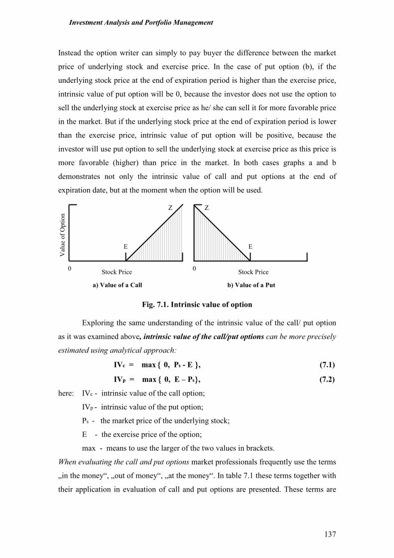
Investment Analysis and Portfolio Management
137
Instead the option writer can simply to pay buyer the difference between the market
price of underlying stock and exercise price. In the case of put option (b), if the
underlying stock price at the end of expiration period is higher than the exercise price,
intrinsic value of put option will be 0, because the investor does not use the option to
sell the underlying stock at exercise price as he/ she can sell it for more favorable price
in the market. But if the underlying stock price at the end of expiration period is lower
than the exercise price, intrinsic value of put option will be positive, because the
investor will use put option to sell the underlying stock at exercise price as this price is
more favorable (higher) than price in the market. In both cases graphs a and b
demonstrates not only the intrinsic value of call and put options at the end of
expiration date, but at the moment when the option will be used.
Fig. 7.1. Intrinsic value of option
Exploring the same understanding of the intrinsic value of the call/ put option
as it was examined above, intrinsic value of the call/put options can be more precisely
estimated using analytical approach:
IVc = max {{{{ 0, Ps - E }}}}, (7.1)
IVp = max {{{{ 0, E – Ps}}}}, (7.2)
here: IVc - intrinsic value of the call option;
IVp - intrinsic value of the put option;
Ps - the market price of the underlying stock;
E - the exercise price of the option;
max - means to use the larger of the two values in brackets.
When evaluating the call and put options market professionals frequently use the terms
„in the money“, „out of money“, „at the money“. In table 7.1 these terms together with
their application in evaluation of call and put options are presented. These terms are
Z
E
Val
ue
of
Op
tio
n
Stock Price 0
Z
E
0 Stock Price
a) Value of a Call b) Value of a Put
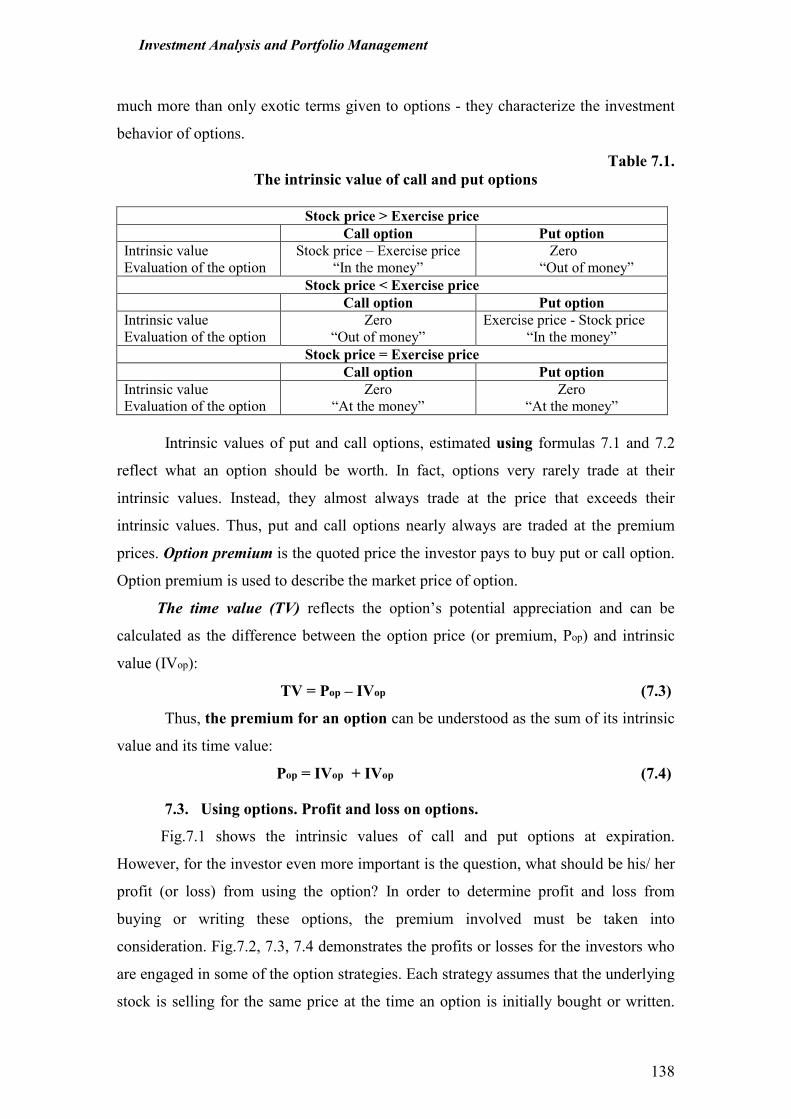
Investment Analysis and Portfolio Management
138
much more than only exotic terms given to options - they characterize the investment
behavior of options.
Table 7.1. The intrinsic value of call and put options
Stock price > Exercise price
Call option Put option Intrinsic value
Evaluation of the option
Stock price – Exercise price
“In the money”
Zero
“Out of money”
Stock price < Exercise price
Call option Put option Intrinsic value
Evaluation of the option
Zero
“Out of money”
Exercise price - Stock price
“In the money”
Stock price = Exercise price
Call option Put option Intrinsic value
Evaluation of the option
Zero
“At the money”
Zero
“At the money”
Intrinsic values of put and call options, estimated using formulas 7.1 and 7.2
reflect what an option should be worth. In fact, options very rarely trade at their
intrinsic values. Instead, they almost always trade at the price that exceeds their
intrinsic values. Thus, put and call options nearly always are traded at the premium
prices. Option premium is the quoted price the investor pays to buy put or call option.
Option premium is used to describe the market price of option.
The time value (TV) reflects the option’s potential appreciation and can be
calculated as the difference between the option price (or premium, Pop) and intrinsic
value (IVop):
TV = Pop – IVop (7.3)
Thus, the premium for an option can be understood as the sum of its intrinsic
value and its time value:
Pop = IVop + IVop (7.4)
7.3. Using options. Profit and loss on options.
Fig.7.1 shows the intrinsic values of call and put options at expiration.
However, for the investor even more important is the question, what should be his/ her
profit (or loss) from using the option? In order to determine profit and loss from
buying or writing these options, the premium involved must be taken into
consideration. Fig.7.2, 7.3, 7.4 demonstrates the profits or losses for the investors who
are engaged in some of the option strategies. Each strategy assumes that the underlying
stock is selling for the same price at the time an option is initially bought or written.
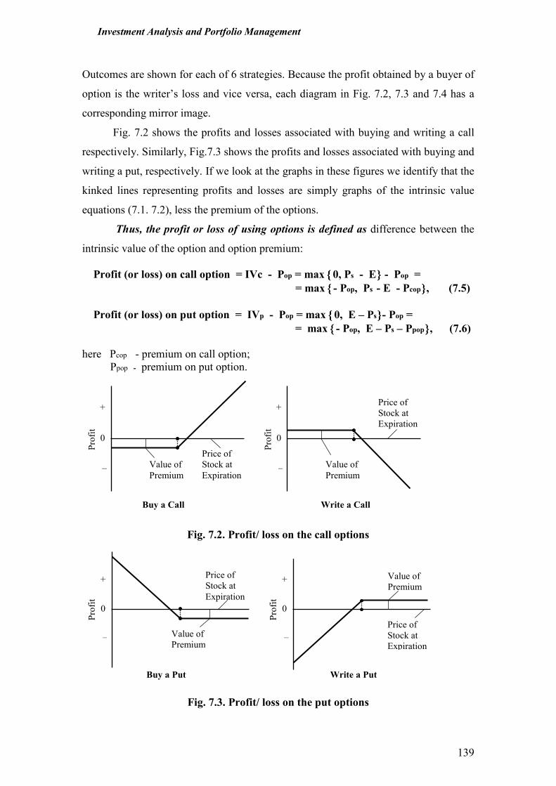
Investment Analysis and Portfolio Management
139
Outcomes are shown for each of 6 strategies. Because the profit obtained by a buyer of
option is the writer’s loss and vice versa, each diagram in Fig. 7.2, 7.3 and 7.4 has a
corresponding mirror image.
Fig. 7.2 shows the profits and losses associated with buying and writing a call
respectively. Similarly, Fig.7.3 shows the profits and losses associated with buying and
writing a put, respectively. If we look at the graphs in these figures we identify that the
kinked lines representing profits and losses are simply graphs of the intrinsic value
equations (7.1. 7.2), less the premium of the options.
Thus, the profit or loss of using options is defined as difference between the
intrinsic value of the option and option premium:
Profit (or loss) on call option = IVc - Pop = max {{{{0, Ps - E}}}} - Pop = = max {{{{- Pop, Ps - E - Pcop}}}}, (7.5)
Profit (or loss) on put option = IVp - Pop = max {{{{0, E – Ps}}}}- Pop = = max {{{{- Pop, E – Ps – Ppop}}}}, (7.6)
here Pcop - premium on call option;
Ppop - premium on put option.
Fig. 7.2. Profit/ loss on the call options
Fig. 7.3. Profit/ loss on the put options
+
Pro
fit
Value of
Premium
0
Buy a Call Write a Call
–
Price of
Stock at
Expiration
+
Pro
fit
Value of
Premium
0
–
Price of
Stock at
Expiration
Price of
Stock at
Expiration
+
Pro
fit
Value of
Premium
0
Buy a Put Write a Put
–
+
Pro
fit
Value of
Premium
0
–
Price of
Stock at
Expiration
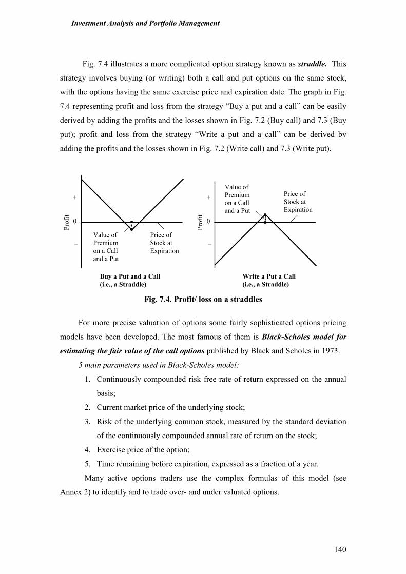
Investment Analysis and Portfolio Management
140
Fig. 7.4 illustrates a more complicated option strategy known as straddle. This
strategy involves buying (or writing) both a call and put options on the same stock,
with the options having the same exercise price and expiration date. The graph in Fig.
7.4 representing profit and loss from the strategy “Buy a put and a call” can be easily
derived by adding the profits and the losses shown in Fig. 7.2 (Buy call) and 7.3 (Buy
put); profit and loss from the strategy “Write a put and a call” can be derived by
adding the profits and the losses shown in Fig. 7.2 (Write call) and 7.3 (Write put).
Fig. 7.4. Profit/ loss on a straddles
For more precise valuation of options some fairly sophisticated options pricing
models have been developed. The most famous of them is Black-Scholes model for
estimating the fair value of the call options published by Black and Scholes in 1973.
5 main parameters used in Black-Scholes model:
1. Continuously compounded risk free rate of return expressed on the annual
basis;
2. Current market price of the underlying stock;
3. Risk of the underlying common stock, measured by the standard deviation
of the continuously compounded annual rate of return on the stock;
4. Exercise price of the option;
5. Time remaining before expiration, expressed as a fraction of a year.
Many active options traders use the complex formulas of this model (see
Annex 2) to identify and to trade over- and under valuated options.
Value of
Premium
on a Call
and a Put
+
Pro
fit
Value of
Premium
on a Call
and a Put
0
Buy a Put and a Call (i.e., a Straddle)
Write a Put a Call (i.e., a Straddle)
–
Price of
Stock at
Expiration
+ P
rofi
t
0
–
Price of
Stock at
Expiration
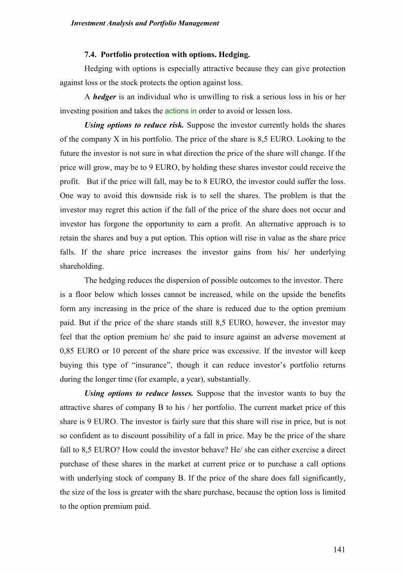
Investment Analysis and Portfolio Management
141
7.4. Portfolio protection with options. Hedging.
Hedging with options is especially attractive because they can give protection
against loss or the stock protects the option against loss.
A hedger is an individual who is unwilling to risk a serious loss in his or her
investing position and takes the actions in order to avoid or lessen loss.
Using options to reduce risk. Suppose the investor currently holds the shares
of the company X in his portfolio. The price of the share is 8,5 EURO. Looking to the
future the investor is not sure in what direction the price of the share will change. If the
price will grow, may be to 9 EURO, by holding these shares investor could receive the
profit. But if the price will fall, may be to 8 EURO, the investor could suffer the loss.
One way to avoid this downside risk is to sell the shares. The problem is that the
investor may regret this action if the fall of the price of the share does not occur and
investor has forgone the opportunity to earn a profit. An alternative approach is to
retain the shares and buy a put option. This option will rise in value as the share price
falls. If the share price increases the investor gains from his/ her underlying
shareholding.
The hedging reduces the dispersion of possible outcomes to the investor. There
is a floor below which losses cannot be increased, while on the upside the benefits
form any increasing in the price of the share is reduced due to the option premium
paid. But if the price of the share stands still 8,5 EURO, however, the investor may
feel that the option premium he/ she paid to insure against an adverse movement at
0,85 EURO or 10 percent of the share price was excessive. If the investor will keep
buying this type of “insurance”, though it can reduce investor’s portfolio returns
during the longer time (for example, a year), substantially.
Using options to reduce losses. Suppose that the investor wants to buy the
attractive shares of company B to his / her portfolio. The current market price of this
share is 9 EURO. The investor is fairly sure that this share will rise in price, but is not
so confident as to discount possibility of a fall in price. May be the price of the share
fall to 8,5 EURO? How could the investor behave? He/ she can either exercise a direct
purchase of these shares in the market at current price or to purchase a call options
with underlying stock of company B. If the price of the share does fall significantly,
the size of the loss is greater with the share purchase, because the option loss is limited
to the option premium paid.
Investment Analysis and Portfolio Management
142
Hedging portfolios of shares using index options. Large investors usually
manage varied portfolios of shares so, rather than hedging individual shareholdings
with options they may hedge their portfolios through the options on the entire index of
shares
Index option is based on stock index instead of an underlying stock. When
index option is exercised, settlement is made by cash payment, not delivery of shares.
The most often index options are settled on the bases of such indexes as
Standard&Poor’s 500 (USA); FTSE 100 (UK); DAX (Germany), CAC (France), etc.
Suppose, the investor manage a well diversified portfolio of shares and
currently is concerned that the market may fall over the next 3 months. One of possible
investment strategies for the investor is to buy the put option on the stock index. If the
market does fall, losses on the portfolio will be offset by gains on the value of the
index put option. If the portfolio is unhedged, the investor suffers from the market fall
substantially. But it is important to remember about the expenses of the insurance of
portfolio: when the options premiums are high (during periods of market volatility
caused by economic crises), hedging of the portfolio of stocks with index options over
longer period could be expensive.
Using hedging strategies very important characteristic is the hedge ratio of the
portfolio. Hedge ratio is a number of stocks to buy or sell with options such that the
future portfolio value is risk-free. The hedged portfolio consists of m purchased shares
and n options written (issued) on these shares.
Hedge ratio (HR) can be estimated using formula:
HR = m / n, (7.5)
here: m - number of shares in the portfolio;
n - a number of options written on the shares in the portfolio.
Riskless (perfect) hedge is when for m and n are chosen such a values which
allow in each moment given to compensate the decrease in prices of the stocks by
increase in value of options. This meaning of hedge ratio is called as a perfect hedge
ratio. But perfect hedge ratio could be achieved only under following assumptions:
• There are no transaction costs in the market;
• There are no taxes;
• The numbers of all traded securities is unlimited (including fractional
numbers);
Investment Analysis and Portfolio Management
143
• All the securities are available for trading permanently (24 hours) and at
any moment.
It is obvious that today even in the high developed markets these assumptions
can not be realized. Thus any hedged portfolio and its hedge ratio reflects only the
particular level of the “insurance” of the investor against the market risk.
Summary
1. Option is a type of contract between 2 persons where one person grants the other
person the right to buy or to sell a specific asset at a specific price within a specific
time period. The most often options are used in the trading of securities.
2. Two main types of option contracts: call option and put option. Call option gives
the buyer the right to buy (to call away) a specific number of shares of a specific
company from the option writer at a specific purchase price at any time up to
including a specific date. Put option gives the buyer the right to sell (to put away) a
specific number of shares of a specific company to the option writer at a specific
selling price at any time up to including a specific date.
3. The most important characteristics of option contract are exercise price (or strike
price) and expiration date. Exercise price is the purchase or selling price for the
underlying shares. Expiration date defines the time than the option contract
expires.
4. Regarding the condition when the option contract can be exercised two types of
call/ put options exist. European options can be exercised only on their expiration
dates. American options can be exercised any time during their life (defined by the
option contract).
5. The major advantages of investing in options are the possibility of hedging; an
investor can lose only a set amount of money (the purchase price of option);
options can be profitably when the price of the underlying security goes up or
down.
6. The major disadvantages of investing in options: the holder enjoys never interest
or dividend income nor any other ownership benefit; an investor has a limited time
frame in which to capture desired price behavior; this investment vehicle is a bit
complicated and many of its trading strategies are to complex for the non-
professional investor.
Investment Analysis and Portfolio Management
144
7. The value of put or call options is closely related with the market value/ price of
the security that underlies the option.
8. Intrinsic value for call option will be 0, if the underlying stock price at the end of
expiration period is less than the exercise price, intrinsic value of call option will
be positive, if the underlying stock price at the end of expiration period is higher
than the exercise price, because the investor will use call option to buy the
underlying stock at exercise price as this price is more favorable (lower) than price
in the market.
9. Intrinsic value for put option will be 0, if the underlying stock price at the end of
expiration period is higher than the exercise price, intrinsic value of put option will
be positive, if the underlying stock price at the end of expiration period is lower
than the exercise price, because the investor will use put option to sell the
underlying stock at exercise price as this price is more favorable (higher) than price
in the market.
10. „In the money“is a situation in which strike price of the option is below the market
price of underlying stock for a call, or the strike price is above the market price of
the underlying stock for a put.
11. „Out of money“is a situation in which strike price of the option is above the market
price of underlying stock for a call, or the strike price is below the market price of
the underlying stock for a put.
12. „At the money“is used to denote an option (put or call) whose strike price is at or
near the price of underlying stock.
13. Option premium is the quoted price the investor pays to buy put or call option.
Option premium is used to describe the market price of option.
14. The time value reflects the option’s potential appreciation and can be calculated as
the difference between the option price (premium) and intrinsic value.
15. The profit or loss of using options is defined as difference between the intrinsic
value of the option and option premium.
16. Black-Scholes model is developed for estimating the fair value of the call options.
5 main parameters used in Black-Scholes model are: (1) continuously compounded
risk free rate of return expressed on the annual basis; (2) current market price of the
underlying stock; (3) risk of the underlying common stock, measured by the
standard deviation of the continuously compounded annual rate of return on the
Investment Analysis and Portfolio Management
145
stock; (4) exercise price of the option; (5) time remaining before expiration,
expressed as a fraction of a year.
17. Option strategy known as straddle involves buying (or writing) both a call and put
options on the same stock, with the options having the same exercise price and
expiration date.
18. Hedging with options is especially attractive because they can give protection
against loss or the stock protects the option against loss. Hedging reduces the
dispersion of possible outcomes to the investor. There is a floor below which losses
cannot be increased, while the size of the loss would be limited to the option
premium paid.
19. Index option is based on stock index instead of an underlying stock. When index
option is exercised, settlement is made by cash payment, not delivery of shares.
20. Using hedging strategies very important characteristic is the hedge ratio of the
portfolio. Hedge ratio is a number of stocks to buy or sell with options such that
the future portfolio value is risk-free.
21. Riskless (perfect) hedge is such a hedge which allows in each moment given to
compensate the decrease in prices of the stocks by increase in value of options.
Key-terms
• American options
• „At the money“
• Black-Scholes model
• Call option
• European options
• Exercise price (strike price)
• Expiration date
• „In the money“
• Intrinsic value of option
• Hedger
• Hedging
• Hedge ratio
• Option
• Option buyer
• Option premium
• Option writer
• „Out of money“
• Riskless (perfect) hedge
• Perfect hedge ratio
• Put option
• Profit or loss on option
• Straddle
• Time value
• Underlying security
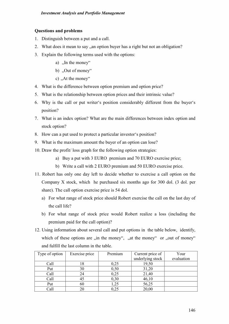
Investment Analysis and Portfolio Management
146
Questions and problems
1. Distinguish between a put and a call.
2. What does it mean to say „an option buyer has a right but not an obligation?
3. Explain the following terms used with the options:
a) „In the money“
b) „Out of money“
c) „At the money“
4. What is the difference between option premium and option price?
5. What is the relationship between option prices and their intrinsic value?
6. Why is the call or put writer‘s position considerably different from the buyer‘s
position?
7. What is an index option? What are the main differences between index option and
stock option?
8. How can a put used to protect a particular investor‘s position?
9. What is the maximum amount the buyer of an option can lose?
10. Draw the profit/ loss graph for the following option strategies:
a) Buy a put with 3 EURO premium and 70 EURO exercise price;
b) Write a call with 2 EURO premium and 50 EURO exercise price.
11. Robert has only one day left to decide whether to exercise a call option on the
Company X stock, which he purchased six months ago for 300 dol. (3 dol. per
share). The call option exercise price is 54 dol.
a) For what range of stock price should Robert exercise the call on the last day of
the call life?
b) For what range of stock price would Robert realize a loss (including the
premium paid for the call option)?
12. Using information about several call and put options in the table below, identify,
which of these options are „in the money“, „at the money“ or „out of money“
and fulfill the last column in the table.
Type of option Exercise price Premium Current price of
underlying stock
Your
evaluation
Call 18 0,25 19,50
Put 30 0,50 31,20
Call 24 0,25 21,40
Call 45 0,30 46,10
Put 60 1,25 56,25
Call 20 0,25 20,00
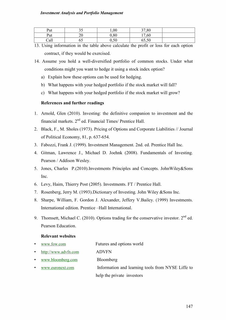
Investment Analysis and Portfolio Management
147
Put 35 1,00 37,80
Put 20 0,80 17,60
Call 65 0,50 65,50
13. Using information in the table above calculate the profit or loss for each option
contract, if they would be exercised.
14. Assume you hold a well-diversified portfolio of common stocks. Under what
conditions might you want to hedge it using a stock index option?
a) Explain how these options can be used for hedging.
b) What happens with your hedged portfolio if the stock market will fall?
c) What happens with your hedged portfolio if the stock market will grow?
References and further readings
1. Arnold, Glen (2010). Investing: the definitive companion to investment and the
financial markets. 2nd
ed. Financial Times/ Prentice Hall.
2. Black, F., M. Sholes (1973). Pricing of Options and Corporate Liabilities // Journal
of Political Economy, 81, p. 637-654.
3. Fabozzi, Frank J. (1999). Investment Management. 2nd. ed. Prentice Hall Inc.
4. Gitman, Lawrence J., Michael D. Joehnk (2008). Fundamentals of Investing.
Pearson / Addison Wesley.
5. Jones, Charles P.(2010).Investments Principles and Concepts. JohnWiley&Sons
Inc.
6. Levy, Haim, Thierry Post (2005). Investments. FT / Prentice Hall.
7. Rosenberg, Jerry M. (1993).Dictionary of Investing. John Wiley &Sons Inc.
8. Sharpe, William, F. Gordon J. Alexander, Jeffery V.Bailey. (1999) Investments.
International edition. Prentice –Hall International.
9. Thomsett, Michael C. (2010). Options trading for the conservative investor. 2nd
ed.
Pearson Education.
Relevant websites
• www.fow.com Futures and options world
• http://www.advfn.com ADVFN
• www.bloomberg.com Bloomberg
• www.euronext.com Information and learning tools from NYSE Liffe to
help the private investors
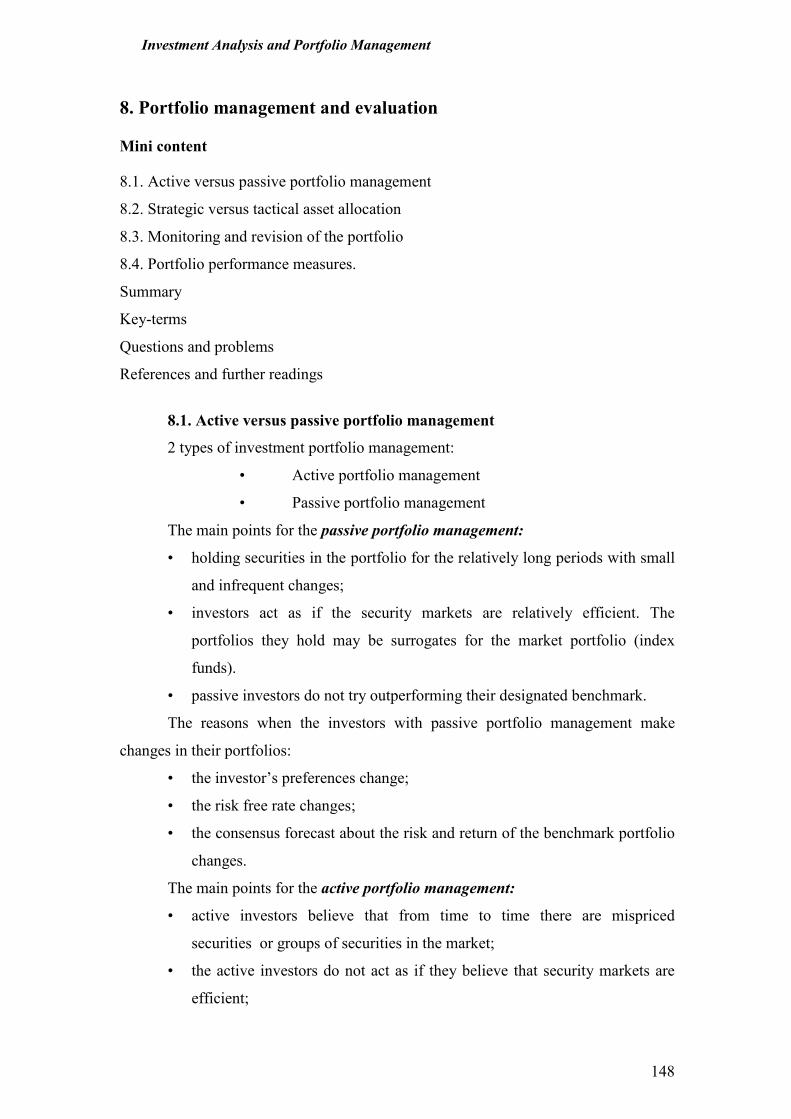
Investment Analysis and Portfolio Management
148
8. Portfolio management and evaluation
Mini content
8.1. Active versus passive portfolio management
8.2. Strategic versus tactical asset allocation
8.3. Monitoring and revision of the portfolio
8.4. Portfolio performance measures.
Summary
Key-terms
Questions and problems
References and further readings
8.1. Active versus passive portfolio management
2 types of investment portfolio management:
• Active portfolio management
• Passive portfolio management
The main points for the passive portfolio management:
• holding securities in the portfolio for the relatively long periods with small
and infrequent changes;
• investors act as if the security markets are relatively efficient. The
portfolios they hold may be surrogates for the market portfolio (index
funds).
• passive investors do not try outperforming their designated benchmark.
The reasons when the investors with passive portfolio management make
changes in their portfolios:
• the investor’s preferences change;
• the risk free rate changes;
• the consensus forecast about the risk and return of the benchmark portfolio
changes.
The main points for the active portfolio management:
• active investors believe that from time to time there are mispriced
securities or groups of securities in the market;
• the active investors do not act as if they believe that security markets are
efficient;
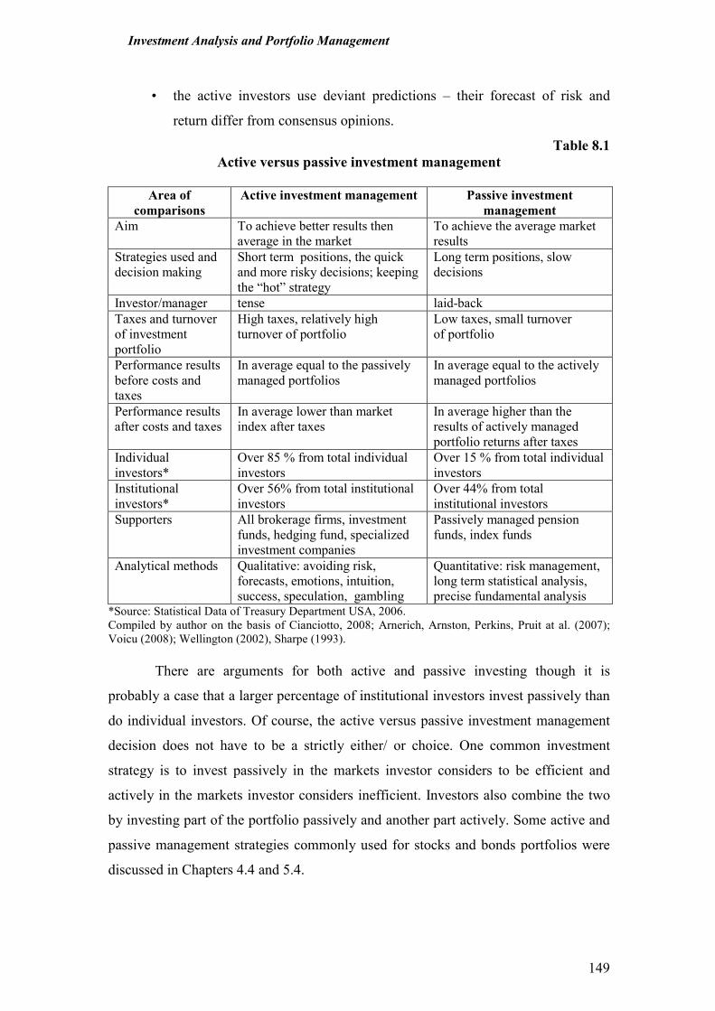
Investment Analysis and Portfolio Management
149
• the active investors use deviant predictions – their forecast of risk and
return differ from consensus opinions.
Table 8.1 Active versus passive investment management
Area of
comparisons Active investment management Passive investment
management Aim To achieve better results then
average in the market
To achieve the average market
results
Strategies used and
decision making
Short term positions, the quick
and more risky decisions; keeping
the “hot” strategy
Long term positions, slow
decisions
Investor/manager tense laid-back
Taxes and turnover
of investment
portfolio
High taxes, relatively high
turnover of portfolio
Low taxes, small turnover
of portfolio
Performance results
before costs and
taxes
In average equal to the passively
managed portfolios
In average equal to the actively
managed portfolios
Performance results
after costs and taxes
In average lower than market
index after taxes
In average higher than the
results of actively managed
portfolio returns after taxes
Individual
investors*
Over 85 % from total individual
investors
Over 15 % from total individual
investors
Institutional
investors*
Over 56% from total institutional
investors
Over 44% from total
institutional investors
Supporters All brokerage firms, investment
funds, hedging fund, specialized
investment companies
Passively managed pension
funds, index funds
Analytical methods Qualitative: avoiding risk,
forecasts, emotions, intuition,
success, speculation, gambling
Quantitative: risk management,
long term statistical analysis,
precise fundamental analysis *Source: Statistical Data of Treasury Department USA, 2006.
Compiled by author on the basis of Cianciotto, 2008; Arnerich, Arnston, Perkins, Pruit at al. (2007);
Voicu (2008); Wellington (2002), Sharpe (1993).
There are arguments for both active and passive investing though it is
probably a case that a larger percentage of institutional investors invest passively than
do individual investors. Of course, the active versus passive investment management
decision does not have to be a strictly either/ or choice. One common investment
strategy is to invest passively in the markets investor considers to be efficient and
actively in the markets investor considers inefficient. Investors also combine the two
by investing part of the portfolio passively and another part actively. Some active and
passive management strategies commonly used for stocks and bonds portfolios were
discussed in Chapters 4.4 and 5.4.
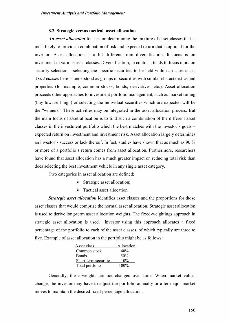
Investment Analysis and Portfolio Management
150
8.2. Strategic versus tactical asset allocation
An asset allocation focuses on determining the mixture of asset classes that is
most likely to provide a combination of risk and expected return that is optimal for the
investor. Asset allocation is a bit different from diversification. It focus is on
investment in various asset classes. Diversification, in contrast, tends to focus more on
security selection – selecting the specific securities to be held within an asset class.
Asset classes here is understood as groups of securities with similar characteristics and
properties (for example, common stocks; bonds; derivatives, etc.). Asset allocation
proceeds other approaches to investment portfolio management, such as market timing
(buy low, sell high) or selecting the individual securities which are expected will be
the “winners”. These activities may be integrated in the asset allocation process. But
the main focus of asset allocation is to find such a combination of the different asset
classes in the investment portfolio which the best matches with the investor’s goals –
expected return on investment and investment risk. Asset allocation largely determines
an investor’s success or lack thereof. In fact, studies have shown that as much as 90 %
or more of a portfolio’s return comes from asset allocation. Furthermore, researchers
have found that asset allocation has a much greater impact on reducing total risk than
does selecting the best investment vehicle in any single asset category.
Two categories in asset allocation are defined:
� Strategic asset allocation;
� Tactical asset allocation.
Strategic asset allocation identifies asset classes and the proportions for those
asset classes that would comprise the normal asset allocation. Strategic asset allocation
is used to derive long-term asset allocation weights. The fixed-weightings approach in
strategic asset allocation is used. Investor using this approach allocates a fixed
percentage of the portfolio to each of the asset classes, of which typically are three to
five. Example of asset allocation in the portfolio might be as follows:
Asset class Allocation Common stock 40%
Bonds 50%
Short-term securities 10%___
Total portfolio 100%
Generally, these weights are not changed over time. When market values
change, the investor may have to adjust the portfolio annually or after major market
moves to maintain the desired fixed-percentage allocation.
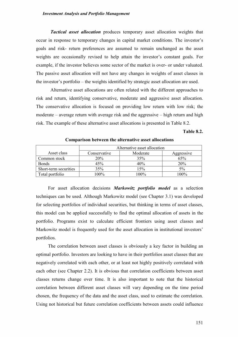
Investment Analysis and Portfolio Management
151
Tactical asset allocation produces temporary asset allocation weights that
occur in response to temporary changes in capital market conditions. The investor’s
goals and risk- return preferences are assumed to remain unchanged as the asset
weights are occasionally revised to help attain the investor’s constant goals. For
example, if the investor believes some sector of the market is over- or under valuated.
The passive asset allocation will not have any changes in weights of asset classes in
the investor’s portfolio – the weights identified by strategic asset allocation are used.
Alternative asset allocations are often related with the different approaches to
risk and return, identifying conservative, moderate and aggressive asset allocation.
The conservative allocation is focused on providing low return with low risk; the
moderate – average return with average risk and the aggressive – high return and high
risk. The example of these alternative asset allocations is presented in Table 8.2.
Table 8.2.
Comparison between the alternative asset allocations
Alternative asset allocation
Asset class Conservative Moderate Aggressive
Common stock 20% 35% 65%
Bonds 45% 40% 20%
Short-term securities 35% 15% 5%
Total portfolio 100% 100% 100%
For asset allocation decisions Markowitz portfolio model as a selection
techniques can be used. Although Markowitz model (see Chapter 3.1) was developed
for selecting portfolios of individual securities, but thinking in terms of asset classes,
this model can be applied successfully to find the optimal allocation of assets in the
portfolio. Programs exist to calculate efficient frontiers using asset classes and
Markowitz model is frequently used for the asset allocation in institutional investors’
portfolios.
The correlation between asset classes is obviously a key factor in building an
optimal portfolio. Investors are looking to have in their portfolios asset classes that are
negatively correlated with each other, or at least not highly positively correlated with
each other (see Chapter 2.2). It is obvious that correlation coefficients between asset
classes returns change over time. It is also important to note that the historical
correlation between different asset classes will vary depending on the time period
chosen, the frequency of the data and the asset class, used to estimate the correlation.
Using not historical but future correlation coefficients between assets could influence
Investment Analysis and Portfolio Management
152
the results remarkably, because the historical data may be different from the
expectations.
8.3. Monitoring and revision of the portfolio
Portfolio revision is the process of selling certain issues in portfolio and
purchasing new ones to replace them. The main reasons for the necessity of the
investment portfolio revision:
• As the economy evolves, certain industries and companies become either
less or more attractive as investments;
• The investor over the time may change his/her investment objectives and in
this way his/ her portfolio isn’t longer optimal;
• The constant need for diversification of the portfolio. Individual securities
in the portfolio often change in risk-return characteristics and their
diversification effect may be lessened.
Three areas to monitor when implementing investor’s portfolio monitoring:
1. Changes in market conditions;
2. Changes in investor’s circumstances;
3. Asset mix in the portfolio.
The need to monitor changes in the market is obvious. Investment decisions
are made in dynamic investment environment, where changes occur permanently. The
key macroeconomic indicators (such as GDP growth, inflation rate, interest rates,
others), as well as the new information about industries and companies should be
observed by investor on the regular basis, because these changes can influence the
returns and risk of the investments in the portfolio. Investor can monitor these changes
using various sources of information, especially specialized websites (most frequently
used are presented in relevant websites). It is important to identify he major changes in
the investment environment and to assess whether these changes should negatively
influence investor’s currently held portfolio. If it so investor must take an actions to
rebalance his/ her portfolio.
When monitoring the changes in the investor’s circumstances, following
aspects must be taken into account:
• Change in wealth
• Change in time horizon
• Change in liquidity requirements
Investment Analysis and Portfolio Management
153
• Change in tax circumstances
• Change in legal considerations
• Change in other circumstances and investor’s needs.
Any changes identified must be assessed very carefully before usually they
generally are related with the noticeable changes in investor’s portfolio.
Rebalancing a portfolio is the process of periodically adjusting it to maintain
certain original conditions. Rebalancing reduces the risks of losses – in general, a
rebalanced portfolio is less volatile than one that is not rebalanced. Several methods of
rebalancing portfolios are used:
� Constant proportion portfolio;
� Constant Beta portfolio;
� Indexing.
Constant proportion portfolio. A constant proportion portfolio is one in which
adjustments are made so as to maintain the relative weighting of the portfolio
components as their prices change. Investors should concentrate on keeping their
chosen asset allocation percentage (especially those following the requirements for
strategic asset allocation). There is no one correct formula for when to rebalance. One
rule may be to rebalance portfolio when asset allocations vary by 10% or more. But
many investors find it bizarre that constant proportion rebalancing requires the
purchase of securities that have performed poorly and the sale of those that have
performed the best. This is very difficult to do for the investor psychologically (see
Chapter 6). But the investor should always consider this method of rebalancing as one
choice, but not necessarily the best one.
Constant Beta portfolio. The base for the rebalancing portfolio using this
alternative is the target portfolio Beta. Over time the values of the portfolio
components and their Betas will change and this can cause the portfolio Beta to shift.
For example, if the target portfolio Beta is 1,10 and it had risen over the monitored
period of time to 1,25, the portfolio Beta could be brought back to the target (1,10) in
the following ways:
• Put additional money into the stock portfolio and hold cash. Diluting the
stocks in portfolio with the cash will reduce portfolio Beta, because cash has
Beta of 0. But in this case cash should be only a temporary component in the
portfolio rather than a long-term;
Investment Analysis and Portfolio Management
154
• Put additional money into the stock portfolio and buy stocks with a Beta
lower than the target Beta figure. But the investor may be is not able to
invest additional money and this way for rebalancing the portfolio can be
complicated.
• Sell high Beta stocks in portfolio and hold cash. As with the first
alternative, this way reduces the equity holdings in the investor’s portfolio
which may be not appropriate.
• Sell high Beta stocks and buy low Beta stocks. The stocks bought could
be new additions to the portfolio, or the investor could add to existing
positions.
Indexing. This alternatives for rebalancing the portfolio are more frequently
used by institutional investors (often mutual funds), because their portfolios tend to be
large and the strategy of matching a market index are best applicable for them.
Managing index based portfolio investor (or portfolio manager) eliminates concern
about outperforming the market, because by design, it seeks to behave just like the
market averages. Investor attempts to maintain some predetermined characteristics of
the portfolio, such as Beta of 1,0. The extent to which such a portfolio deviates from
its intended behaviors called tracking error.
Revising a portfolio is not without costs for an individual investor. These
costs can be direct costs – trading fees and commissions for the brokers who can
trade securities on the exchange. With the developing of alternative trading systems
(ATS) these costs can be decreased. It is important also, that the selling the securities
may have income tax implications which differ from country to country.
1.4.Portfolio performance measures
Portfolio performance evaluation involves determining periodically how the
portfolio performed in terms of not only the return earned, but also the risk
experienced by the investor. For portfolio evaluation appropriate measures of return
and risk as well as relevant standards (or “benchmarks”) are needed.
In general, the market value of a portfolio at a point of time is determined by
adding the markets value of all the securities held at that particular time. The market
value of the portfolio at the end of the period is calculated in the same way, only
using end-of-period prices of the securities held in the portfolio.
The return on the portfolio (rp):
Investment Analysis and Portfolio Management
155
rp = (Ve - Vb) / Vb, (8.1)
here: Ve - beginning value of the portfolio;
Vb - ending value of the portfolio.
The essential idea behind performance evaluation is to compare the returns
which were obtained on portfolio with the results that could be obtained if more
appropriate alternative portfolios had been chosen for the investment. Such
comparison portfolios are often referred to as benchmark portfolios. In selecting them
investor should be certain that they are relevant, feasible and known in advance. The
benchmark should reflect the objectives of the investor.
Portfolio Beta (see Chapter 3.3) can be used as an indication of the amount of
market risk that the portfolio had during the time interval. It can be compared directly
with the betas of other portfolios.
You cannot compare the ex post or the expected and the expected return of two
portfolios without adjusting for risk. To adjust the return for risk before comparison of
performance risk adjusted measures of performance can be used:
� Sharpe’s ratio;
� Treynor’s ratio;
� Jensen’s Alpha.
Sharpe’s ratio shows an excess a return over risk free rate, or risk premium, by
unit of total risk, measured by standard deviation:
Sharpe’s ratio = (řp– řf) / σp, (8.2)
here: řp - the average return for portfolio p during some period of time;
řf - the average risk-free rate of return during the period;
σp - standard deviation of returns for portfolio p during the period.
Treynor’s ratio shows an excess actual return over risk free rate, or risk
premium, by unit of systematic risk, measured by Beta:
Treynor’s ratio = (řp –řf) / βp, (8.3)
here: βp – Beta, measure of systematic risk for the portfolio p.
Jensen‘s Alpha shows excess actual return over required return and excess
of actual risk premium over required risk premium. This measure of the portfolio
manager’s performance is based on the CAPM (see Chapter 3.2).
Investment Analysis and Portfolio Management
156
Jensen’s Alpha = (řp– řf) – βp (řm –řf), (8.4)
here: řm - the average return on the market in period t;
(řm –řf) - the market risk premium during period t.
It is important to note, that if a portfolio is completely diversified, all of these
measures (Sharpe, Treynor’s ratios and Jensen’s alfa) will agree on the ranking of the
portfolios. The reason for this is that with the complete diversification total variance is
equal to systematic variance. When portfolios are not completely diversified, the
Treynor’s and Jensen’s measures can rank relatively undiversified portfolios much
higher than the Sharpe measure does. Since the Sharpe ratio uses total risk, both
systematic and unsystematic components are included.
Summary
1. The main points of passive portfolio management: holding securities in the
portfolio for the relatively long periods with small and infrequent changes;
investors act as if the security markets are relatively efficient; passive investors do
not try outperforming their designated benchmark.
2. The main points for the active portfolio management: active investors believe that
there are mispriced securities or groups of securities in the market; the active
investors do not act as if they believe that security markets are efficient; the active
investors use deviant predictions – their forecast of risk and return differ from
consensus opinions.
3. Strategic asset allocation identifies asset classes and the proportions for those asset
classes that would comprise the normal asset allocation. Strategic asset allocation
is used to derive long-term asset allocation weights. The fixed-weightings
approach in strategic asset allocation is used.
4. Tactical asset allocation produces temporary asset allocation weights that occur in
response to temporary changes in capital market conditions. The investor’s goals
and risk- return preferences are assumed to remain unchanged as the asset weights
are occasionally revised to help attain the investor’s constant goals.
5. For asset allocation decisions Markowitz portfolio model as a selection techniques
can be used. Thinking in terms of asset classes, this model can be applied
successfully to find the optimal allocation of assets in the portfolio. The
correlation between asset classes is a key factor in building such an optimal
portfolio. Investors are looking to have in their portfolios asset classes that are
Investment Analysis and Portfolio Management
157
negatively correlated with each other, or at least not highly positively correlated
with each other
6. Portfolio revision is the process of selling certain issues in portfolio and
purchasing new ones to replace them.
7. Three areas to monitor when implementing investor’s portfolio monitoring: (1)
Changes in market conditions; (2) Changes in investor’s circumstances; (3) Asset
mix in the portfolio.
8. When monitoring the changes in the investor’s circumstances, following aspects
must be taken into account: change in wealth; change in time horizon; change in
liquidity requirements; change in tax circumstances; change in legal
considerations; change in other circumstances and investor’s needs.
9. Rebalancing a portfolio is the process of periodically adjusting it to maintain
certain original conditions. Rebalancing reduces the risks of losses – in general, a
rebalanced portfolio is less volatile than one that is not rebalanced.
10. A constant proportion portfolio is one of the portfolio rebalancing methods in
which adjustments are made so as to maintain the relative weighting of the
portfolio components as their prices change. Investors should concentrate on
keeping their chosen asset allocation percentage (especially those following the
requirements for strategic asset allocation).
11. The bases for the rebalancing portfolio using constant Beta portfolio alternative is
the target portfolio Beta. Over time the values of the portfolio components and
their Betas might change. This can cause the portfolio Beta to shift and then the
portfolio Beta should be brought back to the target.
12. Using indexing method for rebalancing the portfolio the investors match a market
index best applicable for them. Managing index based portfolio investor (or
portfolio manager) eliminates concern about outperforming the market, because by
design, it seeks to behave just like the market averages.
13. Portfolio performance evaluation involves determining periodically how the
portfolio performed in terms of not only the return earned, but also the risk
experienced by the investor. For portfolio evaluation appropriate measures of
return and risk as well as relevant standards (or “benchmarks”) are needed. In
selecting benchmark portfolios investor should be certain that they are relevant,
Investment Analysis and Portfolio Management
158
feasible and known in advance. The benchmark should reflect the objectives of the
investor.
14. To adjust the return for risk before comparison of performance risk adjusted
measures of performance can be used. Sharpe’s ratio shows an excess a return over
risk free rate, or risk premium, by unit of total risk, measured by standard
deviation. Treynor’s ratio shows an excess actual return over risk free rate, or risk
premium, by unit of systematic risk, measured by Beta. Jensen‘s Alpha shows
excess actual return over required return and excess of actual risk premium over
required risk premium. This measure of the portfolio manager’s performance is
based on the CAPM.
Key-terms
• Asset classes
• Asset allocation
• Sharpe’s ratio
• Treynor’s ratio
• Jensen’s Alpha
• Benchmark portfolios
• Tracking error
• Constant proportion portfolio method
• Constant Beta portfolio method
• Indexing method
• Rebalancing a portfolio
• Portfolio monitoring
• Portfolio revision
• Strategic asset allocation
• Tactical asset allocation.
• Active portfolio management
• Passive portfolio management
Questions and problems
1. Give the arguments for active portfolio management.
2. What are the reasons which cause investors managing their portfolios passively to
make changes their portfolios?
3. What are the major differences between active and passive portfolio management?
4. Explain the role of revision in the process of managing a portfolio.
5. Distinguish strategic and tactical asset allocation.
6. What role does current market information play in managing investment portfolio?
7. Why is the asset allocation decision the most important decision made by
investors?
8. What is the point of investment portfolio rebalancing?
Investment Analysis and Portfolio Management
159
9. What changes in investor’s circumstances cause the rebalancing of the investment
portfolio? Explain why.
10. Why is portfolio revision not free of cost?
11. Why benchmark portfolios are important in investment portfolio management?
12. Briefly describe each of the portfolio performance measures and explain how they
are used:
a) Sharpe’s ratio;
b) Treynor’s ratio;
c) Jensen’s Alpha.
13. Assume that you plan to construct a portfolio aimed at achieving your stated
objectives. The portfolio can be constructed by allocating your money to the
following asset classes: common stock, bonds, and short-term securities.
a) Identify state and comment your investment objectives.
b) Determine an asset allocation to these three classes of assets considering
your stated investment objectives. Explain your decision.
c) What reasons could cause you to make changes in your asset allocations?
14. An investor’s portfolio consists of 50000 EURO in stocks and 5000 EURO in
cash. the Beta of the portfolio is 1,10. How the investor could reduce Beta of the
portfolio to 0,95? Show and explain.
15. Select four stocks which were actively traded in the local stock exchange last
calendar year, find the information about their prices at the beginning and at the
end of the year, amount of dividends paid on each stock for this year and stock
Beta at the end of the year. Also find a risk-free rate of return and the market
return for the given year. Assume that these four stocks were put to the portfolio
in equal proportions (25% in each stock). Assume that the standard deviation for
this portfolio is 16, 75% and that standard deviation for the market portfolio is
13, 50%.
a) Find the portfolio return for the given year (see chapter 3.1.2, formula 3.1).
b) Calculate Sharpe’s, Treynor’s ratios and Jensen’s Alpha.
c) Compare and comment the results of measuring portfolio performance with
different measures.
Investment Analysis and Portfolio Management
160
References and further readings
1. Arnerich, T., at al. (2007) Active .versus passive investment management: putting
the debate into perspective // Journal of Financial Research, spring.
2. Arnold, Glen (2010). Investing: the definitive companion to investment and the
financial markets. 2nd
ed. Financial Times/ Prentice Hall.
3. Bogle, J.C. (2001) Three challenges of investing: active management, market
efficiency, and selecting managers // Journal of Financial Research, spring.
4. Brands, S., Brown, S. J., Gallagher, D.R. (2005) Portfolio concentration and
investment performance // Journal of Banking and Finance, spring.
5. Brands, S., Gallagher, D.R., Looi, A. (2003) Active investment manager portfolios
and preferences for stock characteristics: Australian evidence // Securities Industry
Research Centre of Asia-Pacific.
6. Cianciotto, Ph. (2008) Improving your investment returns – passive or active
investing // AAL financial planning association.
7. Fabozzi, Frank J. (1999). Investment Management. 2nd. ed. Prentice Hall Inc.
8. Francis, Jack C., Roger Ibbotson (2002). Investments: A Global Perspective.
Prentice Hall Inc.
9. Gallagher, D.R. (2003) Investment manager characteristics, strategy, top
management changes and fund performance // The Journal of Banking and
Finance, spring.
10. Gallagher, D.R., Nadarajah, P. (2004) Top management turnover: an analysis of
active Australian investment managers // The Journal of Banking and Finance,
winter.
11. Gitman, Lawrence J., Michael D. Joehnk (2008). Fundamentals of Investing.
Pearson / Addison Wesley.
12. Gold, M. (2004) Investing in pseudo-science: the `active versus passive` debate //
The Journal of Financial Research, spring.
13. Jones, Charles P. (2010). Investments Principles and Concepts. John Wiley &
Sons, Inc.
14. LeBarron, Dean, Romeesh Vaitilingam. (1999). Ultimate Investor. Capstone.
15. Nakamura, L. (2005) A comparison of active and passive investment strategies //
The Journal of Financial Research, spring.
Investment Analysis and Portfolio Management
161
16. Rice, M., Strotman, G. (2007) The next chapter in the active vs. passive
management debate // LLC research and analysis, spring.
17. Rosenberg, Jerry M. (1993).Dictionary of Investing. John Wiley &Sons Inc.
18. Sharpe, William. The Arithmetic of Active Management. // Financial Analysis
Journal, 1991.
19. Strong, Robert A. (1993). Portfolio Construction, Management and Protection.
West Publishing Company.
20. Voicu, A., (2008) Passive vs. active investment management strategies // The
financial planning association, spring.
21. Wellington, J.W. (2002) Active vs. passive management // The Journal of
Financial Research, spring.
Relevant websites
• www.morningstar.co.uk Morningstar UK
• www.funds.ft.com/funds Financial Times Fund Services
• www.funds-sp.com Standard &Poor‘s Fund Service
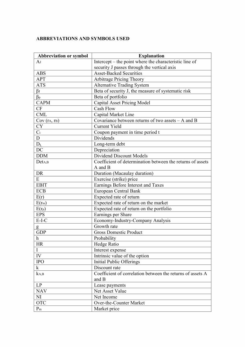
ABBREVIATIONS AND SYMBOLS USED
Abbreviation or symbol Explanation AJ Intercept – the point where the characteristic line of
security J passes through the vertical axis
ABS Asset-Backed Securities
APT Arbitrage Pricing Theory
ATS Alternative Trading System
βJ Beta of security J, the measure of systematic risk
βp Beta of portfolio
CAPM Capital Asset Pricing Model
CF Cash Flow
CML Capital Market Line
Cov (rA, rB) Covariance between returns of two assets – A and B
CY Current Yield
Ct Coupon payment in time period t
D Dividends
DL Long-term debt
DC Depreciation
DDM Dividend Discount Models
DetA,B Coefficient of determination between the returns of assets
A and B
DR Duration (Macaulay duration)
E Exercise (strike) price
EBIT Earnings Before Interest and Taxes
ECB European Central Bank
E(r) Expected rate of return
E(rm) Expected rate of return on the market
E(rp) Expected rate of return on the portfolio
EPS Earnings per Share
E-I-C Economy-Industry-Company Analysis
g Growth rate
GDP Gross Domestic Product
h Probability
HR Hedge Ratio
I Interest expense
IV Intrinsic value of the option
IPO Initial Public Offerings
k Discount rate
kA,B Coefficient of correlation between the returns of assets A
and B
LP Lease payments
NAV Net Asset Value
NI Net Income
OTC Over-the-Counter Market
Pm Market price
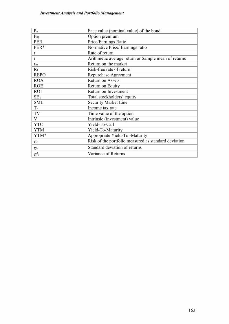
Investment Analysis and Portfolio Management
163
Pn Face value (nominal value) of the bond
Pop Option premium
PER Price/Earnings Ratio
PER* Normative Price/ Earnings ratio
r Rate of return
ŕ Arithmetic average return or Sample mean of returns
rm Return on the market
Rf Risk-free rate of return
REPO Repurchase Agreement
ROA Return on Assets
ROE Return on Equity
ROI Return on Investment
SET Total stockholders’ equity
SML Security Market Line
Tr Income tax rate
TV Time value of the option
V Intrinsic (investment) value
YTC Yield-To-Call
YTM Yield-To-Maturity
YTM* Appropriate Yield-To -Maturity
σp Risk of the portfolio measured as standard deviation
σr Standard deviation of returns
σ²r Variance of Returns
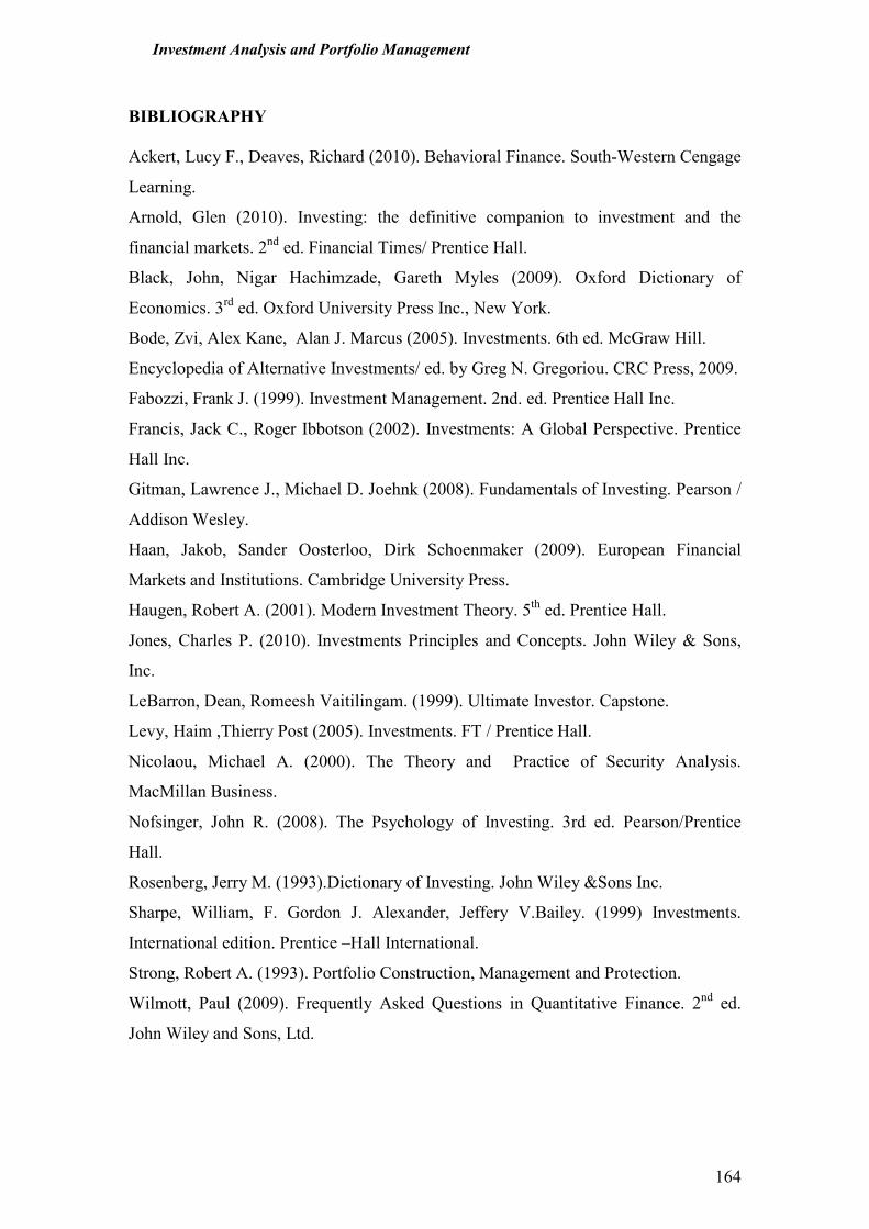
Investment Analysis and Portfolio Management
164
BIBLIOGRAPHY
Ackert, Lucy F., Deaves, Richard (2010). Behavioral Finance. South-Western Cengage
Learning.
Arnold, Glen (2010). Investing: the definitive companion to investment and the
financial markets. 2nd
ed. Financial Times/ Prentice Hall.
Black, John, Nigar Hachimzade, Gareth Myles (2009). Oxford Dictionary of
Economics. 3rd
ed. Oxford University Press Inc., New York.
Bode, Zvi, Alex Kane, Alan J. Marcus (2005). Investments. 6th ed. McGraw Hill.
Encyclopedia of Alternative Investments/ ed. by Greg N. Gregoriou. CRC Press, 2009.
Fabozzi, Frank J. (1999). Investment Management. 2nd. ed. Prentice Hall Inc.
Francis, Jack C., Roger Ibbotson (2002). Investments: A Global Perspective. Prentice
Hall Inc.
Gitman, Lawrence J., Michael D. Joehnk (2008). Fundamentals of Investing. Pearson /
Addison Wesley.
Haan, Jakob, Sander Oosterloo, Dirk Schoenmaker (2009). European Financial
Markets and Institutions. Cambridge University Press.
Haugen, Robert A. (2001). Modern Investment Theory. 5th
ed. Prentice Hall.
Jones, Charles P. (2010). Investments Principles and Concepts. John Wiley & Sons,
Inc.
LeBarron, Dean, Romeesh Vaitilingam. (1999). Ultimate Investor. Capstone.
Levy, Haim ,Thierry Post (2005). Investments. FT / Prentice Hall.
Nicolaou, Michael A. (2000). The Theory and Practice of Security Analysis.
MacMillan Business.
Nofsinger, John R. (2008). The Psychology of Investing. 3rd ed. Pearson/Prentice
Hall.
Rosenberg, Jerry M. (1993).Dictionary of Investing. John Wiley &Sons Inc.
Sharpe, William, F. Gordon J. Alexander, Jeffery V.Bailey. (1999) Investments.
International edition. Prentice –Hall International.
Strong, Robert A. (1993). Portfolio Construction, Management and Protection.
Wilmott, Paul (2009). Frequently Asked Questions in Quantitative Finance. 2nd
ed.
John Wiley and Sons, Ltd.
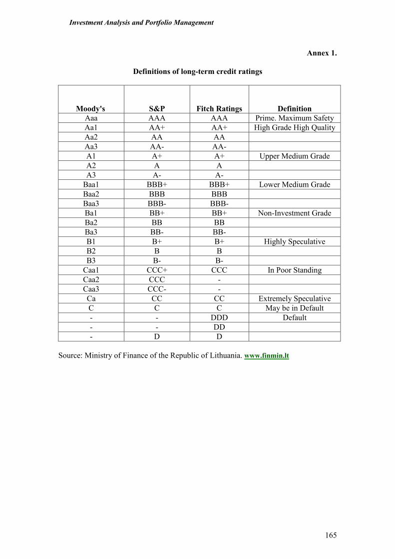
Investment Analysis and Portfolio Management
165
Annex 1.
Definitions of long-term credit ratings
Moody's
S&P
Fitch Ratings
Definition
Aaa AAA AAA Prime. Maximum Safety
Aa1 AA+ AA+ High Grade High Quality
Aa2 AA AA
Aa3 AA- AA-
A1 A+ A+ Upper Medium Grade
A2 A A
A3 A- A-
Baa1 BBB+ BBB+ Lower Medium Grade
Baa2 BBB BBB
Baa3 BBB- BBB-
Ba1 BB+ BB+ Non-Investment Grade
Ba2 BB BB
Ba3 BB- BB-
B1 B+ B+ Highly Speculative
B2 B B
B3 B- B-
Caa1 CCC+ CCC In Poor Standing
Caa2 CCC -
Caa3 CCC- -
Ca CC CC Extremely Speculative
C C C May be in Default
- - DDD Default
- - DD
- D D
Source: Ministry of Finance of the Republic of Lithuania. www.finmin.lt
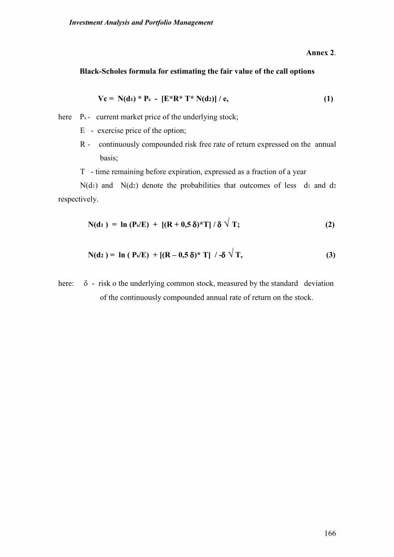
Investment Analysis and Portfolio Management
166
Annex 2.
Black-Scholes formula for estimating the fair value of the call options Vc = N(d1) * Ps - [E*R* T* N(d2)] / e, (1)
here Ps - current market price of the underlying stock;
E - exercise price of the option;
R - continuously compounded risk free rate of return expressed on the annual
basis;
T - time remaining before expiration, expressed as a fraction of a year
N(d1) and N(d2) denote the probabilities that outcomes of less d1 and d2
respectively.
N(d1 ) = ln (Ps/E) + [(R + 0,5 δδδδ)*T] / δδδδ √ T; (2)
N(d2 ) = ln ( Ps/E) + [(R – 0,5 δδδδ)* T] / -δδδδ √ T, (3) here: δ - risk o the underlying common stock, measured by the standard deviation
of the continuously compounded annual rate of return on the stock.


