Download - Introduction to Logistic Regression Modeling - minitab.com · Logistic Regression will estimate binary (Cox (1970)) and multinomial (Anderson (1972)) logistic models. Logistic Regression

Introduction to Logistic Regression Modeling

2

© 2019 Minitab, LLC. All Rights Reserved.

Minitab®, SPM®, SPM Salford Predictive Modeler®, Salford Predictive Modeler®, Random Forests®, CART®, TreeNet®, MARS®, RuleLearner®, and the Minitab logo are registered trademarks of Minitab, LLC. in the United States and other countries. Additional trademarks of Minitab, LLC. can be found at www.minitab.com. All other marks referenced remain the property of their respective owners.

www.minitab.com

Salford Predictive Modeler® Introduction to Logistic Regression Modeling

3

Introducing Logistic Regression Module

The Logistic Regression module is the SPM's tool for logistic regression analysis, and provides for model

building, model evaluation, prediction and scoring, and regression diagnostics. Logistic Regression is

designed to be easy to use for the novice and can produce the results most analysts need with just three

simple commands or menu options. Yet many advanced features are also included for sophisticated

research projects.

Logistic Regression will estimate binary (Cox (1970)) and multinomial (Anderson (1972)) logistic models.

Logistic Regression is designed for analyzing the determinants of a categorical dependent variable.

Typically, the dependent variable is binary and coded as 0 or 1; however, it may be multinomial and is

often coded as an integer ranging from 1 to K but could be, for instance, coded as a series of character

strings, e.g., "Republican", "Democrat", "Independent", and “Non Voter". Studies one can conduct with

Logistic Regression include bioassay, epidemiology of disease (cohort or case-control), clinical trials,

market research, transportation research (mode of travel), psychometric studies, and voter choice

analysis.

This manual contains a brief introduction to logistic regression and a full description of the commands and

features of the module. If you are unfamiliar with logistic regression, the textbook by Hosmer and

Lemeshow (1989) is an excellent place to begin; Breslow and Day (1980) provide an introduction in the

context of case-control studies, Train (1986) and Ben-Akiva and Lerman (1985) introduce the discrete

choice model for econometrics, Wrigley (1985) discusses the model for geographers, and Hoffman and

Duncan (1988) review discrete choice in a demographic-sociological context. Valuable surveys appear in

Amemiya (1981), McFadden (1984, 1982, 1976) and Maddala (1983)). This is just a small sampling from

a rather large literature; other specialty references are cited later in this chapter.

The best way to learn to use Logistic Regression is to read the QUICKSTART section which follows and

try the program out. Later you can selectively read the more detailed documentation or refer to the

appendices containing reference material on each command.


4

Logistic Regression QUICKSTART

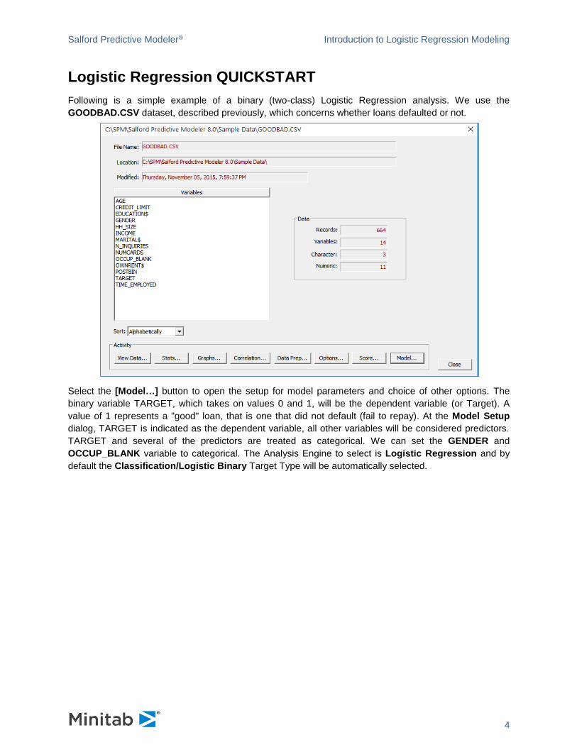
Following is a simple example of a binary (two-class) Logistic Regression analysis. We use the

GOODBAD.CSV dataset, described previously, which concerns whether loans defaulted or not.

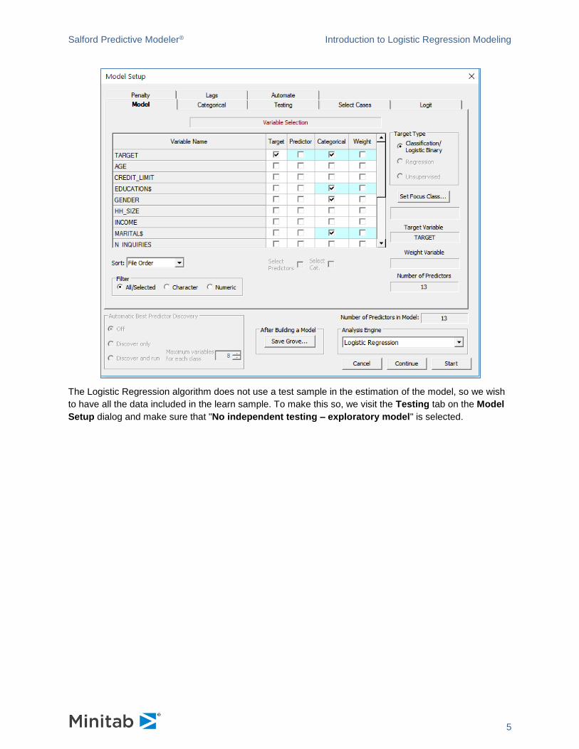
Select the [Model…] button to open the setup for model parameters and choice of other options. The

binary variable TARGET, which takes on values 0 and 1, will be the dependent variable (or Target). A

value of 1 represents a "good" loan, that is one that did not default (fail to repay). At the Model Setup

dialog, TARGET is indicated as the dependent variable, all other variables will be considered predictors.

TARGET and several of the predictors are treated as categorical. We can set the GENDER and

OCCUP_BLANK variable to categorical. The Analysis Engine to select is Logistic Regression and by

default the Classification/Logistic Binary Target Type will be automatically selected.


5

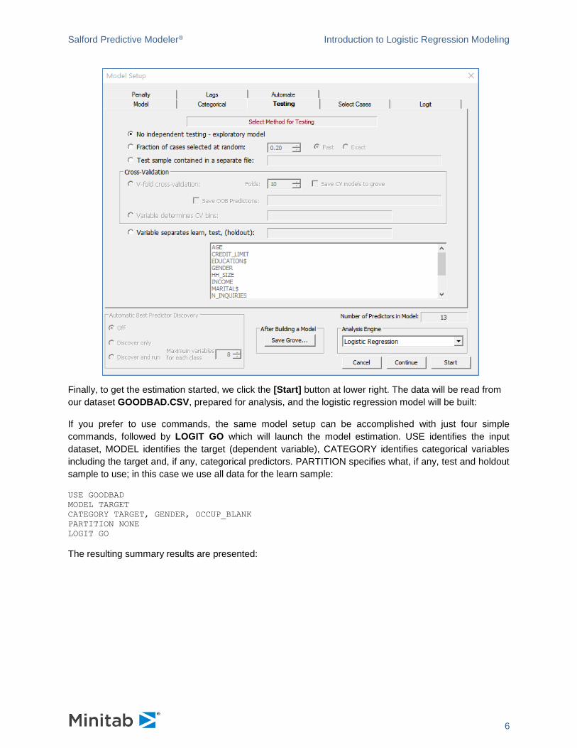
The Logistic Regression algorithm does not use a test sample in the estimation of the model, so we wish

to have all the data included in the learn sample. To make this so, we visit the Testing tab on the Model

Setup dialog and make sure that "No independent testing – exploratory model" is selected.


6

Finally, to get the estimation started, we click the [Start] button at lower right. The data will be read from

our dataset GOODBAD.CSV, prepared for analysis, and the logistic regression model will be built:

If you prefer to use commands, the same model setup can be accomplished with just four simple

commands, followed by LOGIT GO which will launch the model estimation. USE identifies the input

dataset, MODEL identifies the target (dependent variable), CATEGORY identifies categorical variables

including the target and, if any, categorical predictors. PARTITION specifies what, if any, test and holdout

sample to use; in this case we use all data for the learn sample:

USE GOODBAD

MODEL TARGET

CATEGORY TARGET, GENDER, OCCUP_BLANK

PARTITION NONE

LOGIT GO

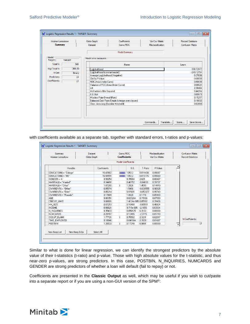
The resulting summary results are presented:


7

with coefficients available as a separate tab, together with standard errors, t-ratios and p-values:

Similar to what is done for linear regression, we can identify the strongest predictors by the absolute

value of their t-statistics (t-ratio) and p-value. Those with high absolute values for the t-statistic, and thus

near-zero p-values, are strong predictors. In this case, POSTBIN, N_INQUIRIES, NUMCARDS and

GENDER are strong predictors of whether a loan will default (fail to repay) or not.

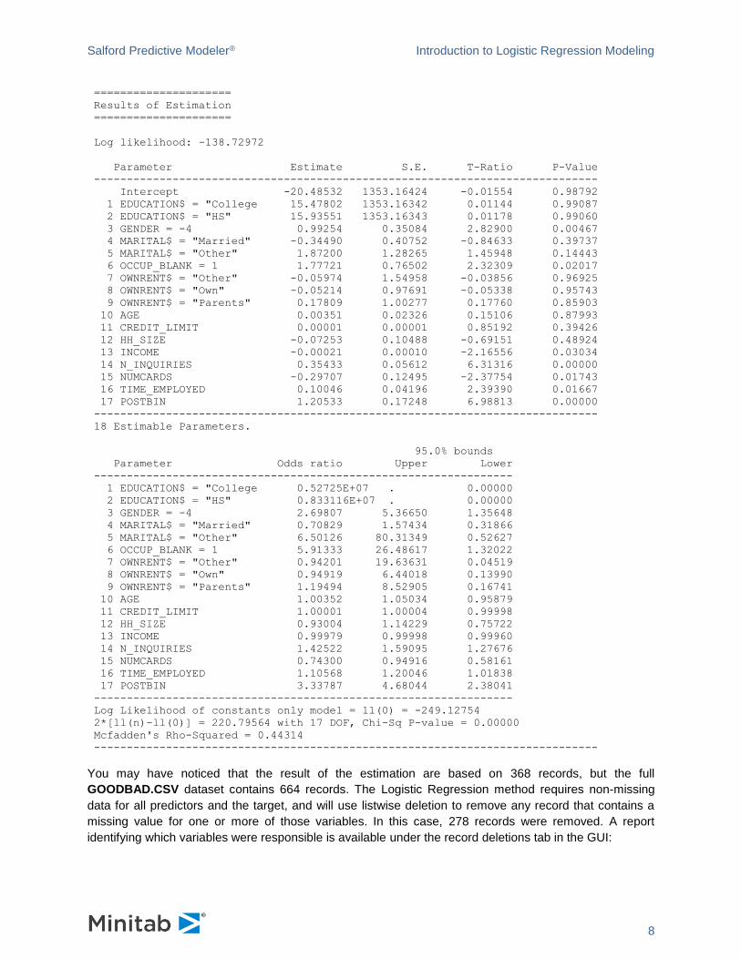
Coefficients are presented in the Classic Output as well, which may be useful if you wish to cut/paste

into a separate report or if you are using a non-GUI version of the SPM®:


8

=====================

Results of Estimation

=====================

Log likelihood: -138.72972

Parameter Estimate S.E. T-Ratio P-Value

-----------------------------------------------------------------------------

Intercept -20.48532 1353.16424 -0.01554 0.98792

1 EDUCATION$ = "College 15.47802 1353.16342 0.01144 0.99087

2 EDUCATION$ = "HS" 15.93551 1353.16343 0.01178 0.99060

3 GENDER = -4 0.99254 0.35084 2.82900 0.00467

4 MARITAL$ = "Married" -0.34490 0.40752 -0.84633 0.39737

5 MARITAL$ = "Other" 1.87200 1.28265 1.45948 0.14443

6 OCCUP_BLANK = 1 1.77721 0.76502 2.32309 0.02017

7 OWNRENT$ = "Other" -0.05974 1.54958 -0.03856 0.96925

8 OWNRENT$ = "Own" -0.05214 0.97691 -0.05338 0.95743

9 OWNRENT$ = "Parents" 0.17809 1.00277 0.17760 0.85903

10 AGE 0.00351 0.02326 0.15106 0.87993

11 CREDIT_LIMIT 0.00001 0.00001 0.85192 0.39426

12 HH_SIZE -0.07253 0.10488 -0.69151 0.48924

13 INCOME -0.00021 0.00010 -2.16556 0.03034

14 N_INQUIRIES 0.35433 0.05612 6.31316 0.00000

15 NUMCARDS -0.29707 0.12495 -2.37754 0.01743

16 TIME_EMPLOYED 0.10046 0.04196 2.39390 0.01667

17 POSTBIN 1.20533 0.17248 6.98813 0.00000

-----------------------------------------------------------------------------

18 Estimable Parameters.

95.0% bounds

Parameter Odds ratio Upper Lower

----------------------------------------------------------------

1 EDUCATION$ = "College 0.52725E+07 . 0.00000

2 EDUCATION$ = "HS" 0.833116E+07 . 0.00000

3 GENDER = -4 2.69807 5.36650 1.35648

4 MARITAL$ = "Married" 0.70829 1.57434 0.31866

5 MARITAL$ = "Other" 6.50126 80.31349 0.52627

6 OCCUP_BLANK = 1 5.91333 26.48617 1.32022

7 OWNRENT$ = "Other" 0.94201 19.63631 0.04519

8 OWNRENT$ = "Own" 0.94919 6.44018 0.13990

9 OWNRENT$ = "Parents" 1.19494 8.52905 0.16741

10 AGE 1.00352 1.05034 0.95879

11 CREDIT_LIMIT 1.00001 1.00004 0.99998

12 HH_SIZE 0.93004 1.14229 0.75722

13 INCOME 0.99979 0.99998 0.99960

14 N_INQUIRIES 1.42522 1.59095 1.27676

15 NUMCARDS 0.74300 0.94916 0.58161

16 TIME_EMPLOYED 1.10568 1.20046 1.01838

17 POSTBIN 3.33787 4.68044 2.38041

----------------------------------------------------------------

Log Likelihood of constants only model = ll(0) = -249.12754

2*[ll(n)-ll(0)] = 220.79564 with 17 DOF, Chi-Sq P-value = 0.00000

Mcfadden's Rho-Squared = 0.44314

-----------------------------------------------------------------------------

You may have noticed that the result of the estimation are based on 368 records, but the full

GOODBAD.CSV dataset contains 664 records. The Logistic Regression method requires non-missing

data for all predictors and the target, and will use listwise deletion to remove any record that contains a

missing value for one or more of those variables. In this case, 278 records were removed. A report

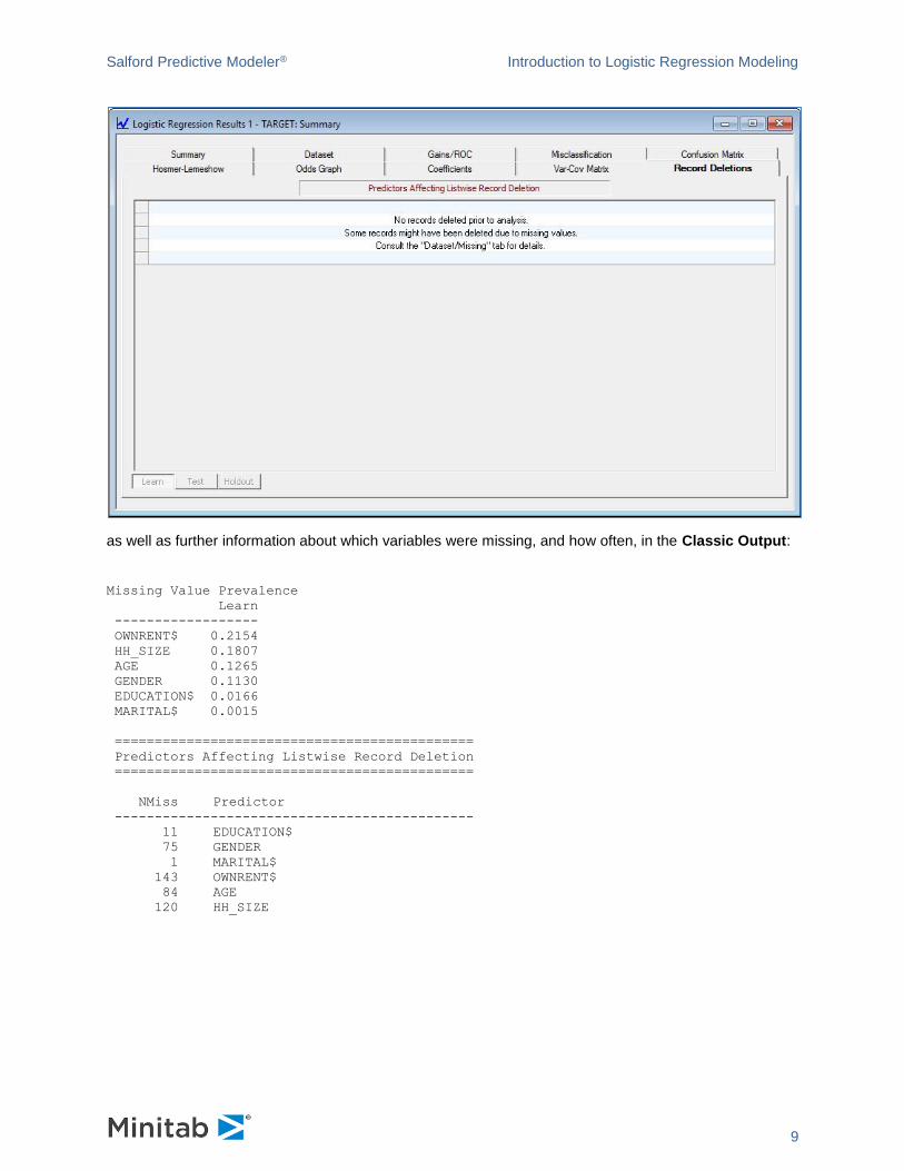
identifying which variables were responsible is available under the record deletions tab in the GUI:


9

as well as further information about which variables were missing, and how often, in the Classic Output:

Missing Value Prevalence

Learn

------------------

OWNRENT$ 0.2154

HH_SIZE 0.1807

AGE 0.1265

GENDER 0.1130

EDUCATION$ 0.0166

MARITAL$ 0.0015

=============================================

Predictors Affecting Listwise Record Deletion

=============================================

NMiss Predictor

---------------------------------------------

11 EDUCATION$

75 GENDER

1 MARITAL$

143 OWNRENT$

84 AGE

120 HH_SIZE


10

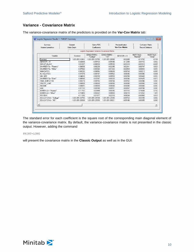
Variance - Covariance Matrix

The variance-covariance matrix of the predictors is provided on the Var-Cov Matrix tab:

The standard error for each coefficient is the square root of the corresponding main diagonal element of

the variance-covariance matrix. By default, the variance-covariance matrix is not presented in the classic

output. However, adding the command

PRINT=LONG

will present the covariance matrix in the Classic Output as well as in the GUI:


11

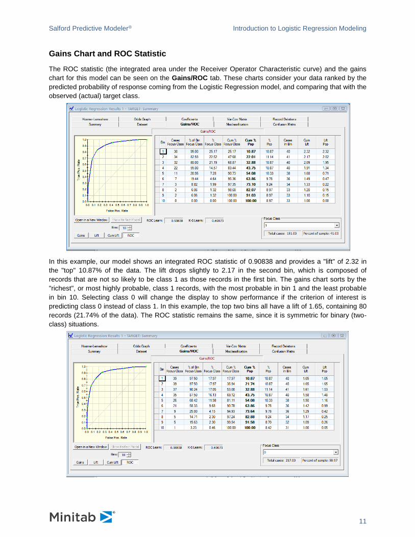
Gains Chart and ROC Statistic

The ROC statistic (the integrated area under the Receiver Operator Characteristic curve) and the gains

chart for this model can be seen on the Gains/ROC tab. These charts consider your data ranked by the

predicted probability of response coming from the Logistic Regression model, and comparing that with the

observed (actual) target class.

In this example, our model shows an integrated ROC statistic of 0.90838 and provides a "lift" of 2.32 in

the "top" 10.87% of the data. The lift drops slightly to 2.17 in the second bin, which is composed of

records that are not so likely to be class 1 as those records in the first bin. The gains chart sorts by the

"richest", or most highly probable, class 1 records, with the most probable in bin 1 and the least probable

in bin 10. Selecting class 0 will change the display to show performance if the criterion of interest is

predicting class 0 instead of class 1. In this example, the top two bins all have a lift of 1.65, containing 80

records (21.74% of the data). The ROC statistic remains the same, since it is symmetric for binary (two-

class) situations.


12

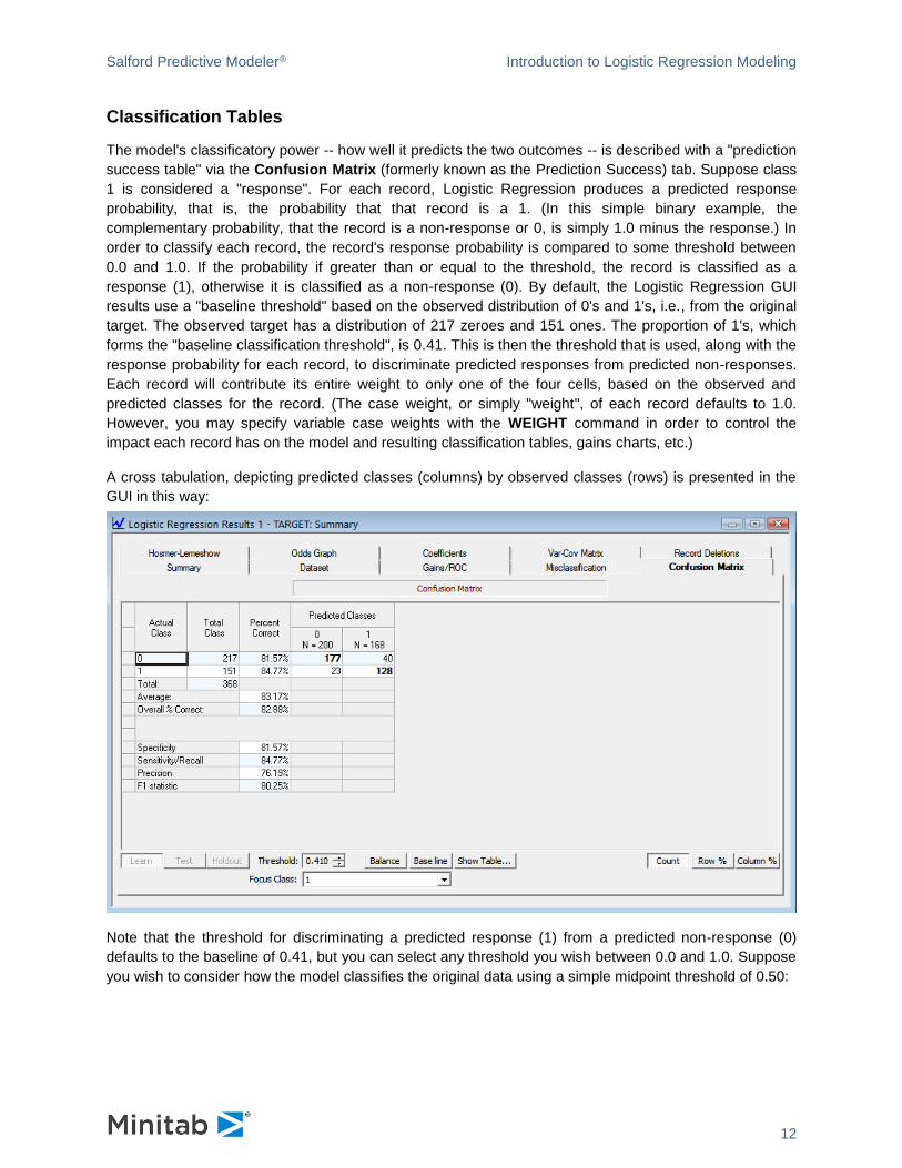
Classification Tables

The model's classificatory power -- how well it predicts the two outcomes -- is described with a "prediction

success table" via the Confusion Matrix (formerly known as the Prediction Success) tab. Suppose class

1 is considered a "response". For each record, Logistic Regression produces a predicted response

probability, that is, the probability that that record is a 1. (In this simple binary example, the

complementary probability, that the record is a non-response or 0, is simply 1.0 minus the response.) In

order to classify each record, the record's response probability is compared to some threshold between

0.0 and 1.0. If the probability if greater than or equal to the threshold, the record is classified as a

response (1), otherwise it is classified as a non-response (0). By default, the Logistic Regression GUI

results use a "baseline threshold" based on the observed distribution of 0's and 1's, i.e., from the original

target. The observed target has a distribution of 217 zeroes and 151 ones. The proportion of 1's, which

forms the "baseline classification threshold", is 0.41. This is then the threshold that is used, along with the

response probability for each record, to discriminate predicted responses from predicted non-responses.

Each record will contribute its entire weight to only one of the four cells, based on the observed and

predicted classes for the record. (The case weight, or simply "weight", of each record defaults to 1.0.

However, you may specify variable case weights with the WEIGHT command in order to control the

impact each record has on the model and resulting classification tables, gains charts, etc.)

A cross tabulation, depicting predicted classes (columns) by observed classes (rows) is presented in the

GUI in this way:

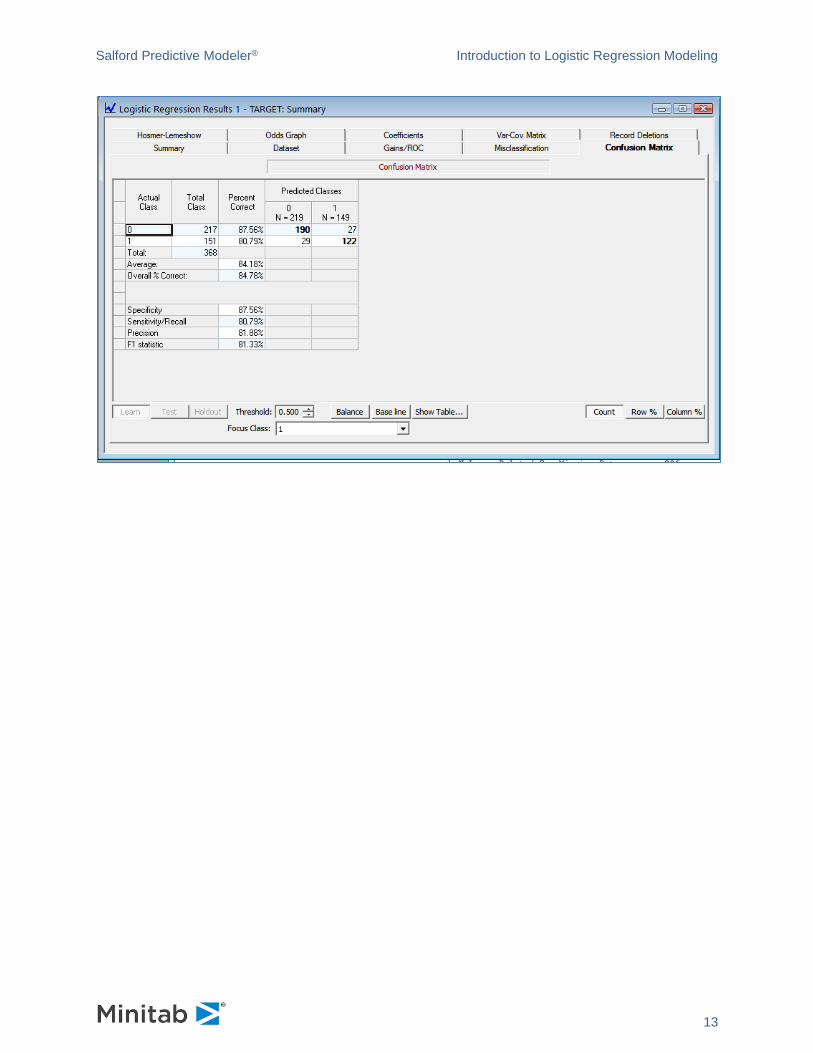
Note that the threshold for discriminating a predicted response (1) from a predicted non-response (0)

defaults to the baseline of 0.41, but you can select any threshold you wish between 0.0 and 1.0. Suppose

you wish to consider how the model classifies the original data using a simple midpoint threshold of 0.50:


13


14

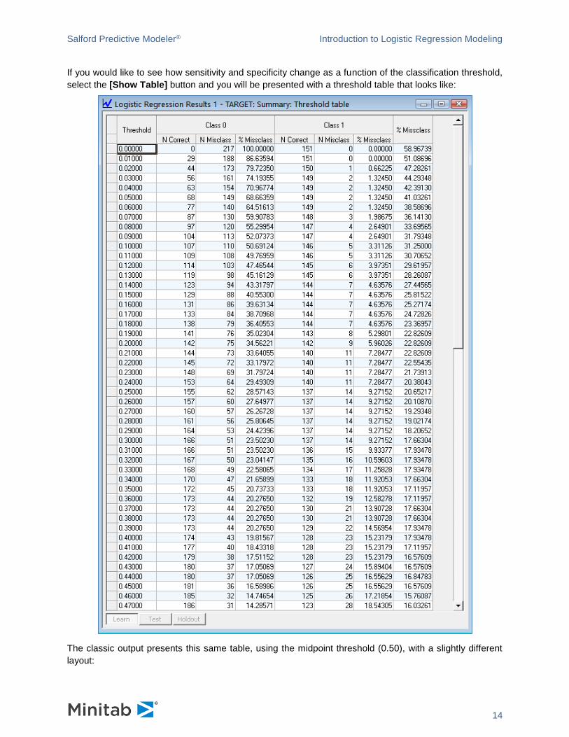
If you would like to see how sensitivity and specificity change as a function of the classification threshold,

select the [Show Table] button and you will be presented with a threshold table that looks like:

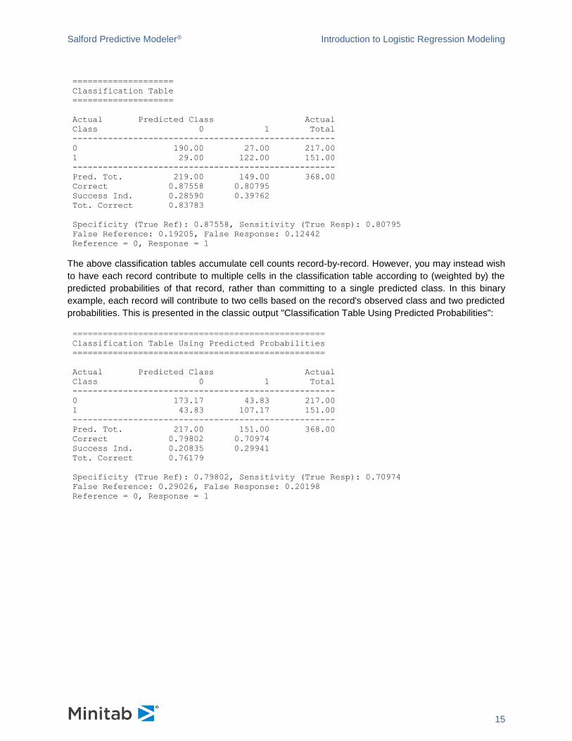
The classic output presents this same table, using the midpoint threshold (0.50), with a slightly different

layout:


15

====================

Classification Table

====================

Actual Predicted Class Actual

Class 0 1 Total

----------------------------------------------------

0 190.00 27.00 217.00

1 29.00 122.00 151.00

----------------------------------------------------

Pred. Tot. 219.00 149.00 368.00

Correct 0.87558 0.80795

Success Ind. 0.28590 0.39762

Tot. Correct 0.83783

Specificity (True Ref): 0.87558, Sensitivity (True Resp): 0.80795

False Reference: 0.19205, False Response: 0.12442

Reference = 0, Response = 1

The above classification tables accumulate cell counts record-by-record. However, you may instead wish

to have each record contribute to multiple cells in the classification table according to (weighted by) the

predicted probabilities of that record, rather than committing to a single predicted class. In this binary

example, each record will contribute to two cells based on the record's observed class and two predicted

probabilities. This is presented in the classic output "Classification Table Using Predicted Probabilities":

==================================================

Classification Table Using Predicted Probabilities

==================================================


Class 0 1 Total

----------------------------------------------------

0 173.17 43.83 217.00

1 43.83 107.17 151.00

----------------------------------------------------

Pred. Tot. 217.00 151.00 368.00

Correct 0.79802 0.70974

Success Ind. 0.20835 0.29941






16

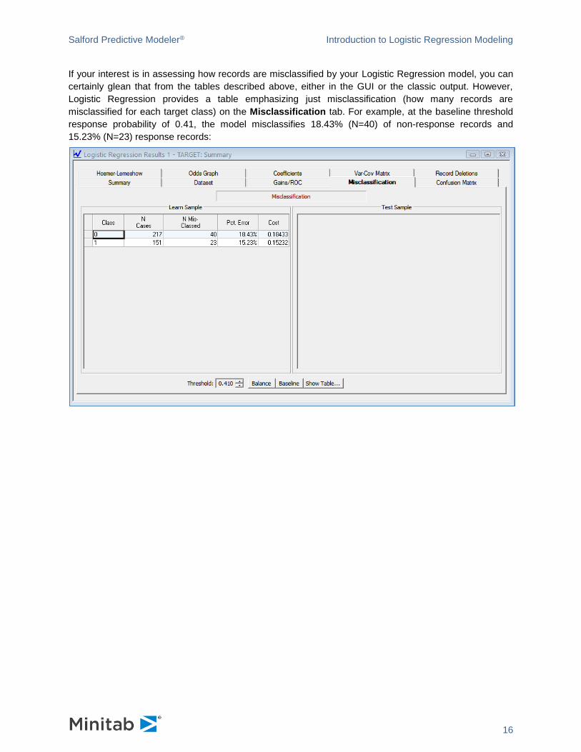
If your interest is in assessing how records are misclassified by your Logistic Regression model, you can

certainly glean that from the tables described above, either in the GUI or the classic output. However,

Logistic Regression provides a table emphasizing just misclassification (how many records are

misclassified for each target class) on the Misclassification tab. For example, at the baseline threshold

response probability of 0.41, the model misclassifies 18.43% (N=40) of non-response records and

15.23% (N=23) response records:


17

A Second Example: Infant Birth Weight

To illustrate the use of binary logistic regression we take some examples from Hosmer and Lemeshow’s

book Applied Logistic Regression, referred to below as H&L. Hosmer and Lemeshow consider data on low

infant birth weight (LOW) as a function of several risk factors. These include the mother’s age (AGE),

mother’s weight during last menstrual period (LWT), race, smoking status during pregnancy (SMOKE),

history of premature labor (PTL), hypertension (HT), uterine irritability (UI), and number of physician visits

during first trimester (FTV). The dependent variable is coded "Low Weight" for birth weights less than

2500g and "Baseline" otherwise. These variables have previously been identified as associated with low

birth weight in the obstetrical literature. A copy of the data appears on the SPM distribution disk as

HOSLEM.CSV (also available as a version referred to as HOSLEM_CHAR.CSV with many variables

preset as categorical variables); the data are reproduced in H&L’s Appendix 1.

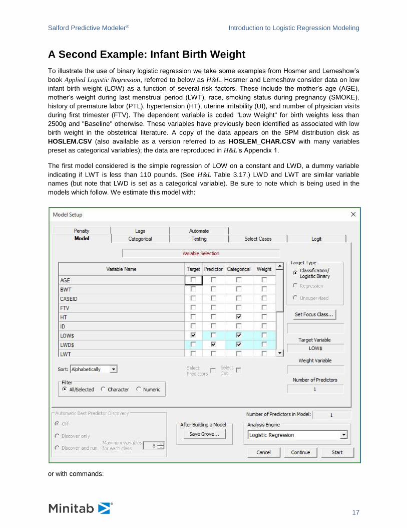
The first model considered is the simple regression of LOW on a constant and LWD, a dummy variable

indicating if LWT is less than 110 pounds. (See H&L Table 3.17.) LWD and LWT are similar variable

names (but note that LWD is set as a categorical variable). Be sure to note which is being used in the

models which follow. We estimate this model with:

or with commands:


18

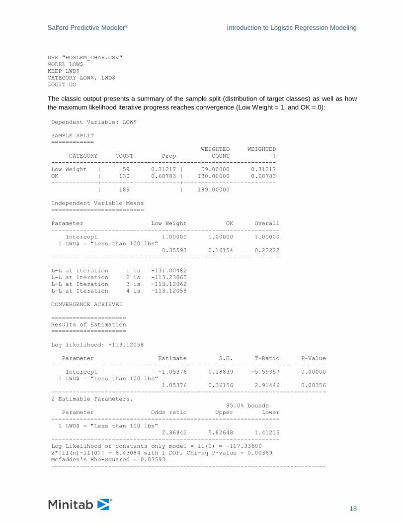
USE "HOSLEM_CHAR.CSV"

MODEL LOW$

KEEP LWD$

CATEGORY LOW$, LWD$

LOGIT GO

The classic output presents a summary of the sample split (distribution of target classes) as well as how

the maximum likelihood iterative progress reaches convergence (Low Weight = 1, and OK = 0):

Dependent Variable: LOW$

SAMPLE SPLIT

============

WEIGHTED WEIGHTED

CATEGORY COUNT Prop COUNT %

---------------------------------------------------------------

Low Weight | 59 0.31217 | 59.00000 0.31217

OK | 130 0.68783 | 130.00000 0.68783

-------------+----------------------+--------------------------

| 189 | 189.00000

Independent Variable Means

==========================

Parameter Low Weight OK Overall

----------------------------------------------------------------

Intercept 1.00000 1.00000 1.00000

1 LWD$ = "Less than 100 lbs"

0.35593 0.16154 0.22222

----------------------------------------------------------------

L-L at Iteration 1 is -131.00482




CONVERGENCE ACHIEVED

=====================


=====================



-----------------------------------------------------------------------------

Intercept -1.05376 0.18839 -5.59357 0.00000


1.05376 0.36156 2.91446 0.00356

-----------------------------------------------------------------------------


95.0% bounds


----------------------------------------------------------------


2.86842 5.82648 1.41215

----------------------------------------------------------------


2*[ll(n)-ll(0)] = 8.43084 with 1 DOF, Chi-sq P-value = 0.00369


-----------------------------------------------------------------------------


19

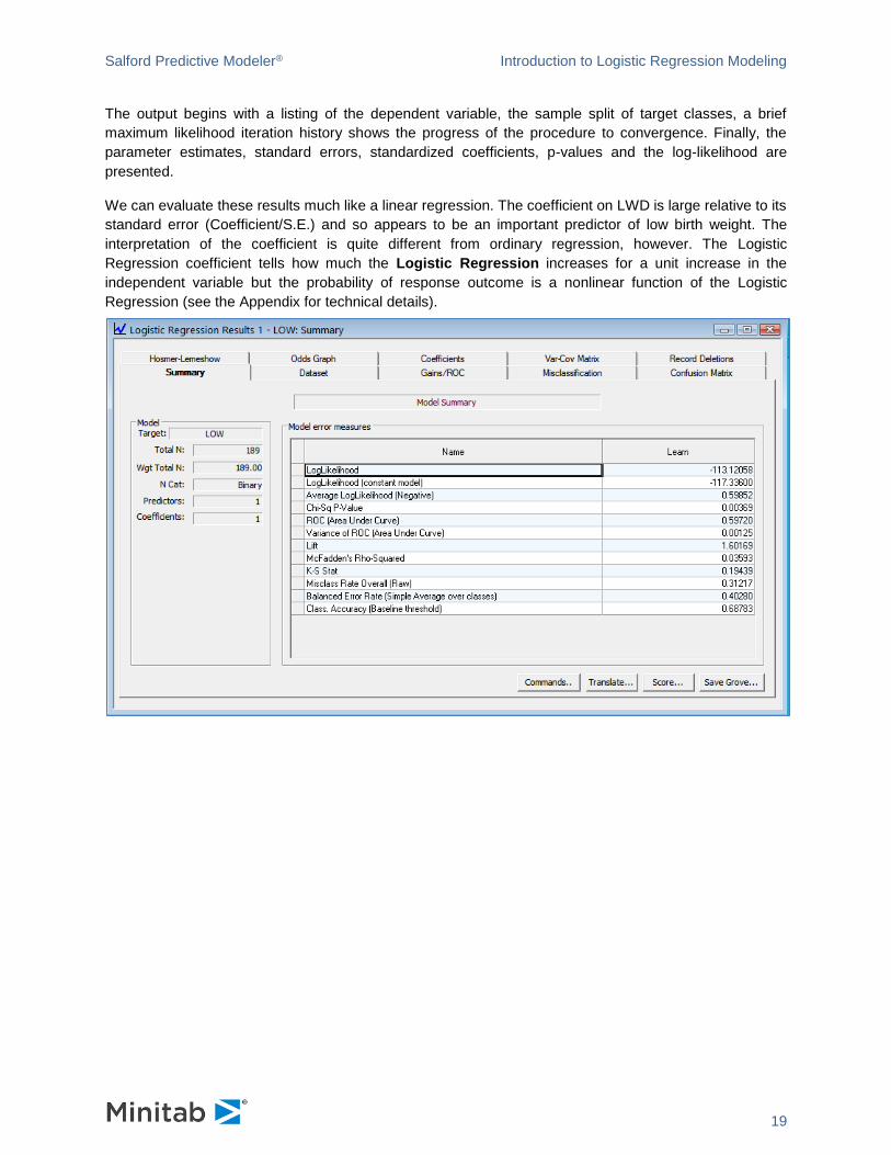
The output begins with a listing of the dependent variable, the sample split of target classes, a brief

maximum likelihood iteration history shows the progress of the procedure to convergence. Finally, the

parameter estimates, standard errors, standardized coefficients, p-values and the log-likelihood are

presented.

We can evaluate these results much like a linear regression. The coefficient on LWD is large relative to its

standard error (Coefficient/S.E.) and so appears to be an important predictor of low birth weight. The

interpretation of the coefficient is quite different from ordinary regression, however. The Logistic

Regression coefficient tells how much the Logistic Regression increases for a unit increase in the

independent variable but the probability of response outcome is a nonlinear function of the Logistic

Regression (see the Appendix for technical details).


20

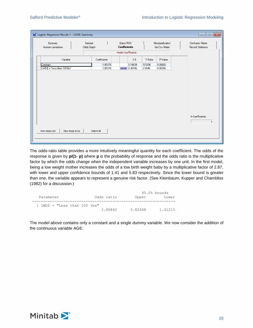
The odds-ratio table provides a more intuitively meaningful quantity for each coefficient. The odds of the

response is given by p/(1- p) where p is the probability of response and the odds ratio is the multiplicative

factor by which the odds change when the independent variable increases by one unit. In the first model,

being a low weight mother increases the odds of a low birth weight baby by a multiplicative factor of 2.87,

with lower and upper confidence bounds of 1.41 and 5.83 respectively. Since the lower bound is greater

than one, the variable appears to represent a genuine risk factor. (See Kleinbaum, Kupper and Chambliss

(1982) for a discussion.)

95.0% bounds


----------------------------------------------------------------


2.86842 5.82648 1.41215

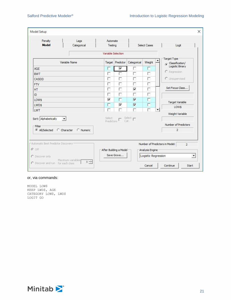
The model above contains only a constant and a single dummy variable. We now consider the addition of

the continuous variable AGE:


21

or, via commands:

MODEL LOW$

KEEP LWD$, AGE

CATEGORY LOW$, LWD$

LOGIT GO


22

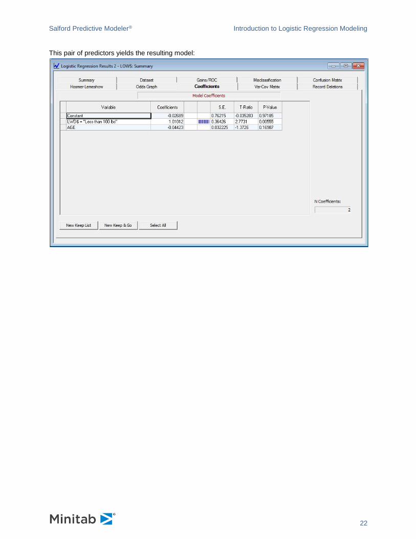
This pair of predictors yields the resulting model:


23


==========================


----------------------------------------------------------------

Intercept 1.00000 1.00000 1.00000

1 LWD$ = "Less than 100 lbs" 0.35593 0.16154

0.22222

2 AGE 22.30508 23.66154 23.23810

----------------------------------------------------------------






=====================


=====================



-----------------------------------------------------------------------------

Intercept -0.02689 0.76215 -0.03528 0.97185


1.01012 0.36426 2.77306 0.00555

2 AGE -0.04423 0.03222 -1.37261 0.16987

-----------------------------------------------------------------------------


95.0% bounds


----------------------------------------------------------------


2.74594 5.60727 1.34471

2 AGE 0.95673 1.01911 0.89817

----------------------------------------------------------------




-----------------------------------------------------------------------------

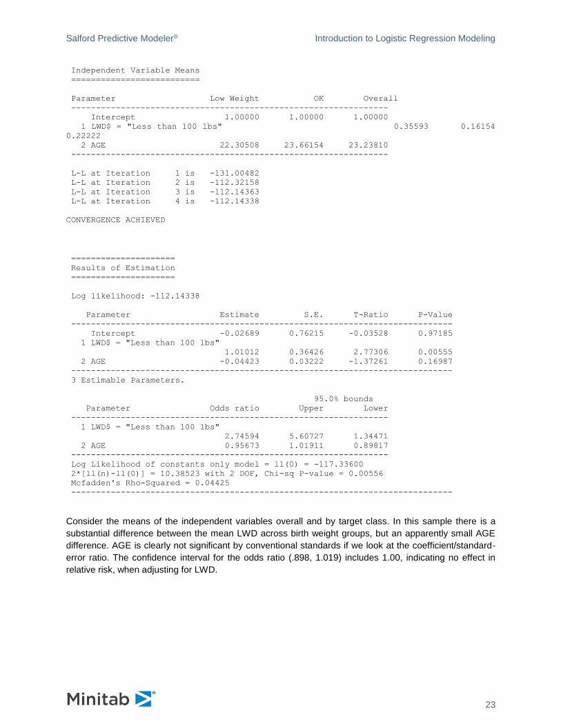
Consider the means of the independent variables overall and by target class. In this sample there is a

substantial difference between the mean LWD across birth weight groups, but an apparently small AGE

difference. AGE is clearly not significant by conventional standards if we look at the coefficient/standard-

error ratio. The confidence interval for the odds ratio (.898, 1.019) includes 1.00, indicating no effect in

relative risk, when adjusting for LWD.


24

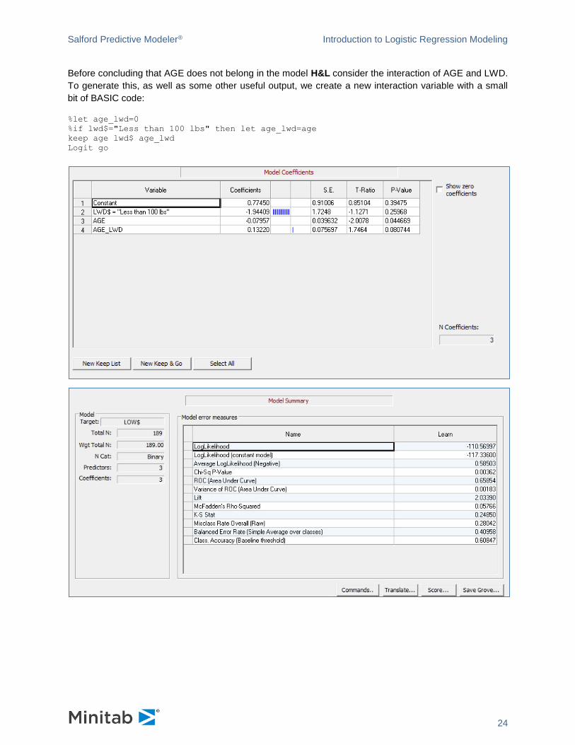
Before concluding that AGE does not belong in the model H&L consider the interaction of AGE and LWD.

To generate this, as well as some other useful output, we create a new interaction variable with a small

bit of BASIC code:

%let age_lwd=0

%if lwd$="Less than 100 lbs" then let age_lwd=age

keep age lwd$ age_lwd

Logit go


25

=====================


=====================



-----------------------------------------------------------------------------

Intercept 0.77450 0.91006 0.85104 0.39475


-1.94409 1.72479 -1.12715 0.25968

2 AGE -0.07957 0.03963 -2.00776 0.04467

3 AGE_LWD 0.13220 0.07570 1.74639 0.08074

-----------------------------------------------------------------------------


95.0% bounds


----------------------------------------------------------------


0.14312 4.20566 0.00487

2 AGE 0.92351 0.99811 0.85449

3 AGE_LWD 1.14133 1.32387 0.98396

----------------------------------------------------------------




-----------------------------------------------------------------------------

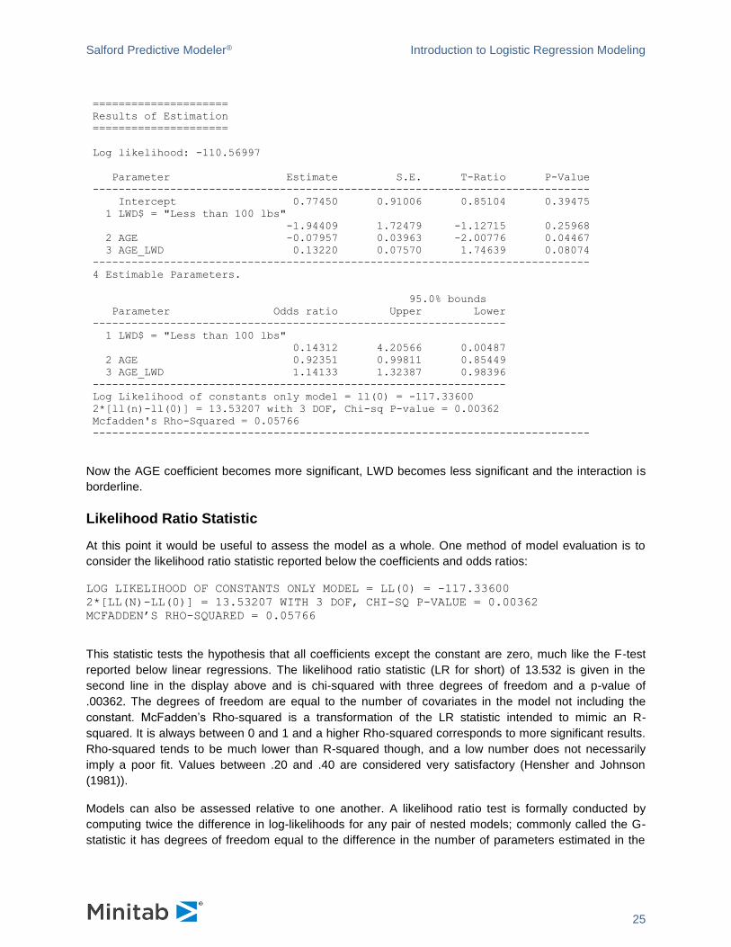
Now the AGE coefficient becomes more significant, LWD becomes less significant and the interaction is

borderline.

Likelihood Ratio Statistic

At this point it would be useful to assess the model as a whole. One method of model evaluation is to

consider the likelihood ratio statistic reported below the coefficients and odds ratios:

LOG LIKELIHOOD OF CONSTANTS ONLY MODEL = LL(0) = -117.33600

2*[LL(N)-LL(0)] = 13.53207 WITH 3 DOF, CHI-SQ P-VALUE = 0.00362

MCFADDEN’S RHO-SQUARED = 0.05766

This statistic tests the hypothesis that all coefficients except the constant are zero, much like the F-test

reported below linear regressions. The likelihood ratio statistic (LR for short) of 13.532 is given in the

second line in the display above and is chi-squared with three degrees of freedom and a p-value of

.00362. The degrees of freedom are equal to the number of covariates in the model not including the

constant. McFadden’s Rho-squared is a transformation of the LR statistic intended to mimic an R-

squared. It is always between 0 and 1 and a higher Rho-squared corresponds to more significant results.

Rho-squared tends to be much lower than R-squared though, and a low number does not necessarily

imply a poor fit. Values between .20 and .40 are considered very satisfactory (Hensher and Johnson

(1981)).

Models can also be assessed relative to one another. A likelihood ratio test is formally conducted by

computing twice the difference in log-likelihoods for any pair of nested models; commonly called the G-

statistic it has degrees of freedom equal to the difference in the number of parameters estimated in the


26

two models. Comparing the current model with the previous model we have

G = 2 * (112.14338 - 110.56997) = 3.14684 with one degree of freedom

which has a p-value of .07607. This result corresponds to the bottom row of H&L’s table 3.17. The

conclusion of the test is that the interaction is borderline significant.

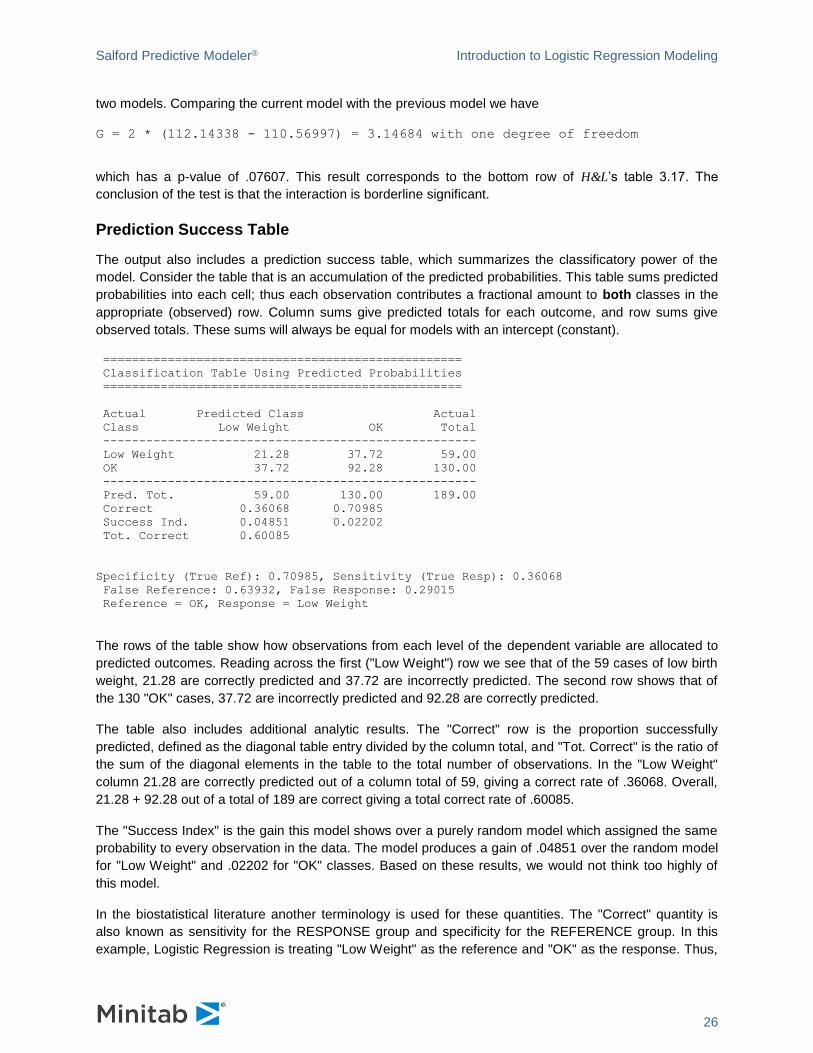
Prediction Success Table

The output also includes a prediction success table, which summarizes the classificatory power of the

model. Consider the table that is an accumulation of the predicted probabilities. This table sums predicted

probabilities into each cell; thus each observation contributes a fractional amount to both classes in the

appropriate (observed) row. Column sums give predicted totals for each outcome, and row sums give

observed totals. These sums will always be equal for models with an intercept (constant).

==================================================

Classification Table Using Predicted Probabilities

==================================================


Class Low Weight OK Total

----------------------------------------------------

Low Weight 21.28 37.72 59.00

OK 37.72 92.28 130.00

----------------------------------------------------

Pred. Tot. 59.00 130.00 189.00

Correct 0.36068 0.70985

Success Ind. 0.04851 0.02202




Reference = OK, Response = Low Weight

The rows of the table show how observations from each level of the dependent variable are allocated to

predicted outcomes. Reading across the first ("Low Weight") row we see that of the 59 cases of low birth

weight, 21.28 are correctly predicted and 37.72 are incorrectly predicted. The second row shows that of

the 130 "OK" cases, 37.72 are incorrectly predicted and 92.28 are correctly predicted.

The table also includes additional analytic results. The "Correct" row is the proportion successfully

predicted, defined as the diagonal table entry divided by the column total, and "Tot. Correct" is the ratio of

the sum of the diagonal elements in the table to the total number of observations. In the "Low Weight"

column 21.28 are correctly predicted out of a column total of 59, giving a correct rate of .36068. Overall,

21.28 + 92.28 out of a total of 189 are correct giving a total correct rate of .60085.

The "Success Index" is the gain this model shows over a purely random model which assigned the same

probability to every observation in the data. The model produces a gain of .04851 over the random model

for "Low Weight" and .02202 for "OK" classes. Based on these results, we would not think too highly of

this model.

In the biostatistical literature another terminology is used for these quantities. The "Correct" quantity is

also known as sensitivity for the RESPONSE group and specificity for the REFERENCE group. In this

example, Logistic Regression is treating "Low Weight" as the reference and "OK" as the response. Thus,


27

sensitivity, associated with response class "OK", is .70985, while specificity, associated with reference

class "Low Weight", is 0.36068. The FALSE REFERENCE rate is the fraction of those predicted to

respond ("OK") that actually did not respond ("Low Weight") while the FALSE RESPONSE rate is the

fraction of those predicted to not respond ("Low Weight") that actually responded ("OK"). We prefer the

Prediction Success terminology because it is applicable to the multinomial case as well (see the

Multinomial Logistic Regression section for further discussion).

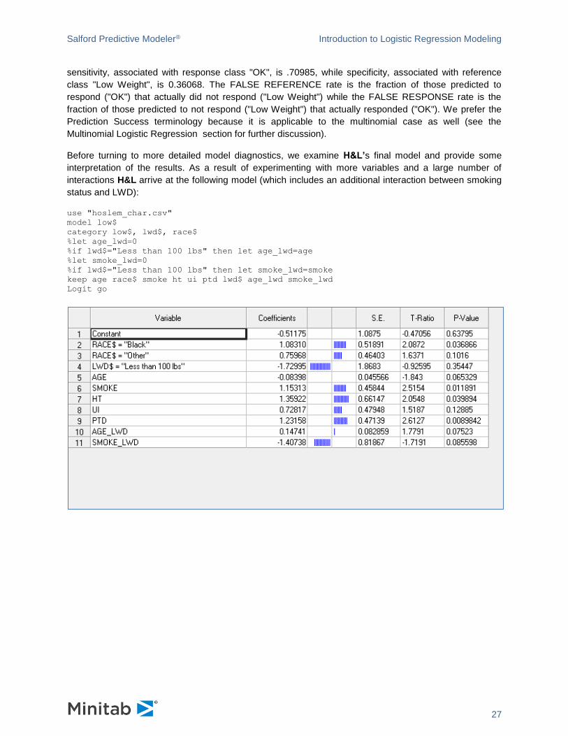
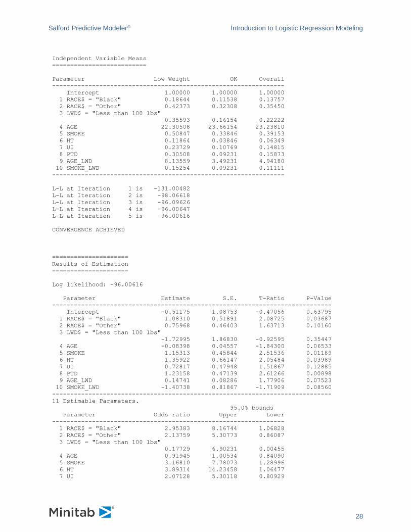
Before turning to more detailed model diagnostics, we examine H&L’s final model and provide some

interpretation of the results. As a result of experimenting with more variables and a large number of

interactions H&L arrive at the following model (which includes an additional interaction between smoking

status and LWD):

use "hoslem_char.csv"

model low$

category low$, lwd$, race$

%let age_lwd=0

%if lwd$="Less than 100 lbs" then let age_lwd=age

%let smoke_lwd=0

%if lwd$="Less than 100 lbs" then let smoke_lwd=smoke

keep age race$ smoke ht ui ptd lwd$ age_lwd smoke_lwd

Logit go


28


==========================


----------------------------------------------------------------

Intercept 1.00000 1.00000 1.00000

1 RACE$ = "Black" 0.18644 0.11538 0.13757

2 RACE$ = "Other" 0.42373 0.32308 0.35450


0.35593 0.16154 0.22222

4 AGE 22.30508 23.66154 23.23810

5 SMOKE 0.50847 0.33846 0.39153

6 HT 0.11864 0.03846 0.06349

7 UI 0.23729 0.10769 0.14815

8 PTD 0.30508 0.09231 0.15873

9 AGE_LWD 8.13559 3.49231 4.94180

10 SMOKE_LWD 0.15254 0.09231 0.11111

----------------------------------------------------------------







=====================


=====================



-----------------------------------------------------------------------------

Intercept -0.51175 1.08753 -0.47056 0.63795

1 RACE$ = "Black" 1.08310 0.51891 2.08725 0.03687

2 RACE$ = "Other" 0.75968 0.46403 1.63713 0.10160


-1.72995 1.86830 -0.92595 0.35447

4 AGE -0.08398 0.04557 -1.84300 0.06533

5 SMOKE 1.15313 0.45844 2.51536 0.01189

6 HT 1.35922 0.66147 2.05484 0.03989

7 UI 0.72817 0.47948 1.51867 0.12885

8 PTD 1.23158 0.47139 2.61266 0.00898

9 AGE_LWD 0.14741 0.08286 1.77906 0.07523

10 SMOKE_LWD -1.40738 0.81867 -1.71909 0.08560

-----------------------------------------------------------------------------


95.0% bounds


----------------------------------------------------------------

1 RACE$ = "Black" 2.95383 8.16744 1.06828

2 RACE$ = "Other" 2.13759 5.30773 0.86087


0.17729 6.90231 0.00455

4 AGE 0.91945 1.00534 0.84090

5 SMOKE 3.16810 7.78073 1.28996

6 HT 3.89314 14.23458 1.06477

7 UI 2.07128 5.30118 0.80929


29

8 PTD 3.42663 8.63207 1.36025

9 AGE_LWD 1.15883 1.36317 0.98512

10 SMOKE_LWD 0.24478 1.21799 0.04920

----------------------------------------------------------------




-----------------------------------------------------------------------------


30

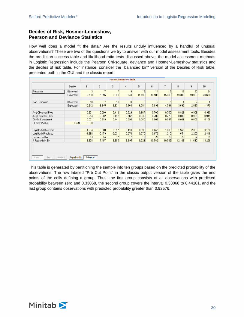
Deciles of Risk, Hosmer-Lemeshow, Pearson and Deviance Statistics

How well does a model fit the data? Are the results unduly influenced by a handful of unusual

observations? These are two of the questions we try to answer with our model assessment tools. Besides

the prediction success table and likelihood ratio tests discussed above, the model assessment methods

in Logistic Regression include the Pearson Chi-square, deviance and Hosmer-Lemeshow statistics and

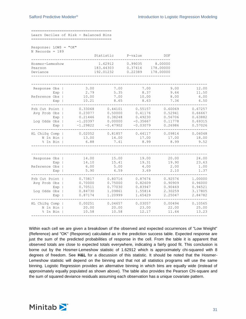
the deciles of risk table. For instance, consider the "balanced bin" version of the Deciles of Risk table,

presented both in the GUI and the classic report:

This table is generated by partitioning the sample into ten groups based on the predicted probability of the

observations. The row labeled "Prb Cut Point" in the classic output version of the table gives the end

points of the cells defining a group. Thus, the first group consists of all observations with predicted

probability between zero and 0.33068, the second group covers the interval 0.33068 to 0.44101, and the

last group contains observations with predicted probability greater than 0.92576.


31

=====================================

Learn Deciles of Risk - Balanced Bins

=====================================

Response: LOW$ = "OK"

N Records = 189

Statistic P-value DOF

----------------------------------------------------------------

Hosmer-Lemeshow 1.62912 0.99035 8.00000

Pearson 183.44303 0.37416 178.00000

Deviance 192.01232 0.22389 178.00000

----------------------------------------------------------------

---------------------------------------------------------------------------------

Response Obs | 3.00 7.00 7.00 9.00 12.00

Exp | 2.79 5.35 8.37 9.64 11.50

Reference Obs | 10.00 7.00 10.00 8.00 6.00

Exp | 10.21 8.65 8.63 7.36 6.50

---------------------------------------------------------------------------------

Prb Cut Point | 0.33068 0.44101 0.55157 0.60069 0.67257

Avg Prob Obs | 0.23077 0.50000 0.41176 0.52941 0.66667

Exp | 0.21446 0.38248 0.49230 0.56706 0.63882

Log Odds Obs | -1.20397 0.00000 -0.35667 0.11778 0.69315

Exp | -1.29822 -0.47902 -0.03079 0.26986 0.57026

---------------------------------------------------------------------------------

HL ChiSq Comp | 0.02052 0.81857 0.44117 0.09814 0.06048

N In Bin | 13.00 14.00 17.00 17.00 18.00

% In Bin | 6.88 7.41 8.99 8.99 9.52

---------------------------------------------------------------------------------

---------------------------------------------------------------------------------

Response Obs | 14.00 15.00 19.00 20.00 24.00

Exp | 14.10 15.41 19.31 19.90 23.63

Reference Obs | 6.00 5.00 4.00 2.00 1.00

Exp | 5.90 4.59 3.69 2.10 1.37

---------------------------------------------------------------------------------

Prb Cut Point | 0.73817 0.80716 0.87674 0.92576 1.00000

Avg Prob Obs | 0.70000 0.75000 0.82609 0.90909 0.96000

Exp | 0.70511 0.77030 0.83947 0.90469 0.94521

Log Odds Obs | 0.84730 1.09861 1.55814 2.30259 3.17805

Exp | 0.87174 1.20999 1.65429 2.25047 2.84782

---------------------------------------------------------------------------------

HL ChiSq Comp | 0.00251 0.04657 0.03057 0.00494 0.10565

N In Bin | 20.00 20.00 23.00 22.00 25.00

% In Bin | 10.58 10.58 12.17 11.64 13.23

---------------------------------------------------------------------------------

Within each cell we are given a breakdown of the observed and expected occurrences of "Low Weight"

(Reference) and "OK" (Response) calculated as in the prediction success table. Expected response are

just the sum of the predicted probabilities of response in the cell. From the table it is apparent that

observed totals are close to expected totals everywhere, indicating a fairly good fit. This conclusion is

borne out by the Hosmer-Lemeshow statistic of 1.62912 which is approximately chi-squared with 8

degrees of freedom. See H&L for a discussion of this statistic. It should be noted that the Hosmer-

Lemeshow statistic will depend on the binning and that not all statistics programs will use the same

binning. Logistic Regression provides an alternative binning in which bins are equally wide (instead of

approximately equally populated as shown above). The table also provides the Pearson Chi-square and

the sum of squared deviance residuals assuming each observation has a unique covariate pattern.


32

Multinomial Logistic Regression

The multinomial logistic regression is a logistic regression model having a dependent variable with more

than two levels (Agresti (1990), Santer and Duffy (1989), Nerlove and Press (1973)). Examples of such

dependent variables include political preference (Democrat, Republican, Independent), health status

(healthy, moderately impaired, seriously impaired), smoking status (current smoker, former smoker, never

smoked), and job classification (executive, manager, technical staff, clerical, other). Outside of the

difference in the number of levels of the dependent variable, the multinomial logistic regression is very

similar to the binary logistic regression and most of the previously discussed tools of interpretation,

analysis, and model selection can be applied. In fact, the polytomous unordered logistic regression we

discuss here is essentially a combination of several binary logistic regressions estimated simultaneously

(Begg and Gray (1984)). We use the term polytomous to differentiate this model from the conditional

logistic regression and discrete choice models available in separate software from Salford Systems.

There are important differences between binary and multinomial models however. Chiefly, the multinomial

output is more complicated than that of the binary model, and care must be taken in the interpretation of

the results. Fortunately, Logistic Regression provides tools which make the task of interpretation much

easier. There is also a difference in dependent variable coding. The binary logistic regression dependent

variable is normally coded 0 or 1 (but can be any two distinct values), whereas the multinomial dependent

is often coded 1,2,...,K (but can be any K distinct values).

We will illustrate multinomial modeling with an example, emphasizing what is new in this context. If you

have not already read the section on binary logistic regression, this is a good time to do so.

Example

The data used below have been extracted from the National Longitudinal Survey of Young Men, 1979.

Information on 200 individuals is supplied on school enrollment status (NOTENR=1 if not enrolled, 0

otherwise), base-10 log of wage (LW), age, highest completed grade (EDUC), mother’s education (MED),

father’s education (FED), an index of reading material available in the home (CULTURE=1 for least, 3 for

most), mean income of persons in father’s occupation in 1960 (FOMY), an IQ measure, a race dummy

(BLACK=0 for white), a region dummy (SOUTH=0 for non-South) and the number of siblings (NSIBS).

The data appear in the SPM installation files as NLS.CSV. We estimate a model to analyze the

CULTURE variable, predicting its value with several demographic characteristics. In this example, we

ignore the fact that the dependent variable is ordinal and treat it as a nominal variable. (See Agresti

(1990) for a discussion of the distinction.)


33

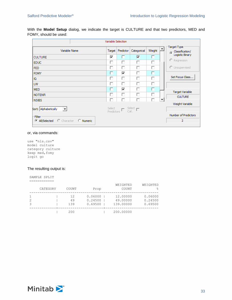
With the Model Setup dialog, we indicate the target is CULTURE and that two predictors, MED and

FOMY, should be used:

or, via commands:

use "nls.csv"

model culture

category culture

keep med,fomy

logit go

The resulting output is:

SAMPLE SPLIT

============

WEIGHTED WEIGHTED

CATEGORY COUNT Prop COUNT %

---------------------------------------------------------------

1 | 12 0.06000 | 12.00000 0.06000

2 | 49 0.24500 | 49.00000 0.24500

3 | 139 0.69500 | 139.00000 0.69500

-------------+----------------------+--------------------------

| 200 | 200.00000


34


==========================

Parameter 1 2 3 Overall

-----------------------------------------------------------------------------

Intercept 1.00000 1.00000 1.00000 1.00000

1 MED 8.75000 10.18367 11.44604 10.97500

2 FOMY 4551.50000 5368.85714 6116.13669 5839.17500

-----------------------------------------------------------------------------








=====================


=====================



-----------------------------------------------------------------------------

Choice group: 1

Intercept 5.06375 1.69634 2.98511 0.00283

1 MED -0.42277 0.14229 -2.97118 0.00297

2 FOMY -0.00062 0.00024 -2.60343 0.00923

Choice group: 2

Intercept 2.54345 0.98338 2.58643 0.00970

1 MED -0.19172 0.07682 -2.49562 0.01257

2 FOMY -0.00026 0.00012 -2.18842 0.02864

-----------------------------------------------------------------------------


95.0% bounds


----------------------------------------------------------------

Choice group: 1

1 MED 0.65523 0.86599 0.49577

2 FOMY 0.99938 0.99985 0.99892

Choice group: 2

1 MED 0.82554 0.95969 0.71015

2 FOMY 0.99974 0.99997 0.99950

----------------------------------------------------------------


2*[ll(n)-ll(0)] = 30.93787 with 4 DOF, Chi-Sq P-value = 0.00000


-----------------------------------------------------------------------------

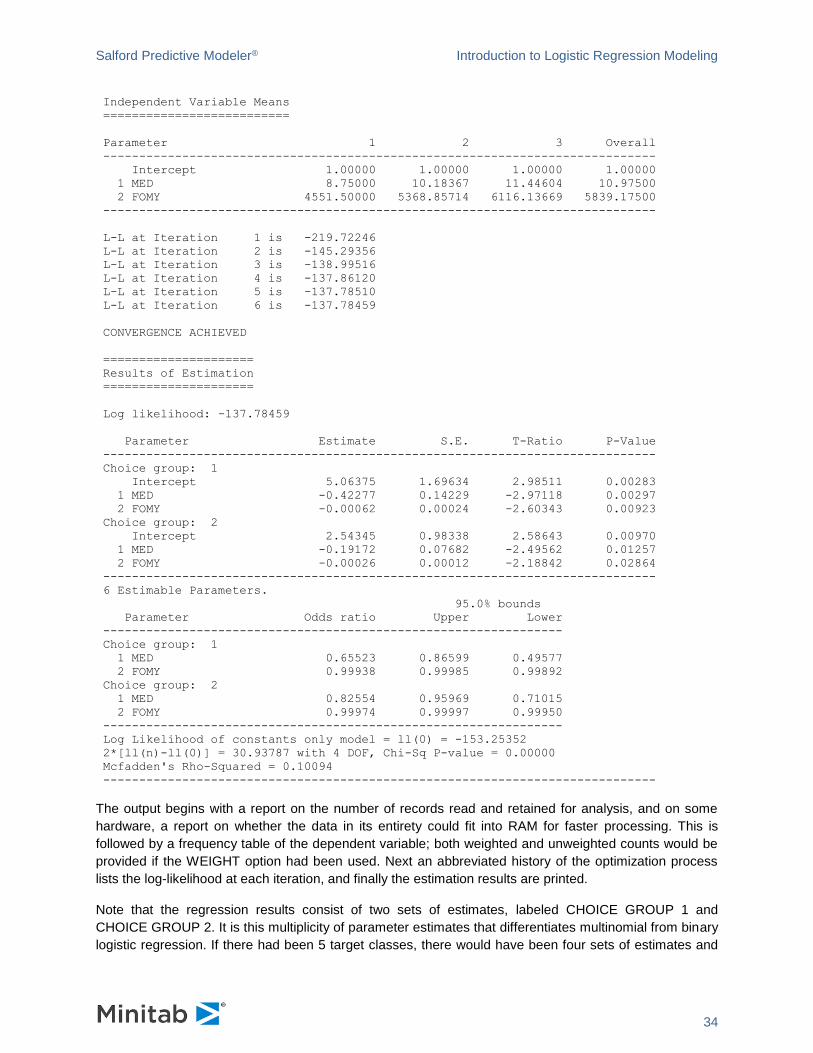
The output begins with a report on the number of records read and retained for analysis, and on some

hardware, a report on whether the data in its entirety could fit into RAM for faster processing. This is

followed by a frequency table of the dependent variable; both weighted and unweighted counts would be

provided if the WEIGHT option had been used. Next an abbreviated history of the optimization process

lists the log-likelihood at each iteration, and finally the estimation results are printed.

Note that the regression results consist of two sets of estimates, labeled CHOICE GROUP 1 and

CHOICE GROUP 2. It is this multiplicity of parameter estimates that differentiates multinomial from binary

logistic regression. If there had been 5 target classes, there would have been four sets of estimates and


35

in general there are NClasses - 1 sets of coefficients.

This volume of output provides the challenge to understanding the results. The output is a little more

intelligible when you realize that we have really estimated a series of binary logistic regressions

simultaneously. The first sub-model consists of the two dependent variable categories 1 and 3 and the

second consists of categories 2 and 3. These sub-models always include the highest level of the

dependent variable as the reference class and one other level as the response class.

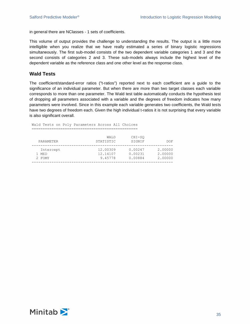
Wald Tests

The coefficient/standard-error ratios ("t-ratios") reported next to each coefficient are a guide to the

significance of an individual parameter. But when there are more than two target classes each variable

corresponds to more than one parameter. The Wald test table automatically conducts the hypothesis test

of dropping all parameters associated with a variable and the degrees of freedom indicates how many

parameters were involved. Since in this example each variable generates two coefficients, the Wald tests

have two degrees of freedom each. Given the high individual t-ratios it is not surprising that every variable

is also significant overall.

Wald Tests on Poly Parameters Across All Choices

================================================

WALD CHI-SQ

PARAMETER STATISTIC SIGNIF DOF

----------------------------------------------------------------

Intercept 12.00309 0.00247 2.00000

1 MED 12.14107 0.00231 2.00000

2 FOMY 9.45778 0.00884 2.00000

----------------------------------------------------------------


36

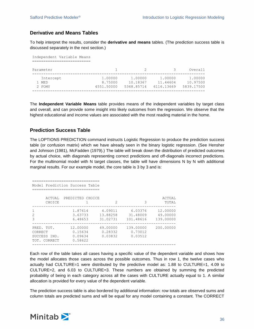
Derivative and Means Tables

To help interpret the results, consider the derivative and means tables. (The prediction success table is

discussed separately in the next section.)


==========================


-----------------------------------------------------------------------------

Intercept 1.00000 1.00000 1.00000 1.00000

1 MED 8.75000 10.18367 11.44604 10.97500

2 FOMY 4551.50000 5368.85714 6116.13669 5839.17500

-----------------------------------------------------------------------------

The Independent Variable Means table provides means of the independent variables by target class

and overall, and can provide some insight into likely outcomes from the regression. We observe that the

highest educational and income values are associated with the most reading material in the home.

Prediction Success Table

The LOPTIONS PREDICTION command instructs Logistic Regression to produce the prediction success

table (or confusion matrix) which we have already seen in the binary logistic regression. (See Hensher

and Johnson (1981), McFadden (1979).) The table will break down the distribution of predicted outcomes

by actual choice, with diagonals representing correct predictions and off-diagonals incorrect predictions.

For the multinomial model with N target classes, the table will have dimensions N by N with additional

marginal results. For our example model, the core table is 3 by 3 and is:

==============================

Model Prediction Success Table

==============================

ACTUAL PREDICTED CHOICE ACTUAL

CHOICE 1 2 3 TOTAL

----------------------------------------------------------------

1 1.87614 4.09011 6.03376 12.00000

2 3.63733 13.88258 31.48009 49.00000

3 6.48653 31.02731 101.48616 139.00000

----------------------------------------------------------------

PRED. TOT. 12.00000 49.00000 139.00000 200.00000

CORRECT 0.15634 0.28332 0.73012

SUCCESS IND. 0.09634 0.03832 0.03512

TOT. CORRECT 0.58622

----------------------------------------------------------------

Each row of the table takes all cases having a specific value of the dependent variable and shows how

the model allocates those cases across the possible outcomes. Thus in row 1, the twelve cases who

actually had CULTURE=1 were distributed by the predictive model as: 1.88 to CULTURE=1, 4.09 to

CULTURE=2, and 6.03 to CULTURE=3. These numbers are obtained by summing the predicted

probability of being in each category across all the cases with CULTURE actually equal to 1. A similar

allocation is provided for every value of the dependent variable.

The prediction success table is also bordered by additional information: row totals are observed sums and

column totals are predicted sums and will be equal for any model containing a constant. The CORRECT


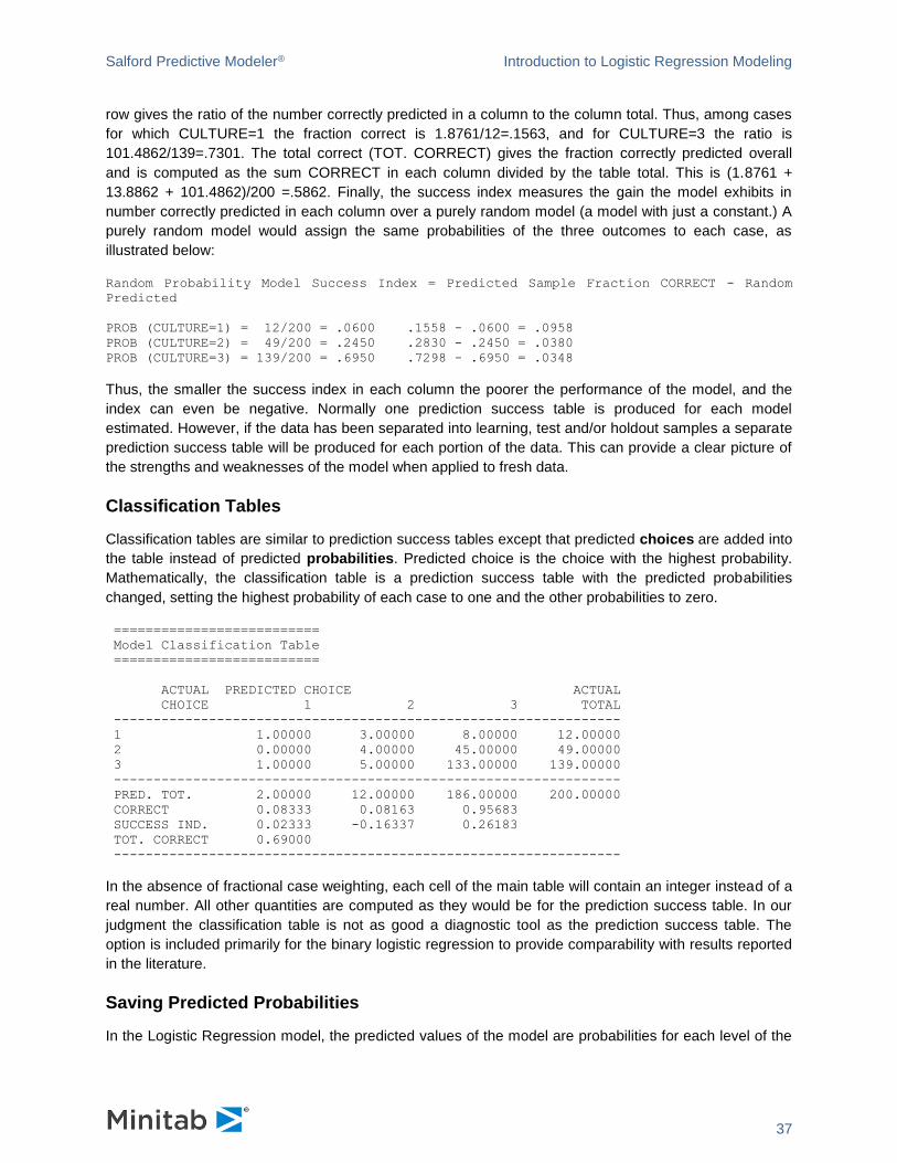
37

row gives the ratio of the number correctly predicted in a column to the column total. Thus, among cases

for which CULTURE=1 the fraction correct is 1.8761/12=.1563, and for CULTURE=3 the ratio is

101.4862/139=.7301. The total correct (TOT. CORRECT) gives the fraction correctly predicted overall

and is computed as the sum CORRECT in each column divided by the table total. This is (1.8761 +

13.8862 + 101.4862)/200 =.5862. Finally, the success index measures the gain the model exhibits in

number correctly predicted in each column over a purely random model (a model with just a constant.) A

purely random model would assign the same probabilities of the three outcomes to each case, as

illustrated below:

Random Probability Model Success Index = Predicted Sample Fraction CORRECT - Random

Predicted

PROB (CULTURE=1) = 12/200 = .0600 .1558 - .0600 = .0958

PROB (CULTURE=2) = 49/200 = .2450 .2830 - .2450 = .0380

PROB (CULTURE=3) = 139/200 = .6950 .7298 - .6950 = .0348

Thus, the smaller the success index in each column the poorer the performance of the model, and the

index can even be negative. Normally one prediction success table is produced for each model

estimated. However, if the data has been separated into learning, test and/or holdout samples a separate

prediction success table will be produced for each portion of the data. This can provide a clear picture of

the strengths and weaknesses of the model when applied to fresh data.

Classification Tables

Classification tables are similar to prediction success tables except that predicted choices are added into

the table instead of predicted probabilities. Predicted choice is the choice with the highest probability.

Mathematically, the classification table is a prediction success table with the predicted probabilities

changed, setting the highest probability of each case to one and the other probabilities to zero.

==========================

Model Classification Table

==========================

ACTUAL PREDICTED CHOICE ACTUAL

CHOICE 1 2 3 TOTAL

----------------------------------------------------------------

1 1.00000 3.00000 8.00000 12.00000

2 0.00000 4.00000 45.00000 49.00000

3 1.00000 5.00000 133.00000 139.00000

----------------------------------------------------------------

PRED. TOT. 2.00000 12.00000 186.00000 200.00000

CORRECT 0.08333 0.08163 0.95683

SUCCESS IND. 0.02333 -0.16337 0.26183

TOT. CORRECT 0.69000

----------------------------------------------------------------

In the absence of fractional case weighting, each cell of the main table will contain an integer instead of a

real number. All other quantities are computed as they would be for the prediction success table. In our

judgment the classification table is not as good a diagnostic tool as the prediction success table. The

option is included primarily for the binary logistic regression to provide comparability with results reported

in the literature.

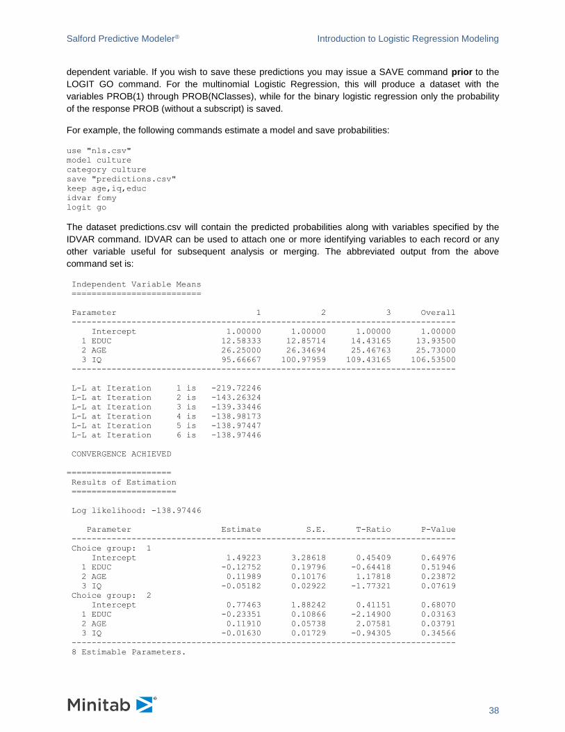
Saving Predicted Probabilities

In the Logistic Regression model, the predicted values of the model are probabilities for each level of the


38

dependent variable. If you wish to save these predictions you may issue a SAVE command prior to the

LOGIT GO command. For the multinomial Logistic Regression, this will produce a dataset with the

variables PROB(1) through PROB(NClasses), while for the binary logistic regression only the probability

of the response PROB (without a subscript) is saved.

For example, the following commands estimate a model and save probabilities:

use "nls.csv"

model culture

category culture

save "predictions.csv"

keep age,iq,educ

idvar fomy

logit go

The dataset predictions.csv will contain the predicted probabilities along with variables specified by the

IDVAR command. IDVAR can be used to attach one or more identifying variables to each record or any

other variable useful for subsequent analysis or merging. The abbreviated output from the above

command set is:


==========================


-----------------------------------------------------------------------------

Intercept 1.00000 1.00000 1.00000 1.00000

1 EDUC 12.58333 12.85714 14.43165 13.93500

2 AGE 26.25000 26.34694 25.46763 25.73000

3 IQ 95.66667 100.97959 109.43165 106.53500

-----------------------------------------------------------------------------








=====================


=====================



-----------------------------------------------------------------------------

Choice group: 1

Intercept 1.49223 3.28618 0.45409 0.64976

1 EDUC -0.12752 0.19796 -0.64418 0.51946

2 AGE 0.11989 0.10176 1.17818 0.23872

3 IQ -0.05182 0.02922 -1.77321 0.07619

Choice group: 2

Intercept 0.77463 1.88242 0.41151 0.68070

1 EDUC -0.23351 0.10866 -2.14900 0.03163

2 AGE 0.11910 0.05738 2.07581 0.03791

3 IQ -0.01630 0.01729 -0.94305 0.34566

-----------------------------------------------------------------------------



39

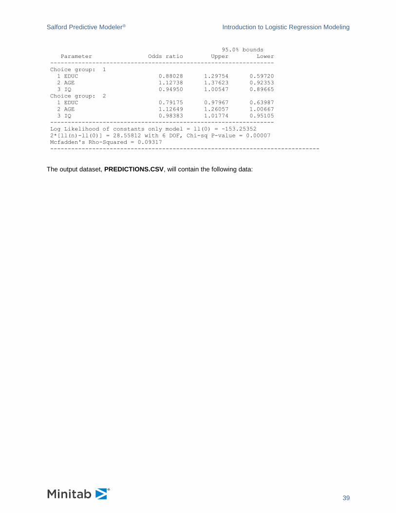
95.0% bounds


----------------------------------------------------------------

Choice group: 1

1 EDUC 0.88028 1.29754 0.59720

2 AGE 1.12738 1.37623 0.92353

3 IQ 0.94950 1.00547 0.89665

Choice group: 2

1 EDUC 0.79175 0.97967 0.63987

2 AGE 1.12649 1.26057 1.00667

3 IQ 0.98383 1.01774 0.95105

----------------------------------------------------------------




-----------------------------------------------------------------------------

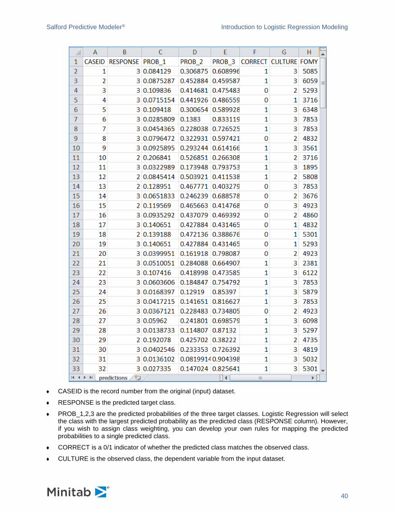
The output dataset, PREDICTIONS.CSV, will contain the following data:


40

CASEID is the record number from the original (input) dataset.

RESPONSE is the predicted target class.

PROB_1,2,3 are the predicted probabilities of the three target classes. Logistic Regression will select the class with the largest predicted probability as the predicted class (RESPONSE column). However, if you wish to assign class weighting, you can develop your own rules for mapping the predicted probabilities to a single predicted class.

CORRECT is a 0/1 indicator of whether the predicted class matches the observed class.

CULTURE is the observed class, the dependent variable from the input dataset.


41

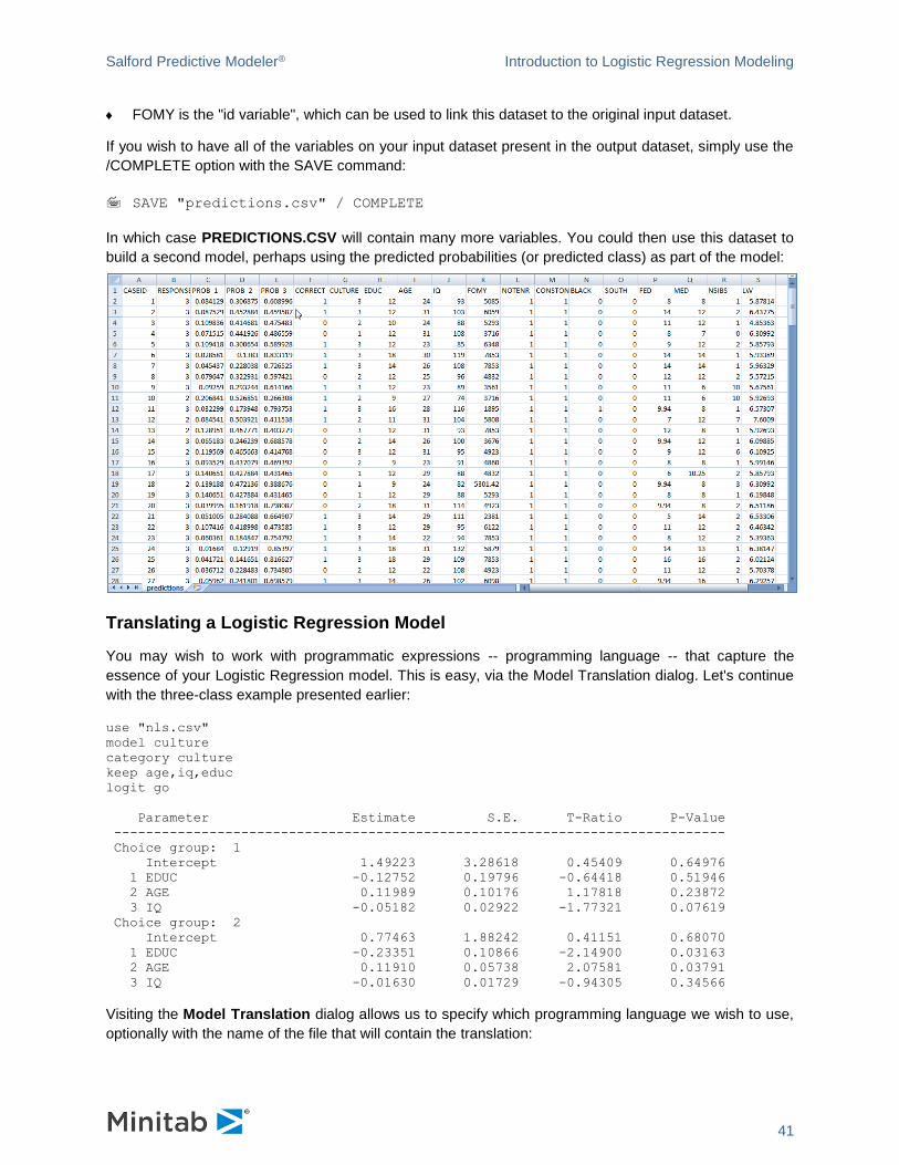
FOMY is the "id variable", which can be used to link this dataset to the original input dataset.

If you wish to have all of the variables on your input dataset present in the output dataset, simply use the

/COMPLETE option with the SAVE command:

SAVE "predictions.csv" / COMPLETE

In which case PREDICTIONS.CSV will contain many more variables. You could then use this dataset to

build a second model, perhaps using the predicted probabilities (or predicted class) as part of the model:

Translating a Logistic Regression Model

You may wish to work with programmatic expressions -- programming language -- that capture the

essence of your Logistic Regression model. This is easy, via the Model Translation dialog. Let's continue

with the three-class example presented earlier:

use "nls.csv"

model culture

category culture

keep age,iq,educ

logit go


-----------------------------------------------------------------------------

Choice group: 1

Intercept 1.49223 3.28618 0.45409 0.64976

1 EDUC -0.12752 0.19796 -0.64418 0.51946

2 AGE 0.11989 0.10176 1.17818 0.23872

3 IQ -0.05182 0.02922 -1.77321 0.07619

Choice group: 2

Intercept 0.77463 1.88242 0.41151 0.68070

1 EDUC -0.23351 0.10866 -2.14900 0.03163

2 AGE 0.11910 0.05738 2.07581 0.03791

3 IQ -0.01630 0.01729 -0.94305 0.34566

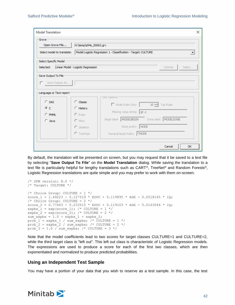
Visiting the Model Translation dialog allows us to specify which programming language we wish to use,

optionally with the name of the file that will contain the translation:


42

By default, the translation will be presented on screen, but you may request that it be saved to a text file

by selecting "Save Output To File" on the Model Translation dialog. While saving the translation to a

text file is particularly helpful for lengthy translations such as CART®, TreeNet® and Random Forests®,

Logistic Regression translations are quite simple and you may prefer to work with them on-screen:

/* SPM version: 8.0 */

/* Target: CULTURE */

/* Choice Group: CULTURE = 1 */

score_1 = 1.49223 - 0.127519 * EDUC + 0.119895 * AGE - 0.0518165 * IQ;

/* Choice Group: CULTURE = 2 */

score_2 = 0.77463 - 0.233515 * EDUC + 0.119103 * AGE - 0.0163044 * IQ;

expbx_1 = exp(score_1); /* CULTURE = 1 */

expbx_2 = exp(score_2); /* CULTURE = 2 */

sum_expbx = 1.0 + expbx_1 + expbx_2;

prob_1 = expbx_1 / sum_expbx; /* CULTURE = 1 */

prob_2 = expbx_2 / sum_expbx; /* CULTURE = 2 */

prob_3 = 1.0 / sum_expbx; /* CULTURE = 3 */

Note that the model coefficients lead to two scores for target classes CULTURE=1 and CULTURE=2,

while the third target class is "left out". This left out class is characteristic of Logistic Regression models.

The expressions are used to produce a score for each of the first two classes, which are then

exponentiated and normalized to produce predicted probabilities.

Using an Independent Test Sample

You may have a portion of your data that you wish to reserve as a test sample. In this case, the test


43

sample records will have no influence on the model estimation, but performance measures for the test

sample will be computed and presented alongside comparable measures based on the learning sample.

Let's consider a dataset concerning "spam" email named SPAMBASE.CSV (or SPAM.CSV). The

dependent variable SPAM is 1 if an email was considered spam by the research team that assembled the

dataset, and 0 if not. In other words, an incoming email that receives a predicted class of 1 is an email

with which we would not want to be bothered, while instead we wish to have all the emails that are

predicted to be of class 0 reach our inbox. A variety of predictive variables are available on the dataset,

and most are used in this example but not explained in detail. In addition, the variable TESTVAR is

provided which takes on values 0 and 1. We would like the SPM will treat records with TESTVAR=1 as a

test sample, such that they are processed and available for model performance evaluation but are not

actually used in the model estimation itself. In this was we not only can see how the model performs in

terms of classification performance on the data with which it was built but we can also see how it performs

on data the model has never seen before.

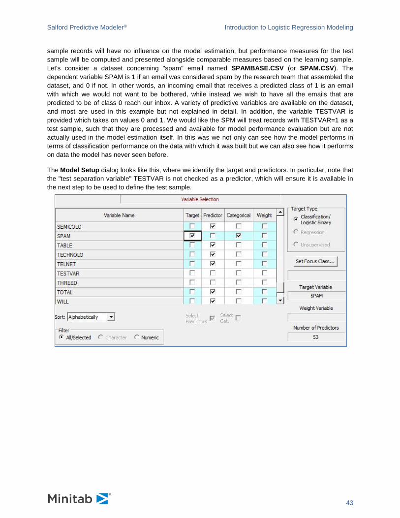
The Model Setup dialog looks like this, where we identify the target and predictors. In particular, note that

the "test separation variable" TESTVAR is not checked as a predictor, which will ensure it is available in

the next step to be used to define the test sample.


44

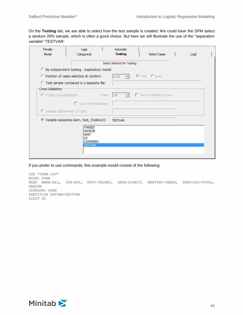
On the Testing tab, we are able to select how the test sample is created. We could have the SPM select

a random 20% sample, which is often a good choice. But here we will illustrate the use of the "separation

variable" TESTVAR:

If you prefer to use commands, this example would consist of the following:

USE "SPAM.CSV"

MODEL SPAM

KEEP MAKE-ALL, OUR-HPL, N650-TELNET, DATA-DIRECT, MEETING-TABLE, SEMICOLO-TOTAL,

RANDOM

CATEGORY SPAM

PARTITION SEPVAR=TESTVAR

LOGIT GO


45

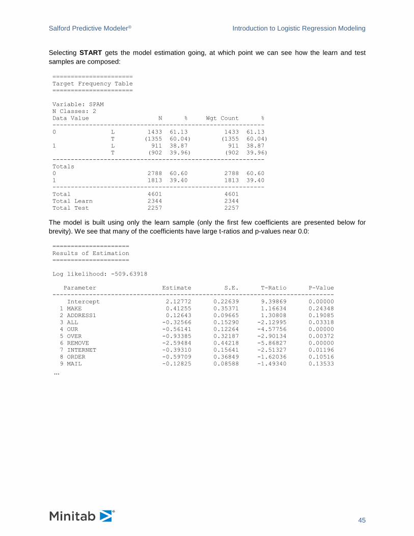
Selecting START gets the model estimation going, at which point we can see how the learn and test

samples are composed:

======================

Target Frequency Table

======================

Variable: SPAM

N Classes: 2

Data Value N % Wgt Count %

----------------------------------------------------------

0 L 1433 61.13 1433 61.13

T (1355 60.04) (1355 60.04)

1 L 911 38.87 911 38.87

T (902 39.96) (902 39.96)

----------------------------------------------------------

Totals

0 2788 60.60 2788 60.60

1 1813 39.40 1813 39.40

----------------------------------------------------------

Total 4601 4601

Total Learn 2344 2344

Total Test 2257 2257

The model is built using only the learn sample (only the first few coefficients are presented below for

brevity). We see that many of the coefficients have large t-ratios and p-values near 0.0:

=====================


=====================



-----------------------------------------------------------------------------

Intercept 2.12772 0.22639 9.39869 0.00000

1 MAKE 0.41255 0.35371 1.16634 0.24348

2 ADDRESS1 0.12643 0.09665 1.30808 0.19085

3 ALL -0.32566 0.15290 -2.12995 0.03318

4 OUR -0.56141 0.12264 -4.57756 0.00000

5 OVER -0.93385 0.32187 -2.90134 0.00372

6 REMOVE -2.59484 0.44218 -5.86827 0.00000

7 INTERNET -0.39310 0.15641 -2.51327 0.01196

8 ORDER -0.59709 0.36849 -1.62036 0.10516

9 MAIL -0.12825 0.08588 -1.49340 0.13533

...


46

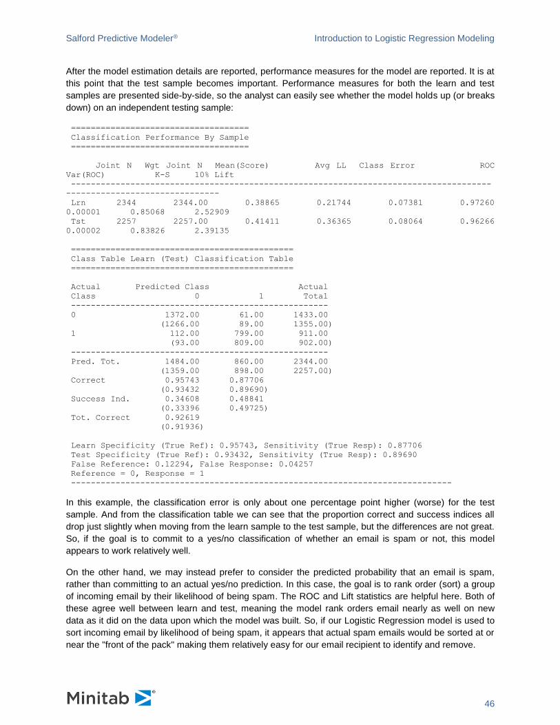
After the model estimation details are reported, performance measures for the model are reported. It is at

this point that the test sample becomes important. Performance measures for both the learn and test

samples are presented side-by-side, so the analyst can easily see whether the model holds up (or breaks

down) on an independent testing sample:

====================================

Classification Performance By Sample

====================================

Joint N Wgt Joint N Mean(Score) Avg LL Class Error ROC

Var(ROC) K-S 10% Lift

-------------------------------------------------------------------------------------

-------------------------------

Lrn 2344 2344.00 0.38865 0.21744 0.07381 0.97260

0.00001 0.85068 2.52909

Tst 2257 2257.00 0.41411 0.36365 0.08064 0.96266

0.00002 0.83826 2.39135

=============================================

Class Table Learn (Test) Classification Table

=============================================


Class 0 1 Total

----------------------------------------------------

0 1372.00 61.00 1433.00

(1266.00 89.00 1355.00)

1 112.00 799.00 911.00

(93.00 809.00 902.00)

----------------------------------------------------

Pred. Tot. 1484.00 860.00 2344.00

(1359.00 898.00 2257.00)

Correct 0.95743 0.87706

(0.93432 0.89690)

Success Ind. 0.34608 0.48841

(0.33396 0.49725)


(0.91936)

Learn Specificity (True Ref): 0.95743, Sensitivity (True Resp): 0.87706

Test Specificity (True Ref): 0.93432, Sensitivity (True Resp): 0.89690



-----------------------------------------------------------------------------

In this example, the classification error is only about one percentage point higher (worse) for the test

sample. And from the classification table we can see that the proportion correct and success indices all

drop just slightly when moving from the learn sample to the test sample, but the differences are not great.

So, if the goal is to commit to a yes/no classification of whether an email is spam or not, this model

appears to work relatively well.

On the other hand, we may instead prefer to consider the predicted probability that an email is spam,

rather than committing to an actual yes/no prediction. In this case, the goal is to rank order (sort) a group

of incoming email by their likelihood of being spam. The ROC and Lift statistics are helpful here. Both of

these agree well between learn and test, meaning the model rank orders email nearly as well on new

data as it did on the data upon which the model was built. So, if our Logistic Regression model is used to

sort incoming email by likelihood of being spam, it appears that actual spam emails would be sorted at or

near the "front of the pack" making them relatively easy for our email recipient to identify and remove.

Download - Introduction to Logistic Regression Modeling - minitab.com · Logistic Regression will estimate binary (Cox (1970)) and multinomial (Anderson (1972)) logistic models. Logistic Regression

Top Related