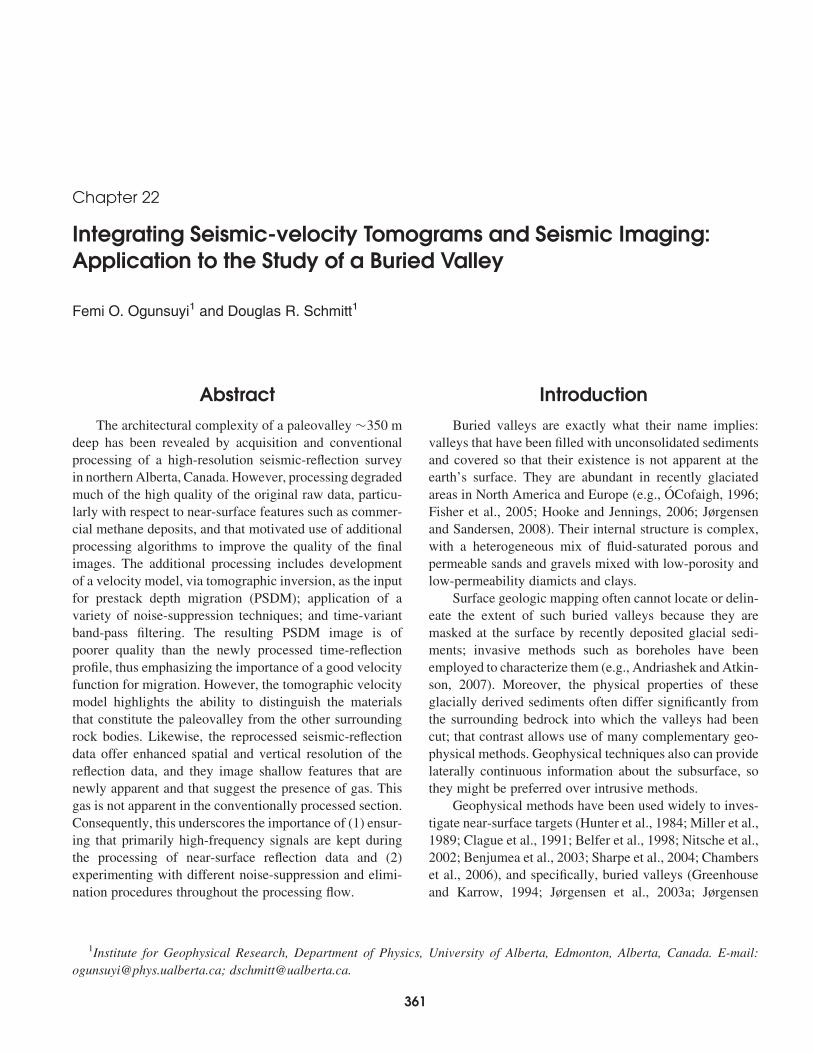
Download - Integrating Seismic-velocity Tomograms and Seismic Imaging

Chapter 22

Integrating Seismic-velocity Tomograms and Seismic Imaging:Application to the Study of a Buried Valley

Femi O. Ogunsuyi1 and Douglas R. Schmitt1

Abstract

The architectural complexity of a paleovalley �350 m

deep has been revealed by acquisition and conventional

processing of a high-resolution seismic-reflection survey

in northern Alberta, Canada. However, processing degraded

much of the high quality of the original raw data, particu-

larly with respect to near-surface features such as commer-

cial methane deposits, and that motivated use of additional

processing algorithms to improve the quality of the final

images. The additional processing includes development

of a velocity model, via tomographic inversion, as the input

for prestack depth migration (PSDM); application of a

variety of noise-suppression techniques; and time-variant

band-pass filtering. The resulting PSDM image is of

poorer quality than the newly processed time-reflection

profile, thus emphasizing the importance of a good velocity

function for migration. However, the tomographic velocity

model highlights the ability to distinguish the materials

that constitute the paleovalley from the other surrounding

rock bodies. Likewise, the reprocessed seismic-reflection

data offer enhanced spatial and vertical resolution of the

reflection data, and they image shallow features that are

newly apparent and that suggest the presence of gas. This

gas is not apparent in the conventionally processed section.

Consequently, this underscores the importance of (1) ensur-

ing that primarily high-frequency signals are kept during

the processing of near-surface reflection data and (2)

experimenting with different noise-suppression and elimi-

nation procedures throughout the processing flow.

Introduction

Buried valleys are exactly what their name implies:

valleys that have been filled with unconsolidated sediments

and covered so that their existence is not apparent at the

earth’s surface. They are abundant in recently glaciated

areas in North America and Europe (e.g., OCofaigh, 1996;

Fisher et al., 2005; Hooke and Jennings, 2006; Jørgensen

and Sandersen, 2008). Their internal structure is complex,

with a heterogeneous mix of fluid-saturated porous and

permeable sands and gravels mixed with low-porosity and

low-permeability diamicts and clays.

Surface geologic mapping often cannot locate or delin-

eate the extent of such buried valleys because they are

masked at the surface by recently deposited glacial sedi-

ments; invasive methods such as boreholes have been

employed to characterize them (e.g., Andriashek and Atkin-

son, 2007). Moreover, the physical properties of these

glacially derived sediments often differ significantly from

the surrounding bedrock into which the valleys had been

cut; that contrast allows use of many complementary geo-

physical methods. Geophysical techniques also can provide

laterally continuous information about the subsurface, so

they might be preferred over intrusive methods.

Geophysical methods have been used widely to inves-

tigate near-surface targets (Hunter et al., 1984; Miller et al.,

1989; Clague et al., 1991; Belfer et al., 1998; Nitsche et al.,

2002; Benjumea et al., 2003; Sharpe et al., 2004; Chambers

et al., 2006), and specifically, buried valleys (Greenhouse

and Karrow, 1994; Jørgensen et al., 2003a; Jørgensen

1Institute for Geophysical Research, Department of Physics, University of Alberta, Edmonton, Alberta, Canada. E-mail:

[email protected]; [email protected].

361

et al., 2003b; Steuer et al., 2009). In particular, refraction-

and reflection-seismic methods have been used extensively

in various glacial environments to image subsurface struc-

tures (e.g., Roberts et al., 1992; Wiederhold et al., 1998;

Buker et al., 2000; Juhlin et al., 2002; Schijns et al.,

2009) and to study buried valleys (Buker et al., 1998;

Francese et al., 2002; Fradelizio et al., 2008). In such

studies, seismic inversion often is limited to first-arrival

traveltimes for the input (e.g., Lennox and Carlson, 1967;

Deen and Gohl, 2002; Zelt et al., 2006), rather than input-

ting both refracted and reflected traveltimes (e.g., De Iaco

et al., 2003).

The fresh groundwater within buried valleys is usually

their most important resource. Consequently, in the last 15

years, numerous and varied geophysical investigations have

been undertaken in northern Europe (e.g., Gabriel et al.,

2003; Sandersen and Jørgensen, 2003; Wiederhold et al.,

2008; Auken et al., 2009) and North America (e.g.,

Sharpe et al., 2003; Pullan et al., 2004; Pugin et al., 2009)

to locate and define such features for their exploitation

and protection. Further, the porous sands and gravels in

buried valleys also can contain local biogenic gas (Pugin

et al., 2004) or leaked thermogenic methane. Such gas

sometimes exists in modest commercial quantities, but it

also can be a significant safety hazard for drillers.

Ahmad et al. (2009) recently described an integrated

geologic, well-log, direct-current electrical, and seismic-

reflection study of one such large buried valley in northern

Alberta, Canada. Using the same seismic data set, we

extend Ahmad et al.’s (2009) work by exploring develop-

ment of a seismic tomographic velocity model to character-

ize the paleovalley on the basis of the material/intervalvelocities. The model was generated by performing an

inversion of the traveltimes of both refracted and reflected

waves.

Refracted, guided, air, and surface waves are examples

of source-generated noise (coherent noise) that presents con-

siderable problems during seismic data processing (Buker

et al., 1998; Montagne and Vasconcelos, 2006). Accurate

separation of refracted and guided waves from shallow

reflections is difficult, and such linear events can stack

coherently on reflection profiles, causing misinterpretation

(Steeples and Miller, 1998). Performing a noise-cone

muting might prove useful in eliminating some of the

source-generated noise, but reflections also are muted in

the process (Baker et al., 1998). Surgical noise-cone

muting was employed to remove the coherent noise in the

previous study (Ahmad, 2006; Ahmad et al., 2009). Apart

from the possibility that this procedure might not have

removed the guided waves located outside the noise-cone

zone on the shot gathers, it inadvertently also might have

eliminated some true reflections during muting. Either way,

the resulting seismic profile is not as satisfactory as one

might expect from the quality of the raw shot gathers.

Therefore, in our study, we instead performed radial and

slant-stack noise-suppression procedures on the data set to

retain and enhance shallow reflections that might have been

removed by muting or masked by source-generated noise.

Because the dominant frequency of a seismicwave con-

trols the separation of two close events (Yilmaz, 2001), our

new processing scheme was aimed also at improving the

spatial and vertical resolution of the data set because the

seismic-processing sequence of the previous study did not

account for adequately filtering out the low frequencies.

We subsequently attempted to use the tomographic velocity

model to perform a prestack depth migration (PSDM) after

the noise-suppression strategies had been used on the data

set. To our knowledge, PSDM algorithms and the radial and

t-p noise-suppression techniques that often are employed in

more conventional and deeper petroleum exploration have

not been applied to such near-surface seismic data.

The goal here is not to provide a new geologic interpret-

ation of Ahmad et al.’s (2009) study, but instead to share

the experiences gained in applying several tools, some of

which to our knowledge have been employed heretofore

only in deeper petroleum exploration. One special improve-

ment over the earlier work is that this reprocessing has per-

mitted imaging of shallow methane deposits within the

glacial materials, and as such this work has implications

for both resource exploration and safety enhancement for

drillers.

Background

Details and maps of the location of the survey in the

northwestern corner of Alberta, centered at approximately

588 350 N and 1188 310 W, are found in Ahmad et al. (2009).

The near-surface geology of northeastern British Columbia

and northwestern Alberta has been studied extensively in

the last decade (e.g., Best et al., 2006; Hickin et al., 2008;

Levson, 2008). The surface geology of the area immedi-

ately over the profile has been investigated by Plouffe

et al. (2004) and Paulen et al. (2005), and it is established

to be blanketed primarily with glacial, lacustrine, and gla-

ciolacustrine sediments of variable depths; those authors

also have produced numerous complementary maps of the

region’s general surface geology.

A brief explanation of the bedrock geology is necessary

to assist the reader’s understanding of later geophysical

responses. The consolidated bedrock sediments beneath

Advances in Near-surface Seismology and Ground-penetrating Radar362

the Quaternary cover in the region lie nearly flat, and when

they are undisturbed they consist of �250 m of Cretaceous

siliclastic sands and shales underlain, across a sharp uncon-

formity (sub-Cretaceous), by more indurated Paleozoic

carbonates and shales. Hickin et al. (2008) and references

therein offer more detailed descriptions of the region’s

bedrock geology. Ahmad et al. (2009) also provide repre-

sentative well logs that, to first order, approximately cate-

gorize the sediments on the basis of sonic velocity and

density.

Seismic Field Program

A high-resolution 2D seismic profile was acquired over

a survey length of approximately 9.6 km in an east-west

direction (Figure 1). The seismic survey line straddles

the surface over the large buried valley to the east and the

out-of-valley region to the west, as determined from the

maps of bedrock topography and surface geology (Plouffe

et al., 2004; Paulen et al., 2005; Pawlowicz et al., 2005a,

2005b) (Figure 1). The purpose of the survey was to

image the formation above the sub-Cretaceous unconfor-

mity and hence to delineate the buried channel and obtain

important information about its internal structure.

A summary of the acquisition parameters is provided in

Table 1. The P-wave seismic source used was the Univer-

sity of Alberta’s IVI MinivibTM unit, operated with linear

sweeps of a 7-s period, from 20 Hz to 250 Hz, at a force

of approximately 26,690 N (6000 lb). The seismic traces

were acquired with high-frequency (40-Hz) geophone

singles (to attenuate some of the ground-roll noise) at a

4-m spacing using a 240-channel semidistributed seismo-

graph that consists of 10 24-channel GeodeTM field boxes

connected via field intranet cables to the recording compu-

ter. Approximately five to eight sweeps per shotpoint were

generated by the seismic source at a 24-m spacing. Cross-

correlation of the seismic traces with the sweep signal (to

generate a spike source), as well as vertical stacking, were

carried out in the field. The final stacked records were

saved in SEG2 format and later were combined with

survey header information into a single SEGY format file

for processing.

Generally, good coupling between the vibrator plate

and the frozen, snow-covered ground was achieved, as

determined by the constant nature of the force over time

during the sweep period and by the transmission of high

seismic frequencies (Ahmad et al., 2009). In a similar

manner, there was good coupling between the ground and

the geophones, which were frozen in place overnight, thus

improving the signal-to-noise ratio (S/N). The average

West

Contour interval = 25 m

200

200

300

9600

4800

100

0

400

km 10 0

6 0 miles

East

Figure 1. Contours of bedrock-topography elevation in

meters above sea level (asl), with the location of the 2D survey

line shown as a broken line. Black labels inside gray boxes

indicate distance in meters from east to west, with the origin at

0 m. The small unfilled circles are wellbore locations used to

generate the bedrock-topography map. After Pawlowicz et al.

(2005a). Used courtesy of Alberta Energy and Utilities Board/Alberta Geological Survey.

Table 1. Acquisition parameters for the 2D seismic survey.

Parameter Value

2D line direction East-west

Length of profile �9.6 km

Source 6000-lb IVI MinivibTM unit

Source frequency 20–250 Hz

Source type Linear

Source length 7 s

Source spacing 24 m

Vertical stacks 5–8

Number of unique shotpoints 399

Receivers 40-Hz single geophones

Receiver spacing 4 m

Recording instrument Geometrics GeodeTM system

Number of channels 192–240

Sampling interval 0.5 ms

Record length 1.19 s

Nominal fold �40

Chapter 22: Integrating Seismic-velocity Tomograms and Seismic Imaging 363

common-midpoint (CMP) fold for the survey was approxi-

mately 40. Two representative shot gathers from either end

of the seismic profile (Figure 2) highlight the evolution of

the traveltimes (and hence of velocity structure) from east

to west.

Seismic Traveltime Inversion

A linearized traveltime-inversion procedure, developed

primarily for modeling 2D crustal refraction andwide-angle

data (comprehensively described in Zelt and Smith, 1992;

and applied in Song and ten Brink, 2004), was used. The

inversion incorporates traveltimes of the direct, refracted,

and reflected events. The geometry of the model is outlined

by boundary node points that are connected through linear

interpolation, whereas the velocity field is specified by ve-

locity value points at the top and base of each layer. The ve-

locity within each block varies linearly with depth (between

the upper and lower velocities in a layer) and laterally

across the velocity points along the upper and lower layer

boundaries.

Examination of the refracted events on the shot gathers

offers an important insight into the apparent velocity struc-

ture of the survey line. Figure 2a shows a shot gather

acquired at the east end of the profile immediately over

the buried valley. Performing a simple intercept-time re-

fraction analysis on this gather suggests that a simple two-

layer model could be sufficient (see Ahmad et al., 2009).

The wave passage through the top layer (gray highlight)

might be linked to a lower material velocity of the Quater-

nary fill compared with the higher velocity of the Devonian

carbonates (yellow highlight). The velocity of the Quater-

nary rock is expected to be much lower than that of the

Paleozoic rocks because of its weak consolidation, which

resulted from minimal overburden pressures. On the other

hand, the shot gather obtained at the west end and outside

of the buried valley indicates three layers (Figure 2b):

(1) a direct wave (gray highlight) that passes through a

thin low-velocity Quaternary rock, (2) a refracted event,

of intermediate velocities, from the top of the Cretaceous

rock, and (3) another wave, with higher velocities, refracted

from the top of the Paleozoic.

The Vistaw processing package (GEDCO, Calgary)

was used to pick the traveltimes within the shot gathers of

both the refracted and reflected arrivals. Approximately

72,000 traveltime picks were made from 143 shot gathers,

and these were assigned an average error of+ 5 ms to

account for far-offset ranges and large depths (Ogunsuyi

et al., 2009). The program RayGUI (Song and ten Brink,

2004) was used for the forward modeling and inversion.

After a series of tests was conducted to determine

the optimal initial model, the starting model chosen was

constructed with six layers, with the velocities varying lin-

early in each layer. The starting model was made up of

coinciding locations of velocity and boundary nodes,

which were almost equally spaced laterally at a distance

of about 330 m for the top of the second and third layers,

and were spaced irregularly for the other layers. Short-

offset (,100-m) direct arrivals were inverted in the first

layer to account for the near-surface velocity variations

and the relatively flat surface topography. The second

layer was defined for the inversion of the rest of the direct

waves (the gray highlights in Figure 2), which constituted

the greater part of the seismic waves through the Quaternary

deposits. The third layer was defined for the refracted events

Figure 2. Raw shot gathers acquired at different locations on

the survey line. The apparent velocities of different refractors,

obtained from a simple intercept-time refraction method, are

displayed. Positive-offset values are to the west of the re-

spective shotpoint, whereas negative offsets are to the east.

The gray highlight shows a direct wave through the Quater-

nary fill, the blue highlight is a refracted wave turning through

the Cretaceous rock, the yellow line denotes the refracted

wave through the Devonian, and the reflection from the top of

the Devonian is in green. (a) An eastern shot gather (shotpoint

360) acquired over the valley on the seismic line. (b) A west-

ern shot record (shotpoint 1848) acquired outside the buried

valley.


turning through the Cretaceous rock (i.e., the blue highlight

in Figure 2b), whereas the base of the fourth layer rep-

resented the waves that reflected prominently from the

top of the sub-Cretaceous unconformity. Technically, the

third and fourth layers are supposed to be one and the

same, but they were separated to give a measure of the val-

idity of the final tomographic model, as demonstrated by the

degree to which the gap (in depth) between the base of the

third layer and base of the fourth layer will be reduced sub-

sequent to the inversion process. The refracted events

(yellow highlights in Figure 2) through the Devonian rock

were inverted for the fifth layer. A reflected event that

could not be picked successfully for the whole length of

the survey line was inverted for layer six, so less confidence

is placed on the tomographic results at elevations below

�200 m below sea level.

The model was inverted layer by layer, from the top

down, in a layer-stripping method intended to speed up

and simplify the process (Zelt and Smith, 1992). This

method involved the following steps: (1) simultaneously

inverting the model parameters (both velocity and boundary

nodes) of the topmost layer, (2) updating the model with

the calculated changes, (3) repeating steps 1 and 2 until

the stopping criteria are satisfied for the layer, (4) holding

the model parameters of the layer constant for the sub-

sequent inversion of all the parameters of the next layer in

line, and (5) repeating steps 1 through 4 for all the other

underlying layers in sequence. The uncertainties in the

depths of the boundary nodes and velocity values were

10 m and 200 m/s, respectively.The average values for the root-mean-square (rms)

traveltime residual between the calculated and observed

times for all layers was 16.4 ms after seven iterations.

Notably, adding more model parameters generally reduces

the traveltime residual, but it does so at the expense of re-

ducing the spatial resolution of the final model parameters

(Zelt and Smith, 1992). Subsequent to the inversion, the

difference in depth between the bases of the third and

fourth layers was reduced acceptably on the west but was

not reduced adequately on the east end inside the valley

area.Merging the third and fourth layers before the inversion

scheme, however, produced low ray coverage, thus violating

one of the conditions for choosing a final model. Conse-

quently, the six-layer model was chosen as the optimal

model for the subsurface of the area under investigation.

Processing of Seismic-reflection Data

Ahmad et al.’s (2009) earlier study involves a conven-

tional 2D CMP processing scheme (Table 2) whereas the

new processing sequence (adapted from Spitzer et al.,

2003) followed in this study is complemented with noise-

suppression procedures that involve transformation of

time-space (t-x) data into other domains (Table 3). The

motivation for designing a new processing scheme for the

seismic data was the need to determine whether reflections

were eliminated or degraded by the muting functions

adapted in the previous study or were covered up by

source-generated noise. If either was the case, we wished to

recover the affected reflections and additionally to improve

the lateral and vertical resolutions of the reflection profile.

Low-quality traces resulting from noisy channels, high

amplitude, and frequency spikes are problematic to a final

image. Starting with the data set that already has geometry

information assigned, the bad traces, with abnormally high

amplitudes and frequencies, were identified by computing

amplitude and frequency statistics on all the traces and

Table 2. Previous seismic processing sequence, as performed

by Ahmad et al. (2009).

Processing step Parameters

Geometry —

Editing of bad trace —

Offset limited sorting –500 m to –12 m and

12 m to 500 m

Surgical mute Auto bottom mute;

manual surgical mute

CMP sorting 4-m bin size

Velocity analyses —

NMO corrections 15% stretch mute

Elevation/refraction statics

corrections

400-m asl datum; 1500 m/sreplacement velocity

Residual statics corrections Stack power algorithm

Inverse NMO corrections —

Final velocity analyses —

NMO corrections 15% stretch mute

Final residual statics

corrections

Stack power algorithm

CMP stack —

Band-pass filtering 45 to 240 Hz

Mean scaling —

f-x prediction —

Automatic gain control 150 ms


subsequently were removed. To adjust for the lateral chang-

es in the thickness and velocity of the shallow depths and

for the small elevation variations of sources and receivers,

elevation/refraction statics corrections were conducted. A

model of the shallow subsurface was established by in-

verting the first-break picks. Using a weathering velocity

of 500 m/s, the average velocity of the first refractor was

approximately 1700 m/s. The computed statics corrections

were applied to a flat datum of 385 m above sea level, which

was slightly above the highest elevation of the survey line.

Total elevation/refraction statics corrections ranged from

approximately –6.5 ms to þ21 ms.

Predictive deconvolution was not successful in remov-

ing some of the multiples in the data at this stage, so it was

carried out in later processing. To compress the wavelet to

a spike and thereby to increase the temporal resolution,

spiking deconvolution was applied. After testing with

different operator lengths for optimal results, a 20-ms oper-

ator length finally was employed. Low frequencies in the

amplitude spectrum of the seismic data were dominated

by direct and surface waves, but application of a low-cut

frequency filter to the data set for the purpose of suppressing

the noise might also inadvertently remove some deeper

reflections that are characterized by low frequencies. To

avoid this, time-variant band-pass filtering was applied to

the data (80–300 Hz for a 0- to 380-ms time interval and

65–150 Hz for a 380- to 800-ms interval).

In addition, the band-pass-filtering step provides a

means of enhancing temporal resolution of the seismic

profile. Following the spiking deconvolution step, the

amplitude spectra of the shot gathers were equalized ade-

quately. To appreciate the value of these processing steps,

a raw shot gather (shot-point number 660), affected by

surface waves after elevation/refraction statics corrections

(Figure 3a) and after application of spiking deconvolution,

band-pass filtering, and trace equalization (Figure 3b), is

displayed for comparison. Although most of the source-

generated noise has not been eliminated, most of the

surface waves have been suppressed and the reflection

wavelet improved. Moreover, this processing step appears

to have exposed additional guided waves that were con-

cealed in the initial shot gather (Figure 3b). Details about

the properties of these common seismic arrivals, which

form the basis of our interpretation, can be found in

Robertsson et al. (1996) and in Yilmaz (2001).

Choosing the best possible CMP bin size is imperative

for minimizing spatial aliasing when one is processing

seismic data for moderately to steeply dipping reflections

(Spitzer et al., 2003). To determine the maximum CMP

bin size b to use (Yilmaz, 2001), we evaluated

b Vmin

4fmaxsinu; (1)

where Vmin is the minimum velocity, fmax is the maximum

frequency, and u is the maximum expected dip of structures.

We arrived at a value of 3 m as the appropriate bin size for

our data. Initial velocity analyses to determine the stacking

Table 3. Time-processing sequence for the 2D seismic

survey.

Processing step Justification

Trace editing Removal of spurious traces

First-break picking

Elevation/refraction statics

corrections

Correction for shallow lateral

variations

Spiking deconvolution Compression of wavelet

Time-variant band-pass

filtering

Suppression of low-

frequency noise

Trace equalization

CMP binning

Initial velocity analyses Determination of stacking

velocities

NMO corrections

Residual statics corrections Correction for near-surface

velocity changes

Inverse NMO corrections

Radial domain processing Removal of guided waves

Linear t-p processing Suppression of source-

generated noise

Predictive deconvolution Elimination of multiples

Dip-moveout (DMO)

corrections

Preservation of conflicting

dips

Final velocity analyses Determination of stacking

velocities

Final residual statics

corrections

Correction for near-surface

velocity changes

NMO corrections

CMP stack

f-x prediction Reduction of incoherent

noise

2D Kirchhoff time migration Placing reflections in their

true positions


velocities were carried out on CMP supergathers by creat-

ing a panel of offset sort/stack records, constant-velocity

stacks, and semblance output.

Residual statics are needed to correct for short-wave-

length changes in the shallow velocity underneath each

source-and-receiver pair. Surface-consistent residual statics

by a stack power-maximization algorithm (Ronen and

Claerbout, 1985) were estimated from the data after apply-

ing normal-moveout (NMO) corrections on the basis of the

initial velocity analyses. The resulting average time shifts

80

100

a) b)

c) d)

e) f)

g) h)

200

300 Tim

e (m

s)

400

100

200

300 Tim

e (m

s)

400

100

200

300 Tim

e (m

s)

400

100

200

300 Tim

e (m

s)

400

Surface waves

Guided waves

160 240 320 Source-receiver offset (m)

400 480 560 80 160 240 320 Source-receiver offset (m)

Apparent velocity (m/s)

400 480 560

100

200

300

t′ =

t +

30

– (x

⁄ 18

80)

(ms)

400

100

200

300 Tim

e (m

s)

400

100

200

300 Tim

e (m

s)

400

100

200

300

τ (m

s)

400

Guided waves

Remnants of guided waves

Guided waves

Pass region of filter

80 160 240 320 Source-receiver offset (m)

400 480 560


400 480 560


400 480 560

–0.8 –0.6 –0.4 –0.2 Slowness (ms/m)

0.0 0.2 0.4

2500200015001000500Apparent velocity (m/s)

2500200015001000500

Figure 3. (a) A typical raw shot gather

(shotpoint number 660) after elevation/refraction static corrections. (b) The same

shot gather as in (a), after spiking decon-

volution, time-variant band-pass filtering,

and trace equalization. (c) The same shot

gather as in (b), but after transformation to the

r-t domain. (d) The same shot gather as in (c),

after applying a low-cut filter of 45 Hz to

suppress the linear events. (e) The same shot

gather as in (d), after radial processing that

involved transforming the shot gather from

r-t to t-x coordinates. (f) The same shot gather

as in (e), except that the time axis is reduced:

traveltimes t0 ¼ tþ 30 – (x/1880), where1880 m/s is the average velocity for the first

arrival (as obtained from intercept-time

refraction analyses). (g) The same shot gather

as in (f), after linear t-p transformation. The

pass region of the t-p filter is shown by a solidblack line. (h) Result of linear t-p processingobtained from filtering (g) and applying the

inverse t-p transformation. The records were

scaled in relation to the rms amplitude of their

respective gathers.


of about 4 ms were applied subsequently to the inverse

NMO-corrected data.

As was noted earlier, most of the source-generated

noise was not eliminated by band-pass filtering. Linear

events (e.g., guided waves), which can affect the interpre-

tation of shallow seismic adversely if they are not sup-

pressed, still can be observed (Figure 3b). Some of this

coherent noise can be reduced by mapping the data from

a normal t-x domain into an apparent-velocity versus

two-way-traveltime (radial or r-t) domain. The basis of

this noise-attenuation process is that linear events in the

t-x gather transform into a relatively few radial traces,

with apparent frequencies shifting from the seismic band

to subseismic frequencies (Henley, 1999). After transform-

ation to the r-t domain (Figure 3c), a low-cut filter of 45 Hz

was applied to the radial traces (Figure 3d) to eliminate the

coherent noise mapped by an r-t transform to low frequen-

cies. Subsequently, the data were transformed back to the

t-x domain (Figure 3e). With regard to removal of some

of the guided waves, the improvement of the data passed

through radial processing (Figure 3e) compared with the

quality of the original (Figure 3b) is quite noticeable.

To further reduce the source-generated noise (direct

waves, surface waves, and remnants of guided waves) in

the data, linear time-slowness (t-p) processing was

applied next. Linear and hyperbolic events in the t-x

domain are mapped into points and ellipses, respectively,

in the linear t-p (or slant-slack) domain during linear t-ptransformation (Yilmaz, 2001). Hence, it is possible to sep-

arate these events in slant-slack gathers, to facilitate noise

suppression. The steps involved in the linear t-p processingare outlined below (modified from Spitzer et al., 2001).

1) The shot gathers were converted to reduced-traveltime

format (linear-moveout terms) using velocities derived

from intercept-time refraction analyses. To generate

the gathers,

t0 ¼ t þ 30� (x=Vav) (2)

was applied to each trace, where t0 is the reduced time in

milliseconds, t is the original time in milliseconds, x is

the source-receiver offset in meters, and Vav is the

average velocity in kilometers per second. Generally,

the average velocities change across the survey line.

A bulk shift of 30 ms was applied to the data to accom-

modate possible overcorrections of linear moveout. As

seen in Figure 3f, the first arrivals and related source-

generated noise have been converted to horizontal or

nearly horizontal events.

2) Because the recording direction is not preserved during

t-p mapping (Spitzer et al., 2001), we separated the

positive source-receiver offsets from negative offsets

before processing them further.

3) The reduced-traveltime shot gathers were transformed

into the linear t-p domain using a range of p (slowness)

values from –0.9 to 0.4 ms/m for positive offsets and

–0.4 to 0.9 ms/m for negative offsets, to exclude

surface waves and other low-velocity coherent noise,

and with t being intercept time. Although minor alias-

ing of the surface waves was observed in the

slant-stack gathers (as observed in the frequency-wave-

number or f-k domain) of the data, it does not seem to

pose a major problem to our data.

4) The reflected events (i.e., ellipses) in the t-p domain are

quite distinguishable from the source-generated noise

(mapped to points around p ¼ 0 ms/m). We defined a

2D pass filter (as illustrated in Figure 3g) around the

elliptical events for data on each side of the split

source-receiver offset, and we set the amplitudes of

the regions outside the area to zero. A 5-ms taper was

applied in the t direction to the data, to minimize

artifacts.

5) We then performed inverse linear t-p transformation

on the filtered t-p data. Subsequently, the data for the

positive and negative offsets were recombined, and

the linear moveout terms and the time bulk shift were

removed. The results show that most of the linear

source-generated noise has been reduced with no

adverse effect on the reflections (Figure 3h).

Some linear events still remain in the data. This could

be because spatially aliased events in the t-x domain might

spread over a range of slowness values, including the pass

region of the filter, in the t-p domain (Spitzer et al.,

2001). These remnant linear events were removed carefully

by surgical muting. Applying predictive deconvolution

with 150-ms operator length and a prediction distance of

15 ms at this stage appeared to remove some of the mul-

tiples at greater depths.

Stacking velocities are dip-dependent, so in the case of

an intersection between a flat event and a dipping event, one

can choose a stacking velocity in favor of only one of these

events, not both (Yilmaz, 2001). Dip-moveout (DMO) cor-

rection preserves differing dips with dissimilar stacking vel-

ocities during stacking. We applied DMO corrections to the

NMO-corrected gathers (using velocities from the initial

conventional CMP velocity analyses) and then performed

an inverse NMO on the resultant data. Subsequently, a

final velocity analysis was carried out on CMP supergathers

(made up of 15 adjacent composite CMPs). The stacking

velocities of the t-p-processed and DMO-corrected data

can be picked with greater assurance compared with the


data that were not passed through those processing steps.

The final stacking velocities from conventional CMP ve-

locity analyses (Figure 4a) and the corresponding interval

velocities after conversion (Figure 4b) show the lateral

variation in the velocities from the buried valley to the

Cretaceous bedrock, as does the result of the tomographic

inversion (Figure 4c).

Using statics estimates that were computed after NMO

corrections based on the final stacking velocities had been

done, residual statics again were carried out. As a result

of NMO correction, a frequency distortion occurs, particu-

larly for shallow events and large offsets (Yilmaz, 2001). A

stretch mute of 60% was applied to the data to get around

that problem. The data later were stacked and frequency-

space ( f-x) prediction was performed on the data to

reduce incoherent noise (Canales, 1984). For display pur-

poses, an automatic gain control of 300 ms was applied to

the final stacked section (Figure 5a). To place the reflections

in the true subsurface positions, 2D Kirchhoff poststack

time migration also was performed on the seismic data

(Figure 5b).

Although it is possible to make an interpretation about

the structure of the buried valley from the time-stack sec-

tion, correlation with depth values cannot be made without

having a time-depth relationship. We conducted a simple

depth conversion of the seismic section, using average ve-

locities from the generated tomographic model and from

conventional CMP velocity analyses. However, the results

showed a prominent reflection (the sub-Cretaceous uncon-

formity) being pulled down substantially at the west end

of the profile. This probably is the result of the consider-

able lateral variation in velocity. Instead, prestack depth-

migration (PSDM) processing was performed on the data,

after the noise-suppression procedures (as outlined in

Table 4), by using the velocity distribution derived from

the traveltime tomography of refracted and reflected events

Figure 4. (a) Final stacking velocities as

picked during traditional velocity analyses

on CMP supergathers. The vertical axis

is two-way time in milliseconds. (b) for the

same data as in (a), after conversion to

interval velocities. (c) The interval

velocities of the subsurface, as acquired

from the traveltime inversion with a

vertical exaggeration of about five. The

vertical axis is elevation (m) above sea

level (asl). The different rock bodies, as

labeled, can be distinguished on the basis

of their respective material velocities.


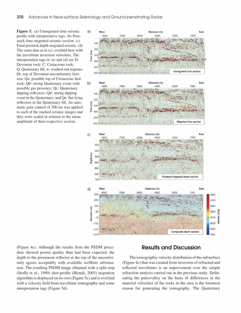
(Figure 4c). Although the results from the PSDM proce-

dure showed poorer quality than had been expected, the

depth to the prominent reflector at the top of the unconfor-

mity agrees acceptably with available wellbore informa-

tion. The resulting PSDM image obtained with a split-step

(Stoffa et al., 1990) shot-profile (Biondi, 2003) migration

algorithm is displayed on its own (Figure 5c) and is overlaid

with a velocity field from traveltime tomography and some

interpretation tags (Figure 5d).

Results and Discussion

The tomographic velocity distribution of the subsurface

(Figure 4c) that was created from inversion of refracted and

reflected traveltimes is an improvement over the simple

refraction analysis carried out in the previous study. Delin-

eating the paleovalley on the basis of differences in the

material velocities of the rocks in the area is the foremost

reason for generating the tomography. The Quaternary

Figure 5. (a) Unmigrated time seismic

profile with interpretative tags. (b) Post-

stack time-migrated seismic section. (c)

Final prestack depth-migrated seismic. (d)

The same data as in (c), overlaid here with

the traveltime inversion velocities. The

interpretation tags in (a) and (d) are D:

Devonian rock; C: Cretaceous rock;

Q: Quaternary fill; w: washed-out regions;

Dt: top of Devonian unconformity hori-

zon; Qa: possible top of Cretaceous bed-

rock; Qb: strong Quaternary event with

possible gas presence; Qc: Quaternary

dipping reflectors; Qd: strong dipping

event in the Quaternary; and Qe: flat-lying

reflectors in the Quaternary fill. An auto-

matic gain control of 300 ms was applied

to each of the stacked seismic images and

they were scaled in relation to the mean

amplitude of their respective section.


sediments in the east are distinguished readily from the Cre-

taceous bedrock in the west with material velocities, which

vary from�1700 m/s in the buried valley to�2800 m/s inthe bedrock (Figure 4c). This is not surprising because the

Quaternary-fill deposits are expected to be loosely consoli-

dated (thereby giving rise to lower compressional-wave

velocities) compared with the stiffer Cretaceous bedrock.

Accordingly, the edge of the valley is defined by rapid

changes in the material velocities, as can be observed in

the inversion result at distances between 4800 and

6000 m. Vertically, the transition in the velocities from

the inversion (Figure 4c) is not abrupt, but the geologically

sharp unconformity (see Ahmad et al., 2009) at the base of

both the Cretaceous and Quaternary sediments still is

noticeable. The velocities rise rapidly in the tomographic

result to values .3500 m/s, which is typical of the deeper

Devonian carbonates. The stacking velocities that were

converted to interval velocities (Figure 4b) are comparable

to the final material velocities derived from the results of the

traveltime inversion (Figure 4c). The similarities, both in

magnitude and features, between the two velocity images

(Figure 4b and 4c) are apparent.

However, it is noteworthy that the edge of the valley (at

an approximate distance of 5700 m), as deduced from the

interval velocities (Figure 4b) derived from the picked

stacking velocities, appears more abrupt than is observed

in the tomographic velocity model (Figure 4c). This differ-

ence in velocity transition from the valley to the Cretaceous

rock could be related to challenges encountered in the

course of picking the stacking velocities on washed-out

CMP supergathers, because reflections were difficult to

detect in the washout zones.

It also is observed that the top of the sub-Cretaceous

unconformity (Ahmad et al., 2009), which is characterized

by a noticeable jump in velocities, appears to be more

uneven in the converted velocities (Figure 4b) than in the

results of the traveltime inversion (Figure 4c). Minor

errors in the stacking-velocity picking could account for

that contrast. It is clear that the tomographic data are suc-

cessful in delineating the paleovalley.

However, the low-resolution inversion results (Figure4c)

could not image details of the structure within the valley

that are evident in the reflection profiles (Figure 5a

and 5b). Some of the features include a variety of dipping

reflectors Qc at the edge of the valley; a strong, dipping

reflector Qd that is unconformable with the other reflectors;

and the numerous flat-lying reflectors Qe. Nonetheless,

because of inadequate well information within the valley

area, we cannot ascertain whether substantial material-

velocity differences exist in the various sediments that

constitute the buried valley. Further, if there are material-

velocity differences, we are not sure whether they can be

observed clearly on sonic logs.

To convert the time section to depth, we used the tomo-

graphic velocity model to perform a PSDM on the data

(Figure 5c and 5d). The quality of the results, however,

was not as good as anticipated, as can be observed from

the degraded reflection continuities, mostly in the western

part of the line (i.e., distances . 5000 m). This could be

related to minor problems in the velocity model, which

for improved results might require iterative refinement

with the aim of serving as input to the PSDM algorithm

(see Bradford and Sawyer, 2002; Morozov and Levander,

2002; Bradford et al., 2006). Seismic anisotropy also

might play a role here because the tomographic image,

which includes refracted head and turning waves, could

be biased by these more horizontal propagation paths. In

addition, because a 2D migration can only collapse the

Fresnel zone in the migration direction (Liner, 2004), the

discontinuous nature of the reflections in the PSDM data

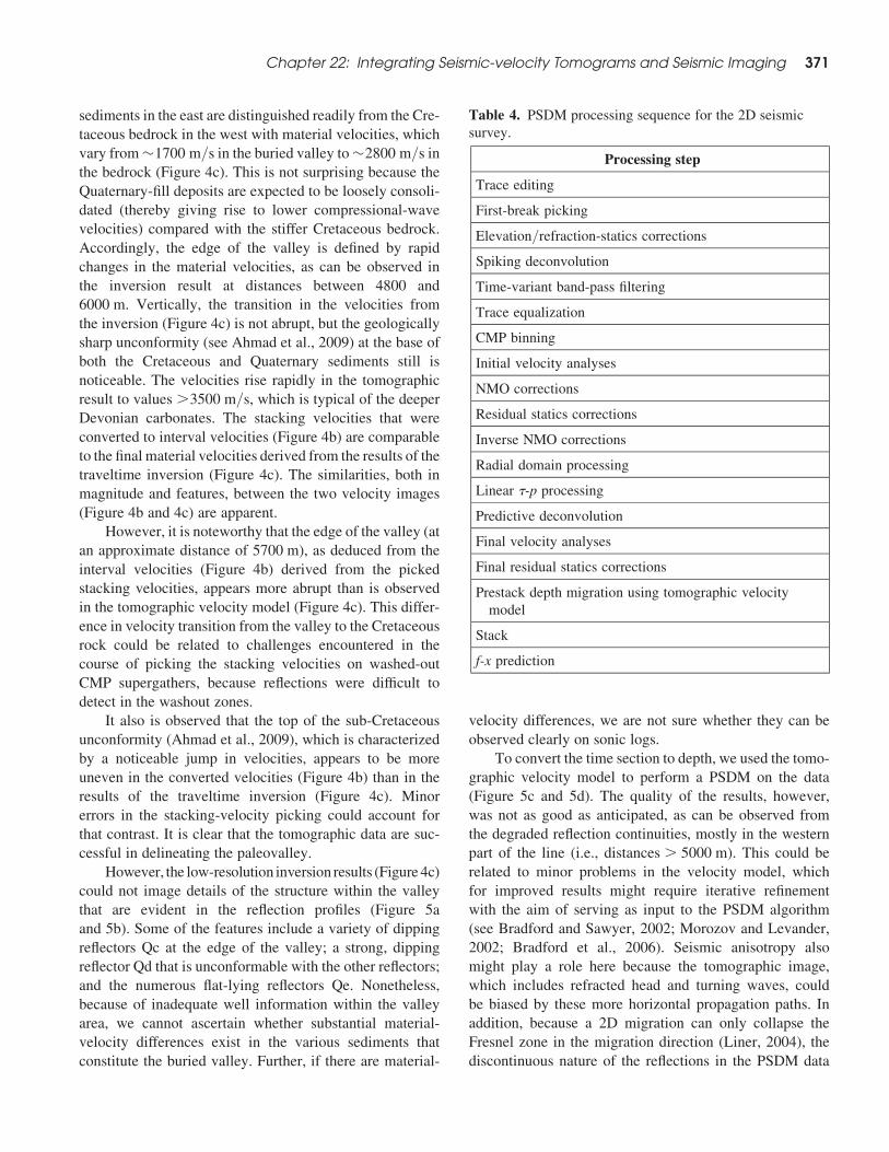
Table 4. PSDM processing sequence for the 2D seismic

survey.

Processing step

Trace editing

First-break picking

Elevation/refraction-statics corrections

Spiking deconvolution

Time-variant band-pass filtering

Trace equalization

CMP binning

Initial velocity analyses

NMO corrections

Residual statics corrections

Inverse NMO corrections

Radial domain processing

Linear t-p processing

Predictive deconvolution

Final velocity analyses

Final residual statics corrections

Prestack depth migration using tomographic velocity

model

Stack

f-x prediction


could result from the fact that we are imaging an irregular

3D structure into the 2D profile.

Most of the wellbores in the immediate vicinity of the

2D line are for shallow gas production; hence, they are

not deep enough to reach the top of the unconformity. None-

theless, two wells to the south at a distance of,3 km from

the survey line penetrated the unconformity at an elevation

of about 28 m above sea level, which is approximately 7 m

deeper than the depth to the unconformity that is clearly

observable on the PSDM image (Figure 5d). Considering

the uneven topography on top of the unconformity (Fig-

ure 5a), this minor discrepancy in depth is not unreasonable.

However, uncertainty is involved in estimating the top of

the unconformity — which is known from core and well

logs to be abrupt — using the “smeared” results of the

traveltime inversion. As mentioned earlier, the initially sep-

arated third and fourth layers of the tomographic velocity

model are supposed to be one and the same. However, sub-

sequent to the inversion they were merged adequately only

for the western part of the profile line and not for the eastern

side (i.e., for the distance of 1200 to 5100 m, see the section

on seismic traveltime inversion). Hence, either the top or

the base of the fourth layer can be picked as the top of the

unconformity. If the top of layer four is selected as the

top of the unconformity, the results of the traveltime inver-

sion and the PSDM stacked section agree, but if the base of

layer four is picked, a depth discrepancy of approximately

43 m occurs. In addition, estimating the depth of the uncon-

formity from the tomography, on the basis of an interpret-

ation of the colors, is quite subjective and easily biased.

The result of the reflection data processed previously

using conventional steps (without radial and linear t-p pro-cessing) (Ahmad et al., 2009) is displayed in Figure 6a, and

the result from the processing steps presented in this con-

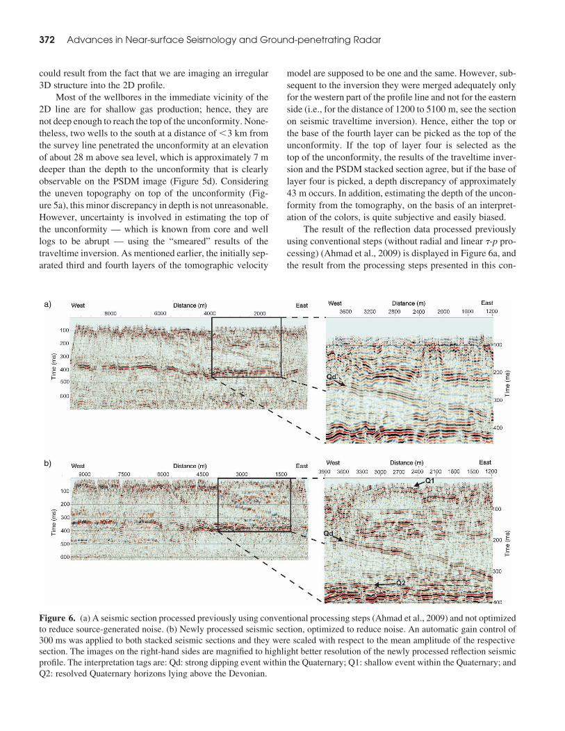
Figure 6. (a) A seismic section processed previously using conventional processing steps (Ahmad et al., 2009) and not optimized

to reduce source-generated noise. (b) Newly processed seismic section, optimized to reduce noise. An automatic gain control of

300 ms was applied to both stacked seismic sections and they were scaled with respect to the mean amplitude of the respective

section. The images on the right-hand sides are magnified to highlight better resolution of the newly processed reflection seismic

profile. The interpretation tags are: Qd: strong dipping event within the Quaternary; Q1: shallow event within the Quaternary; and

Q2: resolved Quaternary horizons lying above the Devonian.


tribution is shown in Figure 6b for comparison. In the

magnified images beside each profile, better temporal and

lateral resolution in the newly processed seismic is

observed. Using the quarter-wavelength limit of vertical

resolution (Widess, 1973) and a velocity of 2000 m/s, avertical resolution of 16.6 to 6.25 m was obtained for the

previously processed seismic data, from dominant frequen-

cies typically ranging from 30–80 Hz.

Similarly, a vertical resolution of 10 to 3.3 m was ob-

tained for the newly processed seismic profile, from domi-

nant frequencies primarily in the 50- to 150-Hz range. Eval-

uating the equation for the threshold of lateral resolution—

i.e., for the radius of the first Fresnel zone (Sheriff, 1980)—

with 1000 m/s as velocity at 150-ms two-way traveltime,

the lateral resolution of the seismic section from the pre-

vious study ranged from 35.4 to 21.6 m (30- to 80-Hz domi-

nant frequencies). That of the new seismic profile ranged

from 27.4 to 15.8 m (50- to 150-Hz dominant frequencies)

at about the same two-way traveltime. Thus, it is evident

from these values that the resolution of the data has been

enhanced in the new seismic profile.

It is unclear from the previous seismic profile (Fig-

ure 6a) whether the low-amplitude horizons immediately

below strong, dipping event Qd are flat lying or at an in-

cline. On the other hand, the new profile (Figure 6b) shows

clearly that the above-mentioned horizons dip from west

to east. Clarification of the dipping nature of these events

was perhaps a result of the improved resolution of the new

data, but one cannot rule out the possibility that the new pro-

cessing scheme recovered some eliminated parts of the re-

flections. Those parts could have been removed by the mute

functions used in the previous processing, thus making them

less coherent. At the distance of about 2400 to 3000 m and

the time 30 ms, it also is possible to identify a nearly hori-

zontal feature Q1 on the new seismic data (Figure 6b).

To avoid misinterpreting as reflections what really are

coherent events and artifacts from various processing

steps for enhancement (e.g., Steeples and Miller, 1990;

Steeples et al., 1997; Sloan et al., 2008), we attempted to

validate the true nature of the Q1 feature directly from the

filtered shot records (Figure 7a). However, this shallow

feature exhibited a lower frequency than did deeper reflec-

tions on shot gathers, and it could not be correlated with cer-

tainty to any true reflection. Thus, without additional

supporting evidence, the Q1 feature cannot be considered

to be any more than a stacked coherent event.

Clearly noticeable on the new seismic profile

(Figure 6b), between distances 3000 and 4200 m, are hori-

zons Q2, lying directly on top of the unconformity. On the

old seismic section (Figure 6a), these horizons appear to be

merged with the sub-Cretaceous unconformity and cannot

be distinguished easily. On the new profile, these high-

amplitude reflections seem to cover almost the entire

extent of the bottom of the valley, from distance 4200 m

on the west to distance 1200 m on the east — at which

point they become incoherent because of the smeared

zone. Considering the fact that these flat-lying reflectors

were not observed outside the paleovalley (distances

.6000 m), they are likely Quaternary sediments that were

deposited immediately after the erosion caused by glacial

meltwaters; alternatively, they might be remnants of the

erosion of the valley itself.

Washout/smeared zones were problematic to the

imaging (Figure 5). In particular, the western edge of the

40

50

100

Tim

e (m

s)

150

200

50

100

Tim

e (m

s)

150

200

120

Possible artifact

Gas reflection

Source-receiver offset (m)

–200 –120 –40

200

Source-receiver offset (m)a)

b)

Figure 7. Raw shot gathers after elevation/refraction static

corrections, spiking deconvolution, time-variant band-pass

filtering, and trace equalization, located near (a) the poorly

constrained shallow, 30-ms Q1 feature from Figure 6b, and

(b) a strong reflection that is interpreted to be the top of a

near-surface methane-saturated sand shown in Figure 8b.


valley (at approximately distance 5700 m) was not well

imaged because of a large washout zone at that location.

The washout zones are attenuated regions where continuous

reflections are not observed. As can be seen from the unpro-

cessed shot gathers, it is not possible to make out any strong

reflections in these zones. Although the exact cause of this

attenuation is not known, it likely is associated with thicker

zones of muskeg (bogs filled with sphagnum moss). The

most conspicuous event in the reflection sections is the

strong reflector Dt located approximately halfway down

the vertical axis of the profiles. Aside from the washout

zones W, this reflector, which is the unconformity above

the Devonian rock, spans the entire survey line. Above

the unconformity lie Cretaceous bedrock C to the west of

distance 6000 m and Quaternary sediments Q to the east

of distance 4800 m. The edge of the paleovalley, dipping

from west to east, lies between distances 4800 and 6000 m.

There is a shallow high-amplitude reflection Qa from

approximately distance 6000 to 9300 m at a two-way travel-

time of �50 ms (Figure 5a). This event could be the top of

the Cretaceous bedrock. It is interesting to note that the

reflection is not continuous across the entire survey line to

the valley area on the eastern side. A possible explanation

for this could be the minimal impedance contrast between

the glacial sediment that blankets the whole area and the

deposits that constitute the buried valley. This event could

not be seen clearly on the previously processed seismic

profile, which points to the fact that the new data are

improved relative to the old.

Shallow features that were not apparent in Ahmad

et al.’s (2009) previous processing (Figure 8a) now are

visible in Figure 8b and are particularly noteworthy. As

also can be seen on the PSDM seismic profile (Figure 5d),

there is a strong reflector Qb at an elevation of approxi-

mately 345 m above sea level (at an �40-m depth), inside

but at the edge of the valley (between distances 3900 and

5100 m). This strong reflector, also clearly visible in the

raw shot gathers (e.g., Figure 7b), likely indicates the pres-

ence of free gas. Such gas has been produced in commercial

quantities from this site (Rainbow and Sousa fields in

northern Alberta) in the last decade, at depths of less than

100 m (see Pawlowicz et al., 2004; Kellett, 2007), and it

still is being produced. Considering that the shallow gas

in the Rainbow field has a chemical signature that indicates

a deeper, thermogenic origin and given the high electrical

resistivities recorded in our survey area, it has been sug-

gested that gases migrated from the Cretaceous bedrock

formations and were trapped in the porous Quaternary sedi-

ments (Ahmad et al., 2009).

These shallow gas deposits had been found serendipi-

tously during previous drilling of shallow water or deeper

petroleum boreholes, and on numerous occasions they have

led to dangerous releases of flammable methane gas that

sometimes have destroyed rigs. Ground-based electrical-

resistivity tomography (ERT) studies have been used in

the past to indicate free, dry gas on the basis of high electri-

cal resistivities. However, separating gas-saturated zones

from freshwater-saturated zones can be difficult. The

result of reprocessing this current data set suggests that

with sufficient care, such shallow gas-filled zones can be

distinguished. Conducting high-resolution seismic surveys

over areas already targeted for drilling on the basis of

ERT could add confidence and warn drillers about potential

shallow blowout hazards.

Conclusions

We have presented the results of reanalyses of a near-

surface seismic data set acquired over a paleovalley in

northern Alberta, Canada. Our study includes (1) generation

of a traveltime inversion to better delineate the buried

valley, (2) reprocessing of the reflection data to enhance

their resolution and recover any muted or degraded ho-

rizon from the previous processing, and (3) employment

5600

a)

b)

0

100

200

4800 4000

Distance (m)

3900450051005700

Distance (m)

Gas bright spot

Tim

e (m

s)

0

100

200

Tim

e (m

s)

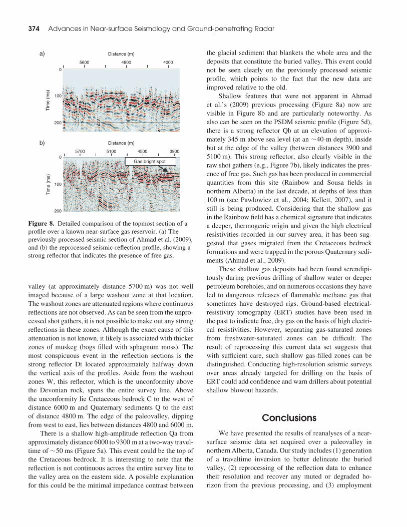
Figure 8. Detailed comparison of the topmost section of a

profile over a known near-surface gas reservoir. (a) The

previously processed seismic section of Ahmad et al. (2009),

and (b) the reprocessed seismic-reflection profile, showing a

strong reflector that indicates the presence of free gas.


of prestack depth migration, using velocities generated

from the traveltime inversion, to obtain proper presentation

of the data in depth scale.

Construction of tomographic velocity from inversion of

direct, refracted, and reflected waves aimed to determine

accurate representation of the velocity distribution of the

area over the buried valley. That accomplishment would

be an improvement over the results of the simple refraction

analysis performed in the previous study. The results from

the traveltime inversion show clearly that on the basis of

the material velocities, a buried valley can be delineated

from the surrounding rock bodies. The interval velocity of

the loosely consolidatedQuaternary-fill valleywas observed

to be approximately 1700 m/s, whereas that of themore com-

petent Cretaceous bedrock was approximately 2800 m/s;the edge of the valley was defined by rapid changes in the

material velocities. The interpretation made from the tomo-

graphic model is important because of the significant

knowledge it provides about velocity contrasts of different

materials. On the other hand, such detailed information

about exact contrasts in the physical properties that produce

reflections might not be deduced readily from seismic-

reflection profiles alone, particularly given the absence of

appropriate sonic and density well logs in the area. It is

noteworthy, however, that the resolution of the traveltime

inversion was insufficient to image the different rock fea-

tures within the valley clearly, perhaps because of the

structural complexities of the valley. It is suggested that

waveform inversion with the tomographic results as the

input model might be a viable option in imaging a paleoval-

ley with complex architecture.

The seismic-reflection data were processed with a strat-

egy optimized to enhance the lateral and vertical resolutions

of the profile. An additional goal was to recover any muted

or degraded reflection from the old study by employing

noise-suppression techniques in other domains as opposed

to the total muting of the noise cone in t-x coordinates.

The processing steps included radial and linear t-p proces-

sing used to reduce noise, and time-variant band-pass filter-

ing to improve resolution.

Better resolution and more continuous events charac-

terize the final stack of the newly time-processed reflection

profile, compared with the previously processed seismic.

The new seismic had lateral resolution enhanced by �30%

in the near surface and vertical resolution enhanced by

�75%. In addition, the dipping nature of some events,

which could not be established on the initial processing,

was ascertained on the new seismic images. Likewise,

some indistinguishable horizons lying immediately over

the sub-Cretaceous unconformity were identified on the

newly processed profile. This underscores the significance

of ensuring that primarily high-frequency signals are kept

during the processing of near-surface reflection data.

Newly visible bright near-surface features, indicating

the presence of gas, were imaged better in the new sec-

tion. These features, which were not apparent in the old

image, probably were muted during the previous processing

sequence. Thus, we emphasize the importance of experi-

menting with different noise-suppression procedures before

resorting to total muting of the noise cone. Aside from some

washout zones in the data, the rock fabric and complex

architecture of the channel and of the surrounding rock

were imaged with better resolution in the newly processed

stacked time section, and thus such processing is considered

to produce a better result compared with that of the

previous study.

Subsequently, we attempted a prestack depth migration

on the noise-suppressed reflection-seismic data set, using

the velocity field derived from the tomography. The quality

of the result was poorer than we expected, with obvious

reflection-continuity losses in some areas. We judged that

problems in the tomographic model might be the reason for

this. Refining the tomographic image iteratively as input

into the PSDM algorithm might produce an image with

unbroken reflections. The results, however, validate the

importance of using a good velocity model for migration,

and they underscore the challenge in obtaining the essential

velocity accuracy from the shallow part of seismic data. In

spite of the loss in reflection continuity, the depth to the sub-

Cretaceous unconformity, as observed on the PSDMdata, is

consistent with the depth information obtained from two

wellbores at distances of less than 3 km from the 2D

seismic profile.

Acknowledgments

Wewould like to thank SamKaplan and Todd Bown of

the University of Alberta for assisting with the prestack-

depth-migration processing and wellbore data gathering,

respectively. We acknowledge also Colin Zelt and Uri ten

Brink for providing copies of rayinvr and RayGUI software,

respectively, for implementation of the seismic tomography

inversion, and we thank GEDCO Ltd. for access to their

VISTAw seismic data processing software via their univer-

sity support program. The seismic-acquisition field crew

included Jawwad Ahmad, Marek Welz, Len Tober,

Gabrial Solano, Tiewei He, and Dean Rokosh (University

of Alberta); John Pawlowicz, (Alberta Geological Survey,

Edmonton); and Alain Plouffe (Geological Survey of

Canada, Ottawa). Primary funding for the field programs

was initiated by the Geological Survey of Canada and the


Alberta Geological Survey via the Targeted Geoscience

Initiative–II programs. The work in this contribution was

supported by the National Engineering and Research

Council Discovery Grant and the Canada Research Chairs

programs to D.R.S.

References

Ahmad, J., 2006, High-resolution seismic and electrical re-sistivity tomography techniques applied to image andcharacterize a buried channel: M.S. thesis, Universityof Alberta.

Ahmad, J., D. R. Schmitt, C. D. Rokosh, and J. G. Pawlo-wicz, 2009, High resolution seismic and resistivity pro-filing of a buried Quaternary subglacial valley:NorthernAlberta,Canada:Geological Society ofAmer-ica Bulletin, 121, 1570–1583.

Andriashek, L. D., and N. Atkinson, 2007, Buried chan-nels and glacial-drift aquifers in the Fort McMurrayregion, NE Alberta: Alberta Energy and UtilitiesBoard, Alberta Geological Survey, EUB/AGS EarthSciences Report 2007-01.

Auken, E., K. Sorensen, H. Lykke-Andersen, M. Bakker,A. Bosch, J. Gunnink, F. Binot, G. Gabriel, M.Grinat, H. M. Rumpel, A. Steuer, H. Wiederhold,T. Wonik, P. F. Christensen, R. Friborg, H. Guldager,S. Thomsen, B. Christensen, K. Hinsby, F. Jorgensen,I. M. Balling, P. Nyegaard, D. Seifert, T. Sormenborg,S. Christensen, R. Kirsch, W. Scheer, J. F. Christensen,R. Johnsen, R. J. Pedersen, J. Kroger, M. Zarth, H. J.Rehli, B. Rottger, B. Siemon, K. Petersen, M. Kjaer-strup, K. M. Mose, P. Erfurt, P. Sandersen, V. Jokum-sen, and S. O. Nielsen, 2009, Buried Quaternary valleys— A geophysical approach: Zeitschrift der DeutschenGesellschaft fur Geowissenschaften, 160, 237–247.

Baker, G. S., D. W. Steeples, and M. Drake, 1998, Mutingthe noise cone in near-surface reflection data: Anexample from southeastern Kansas: Geophysics, 63,1332–1338.

Belfer, I., I. Bruner, S. Keydar, A. Kravtsov, and E. Landa,1998, Detection of shallow objects using refracted anddiffracted seismic waves: Journal of Applied Geophys-ics, 38, 155–168.

Benjumea, B., J. A. Hunter, J. M. Aylsworth, and S. E.Pullan, 2003, Application of high-resolution seismictechniques in the evaluation of earthquake site re-sponse, Ottawa Valley, Canada: Tectonophysics, 368,193–209.

Best, M. E., V. M. Levson, T. Ferbey, and D. McConnell,2006, Airborne electromagnetic mapping for buriedQuaternary sands and gravels in northeast BritishColumbia, Canada: Journal of Environmental andEngineering Geophysics, 11, 17–26.

Biondi, B., 2003, Equivalence of source-receiver migrationand shot-profile migration: Geophysics, 68, 1340–1347.

Bradford, J. H., L. M. Liberty, M. W. Lyle, W. P. Clement,and S. Hess, 2006, Imaging complex structure inshallow seismic-reflection data using prestack depthmigration: Geophysics, 71, no. 6, B175–B181.

Bradford, J. H., and D. S. Sawyer, 2002, Depth characteriz-ation of shallow aquifers with seismic reflection, partII: Prestack depth migration and field examples: Geo-physics, 67, 98–109.

Buker, F., A. G. Green, and H. Horstmeyer, 1998, Shallowseismic reflection study of a glaciated valley: Geophys-ics, 63, 1395–1407.

———, 2000, 3-D high-resolution reflection seismicimaging of unconsolidated glacial and glaciolacustrinesediments: Processing and interpretation: Geophysics,65, 1395–1407.

Canales, L. L., 1984, Random noise reduction: 54th AnnualInternationalMeeting, SEG,ExpandedAbstracts, 525–527.

Chambers, J. E., O. Kuras, P. I. Meldrum, R. D. Ogilvy, andJ. Hollands, 2006, Electrical resistivity tomographyapplied to geologic, hydrogeologic, and engineeringinvestigations at a formerwaste-disposal site: Geophys-ics, 71, no. 6, B231–B239.

Clague, J. J., J. L. Luternauer, S. E. Pullan, and J. A. Hunter,1991, Postglacial deltaic sediments, southern FraserRiver delta, British Columbia: Canadian Journal ofEarth Sciences, 28, 1386–1393.

Deen, T., and K. Gohl, 2002, 3-D tomographic seismicinversion of a paleochannel system in central NewSouth Wales, Australia: Geophysics, 67, no. 5, 1364–1371.

De Iaco, R., A. G. Green, H. R. Maurer, and H. Horstmeyer,2003, A combined seismic reflection and refractionstudy of a landfill and its host sediments: Journal ofApplied Geophysics, 52, 139–156.

Fisher, T. G., H. M. Jol, and A. M. Boudreau, 2005,Saginaw Lobe tunnel channels (Laurentide Ice Sheet)and their significance in south-central Michigan,USA: Quaternary Science Reviews, 24, 2375–2391.

Fradelizio, G. L., A. Levander, and C. A. Zelt, 2008, Three-dimensional seismic- reflection imaging of a shallowburied paleochannel: Geophysics, 73, no. 5, B85–B98.

Francese, R. G., Z. Hajnal, and A. Prugger, 2002, High-resolution images of shallow aquifers — A challengein near-surface seismology: Geophysics, 67, 177–187.

Gabriel, G., R. Kirsch, B. Siemon, and H. Wiederhold,2003, Geophysical investigation of buried Pleistocenesubglacial valleys in northern Germany: Journal ofApplied Geophysics, 53, 159–180.

Greenhouse, J. P., and P. F. Karrow, 1994, Geological andgeophysical studies of buried valleys and their fills near


Elora and Rockwood, Ontario: Canadian Journal ofEarth Sciences, 31, 1838–1848.

Henley, D. C., 1999, The radial trace transform: An effec-tive domain for coherent noise attenuation and wavefield separation: 69th Annual International Meeting,SEG, Expanded Abstracts, 1204–1207.

Hickin, A. S., B. Kerr, D. G. Turner, and T. E. Barchyn,2008, Mapping Quaternary paleovalleys and driftthickness using petrophysical logs, northeast BritishColumbia, Fontas map sheet, NTS 94I: CanadianJournal of Earth Sciences, 45, 577–591.

Hooke, R. L., and C. E. Jennings, 2006, On the formation ofthe tunnel valleys of the southern Laurentide ice sheet:Quaternary Science Reviews, 25, 1364–1372.

Hunter, J. A., S. E. Pullan, R. A. Burns, R. M. Gagne, andR. L. Good, 1984, Shallow seismic reflection map-ping of the overburden-bedrock interface with theengineering seismograph — Some simple techniques:Geophysics, 49, 1381–1385.

Jørgensen, F., H. Lykke-Andersen, P. B. E. Sandersen,E. Auken, and E. Nørmark, 2003a, Geophysical inves-tigations of buried Quaternary valleys in Denmark:An integrated application of transient electromag-netic soundings, reflection seismic surveys and ex-ploratory drillings: Journal of Applied Geophysics,53, 215–228.

Jørgensen, F., and P. B. E. Sandersen, 2008, Mapping ofburied tunnel valleys in Denmark: New perspectivesfor the interpretation of the Quaternary succession:Geological Survey of Denmark and Greenland Bulle-tin, 15, 33–36.

Jørgensen, F., P. B. E. Sandersen, and E. Auken, 2003b,Imaging buried Quaternary valleys using the transientelectromagnetic method: Journal of Applied Geophys-ics, 53, 199–213.

Juhlin, C., H. Palm, C. Mullern, and B. Wallberg, 2002,Imaging of groundwater resources in glacial depositsusing high-resolution reflection seismics, Sweden:Journal of Applied Geophysics, 51, 107–120.

Kellett, R., 2007, A geophysical facies description of Qua-ternary channels in northern Alberta: CSEG Recorder,32, no. 10, 49–55.

Lennox, D. H., and V. Carlson, 1967, Geophysical explora-tion for buried valleys in an area north of Two Hills,Alberta: Geophysics, 32, 331–362.

Levson, V., 2008, Geology of northeast British Columbiaand northwest Alberta: Diamonds, shallow gas, gravel,and glaciers: Canadian Journal of Earth Sciences, 45,509–512.

Liner, C. L., 2004, Elements of 3D seismology: PennWellCorporation.

Miller, R. D., D. W. Steeples, and M. Brannan, 1989,Mapping a bedrock surface under dry alluvium withshallow seismic reflections: Geophysics, 54, 1528–1534.

Montagne, R., and G. L. Vasconcelos, 2006, Extremum cri-teria for optimal suppression of coherent noise inseismic data using the Karhunen-Loeve transform:Physica A, 371, 122–125.

Morozov, I. B., and A. Levander, 2002, Depth image focus-ing in traveltime map-based wide-angle migration:Geophysics, 67, 1903–1912.

Nitsche, F. O., A. G. Green, H. Horstmeyer, and F. Buker,2002, Late Quaternary depositional history of theReuss Delta, Switzerland: Constraints from high-res-olution seismic reflection and georadar surveys: Jour-nal of Quaternary Science, 17, 131–143.

OCofaigh, C., 1996, Tunnel valley genesis: Progress inPhysical Geography, 20, 1–19.

Ogunsuyi, O., D. Schmitt, and J. Ahmad, 2009, Seismic tra-veltime inversion to complement reflection profile inimaging a glacially buried valley: 79th Annual Inter-national Meeting, SEG, Expanded Abstracts, 3675–3678.

Paulen, R. C., M. M. Fenton, J. A. Weiss, J. G. Pawlowicz,A. Plouffe, and I. R. Smith, 2005, Surficial Geology ofthe Hay Lake Area, Alberta (NTS 84L/NE): AlbertaEnergy and Utilities Board, EUB/AGS Map 316,scale 1:100000.

Pawlowicz, J. G., A. S. Hicken, T. J. Nicoll, M. M. Fenton,R. C. Paulen, A. Plouffe, and I. R. Smith, 2004, Shallowgas in drift: Northwestern Alberta: Alberta Energy andUtilities Board, EUB/AGS Information Series 130.

———, 2005a, Bedrock topography of the Zama Lake area,Alberta (NTS 84L): Alberta Energy and UtilitiesBoard, EUB/AGS Map 328, scale 1:250000.

———, 2005b, Drift thickness of the Zama Lake area,Alberta (NTS 84L): Alberta Energy and UtilitiesBoard, EUB/AGS Map 329, scale 1:250000.

Plouffe, A., I. R. Smith, R. C. Paulen, M. M. Fenton, andJ. G. Pawlowicz, 2004, Surficial geology, BassettLake, Alberta (NTS 84L SE): Geological Survey ofCanada, Open File 4637, scale 1:100000.

Pugin, A. J., T. H. Larson, S. L. Sargent, J. H. McBride, andC. E. Bexfield, 2004, Near-surface mapping usingSH-wave and P-wave seismic land-streamer dataacquisition in Illinois, U. S.: The Leading Edge, 23,677–682.

Pugin, A. J.-M., S. E. Pullan, J. A. Hunter, and G. A.Oldenborger, 2009, Hydrogeological prospectingusing P- and S-wave landstreamer seismic reflectionmethods: Near Surface Geophysics, 7, 315–327.

Pullan, S. E., J. A. Hunter, H. A. J. Russell, and D. R.Sharpe, 2004, Delineating buried-valley aquifers usingshallow seismic reflection profiling and grid downholegeophysical logs — An example from southern On-tario, Canada, in C. Chen and J. H. Xia, eds., Progressin environmental and engineering geophysics: Pro-ceedings of the International Conference on Envi-ronmental and Engineering Geophysics, 39–43.


Roberts, M. C., S. E. Pullan, and J. A. Hunter, 1992, Appli-cations of land-based high resolution seismic reflectionanalysis to Quaternary and geomorphic research: Qua-ternary Science Reviews, 11, 557–568.

Robertsson, J. O. A., K. Holliger, A. G. Green, A. Pugin, andR. De Iaco, 1996, Effects of near-surface waveguides onshallow high-resolution seismic refraction and reflectiondata: Geophysical Research Letters, 23, 495–498.

Ronen, J., and J. F. Claerbout, 1985, Surface-consistentresidual statics estimation by stack-power maximiza-tion: Geophysics, 50, 2759–2767.

Sanderson, P. B. E., and F. Jørgensen, 2003, Buried Quater-nary valleys in western Denmark — Occurrence andinferred implications of groundwater resources and vul-nerability: Journal of AppliedGeophysics, 53, 229–248.

Schijns, H., S. Heinonen, D. R. Schmitt, P. Heikkinen, andI. T. Kukkonen, 2009, Seismic refraction traveltimeinversion for static corrections in a glaciated shieldrock environment: A case study: Geophysical Prospect-ing, 57, 997–1008.

Sharpe, D. R., A. Pugin, S. E. Pullan, and G. Gorrell, 2003,Application of seismic stratigraphy and sedimentologyto regional hydrogeological investigations: An examplefrom Oak Ridges Moraine, southern Ontario, Canada:Canadian Geotechnical Journal, 40, 711–730.

Sharpe, D., A. Pugin, S. Pullan, and J. Shaw, 2004, Regionalunconformities and the sedimentary architecture of theOak Ridges Moraine area, southern Ontario: CanadianJournal of Earth Sciences, 41, 183–198.

Sheriff, R. E., 1980, Nomogram for Fresnel-zone calcu-lation: Geophysics, 45, 968–972.

Sloan, S. D., D. W. Steeples, and P. E. Malin, 2008, Acqui-sition and processing pitfall associated with clippingnear-surface seismic reflection traces: Geophysics, 73,no. 1, W1–W5.

Song, J. L., and U. ten Brink, 2004, RayGUI 2.0 — Agraphical user interface for interactive forward andinversion ray-tracing: U. S. Geological Survey Open-File Report 2004–1426.

Spitzer, R., F. O. Nitsche, and A. G. Green, 2001, Reducingsource-generated noise in shallow seismic data usinglinear and hyperbolic t-p transformations: Geophysics,66, 1612–1621.

Spitzer, R., F. O. Nitsche, A. G. Green, and H. Horstmeyer,2003, Efficient acquisition, processing, and interpret-ation strategy for shallow 3D seismic surveying: Acase study: Geophysics, 68, 1792–1806.

Steeples, D. W., A. G. Green, T. V. McEvilly, R. D. Miller,W. E. Doll, and J. W. Rector, 1997, A workshop exam-ination of shallow seismic reflection surveying: TheLeading Edge, 16, 1641–1647.

Steeples, D. W., and R. D. Miller, 1990, Seismic reflectionmethods applied to engineering, environmental, andgroundwater problems, in S. H. Ward, ed., Geotechni-cal and environmental geophysics, v.1: Review andtutorial: SEG Investigations in Geophysics Series No.5, 1–30.

———, 1998, Avoiding pitfalls in shallow seismic reflec-tion surveys: Geophysics, 63, 1213–1224.

Steuer, A., B. Siemon, and E. Auken, 2009, A comparisonof helicopter-borne electromagnetics in frequency-and time-domain at the Cuxhaven valley in northernGermany: Journal of Applied Geophysics, 67, 194–205.

Stoffa, P. L., J. T. Fokkema, R.M. de Luna Freire, andW. P.Kessinger,1990,Split-stepFouriermigration:Geophys-ics, 55, 410–421.

Widess, M. B., 1973, How thin is a thin bed?: Geophysics,38, 1176–1180.

Wiederhold, H., H. A. Buness, and K. Bram, 1998, Glacialstructures in northern Germany revealed by a high-resolution reflection seismic survey: Geophysics, 63,1265–1272.

Wiederhold, H., H. M. Rumpel, E. Auken, B. Siemon, W.Scheer, and R. Kirsch, 2008, Geophysical methodsfor investigation and characterization of groundwaterresources in buried valleys: Grundwasser, 13, 68–77.

Yilmaz, O., 2001, Seismic data analysis: Processing, inver-sion, and interpretation of seismic data: SEG Investi-gations in Geophysics Series No. 10.

Zelt, C. A., A. Azaria, and A. Levander, 2006, 3D seismicrefraction traveltime tomography at a groundwatercontamination site: Geophysics, 71, no. 5, H67–H78.

Zelt, C. A., and R. B. Smith, 1992, Seismic traveltime inver-sion for 2-D crustal velocity structure: GeophysicalJournal International, 108, 16–34.


Download - Integrating Seismic-velocity Tomograms and Seismic Imaging

Top Related