
MPRAMunich Personal RePEc Archive
How Important is Technology? ACounterfactual Analysis
Hakan Yilmazkuday
2009
Online at http://mpra.ub.uni-muenchen.de/16838/MPRA Paper No. 16838, posted 18. August 2009 00:18 UTC

How Important is Technology? A Counterfactual Analysis�
Hakan Yilmazkudayy
April 2009
Abstract
The multiplier e¤ect of total factor productivity on aggregate output in the one-sector neoclassical growthmodel is well known, but what about the e¤ects of regional productivity levels on the aggregate output aswell as other national and regional variables? This paper studies the impact of productivity changes in thegoods sector and the transportation sector in a general equilibrium trade model where agents in each locationproduce di¤erent varieties of a common set of goods. Wages are assumed to be equalized in nominal terms acrosslocations, with di¤erences in purchasing power (due to trade costs) o¤set by agents�preferences for particularlocations in the initial steady-state. Instead of assuming iceberg costs, a transportation sector is modeled toallow an e¢ cient distribution of workers across the production and transportation sectors. The state level datafrom the U.S. support the model, and the comparative statics exercises have several implications on the nationaland state-level variables of the U.S. economy. It is shown that if the national production technology level (i.e.,the production technology level in each region) is doubled, the national output increases by 5 times, the pricedispersion across regions increases by 20%, the population dispersion across regions decreases by 1%, and theratio of production labor force to transportation labor force increases by 10 times. As the transportation costsapproach zero, the national output increases by more than 10 times, the price dispersion across regions decreasesby 20%, the population dispersion across regions increases by 1%, and the ratio of production labor force totransportation labor force increases by 5 times.
JEL Classi�cation: R12, R13, R32
Key Words: Technology, Trade, Intermediate Inputs, Transportation
1. Introduction
The positive e¤ect of technology on an economy is a well known phenomenon. But, how important is technology?How much do di¤erent types of technology changes a¤ect macroeconomic variables, such as consumption, produc-tion, trade, price levels, and labor market? What are the relevant implications for the same variables at regionallevels? How are di¤erent sectors a¤ected by these technology changes (at both national and regional levels)? Howare regional population levels (i.e., migration) a¤ected by these technology changes? This paper attempts to an-swer these questions by considering the magnitudes of the e¤ects of production and transportation technologieson the U.S. national and regional variables. In particular, an M + 1-factor, M -industry (i.e., M -good), N -variety,N -region general equilibrium trade model, which considers the distributions of both production and consumptionwithin a country (or a union) at a disaggregate level, is introduced by considering the role of intermediate inputs.As in Armington (1969), it is assumed that each variety is di¤erentiated by its location of production. In thissense, we present the economy of a country (or a union) consisting of a �nite number of regions, where there are�nite numbers of individuals and �rms. The microfoundations of the model result in explaining the exports of anindustry (in a region) depending on the geographical location of the region, the industry-speci�c relative marginal
�I thank Mario J. Crucini, Eric Bond, Chris Telmer, Kevin Huang, Brown Bag Seminar participants at Vanderbilt University, andSRSA Annual Meeting participants in Arlington, VA-Washington, DC for their helpful comments and suggestions. All errors are myown responsibility.
yDepartment of Economics, Temple University, Philadelphia, PA 19122, USA; Tel: +1-215-204-8880; Fax: +1-215-204-8173; e-mail:[email protected]

costs of production, income, price level and production level of all other regions. The heterogeneities across regions(i.e., geographical location and population di¤erences) and across sectors (i.e., transportation technology levels andregion speci�c production technology levels) are the main motivations of the model. This heterogeneity gives themodel more �exibility and makes it more realistic compared to the models in the literature.By using our model, we attempt to �nd the e¤ects of di¤erent technology types on the bilateral di¤erences of the
following variables across regions, at both aggregate and disaggregate levels: i) price levels, ii) real wage rates, iii)consumption levels, iv) production levels, v) bilateral trade volumes, vi) population levels. Moreover, we investigatethe motivation behind the distribution of labor across production and transportation sectors. In particular, byhaving an analytical solution, the model has the following implications:
1. The ratio of factory gate price of a good across regions is inversely related to the ratio of region speci�ctechnology levels.
2. The ratio of transaction price for a good across regions is determined by the ratio of the weighted average oftechnology levels, where weights are determined according to the geographical location, and taste parameters.
3. The ratio of the cost-of-living index across regions is given by the ratio of the weighted average of tech-nology levels, where weights are determined according to the geographical location, factor shares, and tasteparameters.
4. The real wage in each region di¤ers by its cost-of-living index. Moreover, as the factor share of labor increases,the real wage in each region increases.
5. The relative consumption of a region for a good increases with its population level and decreases with itsdistance from other regions (i.e., remoteness).
6. The relative production of a region is directly related to its production technology and inversely related tothe distance of the region from other regions.
7. The ratio of transportation workers to production workers increases as the distance (i.e., the transportationcost) across regions gets higher (i.e., as the regions get dispersed), or as the labor share in transportationincreases, or as the labor share in the production sector decreases, ceteris paribus.
8. A region imports more goods (measured in values) from the higher technology regions and fewer goods fromthe more distant regions.
We show that the model is capable of explaining the patterns of consumption, production, trade, and price levelswithin the U.S. under the parameter values borrowed from the literature. The model is also successful in predictingthe bilateral ratios of consumption, production, trade, and price levels within the U.S., at the state level. Finally, wesimulate the model on the U.S. economy to �nd the e¤ects of changes in di¤erent technology types on variables suchas regional output, national output, price dispersion across regions, and regional population levels. Our simulationshave several implications on U.S. macroeconomic variables. In particular, the counterfactual analysis suggests thefollowing results for the U.S. economy:
1. An increase (a decrease) in the production technology of all sectors in all regions leads to higher (lower)national output. In particular, if the national production technology is doubled (halved), the national outputincreases (decreases) by about 5 times.
2. The cost-of-living index dispersion across regions increases as the level of technology increases. In other words,even when there is no regional or sectoral technology change, the economy can create such price dispersionsthrough technology changes at the national level. Nevertheless, the magnitude of the e¤ect of technology onprice dispersion is not great: if we double (halve) the national production technology, the price dispersionincreases (decreases) by only 20%.
3. An increase (a decrease) in the national production technology leads to a higher (lower) ratio of productionto transportation workers in the labor market. If we double (halve) the national production technology, thisratio increases (decreases) by more than 10 times. Thus, national production technology plays a big role inthe determination of this ratio.
4. Population dispersion across regions decreases (increases) as the national production technology increases (de-creases). If we double (halve) the national production technology, population dispersion decreases (increases)by around 1%.
2
5. The national output decreases (increases) as the transportation costs increase (decrease). As transportationcosts approach zero, the national output increases by more than 10 times, which suggests that decreasingregional barriers (which correspond to national borders in an international trade context) leads to welfaregains in a multiplicative manner.
6. The cost-of-living index dispersion across regions increases (decreases) as the transportation costs get higher(lower). If we double the transportation costs, the cost-of-living index dispersion increases by 80%. Astransportation costs approach zero, the cost-of-living index dispersion decreases by 20%. Thus, transportationcosts are not signi�cant sources of cost-of-living index dispersion according to our analysis.
7. The price dispersion across regions at the commodity level increases (decreases) as the transportation costsget higher (lower). However, the e¤ect of a change in the national transportation technology on the pricedispersion at the commodity level is di¤erent from the one on the cost-of-living index dispersion, in termsof both magnitudes and second derivatives. This result justi�es the need for a disaggregate level analysis tounderstand the underlying reasons of price dispersion.
8. As the transportation costs get higher (i.e., as the transportation technology gets lower) the ratio betweenproduction and transportation workers gets lower, which means that relatively more labor is needed in thetransportation sector. In particular, if we double the transportation costs, the ratio decreases by 50%. How-ever, as transportation costs approach zero, the ratio increases by 5 times. Thus, the labor force allocated toproduction is signi�cantly a¤ected by transportation costs. This result also helps us understand the magnitudeof the e¤ect of transportation costs on the national output.
9. Population dispersion across regions increases (decreases) as the transportation costs decrease (increase). Ifwe double the transportation costs, population dispersion decreases by around 1%. As the transportationcosts approach zero, populatin dispersion increases by 1%. Thus, transportation costs are not signi�cantsources of population dispersion according to our analysis.
10. Region-speci�c technology changes have smaller e¤ects on national output compared to the e¤ects of nationaltechnological changes.
11. While a technology change in some regions increases the price dispersion, a technology change in othersdecreases it. This result is true also for the price dispersion at the commodity level. Thus, geography mattersfor price dispersion.
12. Di¤erent sectoral technology changes have di¤erent e¤ects on the national output level. In particular, whilesome sectors such as food-beverage and gasoline have higher e¤ects on the national output, some others haveless e¤ect on it.
13. A technological increase in non-durable goods mostly increases the price dispersion across regions while atechnological increase in durable goods mostly decreases it.
14. While a technological change in some sectors such as gasoline, coal - petroleum, chemical products a havehigher e¤ect on the ratio of production to transportation workers, other have a lesser e¤ect on it.
Related LiteratureThe relation between technology and trade has been extensively analyzed ever since David Ricardo published
his Principles of Political Economy. Grossman and Helpman (1995) make an excellent survey of this literature ontechnology and trade. Although the relation between geography and trade is another well known phenomenon,modeling the relation between trade and geography is still in progress. Krugman (1980, 1991) provides an introduc-tion to the relation between geography and trade using the economies of scale with transportation costs as the mainmotivations behind trade. The in�uential paper by Eaton and Kortum (2002) build a Ricardian model in which thebilateral trade around the world is related to the parameters of geography and technology.1 Recently, Alvarez andLucas (2007) studied a variation of the Eaton�Kortum model to investigate the determinants of the cross-country
1Rossi-Hansberg (2005) builds a spatial Ricardian model, in which, as in Eaton and Kortum (2002), trade is related to the parametersof geography and technology; but this time the technological di¤erences are endogenous and determined by spatial specialization patternsthrough production externalities. However, for the question asked in this paper, the best strategy is to keep technology levels asexogenous, so that the pure e¤ects of technology changes can be analyzed e¤ectively. As Kehoe (2003) perfectly puts, the point is notthat we should want to take the level of technology as exogenous. In fact, the point is exactly the opposite: If a model with technologytreated as exogenous accounts for most regional and macroeconomic �uctuations, then we know that it is changes in the technologythat we need to be able to explain.
3

distribution of trade volumes, such as size, tari¤s and distance, by using a general equilibrium analysis. Both Eatonand Kortum (2002), and Alvarez and Lucas (2007) have competitive models. However, as Alvarez and Lucas (2007)suggest, although it is easy to work with competitive models, they ignore monopoly rents, which are present inreality. Thus, to consider monopoly rents is a challenge in terms of modeling in a general equilibrium analysisframework. Besides having an analytical solution, this paper considers these monopoly rents and thus has a morerealistic model that can also be calibrated and used for a general equilibrium analysis.The theoretical studies based on gravity equations, such as Anderson (1979), Bergstrand (1985, 1989), among
many others, also analyze the e¤ects of geography on trade by considering the relation between distance andeconomic activity across regions. These studies are popular mostly due to their empirical successes.2 In particular,the �rst attempt to provide a microeconomic foundation for the gravity models belongs to Anderson (1979). Themain motivation behind Anderson�s (1979) gravity model of is the assumption that each region is specialized in theproduction of only one good.3 Despite its empirical success, as Anderson and van Wincoop (2003) point out, thespecialization assumption suppresses �ner classi�cations of goods, and thus makes the model useless in explainingthe trade data at disaggregate levels. By having a disaggregate level analysis, the model of this paper can be usedin explaining variables at disaggregate level. In particular, we show that Anderson�s (1979) gravity model, whichhe presents in the Appendix of his paper and which is used by Anderson and van Wincoop (2003), is just a specialcase of our model. Moreover, by having a closed form solution, our model goes beyond the gravity models and �ndsthe main motivations behind the regional trade as the heterogeneity across regions that we have mentioned above.Another de�ciency of in Anderson�s (1979) gravity model is the lack of the production side. Bergstrand (1985)
bridges this gap by introducing a one-factor, one-industry, N -country general equilibrium model in which theproduction side is considered. In his following study, Bergstrand (1989) extends his earlier gravity model to atwo-factor, two-industry, N -country gravity model.4 In terms of modeling, this paper introduces an M + 1-factor,M -industry (i.e., M -good), N -variety, N -region general equilibrium trade model, which is more realistic comparedto those models. The model of this paper is also useful for simulations in order to analyze possible interactionsacross locations and sectors, since it is in more disaggregate terms.Moreover, none of the studies mentioned above investigate the magnitude of the impact of production and
transportation technologies on the national, regional, and sectoral variables of a country. This paper also bridgesthis gap by analyzing the U.S. economy at disaggregate level. By having a closed form solution (rather than anumerical solution), the model of this paper goes beyond the other models and makes everything more transparentin analytical terms.The rest of the paper is organized as follows. Section 2 introduces our regional trade model. Section 3 presents
the closed form solution of the model together with its implications. Section 4 makes an empirical analysis of ourmodel and obtains the parameters to be used in our simulation. Section 5 depicts the results of our simulation.Section 6 concludes. The proofs are given in Appendix A, and data are depicted in Appendix B.
2. The Model
We model the economy of a country (or a union) consisting of �nite number of regions, where there are �nitenumber of individuals and �rms.5 We make our analysis for a typical region, r. The total number of regions is R.Each good is denoted by j = 1; :::; J , where J is the number of available goods, and it may be produced in eachregion. Each variety is denoted by i, which is also the notation for the region producing that variety. An individualis denoted by h, and total number of individuals in region r is Hr. In the model, generally speaking, Xa;b (h; j)stands for the variable X, where a is related to the region of consumption, b is related to the variety (and thus, theregion of production), h is related to the individual, and j is related to the good.
2Deardor¤ (1984) reviews the earlier gravity literature. For recent applications, see Wei (1996), Jensen (2000), Rauch (1999),Helpman (1987), Hummels and Levinsohn (1995), and Evenett and Keller (2002).
3 In appendix of his paper, Anderson (1979) extends his basic model to a model in which multiple goods are produced in each region.4Also see Suga (2007) for a monopolistic-competition model of international trade with external economies of scale, Lopez et al.
(2006) for an analysis on home-bias on U.S. imports of processed food products, and Gallaway et al. (2003) as an empirical study toestimate short-run and long-run industry-level U.S. Armington elasticities.
5The model is similar to those continuum-of-goods models that are typical in international trade and open economy macroeconomicsstudies such as Dornbusch et al. (1977, 1980), Eaton and Kortum (2002), Erceg et al. (2000), Corsetti and Pesenti (2005), Gali andMonacelli (2005), Matsuyama (2000), and Yilmazkuday (2007, 2008a, 2008b).
4
2.1. Individuals and Labor Market
A typical individual h in region r maximizes:
U (Cr (h) ; Nr (h)) � log (Cr (h)) + log (Z �Nr (h)) + log (�r (h)) (2.1)
where Cr (h) is a composite consumption index, Nr (h) is the hours of labor supplied by each individual, Z is thetotal amount of hours, and �r (h) is a (per capita) region speci�c utility of the individual out of living in region r.
6
The composite consumption index is de�ned as:
Cr (h) =
0@Xj
(�r (j))1" (Cr (h; j))
"�1"
1A ""�1
where Cr (h; j) is the consumption of good j given by the CES function:
Cr (h; j) � X
i
(�r;i)1� (Cr;i (h; j))
��1�
! ���1
where Cr;i (h; j) is the variety i of good j produced in region i; " > 0 is the elasticity of substitution across goods;� > 1 is the elasticity of substitution across varieties; and �nally, �r (j) and �r;i are taste parameters.To make it clearer, consider the following matrix showing the feasible consumption set of a typical individual:
[Insert Figure 2:1]
Each column of the matrix in Figure 2.1 shows a speci�c good, whereas each row of it shows a speci�c variety.According to this matrix, roughly speaking, orange is considered as a good, whereas Florida orange and Californiaorange are considered as varieties. Moreover, since each variety is produced by a speci�c region, i�th row of thismatrix shows the goods produced in region i. In this context, for an individual in region r, the taste parameter�r (j) is related to j�th column of the matrix and the taste parameter �r;i is related to i�th row of the matrix. Notethat some cells of this matrix may be empty, implying that there is no production made for a speci�c variety of aspeci�c good (i.e., that speci�c good is not produced in a speci�c region).Besides the labor income, each individual also receives � (h) as pro�t income, independent of her location of
residence. In this context, the individual in region r maximizes Equation 2.1 subject to the following budgetconstraint: X
j
Pr (j)Cr (h; j) �WNr (h) + � (h) (2.2)
where Pr (j) is the price index of good j; and W is the unique hourly nominal wage determined in the nationallabor market.The optimal allocation of any given expenditure within each variety of goods yields the following demand
functions:
Cr;i (h; j) = �r;i
�Pr;i (j)
Pr (j)
���Cr (h; j)
and
Cr (h; j) = �r (j)
�Pr (j)
Pr
��"Cr (h)
where Pr (j) ��P
i �r;iPr;i (j)1��� 11��
is the price index of the good j (which is composed of di¤erent varieties),
and Pr ��P
j �r (j)Pr (j)1�"� 11�"
is the cost-of-living index in region r. It follows from the equations above thatPj Pr (j)Cr (h; j) = PrCr (h).Thus, the optimality condition for the individual is given by:
Cr (h)
Z �Nr (h)=W
Pr(2.3)
6Considering such a (per capita) region speci�c utility is important in terms of migration issues, as we will see below.
5
If we combine Equations 2.2 and 2.3, we can obtain:
Nr (h) = Z �� (h)
W(2.4)
which implies that Nr (h) is constant in all regions. Then, Nr (h) = N (h), together with Equation 2.3, implies that:
Cr (h)
Ci (h)=PiPr
(2.5)
which means that the individual speci�c consumption ratio is inversely related to ratio of price levels across regionsr and i.
2.2. Firms
In each region, there are two types of �rms: production �rms and transportation �rms.
2.2.1. Production Firms
A monopolistically competitive production �rm in region r produces variety r of good j by using labor and inter-mediate inputs purchased from other �rms in the economy. In particular, we have the following constant returnsto scale (CRS) production function:
Yr (j) = Ar (j) [Lr (j)]l �Gjr�g
(2.6)
where Ar (j) represents good and region speci�c technology, Lr (j) represents labor, Gjr represents the compositeintermediate input, and �nally, l and g represent the factor shares which are the same across production �rms.The �rm chooses Lr (j) and each Gjr, taking the wage rates and the price of intermediate goods as given. The
cost minimization problem of the �rm is as follows:
minLr(j);G
jr
Lr (j)W +GjrPj
s.t. Yr (j) = Ar (j) [Lr (j)]l �Gjr�g
which implies that the marginal cost of producing good j in region r is given by:
MCr (j) =
�W
l
�lAr (j)
�1�P j
g
�g(2.7)
Intermediate goods that are used in the production of good j in region r are given by the following indices:
Gjr =
Xm
�!j (m)
� 1"�Gjr (m)
� "�1"
! ""�1
Gjr (m) =
Xi
��mr;i� 1�
�Gjr;i (m)
� ��1�
! ���1
where Gjr (m) is the composite index for the intermediate input of good m; Gjr;i (m) is the intermediate input of
variety i of good m (which is imported from region i); !j (m) and �mr;i are production speci�c and production/regionspeci�c taste parameters of the �rms, respectively. The optimality of the �rm that produces good j gives thefollowing demand functions:
Gjr;i (m) = �mr;i
�Pr;i (m)
P j (m)
���Gjr (m) (2.8)
Gjr (m) = !j (m)
�P j (m)
P j
��"Gjr (2.9)
where P j (m) ��P
i �mr;iPr;i (m)
1��� 11��
is the intermediate input price index of the good variety j, and P j ��Pm !
j (m)P j (m)1�"� 11�"
is the intermediate input price index in region r. Note that both P j (m) and P j are
6

production speci�c and not region speci�c. We achieve this by setting �mr;i =1
(1+�r;i(m))1�� for each r and i.7 Thus,
we have:
P j (m) � X
i
Pi;i (m)1��! 1
1��
(2.10)
which implies that:
P j �
0@Xm
!j (m)
Xi
Pi;i (m)1��! 1�"
1��1A
11�"
(2.11)
It also follows from the equations above thatP
m Pj (m)Gjr (m) = P
jGjr. Moreover, since Pj is good speci�c,
the marginal cost of production (for a speci�c good) di¤ers in each region according to its technology level.
2.2.2. Transportation Firms
We have to de�ne our trade cost �rst. Anderson and van Wincoop (2004) categorize the trade costs under twonames, costs imposed by policy (tari¤s, quotas, etc.) and costs imposed by the environment (transportation,wholesale and retail distribution, insurance against various hazards, etc.). Since we analyze trade within a country,we ignore the �rst category and focus on the second one. In particular, we assume that trade between regions issubject to a transportation cost:
Pi;r (j) = (1 + � i;r (j)) (Pr;r (j)) (2.12)
where � i;r (j) > 0 is the net transportation cost for variety r of good j produced in region r and consumed to regioni. Equation 2.12 says that the price of the variety j that is produced in region r is more expensive in region i (6= r)than it is in region r. This assumption is commonly used in the literature (see Anderson and van Wincoop 2003,2004).The transportation service is produced by a competitive transportation �rm that transports variety r of good j
from region r to region i by the following CRS production function:8
Pr;r (j)Ci;r (j)Di;r = A (Di;r; j) [Lr (t)]l(t) �
Gtr�g(t)
(2.13)
where A (Di;r; j) represents the good speci�c transportation technology that depends on the distance of transporta-tion, Lr (t) represents labor used in transportation, Gtr represents the composite intermediate input (analogous toGjr in the production process of the production �rms), and �nally, l (t) and g (t) represent the factor shares intransportation, which are the same across the transportation of di¤erent goods. The cost minimization problem ofthe transportation �rm is as follows:
minLr(j);Gt
r
Lr (t)W +GtrPt
s.t. Pr;r (j)Ci;r (j)Di;r = A (Di;r; j) [Lr (t)]l(t) �
Gtr�g(t)
which implies that the marginal cost of transporting good j from region r to region i is given by:
MCji;r (t) =1
A (Di;r; j)
�W
l (t)
�l(t) �P t
g (t)
�g(t)(2.14)
where P t is the intermediate input price index (analogous to P j in the production process of the production �rms)for the transportation �rms in all regions.
2.3. Equilibrium
This section describes the aggregate properties of the model.
7As we will show in our closed form solution, the implication of this assumption is that the �rms are willing to buy more intermediateinputs from closer regions.
8We consider a competitive transportation �rm (rather than a monopolistically competitive one) because of its implications on theactual transportation prices, as we will se below.
7
2.3.1. Consumption
We assume that individuals of a typical region share the same tastes. Thus, in region r, the demand function forvariety i of good j is given by:
Cr;i (j) = �r;i
�Pr;i (j)
Pr (j)
���Cr (j) (2.15)
and
Cr (j) = �r (j)
�Pr (j)
Pr
��"Cr (2.16)
where Cr;i (j) =PHr
h=1 Cr;i (h; j) = HrCr;i (h; j) is the total demand for variety i of good j (in region r); Cr (j) =PHr
h=1 Cr (h; j) = HrCr (h; j) is the total demand for good j (in region r); Cr =PHr
h=1 Cr (h) = HrCr (h) is thetotal demand (in region r); and Hr is the population (in region r).
2.3.2. Labor Market
The total labor supply of the individuals in all regions, N , is equal to the sum of the labor demands of the productionand transportation �rms in all regions, L, i.e.:
L =Xr
Lr =Xr
Xj
Lr (j) +Xr
Xt
Lr (t) =Xr
HrXh=1
N (h) = N (h)Xr
Hr = N (2.17)
2.3.3. Pro�ts
The total amount of pro�t in all regions is equally distributed among the households in all regions, who owns anequal share of all �rms, i.e.:
Xr
Xj
�r (j) =Xr
HrXh=1
� (h) = � (h)Xr
Hr (2.18)
2.3.4. Regional Resource Constraint
Now, the budget constraint of region r can be written as:
PrCr � NrW + �r (2.19)
whereWNr is the total wage in region r. Note that, by using Equations 2.17 and 2.18, we can say that PrCr = rPC,where r =
HrPr Hr
and PC is the total income in the country (or in the union). Thus, the ratio of the income levelsof two regions (say, i and r) is given by:
PiCiPrCr
=HiHr
(2.20)
This result has a very realistic implication. In particular, it says that the location at which the income earned doesnot matter. The important thing that determines the income of a region is its population level. In other words, eachregion receives an income proportional to its population. Thus, individuals are labeled according to their residency,not their o¢ ce.
Remark 1. The income ratio across regions is equal to their population ratio.
8

2.3.5. Region Speci�c Utility, Population Levels, and Migration
In equilibrium, in order to have no migration across regions, the (per capita) utility should be the same in allregions. Considering Equations 2.1 and 2.4, we achieve this by the following assumption:
�r (h)
�i (h)=Ci (h)
Cr (h)(2.21)
for all r and i, which implies that the utilities are in fact the same across regions r and i, i.e., U (Cr (h) ; Nr (h)) =U (Ci (h) ; Ni (h)) for all r and i. Equation 2.21 suggests that a possible di¤erence between any two regions in termsof per capita consumption is compensated by the di¤erence in terms of per capita region speci�c utility, and thus nomigration takes place. The migration implications will be clearer when we perform counterfactual exercises below.We assume that the total amount of region speci�c utility is equal to a �xed (exogenous or God given) endowment
in each region. In other words, for region r, we have:
HrXh=1
�r (h) = Hr�r (h) = �r (2.22)
By combining Equations 2.5, 2.21, and 2.22, we can write:
HrHi
=Pi�rPr�i
(2.23)
which means that the ratio of population across two regions is inversely related by the price ratio and positivelyrelated by the total �xed region speci�c utility.We will use this expression to consider the e¤ects of technology changes on migration in our counterfactual
analysis, below. In particular, having a �xed (exogenous or God given) total endowment of region speci�c utilityis going to be the main tool deriving migration when we will have changes in di¤erent types of technologies. Forinstance, according to Equations 2.3 and 2.4, after a possible increase in relative prices across regions, the utility ofthe individual in the higher price region will reduce through consumption. This utility reduction will force some ofthe individuals to migrate toward lower price regions to have more utility. However, the reduced population in thehigher price region (after migration) will lead having more per capita region speci�c utility due to Equation 2.22.Thus, the new equilibrium will be achieved when Equation 2.23 holds again, this time with di¤erent populationand price levels in each region.
2.3.6. Market Clearing Condition
For each variety r of good j (produced in region r), market clearing condition implies:
Yr (j) =Xi
Ci;r (j) +Xi
Xm
Gmi;r (j) (2.24)
where Ci;r (j) is the demand of region i for the variety r of good j produced in region r; andP
mGmi;r (j) is the
total demand of the producers in region i for the variety r of good j (produced in region r). Equation 2.24 basicallysays that the variety r of good j produced in region r is either consumed locally or by other regions, either forconsumption or further production. By using Equations 2.12, 2.8, 2.9, 2.16 and 2.15, we can rewrite the marketclearing condition for variety r of good j as:
Yr (j) =Xi
�i;r�i (j) (Pi (j))��"
(Pi)"Ci
Pr;r (j)�(1 + � i;r (j))
� +Xi
Pm !
m (j) (Pm)"Gmi
(1 + � i;r (j)) (Pr;r (j))"
This implies that the gross regional product (the total value of production plus transportation) in region r is givenby:
GRPr =Xi
�i;r�i (j) (Pi (j))��"
(Pi)"Ci
Pr;r (j)��1
(1 + � i;r (j))��1 +
Xi
Pm !
m (j) (Pm)"Gmi
(Pr;r (j))"�1 (2.25)
9
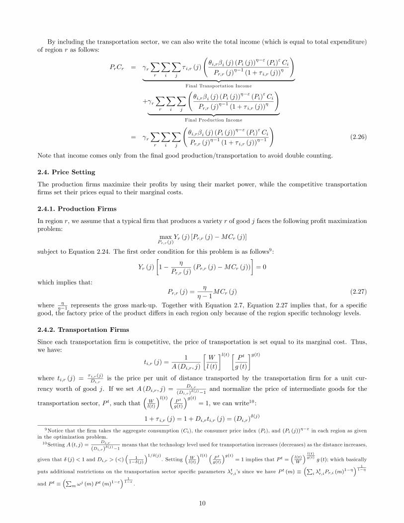
By including the transportation sector, we can also write the total income (which is equal to total expenditure)of region r as follows:
PrCr = rXr
Xi
Xj
� i;r (j)
�i;r�i (j) (Pi (j))
��"(Pi)
"Ci
Pr;r (j)��1
(1 + � i;r (j))�
!| {z }
Final Transportation Income
+ rXr
Xi
Xj
�i;r�i (j) (Pi (j))
��"(Pi)
"Ci
Pr;r (j)��1
(1 + � i;r (j))�
!| {z }
Final Production Income
= rXr
Xi
Xj
�i;r�i (j) (Pi (j))
��"(Pi)
"Ci
Pr;r (j)��1
(1 + � i;r (j))��1
!(2.26)
Note that income comes only from the �nal good production/transportation to avoid double counting.
2.4. Price Setting
The production �rms maximize their pro�ts by using their market power, while the competitive transportation�rms set their prices equal to their marginal costs.
2.4.1. Production Firms
In region r, we assume that a typical �rm that produces a variety r of good j faces the following pro�t maximizationproblem:
maxPr;r(j)
Yr (j) [Pr;r (j)�MCr (j)]
subject to Equation 2.24. The �rst order condition for this problem is as follows9 :
Yr (j)
�1� �
Pr;r (j)(Pr;r (j)�MCr (j))
�= 0
which implies that:Pr;r (j) =
�
� � 1MCr (j) (2.27)
where ���1 represents the gross mark-up. Together with Equation 2.7, Equation 2.27 implies that, for a speci�c
good, the factory price of the product di¤ers in each region only because of the region speci�c technology levels.
2.4.2. Transportation Firms
Since each transportation �rm is competitive, the price of transportation is set equal to its marginal cost. Thus,we have:
ti;r (j) =1
A (Di;r; j)
�W
l (t)
�l(t) �P t
g (t)
�g(t)where ti;r (j) =
� i;r(j)Di;r
is the price per unit of distance transported by the transportation �rm for a unit cur-
rency worth of good j. If we set A (Di;r; j) =Di;r
(Di;r)�(j)�1 and normalize the price of intermediate goods for the
transportation sector, P t, such that�Wl(t)
�l(t) �P t
g(t)
�g(t)= 1, we can write10 :
1 + � i;r (j) = 1 +Di;rti;r (j) = (Di;r)�(j)
9Notice that the �rm takes the aggregate consumption (Ci), the consumer price index (Pi), and (Pi (j))��" in each region as given
in the optimization problem.10Setting A (t; j) =
Di;r
(Di;r)�(j)�1
means that the technology level used for transportation increases (decreases) as the distance increases,
given that � (j) < 1 and Di;r > (<)�
11��(j)
�1=�(j). Setting
�Wl(t)
�l(t) �P t
g(t)
�g(t)= 1 implies that P t =
�l(t)W
� l(t)g(t)
g (t); which basically
puts additional restrictions on the transportation sector speci�c parameters �tr;i�s since we have Pt (m) �
�Pi �
tr;iPr;i (m)
1��� 11��
and P t ��P
m !j (m)P t (m)1�"
� 11�" .
10

which is the mostly used ad hoc gross transportation cost in the literature (see Anderson and van Wincoop 2003,2004, among others). The reason for us to not follow the literature (i.e., the reason for not directly assuming1 + � i;r (j) = (Di;r)
�(j)) is that we want to show the e¤ects of the transportation sector on the national labormarket.
2.5. Interregional (Bilateral) Trade
According to our model, the export of the good j from region r to region i is given by Ci;r (j) +P
mGmi;r (j). By
using region speci�c demand functions, we can write it as follows:
Ci;r (j) +Xm
Gmi;r (j) =�i;r�i (j) (Pi (j))
��"(Pi)
"Ci
Pr;r (j)�(1 + � i;r (j))
� +
Pm !
m (j) (Pm)"Gmi
(1 + � i;r (j)) (Pr;r (j))" (2.28)
Note that the �rst term stands for the �nal good trade, and the second term stands for the intermediate inputtrade. In a special case in which there is only one good produced in each region (�i (j) = 1 and �i;r = �r), and inwhich there is no intermediate input trade at all, after standard calculations, we obtain11 :
(1 + � i;r)Xi;r (j) = �i(Pi)
��1PiCi
(Pr;r (j))��1
((1 + � i;r (j)))��1 (2.29)
where (1 + � i;r)Xi;r (j) = (1 + � i;r)�Ci;r (j) +
PmG
mi;r (j)
�Pr;r (j) is the nominal value of the exports from region
r to region i measured in region i, and PiCi is the total income in region i. Equation 2.29 is the main equation(FOC) that is used to �nd the gravity equation of Anderson-van Wincoop (2003) model. Regardless of the numberof goods produced in each region, compared to our model, Anderson-van Wincoop (2003) model ignores informationcoming from the intermediate input trade, composite price of a good, (Pi (j))
"��, the distribution parameter �i (j),and the di¤erence between " and �. Hence, we can say that the gravity model of Anderson and van Wincoop(2003) is a special case of our model. This result supports Deardor¤�s (1998) remark, "I suspect that just aboutany plausible model of trade would yield something very like the gravity equation...".It is also important to note that our bilateral trade equation (Equation 2.28) includes region and good speci�c
�xed e¤ects that are commonly used in empirical gravity studies, such as Harrigan (1996), Hummels (1999), Reddingand Venables (2004), Rose and van Wincoop (2001) and Anderson and van Wincoop (2003). The next propositiongives further information about the bilateral trade implications of our model.
Proposition 1. The bilateral trade of good j across two regions can be explained by:
� Geographical location, i.e., (1 + � i;r (j)) = (Di;r)�(j), j = 1; :::; J and i = 1; ::; R.
� Population level, i.e., Hi, i = 1; ::; R.
� Taste parameters, i.e., �i (j) and �r;i, i = 1; ::; R and j = 1; :::; J .
� Good speci�c transportation technologies, i.e., � (j), j = 1; :::; J .
� Good/region speci�c production technologies, i.e., Ai (j), j = 1; :::; J and i = 1; ::; R.
P roof. See Equation 3.26 in the next section.
In order to go one step further and �nd the motivation behind our model, we have to obtain an analyticalsolution. The derivation of the closed form solution is given in the next section.
3. Analytical Solution and Implications
In this section, we present the closed form solution of our model and its implications on price levels, consumptionlevels, production levels, bilateral trade levels, and the distribution of labor across production and transportationsectors. We have to restrict ourselves to the special case in which " = 1 to achieve a closed form solution.12 Toobtain the solution, �rst, we solve for the price levels; then, we solve for other variables in terms of Gjr�s and Cr�s;and �nally, we �nd expressions for Gjr�s and Cr�s in terms of exogenous variables.11 In another special case in which � = ", after ignoring the supply side of our model (and thus, intermediate input trade) at all, we
obtain the gravity model in Appendix of Anderson (1979).12Another closed form solution can be obtained by ignoring the intermediate input trade in the model. In such a case, we would not
need the assumption of " = 1.
11
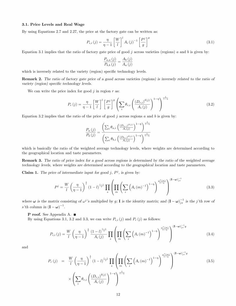
3.1. Price Levels and Real Wage
By using Equations 2.7 and 2.27, the price at the factory gate can be written as:
Pi;i (j) =�
� � 1
�W
l
�lAi (j)
�1�P j
g
�g(3.1)
Equation 3.1 implies that the ratio of factory gate price of good j across varieties (regions) a and b is given by:
Pa;a (j)
Pb;b (j)=Ab (j)
Aa (j)
which is inversely related to the variety (region) speci�c technology levels.
Remark 2. The ratio of factory gate price of a good across varieties (regions) is inversely related to the ratio ofvariety (region) speci�c technology levels.
We can write the price index for good j in region r as:
Pr (j) =�
� � 1
�W
l
�l �P j
g
�g0@Xi
�r;i
(Dr;i)
�(j)
Ai (j)
!1��1A 11��
(3.2)
Equation 3.2 implies that the ratio of the price of good j across regions a and b is given by:
Pa (j)
Pb (j)=
�Pi �a;i
�(Da;i)
�(j)
Ai(j)
�1��� 11��
�Pi �b;i
�(Db;i)
�(j)
Ai(j)
�1��� 11��
which is basically the ratio of the weighted average technology levels, where weights are determined according tothe geographical location and taste parameters.
Remark 3. The ratio of price index for a good across regions is determined by the ratio of the weighted averagetechnology levels, where weights are determined according to the geographical location and taste parameters.
Claim 1. The price of intermediate input for good j, P j , is given by:
P j =W
l
��
� � 1
� 1l
(1� l)l�1l
Ys
0B@Ym
Xi
�Ai (m)
�1�1��!!s(m)
1��
1CA(I�!)�1js
(3.3)
where ! is the matrix consisting of !j�s multiplied by g; I is the identity matrix; and (I� !)�1js is the j�th row ofs�th column in (I� !)�1.
P roof. See Appendix A.By using Equations 3.1, 3.2 and 3.3, we can write Pi;i (j) and Pr (j) as follows:
Pi;i (j) =W
l
��
� � 1
� 1l (1� l)
l�1l
Ai (j)
Ys
0B@Ym
Xi
�Ai (m)
�1�1��!!s(m)
1��
1CA(I�!)�1js g
(3.4)
and
Pr (j) =W
l
��
� � 1
� 1l
(1� l)l�1l
Ys
0B@Ym
Xi
�Ai (m)
�1�1��!!s(m)
1��
1CA(I�!)�1js g
(3.5)
�
0@Xi
�r;i
(Dr;i)
�(j)
Ai (j)
!1��1A 11��
12

Finally, we can write the cost-of-living index for region r as follows:
Pr �W
l
��
� � 1
� 1l
(1� l)l�1l
Yj
0BBBBB@Ys
0@Ym
�Pi
�Ai (m)
�1�1���!s(m)
1��
1A(I�!)�1js g
��P
i �r;i
�(Dr;i)
�(j)
Ai(j)
�1��� 11��
1CCCCCA
�r(j)
(3.6)
Equation 3.6 implies that the ratio of the price of living index across regions a and b is given by:
PaPb=
Yj
0B@Ys
0@Ym
�Pi
�Ai (m)
�1�1���!s(m)
1��
1A(I�!)�1js g �Pi �a;i
�(Da;i)
�(j)
Ai(j)
�1��� 11��
1CA�a(j)
Yj
0B@Ys
0@Ym
�Pi
�Ai (m)
�1�1���!s(m)
1��
1A(I�!)�1js g �Pi �b;i
�(Db;i)
�(j)
Ai(j)
�1��� 11��
1CA�b(j)
which is basically the ratio of the weighted average of technology levels, where weights are again determinedaccording to the geographical location and taste parameters.
Remark 4. The ratio of the price of living index across regions is given by the ratio of the weighted average oftechnology levels, where weights are determined according to the geographical location, factor shares and tasteparameters.
By Equation 3.6, the real wage in region r can be found as:
W
Pr=
l���1�
� 1l
(1� l)1�ll
Yj
0B@Ys
0@Ym
�Pi
�Ai (m)
�1�1���!s(m)
1��
1A(I�!)�1js g �Pi �r;i
�(Dr;i)
�(j)
Ai(j)
�1��� 11��
1CA�r(j)
(3.7)
which says that if the factor share of labor l increases, the real wage in each region increases.
Remark 5. While nominal wage is the same across regions, the real wage in each region di¤ers by its cost-of-livingindex. Moreover, as the factor share of labor l increases, the real wage in each region increases.
3.2. Consumption
By using Equations 2.20 and 3.6, we can write the ratio of consumption across regions a and b as follows:
CaCb
=
HaYj
0B@Ys
0@Ym
�Pi
�Ai (m)
�1�1���!s(m)
1��
1A(I�!)�1js g �Pi �b;i
�(Db;i)
�(j)
Ai(j)
�1��� 11��
1CA�b(j)
HbYj
0B@Ys
0@Ym
�Pi
�Ai (m)
�1�1���!s(m)
1��
1A(I�!)�1js g �Pi �a;i
�(Da;i)
�(j)
Ai(j)
�1��� 11��
1CA�a(j)
(3.8)
which is basically the ratio of the ratio of the population levels multiplied by the weighted average of technologylevels, where weights are determined according to the geographical location and taste parameters. Individual Ci�swill be found later on.
13
Similarly, the ratio of good j consumption across regions a and b is given by:
Ca (j)
Cb (j)=
Ha�a (j)
�Pi �b;i
�(Db;i)
�(j)
Ai(j)
�1��� 11��
Hb�b (j)
�Pi �a;i
�(Da;i)
�(j)
Ai(j)
�1��� 11��
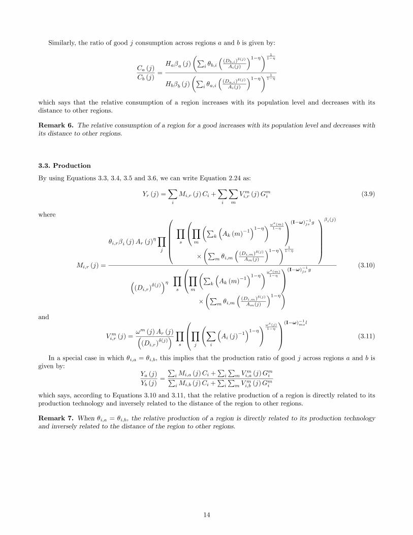
which says that the relative consumption of a region increases with its population level and decreases with itsdistance to other regions.
Remark 6. The relative consumption of a region for a good increases with its population level and decreases withits distance to other regions.
3.3. Production
By using Equations 3.3, 3.4, 3.5 and 3.6, we can write Equation 2.24 as:
Yr (j) =Xi
Mi;r (j)Ci +Xi
Xm
V mi;r (j)Gmi (3.9)
where
Mi;r (j) =
�i;r�i (j)Ar (j)�Yj
0BBBBB@Ys
0@Ym
�Pk
�Ak (m)
�1�1���!s(m)
1��
1A(I�!)�1js g
��P
m �i;m
�(Di;m)
�(j)
Am(j)
�1��� 11��
1CCCCCA
�i(j)
�(Di;r)
�(j)�� Y
s
0@Ym
�Pk
�Ak (m)
�1�1���!s(m)
1��
1A(I�!)�1js g
��P
m �i;m
�(Di;m)
�(j)
Am(j)
�1���(3.10)
and
V mi;r (j) =!m (j)Ar (j)�(Di;r)
�(j)� Y
s
0B@Yj
Xi
�Ai (j)
�1�1��!!s(j)
1��
1CA(I�!)�1msl
(3.11)
In a special case in which �i;a = �i;b, this implies that the production ratio of good j across regions a and b isgiven by:
Ya (j)
Yb (j)=
PiMi;a (j)Ci +
Pi
Pm V
mi;a (j)G
miP
iMi;b (j)Ci +P
i
Pm V
mi;b (j)G
mi
which says, according to Equations 3.10 and 3.11, that the relative production of a region is directly related to itsproduction technology and inversely related to the distance of the region to other regions.
Remark 7. When �i;a = �i;b, the relative production of a region is directly related to its production technologyand inversely related to the distance of the region to other regions.
14
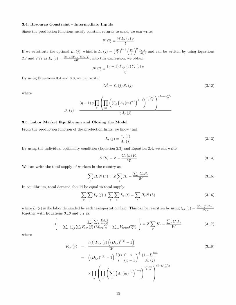
3.4. Resource Constraint - Intermediate Inputs
Since the production functions satisfy constant returns to scale, we can write:
P jGjr =WLr (j) g
l
If we substitute the optimal Lr (j), which is Lr (j) =�Wl
�l�1 �P j
g
�gYr(j)A(j) and can be written by using Equations
2.7 and 2.27 as Lr (j) =(��1)lPr;r(j)Yr(j)
�W , into this expression, we obtain:
P jGjr =(� � 1)Pr;r (j)Yr (j) g
�
By using Equations 3.4 and 3.3, we can write:
Gjr = Yr (j)Sr (j) (3.12)
where
Sr (j) =
(� � 1) gYs
0@Ym
�Pi
�Ai (m)
�1�1���!s(m)
1��
1A(I�!)�1js l
�Ar (j)
3.5. Labor Market Equilibrium and Closing the Model
From the production function of the production �rms, we know that:
Lr (j) =Yr (j)
Ar (j)(3.13)
By using the individual optimality condition (Equation 2.3) and Equation 2.4, we can write:
N (h) = Z � Cr (h)PrW
(3.14)
We can write the total supply of workers in the country as:Xr
HrN (h) = ZXr
Hr �P
r CrPrW
(3.15)
In equilibrium, total demand should be equal to total supply:Xr
Xj
Lr (j) +Xr
Xt
Lr (t) =Xr
HrN (h) (3.16)
where Lr (t) is the labor demanded by each transportation �rm. This can be rewritten by using ti;r (j) =(Di;r)
�(j)�1Di;r
together with Equations 3.13 and 3.7 as:( Pr
PjYr(j)Ar(j)
+P
r
Pj
Pi Fi;r (j) (MirjCi +
Pm VirjmG
mi )
)= Z
Xr
Hr �P
r CrPrW
(3.17)
where
Fi;r (j) =l (t)Pr;r (j)
�(Di;r)
�(j) � 1�
W(3.18)
=�(Di;r)
�(j) � 1� l (t)
l
��
� � 1
� 1l (1� l)
l�1l
Ar (j)
�Ys
0B@Ym
Xi
�Ai (m)
�1�1��!!s(m)
1��
1CA(I�!)�1js g
15
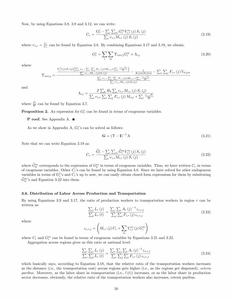
Now, by using Equations 3.8, 3.9 and 3.12, we can write:
Cr =Gjr �
Pi
PmG
mi V
mi;r (j)Sr (j)P
i �i;rMi;r (j)Sr (j)(3.19)
where �i;r = CiCrcan be found by Equation 3.8. By combining Equations 3.17 and 3.19, we obtain:
Gjr =Xi
Xm
�imrjGmi + �rj (3.20)
where
�imrj =
Vmi;r(j)Sr(j)
�Pi �i;r
Pr
Pj Fi;r(j)Mirj+
Pi
�i;rPiW
�P
i �i;rMi;r(j)Sr(j)� 1
Ai(m)Si(m)�P
r
Pj Fi;r (j)VirjmP
i �i;rP
r
Pj Fi;r(j)Mirj+
Pi
�i;rPiWP
i �i;rMi;r(j)Sr(j)
and
�rj =ZP
kHkP
i �i;rMi;r (j)Sr (j)Pi �i;r
Pr
Pj Fi;r (j)Mirj +
Pi�i;rPiW
where PiW can be found by Equation 3.7.
Proposition 2. An expression for Gjr can be found in terms of exogenous variables.
P roof. See Appendix A.
As we show in Appendix A, Gjr�s can be solved as follows:
G = (�� I)�1 � (3.21)
Note that we can write Equation 3.19 as:
Cr =eGjr �Pi
PmeGmi V mi;r (j)Sr (j)P
i �i;rMi;r (j)Sr (j)(3.22)
where eGmk corresponds to the expression of Gmk in terms of exogenous variables. Thus, we have written Cr in termsof exogenous variables. Other Ci�s can be found by using Equation 3.8. Since we have solved for other endogenousvariables in terms of Gji�s and Ci�s up to now, we can easily obtain closed form expressions for them by subsitutingeGmk �s and Equation 3.22 into them.3.6. Distribution of Labor Across Production and Transportation
By using Equations 3.9 and 3.17, the ratio of production workers to transportation workers in region r can bewritten as: P
j Lr (j)Pt Lr (t)
=
Pj
PiAr (j)
�1&i;r;jP
j
Pi Fi;r (j) &i;r;j
(3.23)
where
&i;r;j =
Mi;r (j)Ci +
Xm
V mi;r (j)Gmi
!where Ci and Gmi can be found in terms of exogenous variables by Equations 3.21 and 3.22.Aggregation across regions gives us this ratio at national level:P
r
Pj Lr (j)P
r
Pt Lr (t)
=
Pr
Pj
PiAr (j)
�1&i;r;jP
r
Pj
Pi Fi;r (j) &i;r;j
(3.24)
which basically says, according to Equation 3.18, that the relative ratio of the transportation workers increasesas the distance (i.e., the transportation cost) across regions gets higher (i.e., as the regions get dispersed), ceterisparibus. Moreover, as the labor share in transportation (i.e., l (t)) increases, or as the labor share in productionsector decreases, obviously, the relative ratio of the transportation workers also increases, ceteris paribus.
16

Remark 8. The relative ratio of the transportation workers increases as the distance (i.e., the transportation cost)across regions gets higher (i.e., as the regions get dispersed), or as the labor share in transportation (i.e., l (t))increases, or as the labor share in production sector decreases, ceteris paribus.
3.7. Bilateral Trade
According to Equation 2.28, after using our assumption " = 1, we have:
Ci;r (j) +Xm
Gmi;r (j) =�i;r�i (j) (Pi (j))
��1PiCi
Pr;r (j)�(1 + � i;r (j))
� +
Pm !
m (j)PmGmiPr;r (j) (1 + � i;r (j))
(3.25)
which, according to Equations 3.3, 3.4, 3.5 and 3.6, is equal to:
Ci;r (j) +Xm
Gmi;r (j) =Mi;r (j)Ci +Xm
V mi;r (j)Gmi (3.26)
where Mi;r (j) is given by Equation 3.10, V mi;r (j) is given by Equation 3.11, Ci is given by Equation 3.22, andGmi is given by Equation 3.21. Equation 3.26 tells, according to Equations 3.21 and 3.22, that that the value ofbilateral trade between any two regions depends on the geographic location of all regions, production technology ofthe exporter region together with the technology of other regions, taste parameters of all regions, and good speci�ctransportation technologies.
Claim 3. The ratio of imports of a region across other two regions directly depends on the production technologyratio of the exporters and inversely depends on the distance ratio of the exporters .
P roof. See Appendix A.Equation 3.26 implies that the ratio of imports of region r across regions a and b is given by:
Cr;a (j) +P
mGmr;a (j)
Cr;b (j) +P
mGmr;b (j)
=Mr;a (j)Cr +
Pm V
mr;a (j)G
mr
Mr;b (j)Cr +P
m Vmr;b (j)G
mr
(3.27)
It follows that the ratio of the value of imports of region r across regions a and b is given by:
Xr;a (j)
Xr;b (j)=Pa;a (j)
�Cr;a (j) +
PmG
mr;a (j)
�Pb;b (j)
�Cr;b (j) +
PmG
mr;b (j)
� = �r;aAa(j)��1
(Dr;a)�(j)� + r(j)
(Dr;a)�(j)#r(j)
�r;bAb(j)��1
(Dr;b)�(j)� + r(j)
(Dr;b)�(j)#r(j)
(3.28)
Equation 3.28 says that a region imports more goods (measured in values) from the higher technology regions andless goods from the more distant regions.
Remark 9. A region imports more goods (measured in values) from the higher technology regions and less goodsfrom the more distant regions.
4. Empirical Test
We use the analytical solution of the model to test its empirical power. The model is tested by using four disaggregatedata sets (at the state level) obtained within the U.S., namely consumption, production, trade, and price level, forthe year 2002. As a methodology, �rst, by using the highly accepted parameters used in the literature, we calculatethe predicted values of the model for consumption, production, trade, and price levels; and then we test (compare)them with the data. The data are introduced in the subsections, and their details are described in Appendix B.13
13We use MATLAB Version 7.1.0.246 (R14) Service Pack 3 in our analysis. The data and the codes are available upon request.
17
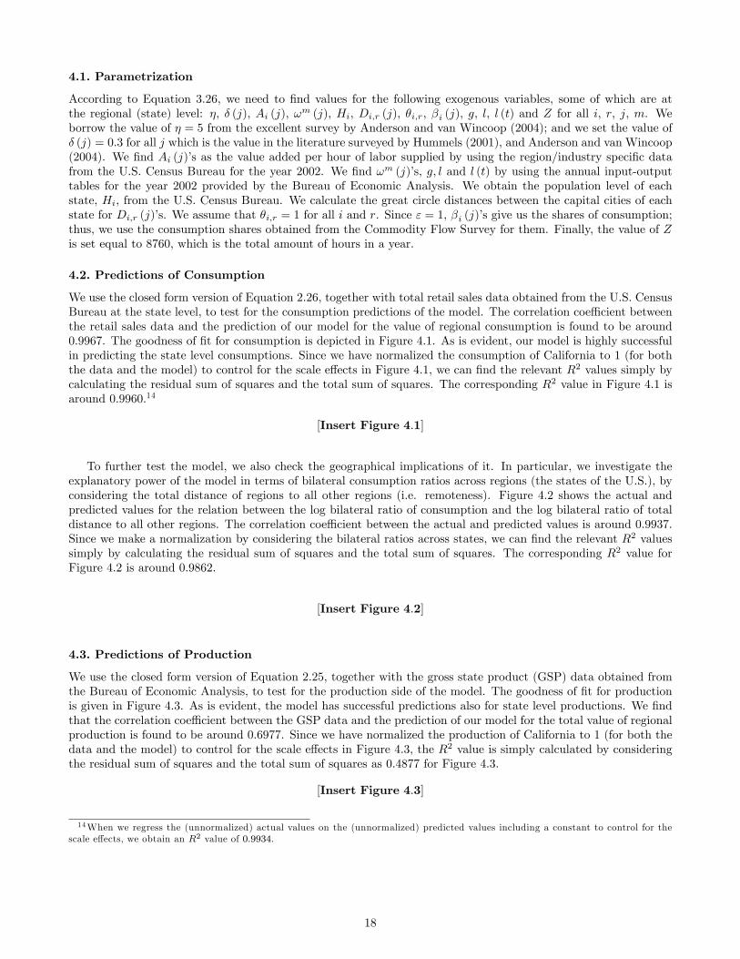
4.1. Parametrization
According to Equation 3.26, we need to �nd values for the following exogenous variables, some of which are atthe regional (state) level: �, � (j), Ai (j), !m (j), Hi, Di;r (j), �i;r, �i (j), g, l, l (t) and Z for all i, r, j, m. Weborrow the value of � = 5 from the excellent survey by Anderson and van Wincoop (2004); and we set the value of� (j) = 0:3 for all j which is the value in the literature surveyed by Hummels (2001), and Anderson and van Wincoop(2004). We �nd Ai (j)�s as the value added per hour of labor supplied by using the region/industry speci�c datafrom the U.S. Census Bureau for the year 2002. We �nd !m (j)�s, g; l and l (t) by using the annual input-outputtables for the year 2002 provided by the Bureau of Economic Analysis. We obtain the population level of eachstate, Hi, from the U.S. Census Bureau. We calculate the great circle distances between the capital cities of eachstate for Di;r (j)�s. We assume that �i;r = 1 for all i and r. Since " = 1, �i (j)�s give us the shares of consumption;thus, we use the consumption shares obtained from the Commodity Flow Survey for them. Finally, the value of Zis set equal to 8760, which is the total amount of hours in a year.
4.2. Predictions of Consumption
We use the closed form version of Equation 2.26, together with total retail sales data obtained from the U.S. CensusBureau at the state level, to test for the consumption predictions of the model. The correlation coe¢ cient betweenthe retail sales data and the prediction of our model for the value of regional consumption is found to be around0:9967. The goodness of �t for consumption is depicted in Figure 4.1. As is evident, our model is highly successfulin predicting the state level consumptions. Since we have normalized the consumption of California to 1 (for boththe data and the model) to control for the scale e¤ects in Figure 4.1, we can �nd the relevant R2 values simply bycalculating the residual sum of squares and the total sum of squares. The corresponding R2 value in Figure 4.1 isaround 0:9960.14
[Insert Figure 4:1]
To further test the model, we also check the geographical implications of it. In particular, we investigate theexplanatory power of the model in terms of bilateral consumption ratios across regions (the states of the U.S.), byconsidering the total distance of regions to all other regions (i.e. remoteness). Figure 4.2 shows the actual andpredicted values for the relation between the log bilateral ratio of consumption and the log bilateral ratio of totaldistance to all other regions. The correlation coe¢ cient between the actual and predicted values is around 0:9937.Since we make a normalization by considering the bilateral ratios across states, we can �nd the relevant R2 valuessimply by calculating the residual sum of squares and the total sum of squares. The corresponding R2 value forFigure 4.2 is around 0:9862.
[Insert Figure 4:2]
4.3. Predictions of Production
We use the closed form version of Equation 2.25, together with the gross state product (GSP) data obtained fromthe Bureau of Economic Analysis, to test for the production side of the model. The goodness of �t for productionis given in Figure 4.3. As is evident, the model has successful predictions also for state level productions. We �ndthat the correlation coe¢ cient between the GSP data and the prediction of our model for the total value of regionalproduction is found to be around 0:6977. Since we have normalized the production of California to 1 (for both thedata and the model) to control for the scale e¤ects in Figure 4.3, the R2 value is simply calculated by consideringthe residual sum of squares and the total sum of squares as 0:4877 for Figure 4.3.
[Insert Figure 4:3]
14When we regress the (unnormalized) actual values on the (unnormalized) predicted values including a constant to control for thescale e¤ects, we obtain an R2 value of 0:9934.
18

We then investigate the explanatory power of the model in terms of bilateral production ratios across the statesof the U.S. by considering total distance of the state to all other regions (i.e. remoteness). Figure 4.4 shows theactual and predicted values for this relation. The correlation coe¢ cient between the actual and predicted valuesis around 0:6775. Since we make a normalization by considering the bilateral ratios across states, we can �nd therelevant R2 values simply by calculating the residual sum of squares and the total sum of squares. The correspondingR2 value for Figure 4.4 is around 0:4464.
[Insert Figure 4:4]
4.4. Predictions of Trade
We use Equation 3.26, together with the Commodity Flow Survey (CFS), which consists of bilateral interstate tradedata within the U.S. at the state level, to test for the trade implications of our model. We consider three di¤erenttrade measures in our analysis, namely trade volume, total exports, and total imports. The goodness of �t for tradevolume is given in Figure 4.5. As is evident, the model has successful predictions also for state level trade volumes.We �nd that the correlation coe¢ cient between the CFS trade data and the prediction of our model for state leveltrade volume is found to be around 0:6295. The R2 value calculated by considering the residual sum of squares andthe total sum of squares is 0:5496 for Figure 4.5.15
[Insert Figure 4:5]
The goodness of �t for total exports is given in Figure 4.6. As is evident, the model has successful predictionsalso for state level exports. We �nd that the correlation coe¢ cient between the CFS trade data and the predictionof our model for state level trade volume is found to be around 0:6710. The R2 value calculated by considering theresidual sum of squares and the total sum of squares is 0:5634 in Figure 4.6.
[Insert Figure 4:6]
The goodness of �t for total imports is given in Figure 4.7. As is evident, the model has successful predictionsalso for state level imports. We �nd that the correlation coe¢ cient between the CFS trade data and the predictionof our model for state level trade volume is found to be around 0:5550. The R2 value calculated by considering theresidual sum of squares and the total sum of squares is 0:4882 in Figure 4.7.
[Insert Figure 4:7]
When we move to Figures 4.8, 4.9 and 4.10, we see the actual and predicted values for the relation between thelog bilateral ratio of total distance to all other regions and the log bilateral ratio of trade volume, total exports andtotal imports, respectively. The corresponding correlation coe¢ cients between the actual and predicted values arearound 0.7077, 0.7983 and 0.5995 for Figures 4.8, 4.9 and 4.10, respectively. Finally, the corresponding R2 valuesfor Figures 4.8, 4.9 and 4.10 are around 0.4641, 0.5677 and 0.3210, respectively.
[Insert Figures 4:8� 4:10]
4.5. Predictions of Price Level
We use Equation 3.6, together with the ACCRA Cost-of-Living Index Data, to test for the price level implicationsof our model. The goodness of �t for price levels is given in Figure 4.11. As is evident, the model has successfulpredictions also for state level trade volumes. We �nd that the correlation coe¢ cient between the ACCRA Cost-of-Living Index data and the prediction of our model for state level price levels is found to be around 0.3194. TheR2 value calculated by considering the residual sum of squares and the total sum of squares is 0.9584 in Figure 4.5.
15When we make the distinction between including and excluding zero trade observations, we �nd that the correlation coe¢ cientbetween the CFS data including the zero trade observations and the prediction of the model is around 0:7004; which corresponds to anR2 value of 0:4906.
19
[Insert Figure 4:11]
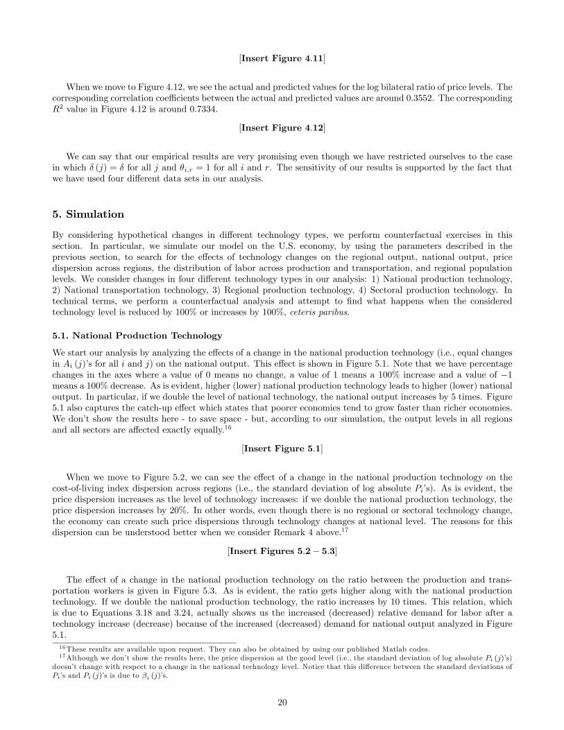
When we move to Figure 4.12, we see the actual and predicted values for the log bilateral ratio of price levels. Thecorresponding correlation coe¢ cients between the actual and predicted values are around 0.3552. The correspondingR2 value in Figure 4.12 is around 0.7334.
[Insert Figure 4:12]
We can say that our empirical results are very promising even though we have restricted ourselves to the casein which � (j) = � for all j and �i;r = 1 for all i and r. The sensitivity of our results is supported by the fact thatwe have used four di¤erent data sets in our analysis.
5. Simulation
By considering hypothetical changes in di¤erent technology types, we perform counterfactual exercises in thissection. In particular, we simulate our model on the U.S. economy, by using the parameters described in theprevious section, to search for the e¤ects of technology changes on the regional output, national output, pricedispersion across regions, the distribution of labor across production and transportation, and regional populationlevels. We consider changes in four di¤erent technology types in our analysis: 1) National production technology,2) National transportation technology, 3) Regional production technology, 4) Sectoral production technology. Intechnical terms, we perform a counterfactual analysis and attempt to �nd what happens when the consideredtechnology level is reduced by 100% or increases by 100%, ceteris paribus.
5.1. National Production Technology
We start our analysis by analyzing the e¤ects of a change in the national production technology (i.e., equal changesin Ai (j)�s for all i and j) on the national output. This e¤ect is shown in Figure 5.1. Note that we have percentagechanges in the axes where a value of 0 means no change, a value of 1 means a 100% increase and a value of �1means a 100% decrease. As is evident, higher (lower) national production technology leads to higher (lower) nationaloutput. In particular, if we double the level of national technology, the national output increases by 5 times. Figure5.1 also captures the catch-up e¤ect which states that poorer economies tend to grow faster than richer economies.We don�t show the results here - to save space - but, according to our simulation, the output levels in all regionsand all sectors are a¤ected exactly equally.16
[Insert Figure 5:1]
When we move to Figure 5.2, we can see the e¤ect of a change in the national production technology on thecost-of-living index dispersion across regions (i.e., the standard deviation of log absolute Pi�s). As is evident, theprice dispersion increases as the level of technology increases: if we double the national production technology, theprice dispersion increases by 20%. In other words, even though there is no regional or sectoral technology change,the economy can create such price dispersions through technology changes at national level. The reasons for thisdispersion can be understood better when we consider Remark 4 above.17
[Insert Figures 5:2� 5:3]
The e¤ect of a change in the national production technology on the ratio between the production and trans-portation workers is given in Figure 5.3. As is evident, the ratio gets higher along with the national productiontechnology. If we double the national production technology, the ratio increases by 10 times. This relation, whichis due to Equations 3.18 and 3.24, actually shows us the increased (decreased) relative demand for labor after atechnology increase (decrease) because of the increased (decreased) demand for national output analyzed in Figure5.1.16These results are available upon request. They can also be obtained by using our published Matlab codes.17Although we don�t show the results here, the price dispersion at the good level (i.e., the standard deviation of log absolute Pi (j)�s)
doesn�t change with respect to a change in the national technology level. Notice that this di¤erence between the standard deviations ofPi�s and Pi (j)�s is due to �i (j)�s.
20

[Insert Figure 5:4]
When we move to Figure 5.4, we can see the e¤ect of a change in the national production technology onthe population dispersion across regions (i.e., the standard deviation of log absolute Hi�s). As is evident, thepopulation dispersion decreases as the level of technology increases: if we double the national production technology,the population dispersion decreases by around 1%. In other words, even though there is no regional or sectoraltechnology change, the economy can create such migrations through technology changes at the national level. Thereasons for this dispersion can be understood better when we consider Figure 5.5 below.
[Insert Figure 5:5]
As is evident in Figure 5.5, the national production technology changes a¤ect the population of di¤erent regionsin di¤erent ways. As an example, while some of highly populated states, such as California and New York, arenegatively a¤ected by a national production technology increase, some low populated states, such as Delaware,Montana, and Maine, are positively a¤ected. These examples give more insight related to Figure 5.4. Nevertheless,we know from Equation 2.23 that these population di¤erences are mostly due to cost-of-living indices. But, what isthe motivation behind the relation between prices and population changes? Figure 5.6 provides information aboutthis issue.
[Insert Figure 5:6]
In particular, Figure 5.6 shows the relation between log bilateral price ratios (i.e., log bilateral Pi ratios) and logbilateral ratios of population changes after an 100% increase in the national production technology. As is evident,the higher the initial price ratios, the lower the ratio of population changes. But what is the exact relation betweenthese two? We answer this question by regressing initial price ratios on the ratio of population changes. We �ndthat the relevant coe¢ cient is �0:08, which suggests on average that if the initial percentage deviation in termsof prices is 100% between any two locations, then the percentage deviation in terms of population changes after a100% increase in the national production technology is going to be 8% less.18
5.2. National Transportation Technology
This subsection depicts the e¤ects of a change in the national transportation technology (i.e., equal changes inelasticities of distance � (j)�s for all j). We start with Figure 5.7 which shows the e¤ect of a change in the nationaltransportation technology on the national output. As is evident, the national output decreases (increases) as thetransportation costs (i.e., � (j)�s for all j) increase (decrease). The interesting point of Figure 5.7. is that asthe transportation costs approach zero, the national output increases by more than 10 times. If we think of ourtransportation costs as regional barriers for a second, our result suggests that decreasing regional barriers (whichcorrespond to national borders in international trade context) leads to welfare gains in a multiplicative manner.Although we don�t show the results here (to save space), this welfare gain is true for all the regions in the economy.19
[Insert Figure 5:7]
When we move to Figure 5.8, we see the e¤ect of a change in the national transportation technology on the cost-of-living index dispersion across regions. As is evident, price dispersion increases (decreases) as the transportationcosts get higher (lower). If we double the transportation costs, the cost-of-living index increases by 80%. Astransportation costs approach zero, the cost-of-living index dispersion decreases by 20%. Thus, transportationcosts are not signi�cant sources of the cost-of-living index dispersion. This result is consistent with the international�nance literature that partly explains the price dispersions through trade costs. Similarly, Figure 5.9 shows thee¤ect of a change in the national transportation technology on the price dispersion at the commodity level (i.e., thestandard deviation of Pi (j)�s). Compared to Figure 5.8, the dispersion in Figure 5.9 shows a di¤erent pattern, bothin terms of second derivatives and in terms of magnitudes. This di¤erence has important implications on appliedresearch based on deviations from law-of-one-price (LOP) or purchasing-power-parity (PPP) comparison analysis.In particular, an applied researcher should be aware of the distinction between aggregate and disaggregate pricelevels according to our model.18The Rbar sqd: for this regression is 0.67.19The magnitude of the welfare gain in each region di¤ers very slightly. These region speci�c results are available upon request, or
they can be obtained by our published Matlab codes.
21
[Insert Figures 5:8� 5:9]
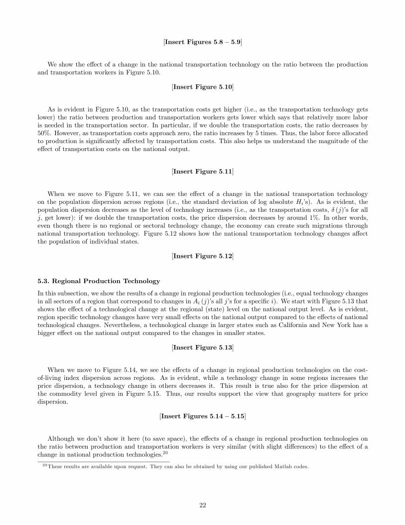
We show the e¤ect of a change in the national transportation technology on the ratio between the productionand transportation workers in Figure 5.10.
[Insert Figure 5:10]
As is evident in Figure 5.10, as the transportation costs get higher (i.e., as the transportation technology getslower) the ratio between production and transportation workers gets lower which says that relatively more laboris needed in the transportation sector. In particular, if we double the transportation costs, the ratio decreases by50%. However, as transportation costs approach zero, the ratio increases by 5 times. Thus, the labor force allocatedto production is signi�cantly a¤ected by transportation costs. This also helps us understand the magnitude of thee¤ect of transportation costs on the national output.
[Insert Figure 5:11]
When we move to Figure 5.11, we can see the e¤ect of a change in the national transportation technologyon the population dispersion across regions (i.e., the standard deviation of log absolute Hi�s). As is evident, thepopulation dispersion decreases as the level of technology increases (i.e., as the transportation costs, � (j)�s for allj, get lower): if we double the transportation costs, the price dispersion decreases by around 1%. In other words,even though there is no regional or sectoral technology change, the economy can create such migrations throughnational transportation technology. Figure 5.12 shows how the national transportation technology changes a¤ectthe population of individual states.
[Insert Figure 5:12]
5.3. Regional Production Technology
In this subsection, we show the results of a change in regional production technologies (i.e., equal technology changesin all sectors of a region that correspond to changes in Ai (j)�s all j�s for a speci�c i). We start with Figure 5.13 thatshows the e¤ect of a technological change at the regional (state) level on the national output level. As is evident,region speci�c technology changes have very small e¤ects on the national output compared to the e¤ects of nationaltechnological changes. Nevertheless, a technological change in larger states such as California and New York has abigger e¤ect on the national output compared to the changes in smaller states.
[Insert Figure 5:13]
When we move to Figure 5.14, we see the e¤ects of a change in regional production technologies on the cost-of-living index dispersion across regions. As is evident, while a technology change in some regions increases theprice dispersion, a technology change in others decreases it. This result is true also for the price dispersion atthe commodity level given in Figure 5.15. Thus, our results support the view that geography matters for pricedispersion.
[Insert Figures 5:14� 5:15]
Although we don�t show it here (to save space), the e¤ects of a change in regional production technologies onthe ratio between production and transportation workers is very similar (with slight di¤erences) to the e¤ect of achange in national production technologies.20
20These results are available upon request. They can also be obtained by using our published Matlab codes.
22
5.4. Sectoral Production Technology
In this subsection, we show the results of a change in sectoral production technologies (i.e., technology changes in aspeci�c industry in all regions which correspond to changes in Ai (j)�s all i�s for a speci�c j). We start with Figure5.16 that shows the e¤ect of a technological change at the sectoral level on the national output. As is evident,di¤erent sectoral technology changes have di¤erent e¤ects on the national output level. In particular, while somesectors such as food-beverage and gasoline have high e¤ects on the national output, some others have a lesser e¤ecton it.
[Insert Figure 5:16]
When we move to Figure 5.17, we see the e¤ects of a change in sectoral production technologies on the cost-of-living index dispersion across regions. As is evident, while a technology change in some sectors increases the pricedispersion, a technology change in some others decreases it.21 In particular, a technological increase in non-durablegoods mostly increases the price dispersion while a technological increase in durable goods mostly decreases theprice dispersion.
[Insert Figure 5:17]
Finally, the e¤ects of a change in sectoral production technologies on the ratio between production and trans-portation workers is given in Figure 5.18. As we see, while some sectors such as gasoline, coal - petroleum, chemicalproducts have a higher e¤ect on the labor ratio, some other have a lesser e¤ect on it.
[Insert Figure 5:18]
6. Conclusions
We have introduced a general equilibrium trade model that considers the distributions of both consumption andproduction at the disaggregate level to analyze the e¤ects of di¤erent technology types on the national and regionalvariables of the U.S. The model relates the trade balance of a state to the geographical location of all regions,income levels of all regions, production levels of all regions, price levels of all regions, as well as the good speci�ctransportation costs and region/good speci�c technology levels. Beyond the gravity models that mostly focus onthe aggregate trade �ow, our model focuses on trade at the disaggregate level. In particular, we show that thegravity models of Anderson (1979) and Anderson and van Wincoop (2003) are special cases of our model.When we solve our model analytically, we go beyond the gravity models and �nd the main determinants of
trade of a region as the geographical location of all regions, population of all regions, taste di¤erences acrossregions, and good speci�c production/transportation technologies. We have also presented the implications ofour model on bilateral ratios of price levels, consumption levels, production levels, bilateral trade volumes, andpopulation levels across regions. In particular, we have shown that the relative production of a region (comparedto other regions) increases with its technology level and decreases with its distance to other regions. Similarly, therelative consumption of a region increases with its population level and its distance to other regions. Moreover, aregion imports more goods from the higher technology regions and fewer goods from the more distant regions. Therelative ratio of the transportation workers increases as the distance across regions gets higher (i.e., as the regionsget dispersed), ceteris paribus.When we test the model empirically, we �nd that it has high explanatory power on the U.S. economy. Finally, we
have simulated the model on the U.S. economy and have shown the e¤ects of a change in technology at the national,regional and sectoral levels. The results have several insights related to output levels, price dispersions, the labormarket, and the regional population levels. In particular, it is shown that if the national production technologylevel is doubled, the output increases by 5 times, the price dispersion increases by 20%, the population dispersiondecreases by 1%, and the ratio of the production labor force to the transportation labor force increases by morethan 10 times As the transportation costs approach zero, the national output increases by more than 10 times, theprice dispersion decreases by 20%, the population dispersion increases by 1%, and the ratio of the production laborforce to the transportation labor force increases by 5 times Finally, region and sector speci�c technology changes
21Although we don�t show the results here, the price dispersion at the commodity level doesn�t change when the sectoral technologieschange. This is mostly due to our parameter assumption that �i;r = 1 for all i and r.
23

have fewer e¤ects on the macroeconomic variables compared to the e¤ects of nationwide technology changes. Aninteresting extension of our paper is to analyze international trade patterns by moving our model to an internationallevel. We are currently working on this project.
24
References
[1] Alvarez, Fernando and Lucas, Robert Jr., (2007), "General equilibrium analysis of the Eaton-Kortum modelof international trade," Journal of Monetary Economics, 54(6): 1726-1768.
[2] Anderson, J.E., (1979), "A Theoretical Foundation for the Gravity Equation", American Economic Review,69(1): 106-116.
[3] Anderson, J.E., and Wincoop, E.V., (2003), "Gravity with Gravitas: A Solution to the Border Puzzle",American Economic Review, 93(1): 170-192.
[4] Anderson, J.E., and Wincoop, E.V., (2004), "Trade Costs", Journal of Economic Literature, 42: 691-751.
[5] Armington, P., (1969), "A theory of Demand for Products Distinguished by Place of Production", IMF Sta¤Papers, 16: 159-178.
[6] Bergstrand, J.H., (1985), "The Gravity Equation in International Trade: Some Microeconomic Foundationsand Empirical Evidence", The Review of Economics and Statistics, 67(3): 474-481.
[7] Bergstrand, J.H., (1989), "The Generalized Gravity Equation, Monopolistic Competition, and the Factor-Proportions Theory in International Trade", The Review of Economics and Statistics, 71(1): 143-153.
[8] Berry, W.D., Fording, R.C., and Hanson, R.L., (2003), "Cost of Living Index for the American States, 1960-2003", Inter-University Consortium for Political and Social Research (ICPSR) Study No: 1275.
[9] Corsetti, G., and Pesenti, P., (2005), "International Dimensions of Optimal Monetary Policy", Journal ofMonetary Economics, 52: 281-305.
[10] Deardor¤, A. V. (1984): �Testing Trade Theories and Predicting Trade Flows,�in Handbook of InternationalEconomics, Volume I, ed. by R. Jones and P. Kenen. Amsterdam: North-Holland.
[11] Deardor¤, A.V., (1998), "Determinants of Bilateral Trade: Does Gravity Work in a Neoclassical World?" inThe Regionalization of the World Economy. J.A. Frankel,ed. Chicago: U. Chicago Press, pp. 7�32.
[12] Dornbusch, R., Fischer, S., and Samuelson, P.A., (1977), "Comparative Advantage, Trade, and Payments in aRicardian Model with a Continuum of Goods", The American Economic Review, 67(5): 823-839. .
[13] Dornbusch, R., Fischer, S., and Samuelson, P.A., (1980), "Heckscher-Ohlin Trade Theory with a Continuumof Goods", Quarterly Journal of Economics, 95(2): 203-224.
[14] Eaton, J., and Kortum, S., (2002), "Technology, Geography and Trade", Econometrica, 70(5): 1741-1779.
[15] Evenett, S. J., and W. Keller (2002): �On Theories Explaining the Success of the Gravity Equation,�Journalof Political Economy, 110, 281�316.
[16] Erceg, C.J., Henderson, D.W., and Levin A.T., (2000), "Optimal Monetary Policy with Staggered Wage andPrice Contracts", Journal of Monetary Economics, 46: 281-313.
[17] Gali, J. and Monacelli, T., (2005), "Monetary Policy and Exchange Rate Volatility in a Small Open Economy",Review of Economic Studies, 72: 707-734.
[18] Gallaway, Michael P. , McDaniel, Christine A., and Rivera, Sandra A., (2003), "Short-run and long-runindustry-level estimates of U.S. Armington elasticities", North American Journal of Economics and Finance14: 49�68
[19] Grossman, G. M., and E. Helpman (1995): �Technology and Trade,� in The Handbook of International Eco-nomics, Volume III, ed. by G. M. Grossman and K. Rogo¤. Amsterdam: North-Holland.
[20] Harrigan, J., (1996), "Openness to Trade in Manufactures in the OECD", Journal of International Economics,40: 23-39.
[21] Helpman, E. (1987): �Imperfect Competition and International Trade: Evidence from Fourteen IndustrialCountries,�Journal of Japanese and International Economics, 1: 62�81.
25
[22] Hummels, D., (1999), "Have International Transportation Costs Declined?", mimeo.
[23] Hummels, D., (2001), "Toward a Geography of Trade Costs", mimeo.
[24] Hummels, D., and J. Levinsohn (1995):�Monopolistic Competition and International Trade: Reconsidering theEvidence,�Quarterly Journal of Economics, 110: 799�836.
[25] Jensen, P. E. (2000), �Analysis of Bilateral Trade Patterns with Panel Data,�Review of International Eco-nomics, 8: 86�99.
[26] Kehoe, T.J., (2003), "An Evaluation of the Performance of Applied General Equilibrium Models of the Impactof NAFTA", mimeo.
[27] Krugman, P., (1980), "Scale Economies, Product Di¤erentiation, and the Pattern of Trade", American Eco-nomic Review, 70(5): 950-959.
[28] Krugman, P., (1991), "Increasing Returns and Economic Geography", Journal of Political Economy, 99(3):483-499.
[29] Lopez, Rigoberto A., Pagoulatos, Emilio, Gonzalez, Maria A., (2006), "Home bias and U.S. imports of processedfood products", North American Journal of Economics and Finance 17: 363�373
[30] Matsuyama, K., (2000), "A Ricardian Model with a Continuum of Goods under Nonhomothetic Preferences:Demand Complementarities, Income Distribution, and North-South Trade", Journal of Political Economy,108(6): 1093-1120.
[31] Rauch, J. E. (1999): �Networks vs. Markets in International Trade,�Journal of International Economics, 48,7�35.
[32] Redding, S. and Venables, A.J., (2004)"Economic Geography and International Inequality", Journal of Inter-national Economics, 62(1): 53-82.
[33] Rose, A.K. and Wincoop, E.V., (2001), "National Money as a Barrier to Trade: The Real Case for CurrencyUnion", American Economic Review Papers and Proceedings 91(2): 386�90.
[34] Rossi-Hansberg, E., (2005), "A Spatial Theory of Trade", American Economic Review, 95(5): 1464-1491.
[35] Suga, Nobuhito, (2007), "A monopolistic-competition model of international trade with external economies ofscale", North American Journal of Economics and Finance 18: 77�91
[36] Wei, SJ, (1996), "Intranational versus International Trade: How Stubborn are Nations in Global Integration?",NBER Working Paper No: 5531.
[37] Yilmazkuday, H., (2007), "In�ation Targeting Supported by Managed Exchange Rate", Applied Economics,39(16): 2011-2026.
[38] Yilmazkuday, H., (2008a), "Understanding Interstate Trade Patterns". Available at SSRN:http://ssrn.com/abstract=995542
[39] Yilmazkuday, H., (2008b), "Distribution of Consumption, Production and Trade within the U.S.". Availableat SSRN: http://ssrn.com/abstract=995536
26
Appendix A - ProofsProof of Claim 1. By using Equations 2.7, 2.10, 2.11 and 2.27, together with " = 1, we can write:
P j (m) � �
� � 1
�W
l
�l �Pm
g
�g Xi
Ai (m)��1! 1
1��
and
P j � Y
m
(Pm)g!j(m)
!�g�g
� � 1
�W
l
�l0B@Ym
Xi
�Ai (m)
�1�1��!!j(m)
1��
1CAIf we take the logs of both sides, we obtain:
pj �Xm
g!j (m) pm + kj
where
kj = log
0B@ �g�g� � 1
�W
l
�l0B@Ym
Xi
�Ai (m)
�1�1��!!j(m)
1��
1CA1CA
and pj = logP j . In matrix form, we can write:
p = !p+ k
where
p =
0BB@p1
��pJ
1CCA ; ! =0BB@
g!1 (1) g!1 (J)� � �� � �
g!J (1) g!J (J)
1CCA ; k =0BB@
k1��kJ
1CCAThis system can be solved as:
p = (I� !)�1 k
where I represents the identity matrix and j�th row of (I� !)�1 k corresponds to pj . Thus, P j�s can easily befound by
P j = exp�(I� !)�1j kj
�=
Ys
(Ks)(I�!)�1js
where Km = exp(km); (I� !)�1j is the j�th row of (I� !)�1 ; and (I� !)�1jm is the j�th row of m�th column in
(I� !)�1.Since
Ks =
0B@ �g�g� � 1
�W
l
�l0B@Ym
Xi
�Ai (m)
�1�1��!!s(m)
1��
1CA1CA
we can obtain:
P j =Ys
0B@0B@ �g�g� � 1
�W
l
�l0B@Ym
Xi
�Ai (m)
�1�1��!!s(m)
1��
1CA1CA1CA(I�!)�1js
which can be rewritten as:
P j =W
l
��
� � 1
� 1l
(1� l)l�1l
Ys
0B@Ym
Xi
�Ai (m)
�1�1��!!s(m)
1��
1CA(I�!)�1js
27
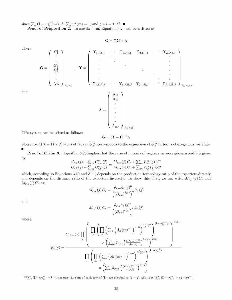
sinceP
s (I� !)�1js = l
�1;P
s !s (m) = 1; and g + l = 1. 22
Proof of Proposition 2. In matrix form, Equation 3.20 can be written as:
G = �G+ �
where
G =
0BBBBBBBBBB@
G11��GJ1G12��GJR
1CCCCCCCCCCARJ�1
; � =
0BBBBBBBBBB@
�1;1;1;1 � � �1;J;1;1 �2;1;1;1 � � �R;J;1;1� � �� � �� � �� � �� � �� � �
�1;1;R;J � � �1;J;R;J �2;1;R;J � � �R;J;R;J
1CCCCCCCCCCARJ�RJ
and
� =
0BBBBBBBBBB@
�11�12�����
�RJ
1CCCCCCCCCCARJ�R
This system can be solved as follows:G = (�� I)�1 �
where row (((k � 1)� J) +m) of G, say eGmk ; corresponds to the expression of Gmk in terms of exogenous variables.Proof of Claim 3. Equation 3.26 implies that the ratio of imports of region r across regions a and b is given
by:Cr;a (j) +
PmG
mr;a (j)
Cr;b (j) +P
mGmr;b (j)
=Mr;a (j)Cr +
Pm V
mr;a (j)G
mr
Mr;b (j)Cr +P
m Vmr;b (j)G
mr
which, according to Equations 3.10 and 3.11, depends on the production technology ratio of the exporters directlyand depends on the distance ratio of the exporters inversely. To show this, �rst, we can write Mr;a (j)Cr andMr;b (j)Cr as:
Mr;a (j)Cr =�r;aAa (j)
��(Dr;a)
�(j)�� #r (j)
and
Mr;b (j)Cr =�r;bAb (j)
��(Dr;b)
�(j)�� #r (j)
where
#r (j) =
Cr�r (j)Yj
0BBBBB@Ys
0@Ym
�Pk
�Ak (m)
�1�1���!s(m)
1��
1A(I�!)�1js g
��P
m �r;m
�(Dr;m)
�(j)
Am(j)
�1��� 11��
1CCCCCA
�r(j)
Ys
0@Ym
�Pk
�Ak (m)
�1�1���!s(m)
1��
1A(I�!)�1js g
��P
m �r;m
�(Dr;m)
�(j)
Am(j)
�1���22P
s (I� !)�1js = l�1, because the sum of each row of (I� !) is equal to (1� g), and thus,
Ps (I� !)
�1js = (1� g)�1.
28

where Cr is again given by Equations 3.22. Similarly, we can writeP
m Vmr;a (j)G
mr and
Pm V
mr;b (j)G
mr as:
Xm
V mr;a (j)Gmr =
Aa (j)�(Dr;a)
�(j)�r (j)
and Xm
V mr;b (j)Gmr =
Ab (j)�(Dr;b)
�(j)�r (j)
where
r (j) =Xm
Gmr !m (j)
Ys
0B@Yj
Xi
�Ai (j)
�1�1��!!s(j)
1��
1CA(I�!)�1msl
where Gmr is again given by Equation 3.21. Thus, we can rewrite Equation 3.27 as:
Cr;a (j) +P
mGmr;a (j)
Cr;b (j) +P
mGmr;b (j)
=
�r;aAa(j)�
(Dr;a)�(j)� +
Aa(j)
(Dr;a)�(j)
r(j)#r(j)
�r;bAb(j)�
(Dr;b)�(j)� +
Ab(j)
(Dr;b)�(j)
r(j)#r(j)
Hence, we have shown our claim.
29
Appendix B - DataFor the value of consumption in each state, we use the retail trade data for the year 2002, of which North
American Industry Classi�cation System (NAICS) code is 44-45. For the value of production in each state, we usegross state product (GSP) obtained from the Bureau of Economic Analysis for the year 2002. For the bilateral tradeanalysis, we use the state-level Commodity Flow Survey (CFS) data obtained from the Bureau of TransportationStatistics for the United States for the year 2002. In particular, we use the interstate trade data for the 2-digitStandard Classi�cation of Transported Goods (SCTG) commodities of which codes and names are given in TableA.1 together with the corresponding NAICS code that is used to �nd the region/sector speci�c technology levels.The source for the crosswalk between NAICS and SCTG is National Transportation Library of the Bureau ofTransportation Statistics.Because of the data availability, we include all the states of the United States except for Alaska, District of
Columbia and Hawaii. In order to obtain the technology levels, we �rst use an approximate crosswalk between3-digit North American Industry Classi�cation System (NAICS) and 2-digit SCTG obtained from the NationalTransportation Library of the Bureau of Transportation Statistics. This crosswalk is given by Table A.1.. After
that, we use Ai (j) = log�
Vi(j)PiLi(j)
�as our proxy for the technology levels, where Vi (j) is the industry/region
speci�c value added; Pi is the cost-of-living index for state i borrowed from Berry et al. (2003); and Li (j) is theindustry/region speci�c hours of labor supplied by the production workers. For the value added of each NAICSindustry in each state, we use the state level U.S. Census Bureau data for the relevant industries in 2002.For the distance measures, we calculate the great circle distance between states by using the latitudes and the
longitudes of the capital cities of each state published by U.S. Census Bureau. Note that we don�t use the averagedistance measures given by CFS, because those measures are available only for the realized trades across states.Since we include zero observations (i.e., no trade across states) into our analysis, we use the great circle distancemeasures that are not included in CFS.The cost-of-living index of Berry et al. (2003) has been used in calculating the technology levels above, because
they represent a composite price index including both traded and non-traded goods. However, since our modelconsiders only traded goods, we need a more accurate measure of cost-of-living index, which mostly covers theprices of traded goods. In this sense, for cost-of-living index in each region, we use the price index for traded goods(i.e., grocery index) of the ACCRA cost-of-living index for the year 2002. Since ACCRA cost-of-living index isrepresented at city level within the U.S., we consider the cost-of-living index in the capital city of each state as astate level measure. This is also consistent with using the location of capital cities in calculating the great circledistances across states.
30
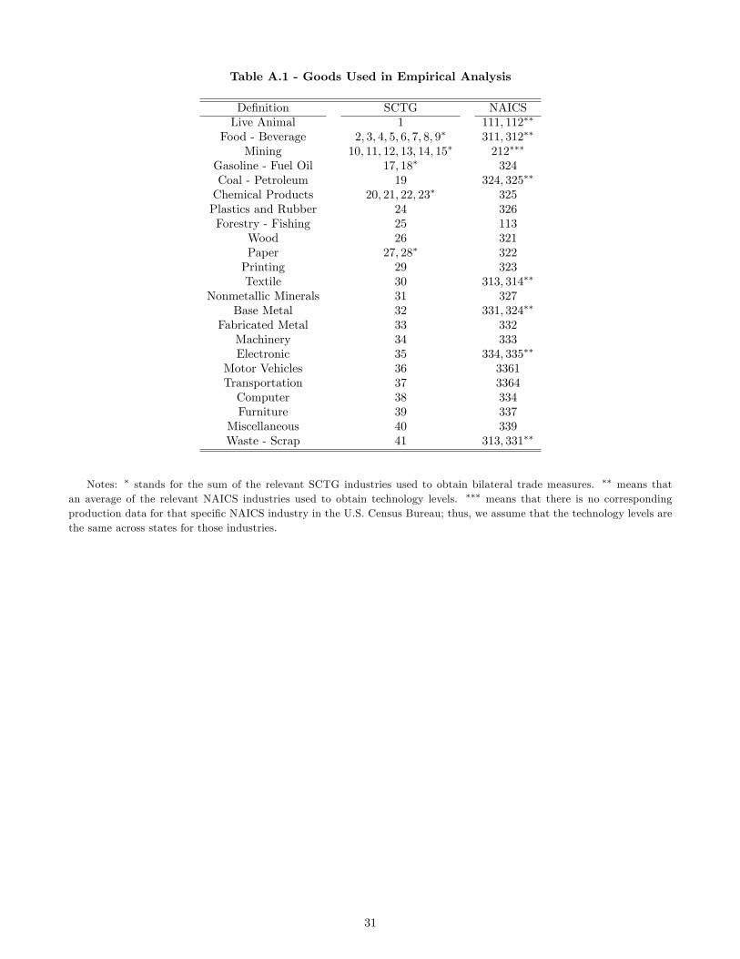
Table A.1 - Goods Used in Empirical Analysis
De�nition SCTG NAICSLive Animal 1 111; 112��
Food - Beverage 2; 3; 4; 5; 6; 7; 8; 9� 311; 312��
Mining 10; 11; 12; 13; 14; 15� 212���
Gasoline - Fuel Oil 17; 18� 324Coal - Petroleum 19 324; 325��
Chemical Products 20; 21; 22; 23� 325Plastics and Rubber 24 326Forestry - Fishing 25 113
Wood 26 321Paper 27; 28� 322Printing 29 323Textile 30 313; 314��
Nonmetallic Minerals 31 327Base Metal 32 331; 324��
Fabricated Metal 33 332Machinery 34 333Electronic 35 334; 335��
Motor Vehicles 36 3361Transportation 37 3364Computer 38 334Furniture 39 337
Miscellaneous 40 339Waste - Scrap 41 313; 331��
Notes: � stands for the sum of the relevant SCTG industries used to obtain bilateral trade measures. �� means thatan average of the relevant NAICS industries used to obtain technology levels. ��� means that there is no correspondingproduction data for that speci�c NAICS industry in the U.S. Census Bureau; thus, we assume that the technology levels arethe same across states for those industries.
31
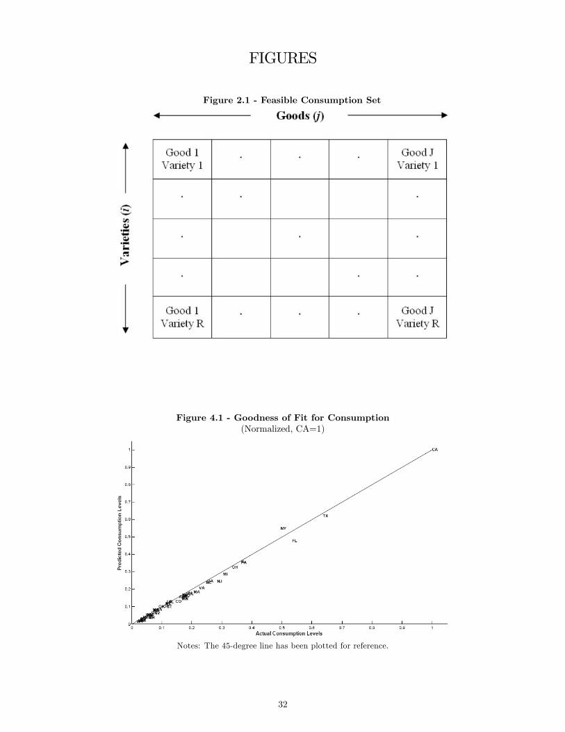
FIGURES
Figure 2.1 - Feasible Consumption Set
Figure 4.1 - Goodness of Fit for Consumption(Normalized, CA=1)
Notes: The 45-degree line has been plotted for reference.
32
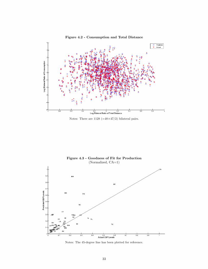
Figure 4.2 - Consumption and Total Distance
Notes: There are 1128 (=48�47/2) bilateral pairs.
Figure 4.3 - Goodness of Fit for Production(Normalized, CA=1)
Notes: The 45-degree line has been plotted for reference.
33

Figure 4.4 - Production and Total Distance
Notes: There are 1128 (=48�47/2) bilateral pairs.
Figure 4.5 - Goodness of Fit for Trade Volume(Normalized, CA=1)
Notes: The 45-degree line has been plotted for reference.
34
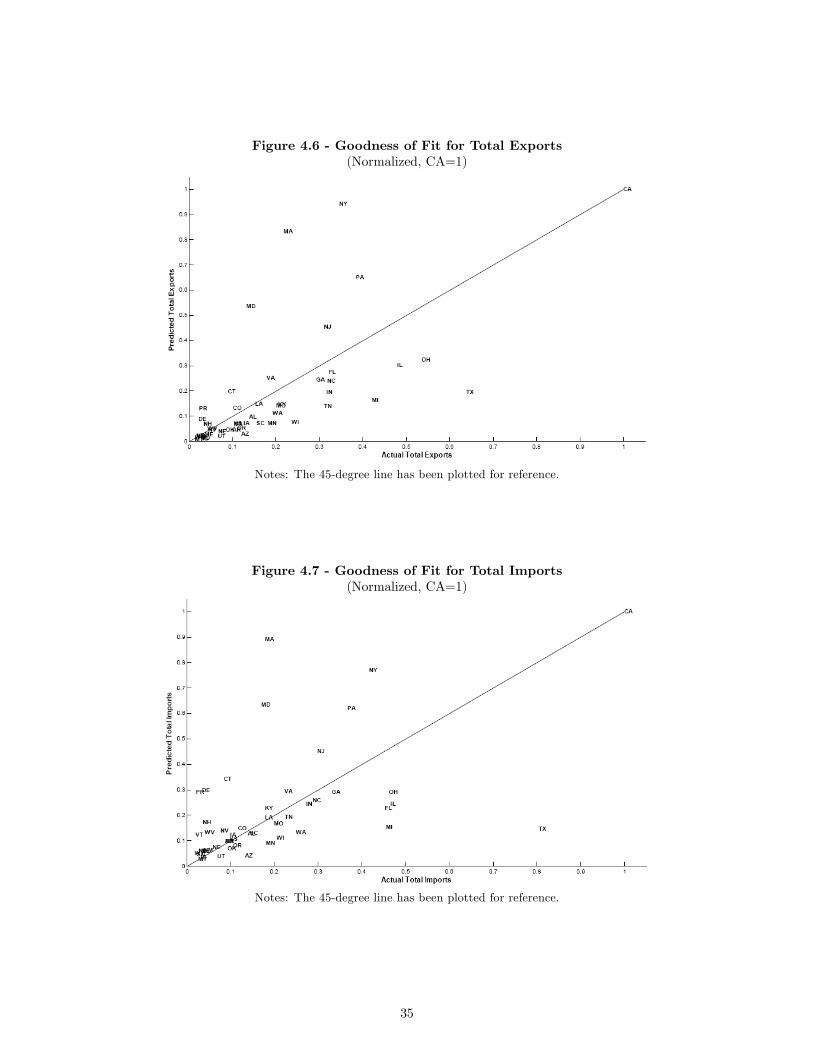
Figure 4.6 - Goodness of Fit for Total Exports(Normalized, CA=1)
Notes: The 45-degree line has been plotted for reference.
Figure 4.7 - Goodness of Fit for Total Imports(Normalized, CA=1)
Notes: The 45-degree line has been plotted for reference.
35

Figure 4.8 - Trade Volume and Total Distance
Notes: There are 1128 (=48�47/2) bilateral pairs.
Figure 4.9 - Total Exports and Total Distance
Notes: There are 1128 (=48�47/2) bilateral pairs.
36

Figure 4.10 - Total Imports and Total Distance
Notes: There are 1128 (=48�47/2) bilateral pairs.
Figure 4.11 - Goodness of Fit for Price Levels(Normalized, CA=1)
Notes: The 45-degree line has been plotted for reference.
37
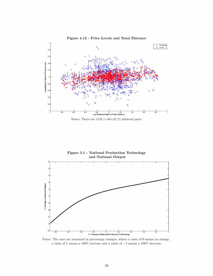
Figure 4.12 - Price Levels and Total Distance
Notes: There are 1128 (=48�47/2) bilateral pairs.
Figure 5.1 - National Production Technologyand National Output
Notes: The axes are measured in percentage changes, where a value of 0 means no change,a value of 1 means a 100% increase and a value of �1 means a 100% decrease.
38
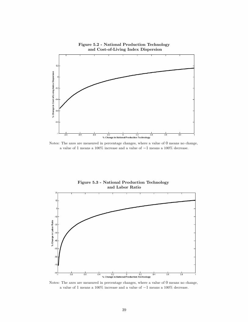
Figure 5.2 - National Production Technologyand Cost-of-Living Index Dispersion
Notes: The axes are measured in percentage changes, where a value of 0 means no change,a value of 1 means a 100% increase and a value of �1 means a 100% decrease.
Figure 5.3 - National Production Technologyand Labor Ratio
Notes: The axes are measured in percentage changes, where a value of 0 means no change,a value of 1 means a 100% increase and a value of �1 means a 100% decrease.
39
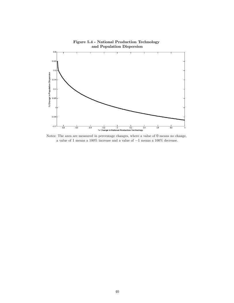
Figure 5.4 - National Production Technologyand Population Dispersion
Notes: The axes are measured in percentage changes, where a value of 0 means no change,a value of 1 means a 100% increase and a value of �1 means a 100% decrease.
40

Figure 5.5 - National Production Technologyand Regional Population Levels
Notes: The axes are measured in percentage changes, where a value of 0 means no change,a value of 1 means a 100% increase and a value of �1 means a 100% decrease.
41

Figure 5.6 - Initial Prices and Population ChangesAfter a 100% Increase in National Production Technology
Notes: The axes are measured in percentage changes, where a value of 0 means no change,a value of 1 means a 100% increase and a value of �1 means a 100% decrease.
Figure 5.7 - Transportation Costs and National Output
Notes: The axes are measured in percentage changes, where a value of 0 means no change,a value of 1 means a 100% increase and a value of �1 means a 100% decrease.
42
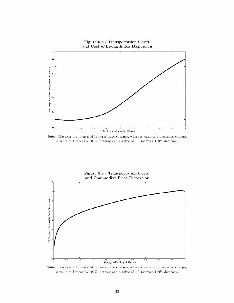
Figure 5.8 - Transportation Costsand Cost-of-Living Index Dispersion
Notes: The axes are measured in percentage changes, where a value of 0 means no change,a value of 1 means a 100% increase and a value of �1 means a 100% decrease.
Figure 5.9 - Transportation Costsand Commodity Price Dispersion
Notes: The axes are measured in percentage changes, where a value of 0 means no change,a value of 1 means a 100% increase and a value of �1 means a 100% decrease.
43
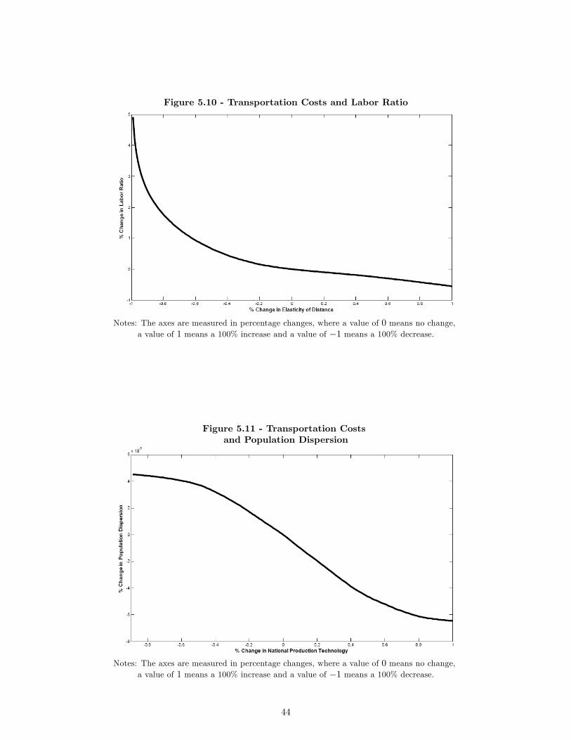
Figure 5.10 - Transportation Costs and Labor Ratio
Notes: The axes are measured in percentage changes, where a value of 0 means no change,a value of 1 means a 100% increase and a value of �1 means a 100% decrease.
Figure 5.11 - Transportation Costsand Population Dispersion
Notes: The axes are measured in percentage changes, where a value of 0 means no change,a value of 1 means a 100% increase and a value of �1 means a 100% decrease.
44

Figure 5.12 - National Production Technologyand Regional Population Levels
Notes: The axes are measured in percentage changes, where a value of 0 means no change,a value of 1 means a 100% increase and a value of �1 means a 100% decrease.
45

Figure 5.13 - Regional Production Technologyand National Output
Notes: The axes are measured in percentage changes, where a value of 0 means no change,a value of 1 means a 100% increase and a value of �1 means a 100% decrease.
46

Figure 5.14 - Regional Production Technologyand Cost-of-Living Index Dispersion
Notes: The axes are measured in percentage changes, where a value of 0 means no change,a value of 1 means a 100% increase and a value of �1 means a 100% decrease.
47
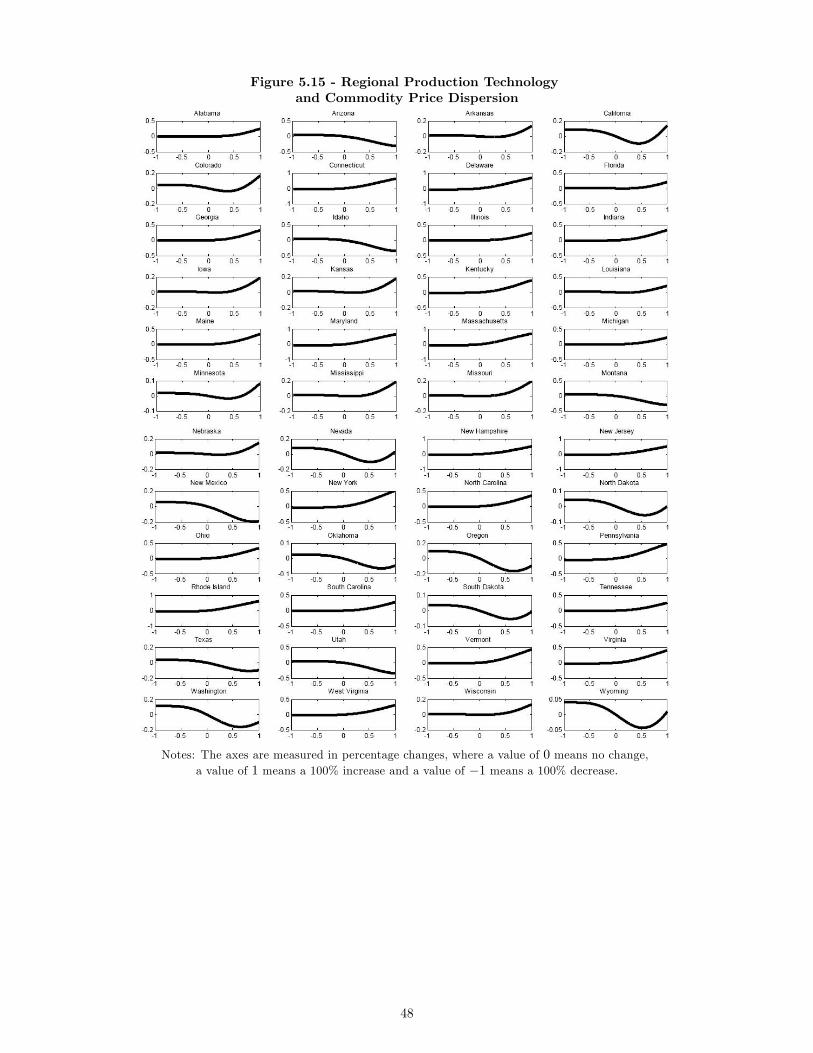
Figure 5.15 - Regional Production Technologyand Commodity Price Dispersion
Notes: The axes are measured in percentage changes, where a value of 0 means no change,a value of 1 means a 100% increase and a value of �1 means a 100% decrease.
48
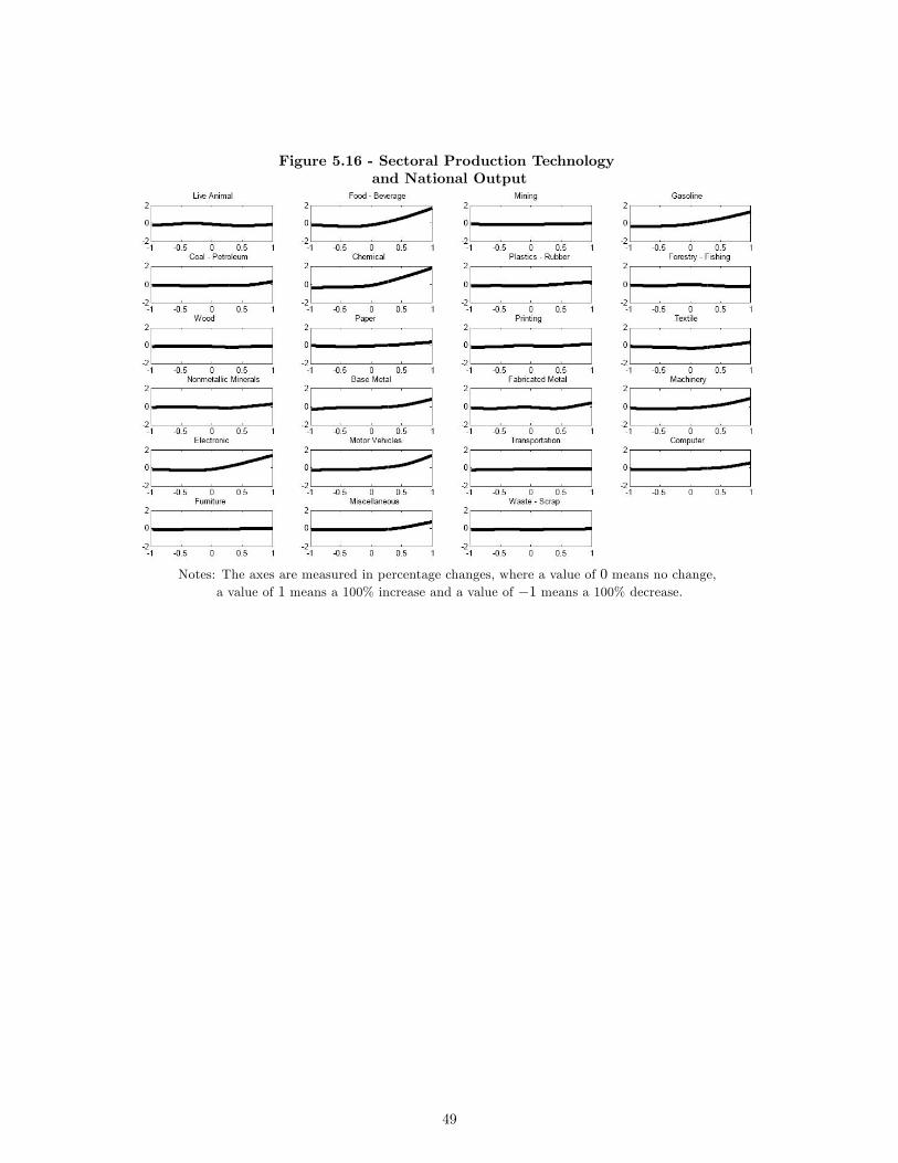
Figure 5.16 - Sectoral Production Technologyand National Output
Notes: The axes are measured in percentage changes, where a value of 0 means no change,a value of 1 means a 100% increase and a value of �1 means a 100% decrease.
49

Figure 5.17 - Sectoral Production Technologyand Cost-of-Living Index Dispersion
Notes: The axes are measured in percentage changes, where a value of 0 means no change,a value of 1 means a 100% increase and a value of �1 means a 100% decrease.
50

Figure 5.18 - Sectoral Production Technologyand Labor Ratio
Notes: The axes are measured in percentage changes, where a value of 0 means no change,a value of 1 means a 100% increase and a value of �1 means a 100% decrease.
51


