Response to Harmonic Excitation

Part 1 : Undamped Systems

Harmonic excitation refers to a sinusoidal external force of a certain frequency applied to a

system. The response of a system to harmonic excitation is a very important topic because it is

encountered very commonly and also covers the concept of resonance. Resonance occurs

when the external excitation has the same frequency as the natural frequency of the system. It

leads to large displacements and can cause a system to exceed its elastic range and fail

structurally. A popular example, that many people are familiar with, is that of a singer breaking

a glass by singing. Harmonic excitation is also commonly observed in systems that contain a

rotating mass for example tires, engines, rotors, etc. This module develops the equations for

the response of a single-degree-of-freedom system without damping to harmonic excitation

using a spring-mass model. The next module will continue by including damping in the system

model.

Harmonic Excitation of Undamped Systems

Fig. 1: Spring- mass system with an external force.

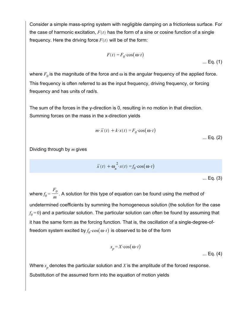
Consider a simple mass-spring system with negligible damping on a frictionless surface. For

the case of harmonic excitation, has the form of a sine or cosine function of a single

frequency. Here the driving force will be of the form:

... Eq. (1)

where is the magnitude of the force and is the angular frequency of the applied force.

This frequency is often referred to as the input frequency, driving frequency, or forcing

frequency and has units of rad/s.

The sum of the forces in the y-direction is 0, resulting in no motion in that direction.

Summing forces on the mass in the x-direction yields

... Eq. (2)

Dividing through by gives

... Eq. (3)

where . A solution for this type of equation can be found using the method of

undetermined coefficients by summing the homogeneous solution (the solution for the case

) and a particular solution. The particular solution can often be found by assuming that

it has the same form as the forcing function. That is, the oscillation of a single-degree-of-

freedom system excited by is observed to be of the form

... Eq. (4)

Where denotes the particular solution and is the amplitude of the forced response.

Substitution of the assumed form into the equation of motion yields

... Eq. (5)

Factoring out and solving for gives

... Eq. (6)

provided that is not zero. Therefore as long as the driving and natural frequencies

are not equal the particular solution will be of the form

... Eq. (7)

Since the system is linear, the total solution is the sum of the particular solution and the

homogeneous solution

... Eq. (8)

Recalling that can be represented as , the total

solution can be expressed in the form

... Eq. (9)

With constants of integration and . These are determined by initial conditions. Let the

initial position and velocity be given by constants and . Then

... Eq. (10)and

... Eq. (11)

Solving the above two equations for and and substituting these values into Eq. (9) yields the total response

... Eq. (12)

For example, the following plot shows the response of an undamped system with

rad/s, m and m/s to harmonic excitation of magnitude N/kg at rad/s and rad/s.

plotplot

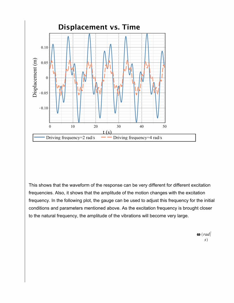
This shows that the waveform of the response can be very different for different excitation

frequencies. Also, it shows that the amplitude of the motion changes with the excitation

frequency. In the following plot, the gauge can be used to adjust this frequency for the initial

conditions and parameters mentioned above. As the excitation frequency is brought closer

to the natural frequency, the amplitude of the vibrations will become very large.

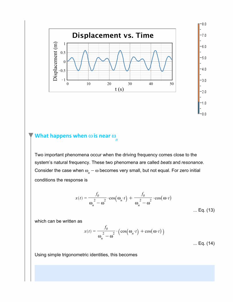
What happens when is near

Two important phenomena occur when the driving frequency comes close to the

beats and resonance.

Consider the case when becomes very small, but not equal. For zero initial

conditions the response is

... Eq. (13)

which can be written as

... Eq. (14)

Using simple trigonometric identities, this becomes

... Eq. (15)

Since is small, is large by comparison and the term

oscillates with a much longer period than does . Recall that the period of

oscillation T is defined as

... Eq. (16)or in this case

.. Eq. (17)

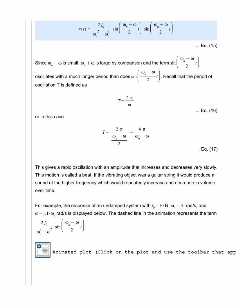
This gives a rapid oscillation with an amplitude that increases and decreases very slowly.

This motion is called a beat. If the vibrating object was a guitar string it would produce a

sound of the higher frequency which would repeatedly increase and decrease in volume

over time.

For example, the response of an undamped system with N, rad/s, and

rad/s is displayed below. The dashed line in the animation represents the term

.

Animated plot (Click on the plot and use the toolbar that appears above to play the animation)Animated plot (Click on the plot and use the toolbar that appears above to play the animation)

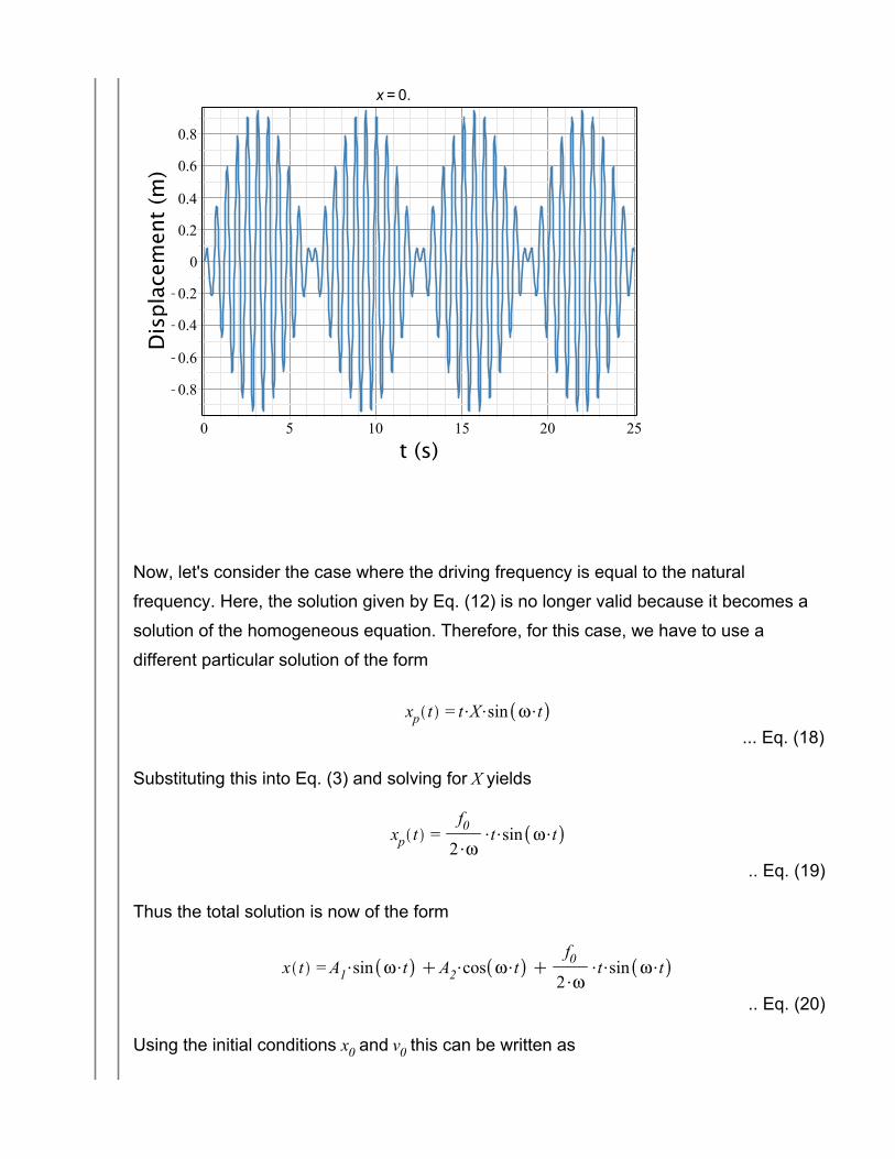
Now, let's consider the case where the driving frequency is equal to the natural

frequency. Here, the solution given by Eq. (12) is no longer valid because it becomes a

solution of the homogeneous equation. Therefore, for this case, we have to use a

different particular solution of the form

... Eq. (18)

Substituting this into Eq. (3) and solving for yields

.. Eq. (19)

Thus the total solution is now of the form

.. Eq. (20)

Using the initial conditions and this can be written as

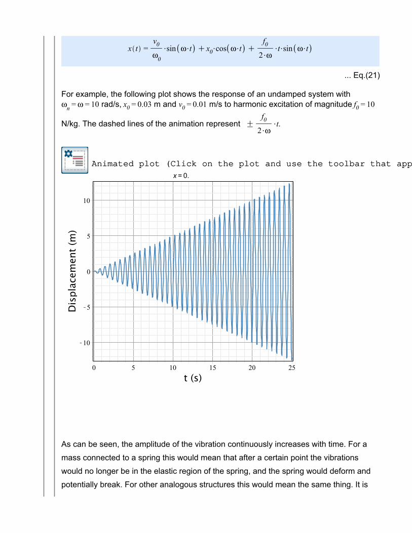
... Eq.(21)

For example, the following plot shows the response of an undamped system with rad/s, m and m/s to harmonic excitation of magnitude

N/kg. The dashed lines of the animation represent .

Animated plot (Click on the plot and use the toolbar that appears above to play the animation)Animated plot (Click on the plot and use the toolbar that appears above to play the animation)

As can be seen, the amplitude of the vibration continuously increases with time. For a

mass connected to a spring this would mean that after a certain point the vibrations

would no longer be in the elastic region of the spring, and the spring would deform and

potentially break. For other analogous structures this would mean the same thing. It is

very important to understand this phenomena because it can be very dangerous for

structures and systems.

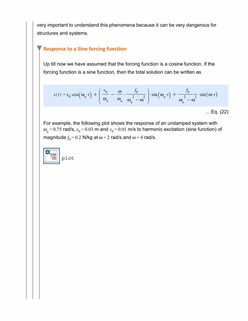
Response to a Sine forcing function

Up till now we have assumed that the forcing function is a cosine function. If the

forcing function is a sine function, then the total solution can be written as

... Eq. (22)

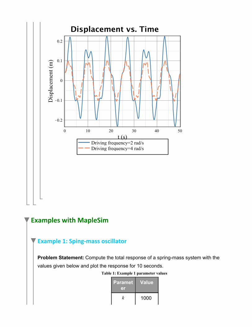
For example, the following plot shows the response of an undamped system with rad/s, m and m/s to harmonic excitation (sine function) of

magnitude N/kg at rad/s and rad/s.

plotplot

Examples with MapleSim

Example 1: Sping-mass oscillator

Problem Statement: Compute the total response of a spring-mass system with the

values given below and plot the response for 10 seconds.Table 1: Example 1 parameter values

Parameter

Value

1000

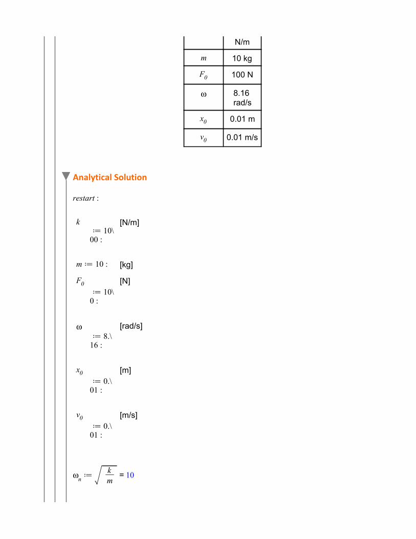
N/m

10 kg

100 N

8.16 rad/s

0.01 m

0.01 m/s

Analytical Solution

[N/m]

[kg]

[N]

[rad/s]

[m]

[m/s]

= 10

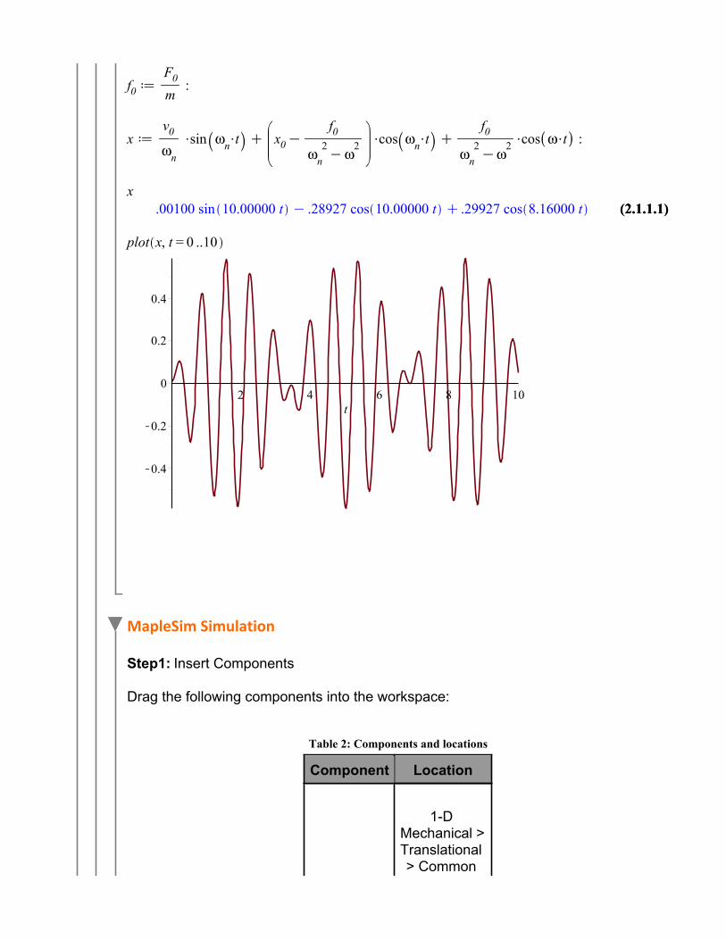
(2.1.1.1)(2.1.1.1)

MapleSim Simulation

Step1: Insert Components

Drag the following components into the workspace:

Table 2: Components and locations

Component Location

1-D Mechanical >Translational > Common

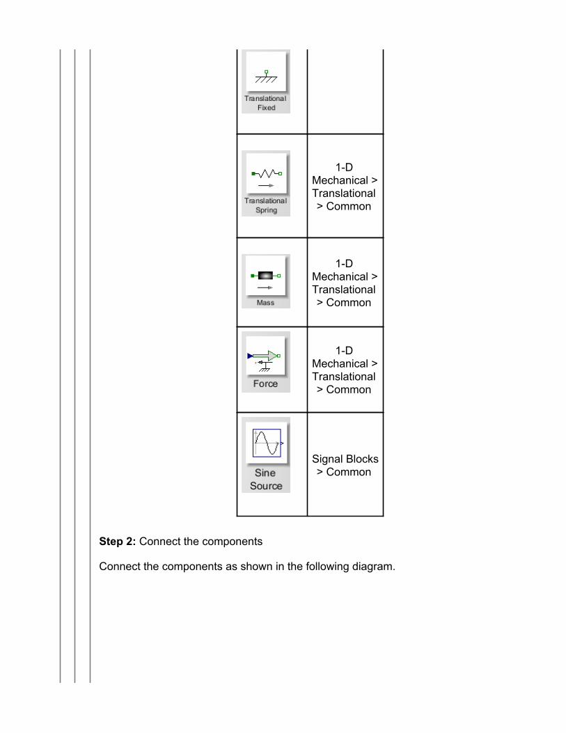
1-D Mechanical >Translational > Common

1-D Mechanical >Translational > Common

1-D Mechanical >Translational > Common

Signal Blocks> Common

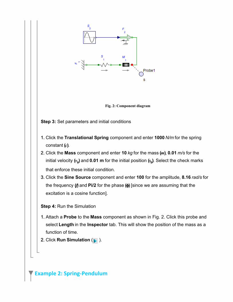
Step 2: Connect the components

Connect the components as shown in the following diagram.

2. 2.

2. 2.

1. 1.

3. 3.

1. 1.

Fig. 2: Component diagram

Step 3: Set parameters and initial conditions

Click the Translational Spring component and enter 1000 N/m for the spring

constant ( ).Click the Mass component and enter 10 kg for the mass ( ), 0.01 m/s for the

initial velocity ( ) and 0.01 m for the initial position ( ). Select the check marks

that enforce these initial condition.

Click the Sine Source component and enter 100 for the amplitude, 8.16 rad/s for

the frequency ( ) and Pi/2 for the phase ( ) [since we are assuming that the

excitation is a cosine function].

Step 4: Run the Simulation

Attach a Probe to the Mass component as shown in Fig. 2. Click this probe and

select Length in the Inspector tab. This will show the position of the mass as a

function of time.

Click Run Simulation ( ).

Example 2: Spring-Pendulum

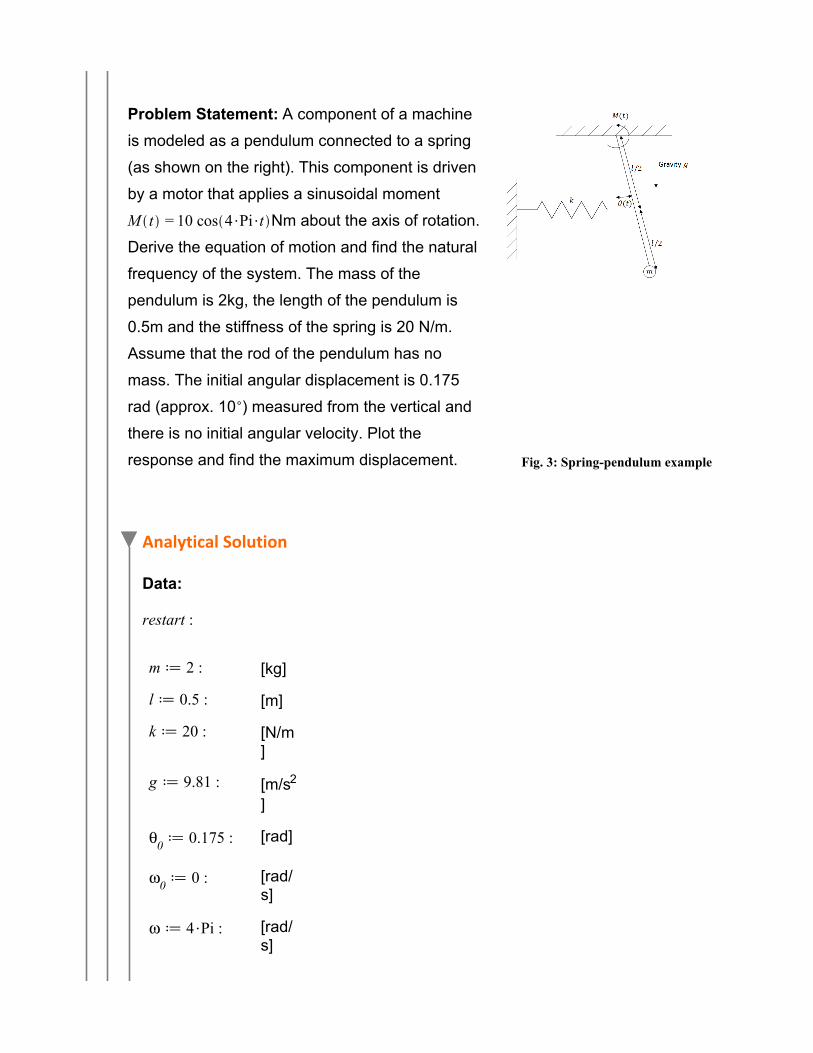
Problem Statement: A component of a machine

is modeled as a pendulum connected to a spring

(as shown on the right). This component is driven

by a motor that applies a sinusoidal moment

Nm about the axis of rotation.

Derive the equation of motion and find the natural

frequency of the system. The mass of the

pendulum is 2kg, the length of the pendulum is

0.5m and the stiffness of the spring is 20 N/m.

Assume that the rod of the pendulum has no

mass. The initial angular displacement is 0.175

rad (approx. 10 ) measured from the vertical and

there is no initial angular velocity. Plot the

response and find the maximum displacement. Fig. 3: Spring-pendulum example

Analytical Solution

Data:

[kg]

[m]

[N/m]

[m/s2

]

[rad]

[rad/s]

[rad/s]

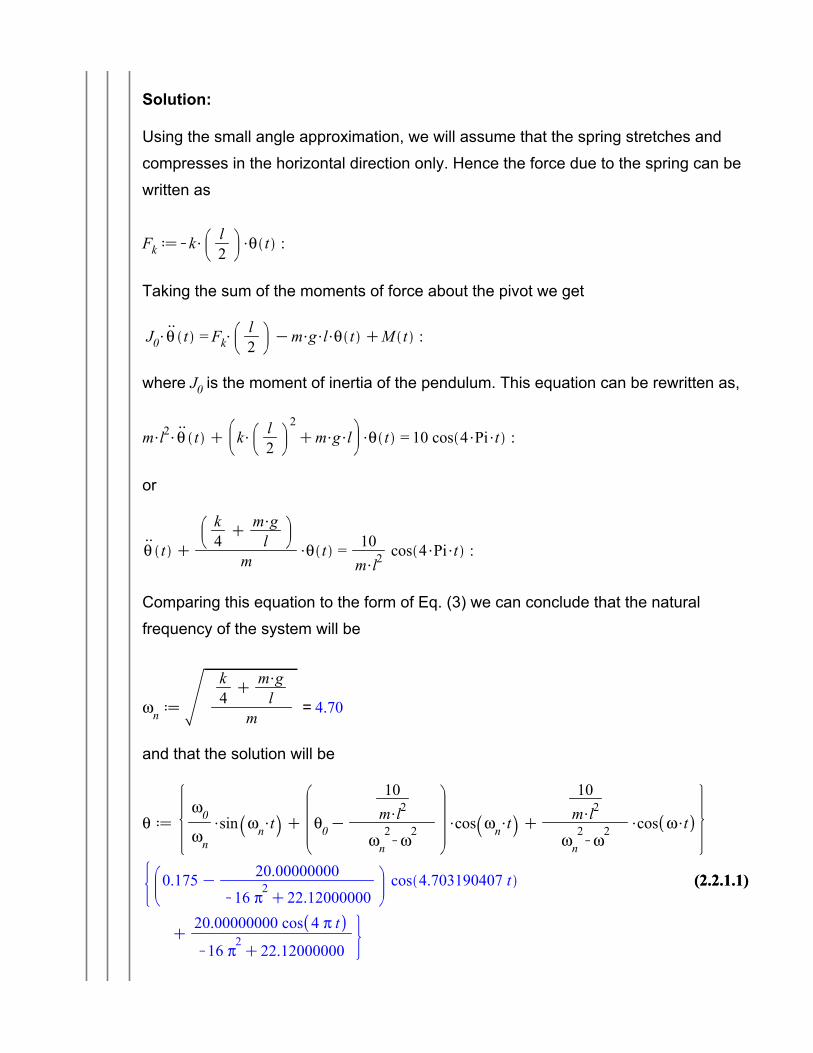
(2.2.1.1)(2.2.1.1)

Solution:

Using the small angle approximation, we will assume that the spring stretches and

compresses in the horizontal direction only. Hence the force due to the spring can be

written as

Taking the sum of the moments of force about the pivot we get

where is the moment of inertia of the pendulum. This equation can be rewritten as,

or

Comparing this equation to the form of Eq. (3) we can conclude that the natural

frequency of the system will be

=

and that the solution will be

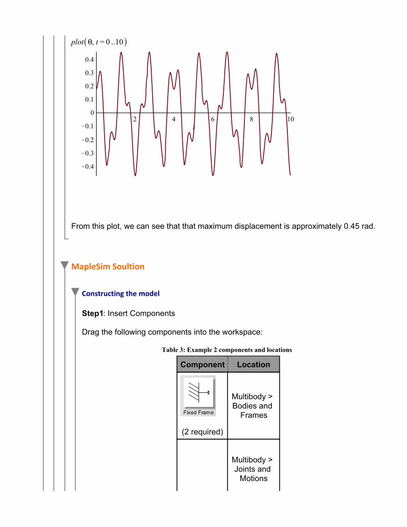
From this plot, we can see that that maximum displacement is approximately 0.45 rad.

MapleSim Soultion

Constructing the model

Step1: Insert Components

Drag the following components into the workspace:

Table 3: Example 2 components and locations

Component Location

(2 required)

Multibody > Bodies and

Frames

Multibody > Joints and

Motions

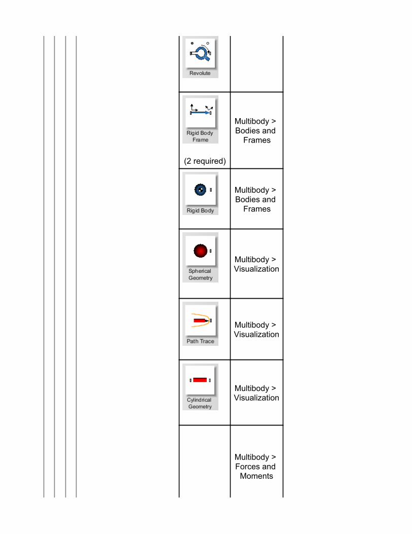
(2 required)

Multibody > Bodies and

Frames

Multibody > Bodies and

Frames

Multibody > Visualization

Multibody > Visualization

Multibody > Visualization

Multibody > Forces and

Moments

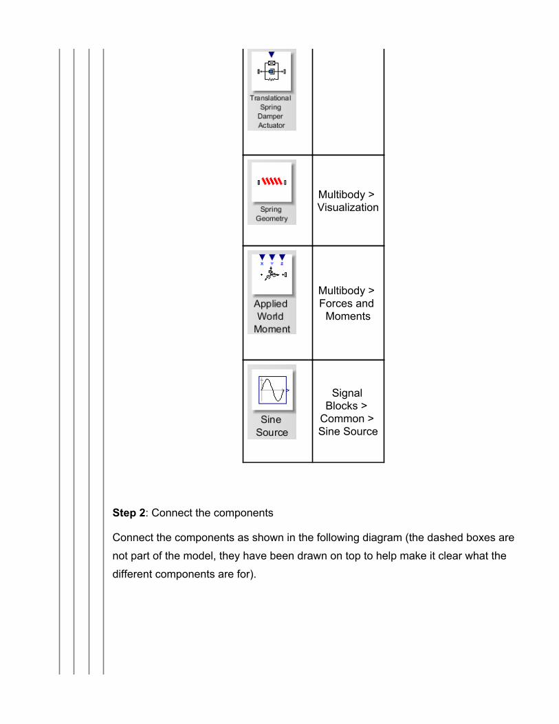
Multibody > Visualization

Multibody > Forces and

Moments

Signal Blocks >

Common > Sine Source

Step 2: Connect the components

Connect the components as shown in the following diagram (the dashed boxes are

not part of the model, they have been drawn on top to help make it clear what the

different components are for).

2. 2.

1. 1.

3. 3.

2. 2.

1. 1.

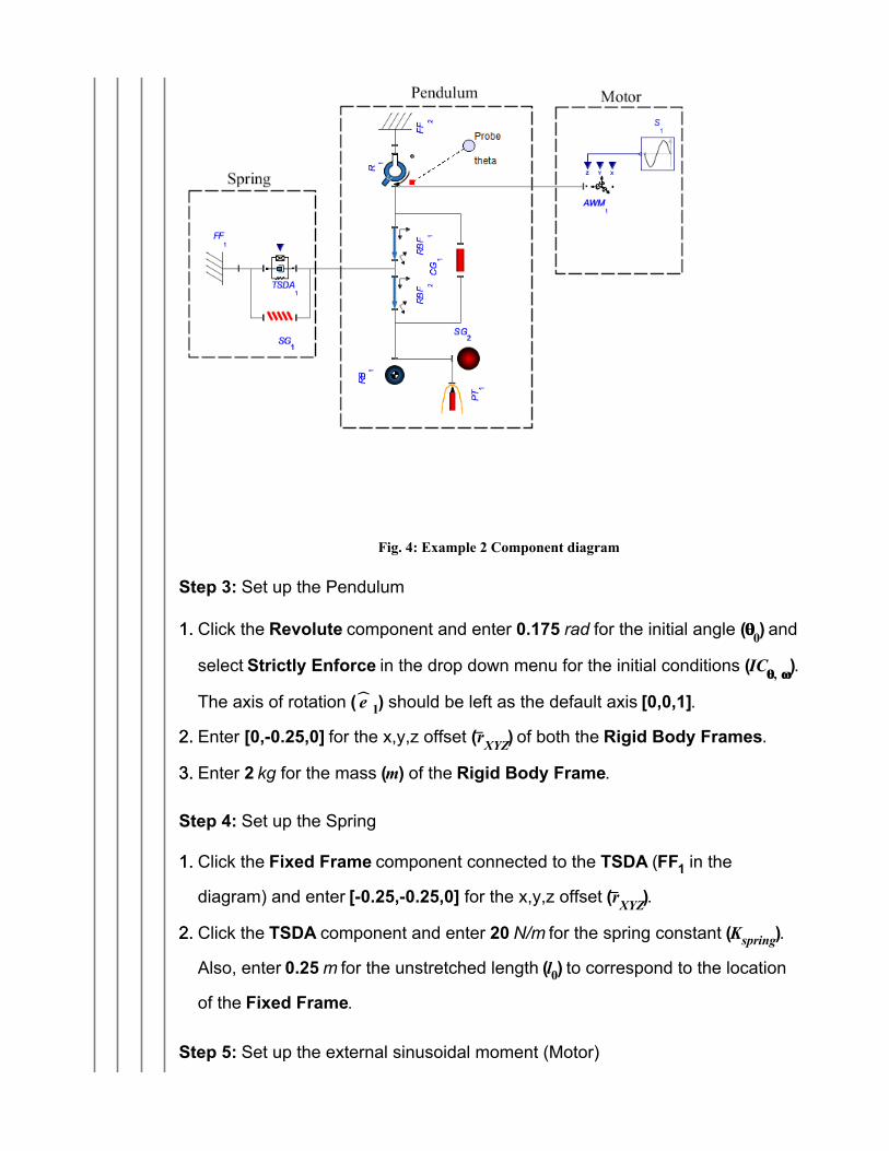
Fig. 4: Example 2 Component diagram

Step 3: Set up the Pendulum

Click the Revolute component and enter 0.175 rad for the initial angle ( ) and

select Strictly Enforce in the drop down menu for the initial conditions ( ).

The axis of rotation ( ) should be left as the default axis [0,0,1].

Enter [0,-0.25,0] for the x,y,z offset ( ) of both the Rigid Body Frames.

Enter 2 kg for the mass ( ) of the Rigid Body Frame.

Step 4: Set up the Spring

Click the Fixed Frame component connected to the TSDA (FF1 in the

diagram) and enter [-0.25,-0.25,0] for the x,y,z offset ( ).

Click the TSDA component and enter 20 N/m for the spring constant ( ).

Also, enter 0.25 m for the unstretched length ( ) to correspond to the location

of the Fixed Frame.

Step 5: Set up the external sinusoidal moment (Motor)

2. 2.

1. 1.

1. 1.

1. 1.

2. 2.

2. 2.

3. 3.

Click the Sine Source component and enter 10 for the amplitude, 4*Pi rad/s

for the frequency ( ) and Pi/2 for the phase ( ) [the external force is a cosine

function].

Connect the output of the Sine Source component to the z input of the Applied World Moment component.

Step 6: Set up the visualization (Inserting the Visualization components is optional)

Click the Cylindrical Geometry component and enter a value around 0.01 m

for the radius.

Click the Spherical Geometry component and enter a value around 0.05 m

for the radius.

Click the Spring Geometry component, enter a number around 10 for the

number of windings, enter a value around 0.02 m for radius1 and enter a

value around 0.005 m for radius2.

Step 7: Run the Simulation

Click the Probe attached to the Revolute joint and select Angle to obtain a

plot of the angular position vs. time.

Click Run Simulation ( ).

Since the analytical solution makes a small angle approximation, there will be a very

slight variation in the results of this simulation and the results of the analytical method.

From the plot generated using the analytical approach, the maximum amplitude is

found to be approximately 0.45 rad. And, from the plot generated using the simulation,

the maximum amplitude is found to be approximately 0.47 rad.

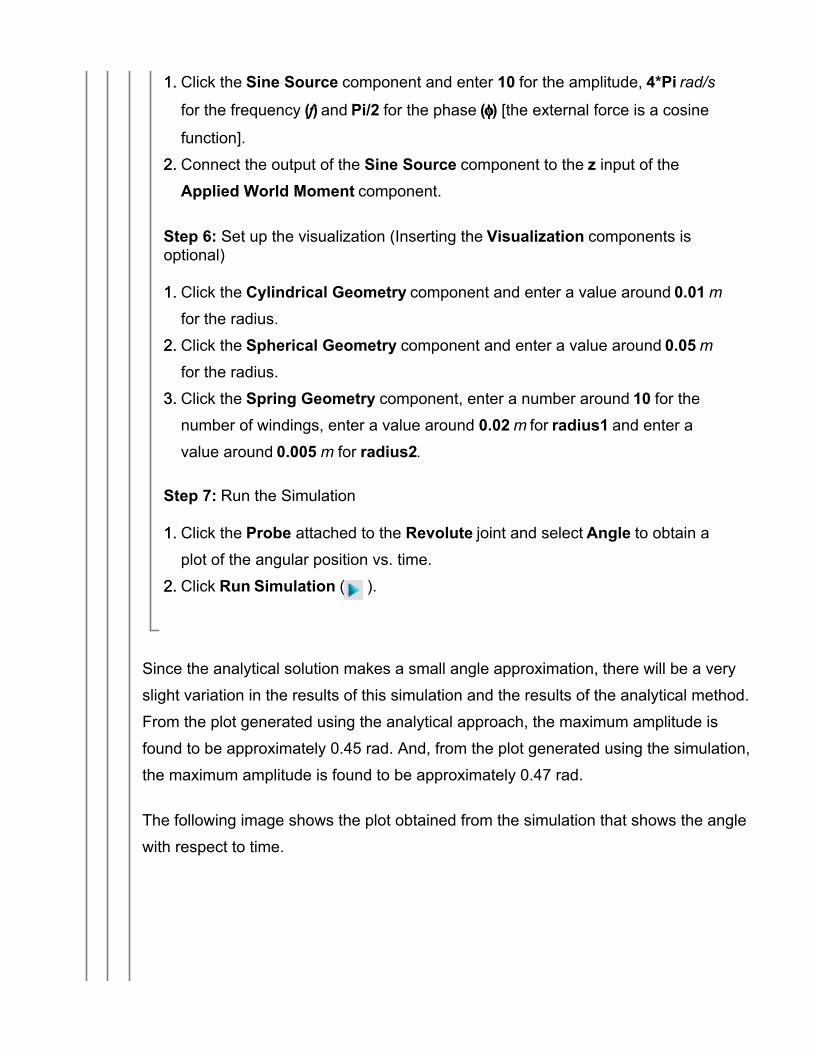
The following image shows the plot obtained from the simulation that shows the angle

with respect to time.

1. 1.

Fig. 5: Simulation results (theta vs. t)

The following video shows the visualization of the simulation

Video Player

Video 1: Visualization of the spring-pendulum simulation

Reference:

D. J. Inman. "Engineering Vibration", 3rd Edition. Upper Saddle River, NJ, 2008, Pearson

Education, Inc.