Download - Forecasting exchange rates using general regression neural networks

Computers & Operations Research 27 (2000) 1093}1110

Forecasting exchange rates using general regression neuralnetworks

Mark T. Leung!,*, An-Sing Chen", Hazem Daouk#

!Division of Management and Marketing, College of Business, University of Texas at San Antonio,San Antonio, TX 78249, USA

"Department of Finance, National Chung Cheng University, Ming Hsiung, Chia Yi 612, Taiwan, ROC#Department of Finance, Kelley School of Business, Indiana University, Bloomington, IN 47405, USA

Abstract

In this study, we examine the forecastability of a speci"c neural network architecture called generalregression neural network (GRNN) and compare its performance with a variety of forecasting techniques,including multi-layered feedforward network (MLFN), multivariate transfer function, and random walkmodels. The comparison with MLFN provides a measure of GRNN's performance relative to the moreconventional type of neural networks while the comparison with transfer function models examines the di!erencein predictive strength between the non-parametric and parametric techniques. The di$cult to beat random walkmodel is used for benchmark comparison. Our "ndings show that GRNN not only has a higher degree offorecasting accuracy but also performs statistically better than other evaluated models for di!erent currencies.

Scope and purpose

Predicting currency movements has always been a problematic task as most conventional econometricmodels are not able to forecast exchange rates with signi"cantly higher accuracy than a naive random walkmodel. For large multinational "rms which conduct substantial currency transfers in the course of business,being able to accurately forecast the movements of exchange rates can result in considerable improvement inthe overall pro"tability of the "rm. In this study, we apply the general regression neural network (GRNN) topredict the monthly exchange rates of three currencies, British pound, Canadian dollar, and Japanese yen.Our empirical experiment shows that the performance of GRNN is better than other neural network andeconometric techniques included in this study. The results demonstrate the predictive strength of GRNN andits potential for solving "nancial forecasting problems. ( 2000 Elsevier Science Ltd. All rights reserved.

Keywords: General regression neural networks; Currency exchange rate; Forecasting

*Corresponding author. Tel.: #1-210-458-5776; fax: #1-210-458-5783.E-mail addresses: [email protected] (M.T. Leung), "[email protected] (A.-S. Chen), [email protected]

(H. Daouk)

0305-0548/00/$ - see front matter ( 2000 Elsevier Science Ltd. All rights reserved.PII: S 0 3 0 5 - 0 5 4 8 ( 9 9 ) 0 0 1 4 4 - 6

1. Introduction

Applying quantitative methods for forecasting in "nancial markets and assisting investmentdecision making has become more indispensable in business practices than ever before. For largemultinational "rms which conduct substantial currency transfers in the course of business, beingable to accurately forecast movements of currency exchange rates can result in substantialimprovement in the overall pro"tability of the "rm. Nevertheless, predicting exchange ratemovements is still a problematic task. Most conventional econometric models are not able toforecast exchange rates with signi"cantly higher accuracy than a naive random walk model. Inrecent years, there has been a growing interest to adopt the state-of-the-art arti"cial intelligencetechnologies to solve the problem. One stream of these advanced techniques focuses on the use ofarti"cial neural networks (ANN) to analyze the historical data and provide predictions to futuremovements in the foreign exchange market. In this study, we apply a special class of neuralnetworks, called general regression neural network (GRNN), to forecast the monthly exchangerates for three internationally traded currencies, Canadian dollar, Japanese yen, and British pound.In order to provide a fair and robust evaluation of the GRNN, relative performance against otherforecasting approaches are included in our empirical investigation. Speci"cally, the performance ofthe GRNN is compared with those of the multi-layered feedforward neural network (MLFN), thetype of ANN used in many research studies, and the models based on multivariate transferfunction, a general econometric forecasting tool. In addition, random walk forecasts are generatedto give benchmark comparisons.

The remainder of this paper is organized as follows. A review of the literature is given in the nextsection. In Section 3, we give an explanation of the logic and operations used by the GRNN. Then,a description of the empirical data employed in our study is provided in Section 4. This section alsoexplains the neural network training paradigm and presents the model speci"cations for theforecasting approaches tested in the experiment. In Section 5, a description to our statistical analysesis presented and the experimental "ndings are discussed. The paper is then concluded in Section 6.

2. Literature review

2.1. Exchange rate forecasting

The theory of exchange rate determination is in an unsatisfactory state. From the theoreticalpoint of view, the debates between the traditional #ow approach and the modern asset-marketapproach have seen the victory of the latter. However, from the empirical point of view, theforecasting ability of the theoretical models remains very poor. The results of Meese and Rogo![1}3] came as a shock to the profession. According to these studies, the current structural modelsof exchange-rate determination failed to outperform the random walk model in out-of-sampleforecasting experiments even when the actual realized values of the explanatory variables were used(ex-post forecasts). The results of Meese and Rogo! have been con"rmed in many subsequentpapers (e.g., Alexander and Thomas [4], Gandolfo et al. [5,6], and Sarantis and Stewart, [7,8]).Moreover, even with the use of sophisticated techniques, such as time-varying-coe$cients, theforecasts are only marginally better that the random walk model [9].

1094 M.T. Leung et al. / Computers & Operations Research 27 (2000) 1093}1110

The models considered by Meese and Rogo! were the #exible-price (Frenkel}Bilson) monetarymodel, the sticky-price (Dornbusch}Frankel) monetary model, and the sticky-price (Hooper}Morton) asset model. Other models for exchange rate forecasting include the portfolio balancemodel, and the uncovered interest parity model. Of the three models used by Meese and Rogo!, theHooper}Morton model is more general and nests the other two models. However, as argued in theprevious paragraph, those three models have been shown to be unsatisfactory. The evidence relatedto the portfolio balance model was ambiguous [7]. On the other hand, both Fisher et al. [10] andSarantis and Stewart [7] found that the models based on a modi"ed uncovered interest parity(MUIP) approach showed some promising results compared to the other conventional theoreticalapproaches. In a related paper, Sarantis and Stewart [8] provided evidence that exchange rateforecasting models based on the MUIP produced more accurate out-of-sample forecasts than theportfolio balance model for all forecast horizons, thus arguing in favor of the MUIP approach toexchange rate determination and forecasting.

In light of the previous literature, we will consider both univariate and multivariate approachesto exchange rate forecasting. Furthermore, given the mounting evidence favoring the MUIPapproach to exchange rate modeling, we use the MUIP relationship as the theoretical basis for ourmultivariate speci"cations in our experimental investigation.

2.2. MUIP exchange rate relationship

Essentially, Sarantis and Stewart [7,8] showed that the MUIP relationship can be modeled andwritten as follows:

et"a

0#a

1(rHt!r

t)#a

2(nH

t!n

t)#a

3(pH

t!p

t)#a

4(ca

t/ny

t)#a

5(caH

t/nyH

t)#k

t, (1)

where e is the natural logarithm of the exchange rate, de"ned as the foreign currency price ofdomestic currency. r,n, p, and (ca/ny) represent the logarithm of nominal short-term interest rate,expected price in#ation rate, the logarithm of the price level, and the ratio of current account tonominal GDP for the domestic economy, respectively. Asterisks denote the corresponding foreignvariables. k is the error term. The variables (ca/ny) and (caH/nyH) are proxies for the risk premium.Eq. (1) is a modi"ed version of the real uncovered interest parity (MUIP) relationship adjusted forrisk. Sarantis and Stewart [7] provided a more detailed discussion and investigation of thisrelationship.

2.3. Applications of neural networks

In the last decade, applications associated with arti"cial neural network (ANN) has been gainingpopularity in both the academic research and practitioner's sectors. The basic structure of andoperations performed by the ANN emulate those found in a biological neural system. Basic notionsof the concepts and principals of the ANN systems and their training procedures can be found inRumelhart and McClelland [11], Lippman [12], and Medsker et al. [13]. Many of the countlessapplications of this arti"cial intelligence technology are related to the "nancial decision making.Hawley et al. [14] provide an overview of the neural network models in the "eld of "nance.

According to Hawley et al., there is a diversity of "nancial applications for neural networks in theareas of corporate "nance, investment analysis, and banking. A review on recent literature also

M.T. Leung et al. / Computers & Operations Research 27 (2000) 1093}1110 1095

reveals "nancial studies on a wide variety of subjects such as bankruptcy prediction [15,16],prediction of savings and loan association failures [17], credit evaluation [18,19], analysis of"nancial statements [20], corporate distress diagnosis [21], bond rating [22], initial stock pricing[23], currency exchange rate forecasting [24], stock market analysis [25}27], and forecasting infutures market [28,29].

2.4. Studies using general regression neural networks

GRNN is a class of neural networks which is capable of performing kernel regression and othernon-parametric functional approximations. Although GRNN has been shown to be a competenttool for solving many scienti"c and engineering problems (e.g., signal processing [30]), chemicalprocessing [31], structural analysis [32], assessment of high power systems [33], the technique hasnot been widely applied to the "eld of "nance and investment. The only one "nancial studyprimarily based on GRNN is Wittkemper and Steiner [34] in which the regression network is usedto verify the predictability of the systematic risk of stocks.

3. General regression neural network

The general regression neural network (GRNN) was originally proposed and developed bySpecht [35]. This class of network paradigm has the distinctive features of learning swiftly, workingwith simple and straightforward training algorithm, and being discriminative against infrequentoutliers and erroneous observations. As its name implies, GRNN is capable of approximating anyarbitrary function from historical data. The foundation of GRNN operation is essentially based onthe theory of nonlinear (kernel) regression* estimation of the expected value of output given a setof inputs. Although GRNN can provide a multivariate vector of outputs, without loss of generality,our description of the GRNN operating logic is simpli"ed to the case of univariate output. Eq. (2)summarizes the GRNN logic in an equivalent nonlinear regression formula:

E[yDX]":=~=

yf (X, y) dy:=~=

f (X, y) dy, (2)

where y is the output predicted by GRNN, X the input vector (x1, x

2,2, x

n) which consists of

n predictor variables, E[yDX] the expected value of the output y given an input vector X, and f (X, y)the joint probability density function of X and y.

3.1. Topology of GRNN

The topology of GRNN developed by Specht [35] primarily consists of four layers of processingunits (i.e., neurons). Each layer of processing units is assigned with a speci"c computationalfunction when nonlinear regression is performed. The "rst layer of processing units, termed inputneurons, are responsible for reception of information. There is a unique input neuron for eachpredictor variable in the input vector X. No processing of data is conducted at the input neurons.The input neurons then present the data to the second layer of processing units called pattern


neurons. A pattern neuron is used to combine and process the data in a systematic fashion suchthat the relationship between the input and the proper response is `memorizeda. Hence, thenumber of pattern neurons is equal to the number of cases in the training set. A typical patternneuron i obtains the data from the input neurons and computes an output h

iusing the transfer

function of

hi"e~(X~Ui ){(X~Ui )@2p2, (3)

where X is the input vector of predictor variables to GRNN, ;i

is the speci"c training vectorrepresented by pattern neuron i, and p is the smoothing parameter.

Eq. (3) is the multivariate Gaussian function extended by Cacoullos [36] and adopted by Spechtin his GRNN design.

The outputs of the pattern neurons are then forwarded to the third layer of processing units,summation neurons, where the outputs from all pattern neurons are augmented. Technically, thereare two types of summations, simple arithmetic summations and weighted summations, performedin the summation neurons. In GRNN topology, there are separate processing units to carry out thesimple arithmetic summations and the weighted summations. Eqs. (4a) and (4b) express themathematical operations performed by the &simple' summation neuron and the &weighted' summa-tion neuron, respectively.

S4"+

i

hi, (4a)

S8"+

i

wihi. (4b)

The sums calculated by the summation neurons are subsequently sent to the fourth layer ofprocessing unit, the output neuron. The output neuron then performs the following division toobtain the GRNN regression output y:

y"S8

S4

. (5)

Fig. 1 illustrates the schematic sketch of the GRNN design and its operational logic describedabove. It should be noted that the depicted network construct is valid for any model withmultivariate outputs. The speci"c design for exchange rate forecasting in our study has only one(univariate) output neuron.

4. Exchange rate forecasting

4.1. Data

The sample data applied to this study are collected from the AREMOS data base maintained bythe Department of Education of Taiwan. The entire data set covers 259 monthly periods runningfrom January 1974 through July 1995. To serve di!erent purposes, the data are divided into threesets: the training set (129 months from January 1974 through September 1984), the model


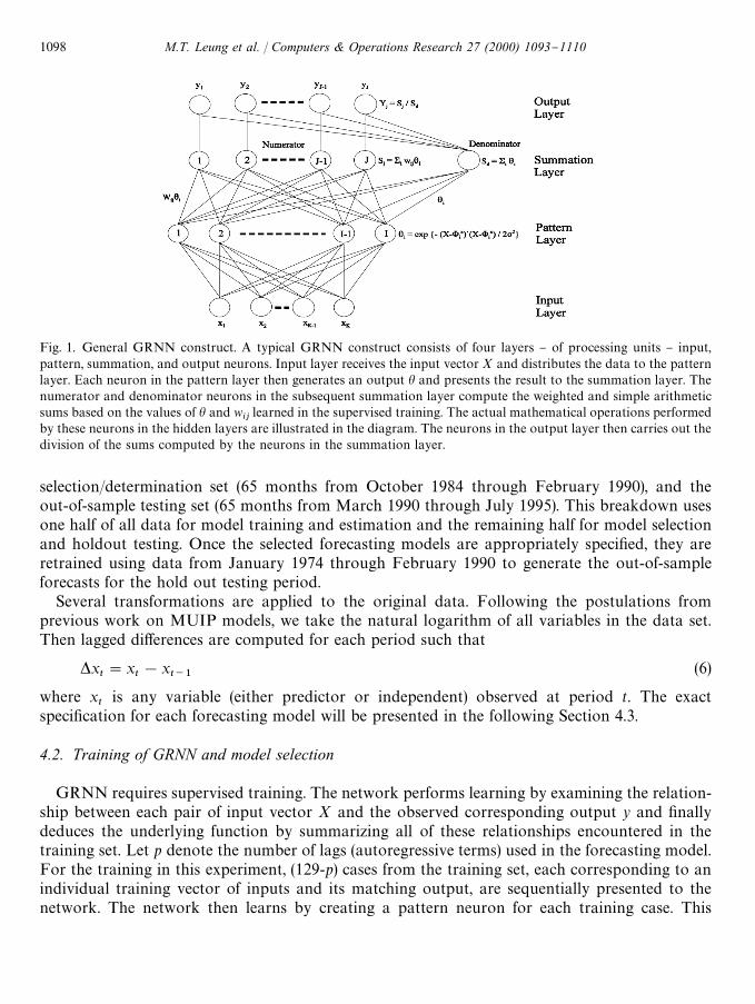
Fig. 1. General GRNN construct. A typical GRNN construct consists of four layers } of processing units } input,pattern, summation, and output neurons. Input layer receives the input vector X and distributes the data to the patternlayer. Each neuron in the pattern layer then generates an output h and presents the result to the summation layer. Thenumerator and denominator neurons in the subsequent summation layer compute the weighted and simple arithmeticsums based on the values of h and w

ijlearned in the supervised training. The actual mathematical operations performed

by these neurons in the hidden layers are illustrated in the diagram. The neurons in the output layer then carries out thedivision of the sums computed by the neurons in the summation layer.

selection/determination set (65 months from October 1984 through February 1990), and theout-of-sample testing set (65 months from March 1990 through July 1995). This breakdown usesone half of all data for model training and estimation and the remaining half for model selectionand holdout testing. Once the selected forecasting models are appropriately speci"ed, they areretrained using data from January 1974 through February 1990 to generate the out-of-sampleforecasts for the hold out testing period.

Several transformations are applied to the original data. Following the postulations fromprevious work on MUIP models, we take the natural logarithm of all variables in the data set.Then lagged di!erences are computed for each period such that

*xt"x

t!x

t~1(6)

where xt

is any variable (either predictor or independent) observed at period t. The exactspeci"cation for each forecasting model will be presented in the following Section 4.3.

4.2. Training of GRNN and model selection

GRNN requires supervised training. The network performs learning by examining the relation-ship between each pair of input vector X and the observed corresponding output y and "nallydeduces the underlying function by summarizing all of these relationships encountered in thetraining set. Let p denote the number of lags (autoregressive terms) used in the forecasting model.For the training in this experiment, (129-p) cases from the training set, each corresponding to anindividual training vector of inputs and its matching output, are sequentially presented to thenetwork. The network then learns by creating a pattern neuron for each training case. This


Fig. 2. GRNN construct for exchange rate forecasting. The design of the illustrated GRNN construct is based on theModi"ed Uncovered Interest Parity (MUIP) theorem. The depicted construct shows in input vector with six groups ofinput variables. Each group of variables contains a "nite number of lagged terms in which the total number of lags di!ersfrom group to group and from one currency to another. There are (129-p) neurons in the pattern layer, representing thetraining cases in the training data set. The value of p is equal to the number of lagged terms in the model speci"cation.After the supervised training is completed, the regression network will compute the exchange rate forecast of periodt based on the values of the predictor variables.

procedure is repeated until all cases in the training set are gone through. Fig. 2 illustrates theGRNN construct after training with (129-p) cases in the training set.

Prediction of the exchange rate forecasts for the model selection/determination period beginsafter the network is trained. The 65 in-sample forecasts are then compared with the actualobservations and the network parameters are adjusted. Afterward, the best three model speci"ca-tions in terms of root mean square error (RMSE) are chosen. The network is then trained using thecases in both training and model selection sets. Estimation of the exchange rates in the holdouttesting period is then performed and performance statistics for these 65 out-of-sample forecasts arecomputed. The entire experimental procedure is repeated for di!erent currencies.

4.3. Forecasting models

In addition to GRNN, a number of di!erent speci"cations (models) based on MLFN (a.k.abackpropagation network), and multivariate transfer function are examined in our experiment.MLFN, a type of neural network architecture widely used in research studies, should providea parallel comparison to GRNN in the area of non-parametric neural network forecasting. On theother hand, multivariate transfer function represents the parametric counterpart of the moreconventional econometric forecasting. Interested readers should refer to Wasserman [37] fora detailed description of MLFN. Also, Markradis et al. [38] provide a good discussion of thefundamentals of multivariate transfer function and a brief summary of this forecasting approachcan be found in the Appendix.


In order to obtain a fair and more robust comparison of GRNN's performance with the others,we pick up the best three speci"cations from each forecasting approach. Like the one for GRNN,the selection criterion is root mean square error (RMSE); however, an alternative criterion of meanabsolute error (MAE) also leads to the same selection. In addition, a random walk model isincluded for benchmark comparisons. After the speci"cations are chosen and the parameters aredetermined, the out-of-sample forecasts from each of these forecasting speci"cations are generatedand subject to statistical evaluations. Hence, our "nal statistical testings involve a total of 10di!erent forecasting models for each currency.

Let F(f) and G(f) denote the implied functional relationships estimated by GRNN and MLFN,respectively. Table 1 show the selected speci"cations for Canadian dollar, Japanese yen, and Britishpound forecasting, respectively. These selected speci"cations are chosen from the best three modelsfrom each of the GRNN, MLFN, and multivariate transfer function approaches. AppendixA contains a detailed description of the notation for representing the transfer function model.

5. Performance evaluation

5.1. Primary statistical evaluation

Five primary statistical measures are computed from the out-of-sample forecasts made by eachselected speci"cation. As described in the previous section, each series of forecasts is checkedagainst with the 65 observed cases in the holdout testing set. The "ve evaluation criteria are: meanabsolute error (MAE), root mean square error (RMSE), ; statistic, and the bias (a) and regressionproportion coe$cient (b) from the Theil's Decomposition Test [39]. The ; statistic is the ratio ofthe RMSE of a model's forecasts to the RMSE of the random walk forecasts of no change in thedependent variable. Since the random walk forecast of next month's exchange rate is equal tothe current month's rate, a ; statistic of less than 1 implies that the tested model outperforms therandom walk model during the holdout period. Likewise, a; statistic in excess of 1 implies that themodel performs worse than the random walk model. The ; statistic has a major advantage overthe RMSE in the comparison of forecasting models because it is a unit-free measurement. Thus, it iseasier to calibrate the relative performances by ; statistic than by the unit-bound RMSE.

The Theil's Decomposition Test [39] is conducted by regressing the actual observed exchangerates on a constant and the predicted exchange rates e(

testimated by a particular model.

et"a#be(

t. (7)

The constant a (bias coe$cient) should be insigni"cantly di!erent from zero and the coe$cientb for predicted exchange rate variable (regression proportion coe$cient) should be insigni"cantlydi!erent from one for the forecast to be acceptable.

Table 2 summarizes the performance statistics based on the 65 out-of-sample forecasts (fromMarch 1990 through July 1995) generated by the GRNN, MLFN, multivariate transfer functionand random walk models. Results in Table 2 illustrate that the GRNN models generally outper-form the parametric multivariate transfer function and the random walk models. In addition, theGRNN models generates more accurate forecasts than MLFN, its neural network counterpart.


Table 1

(a) The selected model speci"cations for Canadian dollar forecasting in the holdout testing period. The three modelspeci"cations yielding the best RMSE in the model selection/determination period are chosen. These models will beevaluated using the data in the holdout testing set (from March 1990 through July 1995). A brief interpretation of thetransfer function modeling and its notation can be found in Appendix A and Markradis et al. [38] provide a furtherdiscussion of this forecasting technique

GRNN Speci"cation 1: AR(1)

*et"F(*e

t~1)


*et"F(*e

t~1,2, *e

t~12)

GRNN Speci"cation 3: AR(1)-MUIP(1)

*et"F(*e

t~1, *(rH!r)

t~1, *(nH!n)

t~1, *(pH!p)

t~1, *(ca/ny)

t~1, *(caH/nyH)

t~1)

MLFN Speci"cation 1: AR(4)

*et"G(*e

t~1,2, *e

t~4)


*et"G(*e

t~1,2, *e

t~5)

MLFN Speci"cation 3: AR(1)-MUIP(1)

*et"G(*e

t~1, *(rH!r)

t~1, *(nH!n)

t~1, *(pH!p)

t~1, *(ca/ny)

t~1, *(caH/nyH)

t~1)

Transfer Function Speci"cation 1: MUIP(0/1)

*et"

u10

(1!d11

¸)*(rH!r)

t~1#

u20

(1!d21

¸)*(nH!n)

t~1#2

Transfer Function Speci"cation 2: ARIMA(1, 0, 0)-MUIP(1/1)

*et"a

0#a

1*e

t~1#

(u10

#u11

¸)

(1!d11

¸)*(rH!r)

t~1#

(u20

#u21

¸)

(1!d21

¸)*(nH!n)

t~1#2


*et"e

t#b

1et~1

#b2et~2

#

u10

(1!d11

¸)*(rH!r)

t~1#

u20

(1!d21

¸)*(nH!n)

t~1#2

(b) The selected model speci"cations for Japanese yen forecasting in the holdout testing period. The three modelspeci"cations yielding the best RMSE in the model selection/determination period are chosen. These models will beevaluated using the data in the holdout testing set (from March 1990 through July 1995). A brief interpretation of thetransfer function modeling and its notation can be found in Appendix A and Markradis et al. [38] provide a furtherdiscussion of this forecasting technique


*et"F(*e

t~1)


*et"F(*e

t~1, *e

t~2)


Table 1 (continued)


*et"F(*e

t~1,2, *e

t~12)


*et"G(*e

t~1, *e

t~2, *e

t~3)


*et"G(*e

t~1,2, *e

t~4)


*et"G(*e

t~1, *(rH!r)

t~1, *(nH!n)

t~1, *(pH!p)

t~1, *(ca/ny)

t~1, *(caH/nyH)

t~1)


*et"a

0#a

1*e

t~1#(u

10#u

11¸)*(rH!r)

t~1#(u

20#u

21¸)*(nH!n)

t~1#2


*et"e

t#b

1et~1

#b2et~2

#

(u10

)

(1!d11

¸)*(rH!r)

t~1#

(u20

)

(1!d21

¸)*(nH!n)

t~1#2


*et"e

t#b

1et~1

#b2et~2

#(u10

#u11

¸)*(rH!r)t~1

#(u20

#u21

¸)*(nH!n)t~1

#2

(c) The selected model speci"cations for British pound forecasting in the holdout testing period. The three modelspeci"cations yielding the best RMSE in the model selection/determination period are chosen. These models will beevaluated using the data in the holdout testing set (from March 1990 through July 1995). A brief interpretation of thetransfer function modeling and its notation can be found in Appendix A and Markradis et al. [38] provide a furtherdiscussion of this forecasting technique


*et"F(*e

t~1)


*et"F(*e

t~1, *e

t~2)

GRNN Speci"cation 3: AR(3)-MUIP(1)

*et"F(*e

t~1, *e

t~2, *e

t~3, *(rH!r)

t~1, *(nH!n)

t~1, *(pH!p)

t~1, *(ca/ny)

t~1, *(caH/nyH)

t~1)


*et"G(*e

t~1, *e

t~2)


*et"G(*e

t~1, *e

t~2, *e

t~3)


*et"G(*e

t~1, *(rH!r)

t~1, *(nH!n)

t~1, *(pH!p)

t~1, *(ca/ny)

t~1, *(caH/nyH)

t~1)


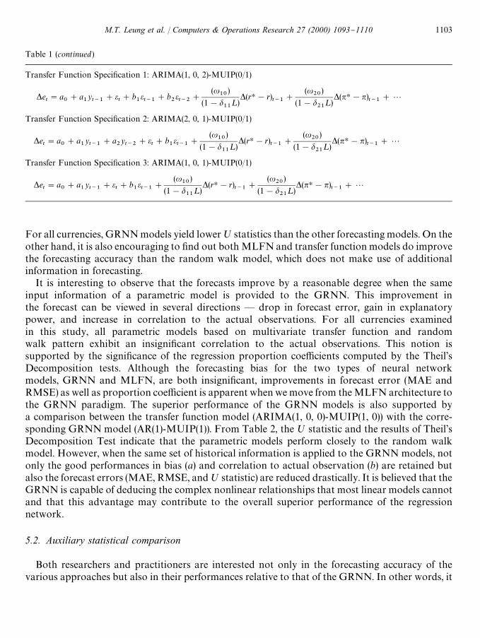
Table 1 (continued)


*et"a

0#a

1yt~1

#et#b

1et~1

#b2et~2

#

(u10

)

(1!d11

¸)*(rH!r)

t~1#

(u20

)

(1!d21

¸)*(nH!n)

t~1#2


*et"a

0#a

1yt~1

#a2yt~2

#et#b

1et~1

#

(u10

)

(1!d11

¸)*(rH!r)

t~1#

(u20

)

(1!d21

¸)*(nH!n)

t~1#2


*et"a

0#a

1yt~1

#et#b

1et~1

#

(u10

)

(1!d11

¸)*(rH!r)

t~1#

(u20

)

(1!d21

¸)*(nH!n)

t~1#2

For all currencies, GRNN models yield lower; statistics than the other forecasting models. On theother hand, it is also encouraging to "nd out both MLFN and transfer function models do improvethe forecasting accuracy than the random walk model, which does not make use of additionalinformation in forecasting.

It is interesting to observe that the forecasts improve by a reasonable degree when the sameinput information of a parametric model is provided to the GRNN. This improvement inthe forecast can be viewed in several directions * drop in forecast error, gain in explanatorypower, and increase in correlation to the actual observations. For all currencies examinedin this study, all parametric models based on multivariate transfer function and randomwalk pattern exhibit an insigni"cant correlation to the actual observations. This notion issupported by the signi"cance of the regression proportion coe$cients computed by the Theil'sDecomposition tests. Although the forecasting bias for the two types of neural networkmodels, GRNN and MLFN, are both insigni"cant, improvements in forecast error (MAE andRMSE) as well as proportion coe$cient is apparent when we move from the MLFN architecture tothe GRNN paradigm. The superior performance of the GRNN models is also supported bya comparison between the transfer function model (ARIMA(1, 0, 0)-MUIP(1, 0)) with the corre-sponding GRNN model (AR(1)-MUIP(1)). From Table 2, the ; statistic and the results of Theil'sDecomposition Test indicate that the parametric models perform closely to the random walkmodel. However, when the same set of historical information is applied to the GRNN models, notonly the good performances in bias (a) and correlation to actual observation (b) are retained butalso the forecast errors (MAE, RMSE, and; statistic) are reduced drastically. It is believed that theGRNN is capable of deducing the complex nonlinear relationships that most linear models cannotand that this advantage may contribute to the overall superior performance of the regressionnetwork.

5.2. Auxiliary statistical comparison

Both researchers and practitioners are interested not only in the forecasting accuracy of thevarious approaches but also in their performances relative to that of the GRNN. In other words, it


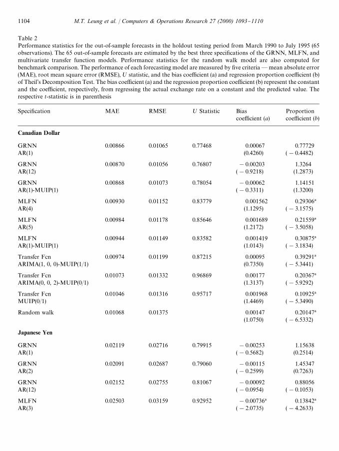
Table 2Performance statistics for the out-of-sample forecasts in the holdout testing period from March 1990 to July 1995 (65observations). The 65 out-of-sample forecasts are estimated by the best three speci"cations of the GRNN, MLFN, andmultivariate transfer function models. Performance statistics for the random walk model are also computed forbenchmark comparison. The performance of each forecasting model are measured by "ve criteria*mean absolute error(MAE), root mean square error (RMSE), ; statistic, and the bias coe$cient (a) and regression proportion coe$cient (b)of Theil's Decomposition Test. The bias coe$cient (a) and the regression proportion coe$cient (b) represent the constantand the coe$cient, respectively, from regressing the actual exchange rate on a constant and the predicted value. Therespective t-statistic is in parenthesis

Speci"cation MAE RMSE ; Statistic Bias Proportioncoe$cient (a) coe$cient (b)

Canadian Dollar

GRNN 0.00866 0.01065 0.77468 0.00067 0.77729AR(1) (0.4260) (!0.4482)

GRNN 0.00870 0.01056 0.76807 !0.00203 1.3264AR(12) (!0.9218) (1.2873)

GRNN 0.00868 0.01073 0.78054 !0.00062 1.14151AR(1)-MUIP(1) (!0.3311) (1.3200)

MLFN 0.00930 0.01152 0.83779 0.001562 0.29306!AR(4) (1.1295) (!3.1575)

MLFN 0.00984 0.01178 0.85646 0.001689 0.21559!AR(5) (1.2172) (!3.5058)

MLFN 0.00944 0.01149 0.83582 0.001419 0.30875!AR(1)-MUIP(1) (1.0143) (!3.1834)

Transfer Fcn 0.00974 0.01199 0.87215 0.00095 0.39291!ARIMA(1, 0, 0)-MUIP(1/1) (0.7350) (!5.3441)

Transfer Fcn 0.01073 0.01332 0.96869 0.00177 0.20367!ARIMA(0, 0, 2)-MUIP(0/1) (1.3137) (!5.9292)

Transfer Fcn 0.01046 0.01316 0.95717 0.001968 0.10925!MUIP(0/1) (1.4469) (!5.3490)

Random walk 0.01068 0.01375 0.00147 0.20147!(1.0750) (!6.5332)

Japanese Yen

GRNN 0.02119 0.02716 0.79915 !0.00253 1.15638AR(1) (!0.5682) (0.2514)

GRNN 0.02091 0.02687 0.79060 !0.00115 1.45347AR(2) (!0.2599) (0.7263)

GRNN 0.02152 0.02755 0.81067 !0.00092 0.88056AR(12) (!0.0954) (!0.1053)

MLFN 0.02503 0.03159 0.92952 !0.00736! 0.13842!

AR(3) (!2.0735) (!4.2633)


Table 2 (continued)

Speci"cation MAE RMSE ; Statistic Bias Proportioncoe$cient (a) coe$cient (b)

MLFN 0.02480 0.03129 0.92063 !0.00596 0.24263!

AR(4) (!1.6240) (!4.4870)

MLFN 0.02585 0.03264 0.96043 !0.00728! 0.17606!

AR(1)-MUIP(1) (!2.0811) (!4.9401)

Transfer Fcn 0.02305 0.02925 0.86076 !0.00651 0.15776!ARIMA(1, 0, 0)-MUIP(1/0) (!1.4983) (!2.7612)

Transfer Fcn 0.02476 0.03071 0.90366 !0.00684 0.17317!

ARIMA(0, 0, 2)-MUIP(0/1) (!1.8520) (!3.8799)


Random walk 0.02667 0.03398 !0.00588 0.23853!(!1.6584) (!6.1236)

British Pound

GRNN 0.02212 0.02865 0.83143 !0.00023 1.37134AR(1) (!0.0645) (0.8022)

GRNN 0.02202 0.02855 0.82852 !0.00014 1.38586AR(2) (!0.0398) (0.8526)

GRNN 0.02161 0.02995 0.86893 0.00105 1.73073AR(3)-MUIP(1) (0.2788) (1.6130)

MLFN 0.02309 0.02996 0.86932 0.00092 0.59779AR(2) (0.2474) (!1.3206)

MLFN 0.02468 0.03119 0.90504 0.00167 0.41215!AR(3) (0.4422) (!2.3484)

MLFN 0.02216 0.02990 0.86757 0.00437 0.65691AR(1)-MUIP(1) (1.1354) (!1.4107)




Random walk 0.02706 0.03446 0.00075 0.36029!(0.21139) (!5.4774)

!Indicates signi"cance at 5% level for H0: a"0 and H

0: b"1.


Table 3Pairwise t-tests for the di!erence in forecasting accuracy between GRNN and other forecasting approaches. Thet-statistics are based on comparisons of the MAE and RMSE of the GRNN forecasts in the holdout testing period (fromMarch 1990 to July 1995) with those of the MLFN, multivariate transfer function, and random walk models. The bestthree speci"cations from each forecasting approach provide a total 3]65"195 matching observations for each t-test.The null hypothesis is no di!erence in the forecasting accuracy between GRNN and the tested approach

MAE RMSE

t-statistic p value t-statistic p value

Canadian dollarMLFN 2.3543! 0.0195 2.3178! 0.0215Transfer function 2.8192 0.0053 3.0259 0.0028Random walk 3.7160 0.0003 5.0664 7.87]10~7

Japanese YenMLFN 3.8208! 0.0002 4.0384! 7.77]10~5

Transfer function 3.7393! 0.0002 3.3474! 0.0010Random walk 3.6447! 0.0003 3.5303! 0.0005

British PoundMLFN 1.6192 0.1071 1.4350 0.1529Transfer function 1.7231" 0.0865 1.7344" 0.0845Random walk 3.6214 0.0004 2.6995! 0.0076

!Signi"cance at the 5% level."Signi"cance at the 10% level.

is important to "nd out whether GRNN forecasting signi"cantly outperforms the others. Giventhis notion, we perform a series of t-tests to determine the signi"cance of the di!erences of meanswith respect to the MAE and RMSE measures.

Table 3 reports the results of the conducted pairwise t-tests. For Canadian dollar and Japaneseyen, all comparisons are found to be signi"cant at a"0.05 level, suggesting that GRNN fore-casts are statistically better than the forecasts made by MLFN, multivariate transfer function,and random walk models. These results are also consistent with the "ndings in the previoussection. However, the conclusions are di!erent in the case of British pound forecasting. Asindicated in Table 3, the GRNN forecasts yield lower forecast errors than the random walk modelat a"0.05 level. Nevertheless, the signi"cance in the di!erence is reduced to a"0.10 level whenGRNN forecasts are compared with those estimated by the transfer function models. For thecomparison with MLFN, the quality of the two neural network approaches are statisticallyindi!erent, showing that the more conventional MLFN is still a valuable tool in forecastingresearch.

The disparity in the ranking of the comparison tests here suggests some interesting points. First,although the forecasting accuracy in terms of MAE and RMSE are quite similar between MLFNand GRNN, a comparison of their ; statistics, which is a relative improvement measure to therandom walk model, indicates the existence of a gap in their performances. This belief is further


supported by the (regression proportion coe$cients) results of Theil's Decomposition test in thatthe GRNN forecasts closely follow the actual exchange rate movements but the MLFN pre-diction has some di$culty to match with the reality. The implication to the researchers is thata more comprehensive framework of evaluation has to be developed and misleading conclusionsmay be drawn if the study relies upon only a couple of conventional statistics (e.g., RMSE,R-square).

Second, as we have expected, the experiment illustrates a varying degree of predictability ofdi!erent currencies. For example, based on the values of RMSE and ; statistics, we can observethat, to a certain extent, the movement of Canadian dollar is more predictable than the othertwo currencies. Japanese yen is the worst among the three examined currencies. This maybe explained by the more volatile economy in Asia than in North America. A closerexamination of the MAE and RMSE across di!erent currencies substantiates the notionthat the Japanese and British currencies have undergone wider #uctuations in their history.The closer performance of GRNN, MLFN, and multivariate transfer function in British poundsuggests the possibility of developing a hybrid forecasting approach in these hard-to-predictenvironments. The hybrid framework may utilize di!erent neural network architectures or evena mix of learning network and parametric technique. In this case, it is hoped that the simultaneoususe of neural network and parametric technique may add predictive strength to the combinednetwork.

6. Conclusions

This exploratory research examines the potential of using GRNN to predict the foreign currencyexchange rates. Empirical results suggest that this nonparametric regression neural network mayprovide better forecasts than the other forecasting approaches tested in this study. This isillustrated by a comparison of the forecasting quality of the GRNN with that of the MLFN,a neural network architecture widely used in the literature, and multivariate transfer function, alsoanother general parametric technique in econometric analyses. The comparative evaluation isbased on a variety of statistics which measure di!erent forms of forecast errors. For all currenciesincluded in our empirical investigation, GRNN models outperform the models associated withMLFN, multivariate transfer function, and random walk. Moreover, our analysis "nds that, exceptthe case of British pound, the means of MAE and RMSE for the GRNN forecasts are signi"cantlylower than those of other approaches. In the future, it would be interesting and bene"cial to verifythe predictive strength of GRNN on other "nancial assets, especially on the relative basis ofMLFN.

Acknowledgements

The authors are grateful for the helpful comments from the two anonymous referees andJatinder Gupta, the guest editor of this special issue. The authors would also like tothank M. Nimalendran and the participants at the 1999 Financial Management AssociationMeeting.


Appendix A

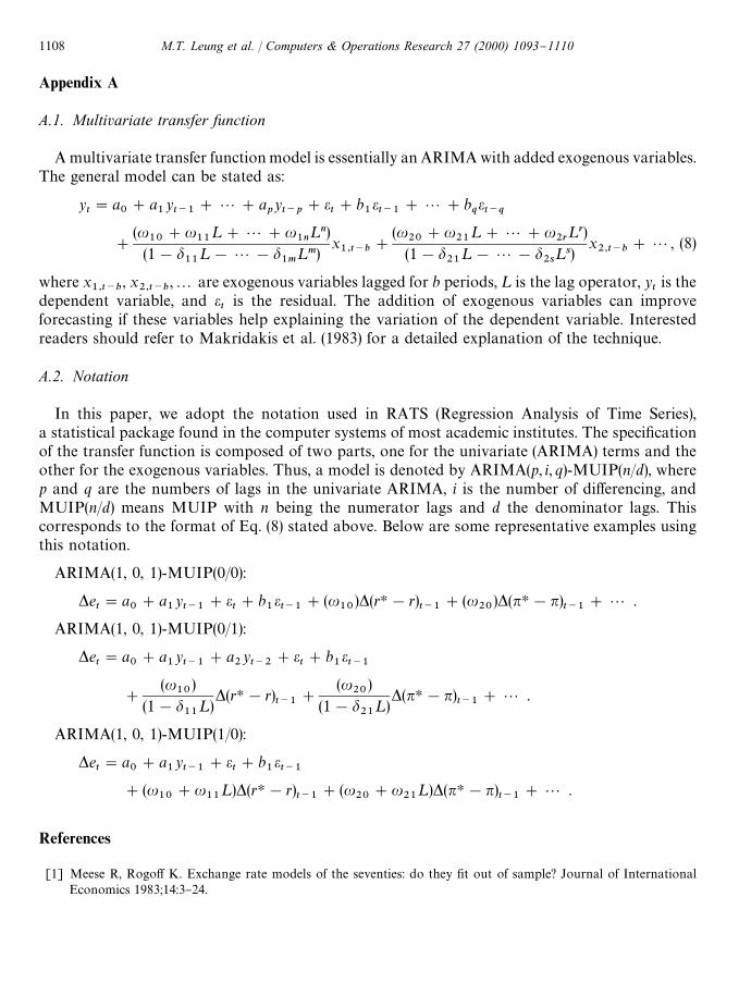
A.1. Multivariate transfer function

A multivariate transfer function model is essentially an ARIMA with added exogenous variables.The general model can be stated as:

yt"a

0#a

1yt~1

#2#apyt~p

#et#b

1et~1

#2#bqet~q

#

(u10

#u11

¸#2#u1n¸n)

(1!d11

¸!2!d1m

¸m)x1,t~b

#

(u20

#u21

¸#2#u2r¸r)

(1!d21

¸!2!d2s¸s)

x2,t~b

#2, (8)

where x1,t~b

, x2,t~b

,2 are exogenous variables lagged for b periods, ¸ is the lag operator, ytis the

dependent variable, and et

is the residual. The addition of exogenous variables can improveforecasting if these variables help explaining the variation of the dependent variable. Interestedreaders should refer to Makridakis et al. (1983) for a detailed explanation of the technique.

A.2. Notation

In this paper, we adopt the notation used in RATS (Regression Analysis of Time Series),a statistical package found in the computer systems of most academic institutes. The speci"cationof the transfer function is composed of two parts, one for the univariate (ARIMA) terms and theother for the exogenous variables. Thus, a model is denoted by ARIMA(p, i, q)-MUIP(n/d), wherep and q are the numbers of lags in the univariate ARIMA, i is the number of di!erencing, andMUIP(n/d) means MUIP with n being the numerator lags and d the denominator lags. Thiscorresponds to the format of Eq. (8) stated above. Below are some representative examples usingthis notation.

ARIMA(1, 0, 1)-MUIP(0/0):

*et"a

0#a

1yt~1

#et#b

1et~1

#(u10

)*(rH!r)t~1

#(u20

)*(nH!n)t~1

#2 .

ARIMA(1, 0, 1)-MUIP(0/1):

*et"a

0#a

1yt~1

#a2yt~2

#et#b

1et~1

#

(u10

)(1!d

11¸)

*(rH!r)t~1

#

(u20

)(1!d

21¸)

*(nH!n)t~1

#2 .

ARIMA(1, 0, 1)-MUIP(1/0):

*et"a

0#a

1yt~1

#et#b

1et~1

#(u10

#u11

¸)*(rH!r)t~1

#(u20

#u21

¸)*(nH!n)t~1

#2 .

References

[1] Meese R, Rogo! K. Exchange rate models of the seventies: do they "t out of sample? Journal of InternationalEconomics 1983;14:3}24.


[2] Meese R, Rogo! K. The out-of-sample failure of empirical exchange rate models: sampling error or misspeci"ca-tion? In: Frenkel J, editor. Exchange rates and international macroeconomics, Chicago University of Chicago Press1983.

[3] Meese R, Rogo!K. Was it real? The exchange rate-interest di!erential relation in 1973}1974. International "nancediscussion paper no. 268, Federal Reserve Board, Washington, DC, 1985.

[4] Alexander D, Thomas LR. Monetary/Asset models of exchange rate determination: how well have they performedin the 1980's?. International Journal of Forecasting 1987;3:53}64.

[5] Gandolfo G, Padoan PC, Paladino G. Structural models versus random walk: the case of the lira/$ exchange rate.Eastern Economic Journal 1990;16:101}13.

[6] Gandolfo G, Padoan PC, Paladino G. Exchange rate determination: single equation or economy-wide models?A test against the random walk. Journal of Banking and Finance 1990;14:965}92.

[7] Sarantis N, Stewart C. Monetary and asset market models for sterling exchange rates: a cointegration approach.Journal of Economic Integration 1995;10:335}71.

[8] Sarantis N, Stewart C. Structural, VAR and BVAR models of exchange rate determination: a comparison of theirforecasting performance. Journal of Forecasting 1995;14:201}15.

[9] Schinasi GJ, Swamy PA. The out-of-sample forecasting performance of exchange rate models when coe$cients areallowed to change. Journal of International Money and Finance 1989;8:373}90.

[10] Fisher PG, Tunna SK, Turner DS, Wallis KF, Whitley JD. Econometric evaluation of the exchange rate models ofthe U.K. economy. Economic Journal 1990;100:1230}44.

[11] Rumelhart D, McClelland J. Parallel distributed processing. Cambridge, MA: MIT Press, 1986.[12] Lippman R. An introduction to computing with neural nets. IEEE ASSP Magazine, 1987:4}22.[13] Medsker L, Turban E, Trippi R. Neural network fundamentals for "nancial analysts. In: Trippi R, Turban E,

editors. Neural networks in "nance and investing. Chicago: Probus Publishing, 1993.[14] Hawley D, Johnson J, Raina D. Arti"cial neural systems: a new tool for "nancial decision-making. Financial

Analysts Journal 1990:63}72.[15] Tsukuda J, Baba S. Predicting Japanese corporate bankruptcy in terms of "nancial data using a neural network.

Computers and Industrial Engineering 1994;27:445}8.[16] Tam KY, Kiang MY. Managerial applications of neural networks: the case of bank failures. Management Science

1992;38:926}47.[17] Salchenberger LM, Cinar EM, Lash NA. Neural networks: a new tool for predicting thrift failures. Decision

Sciences 1992;23:899}916.[18] Jensen H. Using neural networks for credit scoring. Managerial Finance 1992;18:15}26.[19] Collins E, Ghosh S, Sco"eld C. An application of a multiple neural network learning system to emulation of

mortgage underwriting judgments. Proceedings of the IEEE International Conference on Neural Networks1988;2:459}66.

[20] Kryzanowski L, Galler M. Analysis of small-business "nancial statements using neural nets: professional adapta-tion. Journal of Accounting, Auditing, and Finance 1995;10:147}72.

[21] Altman E, Marco G, Varetto F. Corporate distress diagnosis: comparisons using linear discriminant analysis andneural networks. Journal of Banking and Finance 1994;18:505}29.

[22] Dutta S, Shekhar S. Bond rating: A non-conservative application of neural networks. Proceedings of the IEEEInternational Conference on Neural Networks, Vol. 2, 1988. p. 443}50.

[23] Jain B, Nag B. Arti"cial neural network models for pricing initial public o!erings. Decision Sciences1996;26:283}302.

[24] Refenes A. Constructive learning and its application to currency exchange rate forecasting. In: Trippi R, Turban E,editors. Neural networks in "nance and investing. Chicago: Probus Publishing, 1993.

[25] Hutchinson J, Lo A, Poggio T. A nonparametric approach to pricing and hedging derivative securities via learningnetworks. Journal of Finance 1994;49:851}89.

[26] Kamijo K, Tanigawa T. Stock price pattern recognition: A recurrent neural network approach. Proceedings of theInternational Joint Conference on Neural Networks, Vol. 1, 1992. p. 1}6.

[27] Kimoto T, Asakawa K, Yoda M, Takeoka M. Stock market prediction system with modular neural networks.Proceedings of the International Joint Conference on Neural Networks, Vol. 1, 1992. p. 215}21.


[28] Kaastra I, Boyd M. Forecasting futures trading volume using neural networks. Journal of Futures Markets1995;15:953}70.

[29] Trippi R, DeSieno D. Trading equity index futures with a neural network. Journal of Portfolio Management1992;19:27}34.

[30] Kendrick R, Acton D, Duncan A. Phase-diversity wave-front sensor for imaging systems. Applied Optics1994;33:6533}47.

[31] Mukesh D. Introduction to neural networks: application of neural computing for process chemists, part 1. Journalof Chemical Education 1996;73:431}4.

[32] Williams T, Gucunski N. Neural networks for backcalculation of modula from SASW test. Journal of Computingin Civil Engineering 1995;9:1}9.

[33] Wehenkel L. Contingency severity assessment for voltage security using non-parametric regression techniques.IEEE Transactions on Power Systems 1996;11:101}11.

[34] Wittkemper H, Steiner M. Using neural networks to forecast the systematic risk of stocks. European Journal ofOperational Research 1996;90:577}89.

[35] Specht D. A general regression neural network. IEEE Transactions on Neural Networks 1991;2:568}76.[36] Cacoullos T. Estimation of a multivariate density. Annals of the Institute of Statistical Mathematics

1966;18:179}89.[37] Wasserman PD. Advanced methods in neural computing. New York: Van Nostrand Reinhold, 1993. p. 97}118.[38] Makridakis S, Wheelwright SC, McGee VE. Forecasting: Methods and Applications, 2nd ed. New York: Wiley,

1983.[39] Theil H. Applied economic forecasting. Amsterdam: North Holland, 1966. p. 26}36.

Mark T. Leung is Assistant Professor of Management Science at the University of Texas. He received his B.Sc. andM.B.A. in "nance degrees from the University of California, and Master of Business and Ph.D. in operationsmanagement from Indiana University. His research interests are in "nancial forecasting and modeling, applications of AItechniques, scheduling and optimization, and planning and control of production systems. He has published in DecisionSciences, International Journal of Forecasting, International Review of Financial Analysis, and Review of Pacixc BasinFinancial Markets and Policies.

Hazem Daouk is a Ph.D. candidate in Finance, Kelley School of Business, Indiana University. He received a DESCFfrom ICS Paris, France, and an M.B.A. from the University of Maryland. His research interests include volatility of assetprices, international "nance, and "nancial econometrics. He has published in the Journal of Financial Economics andInternational Journal of Forecasting.

An-Sing Chen is Professor of Finance at National Chung-Cheng University, Taiwan. He received his B.B.A. in "nancefrom Kent State University and M.B.A. in "nance and Ph.D. in business economics from Indiana University. His areas ofinterest are forecasting and modeling, options and derivatives, international "nance, and applied econometrics andarti"cial intelligence. He has published articles in a variety of journals, including Advances in Pacixc Basin BusinessEconomics and Finance, Advances in Pacixc Basin Financial Markets, Journal of Economics and Finance, Journal ofInvesting, Journal of Multinational Financial Management, International Journal of Finance, International Journalof Forecasting, International Review of Economics and Finance, International Review of Financial Analysis, and Review ofPacixc Basin Financial Markets and Policies.


Download - Forecasting exchange rates using general regression neural networks

Top Related