Download - Forecasting crude oil market volatility: Further evidence using GARCH-class models

Energy Economics 32 (2010) 1477–1484

Contents lists available at ScienceDirect

Energy Economics

j ourna l homepage: www.e lsev ie r.com/ locate /eneco

Forecasting crude oil market volatility: Further evidence using GARCH-class models

Yu Wei a,⁎, Yudong Wang b, Dengshi Huang a

a School of Economics and Management, Southwest Jiaotong University, First Section of Northern Second Ring Road, Chengdu, Sichuan Province, Chinab Antai College of Economics and Management, Shanghai Jiaotong University, Fahuazhen Road 535, Shanghai, China

⁎ Corresponding author.E-mail address: [email protected] (Y. Wei).

0140-9883/$ – see front matter © 2010 Elsevier B.V. Aldoi:10.1016/j.eneco.2010.07.009

a b s t r a c t
a r t i c l e i n f o
Article history:Received 23 May 2010Received in revised form 18 July 2010Accepted 18 July 2010Available online 24 July 2010

JEL classification:Q40E30C32C52

Keywords:Crude oil marketVolatility forecastingGARCHSPA test

This paper extends the work of Kang et al. (2009). We use a greater number of linear and nonlineargeneralized autoregressive conditional heteroskedasticity (GARCH) class models to capture the volatilityfeatures of two crude oil markets — Brent and West Texas Intermediate (WTI). The one-, five- and twenty-day out-of-sample volatility forecasts of the GARCH-class models are evaluated using the superior predictiveability test and with more loss functions. Unlike Kang et al. (2009), we find that no model can outperform allof the other models for either the Brent or the WTI market across different loss functions. However, ingeneral, the nonlinear GARCH-class models, which are capable of capturing long-memory and/or asymmetricvolatility, exhibit greater forecasting accuracy than the linear ones, especially in volatility forecasting overlonger time horizons, such as five or twenty days.

l rights reserved.

© 2010 Elsevier B.V. All rights reserved.

1. Introduction

Because of the important role played by crude oil in the worldeconomy, recent increases in oil prices volatility have caused greatconcern among consumers, corporations and governments. Oil pricevolatility is a key input into option pricing formulas, portfolioallocation and risk measurement. Thus, modeling and forecastingthe volatility of crude oil prices are critical for businesses andgovernments around the world. The seminal paper of Engle (1982)led to the development of a large number of so-called historicalvolatility models in which a time-varying volatility process isextracted from financial return data. Most such models are variantsof generalized autoregressive conditional heteroskedasticity (GARCH)models (Bollerslev, 1986). Much research has been done to evaluatethe forecasting performance of different volatility models, especiallyGARCH-class ones, regarding oil markets (Adrangi et al., 2001;Agnolucci, 2009; Aloui and Mabrouk, 2010; Cabedo and Moya,2003; Cheong, 2009; Fong and See, 2002; Giot and Laurent, 2003;Kang et al., 2009; Kolos and Ronn, 2008; Mohammadi and Su, 2010;Morana, 2001; Narayan and Narayan, 2007; Sadeghi and Shavvalpour,2006; Sadorsky, 2006).

Investigating the volatility forecasting of crude oil prices, recentlyKang et al. (2009) evaluated the out-of-sample forecasting accuracy of

four GARCH-class (GARCH, IGARCH, CGARCH, FIGARCH) models usingthe DM test of Diebold and Mariano (1995) under two loss functions.They found that the CGARCH and FIGARCH models could capture thelong-memory volatility of crude oil markets and obtain superiorperformance compared to that of the GARCH and IGARCH ones (Kanget al., 2009). In a study complementing that of Kang et al. (2009),Cheong (2009) investigated the out-of-sample forecasting perfor-mance of four GARCH-class models (GARCH, APARCH, FIGARCH, andFIAPARCH) under three loss functions, finding that the simplest andmost parsimonious GARCH model fitted Brent crude oil data betterthan the other models examined. On the other hand, the FIAPARCHout-of-sample WTI forecasts provided superior performance. In arecent investigation using weekly crude oil spot prices in eleveninternational markets, Mohammadi and Su (2010) compared theforecasting accuracy of four GARCH-class models (GARCH, EGARCH,APARCH, and FIGARCH) under two loss functions. The DM testshowed that the APARCH model provided the best performance. Theforegoing summary of the extant literature clearly indicates that priorempirical results are mixed. As discussed by Lopez (2001), it is notobvious which loss function or criterion is more appropriate for theevaluation of volatility models, and different loss functions may playdifferent roles in practical applications. Hansen (2005) proposed anew technique for model comparison, the superior predictive ability(SPA) test, which has been proven to be more robust than similarapproaches, such as the DM test (Diebold and Mariano, 1995) orreality check (RC) test of White (2000). Another important advantage

http://dx.doi.org/10.1016/j.eneco.2010.07.009

mailto:[email protected]

http://dx.doi.org/10.1016/j.eneco.2010.07.009

http://www.sciencedirect.com/science/journal/01409883

1478 Y. Wei et al. / Energy Economics 32 (2010) 1477–1484

of the SPA test is that it enables the comparison of the performance ofmore than two models at one time under a specific loss function,whereas the DM test can only be utilized in pairwise testing of twomodels.

Based on the aforementioned considerations, this paper extendsthe work of Kang et al. (2009) and related research in three ways.First, we use a greater number of linear and nonlinear GARCH-classmodels to depict the important stylized facts about volatility,including clustering volatility, long-memory volatility and theasymmetric leverage effect in volatility, among others (Cont, 2001).In contrast, CGARCH and FIGARCH models used in Kang et al. (2009)can capture only long-memory volatility and not the asymmetricleverage effect. We estimate nine GARCH-class models: RiskMetrics,GARCH, IGARCH, GJR, EGARCH, APARCH, FIGARCH, FIAPARCH andHYGARCH models. Second, we adopt six loss functions as theforecasting criteria to reexamine the conclusions of previous research,in which the mean square error (MSE) and mean absolute error(MAE) are applied mostly. Regarding forecasting models andevaluation criteria, this paper incorporates those adopted by Kang etal. (2009), Cheong (2009), and Mohammadi and Su (2010). Lastly, weemploy the SPA test (Hansen, 2005) to get more robust results. Incontrast to the conclusions reached by Kang et al. (2009), Cheong(2009), and Mohammadi and Su (2010), we find that none of theGARCH-type models considered here is superior to the others. Inaddition, our results show that the nonlinear GARCH-class models aremore effective than the linear ones in capturing the long-rundynamics of crude oil price volatility.

The rest of this paper is organized as follows. Section 2 introducesthe sample data and the statistical characteristics. Section 3 discussesthe nine linear and nonlinear GARCH-type models used in this paper.

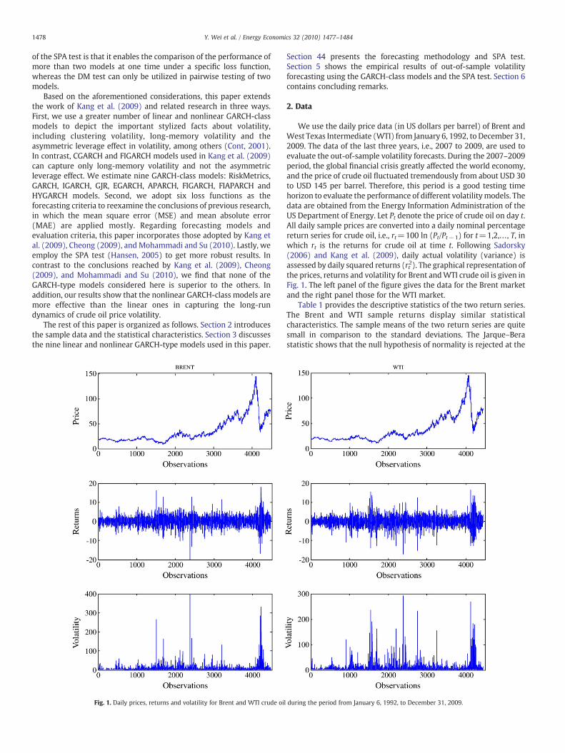
Fig. 1. Daily prices, returns and volatility for Brent and WTI crude oil

Section 44 presents the forecasting methodology and SPA test.Section 5 shows the empirical results of out-of-sample volatilityforecasting using the GARCH-class models and the SPA test. Section 6contains concluding remarks.

2. Data

We use the daily price data (in US dollars per barrel) of Brent andWest Texas Intermediate (WTI) from January 6, 1992, to December 31,2009. The data of the last three years, i.e., 2007 to 2009, are used toevaluate the out-of-sample volatility forecasts. During the 2007–2009period, the global financial crisis greatly affected the world economy,and the price of crude oil fluctuated tremendously from about USD 30to USD 145 per barrel. Therefore, this period is a good testing timehorizon to evaluate the performance of different volatilitymodels. Thedata are obtained from the Energy Information Administration of theUS Department of Energy. Let Pt denote the price of crude oil on day t.All daily sample prices are converted into a daily nominal percentagereturn series for crude oil, i.e., rt=100 ln (Pt/Pt−1) for t=1,2,…, T, inwhich rt is the returns for crude oil at time t. Following Sadorsky(2006) and Kang et al. (2009), daily actual volatility (variance) isassessed by daily squared returns (rt2). The graphical representation ofthe prices, returns and volatility for Brent andWTI crude oil is given inFig. 1. The left panel of the figure gives the data for the Brent marketand the right panel those for the WTI market.

Table 1 provides the descriptive statistics of the two return series.The Brent and WTI sample returns display similar statisticalcharacteristics. The sample means of the two return series are quitesmall in comparison to the standard deviations. The Jarque–Berastatistic shows that the null hypothesis of normality is rejected at the

during the period from January 6, 1992, to December 31, 2009.

Table 1Descriptive statistics for oil price returns.

Brent WTI

Number of observations 4474 4446Mean (%) 0.032 0.032Standard deviation (%) 2.324 2.480Minimum −19.891 −17.092Maximum 18.130 16.414Skewness −0.087 −0.195Excess kurtosis 5.072 4.874Jarque–Bera 4801.221⁎ 4429.502⁎

Q (20) 45.150⁎ 49.208⁎

ADF −16.510⁎ −26.585⁎

P–P −65.450⁎ −67.556⁎

Note: The Jarque–Bera statistic tests for the null hypothesis of normality in the samplereturns distribution. Q (20) is the Ljung–Box statistic of the return series for up to the20th order serial correlation. ADF and P–P are the statistics of the augmented Dickey–Fuller and Phillips–Perron unit root tests, respectively, based on the lowest AIC value.⁎ indicates rejection at the 1% significance level.

1479Y. Wei et al. / Energy Economics 32 (2010) 1477–1484

1% level of significance, also as evidenced by a high excess kurtosisand negative skewness. The Ljung–Box statistic for serial correlationshows that the null hypothesis of no autocorrelation up to the 20thorder is rejected and confirms serial autocorrelation in the crude oilreturns. The augmented Dickey–Fuller and Phillips–Perron unit roottests both support the rejection of the null hypothesis of a unit root atthe 1% significance level, implying that the two return series arestationary and may be modeled directly without further transforms.

3. Model framework

3.1. Linear GARCH-class models

Based on the work of Engle (1982), the most popular volatilitymodel is the GARCH model proposed by Bollerslev (1986). Bollerslevet al. (1994) showed that the GARCH(1,1) specification worked wellin most applied situations, and Sadorsky (2006) also demonstratedthat the GARCH(1,1) model was a good fit for crude oil volatility. Thestandard GARCH(1,1) model for daily returns is given by

rt = μ t + εt = μ t + σtzt ; zteNID 0;1ð Þ;σ2t = ω + αε2t−1 + βσ2

t−1;ð1Þ

where μt denotes the conditional mean and σt2 is the conditional

variance with parameter restrictions ωN0, αN0, βN0 and α+βb1. Asshown in Table 1, the sample mean of crude oil returns is quite smallin comparisonwith its standard deviation (volatility); thus, we set theconditional mean μt to equal 0 in this paper, following Koopman et al.(2005), among others.

Another linear GARCH-class model is the IGARCH model devel-oped by Engle and Bollerslev (1986), which can capture infinitepersistence in the conditional variance. The model setting of theIGARCH(1,1) model is similar to that of the GARCH(1,1) but with theparameter restriction α+β=1. The RiskMetrics volatility specifica-tion of JP Morgan is also popular among market practitioners. In itsmost simple form, the RiskMetrics model is equivalent to a normalIGARCH (1,1) model, where the autoregressive parameter is set at apre-specified value of 0.94 and the coefficient of εt−1

2 is equal to 0.06.In this specification, the conditional variance is defined as

σ2t = 0:06ε2t−1 + 0:94σ2

t−1: ð2Þ

Therefore, the RiskMetrics specification does not require theestimation of unknown parameters in the volatility equation as allparameters are present at given values. Although this is a crudeway tomodel volatility, it is widely used by practitioners as it often givesacceptable short-term volatility forecasts.

In summary, for the linear model setting of the conditionalvariance, we use these three linear GARCH-class models, i.e., theGARCH, IGARCH and RiskMetrics models.

3.2. Nonlinear GARCH-class models

To take the stylized facts of financial markets into account (Cont,2001), other GARCH-class models have been developed to capturelong-memory and short-memory volatility effects, asymmetric lever-age effects and so forth. Because of the nonlinear model setting ofthese newly developed models, we call them nonlinear GARCH-classmodels. The following nonlinear GARCH-class models are used in thispaper to forecast the volatility of crude oil prices.

The GJRmodel developed by Glosten et al. (1993) is constructed tocapture the potential larger impact of negative shocks on returnvolatility, which is usually named as asymmetric leverage volatilityeffect. Specification for the conditional variance of GJR(1,1) model is

σ2t = ω + α + γI εt−1b0ð Þ½ �ε2t−1 + βσ2

t−1; ð3Þ

where I(.) is an indicator function; i.e., when the condition in (.) ismet, I(.)=1, and 0 otherwise. γ is the asymmetric leveragecoefficient, which describes the volatility leverage effect.

Another popular nonlinear GARCH-class model, which can alsodepict the volatility leverage effect, is the exponential GARCH(EGARCH) one proposed by Nelson (1991). Nelson argued that thenonnegative constraints in the linear GARCHmodel are too restrictive.The GARCH model imposes nonnegative constraints on parameters αand β, whereas no restrictions are placed on these parameters in theEGARCH model. The EGARCH(1,1) model is given as

log σ2t

� �= ω + αzt−1 + γ jzt−1j−Ejzt−1j

� �+ β log σ2

t−1

� �; ð4Þ

where γ is again the asymmetric leverage coefficient to describe thevolatility leverage effect.

The asymmetric power ARCH (APARCH) model of Ding et al.(1993) is one of the most promising ARCH-type models. This modelnests several ARCH-type models and has been found to be particularlyrelevant in many recent applications (see, for example, Giot andLaurent, 2003; Mittnik and Paolella, 2000). The APARCH(1,1) model isdefined as follows:

σδt = ω + α jεt−1 j−γεt−1ð Þδ + βσδ

t−1; ð5Þ

where parameter δ (δN0) plays the role of a Box–Cox transformationof the conditional standard deviation σt, while γ reflects the so-calledleverage effect. The APARCH model includes several ARCH extensionsas special cases, including the GARCH(1,1) model when δ=2 andγ=0, and the GJR(1,1) one when δ=2.

As standard GARCH model focuses only on short-term volatilityspecification and forecasting, some authors argue that long-rundependencies (memories) in financial market volatility may be bettercharacterized by a fractionally integrated ARCH (FIGARCH) model(e.g., Andersen and Bollerslev, 1997; Baillie et al., 1996). The FIGARCHmodel implies the finite persistence of volatility shocks (no suchpersistence exists in the GARCH framework), i.e., long-memorybehavior and a slow rate of decay after a volatility shock. An IGARCHmodel implies the complete persistence of a shock, and apparentlyquickly fell out of favor. Interestingly, the FIGARCH(1,d,1) nests aGARCH(1,1) with d=0 and the IGARCH(1,1) for d=1. The FIGARCH(1,d,1) model can be written as follows:

σ2t = ω + βσ2

t−1 + 1− 1−βLð Þ−1 1−φLð Þ 1−Lð Þdh i

ε2t ; ð6Þ

where 0≤d≤1,ωN0,φ, βb1; d is the fractional integration parameterand L is the lag operator. The parameter d characterizes the long-


memory property of hyperbolic decay in volatility because it allowsautocorrelations to decay at a slow hyperbolic rate. The advantage ofthe FIGARCH process is that for 0bdb1, it is sufficiently flexible toallow for intermediate ranges of persistence, between the completeintegrated persistence of volatility shocks associated with d=1 andthe geometric decay associated with d=0.

Subsequently, Tse (1998) developed the fractionally integratedasymmetric power ARCH (FIAPARCH) model, which simultaneouslyallows for long memory and asymmetry in volatility. In the FIAPARCHmodel, the FIGARCH process is modified to allow for asymmetry. TheFIAPARCH(1,d,1) model can then be written as follows:

σδt = ω 1−βð Þ−1 + 1− 1−βLð Þ−1 1−φLð Þ 1−Lð Þd

h ijεt j−γεtð Þδ; ð7Þ

where 0≤d≤1, ω, δN0, φ, βb1 and −1bγb1. The FIAPARCH processis therefore reduced to the FIGARCH one when γ=0 and δ=2.

Davidson (2004) proposed the hyperbolic GARCH (HYGARCH)model, which nests both the GARCH and FIGARCH models as specialcases. The HYGARCH model shares with the GARCH one the desiredproperties of the covariance stationarity while obeying hyperbolicallydecaying impulse response coefficients as does the FIGARCH model.Although proposed only recently, the HYGARCH model has beenproven to be successful in modeling the long-run dynamics in theconditional variance of several financial time series (Davidson, 2004;Tang and Shieh, 2006). The HYGARCH(1,d,1) model is defined asfollows:

σ2t = ω + f1− 1−βL½ �−1φLf1 + k½ 1−Lð Þd−1�ggε2t ; ð8Þ

where 0≤d≤1, ωN0, k≥0, φ, βb1 and L is the lag operator. TheFIGARCH and stable GARCH cases correspond to k=1 and 0,respectively.

Finally, in this paper, we do not consider CGARCH as do Kang et al.(2009) and Agnolucci (2009), as several authors had found that,similar to the CGARCH model, the FIGARCH one can captureconditional variances that reveal not only the short-run dynamics ofthe ARMA type, as in the standard GARCH model, but also the long-run persistence that decays slowly at hyperbolic rates. For example,Maheu (2005) examined whether the CGARCH model was able tocapture the long-range dependence observed in time series volatility.Using several equity and exchange rate returns, he found that the rateof decay implied by the CGARCH model was generally moreappropriate than the exponential decay implied by the GARCH(1,1),but less comparable to that of the FIGARCH(1,d,1) model (Maheu,2005).

In summary, nine linear and nonlinear GARCH-class models, i.e.,RiskMetrics, GARCH, IGARCH, GJR, EGARCH, APARCH, FIGARCH,FIAPARCH and HYGARCH models, are used to describe and forecastthe volatility of Brent and WTI crude oil prices.

4. Forecasting methodology and SPA test

In this section, we evaluate the forecasting performance of the nineGARCH-class models presented in Section 3. The forecasting process ishandled as follows.

The crude oil observations from January 6, 1992, to December 31,2009, of Brent and WTI are classified into two subgroups: the in-sample data for volatility modeling covering a 15-year period, fromJanuary 6, 1992, to December 29, 2006, and the out-of-sample data formodel evaluation covering the period from January 2, 2007, toDecember 31, 2009, i.e., the last three years of the total data sample.The estimation period is then rolled forward by adding one, five ortwenty new day(s) and dropping the most distant day(s). In this way,the sample size used in estimating the models remains fixed and the

forecasts do not overlap. One-, five- and twenty-day out-of-samplevolatility forecasts, corresponding to one-day, one-week and one-month trading periods, are obtained.

As discussed in Section 2, following Sadorsky (2006) and Kang etal. (2009), daily actual volatility (variance) is assessed using the dailysquared returns (rt2) and denoted as σt

2 hereafter. The volatilityforecast obtained using a GARCH-class model is indicated by σ̂

2t .

Various forecasting criteria or loss functions can be considered toassess the predictive accuracy of a volatility model. However, asdiscussed by Lopez (2001), it is not obvious which loss function ismore appropriate for the evaluation of volatilitymodels. Hence, ratherthan making a single choice we use six different accurate statistics orloss functions as forecasting criteria:

MSE = n−1 ∑n

t=1σ2t−σ̂

2t

� �2; ð9Þ

MAE = n−1 ∑n

t=1jσ2

t −σ̂2t j; ð10Þ

HMSE = n−1 ∑n

t=11−σ2

t =σ̂2t

� �2; ð11Þ

HMAE = n−1 ∑n

t=1j1−σ2

t =σ̂2t j; ð12Þ

QLIKE = n−1 ∑n

t=1ln σ̂2

t

� �+ σ2

t =σ̂2t

� �; and ð13Þ

R2LOG = n−1 ∑n

t=1ln σ2

t =σ̂2t

� �h i2; ð14Þ

where n is the number of forecasting data; MSE andMAE are themeansquare error and mean absolute error, respectively; HMSE and HMAEare the MSE and MAE, respectively, adjusted for heteroskedasticity;QLIKE corresponds to the loss implied by a Gaussian likelihood; andR2LOG is similar to the R2 of the Mincer–Zarnowitz regressions.Different criteria serve different practical uses. For example, in thecase of value-at-risk applications, one may be more interested in theaccurate forecasting of a high level of volatility rather than a low level.This implies that the MSE criterion is the relevant loss function for riskmanagement applications. Additional discussion of these criteria canbe found in Bollerslev et al. (1994).

When a particular loss function is smaller for model A than formodel B, we cannot clearly conclude that the forecasting performanceof model A is superior to that of model B. Such a conclusion cannot bemade on the basis of just one loss function and just one sample. Recentwork has focused on a testing framework for determining whether aparticular model is outperformed by another one (e.g., Diebold andMariano, 1995; West, 1996; White, 2000). An extension of the Whiteframework is known as the superior predictive ability (SPA) test,which was proposed by Hansen (2005). The SPA test has been shownto have good power properties and to be more robust than previousapproaches.

In contrast to other evaluation techniques, the SPA test can be usedto compare the performance of two or more forecasting models at atime. Forecasts are evaluated using a pre-specified loss function andthe “best” forecasting model is the one that produces the smallestexpected loss. In a SPA test, the loss function relative to thebenchmark model is defined as Xt, l

(0, i)=Lt, l(0)−Lt,l

(i), where Lt, l(0) is the

value of the loss function l at time t for a benchmark model M0 and Lt,l(i)

is the value of the loss function l at time t for another competitivemodel Mi, for i=1,…,K. The SPA test is used to compare theforecasting performance of a benchmark model against its Kcompetitors. The null hypothesis that the benchmark or base modelis not outperformed by any of the other competitive models can be

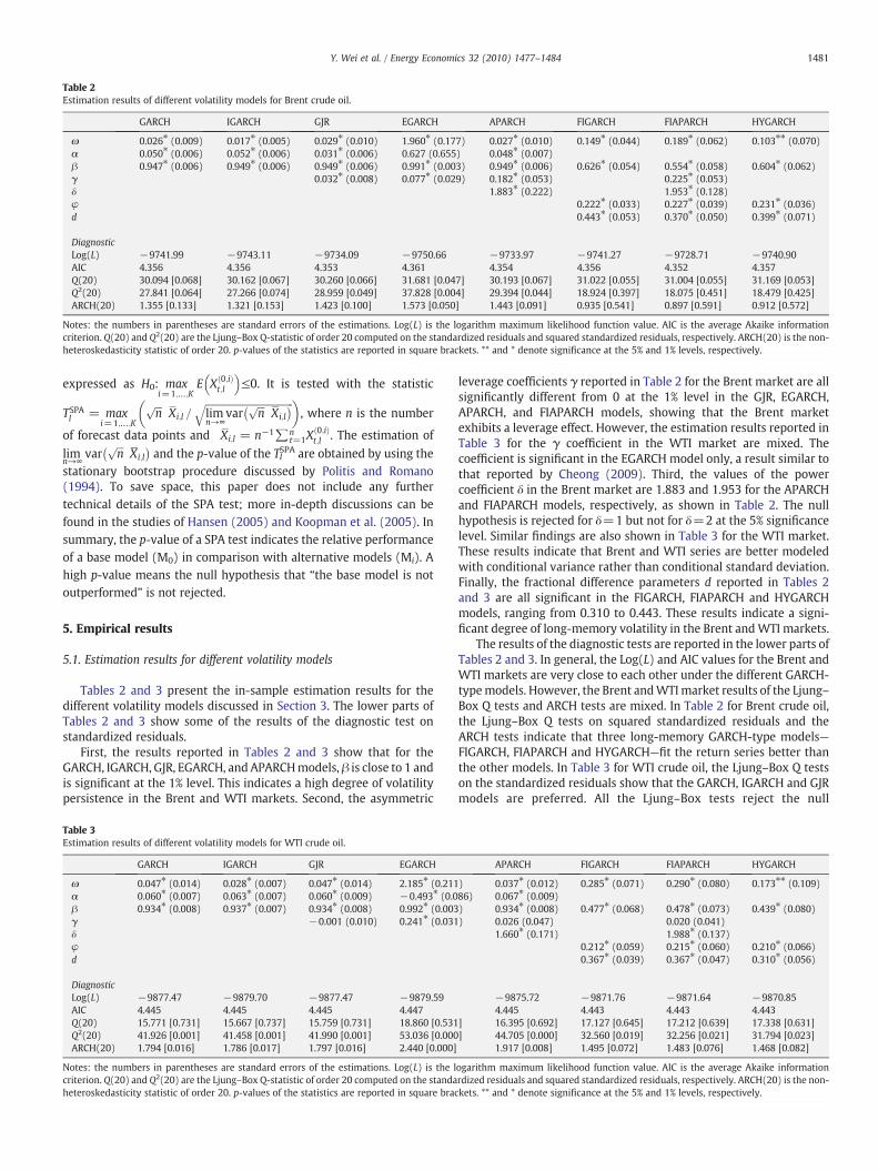
Table 2Estimation results of different volatility models for Brent crude oil.

GARCH IGARCH GJR EGARCH APARCH FIGARCH FIAPARCH HYGARCH

ω 0.026⁎ (0.009) 0.017⁎ (0.005) 0.029⁎ (0.010) 1.960⁎ (0.177) 0.027⁎ (0.010) 0.149⁎ (0.044) 0.189⁎ (0.062) 0.103⁎⁎ (0.070)α 0.050⁎ (0.006) 0.052⁎ (0.006) 0.031⁎ (0.006) 0.627 (0.655) 0.048⁎ (0.007)β 0.947⁎ (0.006) 0.949⁎ (0.006) 0.949⁎ (0.006) 0.991⁎ (0.003) 0.949⁎ (0.006) 0.626⁎ (0.054) 0.554⁎ (0.058) 0.604⁎ (0.062)γ 0.032⁎ (0.008) 0.077⁎ (0.029) 0.182⁎ (0.053) 0.225⁎ (0.053)δ 1.883⁎ (0.222) 1.953⁎ (0.128)φ 0.222⁎ (0.033) 0.227⁎ (0.039) 0.231⁎ (0.036)d 0.443⁎ (0.053) 0.370⁎ (0.050) 0.399⁎ (0.071)

DiagnosticLog(L) −9741.99 −9743.11 −9734.09 −9750.66 −9733.97 −9741.27 −9728.71 −9740.90AIC 4.356 4.356 4.353 4.361 4.354 4.356 4.352 4.357Q(20) 30.094 [0.068] 30.162 [0.067] 30.260 [0.066] 31.681 [0.047] 30.193 [0.067] 31.022 [0.055] 31.004 [0.055] 31.169 [0.053]Q2(20) 27.841 [0.064] 27.266 [0.074] 28.959 [0.049] 37.828 [0.004] 29.394 [0.044] 18.924 [0.397] 18.075 [0.451] 18.479 [0.425]ARCH(20) 1.355 [0.133] 1.321 [0.153] 1.423 [0.100] 1.573 [0.050] 1.443 [0.091] 0.935 [0.541] 0.897 [0.591] 0.912 [0.572]

Notes: the numbers in parentheses are standard errors of the estimations. Log(L) is the logarithm maximum likelihood function value. AIC is the average Akaike informationcriterion. Q(20) and Q2(20) are the Ljung–Box Q-statistic of order 20 computed on the standardized residuals and squared standardized residuals, respectively. ARCH(20) is the non-heteroskedasticity statistic of order 20. p-values of the statistics are reported in square brackets. ** and * denote significance at the 5% and 1% levels, respectively.


expressed as H0: maxi=1;…;K

E X 0;ið Þt;l

� �≤0. It is tested with the statistic

TSPAl = max

i=1;…;K

ffiffiffin

p ―Xi;l =

ffiffiffiffiffiffiffiffiffiffiffiffiffiffiffiffiffiffiffiffiffiffiffiffiffiffiffiffiffiffiffiffiffiffiffiffilimn→∞

varffiffiffin

p ―Xi;l

� �q� �, where n is the number

of forecast data points and―Xi;l = n−1∑n

t=1X0;ið Þt;l . The estimation of

limn→∞

varffiffiffin

p ―Xi;l

� �and the p-value of the Tl

SPA are obtained by using thestationary bootstrap procedure discussed by Politis and Romano(1994). To save space, this paper does not include any furthertechnical details of the SPA test; more in-depth discussions can befound in the studies of Hansen (2005) and Koopman et al. (2005). Insummary, the p-value of a SPA test indicates the relative performanceof a base model (M0) in comparison with alternative models (Mi). Ahigh p-value means the null hypothesis that “the base model is notoutperformed” is not rejected.

5. Empirical results

5.1. Estimation results for different volatility models

Tables 2 and 3 present the in-sample estimation results for thedifferent volatility models discussed in Section 3. The lower parts ofTables 2 and 3 show some of the results of the diagnostic test onstandardized residuals.

First, the results reported in Tables 2 and 3 show that for theGARCH, IGARCH, GJR, EGARCH, and APARCHmodels, β is close to 1 andis significant at the 1% level. This indicates a high degree of volatilitypersistence in the Brent and WTI markets. Second, the asymmetric

Table 3Estimation results of different volatility models for WTI crude oil.

GARCH IGARCH GJR EGARCH

ω 0.047⁎ (0.014) 0.028⁎ (0.007) 0.047⁎ (0.014) 2.185⁎ (0.211α 0.060⁎ (0.007) 0.063⁎ (0.007) 0.060⁎ (0.009) −0.493⁎ (0.0β 0.934⁎ (0.008) 0.937⁎ (0.007) 0.934⁎ (0.008) 0.992⁎ (0.003γ −0.001 (0.010) 0.241⁎ (0.031δφd

DiagnosticLog(L) −9877.47 −9879.70 −9877.47 −9879.59AIC 4.445 4.445 4.445 4.447Q(20) 15.771 [0.731] 15.667 [0.737] 15.759 [0.731] 18.860 [0.531Q2(20) 41.926 [0.001] 41.458 [0.001] 41.990 [0.001] 53.036 [0.000ARCH(20) 1.794 [0.016] 1.786 [0.017] 1.797 [0.016] 2.440 [0.000]

Notes: the numbers in parentheses are standard errors of the estimations. Log(L) is the lcriterion. Q(20) and Q2(20) are the Ljung–Box Q-statistic of order 20 computed on the standaheteroskedasticity statistic of order 20. p-values of the statistics are reported in square brac

leverage coefficients γ reported in Table 2 for the Brent market are allsignificantly different from 0 at the 1% level in the GJR, EGARCH,APARCH, and FIAPARCH models, showing that the Brent marketexhibits a leverage effect. However, the estimation results reported inTable 3 for the γ coefficient in the WTI market are mixed. Thecoefficient is significant in the EGARCH model only, a result similar tothat reported by Cheong (2009). Third, the values of the powercoefficient δ in the Brent market are 1.883 and 1.953 for the APARCHand FIAPARCH models, respectively, as shown in Table 2. The nullhypothesis is rejected for δ=1 but not for δ=2 at the 5% significancelevel. Similar findings are also shown in Table 3 for the WTI market.These results indicate that Brent and WTI series are better modeledwith conditional variance rather than conditional standard deviation.Finally, the fractional difference parameters d reported in Tables 2and 3 are all significant in the FIGARCH, FIAPARCH and HYGARCHmodels, ranging from 0.310 to 0.443. These results indicate a signi-ficant degree of long-memory volatility in the Brent andWTI markets.

The results of the diagnostic tests are reported in the lower parts ofTables 2 and 3. In general, the Log(L) and AIC values for the Brent andWTI markets are very close to each other under the different GARCH-typemodels. However, the Brent andWTImarket results of the Ljung–Box Q tests and ARCH tests are mixed. In Table 2 for Brent crude oil,the Ljung–Box Q tests on squared standardized residuals and theARCH tests indicate that three long-memory GARCH-type models—FIGARCH, FIAPARCH and HYGARCH—fit the return series better thanthe other models. In Table 3 for WTI crude oil, the Ljung–Box Q testson the standardized residuals show that the GARCH, IGARCH and GJRmodels are preferred. All the Ljung–Box tests reject the null

APARCH FIGARCH FIAPARCH HYGARCH

) 0.037⁎ (0.012) 0.285⁎ (0.071) 0.290⁎ (0.080) 0.173⁎⁎ (0.109)86) 0.067⁎ (0.009)) 0.934⁎ (0.008) 0.477⁎ (0.068) 0.478⁎ (0.073) 0.439⁎ (0.080)) 0.026 (0.047) 0.020 (0.041)

1.660⁎ (0.171) 1.988⁎ (0.137)0.212⁎ (0.059) 0.215⁎ (0.060) 0.210⁎ (0.066)0.367⁎ (0.039) 0.367⁎ (0.047) 0.310⁎ (0.056)

−9875.72 −9871.76 −9871.64 −9870.854.445 4.443 4.443 4.443

] 16.395 [0.692] 17.127 [0.645] 17.212 [0.639] 17.338 [0.631]] 44.705 [0.000] 32.560 [0.019] 32.256 [0.021] 31.794 [0.023]

1.917 [0.008] 1.495 [0.072] 1.483 [0.076] 1.468 [0.082]

ogarithm maximum likelihood function value. AIC is the average Akaike informationrdized residuals and squared standardized residuals, respectively. ARCH(20) is the non-kets. ** and * denote significance at the 5% and 1% levels, respectively.

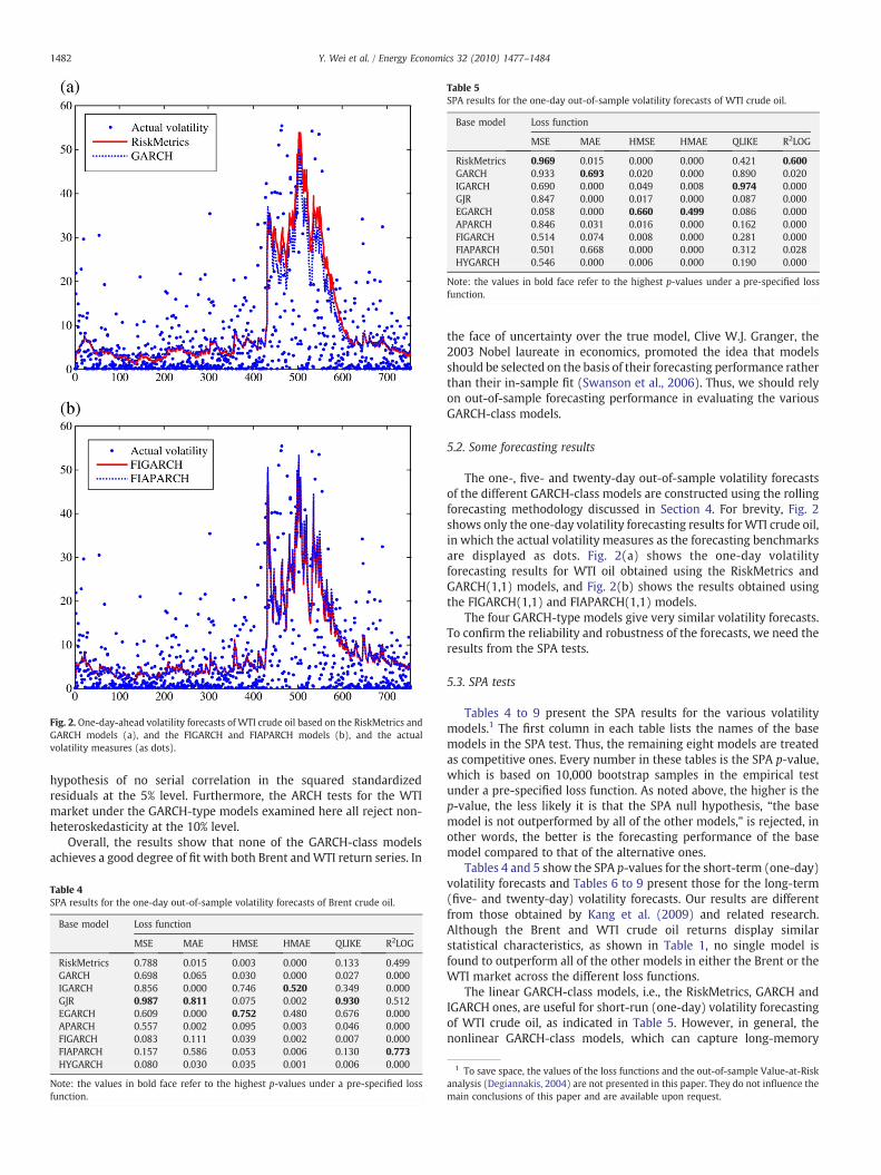
Fig. 2. One-day-ahead volatility forecasts of WTI crude oil based on the RiskMetrics andGARCH models (a), and the FIGARCH and FIAPARCH models (b), and the actualvolatility measures (as dots).

Table 5SPA results for the one-day out-of-sample volatility forecasts of WTI crude oil.

Base model Loss function

MSE MAE HMSE HMAE QLIKE R2LOG

RiskMetrics 0.969 0.015 0.000 0.000 0.421 0.600GARCH 0.933 0.693 0.020 0.000 0.890 0.020IGARCH 0.690 0.000 0.049 0.008 0.974 0.000GJR 0.847 0.000 0.017 0.000 0.087 0.000EGARCH 0.058 0.000 0.660 0.499 0.086 0.000APARCH 0.846 0.031 0.016 0.000 0.162 0.000FIGARCH 0.514 0.074 0.008 0.000 0.281 0.000FIAPARCH 0.501 0.668 0.000 0.000 0.312 0.028HYGARCH 0.546 0.000 0.006 0.000 0.190 0.000

Note: the values in bold face refer to the highest p-values under a pre-specified lossfunction.


hypothesis of no serial correlation in the squared standardizedresiduals at the 5% level. Furthermore, the ARCH tests for the WTImarket under the GARCH-type models examined here all reject non-heteroskedasticity at the 10% level.

Overall, the results show that none of the GARCH-class modelsachieves a good degree of fit with both Brent andWTI return series. In

Table 4SPA results for the one-day out-of-sample volatility forecasts of Brent crude oil.





the face of uncertainty over the true model, Clive W.J. Granger, the2003 Nobel laureate in economics, promoted the idea that modelsshould be selected on the basis of their forecasting performance ratherthan their in-sample fit (Swanson et al., 2006). Thus, we should relyon out-of-sample forecasting performance in evaluating the variousGARCH-class models.

5.2. Some forecasting results

The one-, five- and twenty-day out-of-sample volatility forecastsof the different GARCH-class models are constructed using the rollingforecasting methodology discussed in Section 4. For brevity, Fig. 2shows only the one-day volatility forecasting results forWTI crude oil,in which the actual volatility measures as the forecasting benchmarksare displayed as dots. Fig. 2(a) shows the one-day volatilityforecasting results for WTI oil obtained using the RiskMetrics andGARCH(1,1) models, and Fig. 2(b) shows the results obtained usingthe FIGARCH(1,1) and FIAPARCH(1,1) models.

The four GARCH-type models give very similar volatility forecasts.To confirm the reliability and robustness of the forecasts, we need theresults from the SPA tests.

5.3. SPA tests

Tables 4 to 9 present the SPA results for the various volatilitymodels.1 The first column in each table lists the names of the basemodels in the SPA test. Thus, the remaining eight models are treatedas competitive ones. Every number in these tables is the SPA p-value,which is based on 10,000 bootstrap samples in the empirical testunder a pre-specified loss function. As noted above, the higher is thep-value, the less likely it is that the SPA null hypothesis, “the basemodel is not outperformed by all of the other models,” is rejected, inother words, the better is the forecasting performance of the basemodel compared to that of the alternative ones.

Tables 4 and 5 show the SPA p-values for the short-term (one-day)volatility forecasts and Tables 6 to 9 present those for the long-term(five- and twenty-day) volatility forecasts. Our results are differentfrom those obtained by Kang et al. (2009) and related research.Although the Brent and WTI crude oil returns display similarstatistical characteristics, as shown in Table 1, no single model isfound to outperform all of the other models in either the Brent or theWTI market across the different loss functions.

The linear GARCH-class models, i.e., the RiskMetrics, GARCH andIGARCH ones, are useful for short-run (one-day) volatility forecastingof WTI crude oil, as indicated in Table 5. However, in general, thenonlinear GARCH-class models, which can capture long-memory

1 To save space, the values of the loss functions and the out-of-sample Value-at-Riskanalysis (Degiannakis, 2004) are not presented in this paper. They do not influence themain conclusions of this paper and are available upon request.

image of Fig.�2

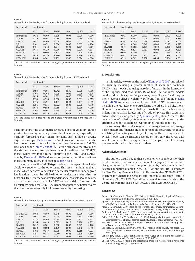
Table 6SPA results for the five-day out-of-sample volatility forecasts of Brent crude oil.





Table 7SPA results for the five-day out-of-sample volatility forecasts of WTI crude oil.





Table 9SPA results for the twenty-day out-of-sample volatility forecasts of WTI crude oil.






volatility and/or the asymmetric leverage effect in volatility, exhibitgreater forecasting accuracy than the linear ones, especially involatility forecasting over longer horizons, such as five or twentydays. For example, Tables 6 and 8 (Brent crude oil) indicate that thebest models across the six loss functions are the nonlinear GARCH-class ones, while Tables 7 and 9 (WTI crude oil) show that five out ofthe six best models are nonlinear ones. In addition, the FIGARCHmodel, which was found to be superior to the GARCH and IGARCHones by Kang et al. (2009), does not outperform the other nonlinearmodels in many cases, as shown in Tables 4 to 9.

In short, none of the GARCH-typemodels in this paper is found to beabsolutely superior to the other ones. This result reminds us that amodel which performs very well in a particularmarket or under a givenloss function may not be reliable in other markets or under other lossfunctions. Thus, energy economists andfinancial analysts shouldbeverycautious when using a particular GARCH-class model to forecast crudeoil volatility. Nonlinear GARCH-classmodels appear to be better choicesthan linear ones, especially for long-run volatility forecasting.

Table 8SPA results for the twenty-day out-of-sample volatility forecasts of Brent crude oil.





6. Conclusions

In this article, we extend the work of Kang et al. (2009) and relatedresearch by including a greater number of linear and nonlinearGARCH-class models and using more loss functions in the frameworkof the superior predictive ability (SPA) test. The nonlinear modelsconsidered herein capture long-memory volatility and/or the asym-metry leverage effect in volatility. Different from the finding of Kanget al. (2009) and related research, none of the GARCH-class models,including the FIGARCH one, outperforms the others in all situations.However, the nonlinearmodels do perform better than the linear onesin long-run volatility forecasting of crude oil prices. This paper alsoanswers the question posed by Agnolucci (2009) about “whether thecomparison of volatility forecasting models is influenced by thecriterion used in the exercise.” Our findings indicate that it is.

In summary, the results suggest that energy economists, energypolicymakers and financial practitioners should not arbitrarily choosea volatility forecasting model by referring to the existing research.Which model can be trusted depends on not only the given datasample but also the correspondence of the particular forecastingpurpose with the loss function considered.

Acknowledgements

The authors would like to thank the anonymous referees for theirhelpful comments on an earlier version of the paper. The authors arealso grateful for the financial support offered by the National NaturalScience Foundation of China (Nos. 70501025 and 70771097), Programfor New Century Excellent Talents in University (No. NCET-08-0826),Program for Changjiang Scholars and Innovative Research Team inUniversity (No. PCSIRT0860) and Fundamental Research Funds for theCentral Universities (Nos. SWJTU09ZT32 and SWJTU09CX088).

References

Adrangi, B., Chatrath, A., Dhanda, K.K., Raffiee, K., 2001. Chaos in oil prices? Evidencefrom futures markets. Energy Economics 23, 405–425.

Agnolucci, P., 2009. Volatility in crude oil futures: a comparison of the predictive abilityof GARCH and implied volatility models. Energy Economics 31, 316–321.

Aloui, C., Mabrouk, S., 2010. Value-at-risk estimations of energy commodities via long-memory, asymmetry and fat-tailed GARCH models. Energy Policy 38, 2326–2339.

Andersen, T.G., Bollerslev, T., 1997. Intraday periodicity and volatility persistence infinancial markets. Journal of Empirical Finance 4, 115–158.

Baillie, R.T., Bollerslev, T., Mikkelsen, H.O., 1996. Fractionally integrated generalizedautoregressive conditional heteroskedasticity. Journal of Econometrics 74, 3–30.

Bollerslev, T., 1986. Generalized autoregressive conditional heteroskedasticity. Journalof Econometrics 31, 307–327.

Bollerslev, T., Engle, R.F., Nelson, D., 1994. ARCH models. In: Engle, R.F., McFadden, D.L.(Eds.), Handbook of Econometrics, vol. IV. Elsevier Science BV, Amsterdam, pp.2961–3038.

Cabedo, J.D., Moya, I., 2003. Estimating oil price ‘Value at Risk’ using the historicalsimulation approach. Energy Economics 25, 239–253.

Cheong, C.W., 2009. Modeling and forecasting crude oil markets using ARCH-typemodels. Energy Policy 37, 2346–2355.


Cont, R., 2001. Empirical properties of asset returns: stylized facts and statistical issues.Quantitative Finance 1, 223–236.

Davidson, J., 2004. Moment and memory properties of linear conditional hetero-scedasticity models, and a newmodel. Journal of Business & Economic Statistics 22,16–29.

Degiannakis, S., 2004. Volatility forecasting: Evidence from a fractional integratedasymmetric power ARCH skewed-t model. Applied Financial Economics 14,1333–1342.

Diebold, F.X., Mariano, R.S., 1995. Comparing predictive accuracy. Journal of Business &Economic Statistics 13, 253–263.

Ding, Z., Granger, C.W.J., Engle, R.F., 1993. A long memory property of stock marketreturns and a new model. Journal of Empirical Finance 1, 83–106.

Engle, R.F., 1982. Autoregressive conditional heteroskedasticity with estimates of thevariance of United Kingdom inflation. Econometrica 50, 987–1007.

Engle, R.F., Bollerslev, T., 1986. Modelling the persistence of conditional variances.Econometric Reviews 5, 1–50.

Fong, W.M., See, K.H., 2002. A Markov switching model of the conditional volatility ofcrude oil futures prices. Energy Economics 24, 71–95.

Giot, P., Laurent, S., 2003. Market risk in commodity markets: a VaR approach. EnergyEconomics 25, 435–457.

Glosten, L.R., Jagannathan, R., Runkle, D.E., 1993. On the relation between the expectedvalue and the volatility of the nominal excess return on stocks. Journal of Finance48, 1779–1801.

Hansen, P.R., 2005. A test for superior predictive ability. Journal of Business & EconomicStatistics 23, 365–380.

Kang, S.H., Kang, S.M., Yoon, S.M., 2009. Forecasting volatility of crude oil markets.Energy Economics 31, 119–125.

Kolos, S.P., Ronn, E.I., 2008. Estimating the commodity market price of risk for energyprices. Energy Economics 30, 621–641.

Koopman, S.J., Jungbacker, B., Hol, E., 2005. Forecasting daily variability of the S&P100stock index using historical, realized and implied volatility measurements. Journalof Empirical Finance 12, 445–475.

Lopez, J.A., 2001. Evaluating the predictive accuracy of volatility models. Journal ofForecasting 20, 87–109.

Maheu, J., 2005. Can GARCH models capture long-range dependence? Studies inNonlinear Dynamics & Econometrics 9 (4), 1269.

Mittnik, S., Paolella, M., 2000. Conditional density and Value-at-Risk prediction of Asiancurrency exchange rates. Journal of Forecasting 19, 313–333.

Mohammadi, H., Su, L., 2010. International evidence on crude oil price dynamics:applications of ARIMA–GARCH models. Energy Economics 32 (5), 1001–1008.

Morana, C., 2001. A semiparametric approach to short-term oil price forecasting.Energy Economics 23, 325–338.

Narayan, P.K., Narayan, S., 2007. Modelling oil price volatility. Energy Policy 35, 6549–6553.Nelson, D.B., 1991. Conditional heteroskedasticity in asset returns: a new approach.

Econometrica 59, 347–370.Politis, D.N., Romano, J.P., 1994. The stationary bootstrap. Journal of the American

Statistical Association 89, 1303–1313.Sadeghi, M., Shavvalpour, S., 2006. Energy risk management and value at risk modeling.

Energy Policy 34, 3367–3373.Sadorsky, P., 2006. Modeling and forecasting petroleum futures volatility. Energy

Economics 28, 467–488.Swanson, N.R., Elliott, G., Ghysels, E., Gonzalo, J., 2006. Predictive methodology and

application in economics and finance: volume in honor of the accomplishments ofClive W.J. Granger. Journal of Econometrics 135, 1–9.

Tang, T.-L., Shieh, S.-J., 2006. Long memory in stock index future markets: a value-at-risk approach. Physica A 366, 437–448.

Tse, Y.K., 1998. The conditional heteroscedasticity of the Yen–Dollar exchange rate.Journal of Applied Econometrics 13, 49–55.

West, K.D., 1996. Asymptotic inference about predictive ability. Econometrica 64,1067–1084.

White, H., 2000. A reality check for data snooping. Econometrica 68, 1097–1126.

Download - Forecasting crude oil market volatility: Further evidence using GARCH-class models

Top Related